
Center for Economic Research and Graduate Education
Charles University
Economics Institute
Academy of Science of the Czech Republic
A COOK-BOOK OF
MATHEMATICS
Viatcheslav VINOGRADOV
June 1999
CERGE-EI LECTURE NOTES
1


A Cook-Book of
MAT HEMAT ICS
Viatcheslav Vinogradov
Center for Economic Research and Graduate Education
and Economics Institute of the Czech Academy of Sciences,
Prague, 1999

CERGE-EI 1999
ISBN 80-86286-20-7

To my Teachers

He liked those literary cooks
Who skim the cream of others’ books
And ruin half an author’s graces
By plucking bon-mots from their places.
Hannah More, Florio (1786)
Introduction
This textbook is based on an extended collection of handouts I distributed to the graduate
students in economics attending my summer mathematics class at the Center for Economic
Research and Graduate Education (CERGE) at Charles University in Prague.
Two considerations motivated me to write this book. First, I wanted to write a short
textbook, which could be covered in the course of two months and which, in turn, covers
the most significant issues of mathematical economics. I have attempted to maintain a
balance between being overly detailed and overly schematic. Therefore this text should
resemble (in the ‘ideological’ sense) a “hybrid” of Chiang’s classic textbook Fundamental
Methods of Mathematical Economics and the comprehensive reference manual by Berck
and Sydsæter (Exact references appear at the end of this section).
My second objective in writing this text was to provide my students with simple “cook-
book” recipes for solving problems they might face in their studies of economics. Since the
target audience was supposed to have some mathematical background (admittance to the
program requires at least BA level mathematics), my main goal was to refresh students’
knowledge of mathematics rather than teach them math ‘from scratch’. Students were
expected to be familiar with the basics of set theory, the real-number system, the concept
of a function, polynomial, rational, exponential and logarithmic functions, inequalities
and absolute values.
Bearing in mind the applied nature of the course, I usually refrained from presenting
complete proofs of theoretical statements. Instead, I chose to allocate more time and
space to examples of problems and their solutions and economic applications. I strongly
believe that for students in economics – for whom this text is meant – the application
of mathematics in their studies takes precedence over das Glasperlenspiel of abstract
theoretical constructions.
Mathematics is an ancient science and, therefore, it is little wonder that these notes
may remind the reader of the other text-books which have already been written and
published. To be candid, I did not intend to be entirely original, since that would be
impossible.
On the contrary, I tried to benefit from books already in existence and
adapted some interesting examples and worthy pieces of theory presented there. If the
reader requires further proofs or more detailed discussion, I have included a useful, but
hardly exhaustive reference guide at the end of each section.
With very few exceptions, the analysis is limited to the case of real numbers, the
theory of complex numbers being beyond the scope of these notes.
Finally, I would like to express my deep gratitude to Professor Jan Kmenta for his
valuable comments and suggestions, to Sufana Razvan for his helpful assistance, to Aurelia
Pontes for excellent editorial support, to Natalka Churikova for her advice and, last but
not least, to my students who inspired me to write this book.
All remaining mistakes and misprints are solely mine.
i

I wish you success in your mathematical kitchen! Bon Appetit !
Supplementary Reading (General):
• Arrow, K. and M.Intriligator, eds. Handbook of Mathematical Economics, vol. 1.
• Berck P. and K. Sydsæter. Economist’s Mathematical Manual.
• Chiang, A. Fundamental Methods of Mathematical Economics.
• Ostaszewski, I. Mathematics in Economics: Models and Methods.
• Samuelson, P. Foundations of Economic Analysis.
• Silberberg, E. The Structure of Economics: A Mathematical Analysis.
• Takayama, A. Mathematical Economics.
• Yamane, T. Mathematics for Economists: An Elementary Survey.
ii

Basic notation used in the text:
Statements:
A, B, C, . . .
True/False: all statements are either true or false.
Negation:
¬A
‘not A’
Conjunction:
A
∧ B
‘A and B’
Disjunction:
A
∨ B
‘A or B’
Implication:
A
⇒ B
‘A implies B’
(A is sufficient condition for B; B is necessary condition for A.)
Equivalence:
A
⇔ B
‘A if and only if B’ (A iff B, for short)
(A is necessary and sufficient for B; B is necessary and sufficient for A.)
Example 1
(
¬A) ∧ A ⇔ FALSE.
(
¬(A ∨ B)) ⇔ ((¬A) ∧ (¬B)) (De Morgan rule).
Quantifiers:
Existential:
∃
‘There exists’ or ‘There is’
Universal:
∀
‘For all’ or ‘For every’
Uniqueness:
∃!
‘There exists a unique ...’ or ‘There is a unique...’
The colon :
and the vertical line
| are widely used as abbreviations for ‘such that’
a
∈ S means ‘a is an element of (belongs to) set S’
Example 2 (Definition of continuity)
f is continuous at x if
((
∀ > 0)(∃δ > 0) : (∀y ∈ |y − x| < δ ⇒ |f(y) − f(x)| < )
Optional information which might be helpful is typeset in
footnotesize
font.
The symbol
4
!
is used to draw the reader’s attention to potential pitfalls.
iii

Contents
1
Linear Algebra
1
1.1
Matrix Algebra . . . . . . . . . . . . . . . . . . . . . . . . . . . . . . . . .
1
1.1.1
Matrix Operations . . . . . . . . . . . . . . . . . . . . . . . . . . .
1
1.1.2
Laws of Matrix Operations . . . . . . . . . . . . . . . . . . . . . . .
2
1.1.3
Inverses and Transposes . . . . . . . . . . . . . . . . . . . . . . . .
3
1.1.4
Determinants and a Test for Non-Singularity . . . . . . . . . . . . .
4
1.1.5
Rank of a Matrix . . . . . . . . . . . . . . . . . . . . . . . . . . . .
7
1.2
Systems of Linear Equations . . . . . . . . . . . . . . . . . . . . . . . . . .
8
1.3
Quadratic Forms . . . . . . . . . . . . . . . . . . . . . . . . . . . . . . . .
11
1.4
Eigenvalues and Eigenvectors
. . . . . . . . . . . . . . . . . . . . . . . . .
13
1.5
Appendix: Vector Spaces . . . . . . . . . . . . . . . . . . . . . . . . . . . .
15
1.5.1
Basic Concepts . . . . . . . . . . . . . . . . . . . . . . . . . . . . .
15
1.5.2
Vector Subspaces . . . . . . . . . . . . . . . . . . . . . . . . . . . .
17
1.5.3
Independence and Bases . . . . . . . . . . . . . . . . . . . . . . . .
17
1.5.4
Linear Transformations and Changes of Bases . . . . . . . . . . . .
18
2
Calculus
21
2.1
The Concept of Limit . . . . . . . . . . . . . . . . . . . . . . . . . . . . . .
21
2.2
Differentiation - the Case of One Variable
. . . . . . . . . . . . . . . . . .
22
2.3
Rules of Differentiation . . . . . . . . . . . . . . . . . . . . . . . . . . . . .
24
2.4
Maxima and Minima of a Function of One Variable . . . . . . . . . . . . .
26
2.5
Integration (The Case of One Variable) . . . . . . . . . . . . . . . . . . . .
29
2.6
Functions of More than One Variable . . . . . . . . . . . . . . . . . . . . .
32
2.7
Unconstrained Optimization in the Case of More than One Variable . . . .
34
2.8
The Implicit Function Theorem . . . . . . . . . . . . . . . . . . . . . . . .
35
2.9
Concavity, Convexity, Quasiconcavity and Quasiconvexity . . . . . . . . . .
38
2.10 Appendix: Matrix Derivatives . . . . . . . . . . . . . . . . . . . . . . . . .
40
3
Constrained Optimization
43
3.1
Optimization with Equality Constraints . . . . . . . . . . . . . . . . . . . .
43
3.2
The Case of Inequality Constraints . . . . . . . . . . . . . . . . . . . . . .
47
3.2.1
Non-Linear Programming
. . . . . . . . . . . . . . . . . . . . . . .
47
3.2.2
Kuhn-Tucker Conditions . . . . . . . . . . . . . . . . . . . . . . . .
49
3.3
Appendix: Linear Programming . . . . . . . . . . . . . . . . . . . . . . . .
54
3.3.1
The Setup of the Problem . . . . . . . . . . . . . . . . . . . . . . .
54
3.3.2
The Simplex Method . . . . . . . . . . . . . . . . . . . . . . . . . .
55
3.3.3
Duality
. . . . . . . . . . . . . . . . . . . . . . . . . . . . . . . . .
61
4
Dynamics
63
4.1
Differential Equations . . . . . . . . . . . . . . . . . . . . . . . . . . . . . .
63
4.1.1
Differential Equations of the First Order . . . . . . . . . . . . . . .
63
4.1.2
Linear Differential Equations of a Higher Order with Constant Co-
efficients . . . . . . . . . . . . . . . . . . . . . . . . . . . . . . . . .
65
4.1.3
Systems of the First Order Linear Differential Equations . . . . . .
68
4.1.4
Simultaneous Differential Equations. Types of Equilibria . . . . . .
77
4.2
Difference Equations . . . . . . . . . . . . . . . . . . . . . . . . . . . . . .
79
iv

4.2.1
First-order Linear Difference Equations . . . . . . . . . . . . . . . .
80
4.2.2
Second-Order Linear Difference Equations . . . . . . . . . . . . . .
82
4.2.3
The General Case of Order n
. . . . . . . . . . . . . . . . . . . . .
83
4.3
Introduction to Dynamic Optimization . . . . . . . . . . . . . . . . . . . .
85
4.3.1
The First-Order Conditions . . . . . . . . . . . . . . . . . . . . . .
85
4.3.2
Present-Value and Current-Value Hamiltonians
. . . . . . . . . . .
87
4.3.3
Dynamic Problems with Inequality Constraints
. . . . . . . . . . .
87
5
Exercises
93
5.1
Solved Problems
. . . . . . . . . . . . . . . . . . . . . . . . . . . . . . . .
93
5.2
More Problems . . . . . . . . . . . . . . . . . . . . . . . . . . . . . . . . .
99
5.3
Sample Tests
. . . . . . . . . . . . . . . . . . . . . . . . . . . . . . . . . . 101
v

1
Linear Algebra
1.1
Matrix Algebra
Definition 1 An m
× n matrix is a rectangular array of real numbers with m rows and
n columns.
A =
a
11
a
12
. . . a
1n
a
21
a
22
. . . a
2n
..
.
..
.
..
.
a
m1
a
m2
. . . a
mn
,
m
× n is called the dimension or order of A. If m = n, the matrix is the square of order
n.
A subscribed element of a matrix is always read as a
row,column
4
!
A shorthand notation is A = (a
ij
), i = 1, 2, . . . , m and j = 1, 2, . . . , n, or A =
(a
ij
)
[m
×n]
.
A vector is a special case of a matrix, when either m = 1 (row vectors v = (v
1
, v
2
, . . . , v
n
))
or n = 1 – column vectors
u =
u
1
u
2
..
.
u
m
.
1.1.1
Matrix Operations
• Addition and subtraction: given A = (a
ij
)
[m
×n]
and B = (b
ij
)
[m
×n]
A
± B = (a
ij
± b
ij
)
[m
×n]
,
i.e. we simply add or subtract corresponding elements.
Note that these operations are defined only if A and B are of the same dimension.
4
!
• Scalar multiplication:
λA = (λa
ij
),
where λ
∈ R,
i.e. each element of A is multiplied by the same scalar λ.
• Matrix multiplication: if A = (a
ij
)
[m
×n]
and B = (a
ij
)
[n
×k]
then
A
· B = C = (c
ij
)
[m
×k]
,
where c
ij
=
n
X
l=1
a
il
b
lj
.
Note the dimensions of matrices!
4
!
Recipe 1 – How to Multiply Two Matrices:
In order to get the element c
ij
of matrix C you need to multiply the ith row of matrix
A by the jth column of matrix B.
1

Example 3
3 2 1
4 5 6
!
·
9 10
12 11
14 13
=
3
· 9 + 2 · 12 + 1 · 14 3 · 10 + 2 · 11 + 1 · 13
4
· 9 + 5 · 12 + 6 · 14 4 · 10 + 5 · 11 + 6 · 13
!
.
Example 4 A system of m linear equations for n unknowns
a
11
x
1
+ a
12
x
2
+ . . . + a
1n
x
n
=
b
1
,
. . .
..
.
a
m1
x
1
+ a
m2
x
2
+ . . . + a
mn
x
n
= b
m
,
can be written as Ax = b, where A = (a
ij
)
[m
×n]
, and
x =
x
1
..
.
x
n
,
b =
b
1
..
.
b
m
.
1.1.2
Laws of Matrix Operations
• Commutative law of addition: A + B = B + A.
• Associative law of addition: (A + B) + C = A + (B + C).
• Associative law of multiplication: A(BC) = (AB)C.
• Distributive law:
A(B + C) = AB + AC (premultiplication by A),
(B + C)A = BA + BC (postmultiplication by A).
The commutative law of multiplication is not applicable in the matrix case, AB
6=
BA!!!
4
!
Example 5
Let
A =
2 0
3 8
!
,
B =
7 2
6 3
!
.
Then
AB =
14
4
69 30
!
6= BA =
20 16
21 24
!
.
Example 6
Let
v = (v
1
, v
2
, . . . , v
n
),
u =
u
1
u
2
..
.
u
n
.
Then vu = v
1
u
1
+ v
2
u
2
+ . . . + v
n
u
n
is a scalar, and uv = C = (c
ij
)
[n
×n]
is a n by n
matrix, with c
ij
= u
i
v
j
, i, j = 1, . . . , n.
We introduce the identity or unit matrix of dimension n I
n
as
I
n
=
1 0 . . . 0
0 1 . . . 0
..
.
..
.
. .. ...
0 0 . . . 1
.
Note that I
n
is always a square [n
×n] matrix (further on the subscript n will be omitted).
I
n
has the following properties:
2

a) AI = IA = A,
b) AIB = AB for all A, B.
In this sense the identity matrix corresponds to 1 in the case of scalars.
The null matrix is a matrix of any dimension for which all elements are zero:
0 =
0 . . . 0
..
.
. .. ...
0 . . . 0
.
Properties of a null matrix:
a) A + 0 = A,
b) A + (
−A) = 0.
Note that AB = 0
6⇒ A = 0 or B = 0;
AB = AC
6⇒ B = C.
4
!
Definition 2 A diagonal matrix is a square matrix whose only non-zero elements appear
on the principle (or main) diagonal.
A triangular matrix is a square matrix which has only zero elements above or below
the principle diagonal.
1.1.3
Inverses and Transposes
Definition 3 We say that B = (b
ij
)
[n
×m]
is the transpose of A = (a
ij
)
[m
×n]
if a
ji
= b
ij
for all i = 1, . . . , n and j = 1, . . . , m.
Usually transposes are denoted as A
0
(or as A
T
).
Recipe 2 – How to Find the Transpose of a Matrix:
The transpose A
0
of A is obtained by making the columns of A into the rows of A
0
.
Example 7
A =
1 2 3
0 a b
!
,
A
0
=
1 0
2 a
3 b
.
Properties of transposition:
a) (A
0
)
0
= A
b) (A + B)
0
= A
0
+ B
0
c) (αA)
0
= αA
0
, where α is a real number.
d) (AB)
0
= B
0
A
0
Note the order of transposed matrices!
4
!
Definition 4 If A
0
= A, A is called symmetric.
If A
0
=
−A, A is called anti-symmetric (or skew-symmetric).
If A
0
A = I, A is called orthogonal.
If A = A
0
and AA = A, A is called idempotent.
3

Definition 5 The inverse matrix A
−1
is defined as A
−1
A = AA
−1
= I.
Note that A as well as A
−1
are square matrices of the same dimension (it follows from
the necessity to have the preceding line defined).
4
!
Example 8
If
A =
1 2
3 4
!
then the inverse of A is
A
−1
=
−2
1
3
2
−
1
2
!
.
We can easily check that
1 2
3 4
!
−2
1
3
2
−
1
2
!
=
−2
1
3
2
−
1
2
!
1 2
3 4
!
=
1 0
0 1
!
.
Another important characteristics of inverse matrices and inversion:
• Not all square matrices have their inverses. If a square matrix has its inverse, it is
called regular or non-singular. Otherwise it is called singular matrix.
• If A
−1
exists, it is unique.
• A
−1
A = I is equivalent to AA
−1
= I.
Properties of inversion:
a) (A
−1
)
−1
= A
b) (αA)
−1
=
1
α
A
−1
, where α is a real number, α
6= 0.
c) (AB)
−1
= B
−1
A
−1
Note the order of matrices!
4
!
d) (A
0
)
−1
= (A
−1
)
0
1.1.4
Determinants and a Test for Non-Singularity
The formal definition of the determinant is as follows: given n
× n matrix A = (a
ij
),
det(A) =
X
(α
1
,...,α
n
)
(
−1)
I(α
1
,...,α
n
)
a
1α
1
· a
2α
2
· . . . · a
nα
n
where (α
1
, . . . , α
n
) are all different permutations of (1, 2, . . . , n), and I(α
1
, . . . , α
n
) is the
number of inversions.
Usually we denote the determinant of A as det(A) or
|A|.
For practical purposes, we can give an alternative recursive definition of the deter-
minant. Given the fact that the determinant of a scalar is a scalar itself, we arrive at
following
Definition 6 (Laplace Expansion Formula)
det(A) =
n
X
k=1
(
−1)
l+k
a
lk
· det(M
lk
)
for some integer l, 1
≤ l ≤ n.
Here M
lk
is the minor of element a
lk
of the matrix A, which is obtained by deleting lth
row and kth column of A. (
−1)
l+k
det(M
lk
) is called cofactor of the element a
lk
.
4

Example 9 Given matrix
A =
2 3 0
1 4 5
7 2 1
,
the minor of the element a
23
is
M
23
=
2 3
7 2
!
.
Note that in the above expansion formula we expanded the determinant by elements
of the lth row. Alternatively, we can expand it by elements of lth column. Thus the
Laplace Expansion formula can be re-written as
det(A) =
n
X
k=1
(
−1)
k+l
a
kl
· det(M
kl
)
for some integer l, 1
≤ l ≤ n.
Example 10 The determinant of 2
× 2 matrix:
det
a
11
a
12
a
21
a
22
!
= a
11
a
22
− a
12
a
21
.
Example 11 The determinant of 3
× 3 matrix:
det
a
11
a
12
a
13
a
21
a
22
a
23
a
31
a
32
a
33
=
= a
11
· det
a
22
a
23
a
32
a
33
!
− a
12
· det
a
21
a
23
a
31
a
33
!
+ a
13
· det
a
21
a
22
a
31
a
32
!
=
= a
11
a
22
a
33
+ a
12
a
23
a
31
+ a
13
a
21
a
32
− a
13
a
22
a
31
− a
12
a
21
a
33
− a
11
a
23
a
32
.
Properties of the determinant:
a) det(A
· B) = det(A) · det(B).
b) In general, det(A + B)
6= det(A) + det(B).
4
!
Recipe 3 – How to Calculate the Determinant:
We can apply the following useful rules:
1. The multiplication of any one row (or column) by a scalar k will change the value
of the determinant k-fold.
2. The interchange of any two rows (columns) will alter the sign but not the numerical
value of the determinant.
3. If a multiple of any row is added to (or subtracted from) any other row it will not
change the value or the sign of the determinant. The same holds true for columns.
(I.e. the determinant is not affected by linear operations with rows (or columns)).
4. If two rows (or columns) are identical, the determinant will vanish.
5. The determinant of a triangular matrix is a product of its principal diagonal ele-
ments.
5

Using these rules, we can simplify the matrix (e.g. obtain as many zero elements as
possible) and then apply Laplace expansion.
Example 12
Let
A =
4
−2 6
2
0
−1 5 −3
2
−1 8 −2
0
0 0
2
.
Subtracting the first row, divided by 2, from the third row, we get
det A =
4
−2 6
2
0
−1 5 −3
2
−1 8 −2
0
0 0
2
= 2
· det
2
−1 3
1
0
−1 5 −3
2
−1 8 −2
0
0 0
2
=
2
· det
2
−1 3
1
0
−1 5 −3
0
0 5
−3
0
0 0
2
= 2
· 2 · (−1) · 5 · 2 = −40
If we have a block-diagonal matrix, i.e. a partitioned matrix of the form
P =
P
11
P
12
0
P
22
!
,
where P
11
and P
22
are square matrices,
then det(P ) = det(P
11
)
· det(P
22
).
If we have a partitioned matrix
P =
P
11
P
12
P 21 P
22
!
,
where P
11
, P
22
are square matrices,
then det(P ) = det(P
22
)
· det(P
11
− P
12
P
−1
22
P
21
) = det(P
11
)
· det(P
22
− P
21
P
−1
11
P
12
).
Proposition 1 (The Determinant Test for Non-Singularity)
A matrix A is non-singular
⇔ det(A) 6= 0.
As a corollary, we get
Proposition 2 A
−1
exists
⇔ det(A) 6= 0.
Recipe 4 – How to Find an Inverse Matrix:
There are two ways of finding inverses.
Assume that matrix A is invertible, i.e. det(A)
6= 0.
1. Method of adjoint matrix. For the computation of an inverse matrix A
−1
we use
the following algorithm: A
−1
= (d
ij
), where
d
ij
=
1
det(A)
(
−1)
i+j
det(M
ji
).
Note the order of indices at M
ji
!
4
!
This method is called “method of adjoint” because we have to compute the so-called adjoint of
matrix A, which is defined as a matrix adjA = C
0
= (
|C
ji
|), where |C
ij
| is the cofactor of the
element a
ij
.
6

2. Gauss elimination method or pivotal method. An identity matrix is placed along
side a matrix A that is to be inverted. Then, the same elementary row operations
are performed on both matrices until A has been reduced to an identity matrix. The
identity matrix upon which the elementary row operations have been performed will
then become the inverse matrix we seek.
Example 13 (method of adjoint)
A =
a b
c d
!
=
⇒
A
−1
=
1
ad
− bc
d
−b
−c
a
!
.
Example 14 (Gauss elimination method)
Let A =
2 3
4 2
!
.
Then
2 3
4 2
!
1 0
0 1
!
∼
1 3/2
4
2
!
1/2 0
0 1
!
∼
1 3/2
0
−4
!
1/2 0
−2 1
!
∼
∼
1 3/2
0
1
!
1/2
0
1/2
−1/4
!
∼
1 0
0 1
!
−1/4
3/8
1/2
−1/4
!
.
Therefore, the inverse is
A
−1
=
−1/4
3/8
1/2
−1/4
!
.
1.1.5
Rank of a Matrix
A linear combination of vectors a
1
, a
2
, . . . , a
k
is a sum
q
1
a
1
+ q
2
a
2
+ . . . + q
k
a
k
,
where q
1
, q
2
, . . . , q
k
are real numbers.
Definition 7 Vectors a
1
, a
2
, . . . , a
k
are linearly dependent if and only if there exist num-
bers c
1
, c
2
, . . . , c
k
not all zero, such that
c
1
a
1
+ c
2
a
2
+ . . . + c
k
a
k
= 0.
Example 15 Vectors a
1
= (2, 4) and a
2
= (3, 6) are linearly dependent: if, say, c
1
= 3
and c
2
=
−2 then c
1
a
1
+ c
2
a
2
= (6, 12) + (
−6, −12) = 0.
Recall that if we have n linearly independent vectors e
1
, e
2
, . . . , e
n
, they are said to span an n-
dimensional vector space or to constitute a basis in an n-dimensional vector space. For more details
see the section ”Vector Spaces”.
Definition 8 The rank of a matrix A rank(A) can be defined as
– the maximum number of linearly independent rows;
– or the maximum number of linearly independent columns;
– or the order of the largest non-zero minor of A.
7

Example 16
rank
1 3 2
2 6 4
−5 7 1
= 2.
The first two rows are linearly dependent, therefore the maximum number of linearly
independent rows is equal to 2.
Properties of the rank:
• The column rank and the row rank of a matrix are equal.
• rank(AB) ≤ min(rank(A), rank(B)).
• rank(A) = rank(AA
0
) = rank(A
0
A).
Using the notion of rank, we can re-formulate the condition for non-singularity:
Proposition 3 If A is a square matrix of order n, then
rank(A) = n
⇔ det(A) 6= 0.
1.2
Systems of Linear Equations
Consider a system of n linear equations for n unknowns Ax = b.
Recipe 5 – How to Solve a Linear System Ax = b (general rules):
b =0 (homogeneous case)
If det(A)
6= 0 then the system has a unique trivial (zero) solution.
If det(A) = 0 then the system has an infinite number of solutions.
b
6=0 (non-homogeneous case)
If det(A)
6= 0 then the system has a unique solution.
If det(A) = 0 then
a) rank(A) = rank( ˜
A)
⇒ the system has an infinite number of solutions.
b) rank(A)
6= rank( ˜
A)
⇒ the system is inconsistent.
Here ˜
A is a so-called augmented matrix,
˜
A =
a
11
. . . a
1n
b
1
..
.
..
.
..
.
a
n1
. . . a
nn
b
n
.
Recipe 6 – How to Solve the System of Linear Equations, if b
6=0 and det(A) 6= 0:
1. The inverse matrix method:
Since A
−1
exists, the solution x can be found as x = A
−1
b.
2. Gauss method:
We perform the same elementary row operations on matrix A and vector b until A
has been reduced to an identity matrix. The vector b upon which the elementary row
operations have been performed will then become the solution.
8

3. Cramer’s rule:
We can consequently find all elements x
1
, x
2
, . . . , x
n
of vector x using the following
formula:
x
j
=
det(A
j
)
det(A)
, where A
j
=
a
11
. . . a
1j
−1
b
1
a
1j+1
. . . a
1n
..
.
..
.
..
.
..
.
..
.
a
n1
. . . a
nj
−1
b
n
a
nj+1
. . . a
nn
.
Example 17 Let us solve
2
3
4
−1
!
x
1
x
2
!
=
12
10
!
for x
1
, x
2
using Cramer’s rule:
det(A) = 2
· (−1) − 3 · 3 = −14,
det(A
1
) = det
12
3
10
−1
!
= 12
· (−1) − 3 · 10 = −42,
det(A
2
) = det
2 12
4 10
!
= 2
· 10 − 12 · 4 = −28,
therefore
x
1
=
−42
−14
= 3,
x
2
=
−28
−14
= 2.
Economics Application 1 (General Market Equilibrium)
Consider a market for three goods. Demand and supply for each good are given by:
(
D
1
= 5
− 2P
1
+ P
2
+ P
3
S
1
=
−4 + 3P
1
+ 2P
2
(
D
2
= 6 + 2P
1
− 3P
2
+ P
3
S
2
= 3 + 2P
2
(
D
3
= 20 + P
1
+ 2P
2
− 4P
3
S
3
= 3 + P
2
+ 3P
3
where P
i
is the price of good i, i = 1, 2, 3.
The equilibrium conditions are: D
i
= S
i
, i = 1, 2, 3 , that is
5P
1
+P
2
−P
3
= 9
−2P
1
+5P
2
−P
3
= 3
−P
1
−P
2
+7P
3
= 17
This system of linear equations can be solved at least in two ways.
9

a) Using Cramer’s rule:
A
1
=
9
1
−1
3
5
−1
17
−1
7
,
A =
5
1
−1
−2
5
−1
−1 −1
7
P
∗
1
=
A
1
A
=
356
178
= 2.
Similarly P
∗
2
= 2 and P
∗
3
= 3. The vector of (P
∗
1
,P
∗
2
,P
∗
3
) describes the general market
equilibrium.
b) Using the inverse matrix rule:
Let us denote
A =
5
1
−1
−2
5
−1
−1 −1
7
,
P =
P
1
P
2
P
3
,
B =
9
3
17
.
The matrix form of the system is:
AP = B, which implies P = A
−1
B.
A
−1
=
1
|A|
34
−6 4
15
34
7
7
4
27
,
P =
1
178
34
−6 4
15
34
7
7
4
27
9
3
17
=
2
2
3
Again, P
∗
1
= 2, P
∗
2
= 2 and P
∗
3
= 3.
Economics Application 2 (Leontief Input-Output Model)
This model addresses the following planning problem: Assume that n industries produce
n goods (each industry produces only one good) and the output good of each industry is
used as an input in the other n
− 1 industries. In addition, each good is demanded
for ‘non-input’ consumption. What are the efficient amounts of output each of the n
industries should produce? (‘Efficient’ means that there will be no shortage and no surplus
in producing each good).
The model is based on an input matrix:
A =
a
11
a
12
· · · a
1n
a
21
a
22
· · · a
2n
. ..
a
n1
a
n2
· · · a
nn
,
where a
ij
denotes the amount of good i used to produce one unit of good j.
To simplify the model, let set the price of each good equal to $1. Then the value of
inputs should not exceed the value of output:
n
X
i=1
a
ij
≤ 1, j = 1, . . . n.
10

If we denote an additional (non-input) demand for good i by b
i
, then the optimality
condition reads as follows: the demand for each input should equal the supply, that is
x
i
=
n
X
j=1
a
ij
x
j
+ b
i
, i = 1, . . . n,
or
x = Ax + b,
or
(I
− A)x = b.
The system (I
− A)x = b can be solved using either Cramer’s rule or the inverse
matrix.
Example 18 (Numerical Illustration)
Let
A =
0.2 0.2 0.1
0.3 0.3 0.1
0.1 0.2 0.4
,
b =
8
4
5
Thus the system (I
− A)x = b becomes
0.8x
1
−0.2x
2
−0.1x
3
= 8
−0.3x
1
+0.7x
2
−0.1x
3
= 4
−0.1x
1
−0.2x
2
+0.6x
3
= 5
Solving it for x
1
, x
2
, x
3
we find the solution (
4210
269
,
3950
269
,
4260
269
).
1.3
Quadratic Forms
Generally speaking, a form is a polynomial expression, in which each term has a uniform
degree (e.g. L = ax + by + cz is an example of a linear form in three variables x, y, z,
where a, b, c are arbitrary real constants).
Definition 9 A quadratic form Q in n variables x
1
, x
2
, . . . , x
n
is a polynomial expression
in which each component term has a degree two (i.e. each term is a product of x
i
and x
j
,
where i, j = 1, 2, . . . , n):
Q =
n
X
i=1
n
X
j=1
a
ij
x
i
x
j
,
where a
ij
are real numbers. For convenience, we assume that a
ij
= a
ji
. In matrix notation,
Q = x
0
Ax, where A = (a
ij
) is a symmetric matrix, and
x =
x
1
x
2
..
.
x
n
.
11

Example 19 A quadratic form in two variables: Q = a
11
x
2
1
+ 2a
12
x
1
x
2
+ a
22
x
2
2
.
Definition 10 A quadratic form Q is said to be
positive definite (PD)
negative definite (ND)
positive semidefinite (PSD)
negative semidefinite (NSD)
if Q = x
0
Ax is
> 0
for all x
6= 0
< 0
for all x
6= 0
≥ 0
for all x
≤ 0
for all x
otherwise Q is called indefinite (ID).
Example 20 Q = x
2
+ y
2
is PD, Q = (x + y)
2
is PSD, Q = x
2
− y
2
is ID.
Leading principal minors D
k
, k = 1, 2, . . . , n of a matrix A = (a
ij
)
[n
×n]
are defined as
D
k
= det
a
11
. . . a
1k
..
.
..
.
a
k1
. . . a
kk
.
Proposition 4
1. A quadratic form Q id PD
⇔ D
k
> 0 for all k = 1, 2, . . . , n.
2. A quadratic form Q id ND
⇔ (−1)
k
D
k
> 0 for all k = 1, 2, . . . , n.
Note that if we replace > by
≥ in the above statement, it does NOT give us the criteria
for the semidefinite case!
4
!
Proposition 5 A quadratic form Q is PSD (NSD)
⇔ all the principal minors of A are ≥ (≤)0.
By definition, the principal minor
A
i
1
. . . i
p
i
1
. . . i
p
= det
a
i
1
i
1
. . .
a
i
1
i
p
..
.
..
.
a
i
p
i
1
. . .
a
i
p
i
p
, where 1
≤ i
1
< i
2
< . . . < i
p
≤ n, p ≤ n.
Example 21 Consider the quadratic form Q(x, y, z) = 3x
2
+ 3y
2
+ 5z
2
− 2xy. The
corresponding matrix has the form
A =
3
−1 0
−1
3 0
0
0 5
.
Leading principal minors of A are
D
1
= 3 > 0,
D
2
= det
3
−1
−1
3
!
= 8 > 0,
D
3
= det
3
−1 0
−1
3 0
0
0 5
= 40 > 0,
therefore, the quadratic form is positive definite.
12

1.4
Eigenvalues and Eigenvectors
Definition 11 Any number λ such that the equation
Ax = λx
(1)
has a non-zero vector-solution x is called an eigenvalue (or a characteristic root) of the
equation (1)
Definition 12 Any non-zero vector x satisfying (1) is called an eigenvector (or charac-
teristic vector) of A for the eigenvalue λ.
Recipe 7 – How to calculate eigenvalues:
Ax
− λx = 0 ⇒ (A − λI)x = 0. Since x is non-zero, the determinant of (A − λI)
should vanish. Therefore all eigenvalues can be calculated as roots of the equation (which
is often called the characteristic equation or the characteristic polynomial of A)
det(A
− λI) = 0.
Example 22 Let us consider the quadratic form from Example 21.
det(A
− λI) = det
3
− λ
−1
0
−1
3
− λ
0
0
0
5
− λ
=
= (5
− λ)(λ
2
− 6λ + 8) = (5 − λ)(λ − 2)(λ − 4) = 0,
therefore the eigenvalues are λ = 2, λ = 4 and λ = 5.
Proposition 6 (Characteristic Root Test for Sign Definiteness.)
A quadratic form Q is
positive definite
negative definite
positive semidefinite
negative semidefinite
⇔
eigenvalues λ
i
> 0 for all i = 1, 2, . . . , n
λ
i
< 0 for all i = 1, 2, . . . , n
λ
i
≥ 0 for all i = 1, 2, . . . , n
λ
i
≤ 0 for all i = 1, 2, . . . , n
A form is indefinite if at least one positive and one negative eigenvalues exist.
Definition 13 Matrix A is diagonalizable
⇔ P
−1
AP = D for a non-singular matrix P
and a diagonal matrix D.
Proposition 7 (The Spectral Theorem for Symmetric Matrices)
If A is a symmetric matrix of order n and λ
1
, . . . , λ
n
are its eigenvalues, there exists
an orthogonal matrix U such that
U
−1
AU =
λ
1
0
. ..
0
λ
n
.
13

Usually, U is the normalized matrix formed by eigenvectors. It has the property
U
0
U = I (i.e. U is orthogonal matrix; U
0
= U
−1
).“Normalized” means that for any
column u of the matrix U u
0
u = 1.
It is essential that A be symmetrical!
4
!
Example 23 Diagonalize the matrix
A =
1 2
2 4
!
.
First, we need to find the eigenvalues:
det
1
− λ
2
2
4
− λ
!
= (1
− λ)(4 − λ) − 4 = λ
2
− 5λ = λ(λ − 5),
i.e. λ = 0 and λ = 5.
For λ = 0 we solve
1
− 0
2
2
4
− 0
!
x
1
x
2
!
=
0
0
!
or
x
1
+ 2x
2
= 0,
2x
1
+ 4x
2
= 0.
The second equation is redundant and the eigenvector, corresponding to λ = 0, is v
1
=
C
1
· (2, −1)
0
, where C
1
is an arbitrary real constant.
For λ = 5 we solve
1
− 5
2
2
4
− 5
!
x
1
x
2
!
=
0
0
!
or
−4x
1
+ 2x
2
= 0,
2x
1
− x
2
= 0.
Thus the general expression for the second eigenvector is v
2
= C
2
· (1, 2)
0
.
Let us normalize the eigenvectors, i.e. let us pick constants C such that v
0
1
v
1
= 1 and
v
0
2
v
2
= 1. After normalization we get v
1
= (2/
√
5,
−1/
√
5)
0
, v
2
= (1/
√
5, 2/
√
5)
0
. Thus
the diagonalization matrix U is
U =
2
√
5
1
√
5
−
1
√
5
2
√
5
!
.
You can easily check that
U
−1
AU =
0 0
0 5
!
.
Some useful results:
14

• det(A) = λ
1
· . . . · λ
n
.
• if λ
1
, . . . , λ
n
are eigenvalues of A then 1/λ
1
, . . . , 1/λ
n
are eigenvalues of A
−1
.
• if λ
1
, . . . , λ
n
are eigenvalues of A then f (λ
1
), . . . , f (λ
n
) are eigenvalues of f (A),
where f (
·) is a polynomial.
• the rank of a symmetric matrix is the number of non-zero eigenvalues it contains.
• the rank of any matrix A is equal to the number of non-zero eigenvalues of A
0
A.
• if we define the trace of a square matrix of order n as the sum of the n elements on
its principal diagonal tr(A) =
P
n
i=1
a
ii
, then tr(A) = λ
1
+ . . . + λ
n
.
Properties of the trace:
a) if A and B are of the same order, tr(A + B) = tr(A) + tr(B);
b) if λ is a scalar, tr(λA) = λtr(A);
c) tr(AB) = tr(BA), whenever AB is square;
d) tr(A
0
) = tr(A).
e) tr(A
0
A) =
P
n
i=1
P
n
j=1
a
2
ij
.
1.5
Appendix: Vector Spaces
1.5.1
Basic Concepts
Definition 14 A (real) vector space is a nonempty set V of objects together with an
additive operation + : V
× V → V , +(u, v) = u + v and a scalar multiplicative operation
· : R × V → V, ·(a, u) = au which satisfies the following axioms for any u, v, w ∈ V and
any a, b
∈ R (R is the set of all real numbers):
A1)
(u+v)+w=u+(v+w)
A2)
u+v=v+u
A3)
0+u=u
A4)
u+(-u)=0
S1)
a(u+v)=au+av
S2)
(a+b)u=au+bu
S3)
a(bu)=(ab)u
S4)
1u=u.
Definition 15 The objects of a vector space V are called vectors, the operations + and
· are called vector addition and scalar multiplication, respectively. The element 0 ∈ V is
the zero vector and
−v is the additive inverse of V .
Example 24 (The n-Dimensional Vector Space R
n
)
Define R
n
=
{(u
1
, u
2
, . . . , u
n
)
0
|u
i
∈ R, i = 1, . . . , n} (the apostrophe denotes the trans-
pose). Consider u, v
∈ R
n
, u = (u
1
, u
2
, . . . , u
n
)
0
, v = (v
1
, v
2
, . . . , v
n
)
0
and a
∈ R.
15

Define the additive operation and the scalar multiplication as follows:
u + v = (u
1
+ v
1
, . . . u
n
+ v
n
)
0
,
au = (au
1
, . . . au
n
)
0
.
It is not difficult to verify that R
n
together with these operations is a vector space.
Definition 16 Let V be a vector space. An inner product or scalar product in V is a
function s : V
× V → R, s(u, v) = u · v which satisfies the following properties:
u
· v = v · u,
u
· (v + w) = u · v + u · w,
a(u
· v) = (au) · v = u · (av),
u
· u ≥ 0 and u · u = 0 iff u = 0,
Example 25 Let u, v
∈ R
n
, u = (u
1
, u
2
, . . . , u
n
)
0
, v = (v
1
, v
2
, . . . , v
n
)
0
. Define u
· v =
(u
1
v
1
, . . . u
n
v
n
)
0
. Then this rule is an inner product in R
n
.
Definition 17 Let V be a vector space and
· : V × V → R an inner product in V . The
norm of magnitude is a function
k · k : V → R defined as kvk =
√
v
· v.
Proposition 8 If V is a vector space, then for any v
∈ V and a ∈ R
i)
kauk = |a|kuk;
ii)
(Triangle inequality)
ku + vk ≤ kuk + kvk;
iii)
(Schwarz inequality)
|u · v| ≤ kukkvk.
Example 26 If u
∈ R
n
, u = (u
1
, u
2
, . . . , u
n
), the norm of u can be introduced as
kuk =
√
u
· u =
q
u
2
1
+
· · · + u
2
n
.
The triangle inequality and Schwarz’s inequality in R
n
become:
ii)
q
(u
1
+ v
1
)
2
+
· · · + (u
n
+ v
n
)
2
≤
q
P
n
i=0
u
2
i
+
q
P
n
i=0
v
2
i
;
(Minkowski’s inequality for sums)
iii) (
P
n
i=0
u
i
v
i
)
≤ (
q
P
n
i=0
u
2
i
)(
q
P
n
i=0
v
2
i
).
(Cauchy-Schwarz inequality for sums)
Definition 18
a) The nonzero vectors u and v are parallel if there exists a
∈ R such that u = av.
b) The vectors u and v are orthogonal or perpendicular if their scalar product is zero,
that is, if u
· v = 0.
c) The angle between vectors u and v is arccos(
uv
kukkvk
).
16

1.5.2
Vector Subspaces
Definition 19 A nonempty subset S of a vector space V is a subspace of V if for any
u, v
∈ S and a ∈ R
u + v
∈ S
and
au
∈ S.
Example 27 V is a subset of itself.
{0} is also a subset of V . These subspaces are called
proper subspaces.
Example 28 L =
{(x, y)|y = mx + n} where m, n ∈ R and m 6= 0 is a subspace of R
2
.
Definition 20 Let u
1
, u
2
. . . u
k
be vectors in a vector space V . The set S of all linear
combinations of these vectors
S =
{a
1
u
1
+ a
2
u
2
+
· · · + a
k
u
k
|a
i
∈ R, i = 1, · · · k}
is called the subspace generated or spanned by the vectors u
1
, u
2
. . . , u
k
and denoted as
sp(u
1
, u
2
· · · u
k
).
Proposition 9 S is a subspace of V .
Example 29 Let u
1
= (2,
−1, 1)
0
, u
2
= (3, 4, 0)
0
. Then the subspace of R
3
generated by
u
1
and u
2
is
sp(u
1
, u
2
) =
{au
1
+ bu
2
|a, b ∈ R} = {(2a + 3b, −a + 4b, a)
0
|a, b ∈ R}.
1.5.3
Independence and Bases
Definition 21 A set
{u
1
, u
2
. . . u
k
} of vectors in a vector space V is linearly dependent if
there exists the real numbers a
1
, a
2
. . . a
k
, not all zero, such that a
1
u
1
+ a
2
u
2
+ . . . a
k
u
k
= 0.
In other words, the set of vectors in a vector space is linearly dependent if and only if
one vector can be written as a linear combination of the others.
4
!
Example 30 The vectors u
1
= (2,
−1, 1)
0
, u
2
= (1, 3, 4)
0
, u
3
= (0,
−7, −7)
0
are linearly
dependent since u
3
= u
1
− 2u
2
.
Definition 22 A set
{u
1
, u
2
. . . u
k
} of vectors in a vector space V is linearly independent
if a
1
u
1
+ a
2
u
2
+
· · · a
k
u
k
= 0 implying a
1
= a
2
=
· · · = a
k
= 0 (that is, they are not linearly
dependent).
In other words, the definition says that a set of vectors in a vector space is linearly
independent if and only if none of the vectors can be written as a linear combination of
the others.
Proposition 10 Let
{u
1
, u
2
. . . u
n
} be n vectors in R
n
. The following conditions are
equivalent:
i)
The vectors are independent.
ii)
The matrix having these vectors as columns is nonsingular.
iii)
The vectors generate R
n
.
17

Example 31 The vectors u
1
= (1, 2,
−2)
0
, u
2
= (2, 3, 1)
0
, u
3
= (
−2, 0, 1)
0
in R
3
are lin-
early independent since
1
2
−2
2
3
0
−2 1
1
=
−17 6= 0.
Definition 23 A set
{u
1
, u
2
. . . u
k
} of vectors in V is a basis for V if it, first, generates
V (that is, V = sp(u
1
, u
2
. . . u
k
)), and, second, is linearly independent.
Any set of n linearly independent vectors in R
n
form a basis for R
n
.
4
!
Example 32 The vectors from the preceding example u
1
= (1, 2,
−2)
0
, u
2
= (2, 3, 1)
0
, u
3
=
(
−2, 0, 1)
0
form a basis for R
3
.
Example 33 Consider the following vectors in R
n
: e
i
= (0, . . . , 0, 1, 0, . . . , 0)
0
, where 1
is in the ith position, i = 1, . . . , n. The set E
n
=
{e
1
, . . . , e
n
} form a basis for R
n
which
is called the standard basis.
Definition 24 Let V be a vector space and B =
{u
1
, u
2
, . . . , u
k
} a basis for V . Since
B generates V , for any u
∈ V there exists the real numbers x
1
, x
2
, . . . , x
n
such that
u = x
1
u
1
+ . . . + x
n
u
n
. The column vector x = (x
1
, x
2
, . . . , x
n
)
0
is called the vector of
coordinates of u with respect to B.
Example 34 Consider the vector space R
n
with the standard basis E
n
. For any u =
(u
1
, . . . , u
n
)
0
we can represent u as u = u
1
e
1
+ . . . u
n
e
n
; therefore, (u
1
, . . . , u
n
)
0
is the
vector of coordinates of u with respect to E
n
.
Example 35 Consider the vector space R
2
. Let us find the coordinate vector of (
−1, 2)
0
with respect to the basis B = (1, 1)
0
, (2,
−3)
0
(i.e. find (
−1, 2)
0
B
). We have to solve for a, b
such that (
−1, 2)
0
= a(1, 1)
0
+ b(2,
−3)
0
. Solving the system
(
a +2b =
−1
a
−3b = 2
we find a =
1
5
, b =
−3
5
. Thus, (
−1, 2)
0
B
= (
1
5
,
−3
5
)
0
.
Definition 25 The dimension of a vector space V dim(V ) is the number of elements in
any basis for V .
Example 36 The dimension of the vector space R
n
with the standard basis E
n
is dim(R
n
) =
n.
1.5.4
Linear Transformations and Changes of Bases
Definition 26 Let U, V be two vector spaces. A linear transformation of U into V is a
mapping T : U
→ V such that for any u, v ∈ U and any a, b ∈ R
T (au + bv) = aT (u) + bT (v).
Example 37 Let A be an m
× n real matrix. The mapping T : R
n
→ R
m
defined by
T (u) = Au is a linear transformation.
18

Example 38 (Rotation of the plane)
The function T
R
: R
2
→ R
2
that rotates the plane counterclockwise through a positive
angle α is a linear transformation.
To check this, first note that any two-dimensional vector u
∈ R
2
can be expressed in
polar coordinates as u = (r cos θ, r sin θ)
0
where r =
kuk and θ is the angle that u makes
with the x-axis of the system of coordinates.
The mapping T
R
is thus defined by
T
R
(u) = (r cos(θ + α), r sin(θ + α))
0
.
Therefore,
T
R
(u) =
r(cos θ cos α
− sin θ sin α)
r(sin θ cos α + cos θ sin α)
!
,
or, alternatively,
T
R
(u) =
cos α
− sin α
sin α
cos α
!
r cos θ
r sin θ
!
= Au,
where
A =
cos α
−sinα
sin α
cos α
!
(the rotation matrix).
From example 37 it follows that T
R
is a linear transformation.
Proposition 11 Let U and V be two vector spaces, B = (b
1
, . . . , b
n
) a basis for U and
C = (c
1
, . . . , c
m
) a basis for V .
• Any linear transformation T can be represented by an m × n matrix A
T
whose ith
column is the coordinate vector of T (b
i
) relative to C.
• If x = (x
1
, . . . , x
n
)
0
is the coordinate vector of u
∈ U relative to B and y =
(y
1
, . . . , y
m
)
0
is the coordinate vector of T (u) relative to C then T defines the follow-
ing transformation of coordinates:
y = A
T
x for any u
∈ U.
Definition 27 The matrix A
T
is called the matrix representation of T relative to bases
B, C.
Any linear transformation is uniquely determined by a transformation of coordinates.
4
!
Example 39 Consider the linear transformation T : R
3
→ R
2
, T ((x, y, z)
0
) = (x
−2y, x+
z)
0
and bases B =
{(1, 1, 1)
0
, (1, 1, 0)
0
, (1, 0, 0)
0
} for R
3
and C =
{(1, 1)
0
, (1, 0)
0
} for R
2
.
How can we find the matrix representation of T relative to bases B, C?
We have:
T ((1, 1, 1)
0
) = (
−1, 2), T ((1, 1, 0)
0
) = (
−1, 1), T ((1, 0, 0)
0
) = (1, 1).
The columns of A
T
are formed by the coordinate vectors of T ((1, 1, 1)
0
), T ((1, 1, 0)
0
),
T ((1, 0, 0)
0
) relative to C. Applying the procedure developed in Example 35 we find
A
T
=
2
1
1
−3 −2 0
!
.
19

Definition 28 (Changes of Bases)
Let V be a vector space of dimension n, B and C be two bases for V , and I : V
→ V
be the identity transformation (I(v) = v for all v
∈ V ). The change-of-basis matrix D
relative to B, C is the matrix representation of I relative to B, C.
Example 40 For u
∈ V , let x = (x
1
, . . . , x
n
)
0
be the coordinate vector of u relative to B
and y = (y
1
, . . . , y
n
)
0
is the coordinate vector of u relative to C. If D is the change-of-basis
matrix relative to B, C then y = Cx. The change-of-basis matrix relative to C, B is D
−1
.
Example 41 Given the following bases for R
2
: B =
{(1, 1)
0
, (1, 0)
0
} and C = {(0, 1)
0
, (1, 1)
0
},
find the change-of-basis matrix D relative to B, C.
The columns of D are the coordinate vectors of (1, 1)
0
, (1, 0)
0
relative to C. Following
Example 35 we find D =
0
−1
1
1
!
.
Proposition 12 Let T : V
→ V be a linear transformation, and let B, C be two bases for
V . If A
1
is the matrix representation of T in the basis B, A
2
is the matrix representation of
T in the basis C and D is the change-of-basis matrix relative to C, B then A
2
= D
−1
A
1
D.
Further Reading:
• Bellman, R. Introduction to Matrix Analysis.
• Fraleigh, J.B. and R.A. Beauregard. Linear Algebra.
• Gantmacher, F.R. The Theory of Matrices.
• Lang, S. Linear Algebra.
20

2
Calculus
2.1
The Concept of Limit
Definition 29 The function f (x) has a limit A (or tends to A as a limit) as x approaches
a if for each given number ε > 0, no matter how small, there exists a positive number δ
(that depends on ε) such that
|f(x) − A| < ε whenever 0 < |x − a| < δ.
The standard notation is lim
x
→a
f (x) = A or f (x)
→ A as x → a.
Definition 30 The function f (x) has a left-side (or right-side) limit A as x approaches
a from the left (or right),
lim
x
→a
−
f (x) = A
( lim
x
→a
+
f (x) = A),
if for each given number ε > 0 there exists a positive number δ such that
|f(x) − A| < ε
whenever a
− δ < x < a (a < x < a + δ).
Recipe 8 – How to Calculate Limits:
We can apply the following basic rules for limits:
if lim
x
→x
0
f (x) = A and lim
x
→x
0
g(x) = B then
1. if C is constant, then lim
x
→x
0
C = C.
2. lim
x
→x
0
(f (x) + g(x)) = lim
x
→x
0
f (x) + lim
x
→x
0
g(x) = A + B.
3. lim
x
→x
0
f (x)g(x) = lim
x
→x
0
f (x)
· lim
x
→x
0
g(x) = A
· B.
4. lim
x
→x
0
f (x)
g(x)
=
lim
x
→x
0
f (x)
lim
x
→x
0
g(x)
=
A
B
.
5. lim
x
→x
0
(f (x))
n
= (lim
x
→x
0
f (x))
n
= A
n
.
6. lim
x
→x
0
f (x)
g(x)
= e
lim
x
→x0
g(x) ln f (x)
= e
B ln A
.
Some important results:
lim
x
→0
sin x
x
= 1,
lim
x
→∞
1 +
1
x
x
= e = 2.718281828459 . . . ,
lim
x
→0
ln(1 + x)
x
= 1,
lim
x
→0
(1 + x)
p
− 1
x
= p,
lim
x
→0
e
x
− 1
x
= 1,
lim
x
→0
a
x
− 1
x
= ln a,
a > 0.
Example 42
a) lim
x
→1
x
3
− 1
x
− 1
= lim
x
→1
(x
− 1)(x
2
+ x + 1)
x
− 1
= lim
x
→1
(x
2
+ x + 1) = 1 + 1 + 1 = 3.
b) lim
x
→0
sin
2
x
x
= lim
x
→0
(
sin x
x
sin x) = lim
x
→0
sin x
x
lim
x
→0
sin x = 1
· 0 = 0.
c) lim
x
→∞
x
2
ln
√
x
2
+ 1
x
= lim
x
→∞
x
2
ln
s
x
2
+ 1
x
2
= lim
x
→∞
x
2
1
2
ln(1 +
1
x
2
) =
21

=
1
2
lim
x
→∞
ln(1 + 1/x
2
)
1/x
2
=
1
2
.
d) lim
x
→0
+
x
1
1+ln x
= e
lim
x
→0+
1
1+ln x
ln x
= e
lim
x
→0+
1
1/ ln x+1
= e
1
= e.
Another powerful tool for evaluating limits is L’Hˆ
opital’s rule.
Proposition 13 (L’Hˆ
opital’s Rule)
Suppose f (x) and g(x) are differentiable
1
in an interval (a, b) around x
0
except possibly
at x
0
, and suppose that f (x) and g(x) both approach 0 when x approaches x
0
. If g
0
(x)
6= 0
for all x
6= x
0
in (a, b) and lim
x
→x
0
f
0
(x)
g
0
(x)
= A then
lim
x
→x
0
f (x)
g(x)
= lim
x
→x
0
f
0
(x)
g
0
(x)
= A.
The same rule applies if f (x)
→ ±∞, g(x) → ±∞. x
0
can be either finite or infinite.
Note that L’Hˆ
opital’s rule can be applied only if we have expressions of the form
0
0
or
±∞
±∞
.
4
!
Example 43
a) lim
x
→0
x
− sin x
x
3
= lim
x
→0
1
− cos x
3x
2
= lim
x
→0
sin x
6x
=
1
6
lim
x
→0
sin x
x
=
1
6
.
b) lim
x
→0
x
− sin 2x
x
3
= lim
x
→0
1
− 2 cos 2x
3x
2
=
lim
x
→0
(1
− 2 cos 2x)
lim
x
→0
3x
2
=
−1
lim
x
→0
3x
2
=
−∞.
2.2
Differentiation - the Case of One Variable
Definition 31 A function f (x) is continuous at x = a if lim
x
→a
f (x) = f (a).
If f (x) and g(x) are continuous at a then:
• f(x) ± g(x) and f(x)g(x) are continuous at a;
• if g(a) 6= 0 then
f (x)
g(x)
is continuous at a;
• if g(x) is continuous at a and f(x) is continuous at g(a) then f(g(x)) is continuous
at a.
1
For the definition of differentiability see the next section.
22

In general, any function built from continuous functions by additions, subtractions, mul-
tiplications, divisions and compositions is continuous where defined.
If lim
x
→a
+
f (x) = c
1
6= c
2
= lim
x
→a
−
f (x),
|c
1
|, |c
2
| < ∞, the function f(x) is said to
have a jump discontinuity at a. If lim
x
→a
f (x) =
±∞, we call this type of discontinuity
infinite discontinuity.
Suppose there is a functional relationship between x and y, y = f (x). One of the
natural questions one may ask is: How does y change if x changes? We can answer
this question using the notion of the difference quotient. Denoting the change in x as
∆x = x
− x
0
, the difference quotient is defined as
∆y
∆x
=
f (x
0
+ ∆x)
− f(x
0
)
∆x
.
Taking the limit of the above expression, we arrive at the following definition.
Definition 32 The derivative of f (x) at x
0
is
f
0
(x
0
) = lim
x
→x
0
f (x
0
+ ∆x)
− f(x
0
)
∆x
.
If the limit exists, f is called differentiable at x.
An alternative notation for the derivative often found in textbooks is
f
0
(x) = y
0
=
df
dx
=
df (x)
dx
.
The first and second derivatives with respect to time are usually denoted by dots ( ˙ and
¨, respectively), i.e if z = z(t) then ˙z =
dz
dt
,
¨
z =
d
2
z
dt
2
.
The set of all continuously differentiable functions in the domain D (i.e. the argument
of a function may take any value from D) is denoted by C
(1)
(D).
Geometrically speaking, the derivative represents the slope of the tangent line to f at
x. Using the derivative, the equation of the tangent line to f (x) at x
0
can be written as
y = f (x
0
) + f
0
(x
0
)(x
− x
0
).
Note that the continuity of f (x) is a necessary but NOT sufficient condition for its
differentiability!
4
!
Example 44 For instance, f (x) =
|x − 2| is continuous at x = 2 but not differentiable
at x = 2.
The geometric interpretation of the derivative gives us the following formula (usually called New-
ton’s approximation method), which allows us to find an approximate root of f (x) = 0. Let us
define a sequence
x
n+1
= x
n
−
f (x
n
)
f
0
(x
n
)
.
If the initial value x
0
is chosen such that x
0
is reasonably close to an actual root, this sequence
will converge to that root.
The derivatives of higher order (2,3,...,n) can be defined in the same manner:
f
00
(x
0
) =
d
dx
f
0
(x
0
) = lim
x
→x
0
f
0
(x
0
+ ∆x)
− f
0
(x
0
)
∆x
. . .
f
(n)
(x
0
) =
d
n
dx
n
f
(n
−1)
(x
0
),
provided that these limits exist. If so, f (x) is called n times continuously differentiable,
f
∈ C
(n)
. The symbol
d
n
dx
n
denotes an operator of taking the nth derivative of a function
with respect to x.
23

2.3
Rules of Differentiation
Suppose we have two differentiable functions of the same variable x, say f (x) and g(x).
Then
• (f(x) ± g(x))
0
= f
0
(x)
± g
0
(x);
• (f(x)g(x))
0
= f
0
(x)g(x) + f (x)g
0
(x)
(product rule);
•
f (x)
g(x)
!
0
=
f
0
(x)g(x)
− f(x)g
0
(x)
g
2
(x)
(quotient rule);
• if f = f(y) and y = g(x) then
df
dx
=
df
dy
dy
dx
= f
0
(y)g
0
(x)
(chain rule or composite-
function rule).
This rule can be easily extended to the case of more than two functions involved.
Example 45 (Application of the Chain Rule)
Let f (x) =
√
x
2
+ 1. We can decompose as f =
√
y, where y = x
2
+ 1. Therefore,
df
dx
=
df
dy
dy
dx
=
1
2
√
y
· 2x =
x
√
y
=
x
√
x
2
+ 1
.
• if x = u(t) and y = v(t) (i.e. x and y are parametrically defined) then
dy
dx
=
dy/dt
dx/dt
=
˙v(t)
˙u(t)
(recall that ˙ means
d
dt
),
d
2
y
dx
2
=
d
dx
˙v(t)
˙u(t)
!
=
d
dt
˙
v(t)
˙
u(t)
dx/dt
=
¨
v(t) ˙u(t)
− ˙v(t)¨
u(t)
( ˙u(t))
3
.
Example 46 If x = a(t
− sin t), y = a(1 − cos t), where a is a parameter, then
dy
dx
=
sin t
1
− cos t
,
d
2
y
dx
2
=
cos t(1
− cos t) − sin
2
t
a(1
− cos t)
3
=
cos t
− 1
a(1
− cos t)
2
=
−
1
a(1
− cos t)
2
.
Some special rules:
f (x) = constant
⇒ f
0
(x) = 0
f (x) = x
a
(a is constant)
⇒ f
0
(x) = ax
a
−1
f (x) = e
x
⇒ f
0
(x) = e
x
f (x) = a
x
(a > 0)
⇒ f
0
(x) = a
x
ln a
f (x) = ln x
⇒ f
0
(x) =
1
x
f (x) = log
a
x (a > 0, a
6= 1)
⇒ f
0
(x) =
1
x
log
a
e =
1
x ln a
f (x) = sin x
⇒ f
0
(x) = cos x
f (x) = cos x
⇒ f
0
(x) =
− sin x
f (x) = tgx
⇒ f
0
(x) =
1
cos
2
x
f (x) = ctgx
⇒ f
0
(x) =
−
1
sin
2
x
f (x) = arcsinx
⇒ f
0
(x) =
1
√
1
−x
2
f (x) = arccosx
⇒ f
0
(x) =
−
1
√
1
−x
2
f (x) = arctgx
⇒ f
0
(x) =
1
1+x
2
f (x) = arcctgx
⇒ f
0
(x) =
−
1
1+x
2
24

More hints:
• if y = ln f(x) then y
0
=
f
0
(x)
f (x)
.
• if y = e
f (x)
then y
0
= f
0
(x)e
f (x)
.
• if y = f(x)
g(x)
then
y
0
= (f (x)
g(x)
)
0
= (e
g(x) ln f (x)
)
0
(by chain rule)
=
e
g(x) ln f (x)
(g(x) ln f (x))
0
(by product rule)
=
= e
g(x) ln f (x)
g
0
(x) ln f (x) + g(x)
f
0
(x)
f (x)
!
= f (x)
g(x)
g
0
(x) ln f (x) + g(x)
f
0
(x)
f (x)
!
.
• if a function f is a one-to-one mapping (or single-valued mapping),
2
it has the
inverse f
−1
. Thus, if y = f (x) and x = f
−1
(y) then
dx
dy
=
1
f
0
(x)
=
1
f
0
(f
−1
(y))
or,
in other words,
dx
dy
=
1
dy/dx
.
Example 47 Given y = ln x, its inverse is x = e
y
. Therefore
dx
dy
=
1
1/x
= x = e
y
.
• if a function f is a product (or quotient) of a number of other functions, logarith-
mic function might be helpful while taking the derivative of f . If y = f (x) =
g
1
(x)g
2
(x) . . . g
k
(x)
h
1
(x)h
2
(x) . . . h
l
(x)
then after taking the (natural) logarithms of the both sides and
rearranging the terms we get
dy
dx
= y(x)
·
g
0
1
(x)
g
1
(x)
+ . . . +
g
0
k
(x)
g
k
(x)
−
h
0
1
(x)
h
1
(x)
− . . . −
h
0
l
(x)
h
l
(x)
!
.
Definition 33 If y = f (x) and dx is any number then the differential of y is defined as
dy = f
0
(x)dx.
The rules of differentials are similar to those of derivatives:
• If k is constant then dk = 0;
• d(u ± v) = du ± dv;
• d(uv) = v · du + u · dv;
• d
u
v
=
v
· du − u · dv
v
2
.
Differentials of higher order can be found in the same way as derivatives.
2
In the one-dimensional case the set of all one-to-one mappings coincides with the set of strictly
monotonic functions.
25

2.4
Maxima and Minima of a Function of One Variable
Definition 34 If f (x) is continuous in a neighborhood U of a point x
0
, it is said to
have a local or relative maximum (minimum) at x
0
if for all x
∈ U, x 6= x
0
, f (x) <
f (x
0
)
(f (x) > f (x
0
)).
Proposition 14 (Weierstrass’s Theorem)
If f is continuous on a closed and bounded subset S of R
1
(or, in the general case, of
R
n
), then f reaches its maximum and minimum in S, i.e. there exist points m, M
∈ S
such that f (m)
≤ f(x) ≤ f(M) for all x ∈ S.
Proposition 15 (Fermat’s Theorem or the Necessary Condition for Extremum)
If f (x) is differentiable at x
0
and has a local extremum (minimum or maximum) at x
0
then f
0
(x
0
) = 0.
Note that if the first derivative vanishes at some point, it does not imply that at this
point f possesses an extremum. We can only state that f has a stationary point.
4
!
Some useful results:
Proposition 16 (Rolle’s Theorem)
If f is continuous in [a, b], differentiable in (a, b) and f (a) = f (b), then there exists at
least one point c
∈ (a, b) such that f
0
(c) = 0.
Proposition 17 (Lagrange’s Theorem or the Mean Value Theorem)
If f is continuous in [a, b] and differentiable in (a, b), then there exists at least one
point c
∈ (a, b) such that f
0
(c) =
f (b)
− f(a)
b
− a
.
-
6
`
The geometric meaning of the Lagrange’s theorem:
the slope of a tangent line to f (x) at the point c coincides
with the slope of the straight line, connecting two points
(a, f (a)) and (b, f (b)).
If we denote a = x
0
, b = x
0
+ ∆x, then we may re-write
Lagrange theorem as
f (x
0
+∆x)
−f(x
0
) = ∆x
·f
0
(x
0
+θ∆x), where θ
∈ (0, 1).
a
b
x
f (a)
f (b)
c
f (x)
This statement can be generalized in the following way:
Proposition 18 (Cauchy’s Theorem or the Generalized Mean Value Theorem)
If f and g are continuous in [a, b] and differentiable in (a, b) then there exists at least
one point c
∈ (a, b) such that (f(b) − f(a))g
0
(c) = (g(b)
− g(a))f
0
(c).
Recall the meaning of the first and the second derivatives of a function f . The sign
of the first derivative tells us whether the value of the function increases (f
0
> 0) or
decreases (f
0
< 0), whereas the sign of the second derivative tells us whether the slope of
the function increases (f
00
> 0) or decreases (f
00
< 0). This gives us an insight into how
to verify that at a stationary point we have a maximum or minimum.
Assume that f (x) is differentiable in a neighborhood of x
0
and it has a stationary
point at x
0
, i.e. f
0
(x
0
) = 0.
26

Proposition 19 (The First-Derivative Test for Local Extremum)
If at a stationary
point x
0
the first
derivative of a
function f
a) changes its sign from
positive to negative,
b) changes its sign from
negative to positive,
c) does not change its
sign,
then the value
of the func-
tion
at
x
0
,
f (x
0
), will be
a) a local maximum;
b) a local minimum;
c) neither a local max-
imum nor a local min-
imum.
Proposition 20 (Second-Derivative Test for Local Extremum)
A stationary point x
0
of f (x) will be a local maximum if f
00
(x
0
) < 0 and a local
minimum if f
00
(x
0
) > 0.
However, it may happen that f
00
(x
0
) = 0, therefore the second-derivative test is not
applicable. To compensate for this, we can extend the latter result and to apply the
following general test:
Proposition 21 (nth-Derivative Test)
If f
0
(x
0
) = f
00
(x
0
) = . . . = f
(n
−1)
(x
0
) = 0, f
(n)
(x
0
)
6= 0 and f
(n)
is continuous at x
0
then at point x
0
f (x) has
a) an inflection point if n is odd;
b) a local maximum if n is even and f
(n)
(x
0
) < 0;
c) a local minimum if n is even and f
(n)
(x
0
) > 0.
To prove this statement we can use the Taylor series: If f is continuously differentiable
enough at x
0
, it can be expanded around a point x
0
, i.e. this function can be transformed
into a polynomial form in which the coefficient of the various terms are expressed in terms
of the derivatives values of f , all evaluated at the point of expansion x
0
. More precisely,
f (x) =
∞
X
i=0
f
(i)
(x
0
)
i!
(x
− x
0
)
i
,
where k! = 1
· 2 · . . . · k, 0! = 1, f
(0)
(x
0
) = f (x
0
).
or
f (x) =
n
X
i=0
f
(i)
(x
0
)
i!
(x
− x
0
)
i
+ R
n
,
where
R
n
= f
(n+1)
(x
0
+ θ(x
− x
0
))
(x
− x
0
)
n+1
(n + 1)!
, 0 < θ < 1
is the remainder in the Lagrange form.
The Maclaurin series is the special case of the Taylor series when we set x
0
= 0.
Example 48 Expand e
x
around x = 0.
Since
d
n
dx
n
e
x
= e
x
for all n and e
0
= 1, e
x
= 1 +
x
1!
+
x
2
2!
+
x
3
3!
+ . . . =
∞
X
i=0
x
i
i!
.
27

The expansion of a function into Taylor series is useful as an approximation device. For instance,
we can derive the following approximation:
f (x + dx)
≈ f(x) + f
0
(x)dx,
when dx is small.
Note, however, that in general polynomial approximation is not the most efficient one.
4
!
Recipe 9 – How to Find (Global) Maximum or Minimum Points:
If f (x) has a maximum or minimum in a subset S (of R
1
or, in general, R
n
), then
we need to check the following points for maximum/minimum values of f :
–interior points of S that are stationary;
–points at which f is not differentiable;
–extrema of f at the boundary of S.
Note that the first-derivative test gives us only relative (or local) extrema. It may
happen (due to Weierstrass’s theorem) that f reaches its global maximum at the border
point.
4
!
Example 49 Find maximum of f (x) = x
3
− 3x in [−2, 3].
The first-derivative test gives two stationary points: f
0
(x) = 3x
2
− 3 = 0 at x = 1 and
x =
−1. The second-derivative test guarantees that x = −1 is a local maximum. However,
f (
−1) = 2 < f(3) = 18. Therefore the global maximum of f in [−2, 3] is reached at the
border point x = 2.
Recipe 10 – How to Sketch the Graph of a Function:
Given f , you should perform the following actions:
1. Check at which points our function is continuous, differentiable, etc.
2. Find its asymptotics, i.e. vertical asymptotes (finite x’s at which f (x) =
∞) and
non-vertical asymptotes. By definition, y = ax + b is a non-vertical asymptote for
the curve y = f (x) if lim
x
→∞
(f (x)
− (ax + b)) = 0.
How to find an asymptote for the curve y
− f(x) as x → ∞:
– Examine lim
x
→∞
f (x)/x; if the limit does not exist, there is no asymptote as
x
→ ∞.
– If lim
x
→∞
f (x)/x = a, examine lim
x
→∞
f (x)
− ax; if the limit does not exist,
there is no asymptote as x
→ ∞.
– If lim
x
→∞
f (x)
− ax = b, the straight line y = ax + b is an asymptote for the
curve y = f (x) as x
→ ∞.
3. Find all stationary points and check whether they are local minima, local maxima
or neither.
4. Find all points of inflection, i.e. points given by f
00
(x) = 0, at which the second
derivative changes its sign.
Note that a zero first derivative value is not required for an inflection point.
4
!
5. Find intervals in which f is increasing (decreasing).
28
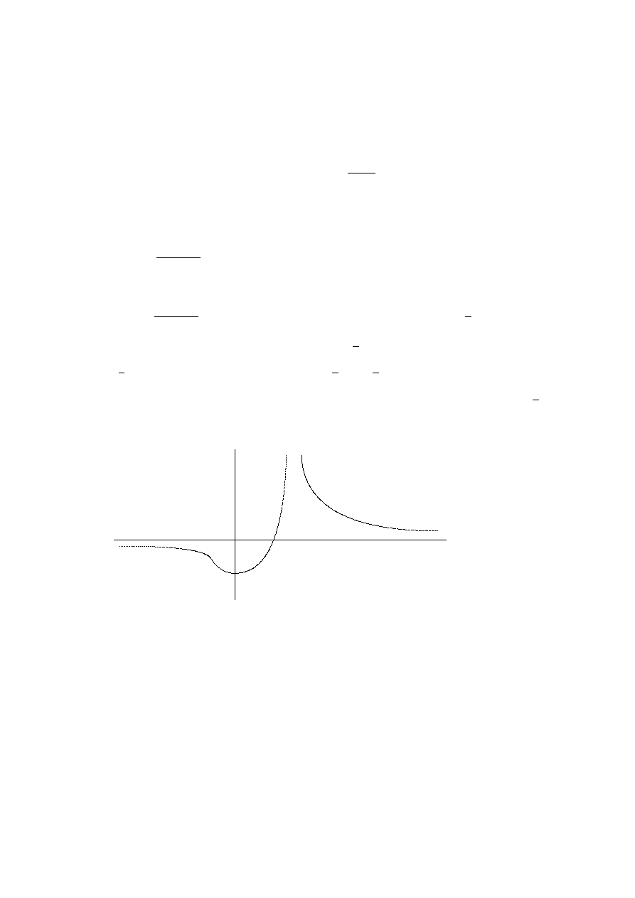
6. Find intervals in which f is convex (concave).
Definition 35 f is called convex (concave) at x
0
if f
00
(x
0
)
≥ 0 (f
00
(x
0
)
≤ 0), and
strictly convex (concave) if the inequalities are strict.
Example 50 Sketch the graph of the function y =
2x
−1
(x
−1)
2
.
a) y(x) is defined for x
∈ (−∞, 1) ∪ (1, +∞).
b) y(x) is continuous in (
−∞, 1) ∪ (1, +∞).
c) y(x)
→ 0 if x → ±∞, therefore y = 0 is the horizontal asymptote.
d) y(x)
→ ∞ if x → ±1, therefore x = 1 is the vertical asymptote.
e) y
0
(x) =
−
2x
(x
− 1)
3
. y
0
(x) is not defined at x = 1, it is positive if x
∈ (0, 1) (the
function is increasing) and negative if x
∈ (−∞, 0) ∪ (1, +∞) (the function is decreasing).
x = 0 is the unique extremum (minimum), y(0) =
−1.
f ) y
00
(x) = 2
2x
− 1
(x
− 1)
4
. It is not defined at x = 1, positive at x
∈ (−
1
2
, 1)
∪ (1, +∞)
(the function is convex) and negative at x
∈ (−∞, −
1
2
) ( the function is concave).
x =
−
1
2
is the unique point of inflection, y(
−
1
2
) =
−
8
9
.
g) Intersections with the axes are given by
x = 0
⇒ y(x) = −1,
y = 0
⇒ x =
1
2
.
Finally, the sketch of the graph looks like this:
6
6
-
y(x)
x
1/2
1
−1/2
−1
2.5
Integration (The Case of One Variable)
Definition 36 Let f (x) be a continuous function. The indefinite integral of f (denoted
by
R
f (x)dx) is defined as
Z
f (x)dx = F (x) + C,
where F (x) is such that F
0
(x) = f (x), and C is an arbitrary constant.
Rules of integration:
•
R
(af (x) + bg(x))dx = a
R
f (x)dx + b
R
g(x)dx, a, b are constants (linearity of the
integral);
29

•
R
f
0
(x)g(x)dx = f (x)g(x)
−
R
f (x)g
0
(x)dx
(integration by parts);
•
R
f (u(t))
du
dt
dt =
R
f (u)du
(integration by substitution).
Some special rules of integration:
R
f
0
(x)
f (x)
dx = ln
|f(x)| + C,
R
f
0
(x)e
f (x)
dx = e
f (x)
+ C
R
1
x
dx = ln
|x| + C,
R
x
a
dx =
x
a+1
a+1
+ C,
a
6= −1
R
e
x
dx = e
x
+ C,
R
a
x
dx =
a
x
ln a
+ C
a > 0
See any calculus reference-book for tables of integrals of basic functions.
Example 51
a)
Z
x
2
+ 2x + 1
x
dx =
Z
xdx +
Z
2dx +
Z
1
x
dx =
x
2
2
+ 2x + ln
|x| + C.
b)
Z
xe
−x
2
dx =
−
1
2
Z
(
−2x)e
−x
2
dx
(substitution z = x
2
)
=
−
1
2
Z
e
−z
dz =
−
e
−x
2
2
+ C.
c)
Z
xe
x
dx
(by parts, f (x) = x, g(x) = e
x
)
=
xe
x
−
Z
e
x
dx = xe
x
− e
x
+ C.
Definition 37 (the Newton-Leibniz formula).
The definite integral of a continuous function f is
Z
b
a
f (x)dx = F (x)
|
b
a
= F (b)
− F (a),
(2)
for F (x) such that F
0
(x) = f (x) for all x
∈ [a, b]
The indefinite integral is a function. The definite integral is a number!
4
!
We understand the definite integral in Riemann sense:
Given a partition a = x
0
< x
1
< . . . < x
n
= b and numbers ζ
i
∈ [x
i
, x
i+1
], i = 0, 1, . . . , n
− 1,
Z
b
a
f (x)dx =
lim
max
i
(x
i+1
−x
i
)
→0
n
−1
X
i=0
f (ζ
i
)(x
i+1
− x
i
).
Since every definite integral has a definite value, this value may be interpreted geo-
metrically to be a particular area under a given curve defined by y = f (x).
Note that if a curve lies below the x axis, this area will be negative.
4
!
Properties of definite integrals: For any arbitrary real numbers a, b, c, α, β
•
R
b
a
(αf (x) + βg(x))dx = α
R
b
a
f (x)dx + β
R
b
a
g(x)dx
•
R
b
a
f (x)dx =
−
R
a
b
f (x)dx
•
R
a
a
f (x)dx = 0
•
R
b
a
f (x)dx =
R
c
a
f (x)dx +
R
b
c
f (x)dx
• |
R
b
a
f (x)dx
| ≤
R
b
a
|f(x)|dx
•
R
b
a
f (x)g
0
(x)dx =
R
g(b)
g(a)
f (u)du,
u = g(x) (change of variable)
30

•
R
b
a
f (x)g
0
(x)dx = f (x)g(x)
|
b
a
−
R
b
a
f
0
(x)g(x)dx
Some more useful results: If λ is a real parameter,
•
d
dλ
R
b(λ)
a(λ)
f (x)dx = f (b(λ))b
0
(λ)
− f(a(λ))a
0
(λ)
In particular,
d
dx
R
x
a
f (t)dt = f (x)
If
R
b
a
d
dλ
f (x, λ)dx exists, then
•
d
dλ
R
b
a
f (x, λ)dx =
R
b
a
f
0
λ
(x, λ)dx
Example 52 We may apply this formula when we need to evaluate a definite in-
tegral, which can not be integrated in elementary functions. For instance, let us
find
I(λ) =
Z
1
0
xe
−λx
dx.
If we introduce another integral
J (λ) =
Z
1
0
e
−λx
dx =
−
e
−λx
λ
|
1
0
=
−
e
−λ
− 1
λ
,
then
I(λ) =
−
Z
1
0
d
dλ
e
−λx
dx =
−
dJ (λ)
dλ
=
1
− e
−λ
(1 + λ)
λ
2
.
We can combine the last two formulas to get:
• Leibniz’s formula:
d
dλ
Z
b(λ)
a(λ)
f (x, λ)dx = f (b(λ), λ)b
0
(λ)
− f(a(λ), λ)a
0
(λ) +
Z
b(λ)
a(λ)
f
0
λ
(x, λ)dx
Proposition 22 (Mean Value Theorem)
If f (x) is continuous in [a, b] then there exist at least one point c
∈ (a, b) such that
Z
b
a
f (x)dx = f (c)(b
− a).
Numerical methods of approximation the definite integrals:
a) The trapezoid formula: Denoting y
i
= f (a + i
b
−a
n
),
Z
b
a
f (x)dx
≈
b
− a
2n
(y
0
+ 2y
1
+ 2y
2
+ . . . + 2y
n
−1
+ y
n
),
n is an arbitrary integer number.
b) Simpson’s formula: Denoting y
i
= f (a + i
b
−a
2n
),
Z
b
a
f (x)dx
≈
b
− a
6n
(y
0
+ 4
n
X
i=1
y
2i
−1
+ 2
n
−1
X
i=1
y
2i
+ y
2n
).
Improper integrals are integrals of one of the following forms:
31

•
R
∞
a
f (x)dx = lim
b
→∞
R
b
a
f (x)dx or
R
b
−∞
f (x)dx = lim
a
→−∞
R
b
a
f (x)dx.
•
R
b
a
f (x)dx = lim
→0
R
b
a+
f (x)dx where lim
x
→a
f (x) =
∞.
•
R
b
a
f (x)dx = lim
→0
R
b
−
a
f (x)dx where lim
x
→b
f (x) =
∞.
If these limits exist, the improper integral is said to be convergent, otherwise it is
called divergent.
Example 53
Z
1
0
1
x
p
dx = lim
→0
+
Z
1
1
x
p
dx =
(
lim
→0
+
(ln 1
− ln ), p = 1
lim
→0
+
(
1
1
−p
−
1
−p
1
−p
), p
6= 1
Therefore the improper integral converges if p < 1 and diverges if p
≥ 1.
Economics Application 3 (The Optimal Subsidy and the Compensated Demand Curve)
Consider the consumer’s dual problem (recall that the dual to utility maximization is
expenditure minimization: we minimize the objective function M = p
x
x + p
y
y, subject to
the utility constraint U = U (x, y), where M is income level, x, y and p
x
, p
y
are quantities
and prices of two goods, respectively).
The solution to the expenditure-minimization problem under the utility constraint is
the budget line with income M
∗
, M
∗
(p
x
, p
y
) = p
x
x
∗
+ p
y
y
∗
.
If we hold utility and p
y
constant, due to Hotelling’s lemma
dM
∗
(p
x
)
dp
x
= x
∗
c
(p
x
),
where x
∗
c
(p
x
) is the income-compensated (or simply compensated) demand curve for good
x.
By rearranging terms, dM
∗
(p
x
) = x
∗
c
(p
x
)dp
x
, where dM
∗
is the optimal subsidy for
an infinitesimal change in price, we can “add up” a series of infinitesimal changes by
taking integral over those infinitesimal changes. Thus, if price increases from p
1
x
to p
2
x
,
the optimal subsidy S
∗
required to maintain a given level of utility would be the integral
over all the infinitesimal income changes as price changes:
S
∗
=
Z
p
2
x
p
1
x
x
∗
c
(p
x
)dp
x
.
For example, if p
1
x
= 1, p
2
x
= 4, x
∗
c
(p
x
) =
1
√
p
x
then
S
∗
=
Z
4
1
1
√
p
x
dp
x
= 2
√
p
x
|
4
1
= 2
· (2 − 1) = 2.
2.6
Functions of More than One Variable
Let us consider a function y = f (x
1
, x
2
, . . . , x
n
) where the variables x
i
, i = 1, 2, . . . , n
are all independent of one other, i.e. each varies without affecting others. The partial
derivative of y with respect to x
i
is defined as
∂y
∂x
i
= lim
∆x
i
→0
∆y
∆x
i
= lim
∆x
i
→0
f (x
1
, . . . , x
i
+ ∆x
i
, . . . , x
n
)
− f(x
1
, . . . , x
i
, . . . , x
n
)
∆x
i
for all i = 1, 2, . . . , n. If these limits exist, our function is differentiable with respect to all
arguments. Partial derivatives are often denoted with subscripts, e.g.
∂f
∂x
i
= f
x
i
(= f
0
x
i
).
32

Example 54 If y = 4x
3
1
+ x
1
x
2
+ ln x
2
then
∂y
∂x
1
= 12x
2
1
+ x
2
,
∂y
∂x
2
= x
1
+ 1/x
2
.
Definition 38 The total differential of a function f is defined as
dy =
∂f
∂x
1
dx
1
+
∂f
∂x
2
dx
2
+ . . . +
∂f
∂x
n
dx
n
.
The total differential can be also used as an approximation device.
For instance, if y = f (x
1
, x
2
) then by definition y
− y
0
= ∆f (x
0
1
, x
0
2
)
≈ df(x
0
1
, x
0
2
).
Therefore f (x
1
, x
2
)
≈ f(x
0
1
, x
0
2
)+df (x
0
1
, x
0
2
)
≈ f(x
0
1
, x
0
2
)+
∂f (x
0
1
, x
0
2
)
∂x
1
(x
1
−x
0
1
)+
∂f (x
0
1
, x
0
2
)
∂x
2
(x
2
−x
0
2
).
If y = f (x
1
, . . . , x
n
), x
i
= x
i
(t
1
, . . . , t
m
), i = 1, 2, . . . , n, then for all j = 1, 2, . . . , m
∂y
∂t
j
=
n
X
i=1
∂f (x
1
, . . . , x
n
)
∂x
i
∂x
i
∂t
j
.
This rule is called the chain rule.
Example 55 If z = f (x, y), x = u(t), y = v(t) then
dz
dt
=
∂f
∂x
dx
dt
+
∂f
∂y
dy
dt
.
(a special case of the chain rule)
Example 56 If z = f (x, y, t) where x = u(t), y = v(t) then
dz
dt
=
∂f
∂x
dx
dt
+
∂f
∂y
dy
dt
+
∂f
∂t
.
(dz/dt is sometimes called the total derivative).
Second order partial derivative of y = f (x
1
, . . . , x
n
) is defined as
∂
2
y
∂x
j
∂x
i
= f
x
i
x
j
(x
1
, . . . , x
n
) =
∂
∂x
j
f
x
i
(x
1
, . . . , x
n
),
i, j = 1, 2, . . . , n.
Proposition 23 (Schwarz’s Theorem or Young’s Theorem)
If at least one of the two partials is continuous, then
∂
2
f
∂x
j
∂x
i
=
∂
2
f
∂x
i
∂x
j
,
i, j = 1, 2, . . . , n.
Similar to the case of one variable, we can expand a function of several variables in a polynomial
form of Taylor series, using partial derivatives of higher order.
Definition 39 The second order total differential of a function y = f (x
1
, x
2
, . . . , x
n
) is
defined as
d
2
y = d(dy) =
n
X
i=1
n
X
j=1
∂
2
f
∂x
i
∂x
j
dx
i
dx
j
,
i, j = 1, 2, . . . , n.
Example 57 Let z = f (x, y) and f (x, y) satisfy the conditions of Schwarz’s theorem (i.e.
f
xy
= f
yx
). Then d
2
z = f
xx
dx
2
+ 2f
xy
dxdy + f
yy
dy
2
33

2.7
Unconstrained Optimization in the Case of More than One
Variable
Let z = f (x
1
, . . . , x
n
).
Definition 40 z has a stationary point at x
∗
= (x
∗
1
, . . . , x
∗
n
) if dz = 0 at x
∗
, i.e. all f
0
x
i
should vanish at x
∗
.
The conditions
f
0
x
i
(x
∗
) = 0, for all i = 1, 2, . . . , n
are called the first order necessary conditions (F.O.N.C.).
The second-order necessary condition (S.O.N.C.) requires sign semidefiniteness of the second order
total differential.
Definition 41 z = f (x
1
, . . . , x
n
) has a local maximum (minimum) at x
∗
= (x
∗
1
, . . . , x
∗
n
)
if f (x
∗
)
− f(x) ≥ 0(≤ 0) for all x in some neighborhood of x
∗
.
The second-order sufficient condition (S.O.C.):
x
∗
is a maximum (minimum) if d
2
z at x
∗
is negative definite (positive definite).
Recipe 11 – How to Check the Sign Definiteness of d
2
z:
Let us define the symmetric Hessian matrix H of second partial derivatives as
H =
∂
2
f
∂x
1
∂x
1
. . .
∂
2
f
∂x
1
∂x
n
..
.
..
.
∂
2
f
∂x
n
∂x
1
. . .
∂
2
f
∂x
n
∂x
n
.
Thus, the sign definiteness of d
2
z is equivalent to the sign definiteness of the quadratic
form H evaluated at x
∗
. We can apply either the principal minors test or the eigenvalue
test discussed in the previous chapter.
Example 58 Consider z = f (x, y). If the first order necessary conditions are met at x
∗
then
x
∗
is a (local)
(
minimum
maximum
)
if
(
f
00
xx
(x
∗
) > 0, f
00
xx
(x
∗
)f
00
yy
(x
∗
)
− (f
00
xy
(x
∗
))
2
> 0
f
00
xx
(x
∗
) < 0, f
00
xx
(x
∗
)f
00
yy
(x
∗
)
− (f
00
xy
(x
∗
))
2
> 0
)
.
If f
00
xx
(x
∗
)f
00
yy
(x
∗
)
− (f
00
xy
(x
∗
))
2
< 0, we identify a stationary point as a saddle point.
Note the sufficiency of this test. For instance, even if f
00
xx
(x
∗
)f
00
yy
(x
∗
)
− (f
00
xy
(x
∗
))
2
= 0,
we still may have an extremum at (x
∗
).
4
!
Example 59 (Classification of Stationary Points of a C
(2)
-Function
3
of n Variables)
If x
∗
= (x
∗
1
, . . . , x
∗
n
) is a stationary point of f (x
1
, . . . , x
n
) and if
|H
k
(x
∗
)
| is the follow-
ing determinant evaluated at x
∗
,
|H
k
| = det
∂
2
f
∂x
1
∂x
1
. . .
∂
2
f
∂x
1
∂x
k
..
.
..
.
∂
2
f
∂x
k
∂x
1
. . .
∂
2
f
∂x
k
∂x
k
,
k = 1, 2, . . . , n
then
3
Recall that C
(2)
means ‘twice continuously differentiable’.
34

a) if (
−1)
k
|H
k
(x
∗
)
| > 0, k = 1, 2, . . . , n, then x
∗
is a local maximum;
b) if
|H
k
(x
∗
)
| > 0, k = 1, 2, . . . , n, then x
∗
is a local minimum;
c) if
|H
n
(x
∗
)
| 6= 0 and neither of the two conditions above is satisfied, then x
∗
is a
saddle point.
Example 60 Let us find the extrema of the function z(x, y) = x
3
− 8y
3
+ 6xy + 1.
F.O.N.C.:
z
x
= 3(x
2
+ 2y) = 0,
z
y
= 6(
−4y
2
+ x) = 0.
Solving F.O.N.C. for x, y we obtain two stationary points:
x = y = 0 and x = 1, y =
−1/2.
S.O.C.: The Hessian matrices evaluated at stationary points are
H
|
(0,0)
=
6x
6
6
−48y
!
(0,0)
=
0 6
6 0
!
,
H
|
(1,
−1/2)
=
6
6
6 24
!
,
therefore (0, 0) is a saddle point, (1,
−1/2) is a local minimum.
2.8
The Implicit Function Theorem
Proposition 24 (The Two-Dimensional Case)
If F (x, y)
∈ C
(k)
in a set D (i.e. F is k times continuously differentiable at any
point in D) and (x
0
, y
0
) is an interior point of D, F (x
0
, y
0
) = c (c is constant) and
F
0
y
(x
0
, y
0
)
6= 0 then the equation F (x, y) = c defines y as a C
(k)
-function of x in some
neighborhood of (x
0
, y
0
), i.e. y = ψ(x) and
dy
dx
=
−
F
0
x
(x, y)
F
0
y
(x, y)
.
Example 61 Let consider the function
1
− e
−ax
1 + e
ax
, where a is a parameter, a > 1.
What happens to the extremum value of x if a increases by a small number?
To answer this question, first write down the F.O.N.C. for a stationary point:
f
0
x
=
a(e
−ax
− e
ax
+ 2)
((1 + e
ax
)
2
= 0.
If this expression vanishes at, say, x = x
∗
, we can apply the implicit function theorem to
the F.O.N.C. and obtain
dx
da
=
−
∂(e
−ax
− e
ax
+ 2)/∂a
∂(e
−ax
− e
ax
+ 2)/∂x
=
−
x
a
< 0
in some neighborhood of (x
∗
, a). The negativity of the derivative is due to the fact that x
∗
is positive, therefore, every x in a small neighborhood of x
∗
should be positive as well.
35

Let us formulate the general case of the implicit function theorem.
Consider the system of m equations with n exogenous variables, x
1
, . . . , x
n
, and m
endogenous variables, y
1
, . . . , y
m
:
f
1
(x
1
, . . . , x
n
, y
1
, . . . , y
m
) = 0
f
2
(x
1
, . . . , x
n
, y
1
, . . . , y
m
) = 0
. . . . . . . . .
f
m
(x
1
, . . . , x
n
, y
1
, . . . , y
m
) = 0
(3)
Our objective is to find
∂y
j
∂x
i
, i = 1, . . . , n, j = 1, . . . , m.
If we take the total differentials of all f
j
, we get
∂f
1
∂y
1
dy
1
+ . . . +
∂f
1
∂y
m
dy
m
=
−
∂f
1
∂x
1
dx
1
+ . . . +
∂f
1
∂x
n
dx
n
!
,
. . .
∂f
m
∂y
1
dy
1
+ . . . +
∂f
m
∂y
m
dy
m
=
−
∂f
m
∂x
1
dx
1
+ . . . +
∂f
m
∂x
n
dx
n
!
.
Now allow only x
i
to vary (i.e. dx
i
6= 0, dx
l
= 0, l = 1, 2, . . . , i
−1, i+1, . . . , n) and divide
each remaining term in the system above by dx
i
. Thus we arrive at the following linear
system with respect to
∂y
1
∂x
i
, . . .
∂y
m
∂x
i
(note, that in fact dy
1
/dx
i
, . . . , dy
m
/dx
i
should be
interpreted as partial derivatives with respect to x
i
since we allow only x
i
to vary, holding
constant all other x
l
):
∂f
1
∂y
1
∂y
1
∂x
i
+ . . . +
∂f
1
∂y
m
∂y
m
∂x
i
=
−
∂f
1
∂x
i
,
. . .
∂f
m
∂y
1
∂y
1
∂x
i
+ . . . +
∂f
m
∂y
m
∂y
m
∂x
i
=
−
∂f
m
∂x
i
,
which can be solved for
∂y
1
∂x
i
, . . .
∂y
m
∂x
i
by, say, Cramer’s rule or by the inverse matrix
method.
Let define the Jacobian matrix of f
1
, . . . , f
m
with respect to y
1
, . . . , y
m
as
J =
∂f
1
∂y
1
. . .
∂f
1
∂y
m
..
.
. ..
..
.
∂f
m
∂y
1
. . .
∂f
m
∂y
m
.
Given the definition of Jacobian, we are in a position to formulate the general result:
Proposition 25 (The General Implicit Function Theorem)
Suppose f
1
, . . . , f
m
are C
(k)
-functions in a set D
⊂R
n+m
.
Let (x
∗
, y
∗
) = (x
∗
1
, . . . , x
∗
n
, y
∗
1
, . . . , y
∗
m
) be a solution to (3) in the interior of A.
36

Suppose also that det(
J ) does not vanish at (x
∗
, y
∗
). Then (3) defines y
1
, . . . , y
m
as
C
(k)
-functions of x
1
, . . . , x
n
in some neighborhood of (x
∗
, y
∗
) and in that neighborhood, for
j = 1, 2, . . . , n,
∂y
1
∂x
j
..
.
∂y
m
∂x
j
=
−J
−1
·
∂f
1
∂x
j
..
.
∂f
m
∂x
j
.
Example 62 Given the system of two equations x
2
+ y
2
= z
2
/2 and x + y + z = 2, find
x
0
= x
0
(z), y
0
= y
0
(z) in the neighborhood of the point (1,
−1, 2).
In this setup, f
1
(x, y, z) = x
2
+ y
2
− z
2
/2, f
2
(x, y, z) = x + y + z
− 2, f
1
, f
2
∈ C
∞
(R
3
),
f
1
(1,
−1, 2) = f
2
(1,
−1, 2) = 0, and at (1, −1, 2)
det(
J ) = det
∂f
1
∂x
∂f
1
∂y
∂f
2
∂x
∂f
2
∂y
= det
2x 2y
1
1
!
(1,
−1,2)
= det
2
−2
1
1
!
= 4
6= 0.
Therefore the conditions of the implicit function theorem are satisfied and
dx
dz
dy
dz
!
=
−
1
2x
− 2y
1
−2y
−1
2x
!
−z
1
!
=
⇒
dx
dz
=
z+2y
2x
−2y
dy
dz
=
−
z+2x
2x
−2y
The Jacobian matrix can be also applied to test whether functional (linear or nonlinear) dependence
exists among a set of n functions in n variables. More precisely, if we have n functions of n variables
g
i
= g
i
(x
1
, . . . , x
n
), i = 1, 2, . . . , n, then the determinant of the Jacobian matrix of g
1
, . . . , f
n
with
respect to x
1
, . . . , x
m
will be identically zero for all values of x
1
, . . . , x
n
if and only if the n functions
g
1
, . . . , g
n
are functionally (linearly or nonlinearly) dependent.
Economics Application 4 (The Profit-Maximizing Firm)
Consider that a firm has the profit function F (l, k) = pf (l, k)
− wl − rk where f is
the firm’s (neoclassical) production function, p is the price of output, l,k are the amount
of labor and capital employed by the firm (in units of output), w is the real wage and r
is the real rental price of capital. The firm takes p, w and r as given. Assume that the
Hessian matrix of f is negative definite.
a) Show that if the wage increases by a small amount, then the firm decides to employ
less labor.
b) Show that if the wage increases by a small amount and the firm is constrained to
maintain the same amount of capital k
0
, then the firm will reduce l by less than it does in
part a).
Solution.
a) The firm’s objective is to choose l and k so that it maximizes its profits. The
first-order conditions for maximization are:
(
p
∂f
∂l
(l, k)
− w = 0
p
∂f
∂k
(l, k)
− r
= 0
or,
(
F
1
(l, k; w) = 0
F
2
(l, k; r)
= 0
The Jacobian of this system of equations is:
|J| =
∂F
1
∂l
∂F
1
∂k
∂F
2
∂l
∂F
2
∂k
= p
2
f
11
(l, k) f
12
(l, k)
f
12
(l, k) f
22
(l, k)
= p
2
|H| > 0.
37

where f
ij
is the second-order partial derivative of f with respect to the jth and the ith
arguments and
|H| is the Hessian of f. The fact that H is negative definite means that
f
11
< 0 and
|H| > 0 (which also implies f
22
< 0).
Since
|J| 6= 0 the implicit-function theorem can be applied; thus, l and k are implicit
functions of w. The first-order partial derivative of l with respect to w is:
∂l
∂w
=
−
−1 pf
12
(l, k)
0
pf
22
(l, k)
|J|
=
f
22
(l, k)
p
|H|
< 0.
Thus, the optimal l falls in response to a small increase in w.
b) If the firm’s amount of capital is fixed at k
0
, the profit function is F (l) = pf (l, k
0
)
−
wl
− rk
0
and the first-order condition is
p
∂f
∂l
(l, k
0
)
− w = 0.
Since f
11
6= 0, the above condition defines l as an implicit function of w. Taking the
derivative of the F.O.C. with respect to l, we have:
pf
11
(l, k
0
)
∂l
∂w
= 1 or
∂l
∂w
=
1
pf
11
(l, k
0
)
.
This change in l is smaller in absolute value than the change in l in part a) since
f
22
(l, k
0
)
p
|H|
<
1
pf
11
(l, k
0
)
(Note that both ratios are negative.)
For another economic application see the section ‘Constrained Optimization’.
2.9
Concavity, Convexity, Quasiconcavity and Quasiconvexity
Definition 42 A function z = f (x
1
, . . . , x
n
) is concave if and only if for any pair of
distinct points u = (u
1
, . . . , u
n
) and v = (v
1
, . . . , v
n
) in the domain of f and for any
θ
∈ (0, 1)
θf (u) + (1
− θ)f(v) ≤ f(θu + (1 − θ)v)
and convex if and only if
θf (u) + (1
− θ)f(v) ≥ f(θu + (1 − θ)v).
If f is differentiable, an alternative definition of concavity (or convexity) is
f (v)
≤ f(u) +
n
X
i=1
f
0
x
i
(u)(v
i
− u
i
)
(or f (v)
≥ f(u) +
n
X
i=1
f
0
x
i
(u)(v
i
− u
i
)).
If we change weak inequalities
≤ and ≥ to strict inequalities, we will get the definition
of strict concavity and strict convexity, respectively.
38

Some useful results:
• The sum of concave (or convex) functions is a concave (or convex) function. If,
additionally, at least one of these functions is strictly concave (or convex), the sum
is also strictly concave (or convex).
• If f(x) is a (strictly) concave function then −f(x) is a (strictly) convex function
and vise versa.
Recipe 12 – How to Check Concavity (or Convexity):
A twice continuously differentiable function z = f (x
1
, . . . , x
n
) is concave (or convex)
if and only if d
2
z is everywhere negative (or positive) semidefinite.
z = f (x
1
, . . . , x
n
) is strictly concave (or strictly convex) if (but not only if ) d
2
z is
everywhere negative (or positive) definite.
Again, any test for the sign definiteness of a symmetric quadratic form is applicable.
Example 63 z(xy) = x
2
+ xy + y
2
is strictly convex.
The conditions for concavity and convexity are necessary and sufficient, while those
for strict concavity (strict convexity) are only sufficient.
4
!
Definition 43 A set S in R
n
is convex if for any x, y
∈ S and any θ ∈ [0, 1] the linear
combination θx + (1
− θ)y ∈ S.
Definition 44 A function z = f (x
1
, . . . , x
n
) is quasiconcave if and only if for any pair
of distinct points u = (u
1
, . . . , u
n
) and v = (v
1
, . . . , v
n
) in the convex domain of f and for
any θ
∈ (0, 1)
f (v)
≥ f(u) =⇒ f(θu + (1 − θ)v) ≥ f(u)
and quasiconvex if and only if
f (v)
≥ f(u) =⇒ f(θu + (1 − θ)v) ≤ f(v).
If f is differentiable, an alternative definition of quasiconcavity (quasiconvexity) is
f (v)
≥ f(u) =⇒
n
X
i=1
f
0
x
i
(u)(v
i
− u
i
)
≥ 0 (f(v) ≥ f(u) =⇒
n
X
i=1
f
0
x
i
(v)(v
i
− u
i
)
≥ 0).
A change of weak inequalities
≤ and ≥ on the right to strict inequalities gives us the
definitions of strict quasiconcavity and strict quasiconvexity, respectively.
Example 64 The function z(x, y) = xy, x, y
≥ 0 is quasiconcave.
Note that any convex (concave) function is quasiconvex (quasiconcave), but not vice
versa.
4
!
39

2.10
Appendix: Matrix Derivatives
Matrix derivatives play an important role in economic analysis, especially in econometrics.

If A is [n
× n] non-singular matrix, the derivative of its determinant with respect to
A is given by
∂
∂A
(det(A)) = (C
ij
),
where (C
ij
) is the matrix of cofactors of A.
Example 65 (Matrix Derivatives in Econometrics: How to Find the Least Squares Es-
timator in a Multiple Regression Model)
Consider the multiple regression model:
y = Xβ +
where n
× 1 vector y is the dependent variable, X is a n × k matrix of k explanatory
variables with rank(X) = k, β is a k
× 1 vector of coefficients which are to be estimated
and is a n
× 1 vector of disturbances. We assume that the matrices of observations
X and y are given.
Our goal is to find an estimator b for β using the least squares method. The least
squares estimator of β is a vector b, which minimizes the expression
E(b) = (y
− Xb)
0
(y
− Xb) = y
0
y
− y
0
Xb
− b
0
X
0
y + b
0
X
0
Xb.
The first-order condition for extremum is:
dE(b)
db
= 0.
To obtain the first order conditions we use the following formulas:
•
d(a
0
b)
db
= a,
•
d(b
0
a)
db
= a,
•
d(M b)
db
= M
0
,
•
d(b
0
M b)
db
= (M + M
0
)b,
where a, b are k
× 1 vectors and M is a k × k matrix.
Using these formulas we obtain:
dE(b)
db
=
−2X
0
y + 2X
0
Xb
and the first-order condition implies:
X
0
Xb = X
0
y
41

or
b = (X
0
X)
−1
X
0
y
On the other hand, by the third derivation rule above, we have:
d
2
E(b)
db
2
= (2X
0
X)
0
= 2X
0
X.
To check whether the solution b is indeed a minimum, we need to prove the positive
definiteness of the matrix X
0
X.
First, notice that X
0
X is a symmetric matrix. The symmetry is obvious:
(X
0
X)
0
= X
0
X.
To prove positive definiteness, we take an arbitrary k
× 1 vector z, z 6= 0 and check the
following quadratic form:
z
0
(X
0
X)z = (Xz)
0
Xz.
The assumptions rank(X) = k and z
6= 0 imply Xz 6= 0. It follows that (Xz)
0
Xz > 0 for
any z
6= 0 or, equivalently, z
0
X
0
Xz > 0 for any z
6= 0, which means that (by definition)
X
0
X is positive definite.
Further Reading:
• Bartle, R.G. The Elements of Real Analysis.
• Edwards, C.N and D.E.Penny. Calculus and Analytical Geomethry.
• Greene, W.H. Econometric Analysis.
• Rudin, W. Principles of Mathematical Analysis.
42

3
Constrained Optimization
3.1
Optimization with Equality Constraints
Consider the problem
4
:
extremize f (x
1
, . . . , x
n
)
(4)
subject to g
j
(x
1
, . . . , x
n
) = b
j
,
j = 1, 2, . . . , m < n.
f is called the objective function, g
1
, g
2
, . . . , g
m
are the constraint functions, b
1
, b
2
, . . . , b
m
are the constraint constants. The difference n
− m is the number of degrees of freedom of
the problem.
Note that n is strictly greater than m.
4
!
If it is possible to explicitly express (from the constraint functions) m independent
variables as functions of the other n
− m independent variables, we can eliminate m
variables in the objective function, thus the initial problem will be reduced to the uncon-
strained optimization problem with respect to n
− m variables. However, in many cases
it is not technically feasible to explicitly express one variable as function of the others.
Instead of the substitution and elimination method, we may resort to the easy-to-use
and well-defined method of Lagrange multipliers.
Let f and g
1
, . . . , g
m
be C
(1)
-functions and the Jacobian
J = (
∂g
j
∂x
i
), i = 1, 2, . . . , n, j =
1, 2, . . . , m have the full rank, i.e.rank(
J ) = m. We introduce the Lagrangian function as
L(x
1
, . . . , x
n
, λ
1
, . . . , λ
m
) = f (x
1
, . . . , x
n
) +
m
X
j=1
λ
j
(b
j
− g
j
(x
1
, . . . , x
n
)),
where λ
1
, λ
2
, . . . , λ
m
are constant (Lagrange multipliers).
Recipe 13 – What are the Necessary Conditions for the Solution of (4)?
Equate all partials of L with respect to x
1
, . . . , x
n
, λ
1
, . . . , λ
m
to zero:
∂L(x
1
, . . . , x
n
, λ
1
, . . . , λ
m
)
∂x
i
=
∂f (x
1
, . . . , x
n
)
∂x
i
−
m
X
j=1
λ
j
∂g
j
(x
1
, . . . , x
n
)
∂x
i
= 0,
i = 1, 2, . . . , n,
∂L(x
1
, . . . , x
n
, λ
1
, . . . , λ
m
)
∂λ
j
= b
j
− g
j
(x
1
, . . . , x
n
) = 0,
j = 1, 2, . . . , m.
Solve these equations for x
1
, . . . , x
n
and λ
1
, . . . , λ
m
.
In the end we will get a set of stationary points of the Lagrangian. If x
∗
= (x
∗
1
, . . . , x
∗
n
)
is a solution of (4), it should be a stationary point of L.
It is important that rank(
J ) = m, and the functions are continuously differentiable.
4
!
Example 66 This example shows that the Lagrange-multiplier method does not always
provide the solution to an optimization problem. Consider the problem:
min x
2
+ y
2
subject to (x
− 1)
3
− y
2
= 0.
4
“Extremize” means to find either the minimum or the maximum of the objective function f .
43

Notice that the solution to this problem is (1, 0). The restriction (x
− 1)
3
= y
2
implies
x
≥ 1. If x = 1, then y = 0 and x
2
+ y
2
= 1. If x > 1, then y > 0 and x
2
+ y
2
> 1. Thus,
the minimum of x
2
+ y
2
is attained for (1, 0).
The Lagrangian function is
L = x
2
+ y
2
− λ[(x − 1)
3
− y
2
]
The first-order conditions are
∂
L
∂x
= 0
∂
L
∂y
= 0
∂
L
∂λ
= 0
or
2x
− 3λ(x − 1)
2
= 0
2y + 2λy
= 0
(x
− 1)
3
− y
2
= 0
Clearly, the first equation is not satisfied for x = 1. Thus, the Lagrange-multiplier
method fails to detect the solution (1, 0).
If we need to check whether a stationary point is a maximum or minimum, the following
local sufficient conditions can be applied:
Proposition 26 Let us introduce a bordered Hessian
| ¯
H
r
| as
| ¯
H
r
| = det
0
. . .
0
∂g
1
∂x
1
. . .
∂g
1
∂x
r
..
.
. ..
..
.
..
.
. ..
..
.
0
. . .
0
∂g
m
∂x
1
. . .
∂g
m
∂x
r
∂g
1
∂x
1
. . .
∂g
m
∂x
1
∂
2
L
∂x
1
∂x
1
. . .
∂
2
L
∂x
1
∂x
r
..
.
. ..
..
.
..
.
. ..
..
.
∂g
1
∂x
r
. . .
∂g
m
∂x
r
∂
2
L
∂x
r
∂x
1
. . .
∂
2
L
∂x
r
∂x
r
,
r = 1, 2, . . . , n.
Let f and g
1
, . . . , g
m
are C
(2)
-functions and let x
∗
satisfy the necessary conditions for the
problem (4). Let
| ¯
H
r
(x
∗
)
| be the bordered Hessian determinant evaluated at x
∗
. Then
• if (−1)
m
| ¯
H
r
(x
∗
)
| > 0, r = m + 1, . . . , n, then x
∗
is a local minimum point for the
problem (4).
• if (−1)
r
| ¯
H
r
(x
∗
)
| > 0, r = m + 1, . . . , n, then x
∗
is a local maximum point for the
problem (4).
Example 67 (Local Second-Order Conditions for the Case with one Constraint)
Suppose that x
∗
= (x
∗
1
, . . . , x
∗
n
) satisfies the necessary conditions for the problem
max(min)f (x
1
, . . . , x
n
) subject to g(x
1
, . . . , g
n
) = b,
i.e. all partial derivatives of the Lagrangian are zero at x
∗
. Define
| ¯
H
r
| = det
0
∂g
∂x
1
. . .
∂g
∂x
r
∂g
∂x
1
∂
2
L
∂x
1
∂x
1
. . .
∂
2
L
∂x
1
∂x
r
..
.
..
.
. ..
..
.
∂g
∂x
r
∂
2
L
∂x
r
∂x
1
. . .
∂
2
L
∂x
r
∂x
r
,
r = 1, 2, . . . , n.
Let
| ¯
H
r
(x
∗
)
| be | ¯
H
r
| evaluated at x
∗
. Then
44

• x
∗
is a local minimum point of f subject to the given constraint if
| ¯
H
r
(x
∗
)
| < 0 for
all r = 2, . . . , n.
• x
∗
is a local maximum point of f subject to the given constraint if (
−1)
r
| ¯
H
r
(x
∗
)
| > 0
for all r = 2, . . . , n.
Economics Application 5 (Utility Maximization)
In order to illustrate how the Lagrange-multiplier method can be applied, let us consider
the following optimization problem:
The preferences of a consumer over two goods x and y are given by the utility function
U (x, y) = (x + 1)(y + 1) = xy + x + y + 1.
The prices of goods x and y are 1 and 2, respectively, and the consumer’s income is 30.
What bundle of goods will the consumer choose?
The consumer’s budget constraint is x + 2y
≤ 30 which, together with the conditions
x
≥ 0 and y ≥ 0, determines his budget set (the set of all affordable bundles of goods).
He will choose the bundle from his budget set that maximizes his utility. Since U (x, y) is
an increasing function in both x and y (over the domain x
≥ 0 and y ≥ 0), the budget
constraint should be satisfied with equality. The consumer’s optimization problem can be
stated as follows:
max U (x, y)
subject to x + 2y = 30.
The Lagrangian function is
L = U (x, y)
− λ(x + 2y − 30)
= xy + x + y + 1
− λ(x + 2y − 30).
The first-order necessary conditions are
∂L
∂x
= 0
∂
L
∂y
= 0
∂
L
∂z
= 0
or
y + 1
− λ
= 0
x + 1
− 2λ
= 0
x + 2y
− 30 = 0
From the first equation, we get λ = y + 1; substituting y + 1 for λ in the second equation,
we obtain x
− 2y − 1 = 0. This condition and the third condition above lead to x =
31
2
,
y =
29
4
.
To check whether this solution really maximizes the objective function, let us apply the
second order sufficient conditions.
The second-order conditions involve the bordered Hessian:
det ¯
H =
0 1 2
1 0 1
2 1 0
= 4 > 0.
Thus, (x =
31
2
, y =
29
4
) is indeed a maximum and represents the bundle demanded by the
consumer.
45

Economics Application 6 (Applications of the Implicit-Function Theorem)
Consider the problem of maximizing the function f (x, y) = ax + y subject to the
constraint x
2
+ ay
2
= 1 where x > 0, y > 0 and a is a positive parameter. Given that this
problem has a solution, find how the optimal values of x and y change if a increases by a
very small amount.
Solution:
Differentiation of the Lagrangian function L = ax + y
− λ(x
2
+ ay
2
− 1) with respect
to x, y, λ gives the first-order conditions:
a
− 2λx
= 0
1
− 2aλy
= 0
x
2
+ ay
2
− 1 = 0
or,
F
1
(x, λ; a) = 0
F
2
(y, λ; a) = 0
F
3
(x, y; a)
= 0
(5)
The Jacobian of this system of three equations is:
J =
∂F
1
∂x
∂F
1
∂y
∂F
1
∂λ
∂F
2
∂x
∂F
2
∂y
∂F
2
∂λ
∂F
3
∂x
∂F
3
∂y
∂F
3
∂λ
=
−2λ
0
−2x
0
−2aλ −2ay
2x
2ay
0
,
|J| = −8aλ(x
2
+ ay
2
) =
−8aλ.
From the first F.O.C. we can see that λ > 0, thus
|J| < 0 at the optimal point. Therefore,
in a neighborhood of the optimal solution, given by the system (5), the conditions of the
implicit-function theorem are met, and in this neighborhood x and y can be expressed as
functions of a.
The first-order partial derivatives of x and y with respect to a are evaluated as:
∂x
∂a
=
−
∂F
1
∂a
∂F
1
∂y
∂F
1
∂λ
∂F
2
∂a
∂F
2
∂y
∂F
2
∂λ
∂F
3
∂a
∂F
3
∂y
∂F
3
∂λ
|J|
=
−
1λ
0
−2x
−2λy −2aλ −2ay
y
2
2ay
0
|J|
=
=
4ay
2
(λx + a)
8aλ
=
3xy
2
2
> 0.
∂y
∂a
=
−
∂F
1
∂x
∂F
1
∂a
∂F
1
∂λ
∂F
2
∂x
∂F
2
∂a
∂F
2
∂λ
∂F
3
∂x
∂F
3
∂a
∂F
3
∂λ
|J|
=
−
−2λ
1
−2x
0
−2λy −2ay
2x
y
2
0
|J|
=
=
−
−4xy(λx + a) − 4λy(x
2
+ ay
2
)
−8aλ
=
−
3xy
4λ
+
y
2a
< 0.
In conclusion, a small increase in a will lead to a rise in the optimal x and a fall in
the optimal y.
Proposition 27 Suppose that f and g
1
, . . . , g
m
are defined on an open convex set S
⊂R
n
.
Let x
∗
be a stationary point of the Lagrangian. Then,
• if the Lagrangian is concave, x
∗
maximizes (4);
• if the Lagrangian is convex, x
∗
minimizes (4).
46

3.2
The Case of Inequality Constraints
Classical methods of optimization (the method of Lagrange multipliers) deal with opti-
mization problems with equality constraints in the form of g(x
1
, . . . , x
n
) = c. Nonclassical
optimization, also known as mathematical programming, tackles problems with inequality
constraints like g(x
1
, . . . , x
n
)
≤ c.
Mathematical programming includes linear programming and nonlinear programming.
In linear programming, the objective function and all inequality constraints are linear.
When either the objective function or an inequality constraint is nonlinear, we face a
problem of nonlinear programming.
In the following, we restrict our attention to non-linear programming. A problem of
linear programming – also called a linear program – is discussed in the Appendix to this
chapter.
3.2.1
Non-Linear Programming
The nonlinear programming problem is that of choosing nonnegative values of certain
variables so as to maximize or minimize a given (non-linear) function subject to a given
set of (non-linear) inequality constraints.
The nonlinear programming maximum problem is
max f (x
1
, . . . , x
n
)
(6)
subject to g
i
(x
1
, . . . , x
n
)
≤ b
i
,
i = 1, 2, . . . , m.
x
1
≥ 0, . . . , x
n
≥ 0
Similarly, the minimization problem is
min f (x
1
, . . . , x
n
)
subject to g
i
(x
1
, . . . , x
n
)
≥ b
i
,
i = 1, 2, . . . , m.
x
1
≥ 0, . . . , x
n
≥ 0
First, note that there are no restrictions on the relative size of m and n, unlike the case
of equality constraints. Second, note that the direction of the inequalities (
≤ or ≥) at the
constraints is only a convention, because the inequality g
i
≤ b
i
can be easily converted to
the
≥ inequality by multiplying it by –1, yielding −g
i
≥ −b
i
. Third, note that an equality
constraint, say g
k
= b
k
, can be replaced by the two inequality constraints, g
k
≤ b
k
and
−g
k
≤ −b
k
.
4
!
Definition 45 A constraint g
j
≤ b
j
is called binding (or active) at x
0
= (x
0
1
, . . . , x
0
n
) if
g
j
(x
0
) = b
j
.
Example 68 The following is an example of a nonlinear program:
Max π = x
1
(10
− x
1
) + x
2
(20
− x
2
)
subject to 5x
1
+ 3x
2
≤ 40
x
1
≤ 5
x
2
≤ 10
x
1
≥ 0, x
2
≥ 0.
47

Example 69 (How to Solve a Nonlinear Program Graphically)
An intuitive way to understand a low-dimensional non-linear program is to represent
the feasible set and the objective function graphically.
For instance, we may try to represent graphically the optimization problem from Ex-
ample 68, which can be re-written as
Max π = 125
− (x
1
− 5)
2
− (x
2
− 10)
2
subject to 5x
1
+ 3x
2
≤ 40
x
1
≤ 5
x
2
≤ 10
x
1
≥ 0, x
2
≥ 0;
or
Min C = (x
1
− 5)
2
+ (x
2
− 10)
2
subject to 5x
1
+ 3x
2
≤ 40
x
1
≤ 5
x
2
≤ 10
x
1
≥ 0, x
2
≥ 0.
Region OABCD below shows the feasible set of the nonlinear program.
5
10
5
2
"!
#
O
AB
C
D
-
p
6
x
2
x
1
Feasible Set
The value of the objective function can be interpreted as the square of the distance
from the point (5, 10) to the point (x
1
, x
2
). Thus, the nonlinear program requires us to
find the point in the feasible region which minimizes the distance to the point (5, 10).
As can be seen in the figure above, the optimal point (x
∗
1
, x
∗
2
) lies on the line 5x
1
+3x
2
=
40 and it is also the tangency point with a circle centered at (5, 10). These two conditions
are sufficient to determine the optimal solution.
Consider (x
1
− 5)
2
+ (x
2
− 10)
2
− C = 0. From the implicit-function theorem, we have
dx
2
dx
1
=
−
x
1
− 5
x
2
− 10
.
Thus, the tangent to the circle centered at (5, 10) which has the slope
−
5
3
is given by the
equation
−
5
3
=
−
x
1
− 5
x
2
− 10
or
3x
1
− 5x
2
+ 35 = 0.
48

Solving the system of equations
(
5x
1
+ 3x
2
= 40
3x
1
− 5x
2
=
−35
we find the optimal solution (x
∗
1
, x
∗
2
) = (
95
34
,
295
34
).
3.2.2
Kuhn-Tucker Conditions
For the purpose of ruling out certain irregularities on the boundary of the feasible set, a
restriction on the constrained functions is imposed. This restriction is called the constraint
qualification.
Definition 46 Let ¯
x = (x
1
, . . . , x
n
) be a point on the boundary of the feasible region of a
nonlinear program.
i) A vector dx = (dx
1
, . . . , dx
n
)is a test vector of ¯
x if it satisfies the conditions
• ¯
x
j
= 0 =
⇒ dx
j
≥ 0;
• g
i
(¯
x) = r
i
=
⇒ dg
i
(¯
x)
≤ (≥)0 for a maximization (minimization) program.
ii) A qualifying arc for a test vector of ¯
x is an arc with the point of origin ¯
x, contained
entirely in the feasible region and tangent to the test vector.
iii) The constraint qualification is a condition which requires that, for any boundary
point ¯
x of the feasible region and for any test vector of ¯
x, there exist a qualifying
arc for that test vector.
The constraint qualification condition is often imposed in the following way:
the gradients at x
∗
of those g
j
-constraints which are binding at x
∗
are linearly independent.
Assume that the constraint qualification condition is satisfied and the functions in
(6) are differentiable. If x
∗
is the optimal solution to (6), it should satisfy the following
conditions (the Kuhn-Tucker necessary maximum conditions or KT conditions):
∂L
∂x
i
≤ 0, x
i
≥ 0 and x
i
∂L
∂x
i
= 0,
i = 1, . . . , n,
∂L
∂λ
j
≥ 0, λ
j
≥ 0 and λ
j
∂L
∂λ
j
= 0,
j = 1, . . . , m
where
L(x
1
, . . . , x
n
, λ
1
, . . . , λ
m
) = f (x
1
, . . . , x
n
) +
m
X
j
−1
λ
j
(b
j
− g
j
(x
1
, . . . , x
n
))
is the Lagrangian function of a non-linear program.
The minimization version of Kuhn-Tucker necessary conditions is
∂L
∂x
i
≥ 0, x
i
≥ 0 and x
i
∂L
∂x
i
= 0,
i = 1, . . . , n,
49

∂L
∂λ
j
≤ 0, λ
j
≥ 0 and λ
j
∂L
∂λ
j
= 0,
j = 1, . . . , m
Note that, in general, the KT conditions are neither necessary nor sufficient for a
local optimum. However, if certain assumptions are satisfied, the KT conditions become
necessary and even sufficient.
4
!
Example 70 The Lagrangian function of the nonlinear program in Example 68 is:
L = x
1
(10
− x
1
) + x
2
(20
− x
2
)
− λ
1
(5x
1
+ 3x
2
− 40) − λ
2
(x
1
− 5) − λ
3
(x
2
− 10).
The KT conditions are:
∂L
∂x
1
= 10
− 2x
1
− 5λ
1
− λ
2
≤ 0
∂L
∂x
2
= 20
− 2x
2
− 3λ
1
− λ
3
≤ 0
∂L
∂λ
1
=
−(5x
1
+ 3x
2
− 40) ≥ 0
∂L
∂λ
2
=
−(x
1
− 5) ≥ 0
∂L
∂λ
3
=
−(x
2
− 10) ≥ 0
x
1
≥ 0, x
2
≥ 0
λ
1
≥ 0, λ
2
≥ 0, λ
3
≥ 0
x
1
∂L
∂x
1
= 0, x
2
∂L
∂x
2
= 0
λ
i
∂L
∂x
i
= 0, i = 1, 2, 3.
Proposition 28 (The Necessity Theorem)
The KT conditions are necessary conditions for a local optimum if the constraint qual-
ification is satisfied.
Note that
4
!
• The failure of the constraint qualification signals certain irregularities at the bound-
ary kinks of the feasible set. Only if the optimal solution occurs in such a kink may
the KT conditions not be satisfied.
• If all constraints are linear, the constraint qualification is always satisfied.
Example 71 The constraint qualification for the nonlinear program in Example 68 is
satisfied since all constraints are linear. Therefore, the optimal solution (
95
34
,
295
34
) must
satisfy the KT conditions in Example 70.
Example 72 The following example illustrates a case where the Kuhn-Tucker conditions
are not satisfied in the solution of an optimization problem. Consider the problem:
max
y
subject to
x + (y
− 1)
3
≤ 0,
x
≥ 0, y ≥ 0.
The solution to this problem is (0, 1). (If y > 1, then the restriction x + (y
− 1)
3
≤ 0
implies x < 0.)
The Lagrangian function is
L = y + λ[
−x − (y − 1)
3
]
50

One of the Kuhn-Tucker conditions requires
∂L
∂y
≤ 0,
or
1
− 3λ(y − 1)
2
≤ 0.
As can be observed, this condition is not verified at the point (0, 1).
Proposition 29 (Kuhn-Tucker Sufficiency Theorem - 1) If
a) f is differentiable and concave in the nonnegative orthant;
b) each constraint function is differentiable and convex in the nonnegative orthant;
c) the point x
∗
satisfies the Kuhn-Tucker necessary maximum conditions
then x
∗
gives a global maximum of f .
To adapt this theorem for minimization problems, we need to interchange the two words “concave”
and “convex” in a) and b) and use the Kuhn-Tucker necessary minimum condition in c).
Proposition 30 (The Sufficiency Theorem - 2)
The KT conditions are sufficient conditions for x
∗
to be a local optimum of a maxi-
mization (minimization) program if the following assumptions are satisfied:
• the objective function f is differentiable and quasiconcave (or quasiconvex);
• each constraint g
i
is differentiable and quasiconvex (or quasiconcave);
• any one of the following is satisfied:
– there exists j such that
∂f (x
∗
)
∂x
j
< 0(> 0);
– there exists j such that
∂f (x
∗
)
∂x
j
> 0(< 0) and x
j
can take a positive value without
violating the constraints;
– f is concave (or convex).
The problem of finding the nonnegative vector (x
∗
, λ
∗
), x
∗
= (x
∗
1
, . . . , x
∗
n
), λ
∗
=
(λ
∗
1
, . . . , λ
∗
m
) which satisfies Kuhn-Tucker necessary conditions and for which
L(x, λ
∗
)
≤ L(x
∗
, λ
∗
)
≤ L(x
∗
, λ)
for all x = (x
1
, . . . , x
n
)
≥ 0, λ = (λ
1
, . . . , λ
m
)
≥ 0
is known as the saddle point problem.
Proposition 31 If (x
∗
, λ
∗
) solves the saddle point problem then (x
∗
, λ
∗
) solves the prob-
lem (6).
51

Economics Application 7 (Economic Interpretation of a Nonlinear Program and Kuhn-
Tucker Conditions)
A nonlinear program can be interpreted much like a linear program. A maximization
program in the general form, for example, is the production problem facing a firm which
has to produce n goods such that it maximizes its revenue subject to m resource (factor)
constraints.
The variables have the following economic interpretations:
• x
j
is the amount produced of the jth product;
• r
i
is the amount of the ith resource available;
• f is the profit (revenue) function;
• g
i
is a function which shows how the ith resource is used in producing the n goods.
The optimal solution to the maximization program indicates the optimal quantities of each
good the firm should produce.
In order to interpret the Kuhn-Tucker conditions, we first have to note the meanings
of the following variables:
• f
j
=
∂f
∂x
j
is the marginal profit (revenue) of product j;
• λ
i
is the shadow price of resource i;
• g
i
j
=
∂g
i
∂x
j
is the amount of resource i used in producing a marginal unit of product j;
• λ
i
g
i
j
is the imputed cost of resource i incurred in the production of a marginal unit
of product j.
The KT condition
∂L
∂x
j
≤ 0 can be written as f
j
≤
P
m
i=1
λ
i
g
i
j
and it says that the
marginal profit of the jth product cannot exceed the aggregate marginal imputed cost of
the jth product.
The condition x
j
∂L
∂x
j
= 0 implies that, in order to produce good j (x
j
> 0), the marginal
profit of good j must be equal to the aggregate marginal imputed cost (
∂L
∂x
j
= 0). The same
condition shows that good j is not produced (x
j
= 0) if there is an excess imputation
(x
j
∂L
∂x
j
< 0).
The KT condition
∂L
∂λ
i
≥ 0 is simply a restatement of constraint i, which states that
the total amount of resource i used in producing all the n goods should not exceed total
amount available r
i
.
The condition
∂L
∂λ
i
= 0 indicates that if a resource is not fully used in the optimal
solution (
∂L
∂λ
i
> 0), then its shadow price will be 0 (λ
i
= 0). On the other hand, a fully
used resource (
∂L
∂λ
i
= 0) has a strictly positive price (λ
i
> 0).
Example 73 Let us find an economic interpretation for the maximization program given
in Example 68:
Max R = x
1
(10
− x
1
) + x
2
(20
− x
2
)
subject to 5x
1
+ 3x
2
≤ 40
x
1
≤ 5
x
2
≤ 10
x
1
≥ 0, x
2
≥ 0.
52

A firm has to produce two goods using three kinds of resources available in the amounts
40,5,10 respectively. The first resource is used in the production of both goods: five units
are necessary to produce one unit of good 1, and three units to produce one unit of good 2.
The second resource is used only in producing good 1 and the third resource is used only
in producing good 2.
The sale prices of the two goods are given by the linear inverse demand equations
p
1
= 10
− x
1
and p
2
= 20
− x
2
. The problem the firm faces is how much to produce of
each good in order to maximize revenue R = x
1
p
1
+ x
2
p
2
. The solution (2, 10) gives the
optimal amounts the firm should produce.
Economics Application 8 (The Sales-Maximizing Firm)
Suppose that a firm’s objective is to maximize its sales revenue subject to the constraint
that the profit is not less than a certain value. Let Q denote the amount of the good
supplied on the market. If the revenue function is R(Q) = 20Q
− Q
2
, the cost function is
C(Q) = Q
2
+ 6Q + 2 and the minimum profit is 10, find the sales-maximizing quantity.
The firm’s problem is
max R(Q)
subject to R(Q)
− C(Q) ≥ 10 and Q ≥ 0
or
max R(Q)
subject to 2Q
2
− 14Q + 2 ≤ −10 and Q ≥ 0.
The Lagrangian function is
Z = 20Q
− Q
2
− λ(2Q
2
− 14Q + 12)
and the Kuhn-Tucker conditions are
∂Z
∂Q
≤ 0,
Q
≥ 0,
Q
∂Z
∂Q
= 0,
(7)
∂Z
∂λ
≥ 0,
λ
≥ 0,
λ
∂Z
∂λ
= 0
(8)
Explicitly, the first inequalities in each row above are
−Q + 10 − λ(2Q − 7) ≤ 0,
(9)
−Q
2
+ 7Q
− 6 ≥ 0
(10)
The second inequality in (7) and inequality (10) imply that Q > 0 (if Q were 0, (10)
would not be satisfied). From the third condition in (7) it follows that
∂
Z
∂Q
= 0.
If λ were 0, the condition
∂
Z
∂Q
= 0 would lead to Q = 10, which is not consistent with
(10); thus, we must have λ > 0 and
∂
Z
∂λ
= 0.
The quadratic equation
−Q
2
+ 7Q
− 6 = 0 has the roots Q
1
= 1 and Q
2
= 6. Q
1
implies λ =
−
9
5
, which contradicts λ > 0. The solution Q
2
= 6 leads to a positive value
for λ. Thus, the sales-maximizing quantity is Q = 6.
53

3.3
Appendix: Linear Programming
3.3.1
The Setup of the Problem
There are two general types of linear programs:
• the maximization program in n variables subject to m + n constraints:
Maximize π =
P
n
j=1
c
j
x
j
subject to
P
n
j=1
a
ij
x
j
≤ r
i
(i = 1, 2, . . . m)
and x
j
≥ 0
(j = 1, 2, . . . n).
• the minimization program in n variables subject to m + n constraints:
Minimize C =
P
n
j=1
c
j
x
j
subject to
P
n
j=1
a
ij
x
j
≥ r
i
(i = 1, 2, . . . m)
and x
j
≥ 0
(j = 1, 2, . . . n).
Note that without loss of generality all constraints in a linear program may be written
as either
≤ inequalities or ≥ inequalities because any ≤ inequality can be transformed
into a
≥ inequality by multiplying both sides by −1.
A more concise way to express a linear program is by using matrix notation:
• the maximization program in n variables subject to m + n constraints:
Maximize π = c
0
x
subject to Ax
≤ r
and x
≥ 0.
• the minimization program in n variables subject to m + n constraints:
Minimize C = c
0
x
subject to Ax
≥ r
and x
≥ 0.
where c = (c
1
, . . . , c
n
)
0
, x = (x
1
, . . . , x
n
)
0
, r = (r
1
, . . . , r
m
)
0
,
A =
a
11
a
12
· · · a
1n
a
21
a
22
· · · a
2n
. ..
a
m1
a
m2
· · · a
mn
Example 74 The following is an example of a linear program:
Max π = 10x
1
+ 30x
2
subject to 5x
1
+ 3x
2
≤ 40
x
1
≤ 5
x
2
≤ 10
x
1
≥ 0, x
2
≥ 0.
54

Proposition 32 (The Globality Theorem)
If the feasible set F of an optimization problem is a closed convex set, and if the
objective function is a continuous concave (convex) function over the feasible set, then
i) any local maximum (minimum) will also be a global maximum (minimum) and
ii) the points in F at which the objective function is optimized will constitute a convex
set.
Note that any linear program satisfies the assumptions of the globality theorem. In-
deed, the objective function is linear; thus, it is both a concave and a convex function.
On the other hand, each inequality restriction defines a closed halfspace, which is also a
convex set. Since the intersection of a finite number of closed convex sets is also a closed
convex set, it follows that the feasible set F is closed and convex.
The theorem says that for a linear program there is no difference between a local
optimum and a global optimum, and if a pair of optimal solutions to a linear program
exists, then any convex combination of the two must also be an optimal solution.
Definition 47 An extreme point of a linear program is a point in its feasible set which
cannot be derived from a convex combination of any other two points in the feasible set.
Example 75 For the problem in example 74 the extreme points are (0, 0), (0, 10), (2, 10),
(5, 5), (5, 0). They are just the corners of the feasible region represented in the x
1
0x
2
system of coordinates.
Proposition 33 The optimal solution of a linear program is an extreme point.
3.3.2
The Simplex Method
The next question is to develop an algorithm which will enable us to solve a linear program.
Such an algorithm is called the simplex method.
The simplex method is a systematic procedure for finding the optimal solution of a
linear program. Loosely speaking, using this method we move from one extreme point of
the feasible region to another until the optimal point is attained.
The following two examples illustrate how the simplex method can be applied:
Example 76 Consider again the maximization problem in Example 74.
Step 1. Transform each inequality constraint into an equality constraint by inserting
a dummy variable (slack variable) in each constraint.
After applying this step, the problem becomes:
Max π = 10x
1
+ 30x
2
subject to 5x
1
+ 3x
2
+ d
1
= 40
x
1
+ d
2
= 5
x
2
+ d
3
= 10
x
1
≥ 0, x
2
≥ 0, d
1
≥ 0, d
2
≥ 0, d
3
≥ 0.
55

The extreme points of the new feasible set are called basic feasible solutions (BFS).
For each extreme point of the original feasible set there is a BFS. For example, the BFS
corresponding to the extreme point (x
1
, x
2
) = (0, 0) is (x
1
, x
2
, d
1
, d
2
, d
3
) = (0, 0, 40, 5, 10).
Step 2. Find a BFS to be able to start the algorithm.
A BFS is easy to find when (0, 0) is in the feasible set, as it is in our example. Here, the
BFS are (0, 0, 40, 5, 10). In general, finding a BFS requires the introduction of additional
artificial variables. Example 77 illustrates this situation.
Step 3. Set up a simplex tableau like the following one:
Row
π
x
1
x
2
d
1
d
2
d
3
Constant
0
1
-10
-30
0
0
0
0
1
0
5
3
1
0
0
40
2
0
1
0
0
1
0
5
3
0
0
1
0
0
1
10
Row 0 contains the coefficients of the objective function.
Rows 1, 2, 3 include the
coefficients of the constraints as they appear in the matrix of coefficients.
In row 0 we can see the variables which have nonzero values in the current BFS.
They correspond to the zeros in row 0, in this case, the nonzero variables are d
1
, d
2
, d
3
.
These nonzero variables always correspond to a basis in R
m
, where m is the number of
constraints (see the general form of a linear program). The current basis is formed by
the column coefficient vectors which appear in the tableau in rows 1, 2, 3 under d
1
, d
2
, d
3
(m = 3).
The rightmost column shows the nonzero values of the current BFS (in rows 1, 2, 3)
and the value of the objective function for the current BFS (in row 0). That is, d
1
= 40,
d
2
= 5, d
3
= 10, π = 0.
Step 4. Choose the pivot.
The simplex method finds the optimal solution by moving from one BFS to another
BFS until the optimum is reached. The new BFS is chosen such that the value of the
objective function is improved (that is, it is larger for a maximization problem and lower
for a minimization problem).
In order to switch to another BFS, we need to replace a variable currently in the basis
by a variable which is not in the basis. This amounts to choosing a pivot element which
will indicate both the new variable and the exit variable.
The pivot element is selected in the following way. The new variable (and, correspond-
ingly, the pivot column) is that variable having the lowest negative value in row 0 (largest
positive value for a minimization problem). Once we have determined the pivot column,
the pivot row is found in this way:
• pick the strictly positive elements in the pivot column except for the element in row
0;
• select the corresponding elements in the constant column and divide them by the
strictly positive elements in the pivot column;
• the pivot row corresponds to the minimum of these ratios.
56
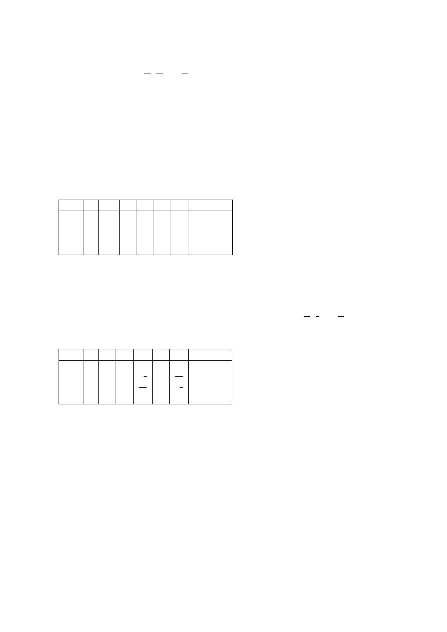
In our example, the pivot column is the column of x
2
(since
−30 < −10) and the pivot
row is row 3 (since min
{
40
3
,
10
1
} =
10
1
); thus, the pivot element is the 1 which lies at the
intersection of column of x
2
and row 3.
Step 5. Make the appropriate transformations to reduce the pivot column to a unit
vector (that is, a vector with 1 in the place of the pivot element and 0 in the rest).
Usually, first we have to divide the pivot row by the pivot element to obtain 1 in the
place of the pivot element. However, this is not necessary in our case since we already
have 1 in that position.
Then the new version of the pivot row is used to get zeros in the other places of the
pivot column. In our example, we multiply the pivot row by 30 and add it to row 0; then
we multiply the pivot row by
−3 and add it to row 1.
Hence we obtain a new simplex tableau:
Row
π
x
1
x
2
d
1
d
2
d
3
Constant
0
1
-10
0
0
0
30
300
1
0
5
0
1
0
-3
10
2
0
1
0
0
1
0
5
3
0
0
1
0
0
1
10
Step 6. Check that row 0 still contains negative values (positive values for a mini-
mization problem). If it does, proceed to step 4. If it does not, the optimal solution must
be found.
In our example, we still have a negative value in row 0 (-10). According to step 4,the
column of x
1
is the pivot column (x
1
enters the base). Since min
{
10
5
,
5
1
} =
10
5
, it follows
that row 1 is the pivot row. Thus, 5 in row 1 is the new pivot element. Applying step 5,
we obtain a third simplex tableau:
Row
π
x
1
x
2
d
1
d
2
d
3
Constant
0
1
0
0
2
0
24
320
1
0
1
0
1
5
0
−3
5
2
2
0
0
0
−1
5
1
3
5
3
3
0
0
1
0
0
1
10
There is no negative element left in row 0 and the current basis consists of x
1
, x
2
, d
2
.
Thus, the optimal solution can be read from the rightmost column: x
1
= 2, x
2
= 10,
d
2
= 3, π = 320. The correspondence between the optimal values and the variables in the
current basis is made using the 1’s in the column vectors of x
1
, x
2
, d
2
.
Example 77 Consider the minimization problem:
Min C = x
1
+ x
2
subject to x
1
− x
2
≥ 0
−x
1
− x
2
≥ −6
x
2
≥ 1
x
1
≥ 0, x
2
≥ 0.
57

After applying step 1 of the simplex algorithm, we obtain:
Min C = x
1
+ x
2
subject to x
1
− x
2
− d
1
= 0
−x
1
− x
2
− d
2
=
−6
x
2
− d
3
= 1
x
1
≥ 0, x
2
≥ 0, d
1
≥ 0, d
2
≥ 0, d
3
≥ 0.
In this example, (0, 0) is not in the feasible set. One way of finding a starting BFS
is to transform the problem by adding 3 more artificial variables f
1
, f
2
, f
3
to the linear
program as follows:
Min C = x
1
+ x
2
+ M (f
1
+ f
2
+ f
3
)
subject to x
1
− x
2
− d
1
+ f
1
= 0
x
1
+ x
2
+ d
2
+ f
2
= 6
x
2
− d
3
+ f
3
= 1
x
1
≥ 0, x
2
≥ 0, d
1
≥ 0, d
2
≥ 0, d
3
≥ 0
f
1
≥ 0, f
2
≥ 0, f
3
≥ 0.
Before adding the artificial variables, the second constraint is multiplied by -1 to obtain a
positive number on the right-hand side.
As long as M is high enough, the optimal solution will contain f
1
= 0, f
2
= 0, f
3
= 0
and thus the optimum is not affected by including the artificial variables in the linear
program. In our case, we choose M = 100. (In maximization problems M is chosen very
low.)
Now, the starting BFS is (x
1
, x
2
, d
1
, d
2
, d
3
, f
1
, f
2
, f
3
) = (0, 0, 0, 0, 0, 0, 6, 1) and the first
simplex tableau is:
Row
C
x
1
x
2
d
1
d
2
d
3
f
1
f
2
f
3
Constant
0
1
-1
-1
0
0
0
-100
-100
-100
0
1
0
1
-1
-1
0
0
1
0
0
0
2
0
1
1
0
1
0
0
1
1
6
3
0
0
1
0
0
-1
0
0
0
1
In order to obtain unit vectors in the columns of f
1
, f
2
and f
3
, we add 100(row1+row2+row3)
to row0:
Row
C
x
1
x
2
d
1
d
2
d
3
f
1
f
2
f
3
Constant
0
1
199
99
-100
100
-100
0
0
0
700
1
0
1
-1
-1
0
0
1
0
0
0
2
0
1
1
0
1
0
0
1
1
6
3
0
0
1
0
0
-1
0
0
0
1
Proceeding with the other steps of the simplex algorithm will finally lead to the optimal
solution x
1
= 1, x
2
= 1, C = 2.
Sometimes the starting BFS (or the starting base) can be found in a simpler way than
by using the general method that was just illustrated. For example, our linear program
58

can be written as:
Min C = x
1
+ x
2
subject to
−x
1
+ x
2
+ d
1
= 0
x
1
+ x
2
+ d
2
= 6
x
2
− d
3
= 1
x
1
≥ 0, x
2
≥ 0, d
1
≥ 0, d
2
≥ 0, d
3
≥ 0.
Taking x
1
= 0, x
2
= 0 we get d
1
= 0, d
2
= 6, d
3
=
−1. Only d
3
contradicts the
constraint d
3
≥ 0. Thus, we need to add only one artificial variable f to the linear
program and the variables in the starting base will be d
1
, d
2
, f .
The complete sequence of simplex tableaux leading to the optimal solution is given
below.
Row
C
x
1
x
2
d
1
d
2
d
3
f
Constant
0
1
-1
-1
0
0
0
-100
0
1
0
-1
1
1
0
0
0
0
2
0
1
1
0
1
0
0
6
3
0
0
1
0
0
-1
1
1
0
1
-1
99
0
0
-100
0
100
1
0
-1
1
∗
1
0
0
0
0
2
0
1
1
0
1
0
0
6
3
0
0
1
0
0
-1
1
1
0
1
98
0
-99
0
-100
0
100
1
0
-1
1
1
0
0
0
0
2
0
2
0
-1
1
0
0
6
3
0
1
∗
0
-1
0
-1
1
1
0
1
0
0
-1
0
-2
-98
2
1
0
0
1
0
0
-1
1
1
2
0
0
0
1
1
2
-2
4
3
0
1
0
-1
0
-1
1
1
(The asterisks mark the pivot elements.)
As can be seen from the last tableau, the optimum is x
1
= 1, x
2
= 1, d
2
= 4, C = 2.
Economics Application 9 (Economic Interpretation of a Maximization Program)
The maximization program in the general form is the production problem facing a firm
which has to produce n goods such that it maximizes its revenue subject to m resource
(factor) constraints.
The variables have the following economic interpretations:
• x
j
is the amount produced of the jth product;
• r
i
is the amount of the ith resource available;
• a
ij
is the amount of the ith resource used in producing a unit of the jth product;
• c
j
is the price of a unit of product j.
The optimal solution to the maximization program indicates the optimal quantities of
each good the firm should produce.
59

Example 78 Let us find an economic interpretation of the maximization program given
in Example 74:
Max π = 10x
1
+ 30x
2
subject to 5x
1
+ 3x
2
≤ 40
x
1
≤ 5
x
2
≤ 10
x
1
≥ 0, x
2
≥ 0.
A firm has to produce two goods using three kinds of resources available in the amounts
40,5,10 respectively. The first resource is used in the production of both goods: five units
are necessary to produce one unit of good 1, and three units to produce 1 unit of good 2.
The second resource is used only in producing good 1 and the third resource is used only
in producing good 2.
The question is, how much of each good should the firm produce in order to maximize
its revenue if the sale prices of goods are 10 and 30, respectively? The solution (2, 10)
gives the optimal amounts the firm should produce.
Economics Application 10 (Economic Interpretation of a Minimization Program)
The minimization program (see the general form) is also connected to the firm’s pro-
duction problem. This time the firm wants to produce a fixed combination of m goods
using n resources (factors). The problem lies in choosing the amount of each resource
such that the total cost of all resources used in the production of the fixed combination of
goods is minimized.
The variables have the following economic interpretations:
• x
j
is the amount of the jth resource used in the production process;
• r
i
is the amount of the good i the firm decides to produce;
• a
ij
is the marginal productivity of resource j in producing good i;
• c
j
is the price of a unit of resource j.
The optimal solution to the minimization program indicates the optimal quantities of
each factor the firm should employ.
Example 79 Consider again the minimization program in example 77:
Min C = x
1
+ x
2
subject to x
1
− x
2
≥ 0
x
1
+ x
2
≤ 6
x
2
≥ 1
x
1
≥ 0, x
2
≥ 0.
What economic interpretation can be assigned to this linear program?
A firm has to produce two goods, at most six units of the first good and one unit of
the second good. Two factors are used in the production process and the price of both
factors is one. The marginal productivity of both factors in producing good 1 is one and
the marginal productivity of the factors in producing good 2 are zero and one, respectively
(good 2 uses only the second factor). The production process also requires that the amount
of the second factor not exceed the amount of the first factor.
The question is how much of each factor the firm should employ in order to minimize
the total factor cost. The solution (1, 1) gives the optimal factor amounts.
60

3.3.3
Duality
As a matter of fact, the maximization and the minimization programs are closely related.
This relationship is called duality.
Definition 48 The dual (program) of the maximization program
Maximize π = c
0
x
subject to Ax
≤ r
and x
≥ 0.
is the minimization program
Minimize π
∗
= r
0
y
subject to A
0
y
≥ c
and y
≥ 0.
Definition 49 The dual (program) of the minimization program
Minimize C = c
0
x
subject to Ax
≥ r
and x
≥ 0.
is the maximization program
Maximize C
∗
= r
0
y
subject to A
0
y
≤ c
and y
≥ 0.
Definition 50 The original program from which the dual is derived is called the primal
(program).
Example 80 The dual of the maximization program in Example 74 is
Min C
∗
= 40y
1
+ 5y
2
+ 10y
3
subject to 5y
1
+ y
2
≥ 10
3y
1
+ y
3
≥ 30
y
1
≥ 0, y
2
≥ 0, y
3
≥ 0.
Example 81 The dual of the minimization program in Example 77 is
Max π
∗
=
−6y
2
+ y
3
subject to y
1
− y
2
≤ 1
−y
1
− y
2
+ y
3
≤ 1
y
1
≥ 0, y
2
≥ 0, y
3
≥ 0.
The following duality theorems clarify the relationship between the dual and the pri-
mal.
Proposition 34 The optimal values of the primal and the dual objective functions are
always identical, if the optimal solutions exist.
61

Proposition 35
1. If a certain choice variable in a primal (dual) program is optimally nonzero then the
corresponding dummy variable in the dual (primal) must be optimally zero.
2. If a certain dummy variable in a primal (dual) program is optimally nonzero then
the corresponding choice variable in the dual (primal) must be optimally zero.
The last simplex tableau of a linear program offers not only the optimal solution to
that program but also the optimal solution to the dual program.
4
!
Recipe 14 – How to solve the dual program:
The optimal solution to the dual program can be read from row 0 of the last simplex
tableau of the primal in the following way:
1. the absolute values of the elements in the columns corresponding to the primal
dummy variables are the values of the dual choice variables.
2. the absolute values of the elements in the columns corresponding to the primal choice
variables are the values of the dual dummy variables.
Example 82 From the last simplex tableau in Example 74 we can infer the optimal so-
lution to the problem in Example 80. It is y
1
= 2, y
2
= 0, y
3
= 24, π
∗
= 320.
Example 83 The last simplex tableau in Example 77 implies that the optimal solution to
the problem in Example 81 is y
1
= 1, y
2
= 0, y
3
= 2, C = 2.
Further reading:
• Intriligator, M. Mathematical Optimization and Economic Theory.
• Luenberger, D.G. Introduction to Linear and Nonlinear Programming.
62

4
Dynamics
4.1
Differential Equations
Definition 51 An equation F (x, y, y
0
, . . . , y
(n)
) = 0 which assumes a functional rela-
tionship between independent variable x and dependent variable y and includes x, y and
derivatives of y with respect to x is called an ordinary differential equation of order n.
The order of a differential equation is determined by the order of the highest derivative
in the equation.
A function y = y(x) is said to be a solution of this differential equation, in some open
interval I, if F (x, y(x), y
0
(x), . . . , y
(n)
(x)) = 0 for all x
∈ I.
4.1.1
Differential Equations of the First Order
Let us consider the first order differential equations, y
0
= f (x, y).
The solution y(x) is said to solve Cauchy’s problem (or the initial value problem) with
the initial values (x
0
, y
0
), if y(x
0
) = y
0
.
Proposition 36 (The Existence Theorem)
If f is continuous in an open domain D, then for any given pair (x
0
, y
0
)
∈ D there
exists a solution y(x) of y
0
= f (x, y) such that y(x
0
) = y
0
.
Proposition 37 (The Uniqueness Theorem)
If f and
∂f
∂y
are continuous in an open domain D, then given any (x
0
, y
0
)
∈ D there
exists a unique solution y(x) of y
0
= f (x, y) such that y(x
0
) = y
0
.
Definition 52 A differential equation of the form y
0
= f (y) is said to be autonomous
(i.e. y
0
is determined by y alone).
Note that the differential equation gives us the slope of the solution curves at all points
of the region D. Thus, in particular, the solution curves cross the curve f (x, y) = k (k is
a constant) with slope k. This curve is called the isocline of slope k. If we draw the set
of isoclines obtained by taking different real values of k, we can schematically sketch the
family of solution curves in the (x
− y)-plane.
Recipe 15 – How to Solve a Differential Equation of the First Order:
There is no general method of solving differential equations. However, in some cases
the solution can be easily obtained:
• The Variables Separable Case.
If y
0
= f (x)g(y) then
dy
g(y)
= f (x)dx. By integrating both parts of the latter equation,
we will get a solution.
Example 84 Solve Cauchy’s problem (x
2
+ 1)y
0
+ 2xy
2
= 0, given y(0) = 1.
If we rearrange the terms, this equation becomes equivalent to
dy
y
2
=
−
2xdx
x
2
+ 1
.
63

The integration of both parts yields
1
y
= ln(x
2
+ 1) + C,
or
y(x) =
1
ln(x
2
+ 1) + C
.
Since we should satisfy the condition y(0) = 1, we can evaluate the constant C,
C = 1.
• Differential Equations with Homogeneous Coefficients.
Definition 53 A function f (x, y) is called homogeneous of degree n, if for any λ
f (λx, λy) = λ
n
f (x, y).
If we have the differential equation M (x, y)dx + N (x, y)dy = 0 and M (x, y), N (x, y)
are homogeneous of the same degree, then the change of variable y = tx reduces this
equation to the variables separable case.
Example 85 Solve (y
2
− 2xy)dx + x
2
dy = 0.
The coefficients are homogeneous of degree 2. Note that y
≡ 0 is a special solution.
If y
6= 0, let us change the variable: y = tx, dy = tdx + xdt. Thus
x
2
(t
2
− 2t)dx + x
2
(tdx + xdt) = 0.
Dividing by x
2
(since y
6= 0, x 6= 0 as well) and rearranging the terms, we get a
variables separable equation
dx
x
=
−
dt
t
2
− t
.
Taking the integrals of both parts,
Z
dx
x
= ln
|x|,
Z
−
dt
t
2
− t
=
Z
1
t
−
1
t
− 1
dt = ln
|t| − ln |t − 1| + C,
therefore
x =
Ct
t
− 1
, or, in terms of y, x =
Cy
y
− x
.
We can single out y as a function of x, y =
x
2
x
− C
.
64

• Exact differential equations.
If we have the differential equation M (x, y)dx + N (x, y)dy = 0 and
∂M (x,y)
∂y
≡
∂N (x,y)
∂x
then all the solutions of this equation are given by F (x, y) = C, C is a constant,
where F (x, y) is such that
∂F
∂x
= M (x, y),
∂F
∂y
= N (x, y).
Example 86 Solve
y
x
dx + (y
3
+ ln x)dy = 0.
∂
∂y
y
x
=
∂
∂x
(y
3
+ ln x), so we have checked that we are dealing with an exact
differential equation. Therefore, we need to find F (x, y) such that
F
0
x
=
y
x
=
⇒ F (x, y) =
Z
y
x
dx = y ln x + φ(y),
and
F
0
y
= y
3
+ ln x.
To find φ(y), note that
F
0
y
= y
3
+ ln x = ln x + φ
0
(y) =
⇒ φ(y) =
Z
y
3
dy =
1
4
y
4
+ C.
Therefore, all solutions are given by the implicit function 4y ln x + y
4
= C.
• Linear differential equations of the first order.
If we need to solve y
0
+ p(x)y = q(x), then all the solutions are given by the formula
y(x) = e
−
R
p(x)dx
C +
Z
q(x)e
R
p(x)dx
dx
.
Example 87 Solve xy
0
− 2y = 2x
4
.
In other words, we need to solve y
0
−
2
x
y = 2x
3
. Therefore,
y(x) = e
R
2
x
dx
C +
Z
2x
3
e
−
R
2
x
dx
sd
= e
ln x
2
C +
Z
2x
3
e
ln
1
x2
sd
= x
2
(C + x
2
).
4.1.2
Linear Differential Equations of a Higher Order with Constant Coeffi-
cients
These are the equations of the form
y
(n)
+ a
1
y
(n
−1)
+ . . . + a
n
−1
y
0
+ a
n
y = f (x).
If f (x)
≡ 0 the equation is called homogeneous, otherwise it is called non-homogeneous.
65

Recipe 16 How to find the general solution y
g
(x) of the homogeneous equation: The general
solution is a sum of basic solutions y
1
, . . . , y
n
,
y
g
(x) = C
1
y
1
(x) + . . . + C
n
y
n
(x),
C
1
, . . . , C
n
are arbitrary constants.
These arbitrary constants, however, can be defined in a unique way, once we set up the
initial value Cauchy problem. Find y(x) such that
y(x) = y
0
0
, y
0
(x) = y
0
1
, . . . , y
(n
−1)
(x) = y
0
n
−1
at x = x
0
,
where x
0
, y
0
0
, y
0
1
, . . . , y
0
n
−1
are given initial values (real numbers).
To find all basic solutions, we proceed as follows:
1. Solve the characteristic equation
λ
n
+ a
1
λ
n
−1
+ . . . + a
n
−1
λ + a
n
= 0
for λ. The roots of this equation are λ
1
, . . . , λ
n
. Some of these roots may be complex
numbers. We may also have repeated roots.
2. If λ
i
is a simple real root, the basic solution corresponding to this root is y
i
(x) = e
λ
i
x
.
3. If λ
i
is a repeated real root of degree k, it generates k basic solutions
y
i
1
(x) = e
λ
i
x
, y
i
2
(x) = xe
λ
i
x
, . . . , y
i
k
(x) = x
k
−1
e
λ
i
x
.
4. If λ
j
is a simple complex root, λ
j
= α
j
+ iβ
j
, i =
√
−1, then the complex conjugate
of λ
j
, say λ
j+1
= α
j
− iβ
j
, is also a root of the characteristic equations. Therefore
the pair λ
j
, λ
j+1
give rise to two basic solutions:
y
j
1
= e
α
j
x
cos β
j
x,
y
j
2
= e
α
j
x
sin β
j
x.
5. If λ
j
is a repeated complex root of degree l, λ
j
= α
j
+ iβ
j
, then the complex conjugate
of λ
j
, say λ
j+1
= α
j
−iβ
j
, is also a repeated root of degree l. These 2l roots generate
2l basic solutions
y
j
1
= e
α
j
x
cos β
j
x, y
j
2
= xe
α
j
x
cos β
j
x, . . . , y
j
l
= x
l
−1
e
α
j
x
cos β
j
x,
y
j
l+1
= e
α
j
x
sin β
j
x, y
j
l+2
= xe
α
j
x
sin β
j
x, . . . , y
j
2l
= x
l
−1
e
α
j
x
sin β
j
x.
Recipe 17 – How to Solve the Non-Homogeneous Equation:
The general solution of the nonhomogeneous solution is y
nh
(x) = y
g
(x) + y
p
(x), where
y
g
(x) is the general solution of the homogeneous equation and y
p
(x) is a particular solution
of the nonhomogeneous equation, i.e. any function which solves the nonhomogeneous
equation.
Recipe 18 – How to Find a Particular Solution of the Non-Homogeneous Equation:
66

1. If f (x) = P
k
(x)e
bx
, P
k
(x) is a polynomial of degree k, then a particular solution is
y
p
(x) = x
s
Q
k
(x)e
bx
,
where Q
k
(x) is a polynomial of the same degree k. If b is not a root of the charac-
teristic equation, s = 0; if b is a root of the characteristic polynomial of degree m
then s = m.
2. If f (x) = P
k
(x)e
px
cos qx + Q
k
(x)e
px
sin qx, P
k
(x), Q
k
(x) are polynomials of degree
k, then a particular solution can be found in the form
y
p
(x) = x
s
R
k
(x)e
px
cos qx + x
s
T
k
(x)e
px
sin qx,
where R
k
(x), T
k
(x) are polynomials of degree k. If p + iq is not a root of the charac-
teristic equation, s = 0; if p + iq is a root of the characteristic polynomial of degree
m then s = m.
3. The general method for finding a particular solution of a nonhomogeneous equation
is called the variation of parameters or the method of undetermined coefficients.
Suppose we have the general solution of the homogeneous equation
y
g
= C
1
y
1
(x) + . . . + C
n
y
n
(x),
where y
i
(x) are basic solutions. Treating constants C
1
, . . . , C
n
as functions of x, for
instance, u
1
(x), . . . , u
n
(x), we can express a particular solution of the nonhomoge-
neous equation as
y
p
(x) = u
1
(x)y
1
(x) + . . . + u
n
(x)y
n
(x),
where u
1
(x). . . . , u
n
(x) are solutions of the system
u
0
1
(x)y
1
(x) + . . . + u
0
n
(x)y
n
(x) = 0,
u
0
1
(x)y
0
1
(x) + . . . + u
0
n
(x)y
0
n
(x) = 0,
. . . . . . . . .
u
0
1
(x)y
(n
−2)
1
(x) + . . . + u
0
n
(x)y
(n
−2)
n
(x) = 0,
u
0
1
(x)y
(n
−1)
1
(x) + . . . + u
0
n
(x)y
(n
−1)
n
(x) = f (x)
4. If f (x) = f
1
(x) + f
2
(x) + . . . + f
r
(x) and y
p1
(x), . . . , y
pr
(x) are particular solutions
corresponding to f
1
(x), . . . , f
r
(x) respectively, then
y
p
(x) = y
p1
(x) + . . . + y
pr
(x).
67

Example 88 Solve y
00
− 5y
0
+ 6y = x
2
+ e
x
− 5.
The characteristic roots are λ
1
= 2, λ
2
= 3, therefore the general solution of the
homogeneous equation is
y(t) = C
1
e
2t
+ C
2
e
3t
.
We search for a particular solution in the form
y
p
(t) = at
2
+ bt + c + de
t
.
To find coefficients a, b, c, d, let us substitute the particular solution into the initial
equation:
2a + de
t
− 5(2at + b + de
t
) + 6(at
2
+ bt + c + de
t
) = t
2
− 5 + e
t
.
Equating term-by-term the coefficients at the left-hand side to the right-hand side, we
obtain
6a = 1,
−5 · 2a + 6 · b = 0,
2a
− 5b + 6c = −5,
d
− 5d + 6d = 1.
Thus d = 1/2, a = 1/6,
b = 10/36,
c =
−71/108.
Finally, the general solution of the nonhomogeneous equation is
y
nh
(x) = y(t) = C
1
e
2t
+ C
2
e
3t
+
x
2
6
+
5x
18
−
71
108
+
e
x
2
.
Example 89 Solve y
00
− 2y
0
+ y =
e
x
x
.
The general solution of the homogeneous equation is y
g
(x) = C
1
xe
x
+ C
2
e
x
(the char-
acteristic equation has the repeated root λ = 1 of degree 2). We look for a particular
solution of the nonhomogeneous equation in the form
y
p
(x) = u
1
(x)xe
x
+ u
2
(x)e
x
.
We have
u
0
1
(x)xe
x
+ u
0
2
(x)e
x
= 0,
u
0
1
(x)(e
x
+ xe
x
) + u
0
2
(x)e
x
=
e
x
x
.
Therefore u
0
1
(x) =
1
x
, u
0
2
(x) =
−1. Integrating, we find that u
1
(x) = ln
|x|, u
2
(x) =
−x.
Thus y
p
(x) = ln
|x|xe
x
+ xe
x
, and
y
n
(x) = y
g
(x) + y
p
(x) = ln
|x|xe
x
+ C
1
xe
x
+ C
2
e
x
.
4.1.3
Systems of the First Order Linear Differential Equations
The general form of a system of the first order differential equations is:
˙x(t) = A(t)x(t) + b(t),
x(0) = x
0
where t is the independent variable (“time”), x(t) = (x
1
(t), . . . , x
n
(t))
0
is a vector of
dependent variables, A(t) = (a
ij
(t))
[n
×n]
is a real n
× n matrix with variable coefficients,
b(t) = (b
1
(t), . . . , b
n
(t))
0
a variant n-vector.
68

In what follows, we concentrate on the case when A and b do not depend on t, which
is the case in constant coefficients differential equations systems:
˙x(t) = Ax(t) + b,
x(0) = x
0
.
(11)
We also assume that A is non-singular.
The solution of system (11) can be determined in two steps:
• First, we consider the homogeneous system (corresponding to b = 0):
˙x(t) = Ax(t),
x(0) = x
0
(12)
The solution x
c
(t) of this system is called the complementary solution.
• Second, we find a particular solution x
p
of the system (11), which is called the
particular integral. The constant vector x
p
is simply the solution to Ax
p
=
−b, i.e.
x
p
=
−A
−1
b.
5
Given x
c
(t) and x
p
, the general solution of the system (11) is simply:
x(t) = x
c
(t) + x
p
We can find the solution to the homogeneous system (12) in two different ways.
First, we can eliminate n
−1 unknowns and reduce the system to one linear differential
equation of degree n.
Example 90 Let
(
˙x = 2x + y,
˙
y = 3x + 4y.
Taking the derivative of the first equation and eliminating y and ˙
y ( ˙
y = 3x + 4y =
3x + 4 ˙x
− 4 · 2x), we arrive at the second order homogeneous linear differential equation
¨
x
− 6 ˙x + 5x = 0,
which has the general solution x(t) = C
1
e
t
+ C
2
e
5t
. Since y(t) = ˙x
− 2x, we find that
y(t) =
−C
1
e
t
+ 3C
2
e
5t
.
The second way is to write the solution to (12) as
x(t) = e
At
x
0
where (by definition)
e
At
= I + At +
A
2
t
2
2!
+
· · ·
5
In a sense, x
p
can be viewed as an affine shift, which restores the origin to a unique equilibrium of
(11).
69

Unfortunately, this formula is of little practical use. In order to find a feasible formula
for e
At
, we distinguish three main cases.
Case 1: A has real and distinct eigenvalues
The fact that the eigenvalues are real and distinct implies that any corresponding
eigenvectors are linearly independent. Consequently, A is diagonalizable, i.e.
A = P ΛP
−1
where P = [v
1
, v
2
, . . . , v
n
] is a matrix composed by the eigenvectors of A and Λ is a
diagonal matrix whose diagonal elements are the eigenvalues of A.
Therefore, e
A
=
P e
Λ
P
−1
.
Thus, the solution of the system (12) can be written as:
x(t) = P e
Λt
P
−1
x
0
= P e
Λt
c
= c
1
v
1
e
λ
1
t
+ . . . + c
n
v
n
e
λ
n
t
where c = (c
1
, c
2
, . . . , c
n
) is a vector of constants determined from the initial conditions
(c = P
−1
x
0
).
Case 2: A has real and repeated eigenvalues
First, consider the simpler case when A has only one eigenvalue λ which is repeated
m times (m is called the algebraic multiplicity of λ). Generally, in this situation the
maximum number of independent eigenvectors corresponding to λ is less than m, meaning
that we cannot construct the matrix P of linearly independent eigenvectors and, therefore,
A is not diagonalizable.
6
The solution in this case has the form:
x(t) =
m
X
i=1
c
i
h
i
(t)
where h
i
(t) are quasipolinomials and c
i
are constants determined by the initial conditions.
For example, if m = 3, we have:
h
1
(t) = e
λt
v
1
h
2
(t) = e
λt
(tv
1
+ v
2
)
h
3
(t) = e
λt
(t
2
v
1
+ 2tv
2
+ 3v
3
)
where v
1
, v
2
, v
3
are determined by the conditions:
(A
− λI)v
i
= v
i
−1
, v
0
= 0;
If A happens to have several eigenvalues which are repeated, the solution of (12) is
obtained by finding the solution corresponding to each eigenvalue, and then adding up
the individual solutions.
6
If A is a real and symmetric matrix, then A is always diagonalizable and the formula given for case
1 can be applied.
70

Case 3: A has complex eigenvalues.
Since A is a real matrix, the complex eigenvalues always appear in pairs, i.e. if A has
the eigenvalue α + βi, then it also must have the eigenvalue α
− βi.
Now consider the simpler case when A has only one pair of complex eigenvalues,
λ
1
= α + βi and λ
2
= α
− βi. Let v
1
and v
2
denote the eigenvectors corresponding to λ
1
and λ
2
; then v
2
= ¯
v
1
, where ¯
v
1
is the conjugate of v
1
. The solution can be expressed as:
x(t) = e
At
x
0
= P e
Λt
P
−1
x
0
= P e
Λt
c
= c
1
v
1
e
(α+βi)t
+ c
2
v
2
e
(α
−βi)t
= c
1
v
1
e
αt
(cos βt + i sin βt) + c
2
v
2
e
αt
(cos βt
− i sin βt)
= (c
1
v
1
+ c
2
v
2
)e
αt
cos βt + i(c
1
v
1
− c
2
v
2
)e
αt
sin βt
= h
1
e
αt
cos βt + h
2
e
αt
sin βt,
where h
1
= c
1
v
1
+ c
2
v
2
, h
2
= i(c
1
v
1
− c
2
v
2
) are real vectors.
Note that if A has more pairs of complex eigenvalues, then the solution of (12) is
obtained by finding the solution corresponding to each eigenvalue, and then adding up
the individual solutions. The same remark holds true when we encounter any combination
of the three cases discussed above.
Example 91 Consider
A =
5
2
−4 −1
!
.
Solving the characteristic equation det(A
− λI) = λ
2
− 4λ + 3 = 0 we find eigenvalues
of A: λ
1
= 1, λ
2
= 3.
From the condition (A
− λ
1
I)v
1
= 0 we find an eigenvector corresponding to λ
1
:
v
1
=
−1
2
!
.
Similarly, the condition (A
− λ
2
I)v
2
= 0 gives an eigenvector corresponding to λ
2
:
v
2
=
−1
1
!
.
Therefore, the general solution of the system ˙x(t) = Ax(t) is
x(t) = c
1
v
1
e
λ
1
t
+ c
2
v
2
e
λ
2
t
or
x(t) =
x
1
(t)
x
2
(t)
!
=
−c
1
e
t
− c
2
e
3t
2c
1
e
t
+ c
2
e
3t
!
.
Example 92 Consider
A =
3
1
−1 1
!
.
71

det(A
− λI) = λ
2
− 4λ + 4 = 0 gives the eigenvalue λ = 2 repeated twice.
From the condition (A
− λ
1
I)v
1
= 0 we find v
1
=
−1
1
!
and from (A
− λ
1
I)v
2
= v
1
we obtain v
2
=
1
−2
!
.
The solution of the system ˙x(t) = Ax(t) is
x(t) = c
1
h
1
(t) + c
2
h
2
(t)
= c
1
v
1
e
λt
+ c
2
(tv
1
+ v
2
)e
λt
or
x(t) =
x
1
(t)
x
2
(t)
!
=
−c
1
+ c
2
− c
2
t
c
1
− 2c
2
+ c
2
t
!
e
2t
.
Example 93 Consider
A =
3
2
−1 1
!
.
The equation det(A
−λI) = λ
2
−4λ+5 = 0 leads to the complex eigenvalues λ
1
= 2+i,
λ
2
= 2
− i.
For λ
1
we set the equation (A
− λ
1
I)v
1
= 0 and obtain:
v
1
=
1 + i
−1
!
v
2
= ¯
v
1
=
1
− i
−1
!
.
The solution of the system ˙x(t) = Ax(t) is
x(t) = c
1
v
1
e
λ
1
t
+ c
2
v
2
e
λ
2
t
= c
1
v
1
e
(2+i)t
+ c
2
(tv
1
+ v
2
)e
(2
−i)t
= c
1
v
1
e
2t
(cos t + i sin t) + c
2
v
2
e
2t
(cos t
− i sin t).
Performing the computations, we finally obtain:
x(t) = (c
1
+ c
2
)e
2t
cos t
− sin t
− cos t
!
+ i(c
1
− c
2
)e
2t
cos t + sin t
− sin t
!
.
Now let the vector b be different from 0. To specify the solution to the system (11), we
need a particular solution x
p
. This is found from the condition ˙x = 0; thus, x
p
=
−A
−1
b.
Therefore, the general solution of the non-homogeneous system is
x(t) = x
c
(t) + x
p
= P e
Λt
P
−1
c
− A
−1
b
where the vector of constants c is determined by the initial condition x(0) = x
0
as c =
x
0
+ A
−1
b.
72

Example 94 Consider
A =
5
2
−4 −1
!
, b =
1
2
!
and x
0
=
−1
2
!
.
In Example 91 we obtained
x
c
(t) =
−c
1
e
t
− c
2
e
3t
2c
1
e
t
+ c
2
e
3t
!
.
In addition, we have
c =
c
1
c
2
!
= x
0
+ A
−1
b =
−1
2
!
+
−5
3
14
3
!
=
−8
3
20
3
!
and
−x
p
= A
−1
b =
−1
3
−2
3
4
3
5
3
!
1
2
!
=
−5
3
14
3
!
.
The solution of the system ˙x(t) = Ax(t) + b is
x(t) = x
c
(t) + x
p
=
8
3
e
t
−
20
3
e
3t
+
5
3
−16
3
e
t
+
20
3
e
3t
+
−14
3
!
.
Economics Application 11 (General Equilibrium)
Consider a market for n goods x = (x
1
, x
2
, . . . , x
n
)
0
. Let p = (p
1
, p
2
, . . . , p
n
)
0
denote the
vector of prices and D
i
(p), S
i
(p) demand and supply for good i, i = 1, . . . , n. The general
equilibrium is obtained for a price vector p
∗
which satisfies the conditions: D
i
(p
∗
) = S
i
(p
∗
)
for all i = 1, . . . , n.
The dynamics of price adjustment for the general equilibrium can be described by a
system of first order differential equations of the form:
˙
p = W [D(p)
− S(p)] = W Ap,
p(0) = p
0
where W = diag(w
i
) is a diagonal matrix having the speeds of adjustment w
i
, i = 1, . . . , n,
D(p) = [D
1
(p), . . . , D
n
(p)]
0
on the diagonal and S(p) = [S
1
(p), . . . , S
n
(p)]
0
are linear func-
tions of p and A is a constant n
× n matrix.
We can solve this system by applying the methods discussed above. For instance, if
W A = P ΛP
−1
, then the solution is
p(t) = P e
Λt
P
−1
p
0
.
Economics Application 12 (The Dynamic IS-LM Model)
A simplified dynamic IS-LM model can be specified by the following system of differ-
ential equations:
˙
Y
= w
1
(I
− S)
˙r = w
2
[L(Y, r)
− M],
with initial conditions
Y (0) = Y
0
, r(0) = r
0
,
where:
73

• Y is national income;
• r is the interest rate;
• I = I
0
− αr is the investment function (α is a positive constant);
• S = s(Y −T )+(T −G) is national savings; (T, G and s represents taxes, government
purchases and the savings rate);
• L(Y, r) = a
1
Y
− a
2
r is money demand (a
1
and a
2
are positive constants);
• M is money supply;
• w
1
, w
2
are speeds of adjustment.
For simplicity, consider w
1
= 1 and w
2
= 1. The original system can be re-written as:
˙
Y
˙r
!
=
−s −α
a
1
−a
2
!
Y
r
!
+
I
0
− (1 − s)T + G
−M
!
Assume that A =
−s −α
a
1
−a
2
!
is diagonalizable, i.e. A = P ΛP
−1
, and has distinct
eigenvalues λ
1
, λ
2
with corresponding eigenvectors v
1
, v
2
. (λ
1
, λ
2
are the solutions of the
equation r
2
+ (s + a
2
)r + sa
2
+ αa
1
= 0.)
The solution becomes:
Y (t)
r(t)
!
= P e
Λt
P
−1
(x
0
+ A
−1
b)
− A
−1
b
where
x
0
=
Y
0
r
0
!
, b =
I
0
− (1 − s)T + G
−M
#
.
We have
A
−1
=
1
αa
1
+ sa
2
−a
2
α
−a
1
−s
!
and
A
−1
b =
1
αa
1
+ sa
2
−a
2
[I
0
− (1 − s)T + G] − αM
−a
1
[I
0
− (1 − s)T + G] + sM
!
Assume that P
−1
=
˜
v
1
0
˜
v
2
0
!
. Then, we have:
P e
Λt
P
−1
= [v
1
, v
2
]
e
λ
1
t
0
0
e
λ
2
t
!
˜
v
1
0
˜
v
2
0
!
= v
1
˜
v
1
0
e
λ
1
t
+ v
2
˜
v
2
0
e
λ
2
t
.
Finally, the solution is:
Y (t)
r(t)
!
= [v
1
˜
v
1
0
e
λ
1
t
+ v
2
˜
v
2
0
e
λ
2
t
]
Y
0
+
−a
2
S
−αM
αa
1
+sa
2
r
0
+
−a
1
S+sM
αa
1
+sa
2
!
−
−a
2
S
−αM
αa
1
+sa
2
−a
1
S+sM
αa
1
+sa
2
!
,
where S = I
0
− (1 − s)T + G.
74

Economics Application 13 (The Solow Model)
The Solow model is the basic model of economic growth and it relies on the following
key differential equation, which explains the dynamics of capital per unit of effective labor:
˙k(t) = sf(k(t)) − (n + g + δ)k(t),
k(0) = k
0
where
• k denotes capital per effective labor;
• s is the savings rate;
• n is the rate of population growth;
• g is the rate of technological progress;
• δ is the depreciation rate.
Let us consider two types of production function.
Case 1. The production function is linear: f (k(t)) = ak(t) where a is a positive
constant.
The equation for ˙k becomes:
˙k(t) = (sa − n − g − δ)k(t).
This linear differential equation has the solution
k(t) = k(0)e
(sa
−n−g−δ)t
= k
0
e
(sa
−n−g−δ)t
.
Case 2. The production function takes the Cobb-Douglas form: f (k(t)) = [k(t)]
α
where α
∈ [0, 1].
In this case, the equation for ˙k represents a Bernoulli nonlinear differential equation:
˙k(t) + (n + g + δ)k(t) = s[k(t)]
α
,
k(0) = k
0
Dividing both sides of the latter equation by [k(t)]
α
, and denoting m(t) = [k(t)]
1
−α
, m(0) =
(k
0
)
1
−α
, we obtain:
1
1
− α
˙
m(t) + (n + g + δ)m(t) = s,
or
˙
m(t) + (1
− α)(n + g + δ)m(t) = s(1 − α).
The solution to this first order linear differential equation is given by:
m(t) = e
−
R
(1
−α)(n+g+δ)dt
[A +
Z
s(1
− α)e
R
(1
−α)(n+g+δ)dt
dt]
= e
−(1−α)(n+g+δ)t
[A + s(1
− α)
Z
e
(1
−α)(n+g+δ)t
dt]
= Ae
−(1−α)(n+g+δ)t
+
s
n + g + δ
.
75

where A is determined from the initial condition m(0) = (k
0
)
1
−α
. It follows that A =
(k
0
)
1
−α
−
s
n+g+δ
and
m(t) = [(k
0
)
1
−α
−
s
n + g + δ
]e
−(1−α)(n+g+δ)t
+
s
n + g + δ
,
k(t) =
{[(k
0
)
1
−α
−
s
n + g + δ
]e
−(1−α)(n+g+δ)t
+
s
n + g + δ
}
1
1
−α
.
Economics Application 14 (The Ramsey-Cass-Koopmans Model)
This model takes capital per effective labor k(t) and consumption per effective labor c(t)
as endogenous variables. Their behavior is described by the following system of differential
equations:
˙k(t) = f(k(t)) − c(t) − (n + g)k(t)
˙c(t) =
f
0
(k(t))
− ρ − θg
θ
c(t)
with the initial conditions
k(0) = k
0
, c(0) = c
0
,
where, in addition to the variables already specified in the previous application,
• ρ stands for the discount rate ;
• θ is the coefficient of relative risk aversion.
Assume again that f (k(t)) = ak(t) where a > 0 is a constant. The initial system
reduces to a system of linear differential equations:
˙k(t) = (a − n − g)k(t) − c(t)
˙c(t) =
a
− ρ − θg
θ
c(t)
The second equation implies that:
c(t) = c
0
e
bt
, where b =
a
− ρ − θg
θ
.
Substituting for c(t) in the first equation, we obtain:
˙k(t) = (a − n − g)k(t) − c
0
e
bt
The solution of this linear differential equation takes the form:
k(t) = k
c
(t) + k
p
(t)
where k
c
and k
p
are the complementary solution and the particular integral, respectively.
The homogeneous equation ˙k(t) = (a
− n − g)k(t) gives the complementary solution:
k(t) = k
0
e
(a
−n−g)t
.
The particular integral should be of the form k
p
(t) = me
bt
; the value of m can be
determined by substituting k
p
in the non-homogeneous equation for ˙k:
mbe
bt
= (a
− n − g)me
bt
− c
0
e
bt
76

It follows that
m =
c
0
a
− n − g − b
,
k
p
(t) =
c
0
a
− n − g − b
e
bt
and
k(t) = k
0
e
(a
−n−g)t
+
c
0
a
− n − g − b
e
bt
.
4.1.4
Simultaneous Differential Equations. Types of Equilibria
Let x = x(t), y = y(t), where t is independent variable. Then consider a two-dimensional
autonomous system of simultaneous differential equations
dx
dt
= f (x, y),
dy
dt
= g(x, y).
The point (x
∗
, y
∗
) is called an equilibrium of this system if f (x
∗
, y
∗
) = g(x
∗
, y
∗
) = 0.
Let
J be the Jacobian matrix
J =
∂f
∂x
∂f
∂y
∂g
∂x
∂g
∂y
!
evaluated at (x
∗
, y
∗
), and let λ
1
, λ
2
be the eigenvalues of this Jacobian.
Then the equilibrium is
1. a stable (unstable) node if λ
1
, λ
2
are real, distinct and both negative (positive);
2. a saddle if the eigenvalues are real and of different signs, i.e. λ
1
λ
2
< 0;
3. a stable (unstable) focus if λ
1
, λ
2
are complex and Re(λ
1
) < 0 (Re(λ
1
) > 0);
4. a center or a focus if λ
1
, λ
2
are complex and Re(λ
1
) = 0;
5. a stable (unstable) improper node if λ
1
, λ
2
are real, λ
1
= λ
2
< 0 (λ
1
= λ
2
> 0) and
the Jacobian is a not diagonal matrix;
6. a stable (unstable) star node if λ
1
, λ
2
are real, λ
1
= λ
2
< 0 (λ
1
= λ
2
> 0) and the
Jacobian is a diagonal matrix.
The figure below illustrates this classification:
77

1) Node
2) Saddle
4) Center
5) Improper node
6) Star node
3) Focus
p
p
p
p
p
Example 95 Find the equilibria of the system and classify them
(
˙x = 2xy
− 4y − 8,
˙
y = 4y
2
− x
2
.
Solving the system
2xy
− 4y − 8 = 0,
4y
2
− x
2
= 0
for x, y, we find two equilibria, (
−2, −1) and (4, 2).
At (
−2, −1) the Jacobian
J =
2y
2x
− 4
−2x
8y
!
(
−2,−1)
=
−2 −8
4
−8
!
.
The characteristic equation for J is λ
2
− (tr(J))λ + det(J) = 0.
(tr(J ))
2
− 4 det(J)) < 0 =⇒ λ
1,2
are complex.
78

tr(J ) < 0 =
⇒ λ
1
+ λ
2
< 0 =
⇒ Reλ
1
< 0 =
⇒ the equilibrium (−2, −1) is a stable
focus.
At (4, 2)
J =
4
4
−8 16
!
.
(tr(J ))
2
− 4 det(J)) > 0 =⇒ λ
1,2
are distinct and real.
tr(J ) = λ
1
+ λ
2
> 0, det(J ) = λ
1
λ
2
> 0 =
⇒ λ
1
> 0, λ
2
> 0 =
⇒ the equilibrium (4, 2)
is an unstable node.
4.2
Difference Equations
Let y denote a real-valued function defined over the set of natural numbers. Hereafter y
k
stands for y(k) – the value of y at k, where k = 0, 1, 2, . . ..
Definition 54
• The first difference of y evaluated at k is ∆y
k
= y
k+1
− y
k
.
• The second difference of y evaluated at k is ∆
2
y
k
= ∆(∆y
k
) = y
k+2
− 2y
k+1
+ y
k
.
• In general, the nth difference of y evaluated at k is defined as ∆
n
y
k
= ∆(∆
n
−1
y
k
),
for any integer n, n > 1.
Definition 55 A difference equation in the unknown y is an equation relating y and any
of its differences ∆y, ∆
2
y, . . . for each value of k, k = 0, 1, . . ..
Solving a difference equation means finding all functions y which satisfy the relation
specified by the equation.
Example 96 (Examples of Difference Equations)
• 2∆y
k
− y
k
= 1 (or, equivalently, 2∆y
− y = 1)
• ∆
2
y
k
+ 5y
k
∆y
k
+ (y
k
)
2
= 2 (or ∆
2
y + 5y∆y + (y)
2
= 2)
Note that any difference equation can be written as
f (y
k+n
, y
k+n
−1
, . . . , y
k+1
, y
k
) = g(k), n
∈ N
For example, the above two equations may also be expressed as follows:
• 2y
k+1
− 3y
k
= 1
• y
k+2
− 2y
k+1
+ y
k
+ 5y
k
y
k+1
− 4(y
k
)
2
= 2
Definition 56 A difference equation is linear if it takes the form
f
0
(k)y
k+n
+ f
1
(k)y
k+n
−1
+ . . . + f
n
−1
(k)y
k+1
+ f
n
(k)y
k
= g(k),
where f
0
, f
1
, . . . , f
n
, g are each functions of k (but not of some y
k+i
, i
∈ N) defined for
all k = 0, 1, 2, . . ..
79

Definition 57 A linear difference equation is of order n if both f
0
(k) and f
n
(k) are
different from zero for each k = 0, 1, 2, . . ..
From now on, we focus on the problem of solving linear difference equations of order
n with constant coefficients. The general form of such an equation is:
f
0
y
k+n
+ f
1
y
k+n
−1
+ . . . + f
n
−1
y
k+1
+ f
n
y
k
= g
k
,
where, this time, f
0
, f
1
, . . . , f
n
are real constants and f
0
, f
n
are different from zero.
Dividing this equation by f
0
and denoting a
i
=
f
i
f
0
for i = 0, . . . , n, r
k
=
g
k
f
0
, the general
form of a linear difference equation of order n with constant coefficients becomes:
y
k+n
+ a
1
y
k+n
−1
+ . . . + a
n
−1
y
k+1
+ a
n
y
k
= r
k
,
(13)
where a
n
is non-zero.
Recipe 19 – How to Solve Difference Equation: General Procedure:
The general procedure for solving a linear difference equation of order n with constant
coefficients involves three steps:
Step 1. Consider the homogeneous equation
y
k+n
+ a
1
y
k+n
−1
+ . . . + a
n
−1
y
k+1
+ a
n
y
k
= 0,
and find its solution Y . (First we will describe and illustrate the solving procedure
for equations of order 1 and 2. Following that, the theory for the case of order n is
obtained as a natural extension of the theory for second-order equations.)
Step 2. Find a particular solution y
∗
of the complete equation (13). The most useful tech-
nique for finding particular solutions is the method of undetermined coefficients
which will be illustrated in the examples that follow.
Step 3. The general solution of equation (13) is:
y
k
= Y + y
∗
.
4.2.1
First-order Linear Difference Equations
The general form of a first-order linear differential equation is:
y
k+1
+ ay
k
= r
k
.
The corresponding homogeneous equation is:
y
k+1
+ ay
k
= 0,
and has the solution Y = C(
−a)
k
, where C is an arbitrary constant.
80

Recipe 20 – How to Solve a First-Order Non-Homogeneous Linear Difference Equation:
First, consider the case when r
k
is constant over time, i.e. r
k
≡ r for all k.
Much as in the case of linear differential equations, the general solution of the non-
homogeneous difference equation y
t
is the sum of the general solution of the homogeneous
equation and a particular solution of the nonhomogeneous equation. Therefore
y
k
= A
· (−a)
k
+
r
1 + a
,
a
6= −1,
y
k
= A
· (−a)
k
+ rk = A + rk,
a =
−1,
where A is an arbitrary constant.
If we have the initial condition y
k
= y
0
when k = 0, the general solution of the
nonhomogeneous equation takes the form
y
k
=
y
0
−
r
1 + a
× (−a)
k
+
r
1 + a
,
a
6= −1,
y
k
= y
0
+ rk,
a =
−1.
If r now depends on k, r = r
k
, then the solution takes the form
y
k
= (
−a)
k
y
0
+
k
−1
X
i=0
(
−a)
k
−1−i
r
i
,
k = 1, 2, . . .
A particular solution to non-homogeneous difference equation can be found using the
method of undetermined coefficients.
Example 97 y
k+1
− 3y
k
= 2.
The solution of the homogeneous equation y
k+1
− 3y
k
= 0 is: Y = C
· 3
k
. The right-
hand term suggests looking for a constant function as a particular solution. Assuming
y
∗
= A and substituting into the initial equation, we obtain A =
−1; hence y
∗
=
−1 and
the general solution is y
k
= Y + y
∗
= C3
k
− 1.
Example 98 y
k+1
− 3y
k
= k
2
+ k + 2.
The homogeneous equation is the same as in the preceding example. But the right-hand
term suggests finding a particular solution of the form:
y
∗
= Ak
2
+ Bk + D.
Substituting y
∗
into non-homogeneous equation, we have:
A(k + 1)
2
+ B(k + 1) + D
− 3Ak
2
− 3Bk − 3D = k
2
+ k + 2, or
−2Ak
2
+ 2(A
− B)k + A + B − 2D = k
2
+ k + 2.
In order to satisfy this equality for each k, we must have:
−2A = 1
2(A
− B) = 1
A + B
− 2D = 2.
It follows that A =
−
1
2
, B =
−1, D = −
3
4
and y
∗
=
−
1
2
k
2
− k −
3
4
. The general solution
is y
k
= Y + y
∗
= C3
k
−
1
2
k
2
− k −
3
4
.
81

Example 99 y
k+1
− 3y
k
= 4e
k
.
This time we try a particular solution of the form: y
∗
= Ae
k
. After substitution, we
find A =
4
e
−3
. The general solution is y
k
= Y + y
∗
= C3
k
+
4e
k
e
−3
.
Two remarks:
• The method of undetermined coefficients illustrated by these examples applies to
the general case of order n as well. The trial solutions corresponding to some simple
functions r
k
are given in the following table:
Right-hand term r
k
Trial solution y
∗
a
k
Aa
k
k
n
A
0
+ A
1
k + A
2
k
2
+ . . . + A
n
k
n
sin ak or cos ak
A sin ak + B cos ak
• If the function r is a combination of simple functions for which we know the trial
solutions, then a trial solution for r can be obtained by combining the trial solutions
for the simple functions. For example, if r
k
= 5
k
k
3
, then the trial solution would be
y
∗
= 5
k
(A
0
+ A
1
k + A
2
k
2
+ A
3
k
3
).
4.2.2
Second-Order Linear Difference Equations
The general form is:
y
k+2
+ a
1
y
k+1
+ a
2
y
k
= r
k
.
(14)
The solution to the corresponding homogeneous equation
y
k+2
+ a
1
y
k+1
+ a
2
y
k
= 0
(15)
depends on the solutions to the quadratic equation:
m
2
+ a
1
m + a
2
= 0,
which is called the auxiliary (or characteristic) equation of equation (14). Let m
1
, m
2
denote the roots of the characteristic equation. Then, both m
1
and m
2
will be non-zero
because a
2
is non-zero for (14) to be of second order.
Case 1. m
1
and m
2
are real and distinct.
The solution to (15) is Y = C
1
m
k
1
+ C
2
m
k
2
, where C
1
, C
2
are arbitrary constants.
Case 2. m
1
and m
2
are real and equal.
The solution to (15) is Y = C
1
m
k
1
+ C
2
km
k
1
= (C
1
+ C
2
k)m
k
1
.
Case 3. m
1
and m
2
are complex with the polar forms r(cos θ
± i sin θ), r > 0,
θ
∈ (−π, π].
The solution to (15) is Y = C
1
r
k
cos(kθ + C
2
).
Any complex number a + bi admits a representation in the polar (or trigonometric) form r(cos θ
±
i sin θ). The transformation is given by
• r =
√
a
2
+ b
2
• θ is the unique angle (in radians) such that θ ∈ (−π, π] and
cos θ =
a
√
a
2
+ b
2
, sin θ =
b
√
a
2
+ b
2
82

Example 100 y
k+2
− 5y
k+1
+ 6y
k
= 0
The characteristic equation is m
2
− 5m + 6 = 0 and has the roots m
1
= 2, m
2
= 3.
The difference equation has the solution y
k
= C
1
2
k
+ C
2
3
k
.
Example 101 y
k+2
− 8y
k+1
+ 16y
k
= 2
k
+ 3
The characteristic equation m
2
− 8m + 16 = 0 has the roots m
1
= m
2
= 4; therefore,
the solution to the corresponding homogeneous equation is Y = (C
1
+ C
2
k)4
k
.
To find a particular solution, we consider the trial solution y
∗
= A2
k
+ B. By substi-
tuting y
∗
into the non-homogeneous equation and performing the computations we ob-
tain A =
1
4
, B =
1
3
.
Thus, the solution to the non-homogeneous equation is y
k
=
(C
1
+ C
2
k)4
k
+
1
4
2
k
+
1
3
.
Example 102 y
k+2
+ y
k+1
+ y
k
= 0
The equation m
2
+ m + 1 = 0 gives the roots m
1
=
−1−i
√
3
2
, m
2
=
−1+i
√
3
2
or, written in
the polar form, m
1,2
= cos
2π
3
± i sin
2π
3
. Therefore, the given difference equation has the
solution: y
∗
= C
1
cos(
2π
3
k + C
2
).
4.2.3
The General Case of Order n
In general, any difference equation of order n can be written as:
y
k+n
+ a
1
y
k+n
−1
+ . . . + a
n
−1
y
k+1
+ a
n
y
k
= r
k
.
(14)
The corresponding characteristic equation becomes
m
n
+ a
1
m
n
−1
+ . . . + a
n
−1
m + a
n
= 0
and has exactly n roots denoted as m
1
, . . . , m
n
.
The general solution to the homogeneous equation is a sum of terms which are pro-
duced by the roots m
1
, . . . , m
n
in the following way:
• a real simple root m generates the term C
1
m
k
.
• a real and repeated p times root m generates the term
(C
1
+ C
2
k + C
3
k
2
+ . . . + C
p
k
p
−1
)m
k
.
• each pair of simple complex conjugate roots r(cos θ ± i sin θ) generates the term
C
1
r
k
cos(kθ + C
2
).
• each repeated p times pair of complex conjugate roots r(cos θ ± i sin θ) generates the
term
r
k
[C
1,1
cos(kθ + C
1,2
) + C
2,1
k cos(kθ + C
2,2
) + . . . + C
p,1
k
p
−1
cos(kθ + C
p,2
)].
The sum of terms will contain n arbitrary constants.
A particular solution y
∗
to the non-homogeneous equation again can be obtained by
means of the method of undetermined coefficients (as was illustrated for the cases of
first-order and second-order difference equations).
83

Example 103 y
k+4
− 5y
k+3
+ 9y
k+2
− 7y
k+1
+ 2y
k
= 0
The characteristic equation
m
4
− 5m
3
+ 9m
2
− 7m + 2 = 0
has the roots m
1
= 1, which is repeated 3 times, and m
2
= 2. The solution is y
∗
=
(C
1
+ C
2
k + C
3
k
2
) + C
4
2
k
.
Economics Application 15 (Simple and compound interest)
Let S
0
denote an initial sum of money. There are two basic methods for computing
the interest earned in a period, for example, one year.
S
0
earns simple interest at rate r if each period the interest equals a fraction r of S
0
.
If S
k
denotes the sum accumulated after k periods, S
k
is computed in the following way:
S
k+1
= S
k
+ rS
0
.
This is a first-order difference equation which has the solution S
k
= S
0
(1 + kr).
S
0
earns compound interest at rate r if each period the interest equals a fraction r of
the sum accumulated at the beginning of that period. In this case, the computation formula
is:
S
k+1
= S
k
+ rS
k
or S
k+1
= S
k
(1 + r).
The solution to this homogeneous first-order difference equation is S
k
= (1 + r)
k
S
0
.
Economics Application 16 (A dynamic model of economic growth)
Let Y
t
, C
t
, I
t
denote national income, consumption, and investment in period t, respec-
tively. A simple dynamic model of economic growth is described by the equations:
Y
t
= C
t
+ I
t
C
t
= c + mY
t
Y
t+1
= Y
t
+ rI
t
where
• c is a positive constant;
• m is the marginal propensity to consume, 0 < m < 1;
• r is the growth factor.
From the above system of three equations, we can express the dynamics of national
income in the form of a first-order difference equation:
Y
t+1
− Y
t
= rI
t
= r(Y
t
− C
t
)
= rY
t
− r(c + mY
t
),
or
Y
t+1
− [1 + r(1 − m)]Y
t
=
−rc.
84

The solution to this equation is
Y
t
= (Y
0
−
c
1
− m
)[1 + r(1
− m)]
t
+
c
1
− m
.
The behavior of investment can be described in the following way:
I
t+1
− I
t
= (Y
t+1
− C
t+1
)
− (Y
t
− C
t
)
= (Y
t+1
− Y
t
)
− (C
t+1
)
− C
t
)
= rI
t
− m(Y
t+1
− Y
t
)
= rI
t
− mrI
t
,
or
I
t+1
= [1 + r(1
− m)]I
t
.
This homogeneous difference equation has the solution I
t
= [1 + r(1
− m)]
t
I
0
.
4.3
Introduction to Dynamic Optimization
4.3.1
The First-Order Conditions
A typical dynamic optimization problem takes the following form:
max
c(t)
V
=
R
T
0
f [k(t), c(t), t]dt
subject to
˙k(t) = g[k(t), c(t), t],
k(0) = k
0
> 0.
where
• [0, T ] is the horizon over which the problem is considered (T can be finite or infinite);
• V is the value of the objective function as seen from the initial moment t
0
= 0;
• c(t) is the control variable and the objective function V is maximized with respect
to this variable;
• k(t) is the state variable and the first constraint (called the equation of motion)
describes the evolution of this state variable over time ( ˙k denotes
dk
dt
);
Similar to the static optimization, in order to solve the optimization program we need
first to find the first-order conditions:
85

Recipe 21 – How to derive the First-Order Conditions:
Step 1. Construct the Hamiltonian function
H = f (k, c, t) + λ(t)g(k, c, t)
where λ(t) is a Lagrange multiplier.
Step 2. Take the derivative of the Hamiltonian with respect to the control variable and set
it to 0:
∂H
∂c
=
∂f
∂c
+ λ
∂g
∂c
= 0.
Step 3. Take the derivative of the Hamiltonian with respect to the state variable and set it to
equal the negative of the derivative of the Lagrange multiplier with respect to time:
∂H
∂k
=
∂f
∂k
+ λ
∂g
∂k
=
− ˙λ.
Step 4. Transversality condition
Case 1: Finite horizons.
µ(T )k(T ) = 0.
Case 2: Infinite horizons with f of the form f [k(t), c(t), t] = e
−ρt
u[k(t), c(t)]:
lim
t
→∞
[λ(t)k(t)] = 0.
Case 3: Infinite horizons with f in a form different from that specified in case 2.
lim
t
→∞
[H(t)] = 0.
Recipe 22 – The F.O.C. with More than One State and/or Control Variable:
It may happen that the dynamic optimization problem contains more than one control
variable and more than one state variable. In that case we need an equation of motion
for each state variable. To write the first-order conditions, the algorithm specified above
should be modified in the following way:
Step 1a. The Hamiltonian includes the right-hand side of each equation of motion times the
corresponding multiplier.
Step 2a. Applies for each control variable.
Step 3a. Applies for each state variable.
86

4.3.2
Present-Value and Current-Value Hamiltonians
In economic problems, the objective function is usually of the form
f [k(t), c(t), t] = e
−ρt
u[k(t), c(t)],
where ρ is a constant discount rate and e
−ρt
is a discount factor. The Hamiltonian
H = e
−ρt
u(k, c) + λ(t)g(k, c, t)
is called the present-value Hamiltonian (since it represents a value at the time t
0
= 0).
Sometimes it is more convenient to work with the current-value Hamiltonian, which
represents a value at the time t:
ˆ
H = He
ρt
= u(k, c) + µ(t)g(k, c, t)
where µ(t) = λ(t)e
ρt
. The first-order conditions written in terms of the current-value
Hamiltonian appear to be a slight modification of the present-value type:
•
∂ ˆ
H
∂c
= 0,
•
∂ ˆ
H
∂k
= ρµ
− ˙µ,
• µ(T )k(T ) = 0 (The transversality condition in the case of finite horizons).
4.3.3
Dynamic Problems with Inequality Constraints
Let us add an inequality constraint to the dynamic optimization problem considered
above.
max
c(t)
V
=
R
T
0
f [k(t), c(t), t]dt
subject to
˙k(t)
= g[k(t), c(t), t],
h(t, k, c)
≥ 0,
k(0)
= k
0
> 0.
The following algorithm allows us to write the first-order conditions:
Recipe 23 – The F.O.C. with Inequality Constraints:
Step 1. Construct the Hamiltonian
H = f (k, c, t) + µ(t)g(k, c, t) + w(t)h(t, k, c)
where µ(t) and w(t) are Lagrange multipliers.
Step 2.
∂H
∂c
= 0.
Step 3.
∂H
∂k
=
− ˙µ.
Step 4.
w(t)
≥ 0,
w(t)h(t, k, c) = 0
87

Step 5. Transversality condition if T is finite:
µ(T )k(T ) = 0.
Economics Application 17 (The Ramsey Model)
This example illustrates how the tools of dynamic optimization can be applied to solve
a model of economic growth, namely the Ramsey model (for more details on the economic
illustrations presented in this section see, for instance, R. J. Barro, X. Sala-i-Martin
Economic Growth, McGraw-Hill, Inc., 1995).
The model assumes that the economy consists of households and firms but here we fur-
ther assume, for simplicity, that households carry out production directly. Each household
chooses, at each moment t, the level of consumption that maximizes the present value of
lifetime utility
U =
Z
∞
0
u[A(t)c(t)]e
nt
e
−ρt
dt
subject to the dynamic budget constraint
˙k(t) = f[k(t)] − c(t) − (x + n + δ)k(t).
and the initial level of capital k(0) = k
0
.
Throughout the example we use the following notation:
• A(t) is the level of technology;
• c denotes consumption per unit of effective labor (effective labor is defined as the
product of labor force L(t) and the level of technology A(t));
• k denotes the amount of capital per unit of effective labor;
• f(·) is the production function written in intensive form (f(k) = F (K/AL, 1));
• n is the rate of population growth;
• ρ is the rate at which households discount future utility;
• x is the growth rate of technological progress;
• δ is the depreciation rate.
The expression A(t)c(t) in the utility function represents consumption per person and
the term e
nt
captures the effect of the growth in the family size at rate n. The dynamic
constraint says that the change in the stock of capital (expressed in units of effective labor)
is given by the difference between the level of output (in units of effective labor) and the
sum of consumption (per unit of effective labor), depreciation and the additional effect
(x + n)k(t) from expressing all variables in terms of effective labor.
As can be observed, households face a dynamic optimization problem with c as a control
variable and k as a state variable. The present-value Hamiltonian is
H = u(A(t)c(t))e
nt
e
−ρt
+ µ(t)[f [k(t)]
− c(t) − (x + n + δ)k(t)]
88

and the first-order conditions state that
∂H
∂c
=
∂u(Ac)
∂c
e
nt
e
−ρt
= µ
∂H
∂k
= µ[f
0
(k)
− (x + n + δ)] = − ˙µ
In addition the transversality condition requires:
lim
t
→∞
[µ(t)k(t)] = 0.
Eliminating µ from the first-order conditions and assuming that the utility function
takes the functional form u(Ac) =
(Ac)
(1
−θ)
1
−θ
leads us to an expression
7
for the growth rate
of c:
˙c
c
=
1
θ
[f
0
(k)
− δ − ρ − θx]
This equation, together with the dynamic budget constraint forms a system of differen-
tial equations which completely describe the dynamics of the Ramsey model. The boundary
conditions are given by the initial condition k
0
and the transversality condition.
Economics Application 18 (A Model of Economic Growth with Physical and Human
Capital)
This model illustrates the case when the optimization problem has two dynamic con-
straints and two control variables.
7
To re-construct these calculations, note first that
∂u(Ac)
∂c
= A
1
−θ
c
θ
and
d
dt
∂u(Ac)
∂c
=
(1
− θ)
˙
A
A
− θ
˙c
c
!
·
∂u(Ac)
∂c
or, assuming that
˙
A
A
= x,
d
dt
∂u(Ac)
∂c
=
(1
− θ)x − θ
˙c
c
·
∂u(Ac)
∂c
.
Therefore,
˙
µ =
∂u(Ac)
∂c
e
nt
e
−ρt
·
n
− ρ + (1 − θ)x − θ
˙c
c
.
Eliminating µ from the second equation in the F.O.C. we get
θ
˙c
c
− (1 − θ)x − n + ρ = f
0
(k)
− x − n − δ,
which after rearranging terms gives an expression for the growth rate of consumption c.
89

As was the case in the previous example, we assume that households perform production
directly. The model also assumes that physical capital K and human capital H enter the
production function Y in a Cobb-Douglas manner:
Y = AK
α
H
1
−α
,
where A denotes a constant level of technology and 0
≤ α ≤ 1. Output is divided among
consumption C, investment in physical capital I
K
and investment in human capital I
H
:
Y = C + I
K
+ I
H
.
The two capital stocks change according to the dynamic equations:
˙
K
= I
K
− δK,
˙
H
= I
H
− δH,
where δ denotes the depreciation rate.
The households’ problem is to choose C, I
K
, I
H
such that they maximize the present-
value of lifetime utility
U =
Z
∞
0
u(C)e
−ρt
dt
subject to the above four constraints. We again assume that u(C) =
C
(1
−θ)
1
−θ
. By eliminating
Y and I
K
, the households’ problem becomes
Maximize U
subject to
˙
K = AK
α
H
1
−α
− C − δK − I
H
,
˙
H = I
H
− δH,
and it contains two control variables (C, I
H
) and two state variables (K, H).
The Hamiltonian associated with this dynamic problem is:
H = u(C) + µ
1
(AK
α
H
1
−α
− C − δK − I
H
) + µ
2
(I
H
− δH)
and the first-order conditions require
∂
H
∂C
= u
0
(C)e
−ρt
− µ
1
= 0;
(16)
∂
H
∂I
H
=
−µ
1
+ µ
2
= 0;
(17)
∂
H
∂K
=
−µ
1
(αAK
α
−1
H
1
−α
− δ) = − ˙
µ
1
;
(18)
∂
H
∂H
=
−µ
1
(1
− α)AK
α
H
−α
− µ
2
δ =
− ˙
µ
2
.
(19)
Eliminating µ
1
from (16) and (18) we obtain a result for the growth rate of consump-
tion:
˙
C
C
=
1
θ
"
αA
K
H
−(1−α)
− δ − ρ
#
.
90

Since µ
1
= µ
2
(from (17)), conditions (18) and (19) imply
αA
K
H
−(1−α)
− δ = (1 − α)A
K
H
α
− δ,
which enables us to find the ratio:
K
H
=
α
1
− α
.
After substituting this ratio in the result for
˙
C
C
, it turns out that consumption grows at a
constant rate given by:
˙
C
C
=
1
θ
[Aα
α
(1
− α)
(1
−α)
− δ − ρ].
The substitution of
K
H
into the production function implies that Y is a linear function
of K:
Y = AK(
1
− α
α
)
(1
−α)
.
(Therefore, such a model is also called an AK model.)
Formulas for Y and the K/H-ratio suggest that K, H and Y grow at a constant rate.
Moreover, it can be shown that this rate is the same as the growth rate of C found above.
Economics Application 19 (Investment-Selling Decisions)
Finally, let us exemplify the case of a dynamic problem with inequality constraints.
Assume that a firm produces, at each moment t, a good which can either be sold or
reinvested to expand the productive capacity y(t) of the firm. The firm’s problem is to
choose at each moment the proportion u(t) of the output y(t) which should be reinvested
such that it maximizes total sales over the period [0, T ].
Expressed in mathematical terms, the firm’s problem is:
max
R
T
0
[1
− u(t)]y(t)dt
subject to
˙
y(t) = u(t)y(t)
y(0) = y
0
> 0
0
≤ u(t) ≤ 1.
where u is the control and y is the state variable.
The Hamiltonian takes the form:
H = (1
− u)y + λuy + w
1
(1
− u) + w
2
u.
The optimal solution satisfies the conditions:
H
u
= (λ
− 1)y + w
2
− w
1
= 0,
˙λ = u − 1 − uλ,
w
1
≥ 0,
w
1
(1
− u) = 0,
w
2
≥ 0,
w
2
u = 0,
λ(T ) = 0.
91

These conditions imply that
λ > 1,
u = 1 and ˙λ =
−λ
(20)
or
λ < 1,
u = 0 and ˙λ =
−1;
(21)
thus, λ(t) is a decreasing function over [0, T ]. Since λ(t) is also a continuous function,
there exists t
∗
such that (21) holds for any t in [t
∗
, T ]. Hence
u(t) = 0,
λ(t) = T
− t,
x(t) = x(t
∗
),
for any t in [t
∗
, T ].
t
∗
must satisfy λ(t
∗
) = 1, which implies that t
∗
= T
− 1 if T ≥ 1. If T ≤ 1, we have
t
∗
= 0.
If T > 1, then for any t in [0, T
−1] (20) must hold. Using the fact that y is continuous
over [0, T ] (and, therefore, continuous at t
∗
= T
− 1), we obtain
u(t) = 1,
λ(t) = e
T
−t−1
,
x(t) = y
0
e
t
,
for any t in [0, T
− 1].
In conclusion, if T > 1 then it is optimal for the firm to invest all the output until
t = T
− 1 and to sell all the output after that date. If T < 1 then it is optimal to sell all
the output.
Further Reading:
• Arrowsmith, D.K. and C.M.Place. Dynamical Systems.
• Barro, R.J. and X. Sala-i-Martin. Economic Growth.
• Chiang A.C. Elements of Dynamic Optimization.
• Goldberg, S. Introduction to Difference Equations.
• Hartman, Ph. Ordinary Differential Equations.
• Kamien, M.I and N.I. Schwartz. Dynamic Optimization: The Calculus of Variations
and Optimal Control in Economics and Management.
• Lorenz, H.-W. Nonlinear Dynamical Economics and Chaotic Motion.
• Pontryagin, L.S. Ordinary Differential Equations.
• Seierstad A. and K.Sydsæter. Optimal Control Theory with Economic Applications.
92

5
Exercises
5.1
Solved Problems
1. Evaluate the Vandermonde determinant
det
1
x
1
x
2
1
1
x
2
x
2
2
1
x
3
x
2
3
.
2. Find the rank of the matrix A,
A =
0
2
2
1
−3 −1
−2
0
−4
4
6
14
.
3. Solve the system Ax = b, given
A =
1
2
3
2
−1 −1
1
3
4
,
b =
5
1
6
.
4. Find the unknown matrix X from the equation
1
2
2
5
!
X =
4
−6
2
1
!
.
5. Find all solutions of the system of linear equations
2x + y
− z
=
3,
3x + 3y + 2z
=
7,
7x + 5y
=
13.
6.
a) given v =
x
y
z
find the quadratic form v
0
Av if A =
3
4
6
4
−2 0
6
0
1
.
b) Given the quadratic form
x
2
+ 2y
2
+ 3z
2
+ 4xy
− 6yz + 8xz
find matrix A of v
0
Av.
7. Find the eigenvalues and corresponding eigenvectors of the following matrix:
1
0
1
0
1
1
1
1
2
.
Is this matrix positive definite?
93

8. Show that the matrix
a
d
e
d
b
f
e
f
c
is positive definite if and only if
a > 0,
ab
− d
2
> 0,
abc + 2edf > af
2
+ be
2
+ cd
2
.
9. Find the following limits:
a)
lim
x
→−2
x
2
+ x
− 2
x
2
+ 2x
b)
lim
x
→1
x
− 1
ln x
c)
lim
x
→+∞
x
n
· e
−x
d)
lim
x
→0
x
x
.
10. Show that a parabola y = x
2
/2e is tangent to the curve y = ln x and find the tangent
point.
11. Find y
0
(x) if
a)
y = ln
s
e
4x
e
4x
+ 1
b)
y = ln(sin x +
q
1 + sin
2
x)
c)
y = x
1/x
.
12. Show that the function y(x) = x(ln x
− 1) is a solution to the differential equation
y
00
(x)x ln x = y
0
(x).
13. Given f (x) = 1/(1
− x
2
), show that f
(n)
(0) =
(
n!, n is even,
0, n is odd.
14. Find
d
2
y
dx
2
, given
a)
(
x = t
2
,
y = t + t
3
.
b)
(
x = e
2t
,
y = e
3t
.
94

15. Can we apply Rolle’s Theorem to the function f (x) = 1
−
3
√
x
2
, where x
∈ [−1, 1]? Explain
your answer and show it graphically.
16. Given y(x) = x
2
|x|, find y
0
(x) and draw the graph of the function.
17. Find the approximate value of
5
√
33.
18. Find
∂z
∂x
and
∂z
∂y
, given
a)
z = x
3
+ 3x
2
y
− y
3
b)
z =
xy
x
− y
c)
z = xe
−xy
.
19. Show that the function z(x, y, ) = xe
−y/x
is a solution to the differential equation
x
∂
2
z
∂x∂y
+ 2
∂z
∂x
+
∂z
∂y
= y
∂
2
z
∂y
2
.
20. Find the extrema of the following functions:
a)
z = y
√
x
− y
2
− x + 6y
b)
z = e
x/2
(x + y
2
).
21. Evaluate the following indefinite integrals:
a)
Z
(x
2
+ 1)
2
x
3
dx
b)
Z
a
x
(1 + a
−x
/
√
x
3
)dx
c)
Z
e
x
3
x
2
dx
d)
Z
x
p
x
2
+ 1dx
e)
Z
x ln(x
− 1)dx
22. Evaluate the following definite integrals:
a)
Z
2
1
(x
2
+ 1/x
4
)dx
b)
Z
9
4
dx
√
x
− 1
(Hint: substitution x = t
2
)
95

23. Find the area bounded by the curves:
a)
y = x
3
, y = 8, x = 0
b)
4y = x
2
, y
2
= 4x
24. Check whether the improper integral
Z
+
∞
0
dx
(x
− 3)
2
converges or diverges.
25. Find extrema of the functions
a)
z = 3x + 6y
− x
2
− xy − y
2
b)
z = 3x
2
− 2x
√
y + y
− 8x + 8
26. Find the maximum and minimum values of the function f (x, y) = x
3
+ y
3
− 3xy in the
domain
{0 ≤ x ≤ 2, −1 ≤ y ≤ 2}. (Hint: Don’t forget to test the function on the
boundary of the domain)
27. Find dy/dx, given
a)
x
2
+ y
2
− 4x + 6y =
b)
xe
2y
− ye
2x
= 0
28. Given the equation 2 sin(x + 2y
− 3z) = x + 2y − 3z, show that z
x
+ z
y
= 1.
29. Check that the Cobb-Douglas production function z = x
a
y
b
for 0 < a, b < 1, a + b
≤ 1 is
concave for x, y > 0.
30. Show that z = (x
1/2
+ y
1/2
)
2
is a concave function.
31. For which values of x, y is the function f (x, y) = x
3
+ xy + y
2
convex?
32. Find dx/dz and dy/dz given
a)
x + y + z = 0, x
2
+ y
2
+ z
2
= 1
b)
x
2
+ y
2
− 2z = 1, x + xy + y + z = 1
33. Find the conditional extrema of the following functions and classify them:
a)
u = x + y + z
2
,
s.t. z
− x = 1, y − xz = 1
b)
u = x + y,
s.t. 1/x
2
+ 1/y
2
= 1/a
2
c)
u = (x + y)z,
s.t. 1/x
2
+ 1/y
2
+ 2/z
2
= 4
d)
u = xyz,
s.t. x
2
+ y
2
+ z
2
= 3
e)
u = xyz,
s.t. x
2
+ y
2
+ z
2
= 1, x + y + z = 0
f)
u = x
− 2y + z,
s.t. x + y
2
− z
2
= 1.
96

34. A consumer is known to have a Cobb-Douglas utility of the form u(x, y) = x
α
y
1
−α
, where
the parameter α is unknown. However, it is known that when faced with the utility
maximization problem
max u(x, y) subject to x + y = 3,
the consumer chooses x = 1, y = 2. Find the value of α.
35. Solve the following differential equations:
a)
x(1 + y
2
) + y(1 + x
2
)y
0
= 0
b)
y
0
= xy(y + 2)
c)
y
0
+ y = 2x + 1
d)
y
2
+ x
2
y
0
= xyy
0
e)
2x
3
y
0
= y(2x
2
− y
2
)
f)
x
2
y
0
+ xy + 1 = 0
g)
y = x(y
0
− x cos x)
h)
xy
0
− 2y = 2x
4
i)
2y
00
− 5y
0
+ 2y = 0
j)
y
00
− 2y
0
= 0
k)
y
000
− 3y
0
+ 2y = 0
l)
y
00
− 2y
0
+ y = 6xe
x
m)
y
00
+ 2y
0
+ y = 3e
−x
√
x + 1
36. Solve the following systems of differential equations:
a)
˙
x = 5x + 2y,
˙
y =
−4x − y
b)
˙
x = 2y,
˙
y = 2x
c)
˙
x = 2x + y,
˙
y = x + 2y
Answers:
1. (x
2
− x
1
)(x
3
− x
1
)(x
3
− x
2
).
2. 2.
97

3.
x =
1
−1
2
.
4.
X =
16
−32
−6
13
!
.
5. The third line in the matrix is a linear combination of the first two, therefore we have to
solve the system of two equations with three variables. Taking one of the variables, say z,
as a parameter, we find the solution to be
x =
2 + 5z
3
,
y =
5
− 7z
3
.
6. a) 3x
2
− 2y
2
+ z
2
+ 8xy + 12xz.
b)
A =
1
2
4
2
2
−3
4
−3
3
.
7. Eigenvalues are λ = 0, 1, 3.
Corresponding eigenvectors are const
· (1, −1, −1)
0
, const
· (1, −1, 0)
0
, const
· (1, 1, 2)
0
.
The matrix is non-negative definite.
9. a) 3/2
b) 1
c) 0
d) 1.
10. x
0
=
√
e, y
0
= 1/2.
11. a) 2/(e
4x
+ 1)
b) cos x/
p
1 + sin
2
x
c) x
1/x 1
−ln x
x
2
.
14. a) (t
2
− 1)/4t
3
b) 3/4e
t
.
17. 2.0125
18. a) 3x(x + 2y), 3(x
2
− y
2
)
b)
−y
2
/(x
− y)
2
, x
2
/(x
− y)
2
c) e
−xy(1 − xy), −x
2
e
−xy.
20. a) z
max
= 12 at x = y = 4
b) z
min
=
−2/e at x = −2, y = 0.
21. a) x
2
/2+2 ln
|x|−1/2x
2
+C
b) a
x
/ ln a
−2/
√
x+C
c) e
x
3
/3+C
d)
p
(x
2
+ 1)
3
/3+C
e) x
2
ln
|x − 1|/2 − (x
2
/2 + x + ln
|x − 1|)/2 + C
22. a) 10/8
b) 2(1 + ln 2)
23. a) 12
b) 16/3
24. Diverges.
25. a) z
max
= 9 at x = 0, y = 3
b) z
min
= 0 at x = 2, y = 4
26. f
min
=
−1 at x = y = 1, f
max
= 13 at x = 2, y =
−1.
27. a)
2
−x
y+3
b)
2ye
2x
−e
2y
2xe
2y
−e
2x
31. For any y and x
≥ 1/12.
98

32. a) x
0
= (y
− z)/(x − y), y
0
= (z
− x)/(x − y).
b) y
0
=
−x
0
= 1/(y
− x).
33. a) minimum at x =
−1, y = 1, z = 0
b) minimum at x = y =
−
√
2a, maximum at x = y =
√
2a
c) maximum at x = y = 1, z = 1, minimum at x = y = 1, z =
−1
d) minimum at points (
−1, 1, 1), (1, −1, 1), (1, 1, −1), (−1, −1, −1),
maximum at points (1, 1, 1), (
−1, −1, 1), (−1, 1, −1), (1, −1, −1)
e) minimum at points (a, a,
−2a), (a, −2a, a), (−2a, a, a),
maximum at points (
−a, −a, 2a), (−a, 2a, −a), (2a, −a, −a),
where a = 1/
√
6
f) no extrema
34. α = 1/3
35. a) (1 + x
2
)(1 + y
2
) = C
b) y =
2Ce
x2
1
−Ce
x2
c) y = 2x
− 1 + Ce
−x
d) y = Ce
y/x
e) x =
±y
√
ln Cx
f) xy = C
− ln |x|
g) y = x(C + sin x)
h) y = Cx
2
+ x
4
i) y = C
1
e
2x
+ C
2
e
x/2
j) y = C
1
+ C
2
e
2x
k) y = e
x
(C
1
+ C
2
x) + C
3
e
−2x
l) y = (C
1
+ C
2
x)e
x
+ x
3
e
x
m) y = e
−x
(
4
5
(x + 1)
5/2
+ C
1
+ C
2
x)
36. a) x = C
1
e
t
+ C
2
e
3t
, y =
−2C
1
e
t
− C
2
e
3t
b) x = C
1
e
2t
+ C
2
e
−2t
, y = C
1
e
2t
− C
2
e
−2t
c) x = C
1
e
t
+ C
2
e
3t
, y =
−C
1
e
t
+ C
2
e
3t
5.2
More Problems
1. Find maximum and minimum values of the function
f (x, y, z) =
q
x
2
+ y
2
+ z
2
e
−(x
2
+y
2
+z
2
)
.
(Hint: introduce the new variable u = x
2
+ y
2
+ z
2
; note that u
≥ 0.)
2. a) In the method of least squares of regression theory the curve y = a + bx is fit to the
data (x
i
, y
i
), i = 1, 2, . . . , n by minimizing the sum of squared errors:
S(a, b) =
n
X
i=1
(y
i
− (a + bx
i
))
2
by choice of two parameters a (the intercept) and b (the slope).
Determine the necessary condition for minimizing S(a, b) by choice of a and b.
Solve for a and b and show that the sufficient conditions are met.
99

b) The continuous analog of the discrete case of the method of least squares can be set
up as follows:
Given a continuously differentiable function f ((x), find a, b which solve the problem
min
a,b
Z
1
0
(f (x)
− (a + bx))
2
dx.
Again, find the optimal a, b and show that the sufficient conditions are met.
c) Compare your results.
3. This result is known in economic analysis as Le Chatelier Principle. But rise to the
challenge and figure out the answer yourself!
Consider the problem
max
x
1
,x
2
F (x
1
, x
2
) = f (x
1
, x
2
)
− w
1
x
1
− w
2
x
2
,
where the Hessian matrix of the second order partial derivatives
∂
2
f
∂x
i
∂x
j
, i, j = 1, 2, is
assumed negative definite and w
1
, w
2
are given positive parameters.
a) What are the first order conditions for a maximum?
b) Show that x
1
can be solved as a function of w
1
, w
2
and
∂x
1
∂w
1
< 0.
c) Suppose that to the problem is added the linear constraint x
2
= b, where b is a given
nonzero parameter. Find the new equilibrium and show that:
∂x
1
∂w
1
without added constraint
≤
∂x
1
∂w
1
with added constraint
< 0.
4. Consider the following minimization problem:
min(x
− u)
2
+ (y
− v)
2
s.t.
xy = 1, u + 2v = 1.
a) Find the solution.
b) How can you interpret this problem geometrically? Illustrate your results graphically.
c) What is the solution to this minimization problem if the second constraint is replaced
with the constraint u + 2v = 3? In this case, do you really need to use the Lagrange-
multiplier method?
(Hint: Given two points (x
1
, y
1
) and (x
2
, y
2
) in the Euclidean space, what is the meaning
of the expression
p
(x
1
− x
2
)
2
+ (y
1
− y
2
)
2
?)
5. Solve the integral equation
Z
x
0
(x
− t)y(t)dt =
Z
x
0
y(t)dt + 2x.
(Hint: take the derivatives of both parts with respect to x and solve the differential
equation).
6. a) Show that Chebyshev’s differential equation
(1
− x
2
)y
00
− xy
0
+ n
2
y = 0
100

(where n is constant and
|x| < 1) can be reduced to the linear differential equation with
constant coefficients
d
2
y
dt
2
+ n
2
y = 0
by substituting x = cos t.
b) Prove that the linear differential equation of the second order
a(x)y
00
(x) + b(x)y
0
(x) + c(x)y(x) = 0
where a(x), b(x), c(x) are continuous functions and a(x)
6= 0, can be reduced to the
equation
d
dx
p(x)
dy
dx
+ q(x)y(x) = 0.
(Hint: in other words, you need to prove the existence of a function µ(x) such that
p(x) = µ(x)a(x), q(x) = µ(x)c(x) and
d
dx
(µ(x)a(x)) = µ(x)b(x).)
7. Find the equilibria of the system of differential equations
˙
x = sin x, ˙
y = sin y,
and classify them.
Draw the phase portrait of the system.
5.3
Sample Tests
Sample Test – I
1. Easy problems:
a) Check whether the function
f (x, y) = 4x
2
−2xy+3y
2
,
defined for all (x, y)
∈ R
2
,
is concave, convex, strictly concave, strictly convex or neither. At which point(s)
does the function reach its maximum (minimum)?
b) Evaluate the indefinite integral
Z
x
3
e
−x
2
dx.
c) You are given the matrix A and the real number x, x
∈ R:
A =
0
0
2
4
1
3
0
0
0
0
1
3
3
x
0
0
.
For which values of x is the matrix non-singular?
d) The function f (x, y) =
√
xy is to be maximized under the constraint x + y = 5. Find
the optimal x and y.
2. Using the inverse matrix, solve the system of linear equations
x + 2y + 3z
=
1,
3x + y + 2z
=
2,
2x + 3y + z
=
3.
101

3. Find the eigenvalues and the corresponding eigenvectors of the following matrix:
2
2
2
−1
!
.
4. Sketch the graph of the function y(x) =
2
− x
x
2
+ x
− 2
. Be as specific as you can.
5. Given the function
1
− e
−ax
1 + e
ax
, a > 1
a) Write down the F.O.C. of an extremum point.
b) Determine whether an extremum point is maximum or minimum.
c) Find
dx
da
and determine the sign of
dx
da
.
6. The function f (x, y) = ax + y is to be maximized under the constraints
x
2
+ ay
2
≤ 1, x ≥ 0, y ≥ 0, where a is a positive real parameter.
a) Use the Lagrange-multiplier method to write down the F.O.C. for the maximum.
b) Taking as given that this problem has a solution, find how the optimal values of x
and y change if a increases by a very small number.
7.
a) Solve the differential equation y
00
(x) + 2y
0
(x)
− 3y(x) = 0.
b) Solve the differential equation y
00
(x) + 2y
0
(x)
− 3y(x) = x − 1.
8. Solve the difference equation x
t
− 5x
t
−1
= 3.
9. Consider the optimal control problem
max
u(t)
I(u(t)) =
Z
+
∞
0
(x
2
(t)
− u
2
(t))e
−rt
dt,
subject to
dx
dt
= au(t)
− bx(t),
where a, b and r are positive parameters.
Set up the Hamiltonian function associated with this problem and write down the first-
order conditions.
Sample Test – II
1. Easy problems:
a) For what values of p and q is the function
f (x, y) =
1
x
p
+
1
y
q
defined in the region x > 0, y > 0
a) convex,
b) concave?
102

b) Find the area between the curves y = x
2
and y =
√
x.
c) Apply the characteristic root test to check whether the quadratic form Q =
−2x
2
−
2y
2
− z
2
+ 4xy is positive (negative) definite.
d) A consumer is known to have a Cobb-Douglas utility of the form u(x, y) = x
α
y
1
−α
,
where the parameter α is unknown. However, it is known that when faced with the
utility maximization problem
max u(x, y) subject to x + y = 3,
the consumer chooses x = 1, y = 2. Find the value of α.
2. Find the unknown matrix X from the equation
X
1
1
−1
2
1
0
1
−1
1
=
1
−1 3
4
3
2
1
−2 5
.
3. Find local extrema of the function z = (x
2
+ y
2
)e
−(x
2
+y
2
)
and classify them.
4. A curve in the (x
− y) plane is given parametrically as x = a(t − sin t), y = a(1 − cos t),
a is a real parameter, t
∈ [0, 2π].
Draw the graph of this curve and find the equation of the tangent line at t = π/2.
5. In the method of least squares of regression theory the curve y = a + bx is fit to the data
(x
i
, y
i
), i = 1, 2, . . . , n by minimizing the sum of squared errors
S(a, b) =
n
X
i=1
(y
i
− (a + bx
i
))
2
by the choice of two parameters, a (the intercept) and b (the slope).
Determine the necessary condition for minimizing S(a, b) by the choice of a and b.
Solve for a and b and show that the sufficient conditions are met.
6. Use the Lagrange multiplier method to write the first order conditions for the maximum
of the function
f (x, y) = ln x + ln y
− x − y, subject to x + cy = 2,
where c is a real parameter, c > 1.
If c is such that these conditions describe the maximum, show what happens with x and
y if c increases by a very small number.
7.
a) Solve the differential equation y
00
(x)
− 2y
0
(x) + y(x) = 0.
b) Solve the differential equation y
00
(x)
− 2y
0
(x) + y(x) = xe
x
.
8. Solve the difference equation x
t+1
− x
t
= b
t
,
t = 0, 1, 2, . . . .
9. Write down the Kuhn-Tucker conditions for the following problem:
max
x
1
,x
2
3x
1
x
2
− x
3
2
,
subject to 2x
1
+ 5x
2
≥ 20,
x
1
− 2x
2
= 5,
x
1
≥ 0, x
2
≥ 0.
103

Sample Test – III
1. Answer the following questions true, false or it depends.
Provide a complete explanation for all your answers.
a) If A is n
× m matrix and B is m × n matrix, then trace(AB) = trace(BA).
b) If x
∗
is a local maximum of f (x) then f
00
(x
∗
) < 0.
c) If A is n
× n matrix and rank(A) < n then the system of linear equations Ax = b
has no solutions.
d) If f (x) =
−f(−x) for all x then for any constant a
R
a
−a
f (x)dx = 0.
e) If f (x) and g(x) are continuously differentiable at x = a then
lim
x
→a
f (x)
g(x)
= lim
x
→a
f
0
(x)
g
0
(x)
.
2. Solve the system of linear equations
x + y + cz
= 1
x + cy + z
= 1
cx + y + z
= 1
where c is a real parameter. Consider all possible cases!
3. Given the matrix
A =
2
1
1
0
3
α
2
0
1
,
a) find all values of α, for which this matrix has three distinct real eigenvalues.
b) let α = 1. If I tell you that one eigenvalue λ
1
= 2, find two other eigenvalues of A
and the eigenvector, corresponding to λ
1
.
4. You are given the function f (x) = xe
1
−x
+ (1
− x)e
x
.
a) Find lim
x
→−∞
f (x),
lim
x
→+∞
f (x)
b) Write down the first order necessary condition for maximum.
c) Using this function, prove that there exists a real number c in the interval (0, 1),
such that 1
− 2c = ln c − ln(1 − c).
5. Find the area, bounded by the curves y
2
= (4
− x)
3
, x = 0, y = 0.
6. Let z = f (x, y) be homogeneous function of degree n, i.e. f (tx, ty) = t
n
f (x, y) for any t.
Prove that
x
∂z
∂x
+ y
∂z
∂y
= nz.
7. Find local extrema of the function
u(x, y, z) = 2x
2
− xy + 2xz − y + y
3
+ z
2
and classify them.
104

8. Show that the implicit function z = z(x, y), defined as x
− mz = φ(y − nz) (where m, n
are parameters, φ is an arbitrary differentiable function), solves the differential equation
m
∂z
∂x
+ n
∂z
∂y
= 1.
Sample Test – IV
1. Answer the following questions true, false or it depends.
Provide a complete explanation for all your answers.
a) If matrices A, B and C are such that AB = AC then B = C.
b) det(A + B) = det A + det B.
c) A concave function f (x) defined in the closed interval [a, b] reaches its maximum at
the interior point of (a, b).
d) If f (x) is a continuous function in [a, b], then the condition
R
b
a
f
2
(x)dx = 0 implies
f (x)
≡ 0 in [a, b].
e) If a matrix A is triangular, then the elements on its principal diagonal are the
eigenvalues of A.
2. Easy problems.
a) Find maxima and minima of the function x
2
+ y
2
, subject to x
2
+ 4y
2
= 1
b) (back to microeconomics...)
A demand for some good X is described by the linear demand function D = 6
− 4x.
The industry supply of this good equals S =
√
x + 1. Find the value of the consumer
and producer surpluses in the equilibrium.
(Hint: The surplus is defined as the area in the positive quadrant, bounded by the
demand and supply curves)
c) Let f
1
(x
1
, . . . , x
n
), . . . , f
m
(x
1
, . . . , x
n
) be convex functions. Prove that the function
F (x
1
, . . . , x
n
) =
m
X
i=1
α
i
f
i
(x
1
, . . . , x
n
)
is convex, if α
i
≥ 0, i = 1, 2, . . . , m.
3. Find the absolute minimum and maximum of the function
z(x, y) = x
2
+ y
2
− 2x − 4y + 1
in the domain, defined as x
≥ 0, y ≥ 0, 5x + 3y ≤ 15 (a triangle with vertices in (0,0),
(3,0) and (0,5)).
(Hint: Find local extrema, then check the function on the boundary and compare).
4. Consider the following optimization problem:
extremize f (x, y) =
1
2
x
2
+ e
y
subject to x + y = a, where a is a real parameter.
Write down the first order necessary conditions.
Check whether the extremum point is minimum or maximum.
What happens with optimal values of x and y if a increases by a very small number?
(Hint: Don’t waste your time trying to solve the first order conditions.)
105

5. Solve the differential equation y
00
(x)
− 6y
0
(x) + 9y = xe
ax
, where a is a real parameter.
Consider all possible cases!
6. a) Solve the system of linear differential equations ˙
x = Ax, where
A =
2
−1
1
1
2
−1
1
−1
2
,
x =
x
1
(t)
x
2
(t)
x
3
(t)
.
b) Solve the system of differential equations ˙
x = Ax + b where A is as in part a) and
b = (1, 2, 3)
0
.
c) What is the solution to the problem in part b) if you know that
x
1
(0) = x
2
(0) = x
3
(0) = 0?
7. Solve the difference equation 3y
k+2
+ 2y
k+1
− y
k
= 2
k
+ k.
8. Find the equilibria of the system of non-linear differential equations and classify them:
˙
x
=
ln(1
− y + y
2
),
˙
y
=
3
−
q
x
2
+ 8y.
106
Wyszukiwarka
Podobne podstrony:
All the Way with Gauss Bonnet and the Sociology of Mathematics
Zizek Lacans Use of mathematical science
James Horner A beautiful mind Kaleidoscope of mathematics nu
Wigner The Unreasonable Effectiveness of Mathematics in the Natural Sciences
Foundations of Mathematics (Malestrom)
Russell, Bertrand The Philosophical Importance of Mathematical Logic
A beautiful mind James Horner A kaleidoscope of mathematics
Beauty of Mathematics
A Kaleidoscope of Mathematics (A beautiful Mind) James Horner
The Development Of Mathematical Logic From Russell To Tarski (Mancosu, Zach, Badesa)
Kranz Stephen The History and Concept of Mathematical Proof
Zabreiko P P , Krawcewicz W New Applications of mathematics Investigation of the Co
Whittaker E T On the Partial Differential Equations of Mathematical Physics
beauty of mathematics
więcej podobnych podstron