
VALUATIONS AND HYPERBOLICITY IN DYNAMICS
THOMAS WARD
PRODYN Summer School June-July 2001
Georg-August-Universit¨
at G¨
ottingen
Contents
2
S-integer dynamical systems . . . . . . . . . . . . . . . . . . . . . . . . . . . . . . .
3
3
7
8
10
12
13
15
19
Bernoullicity and recurrence . . . . . . . . . . . . . . . . . . . . . . . . . . . . . . .
24
25
27
27
28
30
Order of mixing – connected case
32
Order of mixing – disconnected case
33
40
40
44
47
Some directions for future research . . . . . . . . . . . . . . . . . . . . . . . .
49
49
49
50
50
50
51
1

2
THOMAS WARD
1. Introduction
One of the most basic dynamical ideas is that of a local portrait
of hyperbolicity (or non-hyperbolicity). This is a picture of how the
map acts in a neighbourhood of a point (or, equivalently, on a covering
space).
Example 1.1. [A contracting homothety] Consider the map on
R
2
given by f :
x
y
7→
λx
λy
with λ ∈ (0, 1). The local portrait
Figure
around the fixed point 0 shows the dynamics of iterating f :
all orbits are sucked exponentially towards 0.
-
?
6
*
A
A
A
U
A
A
A
H
H
H
j
H
H
H
@
@
@
R
@
@
@
A
A
A
K
A
A
A
H
H
H
Y
H
H
H
@
@
@
I
@
@
@
Figure 1. A contracting homothety
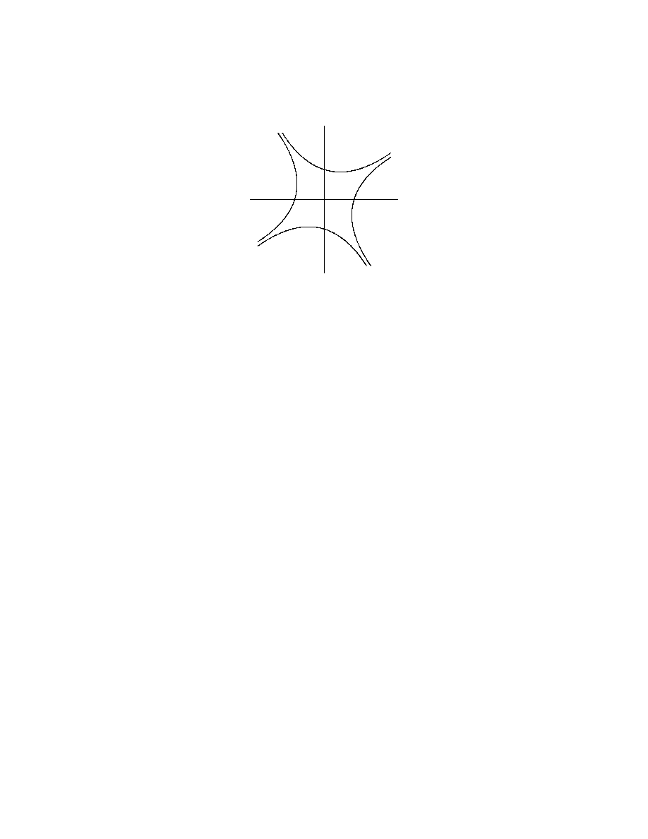
A more realistic example is given by a hyperbolic toral automor-
phism.
Example 1.2. Consider the map f :
x
y
7→
2 1
1 1
on R
2
. Figure
shows the eigenvectors in bold, and orbits of points being attracted to
the unstable direction.
Our purpose in these notes is to explore several questions.
(1) In which dynamical settings can these kind of portraits be use-
fully made?
(2) More generally, in which dynamical settings does the action
seen through a valuation tell you anything?
(3) Finally, can valuations in low-dimensional systems help us to
understand actions of higher-rank groups?
VALUATIONS AND HYPERBOLICITY IN DYNAMICS
3
3
+
J
J
J
J
^
J
J
J
J
J
J
J
J
]
J
J
J
J
Figure 2. A hyperbolic automorphism
2. S-integer dynamical systems
2.1. Definition and examples. The S-integer dynamical systems are
a very simple collection of dynamical systems which are the pieces from
which group automorphisms may be built up. Most of the material here
is taken from [
]. An excellent modern treatment of Tate’s thesis and
related material is the text of Ramakrishnan and Valenza, [
Let k be an A–field in the sense of Weil (that is, k is an algebraic
extension of the rational field Q or of F
q
(t) for some rational prime
q), and let P(k) denote the set of places of k. A place w ∈ P(k) is
finite if w contains only non–archimedean valuations and is infinite
otherwise (with one exception: for the case F
p
(t) the place given by
t
−1
is regarded as being an infinite place despite giving rise to a non–
archimedean valuation).
Example 2.1. For the case k
0
= Q or k
0
= F
q
(t), the places are
defined as follows.
The Rationals Q. The places of Q are in one–to–one correspondence
with the set of rational primes {2, 3, 5, 7, . . . } together with one addi-
tional place ∞ at infinity. The corresponding valuations are |r|
∞
= |r|
(the usual archimedean valuation), and for each p, |r|
p
= p
− ord
p
(r)
,
where ord
p
(r) is the (signed) multiplicity with which the rational prime
p divides the the rational r.
The Function Field F
q
(t). For F
q
(t) there are no archimedean
places. For each monic irreducible polynomial v(t) ∈ F
q
[t] there is a
distinct place v, with corresponding valuation given by
|f |
v
= q
− ord
v
(f )·deg(v)
,
where ord
v
(f ) is the signed multiplicity with which v divides the ra-
tional function f . There is one additional place given by v(t) = t
−1
,

4
THOMAS WARD
and this place will be called an infinite place even though the corre-
sponding valuation is non–archimedean. This ‘infinite’ place is defined
by |f |
∞
= q
− ord
t
(f (t
−1
))
.
Let k be a finite extension of k
0
. A place w ∈ P = P(k) is said to lie
above a place v of k
0
= Q or F
q
(t), denoted w|v, if | · |
w
rectricted to
the base field k
0
⊂ k coincides with | · |
v
. Denote by k
w
the (metric)
completion of k under the metric d
w
(x, y) = |x − y|
w
on k. The local
degree is defined by d
w
= [k
w
: (k
0
)
v
]. Choose a normalized valuation
| · |
w
corresponding to the place w to have
|x|
w
= |x|
d
w
/d
v
for each x ∈ k
0
\{0}, where d = [k : k
0
] is the global degree. With the
above normalizations we have the Artin product formula [
, p. 75]
(2.1)
Y
w∈P(k)
|x|
w
= 1
for all x ∈ k\{0}.
For each finite place w of k, the field k
w
is a local field, and the
maximal compact subring of k
w
is
r
w
= {x ∈ k : |x|
w
≤ 1}.
Elements of r
w
are called w–adic integers in k
w
. The group of units in
the ring r
w
is
r
∗
w
= {x ∈ k : |x|
w
= 1}.
Let P
∞
= P
∞
(k) denote the set of infinite places of k.
Definition 2.2. Let k be an A–field. Given an element ξ ∈ k
∗
, and any
set S ⊂ P(k)\P
∞
(k) with the property that |ξ|
w
≤ 1 for all w /
∈ S ∪P
∞
,
define a dynamical system (X, α) = (X
(k,S)
, α
(k,S,ξ)
) as follows. The
compact abelian group X is the dual group to the discrete countable
group of S–integers R
S
in k, defined by
R
S
= {x ∈ k : |x|
w
≤ 1 for all w /
∈ S ∪ P
∞
(k)}.
The continuous group endomorphism α : X → X is dual to the
monomorphism
b
α : R
S
→ R
S
defined by
b
α(x) = ξx.
Dynamical systems of the form (X
(k,S)
, α
(k,S,ξ)
) are called S–integer
dynamical systems. Following conventions from number theory, we
shall divide these into two classes: arithmetic systems when k is a
number field, and geometric when k has positive characteristic. To
clarify this definition – and to show how these systems connect with
previously studied ones – several examples follow.

VALUATIONS AND HYPERBOLICITY IN DYNAMICS
5
Example 2.3. (1) Let k = Q, S = ∅, and ξ = 2. Then
R
S
= {x ∈ Q : |x|
p
≤ 1 for all primes p} = Z,
so X = T and α is the circle doubling map.
(2) Let k = Q, S = {2}, and ξ = 2. Then
R
S
= {x ∈ Q : |x|
p
≤ 1 for all primes p 6= 2} = Z[
1
2
],
so X is the solenoid d
Z[
1
2
], and α is the automorphism of X dual to the
automorphism x 7→ 2x of R
S
. This is the natural invertible extension
of the circle doubling map [
, Sect. 2].
As pointed out in [
, Chap. 1 Example D], this dynamical system
is topologically conjugate to the system (Y, β) defined as follows. Let
D = {z ∈ C : |z| ≤ 1} and S
1
= {z ∈ C : |z| = 1}. Define a map
f : S
1
× D → S
1
× D by
f (z, ω) = (z
2
,
1
2
z +
1
4
ω).
Let Y =
T
n∈N
f
n
(S
1
× D) and let β be the map induced by f on Y .
Then there is a homeomorphism Y → X that intertwines the maps β
and α. For more details on this example and related “DE” (derived
from expanding) examples, see, [
, Section I.9]; for a thorough and
detailed treatment of this dyadic example see [
, Sect. 17.1].
(3) Let k = Q, S = {2, 3}, ξ =
3
2
. Then R
S
= Z[
1
6
], and α is the map
dual to multiplication by
3
2
on R
S
. This map has dense periodic points
by [
, Sect. 3] and has topological entropy log 3 by [
, Sect. 2].
(4) Let k = Q, S = {2, 3, 5, 7, 11, . . . }, and ξ =
3
2
. Then R
S
= Q and
α is the automorphism of the full solenoid b
Q dual to multiplication by
3
2
on Q. This map has only one periodic point for any period by [
Sect. 3] and has topological entropy log 3 by [
, Sect. 2].
(5) Let ξ be an algebraic integer, k = Q(ξ) and S = ∅. Then R
S
is
the ring of algebraic integers in k. Taking ξ =
√
2 − 1 + i
p
2
√
2 − 2
gives a non–expansive quasihyperbolic automorphism of the 4–torus as
pointed out in [
, Sect. 3]
(6) Let k = F
q
(t), S = ∅, and ξ = t.
Then R
S
= F
q
[t], and so
X = c
R
S
=
Q
∞
i=0
{0, 1, . . . , q − 1}. The map α is therefore the full
one–sided shift on q symbols.
(7) Let k = F
q
(t), S = {t}, and ξ = t. Recall that the valuation
corresponding to t is |f |
t
= q
− ord
t
(f )
, so |t|
t
= q
−1
. The ring of S–
integers is
R
S
= {f ∈ F
q
(t) : |f |
w
≤ 1 for all w 6= t, t
−1
} = F
q
[t
±1
].

6
THOMAS WARD
The dual of R
S
is then
Q
∞
−∞
{0, 1, . . . , q − 1}, and in this case α is the
full two–sided shift on q symbols.
(8) Let k = F
q
(t), S = {t}, and ξ = 1 + t. Then X is the two–sided
shift space on q symbols, and α is the cellular automaton defined by
(α(x))
k
= x
k
+ x
k+1
mod q.
(9) Let k = F
q
(t), S = {t, 1 + t}, and ξ = 1 + t. Then α is the invertible
extension of the cellular automaton in (8).
(10) Let α be an ergodic automorphism of a finite–dimensional torus.
For each subset S of the rational primes let Γ
S
= b
X ⊗
Z
Z[
1
S
]. Then
α defines an endomorphism α
S
: c
Γ
S
→ c
Γ
S
. Each α
S
has the same
entropy as α by [
] (and is therefore measurably isomorphic to α),
but they are all topologically distinct, so {α
S
} forms an uncountable
family of topological dynamical systems all measurably isomorphic to
each other.
(11) Not all toral endomorphisms are S–integer dynamical systems. Let
α
A
: T
n
→ T
n
be the toral endomorphism corresponding to the integer
matrix A ∈ M
n
(Z). Assume that the characteristic polynomial χ
A
of A
is irreducible, let λ have χ
A
(λ) = 0 and let a = (a
1
, . . . , a
n
)
t
be a vector
in Q(λ)
n
with Aa = λa with the property that a = a
1
R
λ
+ · · · + a
n
R
λ
is an ideal in the ring R
λ
= Z[λ]. Two ideals determined in this way
from the same matrix belong to the same ideal class by [
, Th. 2].
Lemma 2.4. The toral endomorphism α is topologically conjugate to
the S–integer dynamical system given by k = Q(λ), ξ = λ, S = ∅ if
and only if a defines a trivial element in the ideal class group of R
λ
.
Proof. Let B be the companion matrix to the polynomial χ
A
. Then
there is an isomorphism from X
(k,S)
, α
(k,ξ,S)
to (T
n
, α
B
). If a defines
a trivial element in the ideal class group of R
λ
, then by [
], there is a
matrix S ∈ GL
n
(Z) such that A = SBS
−1
, so there is an isomorphism
from (T
n
, α
B
) to (T
n
, α
A
).
Conversely, let θ : (T
n
, α
A
) → X
(k,S)
, α
(k,ξ,S)
be a topological con-
jugacy. Let H
1
denote the first ˇ
Cech homology functor with coeffi-
cients in T; H
1
sends any diagram of solenoids and endomorphisms
to an isomorphic diagram by [
, Lemma 6.3]. Then H
1
(θ) defines
an isomorphism from (T
n
, α
A
) to X
(k,S)
, α
(k,ξ,S)
; since X
(k,S)
is an n–
dimensional torus, α
(k,ξ,S)
corresponds to some matrix C ∈ M
n
(Z), and
this isomorphism is given by a matrix S ∈ GL
n
(Z) with A = SCS
−1
.
It follows by [
] that a defines a trivial element in the ideal class group
of R
λ
.

VALUATIONS AND HYPERBOLICITY IN DYNAMICS
7
2.2. Background on adeles. In this section we assemble some basic
facts about the ring R
S
. For the case S = ∅ most of this is straight-
forward. At the opposite extreme, when S contains all finite places (so
R
S
= k), the adelic constructions of [
, Chap. IV] show how to cover
the group X
(k,S)
. In the intermediate case, straightforward modifica-
tions of Weil’s arguments are needed. The construction is also given
in Tate’s thesis, and we indicate below how to read off the results we
shall need from this.
Fix an A–field k and a set S of finite places of k.
Definition 2.5. The S–adele ring of k is the ring
k
A
(S) =
(
x = (x
ν
) ∈
Y
ν∈S∪P
∞
k
ν
: |x
ν
|
ν
≤ 1 for all but finitely many ν
)
,
with the topology induced by the following property. For each finite
set S
0
⊂ S, the locally compact subring k
S
0
A
⊂ k
A
(S) defined by
k
S
0
A
=
Y
ν∈S
0
∪P
∞
k
ν
×
Y
ν∈S\S
0
r
ν
(with the product topology) is an open subring of k
A
(S), and a fun-
damental system of open neighbourhoods of 0 in the additive group of
k
A
(S) is given by a fundamental system of neighbourhoods of 0 in any
one of the subrings k
S
0
A
.
Notice that k
A
(S) is locally compact since each r
ν
is compact.
Define a map ∆ : R
S
→ k
A
(S) by ∆(x) = (x, x, x, . . . ). This map is
a well–defined ring homomorphism: notice that for α ∈ R
S
, |α|
ν
≤ 1
for all but finitely many ν by [
, Th. III.1.3].
In [
], Tate introduces the notion of an abstract restricted direct
product, under the hypothesis that P (= S ∪ P
∞
) is an arbitrary count-
able set of indices (places). Let G
P
(= k
ν
) be a locally compact abelian
group for P ∈ P , and for all but finitely many P, let H
P
(= r
ν
) be an
open compact subgroup of G
P
. The restricted direct product is defined
as
G(P ) =
(
g = (g
P
) ∈
Y
P∈P
G
P
: g
P
∈ H
P
for all but finitely many P
)
,
a locally compact abelian topological group. We topologise G(P ) by
choosing a fundamental system of neighbourhoods of 1 in G(P ) of the
form N =
Q
P∈P
N
P
, where each N
P
is a neighbourhood of 1 in G
P
and
N
P
= H
P
for all but finitely many P, which accords with the topology
in Definition

8
THOMAS WARD
The key results proved in [
, Lem. 3.2.2, Th. 3.2.1] are the follow-
ing.
(1) ∆(R
S
) is discrete in k
A
(S) and k
A
(S)/∆(R
S
) is compact,
(2) R
⊥
S
∼
= R
S
, \
k
A
(S) ∼
= k
A
(S) and so k
A
(S)/∆(R
S
) ∼
= ˆ
R
S
where S is an arbitrary set of finite places of an A–field k. We collect
these remarks in the following Theorem, which is an extension of one
of the “Main Theorems” in [
, Chap. IV, Sect. 2] to arbitrary sets of
places.
Theorem 2.6. The map ∆ : R
S
→ k
A
(S) embeds R
S
as a discrete
cocompact subring in the S–adele ring of k. There is an isomorphism
between the S–adele ring k
A
(S) and itself, which induces an isomor-
phism between c
R
S
and k
A
(S)/∆(R
S
).
Remark 2.7. The S–adele ring k
A
(S) covering the dynamical system
(X
(k,S)
, α
(k,S,ξ)
) gives a complete local portrait of the hyperbolicity. A
neighbourhood of the identity in X
(k,S)
is isometric to a neighbourhood
of the identity in k
A
(S). The map α
(k,S,ξ)
under this isometry acts
on each quasi–factor k
ν
by multiplication, dilating the metric on that
quasi–factor by |ξ|
ν
. If S is infinite, then the local action is an isometry
on all but finitely many quasi–factors, making such systems very far
from hyperbolic ones.
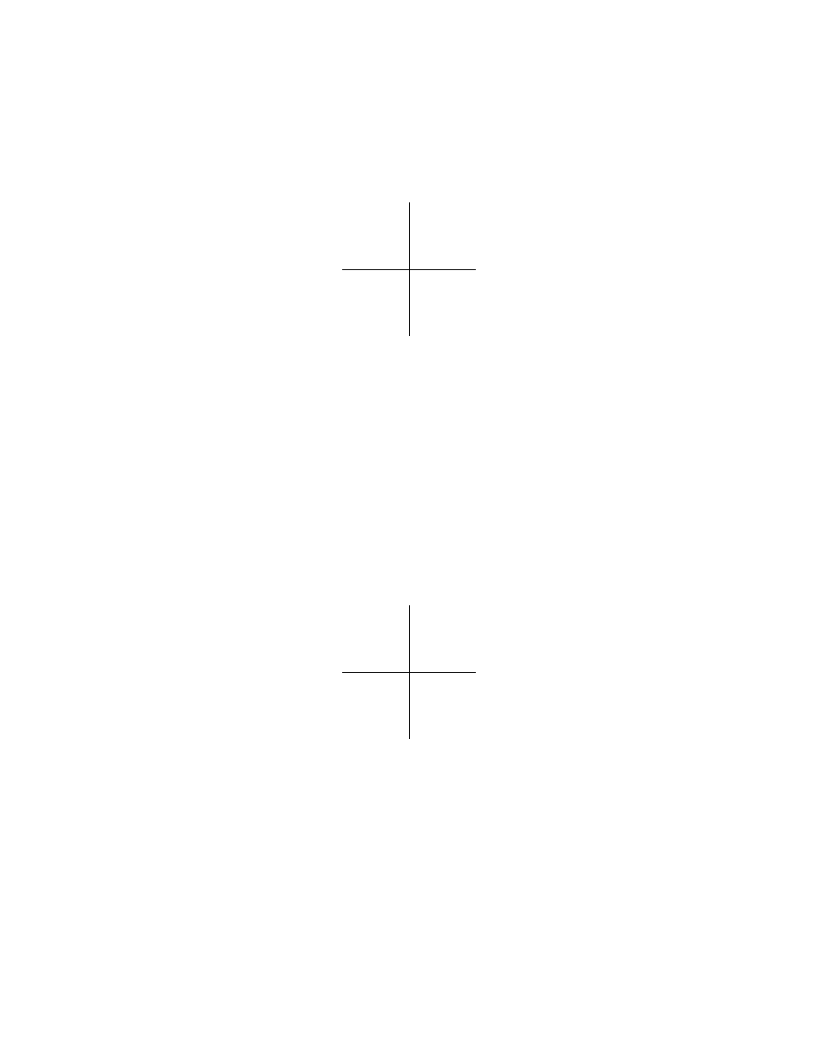
2.3. Adelic covering space. We first recall how covering spaces arise
for familiar maps. If f : T → T is the doubling map x 7→ 2x mod 1
on the additive circle, then the cover π : R → T lifts the map to
˜
f : R → R. Figure
shows the lifted map: notice that the projection
π is a local isometry. The import of Section
is that the same thing
T
T
R
R
-
α
-
˜
α
?
π
π
?
Figure 3. Lifting the circle doubling map
happens for any S-integer dynamical system.
Example 2.8. Let α be the S–integer dynamical system corresponding
to k = F
p
(t), S = {t} and ξ = t (so the corresponding dynamical
system is the full p-shift). The covering space is the product k
∞
×
k
v
where v is the valuation corresponding to t and ∞ the valuation
VALUATIONS AND HYPERBOLICITY IN DYNAMICS
9
corresponding to t
−1
. The local hyperbolicity portrait in the covering
space is shown in Figure
6
×|t|
t
−1
= p
?
×|t|
t
= p
−1
-
Figure 4.
Multiplication by t is hyperbolic for S = {t}
The system is hyperbolic, which shows up in having extremely reg-
ular properties (for example, the dynamical zeta function is rational).
Example 2.9. A non-hyperbolic additive cellular automaton is given
by choosing k = F
p
(t), S = {t} and ξ = 1 + t. This is the additive
cellular automata with local rule given by
f (x
0
, x
1
) = x
0
+ x
1
.
If p = 2 this is ‘rule 102’ in the standard description of cellular au-
tomata with radius 1. The covering space is the same product. The
local hyperbolicity portrait is shown in Figure
, which indicates why
this system is non–hyperbolic.
6
×|1 + t|
t
−1
= p
?
×|1 + t|
t
= 1
Figure 5.
Local effect of multiplication by 1 + t
The non-hyperbolicity makes the dynamics extremely complicated:
the direction in which the map acts likes an isometry behaves like a
sort of rotation, destroying some (but not all) periodic points.
The final example is a connected group automorphism.
Example 2.10. Let k = Q, S = {2, 3} and ξ = 2. This system is
an isometric extension of the invertible extension of the circle doubling
map. The covering space is R × Q
2
× Q
3
.
10
THOMAS WARD
6
×|2|
∞
?
×|2|
3
= 1
+
3
×|2|
2
Figure 6.
Local effect of multiplying by 2 on d
Z[
1
6
]
2.4. Topological entropy. For any automorphism α : X → X of
a compact metrizable group X, the topological entropy h(α) may be
defined in several different ways. The most convenient formulation is
that of Bowen [
], where the topological entropy is expressed as a local
rate of volume growth.
Definition 2.11. The topological entropy of the compact group auto-
morphism α : X → X is defined to be
h
Bowen
(α) = lim
&0
lim sup
n→∞
−
1
n
log µ
n−1
\
k=0
α
−k
B
(α
k
x)
!
,
where x is any point, µ is Haar measure, and B
denotes the metric
open ball around x.
Bowen [
, Prop. 7] is that
h(α) = h
Bowen
(α).
This gives a very straightforward way to compute the entropy of auto-
morphisms of solenoids (compact, connected, finite-dimensional groups)
– this entropy was computed originally by Yuzvinskii [
], and then a
much simpler proof using Bowen’s formulation and the adelic covering
space was given in [
] for the solenoid case. The geometric
case, which includes certain cellular automata is similar (see [
Theorem 2.12. The topological entropy of an S–integer system is
given by
(2.2)
h(α
(k,S,ξ)
) =
X
w∈S∪P
∞
(k)
log
+
|ξ|
w
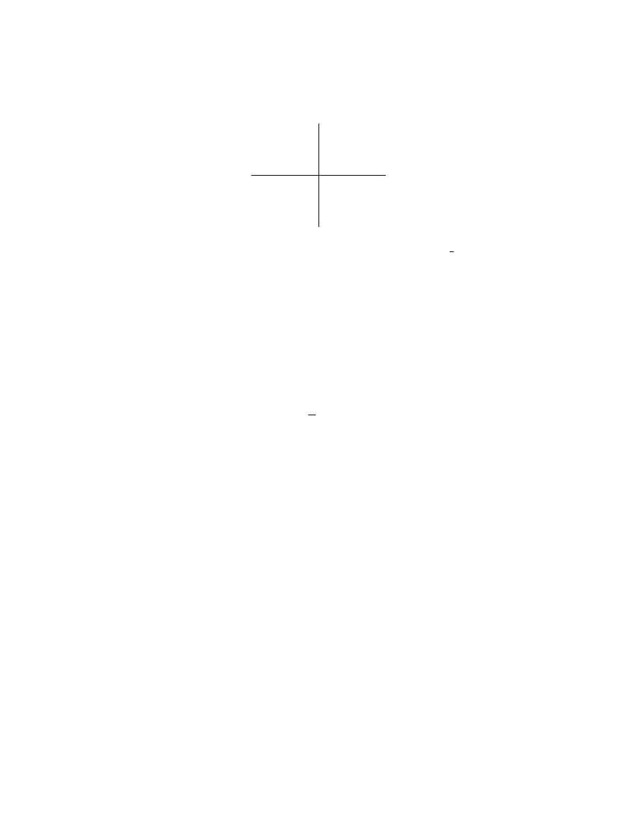
Proof. The proof is sketched for a simple case. Assume that the field k
has positive characteristic (so all the places are non-Archimedean) and

VALUATIONS AND HYPERBOLICITY IN DYNAMICS
11
k
s
/∆(R
S
) ∼
= X
S
-
α
(S,ξ)
X
S
∼
= k
s
/∆(R
S
)
?
?
p
p
k
S
k
S
-
˜
α
Figure 7. Adelic covering space
assume that the set S is finite (so the topology on the S-adele ring is
simple the product topology).
Using Section
the group R
S
embeds as a discrete subgroup of
Q
ν∈S∪P
∞
k
ν
with compact quotient, and there is a map p : k
S
→
k
s
/∆(R
S
); Theorem
means that there is a commutative diagram
expressing the adelic covering space k
S
, shown in Figure
in which the map p is a local isometry and ˜
α denotes multiplication
by ξ in each coordinate.
It follows by [
, Th. 9, 20] that
(2.3)
h(α) = h( ˜
α) = lim
&0
lim sup
n→∞
−
1
n
log µ
n−1
\
j=0
˜
α
−j
(B
)
!
where B
is the metric open ball of radius around the identity, µ
is Haar measure on the locally compact group
Q
ν∈S∪P
∞
k
ν
, and ˜
α
is the lifted map (x
ν
)
ν∈S∪P
∞
7→ (ξx
ν
)
ν∈S∪P
∞
on the covering space
Q
ν∈S∪P
∞
k
ν
.
Since S is finite, we may use the max metric on
Q
ν∈S∪P
∞
k
ν
. It
follows that
B
= {(x
ν
) : |x|
ν
< ∀ ν ∈ S ∪ P
∞
}.
Now the covering map from
Q
ν∈S∪P
∞
k
ν
onto X
S
gives a local portrait
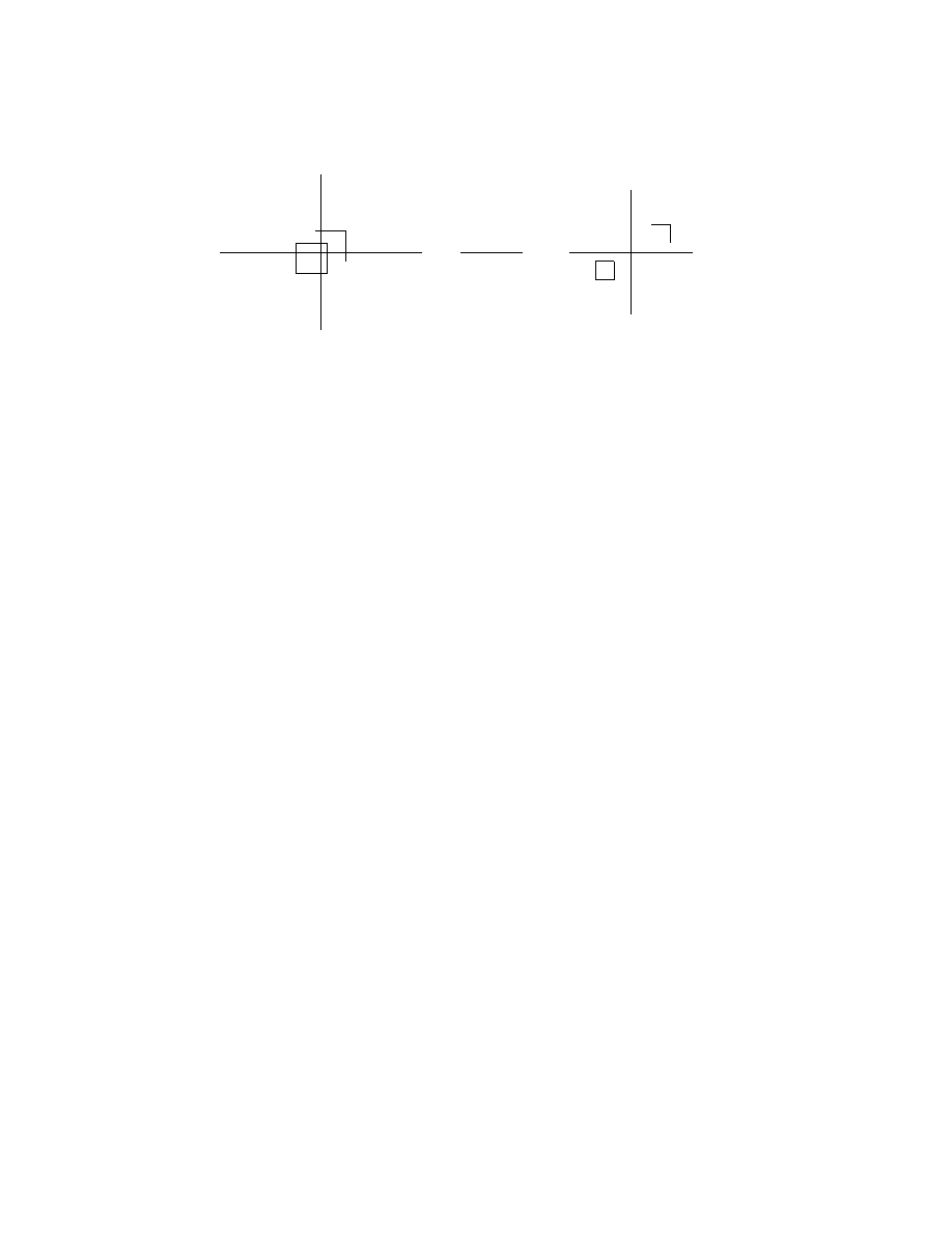
of the hyperbolicity.
For example, if S ∪ P
∞
= {ν
1
, ν
2
, ν
3
} say, and |ξ|
ν
1
> 1, |ξ|
ν
2
> 1,
|ξ|
ν
3
< 1 then the local dynamics in a neighbourhood of the identity
in X
S
is illustrated in Figure
. The box B
is transformed under ˜
α
−1
(multiplication by ξ
−1
) into a squashed box with sides of length 2|ξ|
−1
ν
1
,
2|ξ|
−1
ν
2
, 2|ξ|
−1
ν
3
in the directions corresponding to ν
1
, ν
2
, ν
3
respectively.
In the covering space the effect of multiplying the box B
by ξ
−1
gives
˜
α
−j
(B
) = {(x
ν
) : |ξ
j
x|
ν
< ∀ ν ∈ S ∪ P
∞
}
= {(x
ν
) : |x|
ν
< /|ξ|
j
ν
∀ ν ∈ S ∪ P
∞
}.
12
THOMAS WARD
6
×|ξ|
ν
1
?
-
×|ξ|
ν
2
+
3
×|ξ|
ν
3
B
-
˜
α
−1
k
ν
2
k
ν
1
k
ν
3
Figure 8.
Multiplying B
by ξ
−1
for S ∪ P
∞
= {ν
1
, ν
2
, ν
3
}
Thus the set
D(n, ) =
n−1
\
j=0
˜
α
−j
(B
)
is a ‘box’ with one side for each term ν ∈ S ∪ P
∞
, and the ‘length’ of
each side is
(2.4)
min{, /|ξ|
ν
, /|ξ|
2
ν
, . . . , /|ξ|
n−1
ν
} =
if |ξ|
ν
≤ 1,
/|ξ|
n−1
ν
if |ξ|
ν
> 1.
It follows that
µ (D(n, )) =
|S∪P
∞
|
·
Y
ν:|ξ|
ν
>1
|ξ|
n−1
ν
−1
,
which when substituted into (
2.5. Dynamical properties. Recall the following standard criterion
for ergodicity of compact group automorphisms.
Theorem 2.13. If X is a compact metrizable abelian group and α :
X → X is a surjective continuous endomorphism then Haar measure
is ergodic for T if and only if the trivial character γ ≡ 1 is the only
γ ∈ ˆ
X satisfying γ ◦ T
n
= γ for some n > 0.
Proof. See [
, Th. 1].
Corollary 2.14. Let (X, α) = (X
(k,S)
, α
(k,S,ξ)
) be an S–integer dynam-
ical system. Then α is ergodic if and only if ξ is not a root of unity.
It follows that in the geometric case α is ergodic if and only if ξ /
∈ F
∗
p
.
Proof. The map α is non–ergodic if and only if there is a r ∈ R
S
\{0}
with ξ
m
r = r for some m 6= 0. This is possible in a field if and only if
ξ is a unit root.

VALUATIONS AND HYPERBOLICITY IN DYNAMICS
13
Recall that a continuous map α : (X, d) → (X, d) is forwardly ex-
pansive if there is a constant δ > 0 such that for each pair x 6= y ∈ X
there is some n ∈ N with d(α
n
x, α
n
y) > δ. A homeomorphism β :
(X, d) → (X, d) is expansive if there is a constant δ > 0 such that for
each pair x 6= y ∈ X there is some n ∈ Z with d(β
n
x, β
n
y) > δ. Home-
omorphisms can only be forwardly expansive on finite metric spaces –
this observation seems to have been first made in the Ph.D. thesis of
Schwartzman; a proof is in [
Theorem 2.15. Let K be a non–discrete field complete with respect to
a valuation | · |, and let ¯
K denote the algebraic closure of K with the
uniquely extended absolute value from K. Let E be a finite dimensional
vector space over K, and let u be an automorphism of E. Then u is
expansive if and only if |λ| 6= 1 for each eigenvalue λ of u in ¯
K.
Proof. See Eisenberg’s paper [
, Th. 3].
There is an infinite-dimensional analogue of Eisenberg’s result – see
Corollary 2.16. Let (X, α) = (X
(k,S)
, α
(k,S,ξ)
) be an S–integer dynam-
ical system. Then α is expansive if and only if S ∪ P
∞
⊆ {ν ≤ ∞ :
|ξ|
ν
6= 1}.
Proof. Recall that there is a local isometry between k
A
(S) and X, so
it is enough to check expansiveness of the lifted map on k
A
(S). Here
Eisenberg’s criterion in Theorem
applies to each of the (finitely
many) indicated quasifactors.
Remark 2.17. Corollary
is a generalisation of [
, Prop. 7.2]
where Schmidt considers k to be a number field and S = {ν < ∞ :
|ξ|
ν
6= 1}.
2.6. Periodic points. One of the remarkable features of S-integer
systems is that there is an exact formula for the number of periodic
points. To see where this comes from, go back to the circle doubling
map, α : T → T. Finding the points of period n under this map
amounts to solving the equation (2
n
− 1)x = 0 mod 1 on T. One way to
count solutions to this equation is to use the covering space π : R → T
again: fix a fundamental domain F for π (this could be [0, 1) say –
but it does not really matter as long as it is a measurable set) and
consider the image of F under ×(2
n
− 1) in the covering space: write
G = (2
n
−1)F . I claim that the set G contains exactly (2
n
−1) integers,
and the pre-image of each of these under multiplication by (2
n
− 1)
gives a unique point of period n. It follows that the number of points

14
THOMAS WARD
of period n is equal to the amount by which the map x 7→ (2
n
− 1)x
scales Lebesgue measure on R.
Let Γ be a discrete cocompact subgroup of a locally compact abelian
group X. A fundamental domain F of X modulo Γ is a full (measur-
able) set of coset representatives of Γ in X. Denote by µ the Haar
measure on X normalised to give µ(F ) = 1. Let ˜
A : X → X be a con-
tinuous surjective mapping with ˜
A(Γ) ⊂ Γ, and let A : X/Γ → X/Γ
be the induced map on the quotient space.
Lemma 2.18. If ker A is discrete, then
mod
X
( ˜
A) = | ker A|.
Proof. Since Γ is discrete in X, a fundamental domain F may be chosen
so that there exists a neighbourhood U (0
X
) of the identity 0
X
∈ X with
U (0
X
) ⊂ F . The finiteness of | ker A| follows from the fact that X/Γ
is compact. So for a sufficiently small neighbourhood V (0
X/Γ
) of the
identity 0
X/Γ
∈ X/Γ,
A
−1
V (0
X/Γ
) =
[
i=1,...,| ker A|
V
i
,
where each V
i
is a neighbourhood of a point in the set A
−1
(0
X/Γ
) and
their union is disjoint. Since A is measure–preserving, µ A
−1
V (0
X/Γ
)
=
µ V (0
X/Γ
)
. Once again using the discreteness of Γ in X we have that
X is locally isomorphic to X/Γ. This means that, assuming the neigh-
bourhoods U (0
X
) and V (0
X/Γ
) are small enough, π|
U (0
X
)
is a homeo-
morphism between U (0
X
) and V (0
X/Γ
). Thus we have
µ
˜
AU (0
X
)
= µ AV (0
X/Γ
)
= | ker A|µ V (0
X/Γ
)
= | ker A|µ (U (0
X
))
which proves the Lemma. Furthermore, since U (0
X
) ⊂ F , µ( ˜
AF ) =
| ker A|.
Lemma 2.19. Let (X, α) = (X
(k,S)
, α
(k,S,ξ)
) be an S–integer dynamical
system. Then the number of points of period n ≥ 1 is finite if α is
ergodic, and
| Per
n
(α)| =
Y
ν∈S∪P
∞
|ξ
n
− 1|
ν
.

VALUATIONS AND HYPERBOLICITY IN DYNAMICS
15
Proof. A fundamental domain of k
A
(S) modulo k is a set
F =
[0, 1)
d
×
Q
ν∈S
r
ν
if k is a number field with d = [k : Q],
Finite ×
Q
ν∈S∪P
∞
r
ν
otherwise.
The set F is measurable. For each ν ∈ S ∪ P
∞
, let µ
ν
denote a Haar
measure on k
ν
normalised to have µ
ν
(r
ν
) = 1 for all but finitely many
ν. Then the product measure µ =
Q
ν∈S∪P
∞
µ
ν
is well defined and is a
Haar measure on k
A
(S). Set A = α
n
− I, X = k
A
(S) and Γ = ∆(R
S
),
then ergodicity implies that ker A is discrete in ˆ
R
S
and by Lemma
we have
| Per
n
(α)| = | ker(α
n
− 1)| = µ (( ˜
α
n
− 1)F ) =
Y
ν∈S∪P
∞
|ξ
n
− 1|
ν
.
2.7. Growth rates. Any expansive map α must have
(2.5)
lim sup
n→∞
1
n
log Per
n
(α) ≤ h(α)
but many natural systems have a much stronger property.
Theorem 2.20. If α : X → X is an expansive automorphism of a
compact connected group, then
lim
n→∞
1
n
log Per
n
(α) = h(α).
In fact the same is true of ergodic automorphisms under a finiteness
condition, but this is much more subtle (see below).
It is clear from Lemma
and Theorem
that for S–integer
dynamical systems we always have
lim inf
n→∞
1
n
log Per
n
(α) ≤ lim sup
n→∞
1
n
log Per
n
(α) ≤ h(α) < ∞.
A useful measure of the regularity of periodic points is the dynamical
zeta function of α,
(2.6)
ζ
α
(z) = exp
∞
X
n=1
Per
n
(α)
z
n
n
,
a (formal) power series defined whenever Per
n
(α) is finite for all n ≥ 1.
By Hadamard, if (
) actually defines a holomorphic
function in the disk of radius e
−h(α)
about the origin.
Several Diophantine issues come up in trying to extend Theorem
. In order to see what is involved in finding the growth rate of
periodic points for S-integer systems, consider the following examples.

16
THOMAS WARD
Example 2.21. Let ξ =
√
2 − 1 + i
p
2
√
2 − 2, k = Q(ξ), S = ∅. Then
R
S
= Z + ξZ + ξ
2
Z + ξ
3
Z
∼
= Z
4
, so X
(k,S)
is the 4-torus T
4
, and the
action of α
(k,ξ,S)
is isomorphic to the action of the matrix
A =
0
1
0
0
0
0
1
0
0
0
0
1
−1 −4 2 −4
with eigenvalues λ
1
=
√
2 − 1 + i
p
2
√
2 − 2 ≈ .414 + .910i, λ
2
=
√
2 − 1 − i
p
2
√
2 − 2 ≈ .414 − .910i, λ
3
≈ −.217 and λ
4
≈ −4.612. The
formula for the periodic points gives
Per
n
(A) = det(A
n
− I) =
4
Y
j=1
|λ
h
j
− 1|.
The last two terms are fine: it is clear that
lim
n→∞
1
n
log |λ
h
3
− 1| × |λ
h
4
− 1|
= log |λ
4
| = h(α).
The problem is with the first two terms: |λ
1
| = |λ
2
| = 1, but neither are
unit roots. This means that, for example |λ
n
1
− 1| gets arbitrarily small
for certain values of n (the argument of λ
1
is not a rational multiple
of π, so multiplication by λ
1
behaves like an irrational circle rotation
with dense orbits). This problem is discussed in [
], where it is shown
to be equivalent to a problem solved by Gel
0
fond in [
]. Since it is
better-known, we will use Baker’s stronger result.
Lemma 2.22. [baker’s theorem] If λ is an algebraic number that
is not a root of unity, then there exist constants A and B for which
(2.7)
|λ
n
− 1| >
A
n
B
.
It follows at once that the other two terms do not contribute anything
to the logarithmic growth rate:
lim
n→∞
1
n
log |λ
h
1
− 1| × |λ
h
2
− 1|
= 0.
We conclude that
lim
n→∞
1
n
log Per
n
(α) = h(α)
for this non-expansive toral automorphism.
Example 2.23. If k = Q, S = {2, 3} and ξ = 2, then
Per
n
= (2
n
− 1) × |2
n
− 1|
3
,

VALUATIONS AND HYPERBOLICITY IN DYNAMICS
17
so the growth rate of periodic points presents a similar problem. The
first term is fine: (1/n) log |2
n
− 1| → log 2, but the second term is less
clear. There certainly is a sequence (n
j
) for which |2
n
j
− 1|
3
→ 0, the
question is how fast must such a sequence grow?
Lemma 2.24. Let k be a an A-field of characteristic zero, fix ξ not a
unit, and let T be any finite subset of the finite places of k. Then there
are constants A, B > 0 for which
1 ≥
Y
v∈T
|ξ
n
− 1|
v
≥
A
n
B
.
This is not a deep result at all, and implies for example that
lim
n→∞
1
n
log |2
n
− 1|
3
= 0,
which shows that for this system also
lim
n→∞
1
n
log Per
n
(α) = h(α).
Similar reasoning gives the following theorem.
Theorem 2.25. Let (X, α) = (X
(k,S)
, α
(k,S,ξ)
) be an ergodic arithmetic
S–integer dynamical system with S finite. Then the growth rate of the
number of periodic points exists and is given by
(2.8)
lim
n→∞
1
n
log Per
n
(α) = h(α).
On the other hand, for most S-integer systems the dynamical zeta
function is not rational (or even algebraic).
Example 2.26. The geometric case is very different: it is clear that
property (
) does not hold for non-hyperbolic linear cellular automata
for example. Example
with k = F
2
(t), S = {t} and ξ = 1+t already
shows some of the difficulties. The entropy is log 2, and Lemma
says that
|F
n
(α)| = |(t + 1)
n
− 1|
∞
|(t + 1)
n
− 1|
t
= p
n
t
n
+
n
1
t
n−1
+ . . . +
n
n − 1
t
t
.
We claim that the set of limit points of
1
n
log |F
n
(α)|
∞
n=1
is
1 −
1
q
h(α) : q ∈ N, p 6 |q
∪ {h(α)}.

18
THOMAS WARD
This is seen as follows: write n = qp
ord
p
(n)
where p 6 |q then
|F
n
(α)| = |(t + 1)
n
− 1|
∞
|(t + 1)
q
− 1|
t
= p
n
p
−p
ordp(n)
since p 6 |q
= p
n
(
1−
1
q
).
So for a sequence n
j
→ ∞ with n
j
/p
ord
p
(n
j
)
= q for a fixed q, p 6 |q,
lim
ord
p
(n
j
)→∞
1
n
j
log |F
n
j
(α)| =
1 −
1
q
log p.
Also, p
+
(α) = h(α) is obtained by letting n → ∞ through the numbers
which are coprime to p.
Similar reasoning gives the following general result.
Theorem 2.27. Let (X, α) = (X
(k,S)
, α
(k,S,ξ)
) be an ergodic geometric
S–integer dynamical system with S finite. Then
lim sup
n→∞
1
n
log Per
n
(α) = h(α),
and (usually) the set
1
n
log Per
n
(α)
has infinitely many other limit
points.
Given that elements of S destroy periodic points, an interesting ques-
tion is to ask if S can be infinite while still having many periodic points.
It turns out that this is so in a very strong sense – see Section
. Be-
fore that, I will describe an example due to Chothi [
]. Let k = Q and
suppose ξ is a non–zero integer. Recall that ξ is said to be a primitive
root modulo a prime p if and only if the residue classes modulo p of
ξ, ξ
2
, . . . , ξ
p−1
≡ 1 are all distinct. The number of primitive roots mod-
ulo p is φ(p − 1), where φ is the Euler function. For example, 2 is not a
primitive root modulo 7 since 2
3
≡ 1(mod 7). In 1927 Artin made the
following conjecture: if a is neither a square nor −1, then there exist
infinitely many primes such that a is a primitive root modulo p. So, if
we choose ξ ∈ Z to be neither a square nor −1 and define S to be the
set of places |.|
p
for which ξ is a primitive root modulo p, then Artin’s
conjecture implies that S is infinite. Let α be the endomorphism of ˆ
R
S
dual to multiplication by ξ on R
S
.
Theorem 2.28. If Artin’s conjecture holds for ξ then p
+
(α) = h(α).
Proof. Since |ξ
n
− 1|
p
= 1 if and only if p − 1 6 |n for each p ∈ S, we
have
1
n
log |F
n
(α)| =
1
n
log |ξ
n
− 1|
∞
+
1
n
X
p∈S:p−1|n
log |ξ
n
− 1|
p
.

VALUATIONS AND HYPERBOLICITY IN DYNAMICS
19
So by letting n → ∞ through all the prime numbers, we get
lim sup
n→∞
1
n
log |F
n
(α)| = log |ξ| = h(α).
Theorem 2.29. [heath–brown] There are infinitely many primes p
with either 2 or 3 or 5 as a primitive root.
Proof. Heath–Brown [
] proves that, with the exception of at most
two primes the following is true: for each prime q there are infinitely
many primes p with q a primitive root modulo p.
Corollary 2.30. There exist non–expansive systems ( ˆ
R
S
, α) with S
infinite such that
lim sup
n→∞
1
n
log Per
n
(α) = h(α) > 0.
These dynamical systems have the remarkable property that on the
one hand they mimic hyperbolic behaviour (lim sup
n→∞
1
n
log Per
n
(α) =
h(α)), while on the other they have infinitely many directions in which
they behave as isometries.
Theorem
will appear again in connection with geometric systems
(cf. Theorem
2.8. Typical group automorphisms. It is not clear whether it makes
sense to speak of a ‘typical’ or ‘generic’ compact group automorphism.
For one thing, it is not known what values the most obvious global
invariant, the topological entropy, takes on. In order to explain this
first difficulty, recall that the Mahler measure of a polynomial f ∈ Z[x]
is defined to be
m(f ) =
Z
1
0
log |f (e
2πis
)|ds.
An application of Jensen’s formula shows that if ξ is an algebraic num-
ber with minimal polynomial f , and S = ∅, then the entropy of the
associated S-integer system is m(f ). This appearance of Mahler mea-
sures as entropies also arises for higher-rank actions, which we will see
again later.
Problem 2.31. [lehmer’s problem] Is 0 a cluster point of
{m(f ) | f ∈ Z[x]}?

20
THOMAS WARD
This problem arose in Lehmer’s paper [
] of 1933 and seems to be
very deep. For an extended discussion of what is know about it, see [
and [
]. Mahler measures (for polynomials in several variable) have
arisen in several areas of mathematics, including ergodic theory [
number theory [
] and knot
theory [
The connection between Lehmer’s problem and the problem of de-
scribing all compact group automorphisms is provided by a result due
to Lind [
] (the same result holds in higher-rank also: see [
Theorem 2.32. The set of possible entropies of compact group auto-
morphisms is all of [0, ∞] if the answer to Lehmer’s problem is ‘yes’,
and is the countable set {m(f ) | f ∈ Z[x]} if the answer is ‘no’.
Even after choosing a fixed entropy, it is not clear how to describe
all the group automorphisms with that entropy. So we focus on a
much simpler setting: for fixed k and ξ, can anything be said about
the dynamics of α
(k,S,ξ)
for a ‘typical’ set S? What (little) is known is
described in the papers [
]. Here we simply examine two
examples that illustrate some of the difficulties. For the first example,
we make the unwarranted assumption that there are infinitely many
Mersenne primes.
Example 2.33. Let k = Q, ξ = 2, and parametrize the possible
sets S as follows: identify S ⊂ {3, 5, 7, 11, . . . } with a unique point
in {0, 1}
N
in the obvious way, and place the iid (1/2, 1/2)-measure on
this set. Assume that n
1
< n
2
< . . . is a sequence of primes for which
p
j
= 2
n
j
− 1 is prime. Now for almost every S, there is a sequence
j
1
< j
2
< . . . of primes with p
j
k
∈ S for all k. Now for any such S,
Per
j
k
(α
(Q,2,S)
) = |2
j
k
− 1| × |2
j
k
− 1|
p
jk
= 1,
so
lim inf
n→∞
1
n
log Per(α
(Q,2,S)
) = 0
almost surely. On the other hand, for almost every S there is a sequence
`
1
< `
2
< . . . with p
`
k
/
∈ S for all k. Now for any such S,
Per
`
k
(α
(Q,2,S)
) = |2
`
k
− 1|,
so
lim sup
n→∞
1
n
log Per(α
(Q,2,S)
) = log 2
almost surely.

VALUATIONS AND HYPERBOLICITY IN DYNAMICS
21
In fact the full Mersenne prime conjecture is not needed to reach the
conclusions of Example
: all that is needed is the weaker assump-
tion that
P
∞
n=1
2
−ω(2
n
−1)
= ∞, where ω(N ) is the number of primes
dividing N .
What can be said without making any assumptions?
Theorem 2.34. Let k = Q, ξ = 2. Then for almost every S
lim sup
n→∞
1
n
log Per
n
(α) ≥
1
2
log 2.
Proof. This is proved in three steps: the first is to show that the set of
S for which the upper limit is positive must have positive measure. The
second is to show that there is an ergodic transformation on the set of
S’s that preserves the upper limit, so that there must be a set of full
measure on which it is constant (and positive by the first part). The
third is to use an involution on the set of S’s and the Artin-Whaples
product formula to see that this upper limit must be at least half the
entropy.
Step 1: Let
E =
S | lim sup
n→∞
1
n
log Per
n
α
(Q,S,2)
> 0
;
I claim that E has positive measure. Let ¯
S = S ∪ {∞}, and assume
that E has zero measure. Then for almost every S,
(2.9)
lim
n→∞
1
n
log
Y
v∈ ¯
S
|2
n
− 1|
v
= 0.
On the other hand, we know that
(2.10)
lim
n→∞
1
n
log
Y
v=2,∞
|2
n
− 1| = log 2 > 0.
Now let ¯
S
∗
= {v | v /
∈ S} ∪ {2, ∞}. By the product formula,
(2.11)
Y
v∈ ¯
S
|η|
v
×
Y
v∈ ¯
S∗
|η|
v
= |2
n
− 1| × |2
n
− 1|
2
= |2
n
− 1|.
The three equations (
) together imply that for almost
every S,
(2.12)
lim
n→∞
1
n
log
Y
v∈ ¯
S
|2
n
− 1|
v
= log 2 > 0,
which contradicts (
). We deduce that E must have positive measure.
Step 2: Notice that the set E certainly does not contain the set S =
{2, 3, 5, 7, . . . } of all primes (corresponding to the point (1, 1, 1, . . . ) ∈

22
THOMAS WARD
{0, 1}
N
). So if we write the primes as {p
1
, p
2
, . . . }, any member of E
looks like
S = {p
n(1)
, p
n(2)
, p
n(3)
, . . . };
with n(1) < n(2) < n(3) < . . . and n(j) = j only finitely often: for
j = 1, . . . , r say. Then define a map V on the set of all S by
V (S) = {ν
m(1)
, ν
m(2)
, ν
m(3)
, . . . };
where m(1) = n(r) + 1, m(`) = n(r + ` − 1) for ` ≥ 2 if n(1) = 1, and
m(1) = 1, m(`) = n(` − 1) for ` ≥ 2 if n(1) > 1. If sets S are thought
of as sequences of 0’s and 1’s, then V is the add-and-carry odometer,
ergodic with respect to the (1/2, 1/2) iid measure. By Step 1, for any
S ∈ E there is a sequence n
j
→ ∞ for which
1
n
j
log
Y
p∈S∪{∞}
|2
n
j
− 1| → h
0
> 0
say. Now the difference between S and V (S) is only finitely many
primes, and we have already seen in Lemma
that the product over
finitely many terms has zero logarithmic growth rate. It follows that
1
n
j
log
Y
p∈S
∗
∪{∞}
|2
n
j
− 1| → h
0
> 0
also. Thus the actual value of the upper limit must be positive and
almost everywhere constant by the ergodic theorem.
Step 3: Finally, we want to show that the common value is not too
small. To do this we use the involution from Step 1 again. Let h
0
denote the almost everywhere value of the upper limit. If h
0
<
1
2
log 2,
then by (
) we must have the upper limit >
1
2
log 2 on the image of
that set of S’s under the map S → S
∗
. This is clearly impossible, so
the upper limit is at least
1
2
log 2.
Of course the upper limit is expected to be exactly log 2 almost
everywhere.
As is often the case, the geometric (positive characteristic) case turns
out to be more tractable, and in some cases one can simply prove the
basic expected result.
Theorem 2.35. Let k = F
p
(t), ξ = t. Then for almost every S and
for some p,
lim sup
n→∞
1
n
log Per
n
(α) = log p.

VALUATIONS AND HYPERBOLICITY IN DYNAMICS
23
What this means is that there is a probability space of isometric
extensions of the full p-shift, and for almost every member of that
space the extended system still has many periodic points. The positive
characteristic analogue of the Mersenne prime conjecture appears here
again, with the difference that it is (almost) solved. The proof therefore
follows Example
rather than Theorem
Proof. Using Lemma
, we have that
Per
n
(α) = |t
n
− 1|
∞
×
Y
v∈S
|t
n
− 1|
v
= p
n
×
Y
v∈S
|t
n
− 1|
v
.
Now assume that n is prime (we are only after an upper limit). A stan-
dard fact from finite fields – see [
, Th. 2.47] – gives the factorization
of t
n
− 1 over F
p
(this is analogous to having a ‘formula’ for the prime
factors of 2
n
− 1):
t
n
− 1 = (t − 1)(1 + t + t
2
+ · · · + t
n−1
) = (t − 1)
(n−1)/f
Y
i=1
ζ
i
(t),
where each ζ
i
(t) is irreducible and f is the least positive integer for
which p
f
≡ 1 mod n. Using Theorem
we may choose the charac-
teristic p in such a way that there are infinitely many prime values of
n for which the corresponding f is (n − 1). That is: after eliminating
(at most) two values of p, the polynomial (1 + t + t
2
+ · · · + t
n−1
) is
irreducible for infinitely many primes n. By Borel-Cantelli, we may
assume that for almost every S infinitely many of those irreducibles
are not in S; along that sequence we have
Per
n
(α) = p
n
× e
n
(where e
n
is 1 if the place corresponding to (t − 1) is not in S and is p
if it is in S), so
lim sup
n→∞
1
n
log Per
n
(α) = log p = h(α).
Similarly, for almost every S there are infinitely many of those irre-
ducible polynomials in S, giving a sequence along which
Per
n
(α) = p
n
× e
n
× p
−(n−1)
,
so
lim inf
n→∞
1
n
log Per
n
(α) = 0.

24
THOMAS WARD
In summary: asking for the dynamical behaviour of a typical com-
pact group automorphism turns out to involve a network of questions
in arithmetic of some subtlety.
3. Bernoullicity and recurrence
In the last section we saw some topological properties of compact
group automorphisms. However the first way in which compact group
automorphisms entered ergodic theory was as measurable systems: if
α : X → X is a compact group automorphism, then α preserves the
Haar measure λ on X. Theorem
gives a characterization of ergod-
icity for group automorphisms. Rokhlin showed that ergodicity implied
positive entropy for such systems in [
], and later showed that ergodic-
ity implies completely positive entropy in [
] (this was extended to the
non-abelian setting by Yuzvinskii in [
] introduced
an approach to these systems that used Fourier analysis and Diophan-
tine approximation arguments to show that an ergodic automorphism
of the k-torus is isomorphic to a Bernoulli shift. This argument was ex-
tended to automorphisms of the infinite-dimensional torus by Lind [
and Aoki and Totoki [
] using algebraic reduction steps. The general
result, that an ergodic automorphism of a compact group is isomorphic
to a Bernoulli shift was eventually shown independently by Lind [
and Miles and Thomas [
]. The shape of these proofs proceeds via sev-
eral steps, and our purpose here is to isolate one of these steps, where
the Diophantine problems arise, and describe a recent observation of
Lind and Schmidt [
] that uses the product formula for number fields
to obtain the desired estimate.
Recall that an invertible measure-preserving transformation T of a
probability space (X, B, µ) is isomorphic to a Bernoulli shift if there is
a measurable partition P of X with the following properties.
(1) P is independent: for any k ≥ 1, sets A
0
, A
1
, . . . , A
k
∈ P and
distinct n
1
, n
2
, . . . , n
k
∈ Z\{0},
µ A
0
∩ T
−n
1
(A
1
) ∩ · · · ∩ T
−n
k
(A
k
)
= µ(A
0
) . . . µ(A
k
).
(2) P generates: the smallest σ-algebra containing
S
n∈Z
T
−n
(P) is
(modulo null sets) equal to B.
The claim is therefore that if α : X → X is an ergodic automorphism
of a compact group, then a partition with those properties can be found.
(1) Algebra: using methods from group theory and commutative
algebra, it is sufficient to prove this when X is a solenoid (a
group whose dual group is a subgroup of Q
k
for some k). These

VALUATIONS AND HYPERBOLICITY IN DYNAMICS
25
reduction steps are implicit in several of the papers mentioned
above; they are neatly summarized in Lind [
(2) Measure theory:
using methods from Ornstein theory, it is
enough to find a sequence of partitions P
n
that become in-
dependent and generate in the limit.
(3) Fourier analysis: using Fourier series to approximate the char-
acteristic functions of the sets in the partitions, it is enough to
show that trigonometric polynomials on X become independent
under the action of α.
The last two steps require much technical attention: in particular, if
the rate at which either of them happens is not fast enough, then they
do not guarantee Bernoullicity.
3.1. Automorphisms of solenoids. Finally, one is reduced to the
following question. Let ξ be an algebraic number that is not a root of
unity. Is it possible that two expressions of the form
(3.1)
−n
X
j=−n
2
c
j
ξ
j
and
N
X
j=n
c
j
ξ
j
can coincide with bounded coefficients c
j
∈ Z and large N ≥ n?
How this question comes about is roughly as follows. The algebraic
number ξ determines an automorphism of a solenoid as we have seen
(the group is dual to Q(ξ), the automorphism is dual to multiplication
by ξ). An expression of the form
P
B
A
c
j
ξ
j
, |A|, |B| ≤ f (N ), |c
j
| ≤ N
is a trigonometric polynomial that may be used to approximate the
characteristic function of an element of a partition. Multiplying by a
high power of ξ corresponds to applying the automorphism many times
(that is, moving apart in time). Finally, the only way for characters on
a group to fail to be independent is if they coincide.
The following result and proof are taken directly from the note of
Lind and Schmidt [
Theorem 3.1. There exists an n
0
≥ 0 with the property that
(3.2)
β =
−n
X
j=−n
2
c
j
ξ
j
=
N
X
j=n
c
j
ξ
j
for some N ≥ n ≥ n
0
and |c
j
| ≤ |j|
20
implies that β = 0.
Proof. Let k be the number field Q(ξ), and let
S = {v ∈ P(k) | v ∈ P
∞
(k) or |ξ|
v
6= 1}.

26
THOMAS WARD
For any place v /
∈ S, |β|
v
≤ max {|c
j
ξ
j
|
v
} ≤ 1. The set S is finite;
write the places in S as v
1
, v
2
, . . . , v
q
with |ξ|
v
i
< ρ < 1 for i ≤ p and
|ξ|
v
i
≥ 1 for i ≥ p + 1. Notice that there must be a place with |ξ| < 1
since ξ is not a root of unity.
Fix i ≤ p. If v
i
is finite, then the ultrametric inequality and the last
term in (
) shows that
|β|
v
i
≤ max
j=n,...,N
|c
j
|
v
i
|ξ|
j
v
i
≤ ρ
n
,
while if v
i
is infinite
|β|
v
i
≤
N
X
j=n
|c
j
|
v
i
|ξ|
j
v
i
≤ ρ
n
∞
X
j=n
j
20
ρ
j−n
= Cρ
n
for some constant C independent of n.
Now fix i ≥ p + 1 and use the second term in (
). If v
i
is finite,
then
|β|
v
i
≤
max
j=−n
2
,...,−n
|c
j
|
v
i
|ξ|
j
v
i
≤ 1,
while if v
i
is infinite,
|β|
v
i
≤
n
X
j=−n
2
|j|
20
≤ n
42
.
Now assume that β 6= 0, and recall that |β|
v
≤ 1 for all v /
∈ S. By the
product formula,
Y
v∈S
|β|
v
=
Y
v /
∈S
|β|
v
!
−1
≥ 1.
Using the estimates above this gives
1 ≤
Y
v∈S
|β|
v
=
p
Y
i=1
|β|
v
i
×
q
Y
i=p+1
|β|
v
i
≤ (Cρ
n
)
p
n
42
q
→ 0
as n → ∞. It follows that β must be zero if n is large enough.
Here valuations have given a hyperbolic behaviour (witnessed by
the number ρ < 1) even in a non-hyperbolic setting (for example, ξ
could have been the number from Example
(5), corresponding to a
quasihyperbolic automorphism of the 4-torus).

VALUATIONS AND HYPERBOLICITY IN DYNAMICS
27
3.2. Exponential recurrence. One of the outstanding problems in
the metrical theory of compact group automorphisms is the question
of whether an ergodic group automorphism is finitarily isomorphic to
a Bernoulli shift. That is, can an isomorphism be found to a Bernoulli
shift that is continuous off an invariant null set? A necessary condition
for this property is exponential recurrence.
Definition 3.2. Let T be a homeomorphism of a compact metric space
X, preserving a nonatomic Borel measure µ that is positive on open
set. For U any Borel set of positive measure, let r
U
(x) = min{j > 0 |
T
j
(x) ∈ U }; by Poincar´
e recurrence r
U
is finite almost everywhere. The
map T is called exponentially recurrent if µ{x ∈ U | r
U
(x) = n} → 0
exponentially for any open set U .
Lind proves in [
] that ergodic group automorphisms are exponen-
tially recurrent. The proof uses reduction steps as above, which leave
the case of an irreducible automorphism of the solenoid. If this au-
tomorphism has a complex eigenvalue with modulus not equal to 1,
then the resulting hyperbolic growth gives the result. Just as in the
last section, the case in which all the complex eigenvalues have mod-
ulus 1 requires new ideas, and these come from the finite valuations.
Using this hidden hyperbolicity in a finite valuation, Lind shows the
exponential recurrence.
The next example shows how this can come about.
Example 3.3. Let ξ =
3
5
+
4
5
i, and consider the S-integer system with
k = Q(ξ) and S = ∅. There are two complex places, ∞
1
and ∞
2
, with
|ξ|
∞
1
= |ξ| = 1
and
|ξ|
∞
2
= | ¯
ξ| = 1.
This means there will be no hyperbolicity in the complex component
of the covering space. However, the two places of k that lie above Q
5
give ξ norm 5 and 1/5, showing that there is hyperbolicity there.
3.3. Commuting automorphisms. The structure of Z
d
-actions by
automorphisms of compact abelian groups will be described in more
detail later. We will see later that there are ergodic Z
2
-actions that
have zero entropy and therefore cannot be Bernoulli. The natural con-
jecture is that when there are no entropy constraints, ergodicity does
still imply Bernoullicity. A major result – the higher-rank analogue of
the Bernoullicity result – is the following.

28
THOMAS WARD
Theorem 3.4. [rudolph and schmidt] If α is a completely positive
entropy Z
d
-action by automorphisms of a compact abelian group, then
α is measurably isomorphic to a d-dimensional Bernoulli shift.
This is proved in [
]; a feature of the proof is that the same idea
appears again. A form of asymptotic independence is needed, and this
comes from the estimate [
, Lem. 3.6] in which the product formula
for global fields is used.
4. Mixing
In Section
we saw that for a compact group automorphism a whole
hierarchy of mixing properties,
Bernoulli ⇒ c.p.e. ⇒ mixing of all orders ⇒
mixing ⇒ mild mixing ⇒ weak mixing ⇒ ergodic
collapses into one. It is well-known that for measure-preserving trans-
formations each of the implications shown above except for mixing of
all orders ⇒ mixing is known to be strict. In this section the analogue
of this remark for Z
d
-actions will be described. Here the picture is
much more complicated, and a whole hierarchy of mixing properties
between mixing of all orders and mixing emerges. Most of the material
in this section is taken from [
]. The structure of
non-mixing shapes and related problems to do with finding measurable
invariants is not dealt with here in any detail but may be found in the
papers [
Let T be an action of some countable group Γ by measure-preserving
transformations of a probability space (X, B, µ). In the group Γ, write
g → ∞ for the statement: for any finite set F ⊂ Γ, g is eventually
not in F . For example, if Γ = Z, then g → ∞ means |g| → ∞ in the
usual sense. The mixing notions introduced below will be phrased for
a general group Γ, but all the examples later will be for abelian groups.
Definition 4.1. Let T be a measure-preserving Γ-action.
(1) T is ergodic if any A ∈ B that is invariant under T (that is,
A = T
−g
(A) up to null sets for all g ∈ Γ) must have µ(A) = 0
or 1.
(2) T is rigid if there is a sequence g → ∞ with the property that
µ (T
−g
(A)∆A) → 0 for all A ∈ B.
(3) T is mixing if for any A, B ∈ B
lim
g→∞
µ(A ∩ T
−g
(B)) → µ(A)µ(B).

VALUATIONS AND HYPERBOLICITY IN DYNAMICS
29
(4) T is k-fold mixing, or mixing on k sets, if for any A
1
, . . . , A
k
∈ B,
lim
g
i
g
−1
j
→∞;i6=j
µ (T
−g
1
(A
1
) ∩ · · · ∩ T
−g
k
(A
k
)) →
k
Y
i=1
µ(A
i
).
(5) T is mixing of all orders if it is mixing on k sets for all k.
(6) A finite set F ⊂ Γ is a mixing shape for T if for any sets
A
f
, f ∈ F in B
lim
n→∞
µ
\
f ∈F
T
−f
n
(A
f
)
!
→
\
f ∈F
µ(A
f
).
One of the central problems in ergodic theory is whether for Z-actions
mixing implies mixing of all orders. A very interesting recent result
in [
] shows that amenable group actions with completely positive
entropy are mixing of all orders.
The first examples show that ergodicity does not imply mixing, and
that mixing does not imply mixing of all orders, for Z
d
-actions with
d ≥ 2.
Example 4.2. Let S : X → X be an ergodic measure-preserving
transformation. Define a Z
2
-action T on X by T
(a,b)
= S
a
. Then T
is certainly ergodic because T
(1,0)
is, but is not mixing because, for
example, T
(0,1)
is the identity.
A more subtle phenomena, the full ramifications of which are not
entirely understood, comes from Ledrappier’s example [
Example 4.3. [ledrappier] Let
X = {x ∈ {0, 1}
Z
2
| x
(n,m)
+ x
(n+1,m)
+ x
(n,m+1)
= 0 mod 2 ∀ n, m},
and define a Z
2
-action α on X by the shift: (α
(a,b)
(x))
(n,m)
= x
(a+n,b+m)
.
We shall see later that α is mixing. However, it is not mixing on 3 sets:
notice that if x ∈ X then for any n,
(4.1)
x
(0,0)
+ x
(2
n
,0)
+ x
(0,2
n
)
= 0 mod 2
(this is simply a consequence of the shape of Pascal’s triangle mod 2).
The relation (
) makes it impossible for α to be mixing on 3 sets. If
A = {x ∈ X | x
(0,0)
= 1}, then µ(A) =
1
2
(since X is the disjoint union
of A and A + y, where y is any point in X with y
(0,0)
= 1). On the
other hand, (
) shows that
A ∩ α
(0,−2
n
)
(A) ∩ α
(−2
n
,0)
= ∅,
so α is not mixing on 3 sets.

30
THOMAS WARD
The abelian alphabet {0, 1} makes the mixing break down; some ex-
amples with a non-abelian alphabet that are more mixing are discussed
in [
An important difference between the general case and the algebraic
case is shown up by the following, taken from [
Theorem 4.4. An algebraic Z
d
-action by automorphisms of a compact
abelian group is mixing of all orders if and only if it has no non-mixing
shapes. In contrast, there are measure-preserving Z
d
-actions for d ≥ 2
that are rigid and have all shapes mixing.
The first part of this theorem is surprisingly deep. The second part is
a Gaussian measure-space construction due to Ferenczi and Kaminski
[
4.1. Background from algebra. In order to try and understand the
mixing properties of an algebraic Z
d
-action, some background ideas are
needed. These can all be found for example in the book [
] and were
first used systematically in this context in the paper [
] . The basic
idea is to use Fourier analysis to translate a mixing property into a
statement in commutative algebra, and then use algebra to study that
statement. This has been implicit in much of what has already been
discussed, and will be used again in Section
Let α be a Z
d
-action by automorphisms of the compact metrizable
abelian group X. Dual to α is a natural Z
d
-action on the countable
dual M = b
X. If the action of
c
α
e
i
is identified with multiplication by
a variable u
i
, then the additive group M acquires the structure of a
module over the ring R
d
= Z[u
±1
1
, . . . , u
±1
d
]. The same construction
works in reverse: if M is any countable R
d
-module, then it defines a
corresponding Z
d
-action α
M
on the group c
M . It will be convenient to
write u
n
for the monomial u
n
1
1
. . . u
n
d
d
.
Example 4.5. If M = R
2
/h2, 1 + u
1
+ u
2
i then the corresponding
system is Ledrappier’s example (cf. Example
As we have seen in several situations, the algebraic structure allows
for mixing problems to be reduced to a simple case. To describe this, we
examine Definition
in more detail for a Z
d
-action α on a non-trivial
compact group
(X, B = Borel sets, µ = Haar measure).
A sequence (n
(j)
1
, n
(j)
2
, . . . , n
(j)
r
) of r-tuples of elements of Z
d
is mixing
for α if for any sets A
1
, . . . , A
r
∈ B,
(4.2)
lim
j→∞
µ
α
−n
(j)
1
(A
1
) ∩ · · · ∩ α
−n
(j)
r
(A
r
)
→ µ(A
1
) · · · µ(A
r
).

VALUATIONS AND HYPERBOLICITY IN DYNAMICS
31
This certainly requires that
(4.3)
n
(j)
s
− n
(j)
t
→ ∞ as j → ∞ for every s 6= t.
If this condition is also sufficient (that is, if (
)) then
α is mixing of order r. A finite set {n
1
, . . . , n
r
} of integer vectors is a
mixing shape for α if
(4.4)
lim
k→∞
µ (α
−kn
1
(A
1
) ∩ · · · ∩ α
−kn
r
(A
r
)) → µ(A
1
) · · · µ(A
r
).
As in Section
, the question of whether a given sequence is mixing for
a given system can be translated into another form and then simplified.
(1) Approximation: The mixing property (
) holds if and only
if the a priori stronger property that for any L
∞
(µ) functions
f
1
, . . . , f
r
,
(4.5)
Z
X
f
1
(α
n
(j)
1
(x)) . . . f
r
(α
n
(j)
r
(x))dµ(x) −→
r
Y
i=1
Z
X
f
i
dµ as j → ∞
holds. In one direction this equivalence is trivial, for the other
direction approximate the functions by linear combinations of
indicator functions of measurable sets.
(2) Fourier analysis: Property (
) holds if and only if for any
elements m
1
, . . . , m
r
, not all zero, of M = b
X, the equation
(4.6)
u
n
(j)
1
m
1
+ · · · + u
n
(j)
1
m
r
= 0
has only finitely many solutions in j. This may be seen by
approximating the functions with trigonometric polynomials.
(3) Algebra: Call a prime ideal p ⊂ R
d
an associated prime of the
module M if there is an element m ∈ M for which p = {f ∈
R
d
| f · m = 0 ∈ M }. Then an algebraic argument in the
module M (see [
] for the details) shows that equation (
has only finitely many solutions in j if and only if for every
prime ideal p associated to M , and any elements a
1
, . . . , a
r
, not
all zero, of R
d
/p, the equation
(4.7)
u
n
(j)
1
a
1
+ · · · + u
n
(j)
1
a
r
= 0
has only finitely many solutions in j.
Thus the mixing problem for Z
d
-actions by automorphisms of com-
pact abelian groups is reduced to the following problem: describe the
solutions of equations like (
) in rings like R
d
/p.

32
THOMAS WARD
4.2. Order of mixing – connected case. First let us assume that
X is a connected group. This is equivalent to assuming that for any
prime ideal p associated to the corresponding module, p ∩ Z = {0}. By
the remarks in the last section, it is enough to consider cyclic modules.
Example 4.6. Let M = R
2
/hu
1
− 2, u
2
− 3i; the corresponding dy-
namical system α is the invertible extension of the semi-group action
generated by x 7→ 2x and x 7→ 3x mod 1 on the additive circle. As-
sume that α is not mixing on r sets for some r. Notice that there is an
isomorphism R
2
/hu
1
− 2, u
2
− 3i → Z[
1
6
] of additive groups, and under
this isomorphism multiplication by u
1
(resp. u
2
) is sent to multiplica-
tion by 2 (resp. 3). So the non-mixing sequence on r sets is witnessed
as follows: there are rationals a
1
, . . . , a
r
∈ Z[
1
6
], not all zero, and a
sequence (n
(j)
1
, n
(j)
2
, . . . , n
(j)
r
) with
n
(j)
s
− n
(j)
t
→ ∞ as j → ∞ for every s 6= t
such that
(4.8)
2
n
(j)
1,1
3
n
(j)
1,2
a
1
+ · · · + 2
n
(j)
r,1
3
n
(j)
r,2
a
r
= 0 for all j ≥ 1.
This equation is a simple example of an S-unit equation; a deep result
by Schlickewei (see [
) has only finitely
many solutions in different values of the vector (n
(j)
1
, n
(j)
2
, . . . , n
(j)
r
) (and
hence of the index j) unless some subsum of the left-hand side vanishes
infinitely often. By the characterization of mixing given above, this
forces the action α to be non-mixing for some order ` < r. On the
other hand, α is clearly mixing on 2 sets, so we deduce that α is mixing
of all orders.
Thus the ×2, ×3 system is a mixing of all orders, zero entropy,
Markov shift. Using entirely different methods Mozes constructed an-
other example of this phenomena (see [
Roughly the same method may be used in general. There is a sub-
stantial obstacle to be overcome when the underlying group is not
finite-dimensional, in which case the corresponding field has positive
transcendance degree, and for this case one needs not just the qualita-
tive theorem that S-unit equations have only finitely many solutions,
but the quantitative S-unit theorem that gives a uniform bound for
the number of solutions in terms of r and the field. Using this gives
the following theorem from [
Theorem 4.7. [schmidt and ward] A mixing Z
d
-action by automor-
phisms of a compact connected abelian group is mixing of all orders.

VALUATIONS AND HYPERBOLICITY IN DYNAMICS
33
4.3. Order of mixing – disconnected case. Now assume that X is
a totally disconnected group carrying a Z
d
-action α. This is equivalent
to assuming that for each prime ideal p associated to the module cor-
responding to α, p ∩ Z = pZ for some prime p. Thus we may assume
that equation (
) takes place in a ring of the form R
(p)
d
/p, where
R
(p)
d
= F
p
[u
±1
1
, . . . , u
±1
d
]. The first observation is that something like
Example
must happen unless the ideal p is trivial.
Theorem 4.8. If p 6= {0}, then the system corresponding to the module
R
(p)
d
/p has non-mixing shapes.
Proof. By assumption, there is a polynomial f ∈ p that is not a mono-
mial. Let S = S(f ) be the support of f ; this is a finite subset of Z
d
with at least two elements. Then exactly the same argument as that
used in Example
shows that S is a non-mixing shape.
A simple consequence of this is that a Z
d
action by automorphisms
of a zero-dimensional group is mixing of all orders if and only if it is
isomorphic to a d-dimensional Bernoulli shift. Put another way, this
means that the only way such an action can fail to be mixing of all
orders is to have a factor that looks like the system corresponding to
R
(p)
d
/p for some non-trivial prime ideal p.
Theorem
is the starting point for an intricate puzzle: given p,
find all the non-mixing shapes for the system corresponding to the
module R
(p)
d
/p. The importance of this problem comes from the fact
that non-mixing shapes are a new kind of measurable invariant specific
to the higher-rank setting. For a complete discussion of this, see [
Chap. VIII]. The problem of finding non-mixing shapes is in principle
algebraic.
In this section I want to discuss a slightly different problem: finding
the exact order of mixing, which is closer to a Diophantine problem.
The basic conjecture states that there is no obstacle to mixing that
does not come about from non-mixing shapes. We take the following
from [
Conjecture 4.9. An algebraic dynamical system for which all shapes
of cardinality r are mixing is mixing of order r.
That is, we conjecture that it is never possible to exhibit failure to
mix of a certain order with some exotically shaped sequence unless
there is a simple shape that witnesses failure to mix of that order.
A degenerate case is when all shapes are mixing: then Theorems
and
show that Conjecture
holds. It also holds for Ledrappier’s
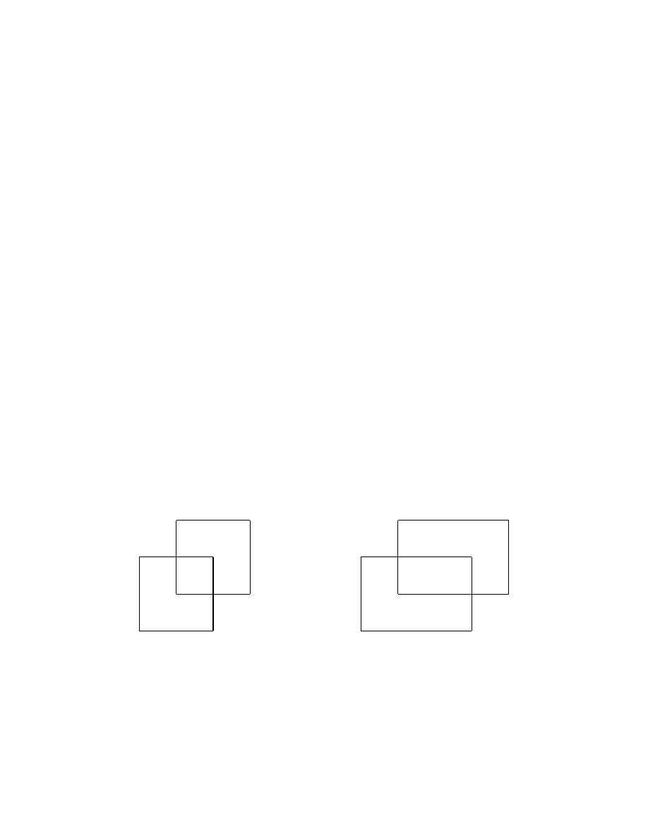
34
THOMAS WARD
example, because that is mixing on 2 sets but not on 3 sets, which is
witnessed by a non-mixing shape.
The result that may be proved using the methods of [
] proves
Conjecture
for some more cases.
Theorem 4.10. If p = hf i is a principal R
(p)
d
-module, and the support
of f comprises the vertices of a tight polyhedra, then Conjecture
holds for α
R
(p)
d
/p
.
In the remainder of this section we will explain what this means and
how it comes about by proving it for d = 2.
The type of polyhedra we are interested in are convex hulls of finite
sets of points in Z
d
.
Definition 4.11. A parallel redrawing of a polyhedron P is another
polyhedron P
0
with the property that each edge e of P is parallel to a
single edge of P
0
. A polyhedron is tight if any parallel redrawing must
be homothetic to the original polyhedron.
The terminology is taken from the slightly different setting of [
and [
Example 4.12. To make sense of Definition
, consider the follow-
ing examples.
(1) For d = 2 there is only one tight shape, and that is the triangle.
(2) For d = 3 there are many tight polyhedra. Roughly speaking,
a polyhedron with many triangular faces will be tight.
Figure 9. A parallel redrawing of the cube
(3) Of the platonic solids, the tetrahedron, octahedron and icosa-
hedron are tight, while the cube and dodecahedron are loose.
(4) All the geodesates are tight. This gives many easy examples of
very complex tight polyhedra.

VALUATIONS AND HYPERBOLICITY IN DYNAMICS
35
J
J
J
J
J
J
J
J
J
J
J
J
Figure 10. The tetrahedron is tight
Let
M(α
R
(p)
d
/hf i
) denote the order of mixing – the largest value of
r for which (
) – of α
R
(p)
d
/hf i
, where f is an irreducible
polynomial in F
p
[u
±1
1
, u
±2
2
]. Finding
M(α
R
(p)
d
/hf i
) is difficult (see [
Sect. 28]) even for this special class of systems. Let S(f ) denote the
support of f , and
N(f) the convex hull of S(f).
Theorem 4.13. Assume that
N(f) is an R-gon and f is irreducible.
Then
R − 1 ≤
M(α
R
(p)
d
/hf i
) < |S(f )|.
Theorem 4.14. Conjecture
holds when r = 3.
The method of proof of Theorem
is to show that an arbitrary
non-mixing sequence for α
R
2
/p
must asymptotically reflect part of the
structure of
N(f) (the slopes of the faces). Proving Conjecture
would involve showing that the exact structure of
N(f) appears, and
the reason Theorem
holds is that a triangle is the only tight polyhe-
dron in 2 dimensions. Thus Theorem
is a special case of Theorem
The key step in the proof is to construct valuations that reflect the
geometry of
N(f). To clarify this, an example is described in detail.
Example 4.15. Let f (u
1
, u
2
) = u
2
+ u
1
+ u
3
1
u
2
, and view f as an ele-
ment of F
p
(u
2
)[u
1
]. Choose a norm | · | on F
p
(u
2
) with |u
2
| =
1
p
. This
norm extends in two ways to the field K = F
p
(u
2
)[u
1
]/hf i, determined
by the Newton polygon of f viewed as a polynomial for u
1
with coef-
ficients in F
p
(u
2
). The four points that define the Newton polygon are
(0, − log
p
|u
2
|), (1, − log
p
|1|), (2, ∞) and (3, − log
p
|u
2
|). From Figure
it follows that the two extended norms | · |
1
, | · |
2
have |u
1
|
1
=
1
p
(from the line segment with slope −1) and |u
1
|
2
=
√
p (from the line
segment with slope 1/2).
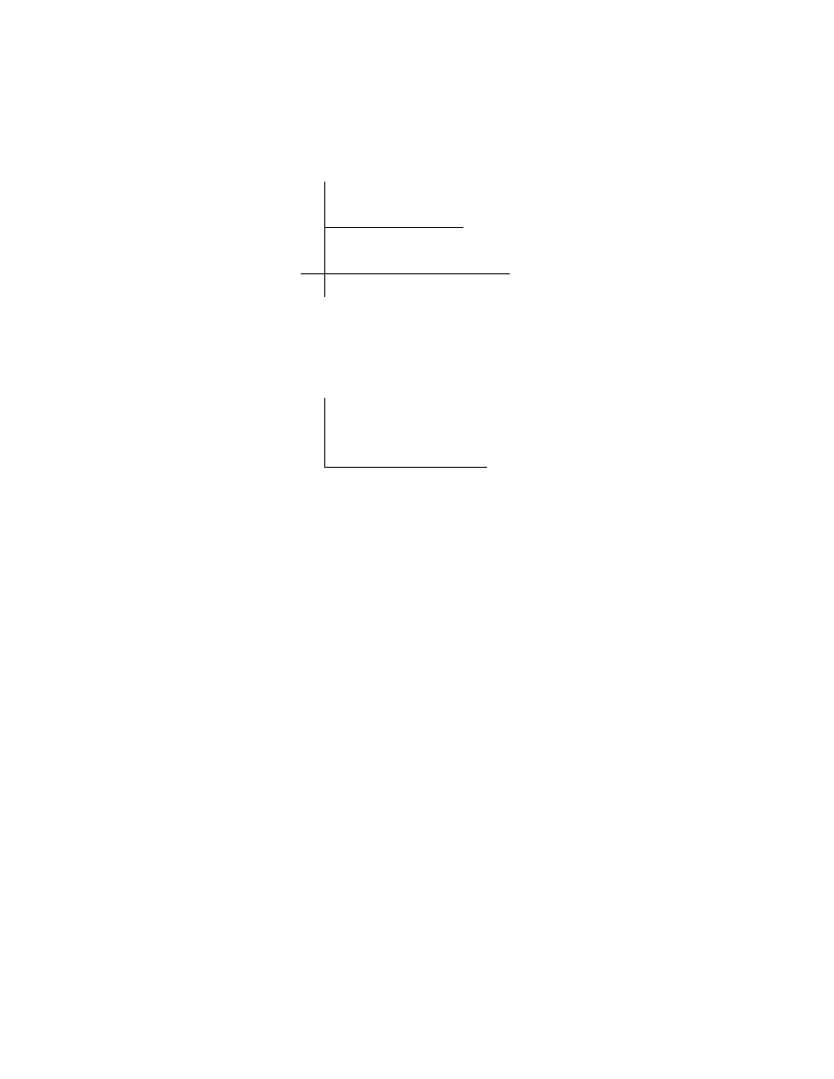
36
THOMAS WARD
@
@
@
@
F
1
F
2
F
3
u
1
u
2
u
3
1
u
2
Figure 11. The faces of N(u
2
+ u
1
+ u
3
1
u
2
)
@
@
@
@
1
1
2
3
r
r
r
Figure 12. The Newton polygon of f ∈ F
p
(u
2
)[u
1
]
Thus the vector
log
p
|u
1
|
1
log
p
|u
2
|
1
=
−1
−1
is normal to the face F
1
and
points out from
N(f). The same expression using |·|
2
gives an outward
normal to the face F
2
.
Finally, if the initial norm on F
p
(u
2
) is chosen with |u
2
| = p, then
the corresponding Newton polygon shows only one extension, and the
resulting norm gives an outward normal to the face F
3
.
Proposition 4.16. Assume that A
(j)
= (n
(j)
1
, n
(j)
2
, . . . , n
(j)
r
) is a se-
quence with the property that
(4.9)
m
1
u
n
(j)
1
+ m
2
u
n
(j)
2
+ · · · + m
r
u
n
(j)
r
= 0
for all j, where m
1
, . . . , m
r
∈ R/p\{0}. Write
N(A
(j)
) for the convex
hull of A
(j)
. Then there is a constant K > 0 such that for each face F
of
N(f) there is a face of N(A
(j)
) spanned (without loss of generality)
by n
(j)
1
, n
(j)
2
, and there is a vector m
(j)
with the property that the line
through n
(j)
1
, m
(j)
is parallel to F and km
(j)
− n
(j)
1
k ≤ K.
Proof. Pick a face F of
N(f). Using the irreducibility of f, construct
as in Example
a norm | · | on R
2
/hf i so that
log
p
|u
1
|
log
p
|u
2
|
is an
outward normal to
N(f) through F .

VALUATIONS AND HYPERBOLICITY IN DYNAMICS
37
Choose K so that K ≥ 2 max
i=1,...,r
{
log
p
|m
i
|
}.
Find an F -exposed vertex p
j
= n
(j)
t
in A
(j)
, let ` be the line through
p
j
parallel to F , and assume that no other point in A
(j)
is within
distance K of `. Then for n
(j)
i
6= p
j
, log
p
|u
n
(j)
i
m
i
| < log
p
|u
p
j
m
t
|,
which contradicts (
). It follows that there is another vertex of A
(j)
within the strip as required.
Proof. (of Theorem
) First recall that S(f ) is automatically a non-
mixing shape for α
R
(p)
d
/hf i
by the method of proof of Theorem
, so
M(α
R
(p)
d
/hf i
) < |S(f )|. On the other hand, each of the R faces of
N(f)
must asymptotically appear in
N(A
(j)
) for a non-mixing sequence (A
(j)
)
by Proposition
. It follows that R − 1 ≤
M(α
R
2
/p
).
Proof. (of Theorem
) If
N(f) lies on a line, then α
R
(p)
d
/hf i
cannot
be mixing. If
N(f) is an R-gon with R > 3 then Theorem
shows
that
M(α
R
(p)
d
/hf i
) ≥ 3. So assume that
N(f) is a triangle, that α
R
(p)
d
/hf i
is not mixing on 3 sets, and that all triangles are mixing shapes for
α
R
(p)
d
/hf i
. This means that there are non-zero polynomials a, b, c with
au
n
(j)
1
+ bu
n
(j)
2
+ cu
n
(j)
r
= 0
for all j. By Proposition
each of n
(j)
1
, n
(j)
2
, n
(j)
3
lie within a bounded
distance of the vertices of some dilate of
N(f). Multiplying a, b, c by
monomials chosen to shift the vertices a bounded distance onto the
vertices of an integer dilate of S(f ), produces an equation
a
0
u
m
(j)
1
+ b
0
u
m
(j)
2
+ c
0
u
m
(j)
r
= 0
that witnesses a non-mixing shape of order 3. This contradicts the
assumption.
Example 4.17. Theorem
shows that if f is an irreducible poly-
nomial for which the support S(f ) coincides with the extreme points of
the Newton polygon
N(f), then M(α
R
(p)
d
/hf i
) = |S(f )| − 1. In order to
produce an example with prescribed order of mixing
M(α
R
(p)
d
/hf i
) = k,
it is therefore sufficient to exhibit such an irreducible polynomial with
|S(f )| = k + 1. This may be done using Eisenstein’s irreducibility
criterion (see [
] for a general valuation-theoretic treatment of the
Eisenstein criterion). Two simple examples will illustrate the method;
it is clear from these how to build an example for any order of mixing.
(1) To find an example with order of mixing 3, consider f (u
1
, u
2
) =
u
2
1
+ u
1
u
2
2
+ u
3
2
+ u
2
∈ F[u
2
][u
1
]; the prime u
2
∈ F[u
2
] divides the
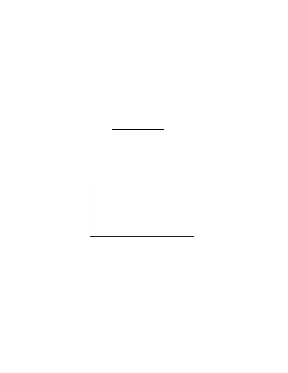
38
THOMAS WARD
coefficients u
2
2
and u
3
2
+ u
2
but u
2
2
does not divide the coefficient
u
3
2
+ u
2
. The support of the polynomial is shown in Figure
H
H
H
H
H
H
H
@
@
@
@
A
A
A
A
A
A
A
u
2
1
u
2
u
3
2
u
1
u
2
2
r
r
r
r
Figure 13. The support of a polynomial giving 3-fold mixing
(2) To find an example with order of mixing 4, let f (u
1
, u
2
) =
u
6
1
+u
5
1
u
2
+u
3
1
u
2
2
+u
2
+u
3
2
. As before, this is seen to be irreducible
by viewing it as a polynomial in u
1
with coefficients in F[u
2
].
The support of the polynomial is shown in Figure
hhh
hhh
hhh
hhh
hhh
hhh
hh
h
P
P
P
P
P
P
P
P
P
P
P
H
H
H
H
H
H
H
@
@
@
@
u
6
1
r
u
2
r
u
3
2
r
r
u
3
1
u
2
2
r
u
5
1
u
2
Figure 14. The support of a polynomial giving 4-fold mixing
Notice that in these examples we are choosing the shape of the support
freely; it is also possible to find examples for which any prescribed shape
is the minimal non-mixing shape by [
], though not in a constructive
fashion.
Example 4.18. Theorem
shows that the system corresponding
to the ideal p = h2, 1 + u
1
+ u
2
+ u
2
2
i is 3-mixing, answering a question
in [
, p. 283].
Example 4.19. In the previous example, we used the fact from [
that no shape with cardinality 3 is non-mixing. An alternative method
to show this is to use a result of Voloch on solutions to ax + by = 1 in

VALUATIONS AND HYPERBOLICITY IN DYNAMICS
39
functions fields. Consider again p = h2, 1 + u
1
+ u
2
+ u
2
2
i; then Theorem
says that
2 ≤
M(α
R
2
/p
) < 4,
and we wish to show that
M(α
R
2
/p
) = 3. To see this, assume that
n
(j)
1
, n
(j)
2
, n
(j)
3
= 0
is a non-mixing sequence for α
R
2
/p
with n
(j)
s
− n
(j)
t
→ ∞ as j → ∞ for
s 6= t. Then there are elements m
1
, m
2
, m
3
of R
2
/p, not all zero, with
(4.10)
m
1
u
n
(j)
1
+ m
2
u
n
(j)
2
= −m
3
for infinitely many j. The field of fractions of R
2
/p may be identified
with F
2
(t) by the map u
1
7→ t, u
2
7→ 1 + t + t
2
, and in this field (
becomes
(4.11)
ax + by = 1
with infinitely many solutions for x, y in the finitely generated multi-
plicative subgroup G = hht, 1 + t + t
2
ii of F
2
(t)
∗
. By [
], it follows that
) is a G-trivial equation: there is an n ≥ 1 for which a
n
, b
n
∈ G.
Since G is generated by irreducible polynomials, this can only be true
if a, b ∈ G. So there is an infinite family of equations
(4.12)
u
m
(j)
1
+ u
m
(j)
2
= 1
with m
(j)
1
, m
(j)
2
, and m
(j)
1
− m
(j)
2
→ ∞ as j → ∞. By considering the
shape of
N(1+u
1
+u
2
1
+u
2
), this shows that the polynomial in (
) has
the same shape as
N(1 + u
1
+ u
2
1
+ u
2
), so (without loss of generality),
m
(j)
1
= (0, m(j)) and m
(j)
2
= (2m(j), 0) for some m(j) → ∞. Thus the
equation reduces to
(4.13)
(1 + t + t
2
)
m(j)
= 1 + t
2m(j)
.
Write m(j) = 2
e
`, ` odd, for some e ≥ 0. Then the left-hand side of
) is
(1 + t + t
2
)
2
e
`
= (1 + t + O(t
2
))
2
e
= 1 + t
2
e
+ O(t
2
)
2
e
= 1 + t
2
e+1
`
,
which is impossible. It follows that
M(α
R
2
/p
) = 3.

40
THOMAS WARD
4.4. Typical actions. The analogue of Section
is even less acces-
sible for commuting automorphisms. The entropy has been computed
in terms of the prime ideals associated to the module – see [
, Th. 4.4]
– and is built up from the cyclic case.
Theorem 4.20. The topological entropy of the Z
d
-action α
R
d
/p
is 0 if
p
is non-principal, and is given by
h(α
R
d
/p
) = m(f ) =
Z
1
0
. . .
Z
1
0
log |f (e
2πis
1
, . . . , e
2πis
d
)|ds
1
. . . ds
d
if p = hf i.
It turns out that Lehmer’s Problem
is not changed by passing
to more variables: 0 is a cluster point of {m(f ) | f ∈ Z[x]} if and only
if 0 is a cluster point of {m(f ) | f ∈ R
d
} for some d ≥ 1. This is a
consequence of a non-trivial approximation result due to Lawton [
(see [
] for a simple treatment). It follows that it is not known what
the possible entropies of algebraic Z
d
-actions are.
Beyond that, the algebra of higher-rank S-integer systems is quite
subtle, and there are real difficulties associated with formulating the
analogue of S-integer dynamical systems in higher rank. For some
results see [
5. Subdynamics
As we have seen, the problem of understanding the dynamics of alge-
braic Z
d
-actions can always be reduced to statements in commutative
algebra, and for these valuations are a powerful tool. The last dynam-
ical property we will discuss is the geometric notion of subdynamics:
for a given Z
d
-action, what properties do lower-rank subactions have?
The material here is taken from the papers [
Let β be a Z
d
-action by homeomorphisms of a compact metric space
(X, ρ). For a subset F of R
d
define a new (pseudo-)metric by
ρ
F
β
(x, y) = sup{ρ β
n
(x), β
n
(y)
: n ∈ F ∩ Z
d
},
and if F ∩ Z
d
= ∅ define ρ
F
β
(x, y) = 0.
Definition 5.1. The Z
d
-action β on (X, ρ) is said to be expansive if
there is a δ > 0 with the property that
(5.1)
ρ
R
d
β
(x, y) ≤ δ ⇒ x = y.
Any δ > 0 satisfying (
) is called an expansive constant for β.

VALUATIONS AND HYPERBOLICITY IN DYNAMICS
41
For t > 0, let
F
t
= {x ∈ R
d
: dist(x, F ) ≤ t},
where dist denotes the usual Euclidean distance. Thus F
t
is the result
of thickening F by t. This device of considering thickened subsets
comes from [
] and is an implicit way of passing from the countable
collection of rational subspaces of Q
d
to the compact Grassmanian. An
alternative way to compactify the space of directions is to replace the
original Z
d
-action with a R
d
-flow on a suspension – see [
Definition 5.2. A subset F ⊂ R
d
is expansive for β if there are ε > 0
and t > 0 such that
ρ
F
t
β
(x, y) ≤ ε ⇒ x = y.
Every subset of a nonexpansive set for β is nonexpansive for β. Every
translate of an expansive set is expansive by [
, p. 57]. In Definition
ε can be fixed for β [
, Lemma 2.3].
Let G
k
= G
d,k
denote the Grassmann manifold of k-dimensional sub-
spaces (or k-planes) of R
d
; G
k
is a compact manifold of dimension
k(d − k) whose topology is given by declaring two subspaces to be close
if their intersections with the unit sphere are close in the Hausdorff
metric.
Definition 5.3. For a Z
d
-action β define
E
k
(β) = {V ∈ G
k
: V is expansive for β},
N
k
(β) = {V ∈ G
k
: V is nonexpansive for β}.
An expansive component of k-planes for β is a connected component
of E
k
(β).
Example 5.4. [ledrappier’s example] Take d = 2,
X = {x ∈ (Z/2Z)
Z
2
: x
i,j
+ x
i+1,j
+ x
i,j+1
≡ 0 (mod 2) for all i, j},
and let β be the Z
2
-action generated by the horizontal and vertical
shifts. If L is a line that is not parallel to one of the sides of the unit
simplex in R
2
and t ≥ 2, then for each x ∈ X the coordinates of x
within L
t
determine all of x, so that L ∈ E
1
(β). On the other hand,
the three lines parallel to the sides of the simplex do not have this
property, and they comprise N
1
(β) (see [
, Example 2.7] for details).
Coding arguments [
, Lemma 3.4] show that each E
k
(β) is an open
subset of G
k
, so that each N
k
(β) is compact. Hence expansive compo-
nents of k-planes for β are open subsets of G
k
. If W is nonexpansive
for β and V is a subspace of W , then V is also nonexpansive for β.

42
THOMAS WARD
A basic result [
, Theorem 3.6] is a sort of converse to this: If V is
a nonexpansive subspace for β of dimension ≤ d − 2, then there is a
nonexpansive subspace for β containing V of one higher dimension. If
X is infinite, then the zero subspace is nonexpansive, and hence each
N
k
(β) 6= ∅ for 1 ≤ k ≤ d − 1. Hence N
k
(β) consists of exactly all
k-dimensional subspaces of the subspaces in N
d−1
(β). Thus N
d−1
(β)
determines the entire expansive subdynamics of β.
In order to treat algebraic Z
d
-actions, it is convenient to shift our
viewpoint slightly and use half-spaces in R
d
rather than (d − 1)-planes.
Let S
d−1
= {v ∈ R
d
: kvk = 1} be the unit (d−1)-sphere. For v ∈ S
d−1
define H
v
= {x ∈ R
d
: x · v ≤ 0} to be the half-space with outward
unit normal v. Let H
d
be the set of half-spaces in R
d
, which we identify
with S
d−1
via the parameterization v ↔ H
v
. For H ∈ H
d
we denote
its outward unit normal vector by v
H
.
Expansiveness along a half-space H is defined using Definition
with F = H. Observe that thickening H
v
by t > 0 results merely
in the translation H
v
+ tv of H
v
. Hence there is no need to thicken
half-spaces in the definition, and a Z
d
-action β is therefore expansive
along H if and only if there is an ε > 0 such that ρ
H
β
(x, y) ≤ ε implies
that x = y.
Definition 5.5. For a Z
d
-action β define
E(β) = {H ∈ H
d
: H is expansive for β},
N(β) = {H ∈ H
d
: H is nonexpansive for β}.
An expansive component of half-spaces for β is a connected component
of E(β).
Remark 5.6. A coding argument analogous to [
, Lemma 3.4] shows
that E(β) is an open set and so N(β) is a compact set.
The following lemma shows that a (d − 1)-plane is nonexpansive
for β if and only if at least one of the two bounding half-spaces is also
nonexpansive for β. Thus if we define π : H
d
→ G
d−1
by π(H) = ∂H,
then π(N(β)) = N
d−1
(β). This shows that the half-space behavior N(β)
determines the expansive subdynamics of β.
The following key definition is taken from [
, Definition 3.1].
Definition 5.7. Let β be an expansive Z
d
-action with expansive con-
stant δ. For subsets E, F of R
d
we say that E codes F provided that,
for every x ∈ R
d
, if ρ
E+x
β
(x, y) ≤ δ then ρ
F +x
β
(x, y) ≤ δ.
Lemma 5.8. Let β be a Z
d
-action and V ∈ G
d−1
. Then V ∈ N
d−1
(β)
if and only if there is an H ∈ N(β) with ∂H = V .

VALUATIONS AND HYPERBOLICITY IN DYNAMICS
43
Proof. If H ∈ N(β), then V = ∂H ⊂ H is also nonexpansive.
Conversely, let V ∈ G
d−1
and H = H
v
, H
0
= H
−v
be the two half-
spaces with boundary V . Suppose that both H and H
0
are expansive
for β. We prove that V is also expansive for β, which will complete the
proof.
Since β has an expansive half-space, it is an expansive action. Let
δ > 0 be an expansive constant for β. Let B(r) denote the ball of
radius r in R
d
, and [0, v] be the line segment joining 0 to v. A “finite”
version of the expansiveness of H, entirely analogous to [
, Lemma 3.2],
is that there is an r > 0 such that H ∩B(r) codes [0, v]. Similarly, there
is an s > 0 such that H
0
∩ B(s) codes [0, −v]. Hence if t = max{r, s},
then V
t
codes V
t+1
, which by the same argument codes V
t+2
, and so
on. Thus V
t
codes R
d
, which means that V is expansive.
As a starting point, Schmidt [
] gave the following characterization
of expansiveness for α
M
. For an ideal p ⊂ R
d
, let
V(p) =
z = (z
1
, . . . , z
d
) ∈ (C
×
)
d
: f (z
1
, . . . , z
d
) = 0 for all f ∈ p
.
Let S
d
= {(z
1
, . . . , z
d
) ∈ C
d
: |z
1
| = · · · = |z
d
| = 1} be the multiplica-
tive d-torus.
Theorem 5.9. The Z
d
-action α
M
is expansive if and only if both
(1) M is a Noetherian R
d
-module, and
(2) for each prime ideal p ⊂ R
d
associated to M , V (p) ∩ S
d
= ∅.
The first condition – algebraic in nature – is necessary for the follow-
ing reason. If M is not Noetherian, then there is an infinite ascending
chain of submodules {0} ⊂ M
1
⊂ M
2
⊂ . . . inside M ; their annihila-
tors form an infinite descending chain of closed α
M
-invariant subgroups
{0}
⊥
= X
M
⊃ M
⊥
1
⊃ M
⊥
2
⊃ . . . with
T
j≥1
M
⊥
j
= {0}, showing that
α
M
is not expansive. The second condition – which is geometric – is
necessary because from a point in V (p)∩S
d
a point may be constructed
whose orbit under the action of α
M
stays close to 0.
The main result in [
] is a directional version of this theorem. There
are several steps involved in this, and the two different requirements
for expansiveness each have their own analogues. For H ∈ H
d
, define
the ring R
H
= Z[u
n
: n ∈ H ∩ Z
d
], which is a subring of R
d
. In general
R
H
is not Noetherian; indeed, R
H
is Noetherian exactly when v
H
is
a rational direction in the sense that Rv
H
∩ Z
d
6= {0}, so that R
H
is
Noetherian for only countably many H.
Theorem 5.10. Let M be a Noetherian R
d
-module, α
M
be the cor-
responding algebraic Z
d
-action, and H ∈ H
d
. Then the following are
equivalent.

44
THOMAS WARD
(1) α
M
is expansive along H.
(2) α
R
d
/p
is expansive along H for every prime ideal p associated
to M .
(3) R
d
/p is R
H
-Noetherian and [0, ∞)v
H
∩ log |V(p)| = ∅ for every
p
∈ asc(M ).
In order to work with this result, it is important to give a more
computable version of the R
H
-Noetherian property. This is discussed
in detail in [
] we take the following theorem.
Theorem 5.11. Let M be a Noetherian R
d
-module, H ∈ H
d
, and
k ∈ Z
d
r H.
Then M is R
H
-Noetherian if and only if there is a
polynomial of the form u
k
− f (u) with f (u) ∈ R
H
that annihilates M .
It follows that there is an algorithm that describes the set of those H
for which a given module M is R
H
-Noetherian.
The last part of this theorem relates to a slightly different kind of
problem than those we have mentioned. That is, given a presentation
of a module, how does one set about actually computing some of the
dynamical properties of the associated system? In particular, for which
properties are complex syzygy computations required? See [
Sect. 6] for some discussion of this.
5.1. Examples. Using the correspondence H
d
↔ S
d−1
given by H ↔
v
H
, subsets of H
d
may be identified with the corresponding subsets of
S
d−1
. Using this convention, for an ideal a ∈ R
d
define
N
n
(α
R
d
/a
) = {v ∈ S
d−1
: R
d
/a is not R
H
v
-Noetherian},
N
v
(α
R
d
/a
) = {v ∈ S
d−1
: [0, ∞)v ∩ log |V(a)| 6= ∅}.
Observe that N
v
(α
R
d
/a
) is the radial projection of log |V(a)| to S
d−1
.
By Theorem
N(α
R
d
/a
) = N
n
(α
R
d
/a
) ∪ N
v
(α
R
d
/a
).
In the case of a principal ideal hf i in R
d
we abbreviate V(hf i) to V(f ).
Example 5.12. Consider Example
again. As we saw, this has
a surprisingly mixing property, despite having zero entropy.
Here
M = R
2
/hu
1
− 2, u
2
− 3i; the corresponding dynamical system α is
the invertible extension of the semi-group action generated by x 7→ 2x
and x 7→ 3x mod 1 on the additive circle. Write p = hu
1
− 2, u
2
−
3i. To use Theorem
, notice that V (p) = {(2, 3)}, so the vari-
ety condition [0, ∞)v
H
∩ log |V(p)| = ∅ will fail only in the direction
v
H
= (log 2, log 3). The module M is R
H
-Noetherian except when
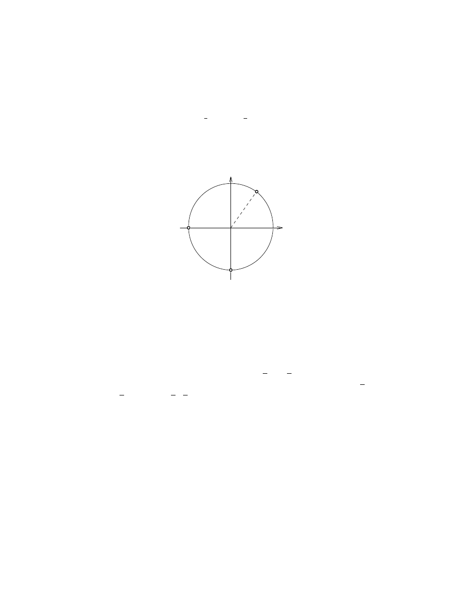
VALUATIONS AND HYPERBOLICITY IN DYNAMICS
45
v
H
= (0, −1) or (−1, 0). A sample of these arguments is the following:
if v
H
= (−1, 0), then R
H
is the ring R
H
= Z[u
1
, u
±1
2
], and so
R
2
/p ⊃ · · · ⊃
1
4
R
H
/p ⊃
1
2
R
H
/p ⊃ R
H
/p ⊃
is an infinite ascending chain of R
H
-submodules, showing this direction
to be non-Noetherian. The non-expansive set is shown in Figure
using the convention above associating subsets of the Grassmanian to
subsets of the (d − 1)-sphere.
Figure 15. Non-expansive directions for ×2, ×3.
Ledrappier’s example will have a similar picture, and these are rep-
resentative of the possible type of phenomena in Z
2
-actions. For Z
3
-
actions, there are many new possible phenomena.
Example 5.13. The following example is taken from Miles’ thesis [
Example 4.3.7], which constructs the systems in a different way. If X
is the dual of the ring of integers in Q(
√
2 +
√
5), with a Z
3
-action
α induced by the automorphisms dual to multiplication by 1 +
√
2,
2 +
√
5, and 3 +
√
2
√
5. Here there are four non-expansive planes in
general position, leaving seven expansive cones shown in Figure
Understanding the next example exhibits several new phenomena
that arise in Z
d
-actions for d ≥ 3. First, there may be no expansive
lines at all. Second, a set of expansive directions may have curved sides.
Finally, the set of non-expansive behaviour may have interior. It is not
possible to draw the corresponding set of non-expansive planes, so the
figure just shows the set of non-expansive vectors on the 2-sphere that
are outward normals to non-expansive half-planes.
Example 5.14. Let d = 3 and p = h1 + u
1
+ u
2
, u
3
− 2i. This is a
prime ideal (see [
] for the details of this argument). Since V(p) =
{(z, −z − 1, 2) : z ∈ C}, log |V(p)| lies in a plane at height log 2 above
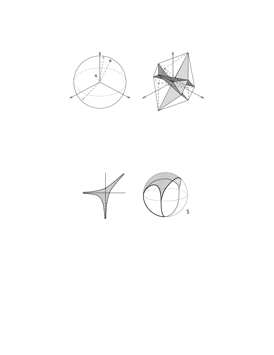
46
THOMAS WARD
(b)
(a)
Figure 16. Non-expansive directions on the sphere and
the corresponding planes.
the origin, and in this plane it has the shape shown in Figure
(a),
where the boundary curves are parameterized by (log r, log |r ± 1|) for
0 < r < ∞. When projected onto S
2
, the set in the upper hemisphere
shown in Figure
(b) results, with three cusps on the equator.
2
(a)
(b)
Figure 17. A nonexpansive set with interior.
Using Theorem
, the polynomial u
3
− 2 ∈ p witnesses that the
open upper hemisphere in S
2
is disjoint from N
n
(α
R
3
/p
). Moreover,
1 + u
1
+ u
2
∈ p shows that no points in the lower hemisphere are in
N
n
(α
R
3
/p
) either, with the possible exceptions of those on the three
quarter meridians shown in Figure
(b). We will show that each of
these quarter meridians is contained in N
n
(α
R
3
/p
), so that they, com-
bined with N
v
(α
R
3
/p
) in the upper hemisphere, comprise all of N(α
R
3
/p
).
We will treat the meridian from (0, −1, 0) to (0, 0, −1), the other two
being similar. It is enough to show that unit vectors in the directions
(0, −a, −b) are non-Noetherian, where a and b are positive integers (an
argument in [
] shows that N
n
(α
R
3
/p
) is itself closed). Let H ∈ H
3

VALUATIONS AND HYPERBOLICITY IN DYNAMICS
47
be {x ∈ R
3
: x · (0, a, b) ≥ 0}. The isomorphism φ : f 7→ f (t, −t −
1, 2), φ : R
3
/p → Z[t, 1/2t(t + 1)] sends the subring R
H
to Z[t
±1
, (−t −
1)
m
2
n
: am + bn ≥ 0].
Then R
3
/p is Noetherian over R
H
if and
only if Z[t, 1/2t(t + 1)] is finitely generated over Z[t
±1
, (−t − 1)
m
2
n
:
am + bn ≥ 0]. Using the characterisation from Theorem
again,
this is equivalent to whether we can write 1 as a combination, using
coefficients in Z[t
±1
], of expressions of the form (−t − 1)
m
2
n
, where
am + bn > 0. Suppose this to be the case, so that
(5.2)
1 =
X
(m,n)∈F
f
mn
(t)(−t − 1)
m
2
n
,
where f
mn
(t) ∈ Z[t
±1
] and F is a finite set of (m, n) ∈ Z
2
for which
am + bn > 0. Let | · |
2
denote the extension of the 2-adic norm on Q
to Q(2
1/b
). Substitute t = 2
a/b
− 1 in (
). Since |2
a/b
− 1|
2
= 1, it
follows that |f
mn
(2
a/b
− 1)|
2
≤ 1. Hence
1 = |1|
2
=
X
(m,n)∈F
f
mn
(2
a/b
− 1)(−2
a/b
)
m
2
n
2
≤ max
(m,n)∈F
f
mn
(2
a/b
− 1)
2
−2
a/b
m
2
2
n
2
≤ max
(m,n)∈F
2
−(am+bn)/b
< 1.
This contradiction shows that (
) is impossible, so that each rational
direction (0, −a, −b) is non-Noetherian.
5.2. Adelic amoebas. In Theorem
two entirely different kinds
of reasons for non-expansiveness were presented: the module may fail
to be Noetherian along the half-space H, or it may fail the variety
condition. It turns out that this distinction in kind is not really neces-
sary, and a valuation-theoretic approach gives a cleaner picture. This
section is taken from Miles’s thesis [
] and recent work of Einsiedler,
Lind and Ward [
Example 5.15. To understand this, start with the very simple Ex-
ample
. There were three points in N, one coming from N
v
as a
result of the point (2, 3) in the variety, and two coming from N
n
cor-
responding to the two non-Noetherian directions. Now consider the
logarithmic image of the same variety over Q
2
: the point (2, 3) ∈ Q
2
2
has (log |2|
2
log |3|
2
) = (− log 2, 0), giving the direction (−1, 0). Simi-
larly, the logarithmic image of the variety over Q
3
gives the direction
(0, −1). Of course it is not really legitimate to select the primes 2
and 3 after we knew the answer: however, for any other prime p, the
logarithmic image of the variety over Q
p
comprises the point (0, 0),

48
THOMAS WARD
which does not project to anything more on the circle. So the union
of the projections of the p-adic amoebas over all p ≤ ∞ describes the
non-expansive set.
The same thing holds in general, though it is a quite subtle and
lengthy proof. With Theorem
taking care of the p = ∞ part,
it amounts to proving a statement purely in commutative algebra.
Namely: the directional Noetherian property is governed by the p-adic
amoebas. A key step is to relate Theorem
, an integrality condition,
to the existence of a valuation that witnesses non-integrality.
Definition 5.16. For a prime ideal p ∈ R
d
, define the usual amoeba
to be
Am(p) = Am
∞
(p) = {(log |z
1
|, . . . , log |z
d
| | z ∈ V
C
(p)},
where V
C
denotes the variety over C
ast
. Similarly, for each prime p
denote the p-adic amoeba by
Am
p
(p) = {(log |z
1
|
p
, . . . , log |z
d
|
p
| z ∈ V
C
p
(p)}.
Finally define the adelic amoeba to be Am
A
(p) =
S
p≤∞
Am
p
(p).
Theorem 5.17. The non-expansive set N(α
R
d
/p
) is equal to the pro-
jection of Am
A
(p) onto S
d−1
.
Example 5.18. Consider Example
again. Here d = 3 and p =
h1 + u
1
+ u
2
, u
3
− 2i. The usual amoeba of p is that subset of R
3
defined
by
Am
∞
(p) = {(a, b, log 2) | (a, b) ∈ V
C
(h1 + x + yi)},
which looks like a copy of Figure
(a) parallel to the (x, y)-plane at
the level z = log 2.
To compute the p-adic amoebas, first let k be any ultrametric field
with valuation | · | and consider the (x, y) part. Then
(x, y) ∈ V
k
(h1 + x + yi) ⇒ |x| = |1 + y|,
so
log |y| < 0 ⇒ |y| < 1 ⇒ |x| = 1
by the ultrametric inequality. This means the negative y-axis is part of
the amoeba. By symmetry, the negative x-axis is also in the amoeba.
On the other hand,
log |y| > 0 ⇒ |y| > 1 ⇒ |x| = |y|
by the ultrametric inequality again.
Now let p = 2. By the argument above, the 2-adic amoeba is the
shape shown in Figure
since it lies at level z = log |2|
2
= − log 2.
VALUATIONS AND HYPERBOLICITY IN DYNAMICS
49
-
6
3
x
z
y
− log 2
Figure 18. The 2-adic amoeba of h1 + u
1
+ u
2
, u
3
− 2i
For primes p 6= 2, the amoeba has the same shape in the (x, y)-plane,
but at the level z = log |2|
p6=2
= 0, as shown in Figure
. Projecting
-
6
3
x
z
y
Figure 19. The 2-adic amoeba of h1 + u
1
+ u
2
, u
3
− 2i
these shapes onto the unit sphere gives the shape in Figure
The p-adic amoebas also arise in the Biere-Strebel invariant in group
theory – see [
] for more details.
6. Some directions for future research
6.1. Typical group automorphisms. As we saw in Section
, the
complete picture of how many periodic points a ‘typical’ group auto-
morphism has is still unknown.
6.2. Periodic points. How many periodic points can a compact group
endomorphism have? There are some surprising examples here: in [
a compact group automorphism T is constructed with the property that

50
THOMAS WARD
Per
n
(T ) is the denominator of B
2n
(the Bernoulli numbers). Specifi-
cally, if (u
n
)
n≥1
is a sequence of positive integers with the properties
X
d|n
µ(n/d)u
d
≡ 0 mod n for all n ≥ 1 (Congruence),
X
d|n
µ(n/d)u
d
≥ 0 for all n ≥ 1 (Positivity), and
m|n ⇒ u
m
|u
n
for all n ≥ 1 (Divisibility)
is there a compact group automorphism T with u
n
= Per
n
(T ) for all
n ≥ 1? For more on this, see [
6.3. Mixing problem. Is there a dynamical proof of Theorem
Even a dynamical proof that Example
is mixing of all orders seems
difficult.
Is Conjecture
true? The results known suggest that there are
two obstacles even for the case of principal ideals. First, the Newton
polygon may be loose, opening up the possibility of a non-mixing se-
quence that approximates the wrong shape. Secondly, the polynomial
itself may have non-zero coefficients deep inside its support.
6.4. Entropy. The outstanding problem here is Lehmer’s problem of
course.
6.5. Entropy and Deligne periods. A very interesting problem has
been raised by Deninger in the course of his work on Mahler measures.
In [
] he showed – roughly speaking – that m(f ) is the Deligne period
of a certain mixed motive associated in a canonical way to f . Using a p-
adic analogue of Deligne cohomology gives an analogous p-adic valued
Mahler measure, m
p
, described in [
]. The question raised there is
whether there is a p-adic valued notion of entropy that gives entropy
m
p
(f ) to the dynamical system associated to f . A specific form of
this general question is the following. Define log
p
: C
∗
p
→ C
p
to be
the branch of the p-adic logarithm with log
p
(p) = 0, and consider
the map T
λ
: x 7→ λx on (say) Q
p
. Is there a meaningful entropy-
like invariant h
p
(invariant under topological conjugacy, for example)
with h
p
(T
λ
) = log
p
λ? For more background on the theory behind
this question, see [
, Sect. 1.8]; for background on these questions and
mixed motives, see [

VALUATIONS AND HYPERBOLICITY IN DYNAMICS
51
References
[1] Nobuo Aoki and Haruo Totoki, Ergodic automorphisms of T
∞
are Bernoulli
transformations, Publ. Res. Inst. Math. Sci. 10 (1974/75), 535–544. MR 52
#701
[2] Amnon Besser and Christopher Deninger, p-adic Mahler measures, J. Reine
Angew. Math. 517 (1999), 19–50. MR 2001d:11070
[3] Robert Bieri, Walter D. Neumann, and Ralph Strebel, A geometric invariant
of discrete groups, Invent. Math. 90 (1987), no. 3, 451–477. MR 89b:20108
[4] Robert Bieri and Ralph Strebel, A geometric invariant for modules over an
abelian group, J. Reine Angew. Math. 322 (1981), 170–189. MR 82f:20017
[5] Rufus Bowen, Entropy for group endomorphisms and homogeneous spaces,
Trans. Amer. Math. Soc. 153 (1971), 401–414. MR 43 #469
[6]
, On Axiom A diffeomorphisms, American Mathematical Society, Prov-
idence, R.I., 1978, Regional Conference Series in Mathematics, No. 35. MR 58
#2888
[7] David W. Boyd, Speculations concerning the range of Mahler’s measure,
Canad. Math. Bull. 24 (1981), no. 4, 453–469. MR 83h:12002
[8] Mike Boyle and Douglas Lind, Expansive subdynamics, Trans. Amer. Math.
Soc. 349 (1997), no. 1, 55–102. MR 97d:58115
[9] Robert Burton and Robin Pemantle, Local characteristics, entropy and limit
theorems for spanning trees and domino tilings via transfer-impedances, Ann.
Probab. 21 (1993), no. 3, 1329–1371. MR 94m:60019
[10] J. W. S. Cassels, Local fields, Cambridge University Press, Cambridge, 1986.
MR 87i:11172
[11] V. Chothi, G. Everest, and T. Ward, S-integer dynamical systems: periodic
points, J. Reine Angew. Math. 489 (1997), 99–132. MR 99b:11089
[12] Vijay Chothi, Periodic Points in S-integer Dynamical Systems, Ph.D. thesis,
Univ. of East Anglia, 1996.
[13] Jean-Pierre Conze, Points p´
eriodiques et entropie topologique, C. R. Acad. Sci.
Paris S´
er. A-B 267 (1968), A149–A152. MR 37 #6920
[14] Henry Crapo and Walter Whiteley, Spaces of stresses, projections and parallel
drawings for spherical polyhedra, Beitr¨
age Algebra Geom. 35 (1994), no. 2,
259–281. MR 96b:52036
[15] Christopher Deninger, L-functions of mixed motives, Motives (Seattle, WA,
1991), Amer. Math. Soc., Providence, RI, 1994, pp. 517–525. MR 95a:11058
[16]
, Deligne periods of mixed motives, K-theory and the entropy of certain
Z
n
-actions, J. Amer. Math. Soc. 10 (1997), no. 2, 259–281. MR 97k:11101
[17]
, On extensions of mixed motives, Collect. Math. 48 (1997), no. 1-2,
97–113, Journ´
ees Arithm´
etiques (Barcelona, 1995). MR 98f:11069
[18]
, Some analogies between number theory and dynamical systems on fo-
liated spaces, Proceedings of the International Congress of Mathematicians,
Vol. I (Berlin, 1998), no. Extra Vol. I, 1998, pp. 163–186 (electronic). MR
99g:11084
[19] M. Einsiedler and T. Ward, Asymptotic geometry of non-mixing shapes,
Preprint (2000).
[20] Manfred Einsiedler, Douglas Lind, Richard Miles, and Thomas Ward, Expan-
sive subdynamics for algebraic Z
d
-actions, Ergodic Theory Dynamical Systems
(to appear).

52
THOMAS WARD
[21] Manfred Einsiedler, Douglas Lind, and Thomas Ward, p-adic amoebas and the
Bieri-Strebel invariant, Preprint.
[22] Manfred Einsiedler and Thomas Ward, Fitting ideals for finitely presented al-
gebraic dynamical systems, Aequationes Math. 60 (2000), no. 1-2, 57–71. MR
1 777 892
[23] Murray Eisenberg, Expansive automorphisms of finite-dimensional vector
spaces, Fund. Math. 59 (1966), 307–312. MR 34 #3279
[24] Murray Eisenberg and James H. Hedlund, Expansive automorphisms of Banach
spaces, Pacific J. Math. 34 (1970), 647–656. MR 42 #5067
[25] Graham Everest, Yash Puri, and Thomas Ward, Integer sequences counting
periodic points, Preprint.
[26] Graham Everest and Thomas Ward, Heights of polynomials and entropy
in algebraic dynamics, Springer-Verlag London Ltd., London, 1999.
MR
2000e:11087
[27] S. Ferenczi and B. Kami´
nski, Zero entropy and directional Bernoullicity of a
Gaussian Z
2
-action, Proc. Amer. Math. Soc. 123 (1995), no. 10, 3079–3083.
MR 95m:28024
[28] A. O. Gel
0
fond, Transcendental and algebraic numbers, Dover Publications
Inc., New York, 1960. MR 22 #2598
[29] Paul R. Halmos, On automorphisms of compact groups, Bull. Amer. Math.
Soc. 49 (1943), 619–624. MR 5,40c
[30] D. R. Heath-Brown, Artin’s conjecture for primitive roots, Quart. J. Math.
Oxford Ser. (2) 37 (1986), no. 145, 27–38. MR 88a:11004
[31] Erik Hemmingsen and William Reddy, Expansive homeomorphisms on homo-
geneous spaces, Fund. Math. 64 (1969), 203–207. MR 39 #3524
[32] A. Katok and R. J. Spatzier, Invariant measures for higher-rank hyperbolic
abelian actions, Ergodic Theory Dynam. Systems 16 (1996), no. 4, 751–778.
MR 97d:58116
[33]
, Corrections to: “Invariant measures for higher-rank hyperbolic abelian
actions” [Ergodic Theory Dynam. Systems 16 (1996), no. 4, 751–778; MR
97d:58116], Ergodic Theory Dynam. Systems 18 (1998), no. 2, 503–507. MR
99c:58093
[34] Anatole Katok and Boris Hasselblatt, Introduction to the modern theory of
dynamical systems, Cambridge University Press, Cambridge, 1995, With a
supplementary chapter by Katok and Leonardo Mendoza. MR 96c:58055
[35] Yitzhak Katznelson, Ergodic automorphisms of T
n
are Bernoulli shifts, Israel
J. Math. 10 (1971), 186–195. MR 45 #3672
[36] Bruce Kitchens and Klaus Schmidt, Automorphisms of compact groups, Er-
godic Theory Dynam. Systems 9 (1989), no. 4, 691–735. MR 91g:22008
[37]
, Mixing sets and relative entropies for higher-dimensional Markov
shifts, Ergodic Theory Dynam. Systems 13 (1993), no. 4, 705–735.
MR
95f:28022
[38] Wayne M. Lawton, A problem of Boyd concerning geometric means of polyno-
mials, J. Number Theory 16 (1983), no. 3, 356–362. MR 84i:10056
[39] Fran¸
cois Ledrappier, Un champ markovien peut ˆ
etre d’entropie nulle et
m´
elangeant, C. R. Acad. Sci. Paris S´
er. A-B 287 (1978), no. 7, A561–A563.
MR 80b:28030

VALUATIONS AND HYPERBOLICITY IN DYNAMICS
53
[40] D. H. Lehmer, Factorization of certain cyclotomic functions, Annals of Math.
34 (1933), 461–479.
[41] Rudolf Lidl and Harald Niederreiter, Introduction to finite fields and their
applications, Cambridge University Press, Cambridge, 1986. MR 88c:11073
[42] D. A. Lind, Ergodic automorphisms of the infinite torus are Bernoulli, Israel
J. Math. 17 (1974), 162–168. MR 49 #10856
[43]
, The structure of skew products with ergodic group automorphisms,
Israel J. Math. 28 (1977), no. 3, 205–248. MR 57 #586
[44]
, Ergodic group automorphisms and specification, Ergodic theory (Proc.
Conf., Math. Forschungsinst., Oberwolfach, 1978), Springer, Berlin, 1979,
pp. 93–104. MR 80j:28024
[45]
, Dynamical properties of quasihyperbolic toral automorphisms, Ergodic
Theory Dynamical Systems 2 (1982), no. 1, 49–68. MR 84g:28017
[46]
, Ergodic group automorphisms are exponentially recurrent, Israel J.
Math. 41 (1982), no. 4, 313–320. MR 83i:28022
[47] D. A. Lind and T. Ward, Automorphisms of solenoids and p-adic entropy,
Ergodic Theory Dynam. Systems 8 (1988), no. 3, 411–419. MR 90a:28031
[48] Douglas Lind and Klaus Schmidt, Bernoullicity of solenoidal automorphisms
and global fields, Israel J. Math. 87 (1994), no. 1-3, 33–35. MR 95e:28013
[49] Douglas Lind, Klaus Schmidt, and Tom Ward, Mahler measure and entropy
for commuting automorphisms of compact groups, Invent. Math. 101 (1990),
no. 3, 593–629. MR 92j:22013
[50] K. Mahler, On some inequalities for polynomials in several variables, J. London
Math. Soc. 37 (1962), 341–344. MR 25 #2036
[51] G. Miles and R. K. Thomas, Generalized torus automorphisms are Bernoullian,
Studies in probability and ergodic theory, Academic Press, New York, 1978,
pp. 231–249. MR 80c:22011
[52] Richard Miles, Arithmetic Dynamical Systems, Ph.D. thesis, Univ. of East
Anglia, 2000.
[53]
, Dynamical systems arising from units in Krull rings, Aequationes
Math. 61 (2001), 113–127.
[54] Shahar Mozes, A zero entropy, mixing of all orders tiling system, Symbolic
dynamics and its applications (New Haven, CT, 1991), Amer. Math. Soc.,
Providence, RI, 1992, pp. 319–325. MR 93j:28032
[55] Yash Puri, Arithmetic of Numbers of Periodic Points, Ph.D. thesis, Univ. of
East Anglia, 2001.
[56] Yash Puri and Thomas Ward, Arithmetic of periodic orbits, J. Integer Se-
quences (to appear).
[57] Dinakar Ramakrishnan and Robert J. Valenza, Fourier analysis on number
fields, Springer-Verlag, New York, 1999. MR 2000d:11002
[58] V. A. Rohlin, The entropy of an automorphism of a compact commutative
group, Teor. Verojatnost. i Primenen. 6 (1961), 351–352. MR 27 #2605
[59]
, Metric properties of endomorphisms of compact commutative groups,
Izv. Akad. Nauk SSSR Ser. Mat. 28 (1964), 867–874. MR 29 #5955
[60] Daniel J. Rudolph and Klaus Schmidt, Almost block independence and
Bernoullicity of Z
d
-actions by automorphisms of compact abelian groups, In-
vent. Math. 120 (1995), no. 3, 455–488. MR 96d:22004

54
THOMAS WARD
[61] Daniel J. Rudolph and Benjamin Weiss, Entropy and mixing for amenable
group actions, Ann. of Math. (2) 151 (2000), no. 3, 1119–1150.
MR
2001g:37001
[62] Hans Peter Schlickewei, S-unit equations over number fields, Invent. Math.
102 (1990), no. 1, 95–107. MR 92c:11028
[63] Klaus Schmidt, Mixing automorphisms of compact groups and a theorem by
Kurt Mahler, Pacific J. Math. 137 (1989), no. 2, 371–385. MR 90c:28031
[64]
, Automorphisms of compact abelian groups and affine varieties, Proc.
London Math. Soc. (3) 61 (1990), no. 3, 480–496. MR 91j:28015
[65]
, Dynamical systems of algebraic origin, Birkh¨
auser Verlag, Basel, 1995.
MR 97c:28041
[66] Klaus Schmidt and Tom Ward, Mixing automorphisms of compact groups and a
theorem of Schlickewei, Invent. Math. 111 (1993), no. 1, 69–76. MR 95c:22011
[67] Daniel S. Silver and Susan G. Williams, Coloring link diagrams with a contin-
uous palette, Topology 39 (2000), no. 6, 1225–1237. MR 1 783 855
[68]
, A generalized Burau representation for string links, Pacific J. Math.
197 (2001), no. 1, 241–255. MR 1 810 218
[69] S. Smale, Differentiable dynamical systems, Bull. Amer. Math. Soc. 73 (1967),
747–817. MR 37 #3598
[70] J. T. Tate, Fourier analysis in number fields, and Hecke’s zeta-functions, Alge-
braic Number Theory (Proc. Instructional Conf., Brighton, 1965), Thompson,
Washington, D.C., 1967, pp. 305–347. MR 36 #121
[71] Olga Taussky, On a theorem of Latimer and MacDuffee, Canadian J. Math. 1
(1949), 300–302. MR 11,3k
[72] Jos´
e Felipe Voloch, The equation ax + by = 1 in characteristic p, J. Number
Theory 73 (1998), no. 2, 195–200. MR 2000b:11029
[73] T. Ward, Entropy of automorphisms of the solenoid, Master’s thesis, University
of Warwick, 1986.
[74]
, An algebraic obstruction to isomorphism of Markov shifts with group
alphabets, Bull. London Math. Soc. 25 (1993), no. 3, 240–246. MR 94g:22013
[75]
, An uncountable family of group automorphisms, and a typical member,
Bull. London Math. Soc. 29 (1997), no. 5, 577–584. MR 98k:22028
[76]
, Three results on mixing shapes, New York J. Math. 3A (1997/98),
no. Proceedings of the New York Journal of Mathematics Conference, June
9–13, 1997, 1–10 (electronic). MR 99e:28031
[77]
, Almost all S-integer dynamical systems have many periodic points,
Ergodic Theory Dynam. Systems 18 (1998), no. 2, 471–486. MR 99k:58152
[78]
, Dynamical zeta functions for typical extensions of full shifts, Finite
Fields Appl. 5 (1999), no. 3, 232–239. MR 2000m:11067
[79]
, Additive cellular automata and volume growth, Entropy 2 (2000), 142–
167.
[80] Andr´
e Weil, Basic number theory, Springer-Verlag, Berlin, 1995, Reprint of
the second (1973) edition. MR 96c:11002
[81] Walter Whiteley, A matroid on hypergraphs, with applications in scene analysis
and geometry, Discrete Comput. Geom. 4 (1989), no. 1, 75–95. MR 89k:05027
[82] S. A. Yuzvinski˘ı, Metric properties of the endomorphisms of compact groups,
Izv. Akad. Nauk SSSR Ser. Mat. 29 (1965), 1295–1328. MR 33 #2798

VALUATIONS AND HYPERBOLICITY IN DYNAMICS
55
[83]
, Calculation of the entropy of a group-endomorphism, Sibirsk. Mat. ˘
Z.
8 (1967), 230–239. MR 35 #5575
E-mail address: t.ward@uea.ac.uk
School of Mathematics, University of East Anglia, Norwich NR4
7TJ, U.K.
Document Outline
- 1. Introduction
- 2. S-integer dynamical systems
- 3. Bernoullicity and recurrence
- 4. Mixing
- 5. Subdynamics
- 6. Some directions for future research
- References
Wyszukiwarka
Podobne podstrony:
Internet Worm and Virus Protection in Dynamically Reconfigurable Hardware
Philip Gould Barbaric Traffic, Commerce and Antislavery in the 18 th Century Atlantic World (2003)
Weber; Philosophy of Science, 2001 Determinism, Realism, And Probability In Evolutionary Theory Th
J Ward Reciptory and Frendship in Beauvoir s Thought
Degradable Polymers and Plastics in Landfill Sites
Estimation of Dietary Pb and Cd Intake from Pb and Cd in blood and urine
Aftershock Protect Yourself and Profit in the Next Global Financial Meltdown
General Government Expenditure and Revenue in 2005 tcm90 41888
A Guide to the Law and Courts in the Empire
D Stuart Ritual and History in the Stucco Inscription from Temple XIX at Palenque
Exile and Pain In Three Elegiac Poems
A picnic table is a project you?n buy all the material for and build in a?y
Economic and Political?velopment in Zimbabwe
Power Structure and Propoganda in Communist China
A Surgical Safety Checklist to Reduce Morbidity and Mortality in a Global Population
VENTILATION AND COOLING IN UNDERGROUND MINES (2)
VENTILATION AND COOLING IN UNDERGROUND MINES
więcej podobnych podstron