
The Devil’s Invention: Asymptotic, Superasymptotic
and Hyperasymptotic Series
∗
John P. Boyd
†
University of Michigan
Abstract. Singular perturbation methods, such as the method of multiple scales
and the method of matched asymptotic expansions, give series in a small parameter
² which are asymptotic but (usually) divergent. In this survey, we use a plethora of
examples to illustrate the cause of the divergence, and explain how this knowledge
can be exploited to generate a ”hyperasymptotic” approximation. This adds a second
asymptotic expansion, with different scaling assumptions about the size of various
terms in the problem, to achieve a minimum error much smaller than the best
possible with the original asymptotic series. (This rescale-and-add process can be
repeated further.) Weakly nonlocal solitary waves are used as an illustration.
Key words: Perturbation methods, asymptotic, hyperasymptotic, exponential small-
ness
AMS: 34E05, 40G99, 41A60, 65B10
“Divergent series are the invention of the devil, and it is shameful
to base on them any demonstration whatsoever.”
— Niels Hendrik Abel, 1828
1. Introduction
2. The Necessity of Computing Exponentially Small Terms
3. Definitions and Heuristics
4. Optimal Truncation and Superasymptotics for the Stieltjes Func-
tion
5. Hyperasymptotics for the Stieltjes Function
6. A Linear Differential Equation
7. Weakly Nonlocal Solitary Waves
8. Overview of Hyperasymptotic Methods
9. Isolation of Exponential Smallness
∗
This work was supported by the National Science Foundation through grant
OCE9119459 and by the Department of Energy through KC070101.
†

2
John P. Boyd
10. Darboux’s Principle and Resurgence
11. Steepest Descents
12. Stokes Phenomenon
13. Smoothing Stokes Phenomenon: Asymptotics of the Terminant
14. Matched Asymptotic Expansions in the Complex Plane: The PKKS
Method
15. Snares and Worries: Remote but Dominant Saddle Points, Ghosts,
Interval-Extension and Sensitivity
16. Asymptotics as Hyperasymptotics for Chebyshev, Fourier and Oth-
er Spectral Methods
17. Numerical Methods for Exponential Smallness or: Poltergeist-Hunting
by the Numbers, I: Chebyshev & Fourier Spectral Methods
18. Numerical Methods, II: Sequence Acceleration and Pad´e and Hermite-
Pad´e Approximants
19. High Order Hyperasymptotics versus Chebyshev and Hermite-Pad´e
Approximations
20. Hybridizing Asymptotics with Numerics
21. History
22. Books and Review Articles
23. Summary
1. Introduction
Divergent asymptotic series are important in almost all branch-
es of physical science and engineering. Feynman diagrams (particle
physics), Rayleigh-Schroedinger perturbation series (quantum chem-
istry), boundary layer theory and the derivation of soliton equations
(fluid mechanics) and even numerical algorithms like the “Nonlinear
Galerkin” method [66, 196] are examples. Unfortunately, classic texts
like van Dyke [297], Nayfeh [229] and Bender and Orszag [19], which
are very good on the mechanics of divergent series, largely ignore two
important questions. First, why do some series diverge for all non–zero
ActaApplFINAL_OP92.tex; 21/08/2000; 16:16; no v.; p.2

Exponential Asymptotics
3
Table I. Non-Soliton Exponentially Small Phenomena
Phenomena
Field
References
Dendritic Crystal Growth
Condensed Matter
Kessler, Koplik & Levine [163]
Kruskal&Segur[171, 172]
Byatt-Smith[86]
Viscous Fingering
Fluid Dynamics
Shraiman [276]
(Saffman-Taylor Problem)
Combescot et al.[103]
Hong & Langer [146]
Tanveer [288, 289]
Diffusion& Merger
Reaction-Diffusion
Carr [92], Hale [137],
of Fronts
Systems
Carr & Pego [93]
on an Exponentially
Fusco & Hale [130]
Long Time Scale
Laforgue& O’Malley
[173, 174, 175, 176]
Superoscillations in
Applied Mathematics,
Berry [31, 32]
Fourier Integrals,
Quantum Mechanics,
Quantum Billiards,
Electromagnetic Waves
Gaussian Beams
Rapidly-Forced
Classical
Chang [94]
Pendulum
Physics
Scheurle et al. [275]
Resonant Sloshing
Fluid Mechanics
Byatt-Smith & Davie [88, 89]
in a Tank
Laminar Flow
Fluid Mechanics,
Berman [23], Robinson [272],
in a Porous Pipe
Space Plasmas
Terrill [290, 291],
Terrill & Thomas [292],
Grundy & Allen [135]
Jeffrey-Hamel flow
Fluid Mechanics
Bulakh [85]
Stagnation points
Boundary Layer
Shocks in Nozzle
Fluid Mechanics
Adamson & Richey [2]
Slow Viscous Flow Past
Fluid Mechanics
Proudman & Pearson [264],
Circle, Sphere
(Log & Power Series)
Chester & Breach [98]
Skinner [283]
Kropinski,Ward&Keller[170]
Log-and-Power Series
Fluids, Electrostatic
Ward,Henshaw
&Keller[308]
Log-and-power series
Elliptic PDE on
Lange&Weinitschke[179]
Domains with Small Holes
ActaApplFINAL_OP92.tex; 21/08/2000; 16:16; no v.; p.3

4
John P. Boyd
Table I. Non-Soliton Exponentially Small Phenomena (continued)
Phenomena
Field
References
Equatorial Kelvin Wave
Meteorology,
Boyd & Christidis [74, 75]
Instability
Oceanography
Boyd&Natarov[76]
Error: Midpoint Rule
Numerical Analysis
Hildebrand [143]
Radiation Leakage from a
Nonlinear Optics
Kath & Kriegsmann [162],
Fiber Optics Waveguide
Paris & Wood [258]
Liu&Wood[183]
Particle Channeling
Condensed Matter
Dumas [119, 120]
in Crystals
Physics
Island-Trapped
Oceanography
Lozano&Meyer [185],
Water Waves
Meyer [210]
Chaos Onset:
Physics
Holmes, Marsden
Hamiltonian Systems
& Scheurle [145]
Separation of Separatrices
Dynamical Systems
Hakim & Mallick [136]
Slow Manifold
Meteorology
Lorenz & Krishnamurthy [184],
in Geophysical Fluids
Oceanography
Boyd [65, 66]
Nonlinear Oscillators
Physics
Hu[149]
ODE Resonances
Various
Ackerberg&O’Malley[1]
Grasman&Matkowsky[133]
MacGillivray[191]
French ducks (“canards”)
Various
MacGillivray&Liu
&Kazarinoff[192]
² where ² is the perturbation parameter? And how can one break the
“Error Barrier” when the error of an optimally-truncated series is too
large to be useful?
This review offers answers. The roots of hyperasymptotic theory
go back a century, and the particular example of the Stieltjes function
has been well understood for many decades as described in the books of
Olver [249] and Dingle [118]. Unfortunately, these ideas have percolated
only slowly into the community of derivers and users of asymptotic
series.
I myself am a sinner. I have happily applied the method of multiple
scales for twenty years [67]. Nevertheless, I no more understood the
reason why some series diverge than why my son is lefthanded.
ActaApplFINAL_OP92.tex; 21/08/2000; 16:16; no v.; p.4

Exponential Asymptotics
5
Table II. Selected Examples of Exponentially Small Quantum Phenomena
Phenomena
References
Energy of a Quantum
Fr¨
oman, [128]
Double Well (H
+
2
, etc.)
ˇ
C´iˇ
zek et al.[100]
Harrell[141, 142, 140]
Imaginary Part of Eigenvalue
Oppenheimer [255],
of a Metastable
Reinhardt [269] ,
Quantum Species:
Hinton & Shaw [144],
Stark Effect
Benassi et al.[18]
(External Electric Field)
Im(E): Cubic Anharmonicity
Alvarez [6]
Im(E): Quadratic Zeeman Effect
ˇ
C´iˇ
zek & Vrscay [101]
(External Magnetic Field)
Transition Probability,
Berry & Lim [42]
Two-State Quantum System
(Exponentially Small in
Speed of Variations)
Width of Stability Bands
Weinstein & Keller
for Hill’s Equation
[313, 314]
Above-the-Barrier
Pokrovskii
Scattering
& Khalatnikov [262]
Hu&Kruskal[152, 150, 151]
Anosov-perturbed cat map: semiclassical asymptotics
Boasman&Keating[46]
In this review, we shall concentrate on teaching by examples. To
make the arguments accessible to a wide readership, we shall omit
proofs. Instead, we will discuss the key ideas using the same tools of
elementary calculus which are sufficient to derive divergent series.
In the next section, we begin with a brief catalogue of physics,
chemistry and engineering problems where key parts of the answer lie
“beyond all orders” in the standard asymptotic expansion because these
features are exponentially small in 1/² where ² << 1 is the perturba-
tion parameter. The emerging field of “exponential asymptotics” is not
a branch of pure mathematics in pursuit of beauty (though some of the
ideas are aesthetically charming) but a matter of bloody and unyielding
engineering necessity.
In Sec. 3, we review some concepts that are already scattered in the
textbooks: Poincar´e’s definition of asymptoticity, optimal truncation
ActaApplFINAL_OP92.tex; 21/08/2000; 16:16; no v.; p.5

6
John P. Boyd
Table III. Weakly Nonlocal Solitary Waves
Species
Field
References
Capillary-gravity
Oceanography,
Pomeau et al. [263]
Water Waves
Marine Engineering
Hunter & Scheurle [153]
Boyd [62]
Benilov, Grimshaw
& Kuznetsova [22]
Grimshaw & Joshi [134]
Dias et al [114]
φ
4
Breather
Particle Physics
Segur & Kruskal [278]
Boyd [58]
Fluxons, DNA helix
Physics
Malomed[195]
Modons in
Plasma Physics
Meiss & Horton [201]
Magnetic Shear
Klein-Gordon
Electrical
Boyd [67]
Envelope Solitons
Engineering
Kivshar&Malomed[167]
Various
Review article
Kivshar&Malomed[168]
Higher Latitudinal
Oceanography
Boyd [56, 57]
Mode Rossby Waves
Higher Vertical
Oceanography,
Akylas & Grimshaw [4]
Mode Internal
Marine
Gravity Waves
Engineering
Perturbed
Physics
Malomed[194]
Sine-Gordon
Nonlinear Schr¨
odinger
Nonlinear Optics
Wai, Chen & Lee[307]
Eq., Cubic Dispersion
Self-Induced
Nonlinear Optics
Branis, Martin & Birman [84]
Transparency Equs:
Martin & Branis [197]
Envelope Solitons
Internal Waves:
Oceanography,
Vanden-Broeck & Turner [299]
Stratified Layer
Marine
Between 2 Constant
Engineering
Density Layers
Lee waves
Oceanography
Yang & Akylas [325]
Pseudospectra of
Applied Math.,
Reddy, Schmid&Henningson [267]
Matrices &
Fluid Mechanics
Reichel&Trefethen [268]
ActaApplFINAL_OP92.tex; 21/08/2000; 16:16; no v.; p.6

Exponential Asymptotics
7
and minimum error, Carrier’s Rule, and four heuristics for predicting
divergence: the Exponential Reciprocal Rule, Van Dyke’s Principle of
Multiple Scales, Dyson’s Change–of–Sign Argument, and the Principle
of Non-Uniform Smallness. In later sections, we illustrate hyperasymp-
totic perturbation theory, which allows us to partially overcome the
evils of divergence, through three examples: the Stieltjes function (Secs.
4 and 5), a linear inhomogeneous differentiation equation (Sec. 6), and
a weakly nonlocal solitary wave (Sec. 7).
Lastly, in Sec. 8 we present an overview of hyperasymptotic methods
in general. We use the Pokroskii-Khalatnikov-Kruskal-Segur (PKKS)
method for “above-the-barrier” quantum scattering (Sec. 14) and ”resur-
gence” for the analysis of Stokes’ phenomenon (Secs. 12 and 13) to give
the flavor of these new ideas. (We warn the reader: “beyond all orders”
perturbation theory has become sufficiently developed that it is impos-
sible, short of a book, to even summarize all the useful strategies.) The
final section is a summary with pointers to further reading.
2. The Necessity of Computing Exponentially Small Terms
“Even the best toolmaker cannot wring five-figure accuracy out of
the machining tolerances... This is how I come to find nearly all
computations to more than three significant figures embarrassing.
It’s not a criticism of computer science because there is a direct
analogy in asymptotic expansions. I find them plain embarrassing
as a failure of realistic judgment.”
“I was led to contemplate a heretical question: are higher approxi-
mations than the first justifiable? My experience indicates yes, but
rarely. All differential equations are imperfect models and I would be
embarrassed to publish a second approximation without convincing
justification that the quality of the model validates it.”
“Solutions as an end in themselves are pure mathematics; do we
really need to know them to eight significant decimals? ”
— Richard E. Meyer (1992) [218]
Meyers’ tart comment illuminates a fundamental limitation of hyper-
asymptotic perturbation theory: for many engineering and physics appli-
cations, a single term of an asymptotic series is sufficient. When more
than one is needed, this usually means that the small parameter ² is
not really small. Hyperasypmtotic methods depend, as much as con-
ventional perturbation theory, on the true and genuine smallness of ²
and so cannot help. Numerical algorithms are usually necessary when
²
∼ O(1), either numerical or analytic [63].
ActaApplFINAL_OP92.tex; 21/08/2000; 16:16; no v.; p.7

8
John P. Boyd
And so, the first question of any adventure in hyperasymptotics is
a question that patriotric Americans were supposed to ask themselves
during wartime gas-rationing: “Is this trip necessary?” The point of
this review is that there is an amazing variety of problems where the
trip is necessary.
Table I is a collection of miscellaneous problems from a variety of
fields, especially fluid mechanics, where exponential smallness is cru-
cial. Tables II and III are restricted selections limited to two areas
where “beyond all orders” calculations have been especially common:
quantum mechanics and the weakly nonlocal solitary waves. The com-
mon thread is that for all these problems, some aspect of the physics
is exponentially small in 1/² where ² is the perturbation parameter.
Since exp(
−q/²) where q is a constant cannot be approximated as a
power series in ² – all its derivatives are zero at ² = 0 – such exponen-
tially small effects are invisible to an ² power series. Such “beyond all
orders” features are like mathematical stealth aircraft, flying unseen by
the radar of conventional asymptotics.
There are several reasons why such apparently tiny and insignificant
features are important. In quantum chemistry and physics, for exam-
ple, perturbations such as an external electric field may destabilize
molecules. Mathematically, the eigenvalue E of the Schroedinger equa-
tion acquires an imaginary part which is typically exponentially small
in 1/². Nevertheless, this tiny
=(E) is important because it completely
controls the lifetime of the molecule. J. R. Oppenheimer [255] showed
that in the presence of an external electric field of strength ², hydrogen
atoms disassociated on a timescale which is inversely proportional to
=(E) = (4/3²) exp(−2/(3²)) and that electrons can be similarly sprung
from metals. (This observation was the basis for the development of the
scanning tunneling microscope by Binnig and Rohrer half a century lat-
er.) Only a few months after Oppenheimer’s 1928 article, G. Gamow
and Condon and Gurney showed that this “tunnelling” explained the
radioactive decay of unstable nuclei and particles, again on a timescale
exponentially small in the reciprocal of the perturbation parameter.
Similarly, weakly nonlocal solitary waves do not decay to zero as
| x |→ ∞ but to small, quasi-sinusoidal oscillations that fill all of
space. For the species listed in Table III, the amplitude of the “radia-
tion coefficient” α is proportional to exp(
−q/²) for some q. When the
appropriate wave equations are given a spatially localized initial con-
dition, the resulting coherent structure slowly decays by radiation on
a timescale inversely proportional to α.
For other problems, exponential smallness may hold the key to the
very existence of solutions. For example, the melt interface between a
solid and liquid is unstable, breaking up into dendritic fingers. Ivant-
ActaApplFINAL_OP92.tex; 21/08/2000; 16:16; no v.; p.8

Exponential Asymptotics
9
sev (1947) develped a theory that successfully explained the parabolic
shape of the fingers. However, experiments showed that the fingers also
had a definite width. Attempts to predict this width by a power series in
the surface tension ² failed miserably, even when carried to high order.
Eventually, it was realized that the instability is controlled by factors
that lay beyond all orders in ². Kruskal and Segur [171, 172] showed
that the complex-plane matched asymptotics method of Pokrovskii and
Khalatnikov [262] could be applied to a simple model of crystal growth.
In so doing, they not only resolved a forty-year old conundrum, but also
furnished one of the (multiple) triggers for the resurgence in exponen-
tial asymptotics.
Even earlier, the flow of laminar fluid through a pipe or channel
with porous walls had been shown to depend on exponential small-
ness. This nonlinear flow is not unique; rather there are two solutions
which differ only through terms which are exponentially small in the
Reynolds number R, which is the reciprocal of the perturbation param-
eter ². As early as 1969, Terrill [292, 291] had diagnosed the illness and
analytically determined the exponentially-small, mode-splitting terms
[272, 135]
Similarly, the interactions between the electrostatic fields of atoms
cause splitting of molecular spectra. The prototype is the quantum
mechanical “double well”, such as the H
+
2
ion. The eigenvalues of the
Schroedinger equation come in pairs, each pair close to the energy of
an orbital of the hydrogen atom. The difference between each pair is
exponentially small in the internuclear separation.
Lastly, Stokes’ phenomenon in asymptotic expansions, which requires
one exponential times a power series in ² in regions of the complex ²-
plane, but two exponentials in other sectors, can only be smoothed and
fully understood by looking at exponentially small terms.
In the physical sciences, smallness is relative. We can no more auto-
matically assume an effect is negligible because it is proportional to
exp(
−q/²) than a mother can regard her baby as insignificant because
it is only sixty centimeters long.
3. Definitions and Heuristics
Definition 1 (Asymptoticity). A power series is asymptotic to a
function f (²) if, for fixed N and sufficiently small ² [19]
|f(²) −
N
X
j=0
a
j
²
j
| ∼ O
³
²
N +1
´
(1)
ActaApplFINAL_OP92.tex; 21/08/2000; 16:16; no v.; p.9

10
John P. Boyd
where O() is the usual “Landau gauge” symbol that denotes that the
quantity to the left of the asymptotic equality is bounded in absolute
value by a constant times the function inside the parentheses on the
right. This formal definition, due to Poincar´
e, tells us what happens
in the limit that ² tends to 0 for fixed N . Unfortunately, the more
interesting limit is ² fixed, N
→ ∞. A series may be asymptotic, and
yet diverge in the sense that for sufficiently large j, the terms increase
with increasing j.
However, convergence may be over-rated as expressed by the follow-
ing amusing heuristic.
Proposition 1 (Carrier’s Rule). “Divergent series converge faster
than convergent series because they don’t have to converge.”
What George F. Carrier meant by this bit of apparent jabberwocky
is that the leading term in a divergent series is often a very good approx-
imation even when the “small” parameter ² is not particularly small.
This is illustrated through many numerical comparisons in [19]. In con-
trast, it is quite unusual for an ordinary convergent power series to be
accurate when ²
∼ O(1).
The vice of divergence is that for fixed ², the error in a divergent
series will reach, as more terms are added, an ²–dependent minimum.
The error then increases without bound as the number of terms tends
to infinity. The standard empirical strategy for achieving this minimum
error is the following.
Definition 2 (Optimal Truncation Rule). For a given ², the min-
imum error in an asymptotic series is usually achieved by truncating
the series so as to retain the smallest term in the series, discarding all
terms of higher degree.
The imprecise adjective “usually” indicates that this rule is empir-
ical, not something that has been rigorously proved to apply to all
asymptotic series. (Indeed, it is easy to contrive counter-examples.)
Nevertheless, the Optimal Truncation Rule is very useful in practice.
It can be rigorously justified for some classes of asymptotic series
[158, 241, 169, 106, 107, 285].
To replace the lengthy, jaw-breaking phrase “optimally-truncated
asymptotic series”, Berry and Howls coined a neologism [35, 30] which
is rapidly gaining popularity: “superasymptotic”. A more compelling
reason for new jargon is that the standard definition of asymptoticity
(Def. 1 above) is a statement about powers of ², but the error in an
optimally-truncated divergent series is usually an exponential function
of the reciprocal of ².
ActaApplFINAL_OP92.tex; 21/08/2000; 16:16; no v.; p.10

Exponential Asymptotics
11
Definition 3 (Superasymptotic). An optimally-truncated asymp-
totic series is a “superasymptotic” approximation. The error is typically
O(exp(
− q / ²)) where q > 0 is a constant and ² is the small parameter
of the asymptotic series. The degree N of the highest term retained in
the optimal truncation is proportional to 1/².
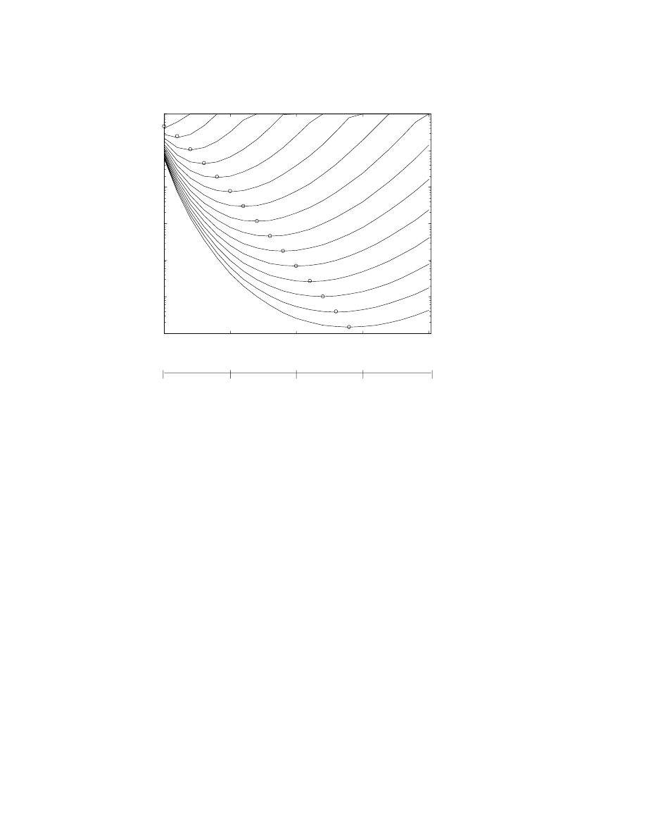
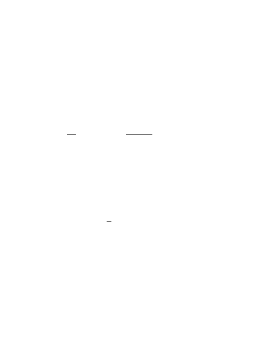
Fig. 1 illustrates the errors in the asymptotic series for the Stieltjes
function (defined in the next section) as a function of N for fifteen
different values of ². For each ², the error dips to a minimum at N
≈
1 /² as the perturbation order N increases. The minimum error for each
N is the “superasymptotic” error.
Also shown is the theoretical prediction that the minimum error
for a given ² is ( π/ (2 ²))
1/2
exp(
−1 / ²) where N
optimum
(²)
∼ 1/² − 1.
For this example, both the exponential factor and the proportionality
constant will be derived in Sec. 5.
The definition of “superasymptotic” makes a claim about the expo-
nential dependence of the error which is easily falsified. Merely by
redefining the perturbation parameter, we could, for example, make
the minimum error be proportional to the exponential of 1/²
γ
where γ
is arbitrary. Modulo such trivial rescalings, however, the superasymp-
totic error is indeed exponential in 1/² for a wide range of divergent
series [30, 72].
The emerging art of “exponential asymptotics” or “beyond-all-orders”
perturbation theory has made it possible to improve upon optimal trun-
cation of an asymptotic series, and calculate quantities “below the radar
screen”, so to speak, of the superasymptotic approximation. It will not
do to describe these algorithms as the calculation of exponentially small
quantities since the superasymptotic approximation, too, has an accu-
racy which is O(exp(
− q / ²) for some constant q. Consequently, Berry
and Howls coined another term to label schemes that are better than
mere truncation of a power series in ²:
Definition 4. A hyperasymptotic approximation is one that achieves
higher accuracy than a superasymptotic approximation by adding one
or more terms of a second asymptotic series, with different scaling
assumptions, to the optimal truncation of the original asymptotic expan-
sion [30]. (With another rescaling, this process can be iterated by
adding terms of a third asymptotic series, and so on.)
All of the methods described below are “hyperasymptotic” in this
sense although in the process of understanding them, we shall acquire
a deeper understanding of the mathematical crimes and genius that
underlie asymptotic expansions and the superasymptotic approxima-
tion.
ActaApplFINAL_OP92.tex; 21/08/2000; 16:16; no v.; p.11
12
John P. Boyd
0
5
10
15
20
10
-6
10
-5
10
-4
10
-3
10
-2
10
-1
10
0
AA
AA
AA
AA
AA
AA
AA
AA
AA
A
A
AA
AA
AA
AA
AA
AA
AA
AA
AA
AA
AA
AA
AA
AA
AA
AA
ε=
1/2
ε=
1/6
ε=
1/7
ε=
1/8
ε=
1/9
ε=
1/10
ε=
1/11
ε=
1/12
ε=
1/13
ε=
1/14
ε=
1/15
ε=
1
ε=
1/3
ε=
1/5
ε=
1/4
N (perturbation order)
1 /
ε
1
6
11
16
21
Errors
Figure 1. Solid curves: absolute error in the approximation of the Stieltjes func-
tion up to and including the N-th term. Dashed-and-circles: theoretical error
in the optimally-truncated or “superasymptotic” approximation: E
N
optimum
(²)
≈
( π/ (2 ²))
1/2
exp(
−1 / ²) versus 1 /². The horizontal axis is perturbative order N for
the actual errors and 1 /² for the theoretical error
But when does a series diverge? Since all derivatives of exp(
−1/²)
vanish at the origin, this function has only the trivial and useless power
series expansion whose coefficients are all zeros:
exp(
−q/²) ∼ 0 + 0² + 0²
2
+ . . .
(2)
for any positive constant q. This observation implies the first of our
four heuristics about the non-convergence of an ²–power series.
Proposition 2 (Exponential Reciprocal Rule). If a function f (²)
contains a term which is an exponential function of the reciprocal of ²,
then a power series in ² will not converge to f (²).
We must use phrase “not converge to” rather than the stronger
“diverge” because of the possibility of a function like
ActaApplFINAL_OP92.tex; 21/08/2000; 16:16; no v.; p.12

Exponential Asymptotics
13
h(²)
≡
√
1 + ² + exp(
−1/²)
(3)
The power series of h(²) will converge for all
|²| < 1, but it converges
to a number different from the true value of h(²) for all ² except ² = 0.
Fortunately, this situation – a convergent series for a function that
contains a term exponentially small in 1/², and therefore invisible to
the power series – seems to be rare in applications. (The author would
be interested in learning of exceptions.)
Milton van Dyke, a fluid dynamicist, offered another useful heuristic
in his slim book on perturbation methods [297]:
Proposition 3 (Principle of Multiple Scales). Divergence should
be expected when the solution depends on two independent length
scales.
We shall illustrate this rule later.
The physicist Freeman Dyson [122] published a note which has been
widely invoked in both quantum field theory and quantum mechanics
for more than forty years [164, 165, 166], [44, 45, 43]. However, with
appropriate changes of jargon, the argument applies outside the realm
of the quantum, too. Terminological note: a “bound state” is a spatially
localized eigenfunction associated with a discrete, negative eigenvalue
of the stationary Schr¨
odinger equation and the “coupling constant”
is the perturbation parameter which multiplies the potential energy
perturbation.
Proposition 4 (Dyson Change-of-Sign Argument). If there are
no bound states for negative values of the coupling constant ², then a
perturbation series for the bound states will diverge even for ² > 0.
A simple example is the one-dimensional anharmonic quantum oscil-
lator, whose bound states are the eigenfunctions of the stationary Schroedinger
equation:
ψ
xx
+
{E − x
2
− ²x
4
}ψ = 0
(4)
When ²
≥ 0, Eq.(4) has a countable infinity of bound states with pos-
itive eigenvalues E (the energy); each eigenfunction decays exponen-
tially with increasing
| x |. However, the quartic perturbation will grow
faster with
| x | than the unperturbed potential energy term, which is
quadratic in x. It follows that when ² is negative, the perturbation will
reverse the sign of the potential energy at x =
±1/(−²)
1/2
. Because
of this, the wave equation has no bound states for ² < 0, that is, no
ActaApplFINAL_OP92.tex; 21/08/2000; 16:16; no v.; p.13

14
John P. Boyd
eigenfunctions which decay exponentially with
| x | for all sufficiently
large
| x |.
Consequently, the perturbation series cannot converge to a bound
state for negative ², be it ever so small in magnitude, because there is
no bound state to converge to. If this non-convergence is divergence (as
opposed to convergence to an unphysical answer), then the divergence
must occur for all non–zero positive ², too, since the domain of conver-
gence of a power series is always
|²| < ρ for some positive ρ as reviewed
in elementary calculus texts.
This argument is not completely rigorous because the perturbation
series could in principle converge for negative ² to something other
than a bound state. Nevertheless, the Change-of-Sign Argument has
been reliable in quantum mechanics [164].
Implicit in the very notion of a “small perturbation” is the idea
that the term proportional to ² is indeed small compared to the rest of
the equation. For the anharmonic oscillator, however, this assumption
always breaks down for
| x | > 1/|²|
1/2
. Similarly, in high Reynolds
number fluid flows, the viscosity is a small perturbation everywhere
except in thin layers next to boundaries, where it brings the velocity
to zero (“no slip” boundary condition) at the wall. This and other
examples suggests our fourth heuristic:
Proposition 5 (Principle of Non-Uniform Smallness). Divergence
should be expected when the perturbation is not small, even for arbi-
trarily small ², in some regions of space.
When the perturbation is not small anywhere, of course, it is impos-
sible to apply perturbation theory. When the perturbation is small
uniformly in space, the ² power series usually has a finite radius of con-
vergence. Asymptotic–but–divergent is the usual spoor of a problem
where the perturbation is small–but–not–everywhere.
We warn that these heuristics are just that, and not theorems. Coun-
terexamples to some are known, and probably can be constructed for
all. In practice, though, these empirical predictors of divergence are
quite useful.
Pure mathematics is the art of the provable, but applied mathemat-
ics is the description of what happens. These heuristics illustrate the
gulf between these realms. The domain of a theorem is bounded by
extremes, even if unlikely. Heuristics are descriptions of what is prob-
able, not the full range of what is possible.
For example, the simplex method of linear programming can con-
verge very slowly because (it can be proven) the algorithm could visit
every one of the millions and millions of vertices that bound the fea-
sible region for a large problem. The reason that Dantzig’s algorithm
ActaApplFINAL_OP92.tex; 21/08/2000; 16:16; no v.; p.14

Exponential Asymptotics
15
has been widely used for half a century is that in practice, the simplex
method finds an acceptable solution after visiting only a tiny fraction
of the vertices.
Similarly, Hotellier proved in 1944 that (in the worst case) the round-
off error in Gaussian elimination could be 4
N
times machine epsilon
where N is the size of the matrix, implying that a matrix of dimension
larger than 50 is insoluble on a machine with sixteen decimal places
of precision. What happens in practice is that the matrices generated
by applications can usually be solved even when N > 1000 [294]. The
exceptions arise mostly because the underlying problem is genuinely
singular, and not because of the perversities of roundoff error.
In a similar spirit, we offer not theorems but experience.
4. Optimal Truncation and Superasymptotics for the
Stieltjes Function
The first illustration is the Stieltjes function, which, with a change of
variable, is the “exponential integral” which is important in radiative
transfer and other branches of science and engineering. This integral-
depending-on-a-parameter is defined by
S(²) =
Z
∞
0
exp(
−t)
1 + ²t
dt
(5)
The geometric series identity, valid for arbitrary integer N,
1
1 + ²t
=
N
X
j=0
(
−²t)
j
+
(
−²t)
N +1
1 + ²t
(6)
allows an exact alternative definition of the Stieltjes function, valid for
any finite N :
S(²) =
N
X
j=0
(
−²)
j
Z
∞
0
exp(
−t) t
j
dt + E
N
(²)
(7)
where
E
N
(²)
≡
Z
∞
0
exp(
−t)(−²t)
N +1
1 + ²t
dt
(8)
The integrals in (3) are special cases of the integral definition of the
Γ-function and so can be performed explicitly to give
S(²) =
N
X
j=0
(
−1)
j
j! ²
j
+ E
N
(²)
(9)
ActaApplFINAL_OP92.tex; 21/08/2000; 16:16; no v.; p.15

16
John P. Boyd
Eqs. (5)-(9) are exact. If the integral E
N
(²) is neglected, then the
summation is the first (N+1) terms of an asymptotic series. Both Van
Dyke’s principle and Dyson’s argument forecast that this series is diver-
gent.
The exponential exp(
−t) varies on a length scale of O(1) where
O() is the usual “Landau gauge” or “order-of-magnitude” symbol. In
contrast, the denominator depends on t only as ²t, that is, varies on a
“slow” length scale which is O(1/²). Dependence on two independent
scales, i. e., t and (²t), is van Dyke’s “Mark of Divergence”.
When ² is negative, the integrand of the Stieltjes function is singular
on the integration interval because of the simple pole at t =
− 1/ ².
This strongly (and correctly) suggests that S(²) is not analytic at ² = 0
as analyzed in detail in [19]. Just as for Dyson’s quantum problems,
the radius of convergence of the ² power series must be zero.
A deeper reason for the divergence of the ²–series is that Taylor–
expanding 1/(1 + ²t) in the integrand of the Stieltjes function is an
act of inspired stupidity. The inspiration is that an integral which can-
not be evaluated in simple closed form is converted to a power series
with explicit, analytic coefficients. The stupidity is that the domain of
convergence of the geometric series is
| t | < 1 / ²
(10)
because of the simple pole of 1/(1 + ²t) at t =
− 1/². Unfortunately,
the domain of integration is semi-infinite. It follows that the Taylor
expansion is used beyond its interval of validity. The price for this math-
ematical crime is divergence.
The reason that the asymptotic series is useful anyway is because
the integrand is exponentially small in the region where the expansion
of 1/(1 + ²t) is divergent. Split the integral into two parts, one on
the interval where the denominator expansion is convergent, the other
where it is not, as
S(²) = S
con
(²) + S
div
(²)
(11)
where
S
con
(²)
≡
Z
1/²
0
exp(
−t)
1 + ²t
dt, S
div
(²)
≡
Z
∞
1/²
exp(
−t)
1 + ²t
dt
(12)
Since exp(
−t)/(1 + ² t) is bounded from above by exp(−t)/2 for all
t
≥ 1 / ², it follows that
S
div
(²)
≤
exp(
−1 / ²)
2
(13)
ActaApplFINAL_OP92.tex; 21/08/2000; 16:16; no v.; p.16

Exponential Asymptotics
17
Thus, one can approximate the Stieltjes function as
S(²)
≈ S
con
(²) + O(exp(
−1 / ²) )
(14)
The magnitude of that part of the Stieltjes function which is inaccesi-
ble to a convergent expansion of 1/(1+² t) is proportional to exp(
−1 / ²).
This suggests that the best one can hope to wring from the asymptot-
ic series is an error no smaller than the order-of-magnitude of S
div
(²),
that is, O(exp(
−1 / ²)).
5. Hyperasymptotics for the Stieltjes Function
It is possible to break the superasymptotic constraint to obtain a more
accurate “hyperasymptotic” approximation by inspecting the error inte-
grals E
N
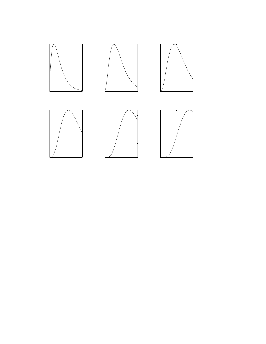
(²), which are illustrated in Fig 5 for a particular value of ².
The crucial point is that the maximum of the integrand shifts to larg-
er and larger t as N increases. When N
≤ 2, the peak (for ² = 1/3)
is still within the convergence disk of the geometric series. For larger
N, however, the maximum of the integrand occurs for T > 1, that is,
for t > 1 /². (Ignoring the slowly varying denominator 1/(1 + ²t), one
can show by differentiating exp(
−t)t
N +1
that the maximum occurs at
t = 1/(N + 1).) When (N + 1)
≥ 1/ ², the geometric series diverges in
the very region where the integrand of E
N
has most of its amplitude.
Continuing the asymptotic expansion to larger N will merely accumu-
late further error.
The key to a hyperasymptotic approximation is to use the informa-
tion that the error integral is peaked at t = 1/². Just as asymptotic
series can be derived by several different methods, similarly “hyper-
asymptotics” is not a single algorithm, but rather a family of siblings.
Their common theme is to append a second asymptotic series, based on
different scaling assumptions, to the “superasymptotic” approximation.
One strategy is to expand the denominator of the error integral
E
N
optimum
(²)
in powers of (t
−1 / ²) instead t. In other words, expand the
integrand about the point where it is peaked (when N = N
optimum
(²)
≈
1 / ²
− 1). The key identity is
1
1 + ²t
=
1
2
{1 +
1
2
(²t
− 1)}
(15)
=
1
2
M
X
k=0
(
−
1
2
)
k
(²t
− 1)
k
ActaApplFINAL_OP92.tex; 21/08/2000; 16:16; no v.; p.17
18
John P. Boyd
0
1
2
0
0.02
0.04
0.06
0.08
T
0
1
2
0
0.01
0.02
0.03
T
0
1
2
0
0.005
0.01
0.015
0.02
0.025
T
0
1
2
0
0.005
0.01
0.015
0.02
0.025
T
0
1
2
0
0.01
0.02
0.03
T
0
1
2
0
0.01
0.02
0.03
0.04
0.05
T
Figure 2. The integrands of the first six error integrals for the Stieltjes function,
E
0
, E
1
, . . . , E
5
for ² = 1/3, plotted as functions of the “slow” variable T
≡ ² t .
S(²) =
N
X
j=0
(
−1)
j
j! ²
j
+
1
2
M
X
k=0
Z
∞
0
exp(
−t)(−²t)
N +1
(
1
− ²t
2
)
k
dt+ H
N M
(²)
(16)
where the hyperasymptotic error integral is
H
N M
(²)
≡
1
2
Z
∞
0
exp(
−t)
1 + ²t
(
−²t)
N +1
(
−
1
2
)
M +1
(²t
− 1)
M +1
dt
(17)
A crucial point is that the integrand of each term in the hyperasymp-
totic summation is exp(
−t) multiplied by a polynomial in t. This means
that the (NM)-th hyperasympotic expansion is just a weighted sum of
the first (N + M + 1) terms of the original divergent series. The change
of variable made by switching from (²t) to (²t
− 1) is equivalent to
the “Euler sum-acceleration” method, an ancient and well-understood
ActaApplFINAL_OP92.tex; 21/08/2000; 16:16; no v.; p.18

Exponential Asymptotics
19
method for improving the convergence of slowly convergent or divergent
series.
Let
a
j
≡ (−²)
j
j!
(18)
S
Superasymptotic
N
≡
[1/²
−1]
X
0
a
j
(19)
where [m] denotes the integer nearest m for any quantity m and where
the upper limit on the sum is
N
optimum
(²) = 1/²
− 1
(20)
Then the Euler acceleration theory [318, 70] shows
S
Hyperasymptotic
0
≡ S
Superasymptotic
N
+
1
2
a
N +1
(21)
S
Hyperasymptotic
1
≡ S
Superasymptotic
N
+
3
4
a
N +1
+
1
4
a
N +2
S
Hyperasymptotic
2
≡ S
Superasymptotic
N
+
7
8
a
N +1
+
1
2
a
N +2
+
1
8
a
N +3
The lowest order hyperasymptotic approximation estimates the error
in the superasymptotic approximation as roughly one-half a
N +1
or
explicitly
E
N
∼ (1/2)(−1)
N +1
(N + 1)!²
N +1
[²
≈ 1/(N + 1)]
(22)
∼
r
π
2²
exp
µ
−
1
²
¶
[² = 1/(N + 1)]
This confirms the claim, made earlier, that the superasymptotic error
is an exponential function of 1 / ².
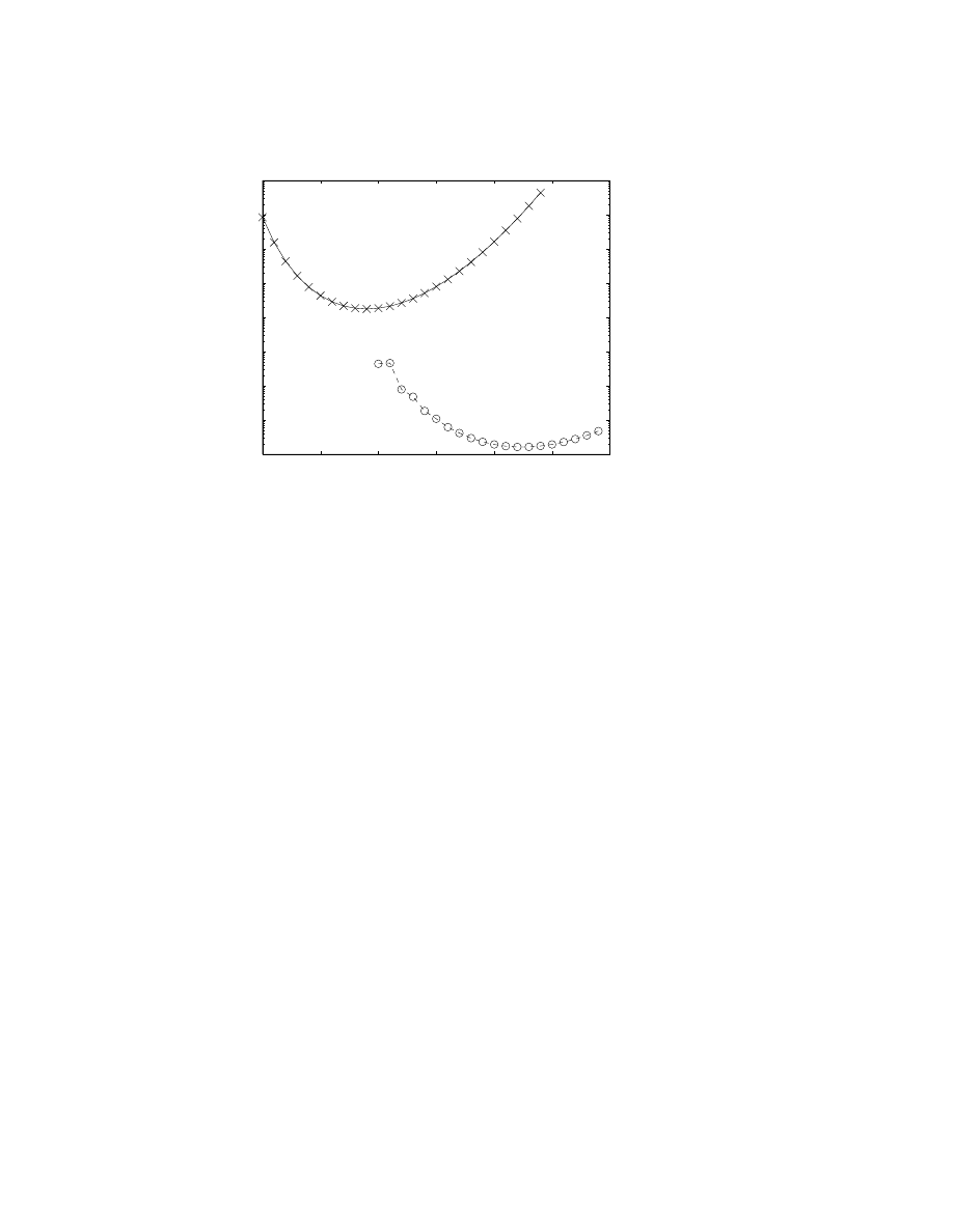
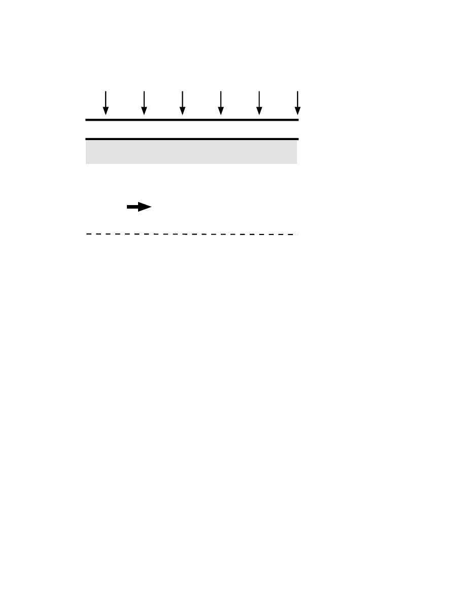
Fig. 3 illustrates the improvement possible by using the Euler trans-
form. A minimum error still exists; Euler acceleration does not elimi-
nate the divergence. However, the minimum error is roughly squared,
that is, twice as many digits of accuracy can be achieved for a given ²
[273, 274], [249], [77].
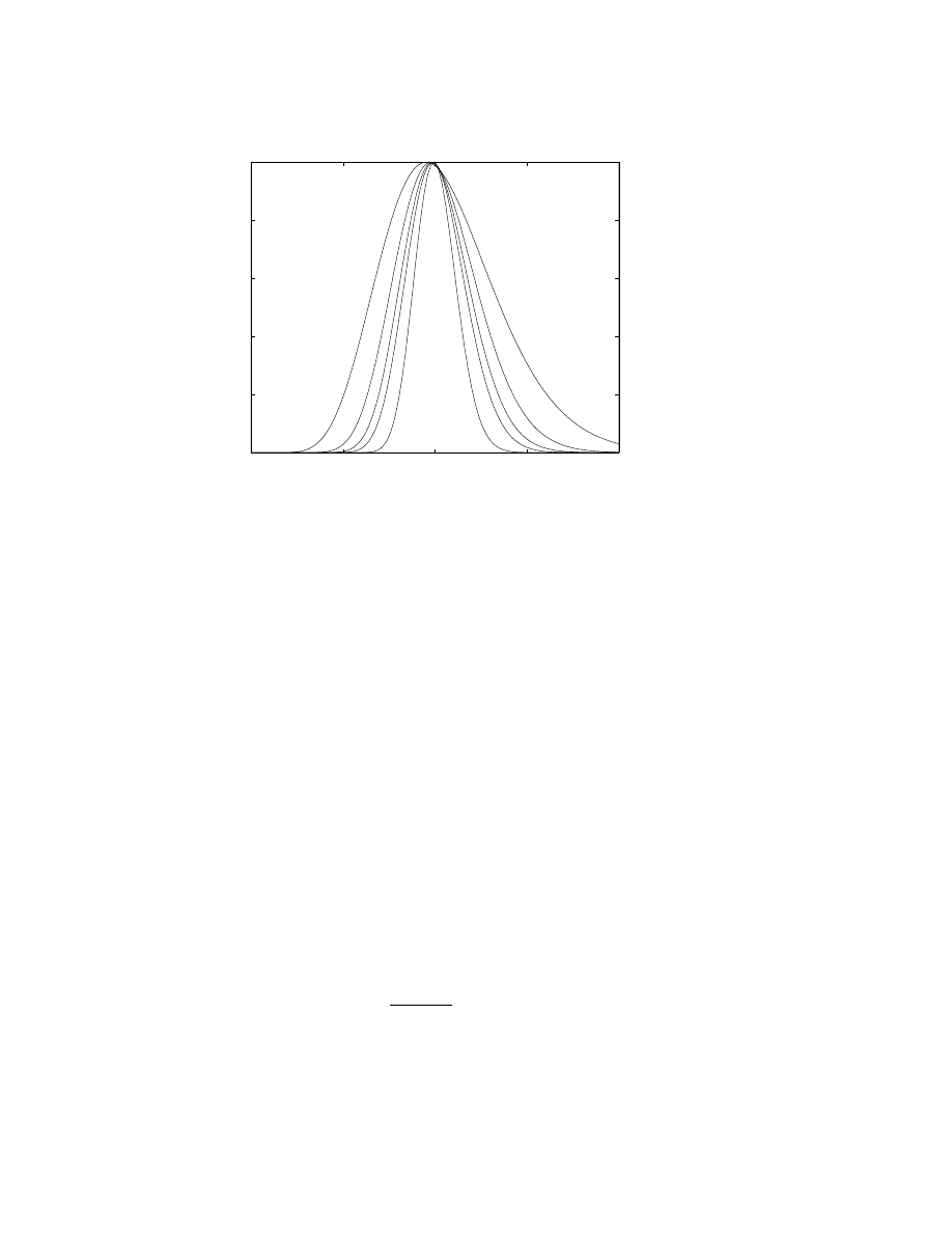
However, a hyperasymptotic series can also be generated by a com-
pletely different rationale. Fig. 4 shows how the integrand of the error
integral E
N
changes with ² when N = N
optimum
(²): the integrand
becomes narrower and narrower. This narrowness can be exploited by
Taylor–expanding the denominator of the integrand in powers of 1
−²t,
which is equivalent to the Euler acceleration of the regular asymptotic
series as already noted. However, the narrowness of the integrand also
implies that one may make approximations in the numerator, too.
ActaApplFINAL_OP92.tex; 21/08/2000; 16:16; no v.; p.19
20
John P. Boyd
0
5
10
15
20
25
30
10
-8
10
-7
10
-6
10
-5
10
-4
10
-3
10
-2
10
-1
10
0
Errors
j
Figure 3. Stieltjes function with ²=1/10. Solid-with-x’s: Absolute value of the abso-
lute error in the partial sum of the asymptotic series, up to and including a
j
where
j is the abscissa. Dashed-with-circles: The result of Euler acceleration. The terms
up to and including the optimum order, here N
opt
(²) = 9, are unweighted. Terms of
degree j > N
opt
are multiplied by the appropriate Euler weight factors as described
in the text. The circle above j = 15 is thus the sum of nine unweighted and six
Euler-weighted terms.
Qualitatively, the numerator resembles a Gaussian centered on t =
1/ ². The heart of the “steepest descent” method for evaluating integrals
is to (i) rewrite the rapidly varying part of the integral as an exponential
(ii) make a change of variable so that this exponential is equal to the
Gaussian function exp(
−z
2
/²) and expand dt/dz, multiplied by the
slowly varying part of the integral (here 1/(1 + ²t(z), in powers of z.
Since this method is described in Sec. 11 below, the details will be
omitted here. The lowest order is identical with the lowest order Euler
approximation.
W. G. C. Boyd (no relation) has developed systematic methods for
integrals that are Stieltjes functions, a class that includes the Stielt-
jes function as a special case[77, 78, 79, 80]. The simpler treatment
described here is based on Olver’s monograph[249] and forty-year old
articles by Rosser[273, 274].
ActaApplFINAL_OP92.tex; 21/08/2000; 16:16; no v.; p.20
Exponential Asymptotics
21
0
0.5
1
1.5
2
0
0.2
0.4
0.6
0.8
1
Integrand
T
ε=1/5
ε=1/80
Figure 4. Integrand of the integral E
N
optimum
(²), which is the error in the regular
asymptotic series truncated at the N –th term, as a function of T
≡ ²t for ² =
1/5, 1/10, 1/20, 1/40, 1/80 in order of increasing narrowness.
6. A Linear Differential Equation
Our second example is the linear problem
²
2
u
xx
− u = −f(x)
(23)
on the infinite interval x
∈ [−∞, ∞] subject to the conditions that
both
|u(x)|, |f(x)| → 0 as |x| → ∞ where the subscripts denote second
differentiation with respect to x, f (x) is a known forcing function, and
u(x) is the unknown. This problem is a prototype for boundary layers
in the sense that the term multiplying the highest derivative formally
vanishes in the limit ²
→ 0, but it has been simplified further by omit-
ting boundaries. The divergence, however, is not eliminated when the
boundaries are.
At first, this linear boundary value problem seems very different
from the Stieltjes integral. However, Eq. (23) is solved without approx-
imation by the Fourier integral
u(x) =
Z
∞
−∞
F (k)
1 + ²
2
k
2
exp(ikx)dk
(24)
ActaApplFINAL_OP92.tex; 21/08/2000; 16:16; no v.; p.21

22
John P. Boyd
where F (k) is the Fourier transform of the forcing function:
F (k) =
1
2π
Z
∞
−∞
f (x) exp(
−ikx)dx
(25)
The Fourier integral (24) is very similar in form to the Stieltjes
function. To be sure, the range of integration is now infinite rather
than semi-infinite and the exponential has a complex argument. The
similarity is crucial, however: for both the Stieljes integral and the
Fourier integral, expanding the denominator of the integrand in powers
of ² generates an asymptotic series. In both cases, the series is divergent
because the expansion of the denominator has only a finite radius of
convergence whereas the range of integration is unbounded.
The asymptotic solution to (23) may be derived by either of two
routes. One is to expand 1/(1 + ²
2
k
2
) as a series in ² and then recall
that the product of F (k) with (
−k
2
) is the transform of the second
derivative of f(x) for any f(x). The second route is to use the method of
multiple scales. If we assume that the solution u(x) varies only on the
same “slow” O(1) length scale as f (x), and not on the “fast” O(1/²)
scale of the homogeneous solutions of the differential equation, then the
second derivative may be neglected to lowest order to give the solution
u(x)
≈ f(x). This is called the “outer” solution in the language of
matched asymptotic expansions.) Expanding u(x) as a series of even
powers of ² and continuing this reasoning to higher order gives
u(x)
∼
∞
X
j=0
²
2
d
2j
f
dx
2j
(26)
This differential equation seems to have little connection to our pre-
vious example, but this is a mirage. For the special case
f (x) =
4
1 + x
2
(27)
the Fourier transform F (k) = 2 exp(
− | k | ) . Using the partial fraction
expansion 1/(1 + ²
2
k
2
) = (1/2)
{1/(1 − i ² k) + 1/(1 + i ² k)}, one can
show that the solution to (23) is
u(x; ²) =
1
1 + ix
½
S
µ
−
i²
1 + ix
¶
+ S
µ
i²
1 + ix
¶¾
+
1
1
− ix
½
S
µ
−
i²
1
− ix
¶
+ S
µ
i²
1
− ix
¶¾
(28)
where S(²) is the Stieltjes function. At x = 0, the solution simplifies
to u(0) = 2
{S(i²) + S(−i²)}. The odd powers of ² cancel, but the even
ActaApplFINAL_OP92.tex; 21/08/2000; 16:16; no v.; p.22
Exponential Asymptotics
23
powers reinforce to give
u(0)
∼ 4
∞
X
j=0
(2j)! (
−1)
j
²
2j
(29)
There is nothing special about the Lorentzian function (or x = 0),
however. As explained at greater length in [61] and [69], the exponential
decay of a Fourier transform with wavenumber k is generic if f (x) is
free of singularities for real x. The factorial growth of the power series
coefficients with j, explicit in (29), is typical of the general multiple
scale series (26) for all x for most forcing functions f (x).
To obtain the optimal truncation, apply the identity 1/(1 + z) =
P
N
j=0
(
−z)
j
+ (
−z)
N +1
/(1 + z) for all z and any positive integer N to
the integral (24) with z = ²
2
k
2
to obtain, without approximation,
u =
N
X
j=0
²
2
d
2j
f
dx
2j
+ (
−1)
N +1
²
2(N +1)
Z
∞
−∞
k
2(N +1)
F (k)
1 + ²
2
k
2
exp(ikx)dk (30)
The N -th order asymptotic approximation is to neglect the integral. For
large N , the error integral in Eq. (30) can be approximatedly evaluated
by steepest descent (Sec. 11 below). The optimal truncation is obtained
by choosing N so as to minimize this error integral for a given ². It is
not possible to proceed further without specific information about the
transform F (k). If, however, one knows that
F (k)
∼ A exp(−µ|k|) as |k| → ∞
(31)
for some positive constant µ where
A denotes factors that vary alge-
braically rather than exponentially with wavenumber, then independent
of
A (to lowest order), the optimal truncation as estimated by steepest
descent is
N
opt
(²)
∼
µ
2 ²
− 1,
² << 1
(32)
and the error in the “superasymptotic” approximation is
¯¯
¯¯
¯¯
u(x; ²)
−
N
opt
X
j=0
²
2
d
2j
f
dx
2j
¯¯
¯¯
¯¯
≤ A
0
exp
µ
−
µ
²
¶
,
² << 1
(33)
where
A
0
denotes factors that vary algebraically with ², i. e., slowly
compared to the exponential, in the limit of small ².
In textbooks on perturbation theory, the differential equation (23) is
most commonly used to illustrate the method of matched asymptotic
ActaApplFINAL_OP92.tex; 21/08/2000; 16:16; no v.; p.23

24
John P. Boyd
expansions. The multiple scales series (26) is the interior or “outer”
solution. To satisfy the boundary conditions
u(
−1) = u(1) = 0
(34)
it is necessary to add “inner” solutions which are functions of the “fast”
variable X = x/². For (23), the exact solution is
u(x; ²) = u
p
(x; ²) + a exp(
−[x + 1]/²) + b exp([x − 1]/²)
(35)
where u
p
(x; ²), the particular solution, is the solution to the same prob-
lem on the infinite interval, already described above, and
a =
−u
p
(
−1; ²) + e
−2/²
u
p
(1; ²)
1
− exp(−4/²)
, b =
−u
p
(1; ²) + e
−2/²
u
p
(
−1; ²)
1
− exp(−4/²)
(36)
The “inner” expansion is just the perturbative approximation to the
exponentials in (35). The matched asymptotics solution is completed
by matching the inner and outer expansions together, term-by-term.
It is important to note that for the finite domain x
∈ [−1, 1], it is
perfectly reasonable to choose a function like g(x) = x
4
/(1 + x
2
), which
is unbounded as
|x| → ∞ and therefore lacks a well-behaved Fourier
transform. However, the hyperasymptotic method can be extended to
such cases by defining the function f in the Fourier integral to be
f (x)
≡ g(x)
1
2
{erf(λ[x − 2]) − erf( λ[x + 2])}
(37)
If the constant λ is large, the multiplier of g differs from 1 by an expo-
nentially small amount on the interval x
∈ [−1, 1] so that f ≈ g on the
finite domain. The modified function f , unlike g, decays exponentially
with
|x| as |x| → ∞ so that it has a well-behaved Fourier transform.
We can therefore proceed exactly as before with f used to generate the
“outer” approximation in the form of a Fourier transform. For exam-
ple, for the particular case g = x
4
/(1 + x
2
), the poles at x =
±i imply
that F (k) decays as exp(
−|k|) so that the optimal truncation and error
bound are the same as for the Lorentzian forcing, f = 4/(1 + x
2
).
Since asymptotic matching is needed only because of the boundaries
(and boundary layers), it is natural to assume that the inner expansion
is the villain, responsible for the divergence of the matched asymptotic
expansions. This is only half-true. In the perturbative scheme,
a
∼ − u
p
(
−1; ²);
b
∼ − u
p
(1; ²)
(38)
to all orders in ² with an error which is O(exp(
−2/²))). The boundary
layers have indeed enforced a minimum error below which the ordi-
nary perturbative scheme cannot go, but it depends on the separation
ActaApplFINAL_OP92.tex; 21/08/2000; 16:16; no v.; p.24

Exponential Asymptotics
25
between the boundaries. Here, the boundary-layer-induced error is only
the square of the minimum error in the power series for u
p
(x; ²) when
f (x) = 4/(1 + x
2
).
The outer solution is a greater villain. Even without boundaries, the
multiple scales series is divergent.
7. Weakly Nonlocal Solitary Waves
“In general, the divergence of series in perturbation theory (while
a good approximation is given by a few initial terms) is usually
related to the fact that we are looking for an object which does
not exist. If we try to fit a phenomenon to a scheme which actually
contradicts the essential features of the phenomenon, then it is not
surprising that our series diverge.”
V. I. Arnold, (1937–)[7], pg. 395.
Solitary waves, which are spatially localized nonlinear disturbances
that propagate without change in shape or form, have been important
in a wide range of science and engineering disciplines. Such diverse
phenomena as the Great Red Spot of Jupiter, Gulf Stream rings in
the ocean, neural impulses, vibrations in polymer lattices, and perhaps
even the elementary particles of physics have been identified, at least
tentatively, as solitary waves; in ten years, most of our phone and data
communications may be through exchange of envelope solitary waves
in fiber optics.
Classic examples of solitary waves decay exponentially fast away
from the peak of the disturbance. In the last few years, as reviewed
in the author’s book [72] and also [56], it has become clear that soli-
tary waves which flunk the decay condition are equally important. Such
“weakly nonlocal” solitary waves decay not to zero, but to an oscilla-
tion of amplitude α, the “radiation coefficient” (Fig. 5). The amplitude
of these oscillations is important because it determines the radiative
lifetime of the disturbance.
The complication is that for many nonlocal solitary waves, the radi-
ation coefficient α is an exponential function of 1/² where ² is a small
parameter proportional to the amplitude of the maximum of the soli-
tary wave. This implies that an ordinary asymptotic series in powers
of ²:
− must fail to converge to the solution.
ActaApplFINAL_OP92.tex; 21/08/2000; 16:16; no v.; p.25
26
John P. Boyd
-20
-10
0
10
20
0
0.1
0.2
0.3
0.4
0.5
0.6
x
u
Core
Wing
Wing
}
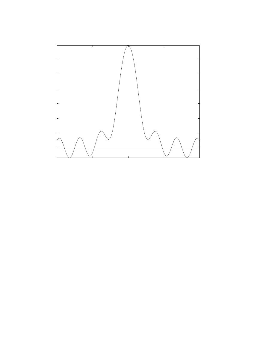
α
Figure 5. Schematic of a weakly nonlocal solitary wave or a forced wave of simi-
lar shape. The amplitude of the “wings” is the “radiation coefficient” α, which is
exponentially small in 1/² compared to the amplitude of the“core”
− must tell us nothing about whether the solitary waves are classical
or weakly nonlocal.
− must be useless for computing α.
However, it is possible to compute the radiation coefficient through a
hyperasymptotic approximation [68],[72].
A full treatment of a weakly nonlocal soliton is too complicated for
an introduction to hyperasymptotics, but it is possible to give the fla-
vor of the subject through the closely-related inhomogeneous ordinary
differential equation studied by Akylas and Yang [5]
²
2
u
xx
+ u
− ²
2
u
2
= sech
2
(x)
(39)
To lowest order in ², the second derivative is negligible compared to
u, just as in our previous example, and the quadratic term is also small
so that
u(x)
∼ sech
2
(x)
(40)
ActaApplFINAL_OP92.tex; 21/08/2000; 16:16; no v.; p.26

Exponential Asymptotics
27
By assuming u(x) may be expanded as a power series in even powers
of ², substituting the result into the differential equation and matching
powers one finds
u(x)
∼
∞
X
j=0
²
2j
u
j
,
u
j
≡
j+1
X
m=1
a
jm
sech
2m
(41)
When this series is truncated to finite order, j
≤ N, all terms in
the truncation decay exponentially with
|x| and therefore so does the
approximation u
N
. In reality, the exact solution decays to an oscil-
lation, just as in Fig. 5. The “wings” are invisible to the multiple
scales/amplitude expansion because the amplitude α of the wings is
an exponential function of 1/².
Boyd shows [68] [with notational differences from this review] that
the residual equation which must be solved at each order is
u
N +1
= r(u
N
)
(42)
where r(u
N
)
≡ −{²
2
u
N
xx
+ u
N
− ²
2
(u
N
)
2
− sech
2
(x)
} is the ”residual
function” of the solution up to and including N -th order. When the
order N = N
optimum
∼ −1/2 + π/(4²), the Fourier transform of the
residual is peaked at wavenumber k = 1/². In other words, when the
series is truncated at optimal order, the neglected second derivative is
just as important as u
N +1
in consistently computing the correction at
next order. The hyperasymptotic approximation is to replace Eq. (42)
by
²
2
u
N +1,xx
+ u
N +1
= r(u
N
)
(43)
for all N > N
optimum
.
The good news is that the nonlinear term in the original forced-
KdV equation is still negligible on the left-hand side of the pertur-
bation equations at each order (though it appears in the residual on
the right-hand side). The bad news is that the equation we must solve
to compute the hyperasymptotic corrections, although linear, does not
admit a closed form solution except in the form of an integral which
cannot generally be evaluated analytically:
²
2
u
N +1
(x) =
Z
∞
−∞
R
N
(k)
1
− ²
2
k
2
exp(ikx)dk
(44)
where R
N
(k) is the Fourier transform of the residual of the N-th order
perturbative approximation.
The Euler expansion cannot help; a weighted sum of the terms of
the original asymptotic series must decay exponentially with
| x | and
ActaApplFINAL_OP92.tex; 21/08/2000; 16:16; no v.; p.27

28
John P. Boyd
therefore will miss the oscillatory wings. The integrand in Eq. 44 is
now singular on the integration interval, rather than off it as for the
Stieltjes function. Indeed, when N
≈ N
optimum
(²), the numerator of
the integrand is largest at
| k |= 1/², precisely where the denominator
is singular! No simple change in the center of the Taylor expansion of
the denominator factor 1/(1
− ²
2
k
2
) will help here.
Fortunately, it is possible to partially solve Eq. 43 in the sense that
we can analytically determine the amplitude of the radiation coefficient
α. Boyd [68] shows that α is just the Fourier transform of the residual
at the points of singularity. The result is an approximation to α(²)
with relative error O(²
2
). This can be extrapolated to the limit ²
→ 0
to obtain
α(²) =
1.558823 + O(²
2
)
²
2
exp
µ
−
π
2²
¶
,
² << 1
(45)
As for the Stieltjes integral, several different hyperasymptotic meth-
ods are available for weakly nonlocal solitary waves and related prob-
lems. The most widely used is to match asymptotic expansions near
the singularities of the solitary wave on the imaginary axis. Originally
developed by Pokrovskii and Khalatnikov [262] for “above-the-barrier”
quantum scattering (WKB theory in the absence of a turning point),
it was first applied to nonlinear problems by Kruskal and Segur [278],
[172]. The book by Boyd [72] reviews a wide number of applications
and improvements to the PKKS method.
Akylas and Yang[5, 323, 324, 325, 327] apply multiple scales per-
turbation theory in wavenumber space after a Fourier transformation.
Chapman, King and Adams[96], Costin[104, 105] and Costin and Kruskal[106,
107], ´
Ecalle[123] have all shown that related but distinct methods can
also be applied to nonlinear differential equations.
8. Overview of Hyperasymptotic Methods
Hyperasymptotic methods include the following:
1. (Second) Asymptotic Approximation of Error Integral or Residual
Equation for Superasymptotic Approximation
2. Isolation Strategies, or Rewriting the Problem so the Exponentially
Small Thing is the Only Thing
3. Resurgence Schemes or Resummation of Late Terms
4. Complex-Plane Matching of Asymptotic Expansions
ActaApplFINAL_OP92.tex; 21/08/2000; 16:16; no v.; p.28

Exponential Asymptotics
29
5. Special Numerical Algorithms, especially Spectral Methods
6. Sequence Acceleration including Pad´e and Hermite-Pad´e Approx-
imants
7. Hybrid Numerical/Analytical Perturbative Schemes
The labels are suggestive rather than mutually exclusive. As shown
amusingly in Nayfeh [229], the same asymptotic approximation can
often be generated by any of half a dozen different methods with seem-
ingly very dissimilar strategies. Thus, the Euler summation gives the
exact same sequence of approximations, when applied to the Stieltjes
function, as making a power series expansion in the error integral for
the superasymptotic approximation.
In the next few sections,we shall briefly discuss each of these general
strategies in turn.
9. Isolation of Exponential Smallness
Long before the present surge of interest in exploring the world of the
exponentially small, some important problems were successfully solved
without benefit of any of the strategies of modern hyperasymptotics.
The key idea is isolation: in the region of interest (perhaps after a
transformation or rearrangement of the problem), the exponentially
small quantity is the only quantity so that it is not swamped by other
terms proportional to powers of ².
A quantum mechanical example is the “WKB”, “phase-integral” or
“Liouville-Green” calculation of “Below-the-Barrier Wave Transmis-
sion”. The goal is to solve the stationary Schroedinger equation
ψ
xx
+
{k
2
− V (² x)}ψ = 0
(46)
subject to the boundary conditions of (i) an incoming wave from the
left of unit amplitude and (ii) zero wave incoming from the right:
ψ
∼ exp(ikx)+α exp(−ikx), x → −∞;
ψ
∼ β exp(ikx), x → ∞
(47)
The goal is to compute the amplitudes of the reflected and transmit-
ted waves, α and β, respectively. If k
2
< max(V (²x)),however, β is
exponentially small in 1/² for fixed k, and α differs from unity by an
exponentially small amount also. Nevertheless, this problem was solved
in the 1920’s as reviewed in Nayfeh [229] and Bender and Orszag [19].
The crucial point is that on the right side of the potential barrier,
the exponentially small transmitted wave is the entire wavefunction.
ActaApplFINAL_OP92.tex; 21/08/2000; 16:16; no v.; p.29
30
John P. Boyd
AAAAAAAAAAAAAAAAA
AAAAAAAAAAAAAAAAA
Porous Wall
Boundary Layer
Inviscid Region
Channel Midline
Flow
}
Pumped Flow
Y=0
Y=1
Figure 6. Schematic of the Berman-Terrill-Robinson problem. Fluid in the channel
flows to the right, driven partly by fluid pumped in through the porous wall. Only
half of the channel is shown because the flow is symmetric with respect to the midline
of channel (dashed)
There is no ambiguity: far to the right, the WKB approximation must
approximate a transmitted, rightgoing wave and nothing else. This, in
an analysis too widely published to be repeated here, allows the analyti-
cal determination of β through standard WKB or matched asymptotics
expansions.
In contrast, standard WKB is quite impotent for determining the
difference between the amplitude of the reflected wave and one because
the large reflected wave swamps the exponentially small correction.
However, α is easily found indirectly by combining the known values
of the incoming and transmitted waves with conservation of energy.
Similarly, WKB gives a good approximation to the bound states and
eigenvalues of a potential well: where the wavefunction is exponentially
small (for large
| x |), there is no competition from terms that are
larger.
A nonlinear example is the “Berman-Terrill-Robinson” or “BTR”
problem, which is interesting in both fluid mechanics and plasma physics
[135, 154, 108, 193, 186, 109]. In its mechanical engineering application,
the goal is to calculate the steady flow in a pipe or channel with porous
walls through which fluid is sucked or pumped at a constant uniform
velocity V . Berman [23] showed that for both the pipe and channel,
the problem could be reduced to a nondimensional, ordinary differen-
ActaApplFINAL_OP92.tex; 21/08/2000; 16:16; no v.; p.30

Exponential Asymptotics
31
tial equation which in the channel case is
² f
Y Y Y
+ f
2
Y
− ff
Y Y
= α
2
(48)
where α is the eigenparameter which must be computed along with
f (Y ). The boundary conditions are
f (1) = 1,
f
Y
(1) = 0,
f (0) = 0,
f
Y Y
(0) = 0
(49)
The small parameter is ² = 1/R where R is the usual hydrodynamics
“Reynolds number” (very large in most applications). Symmetry with
respect to the midline of the channel (at Y = 0) is assumed.
By matching asymptotic expansions, boundary layer to inviscid inte-
rior
(Fig. 6), one can easily compute a solution in powers of ². Unfor-
tunately, the numerical work of Terrill and Thomas [292] showed that
there are actually two solutions for the circular pipe for all Reynolds
numbers for which solutions exist. Terrill correctly deduced that the
two modes differed by terms exponentially small in the Reynolds num-
ber (or equivalently, in 1/²) and analytically derived them in 1973 [291],
quite independently of all other work on hyperasymptotics.
The early numerical work on the porous channel was even more
confusing [265], finding one or two solutions where there are actual-
ly three. Robinson resolved these uncertainties in a 1976 article that
combined careful numerical work with the analytical calculation of the
exponentially small terms which are the sole difference between the two
physically interesting solutions.
The reason that the exponential terms could be calculated with-
out radical new technology is that the solution in the inviscid region
(“outer” solution) is linear in Y plus terms exponentially small in ²:
f (Y )
∼ α(²)Y + γ(²)
½
−3
²
α
+ Y
3
¾
+ . . .
(50)
γ(²) =
±
1
6
µ
2
π²
7
¶
1/4
exp
µ
−
1
4
¶
exp
µ
−
1
4²
¶ ½
1
−
5
4
²
−
253
32
²
2
+ O(²
3
)
¾
(51)
(Note that because of the
± sign, there are two solutions for γ, reflecting
the exponentially small splitting of a single solution (in a pure power
series expansion) into the dual modes found numerically.) It follows
that by making the almost trivial change-of-variable
g
≡ f − αY
(52)
we can recast the problem so that the “outer“ approximation is propor-
tional to exp(
−1/(4²)). Systematic matching of the “inner” (boundary
ActaApplFINAL_OP92.tex; 21/08/2000; 16:16; no v.; p.31

32
John P. Boyd
layer) and “outer” flows gives the exponentially small corrections in
the boundary layer, too, even though there are non-exponential terms
in this region.
Other fluid mechanics cases are discussed in Notes 10 and 11 of the
1975 edition of Van Dyke’s book [298]. Bulakh[85] as early as 1964
included exponentially small terms in the boundary-layer solution to
converging flow between plane walls and showed that such terms will
also arise at higher order in flows with stagnation points. Adamson
and Richey[2] found that for transonic flow with shock waves through
a nozzle, exponentially small terms are as essential as for the BTR
problem.
Happily, there is a widely-applicable strategy for isolating exponen-
tial smallness which is the theme of the next section. The key idea is
that the optimal truncation of the ² power series is always available to
rewrite t he problem in terms of a new unknown which is the difference
between the original u(x; ²) and the optimally-truncated series. Because
this difference δ(x; ²) is exponentially small in 1/², we can determine it
without fear of being swamped by larger terms.
10. Darboux’s Principle and Resurgence
“Evidently, the determination of the remainder [beyond the superasymp-
totic approximation] entails the evaluation of several transcendental
functions. In other words, the calculation of the correction can be
more formidable than that of the original asymptotic expansion.
One is reminded of the dictum, sometimes asserted in physics, that
getting an extra decimal place demands 100 times the effort expend-
ed on the previous one. Fortunately, the multiplying factor is not
so huge in our case but it is perforce appreciable.”
— D. S. Jones (1990) [155] [pg. 261]
Jones’ mildly pessimistic remarks are still true: hyperasymptotics is
more work than superasymptotics and one does have to evaluate addi-
tional transcendentals. However, Dingle showed in a series of articles in
the late fifties and early sixties, collected in his 1973 book, that there is
a suprising universality to hyperasymptotics: a quartet of generic tran-
scendentals suffices to cover almost all cases. The key to his thinking,
refined and developed by Berry and Howls, Olver and many others, is
the following.
Definition 5 (Darboux’s Principle). One may derive an asymp-
totic expansion in degree j for the coefficients a
j
of a series solely from
ActaApplFINAL_OP92.tex; 21/08/2000; 16:16; no v.; p.32

Exponential Asymptotics
33
knowledge of the singularities of the function f (z) that the series rep-
resents. This principle applies to power series [110, 111, 123, 82, 83],
Fourier, Legendre and Chebyshev series [55], and divergent power series
[118]
“Singularity” is a collective terms for poles, branch points and other
points where a complex functionf (z) ceases to be an analytic function
of z. If f (z) is singular, on the same Riemann sheet as the origin, at the
set of points
{z
j
}, then the radius of convergence of the power series
for f (z) is ρ = min
| z
j
|, as proven in most introductory calculus
courses. Darboux showed that if the convergence-limiting singularity
was such that f (z) = (z
− z
c
)
r
g(z) where g(z) is nonsingular at the
convergence-limiting singularity, then the power series coefficients are
asymptotically (if j
6= integer)
a
j
∼ j
−1−r
z
−j
c
{1 + O(1/j)}
(53)
Asymptotics-from-singularities can be extended to logarithms and oth-
er singularities, too. As reviewed in [55], one can derive similar asymp-
totic approximations to the coefficients of Fourier, Chebyshev, Legendre
and other orthogonal expansions from knowledge of the singularities of
f (z).
Dingle [116, 117] realized in the late 50’s that Darboux’s Principle
applies to divergent series, too. If one makes an asymptotic expansion
by performing a power series expansion inside an integral and then
integrating term-by-term, the coefficients of the divergent expansion
will be simply those of the power series in the integration variable
multiplied by the effect – usually a factorial – of the term-by-term
integration. For example, consider the class of functions
f (²)
≡
Z
∞
0
exp(
−t) Φ(²t)dt
(54)
where Φ(z) has the power series
Φ(z) =
∞
X
j=0
b
j
z
j
(55)
then
f (²)
∼
∞
X
j=0
a
j
²
j
;
a
j
= j! b
j
(56)
Because the coefficients of the divergent series
{a
j
} are merely those of
the power series of Φ, multiplied by j!, it follows that the asymptotic
ActaApplFINAL_OP92.tex; 21/08/2000; 16:16; no v.; p.33

34
John P. Boyd
behavior of the coefficients of the divergent series must be controlled by
the singularities of Φ(z) as surely as those of the power series of Φ itself.
In particular, the singularity of the integrand which is closest to t = 0
must determine the leading order of the coefficients of the divergent
expansion. This implies that all f (²) that have a function Φ(z) with
a convergence-limiting singularity of a given type (pole, square root,
etc.) and a given strength (the constant multiplying the singularity)
at a given point z
c
will have coefficients that asymptote to a common
form, even if the functions in this class are wildly different otherwise.
EXAMPLE: The “double Stieltjes” function
SD(²)
≡ S(²) + S(²/2)
(57)
where S(²) is the Stieltjes function described earlier. The asymptotic
series is
SD(²)
∼
∞
X
j=0
a
j
²
j
;
a
j
= (
−1)
j
j!
½
1 +
1
2
j
¾
(58)
The integrand of S(²) is singular at t =
−1/² while that of S(²/2) is
singular twice as far away at t =
−2/². In the braces in Eq. (58), the
first and nearer singularity contributes the one while the rapidly decay-
ing factor 1/2
j
comes from the more distant pole of the integrand, that
of S(²/2). The crucial point is that in the limit j
→ ∞, the coefficients
of the divergent series for the double Stieltjes function asymptote to
those of the ordinary Stieltjes function.
As explained above, the optimal truncation of the ² power series
for the Stieltjes function is to stop at N = [1/²], that is, at the integer
closest to the reciprocal of ²; the error in the resulting “superasymptot-
ic” approximation is proportional to exp(
−1/²). The dominance of the
asymptotic coefficients of the double Stieltjes function by the pole at
t =
−1/² implies that all these conclusions should apply to the optimal
truncation of the divergent expansion for SD(²),too:
SD(²)
∼
N
opt
X
j=0
a
j
²
j
+ O
µq
π/(2²) exp(
−1/²)
¶
;
N
opt
(²) = [1/²]
(59)
where the factor in front of the exponential is justified in [19]. More
important, if we add the error integral for Stieljes function to the
N
opt
(²)-term truncation of the series for the double Stieltjes function,
we should obtain an improved approximation. Since the first neglected
term in the series for SD(²) differs from that included in the Stieltjes
error integral by a relative error of O(²
2N
), the best we can hope for is
to improve upon the superasymptotic approximation by a factor of 2
N
,
ActaApplFINAL_OP92.tex; 21/08/2000; 16:16; no v.; p.34
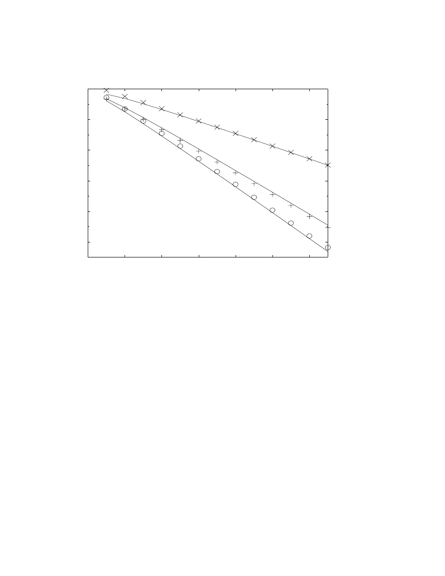
Exponential Asymptotics
35
0
2
4
6
8
10
12
10
−10
10
−8
10
−6
10
−4
10
−2
10
0
1/ε
Superasymptotic
N powers + Terminant
2 N powers + Terminant
Figure 7. Double Stieltjes function: errors in three approximations. x’s: Errors in
optimally-truncated asymptotic series (the “superasymptotic” approximation. Plus-
es: Superasymptotic approximant plus the “terminant”. Circles: Approximation
defined by Eq. (55). Solid curves: Predicted errors, which are respectively the fol-
lowing — (top) q exp(
−1/²), (middle) q exp(−1.693/²), (bottom) q exp(−2/²) where
q(²)
≡ (π/(2²))
1/2
.
which, because N
opt
≈ 1/², can be rewritten as exp(− log(2)/²). Thus,
SD(²)
∼
N
X
j=0
a
j
²
j
+ E
N
(²) + O (exp(
−{1 + log(2)}/²)) ; N(²) = [1/²]
(60)
where E
N
(²) is the error integral for the Stieltjes function defined by
Eq.(8). Fig. 7 shows that the error estimate in Eq. (60) is accurate.
If the location of the second-worst singularity is known — that is,
the pole or branch point of the integrand which is closer to t = 0 than
all others except the one which asymptotically dominates – one can do
better. Since the second pole of SD(²) is at twice the distance of the
first, if we add the next N contributions of the second singularity only
only to the approximation of Eq. (60), the result should be as accurate
ActaApplFINAL_OP92.tex; 21/08/2000; 16:16; no v.; p.35

36
John P. Boyd
as the optimal truncation of a series derived from the second singularity
(i. e., S(²/2) for this example), that is, have an error proportional to
exp(
−2/²):
SD(²)
∼
N
X
j=0
a
j
²
j
+ E
N
(²) +
2 N
X
j=N +1
(
−1)
j
j!
2
j
²
j
+ O
½
exp
µ
−
2
²
¶¾
(61)
Fig. 7 confirms this. (Howls[147] and Olde Daalhuis[241] have devel-
oped improved hyperasymptotic schemes with smaller errors, but for
expository purposes, we have described the simplest approach.)
A key ingredient in Dingle’s strategy is Borel summation. Under
certain conditions [318], a divergent series can be summed by the inte-
gral of exp(
−t) multipied by a function Φ(²t) which is defined to be
that function whose power series has the coefficients of the divergent
series divided by j!. That is to say, the integral in (54) is the Borel
sum of the ² power series for the function f (²) on the left in the same
equation. (We are again reminded of the interplay between different
strategies in hyperasymptotics; a series acceleration method, which is
a hyperasymptotic method in its own right when combined with Pad´
e
approximation of Φ(²t) [“Pad´e-Borel” method [315, 316]], is also a key
justification for a different and sometimes more powerful hyperasymp-
totic scheme.) Dingle’s twist is that he applies Borel summation only to
the late terms in the asymptotic series. The first few terms in the sum
for SD(²) are very different from those of the Stieltjes function; the only
way to obtain the right answer is to sum these leading terms directly
without tricks. Dingle’s key observation is that the late terms, meaning
those neglected in the optimal truncation, are essentially the same as
those for the ordinary Stieltjes function. Thus, the error integral E
N
(²)
for one function, S(²), provides a hyperasymptotic approximation to
an entire class of functions, namely all those of the form of Eq. (54) for
which the convergence-limiting singularity of Φ(z) is a simple pole at
z =
−1.
It might seem as if we would have to repeat the analysis for each
different species of singularity — one family of error integrals when the
singularity is a simple pole, another when the dominant singularity of
Φ is a logarithm and so on. In reality, Dingle shows that for a very wide
range of asymptotic expansions, both from integral representations, the
WKB method, and so on, the coefficients are asymptotically of the form
a
j
∼ q(−1)
j
Γ(j + 1
− β)
ρ
j+1
−β
(62)
for some constants q, ρ and β. The error integral for the Stieltjes func-
tion is almost the theory of everything.
ActaApplFINAL_OP92.tex; 21/08/2000; 16:16; no v.; p.36

Exponential Asymptotics
37
In the next three sections, we describe how Dingle’s theory has been
extended to the method of steepest descent and the mystery of Stokes
phenomenon. A couple of historical, semantic, and notational grace
notes are needed first, however.
The first is that the work of Dingle and others is couched not in
terms of the error integrals E
N
(²) but rather in terms of the following:
Definition 6 (Terminant). A function T
N
(²) is a “terminant” if
it is used to weight the N -th term in an asymptotic series so as to
approximate the exact sum .
The reason for working with terminants instead of errors is mostly
historical. Stieltjes [286] showed that for an alternating series, one could
considerably improve accuracy for both convergent and divergent series
merely by multiplying the last retained term by a weight factor of 1/2.
Airey developed an early (1937) hyperasymptotic method, restricted to
alternating series for which the general term is known, which comput-
ed an improved, N -dependent replacement for Stieltjes’ 1/2 [3]. Later
studies have generally followed this convention. However, terminants
are sometimes more convenient than error integrals as in the smooth-
ing of Stokes phenomenon.
The second comment is that Dingle found it helpful to define four
canonical (approximate) terminants instead of one. One reason is that
the Stieltjes error integral, and the equivalent terminant, have poles on
the negative real axis away from the integration interval, which is the
positive real axis. Stokes phenomenon happens when the poles coincide
with integration interval, which makes it convenient to define a second
terminant. Dingle’s fundamental pair are
Λ
m
(1/²)
≡
1
Γ(m + 1)
Z
∞
0
dt
exp(
−t) t
m
1 + ²t
(63)
Λ
m
(1/²)
≡
1
Γ(m + 1)
P
Z
∞
0
dt
exp(
−t) t
m
1
− ²t
(64)
where P denotes the Cauchy Principal Value of the integral. These two
fission into two more because many expansions proceed in powers of ²
2
rather than ² itself, which makes it convenient to define terminants for
even powers of ², his Π
m
and Π
m
.
Furthermore, newer classes of problems have required additional ter-
minants, as illustrated in Delabaere and Pham[113]. When the hyper-
asymptotic process is iterated so as to add additional terms, with differ-
ent scalings, one needs generalizations of the Dingle terminants called
“hyperterminants”. Olde Daalhuis[240, 242] has given algorithms for
ActaApplFINAL_OP92.tex; 21/08/2000; 16:16; no v.; p.37

38
John P. Boyd
the numerical computation of terminants and hyperterminants. The
need for these generalizations, however, should not obscure the funda-
mental unity of the idea of adding error integrals or terminants that
match the dominant singularity to convert a superasymptotic approx-
imation into a hyperasymptotic approximation.
There is a close parallel between Dingle’s universal terminants for
asymptotic series and the universal error envelopes for Chebyshev and
Fourier spectral methods which were derived by Boyd [55, 59]. For
example, Boyd found that the error envelope was always a linear com-
bination of the same two meromorphic functions (the “Lorentzian” and
“serpentine” functions, defined in [59]), regardless of whether the func-
tion being interpolated was entire, meromorphic, or had logarithmic
singularities. Even when f (x) is nonanalytic but infinitely differentiable
at a point on the expansion interval, and thus has only a divergent
power series about that point, the error envelope is the sum of these
two functions. The reason for the similarity is that Darboux’s Principle
applies to Fourier and Chebyshev series, too. Asymptotically, functions
that are very dissimilar in their first few terms resemble each other more
and more closely in the late terms. One or two terminants can encap-
sulate the error for very different classes of functions, even ones whose
late coefficients are decaying, because of the magic of Taylor expansions
with respect to degree.
11. Steepest Descents
“The resultant series is asymptotic, rather than convergent, because
the range of integration extends beyond the circle of convergence of
[the power series of the metric factor], the radius of this circle being
fixed by the zero of dφ/dt in the complex w-plane lying closest to
the origin.”
— R. B. Dingle [118], pg. 111, with translation of nota-
tion into the symbols used in the section below.
The method of steepest descent is commonly applied to evaluate the
integral
I(z)
≡
Z
exp(zφ(t))dt
(65)
in the limit
| z |→ ∞. As described in standard texts [19], the “saddle
points” or “stationary points”
{t
s
} play a crucial role where these are
defined as the roots of the first derivative of the “phase function” φ(t):
dφ
dt
(t
s
) = 0
(66)
ActaApplFINAL_OP92.tex; 21/08/2000; 16:16; no v.; p.38
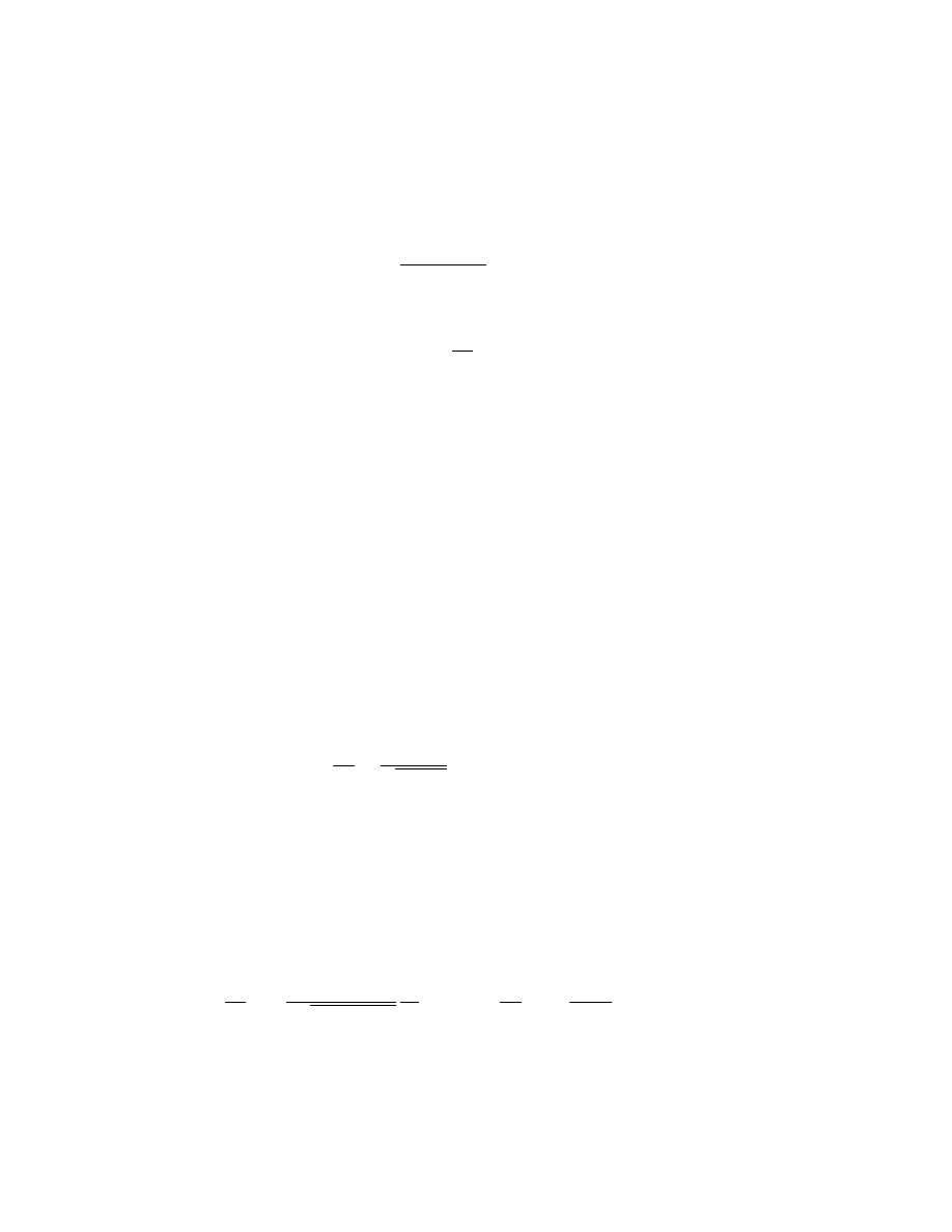
Exponential Asymptotics
39
The path of integration is deformed so as to pass through one or more
saddle points. The next step is to identify the dominant saddle point,
which is the one on the deformed contour of integration for which
<(φ(t
s
)) is largest. Restricting t
s
to the dominant saddle point, one
then makes the exact change-of-variable
w
≡
q
φ(t
s
)
− φ(t)
(67)
so that the integral becomes
I(z) =
Z
exp(
−zw
2
)
dt
dw
(w)
dw
(68)
The final steps are (i) extend the integration interval to the entire real
w-axis and (ii) expand the “metric factor” dt/dw in powers of w and
integrate term-by-term to obtain an exponential factor multiplied by an
inverse power series in the large parameter z. (By setting ² = 1/z, this
series is similar – and similarly divergent – to the ² power series explored
earlier.) We omit details and generalizations because the mechanics are
so widely described in the literature[19, 319].
Unfortunately the standard texts hide the fact that the asymptotic
expansion is based on the same mathematical atrocity as the divergent
series for the Stieltjes function: employing a power series in the inte-
gration variable with a finite radius of convergence under integration
over an infinite interval. Hyperasymptotics is greatly simplified by the
following.
Theorem 1 (Singularities of the Steepest Descent Metric Function).
If an integral of the form of Eq.(65) is transformed by the mapping
Eq. (67) into the integral over w, Eq. (68), then the metric factor dt/dw
has branch points of the form
dt
dw
=
g(w)
√
w
− w
s
+ h(w)
(69)
where g(w) and h(w) are analytic at w = w
s
. All such points w
s
are
the images of the saddle points t
s
under the mapping w(t); conversely,
the metric factor is singular at all points w
s
which are images of saddle
points except for w = 0. The metric factor may also be singular with
singularities of more complicated type at points w which are images of
points where the “phase factor” φ(t) is singular.
PROOF: The first step is to differentiate the definition of the map-
ping Eq.(67) to obtain
dw
dt
=
−
1
2
p
φ(t
s
)
− φ(t)
dφ
dt
;
⇐⇒
dt
dw
=
−2
w
dφ/dt
(70)
ActaApplFINAL_OP92.tex; 21/08/2000; 16:16; no v.; p.39

40
John P. Boyd
This shows that the metric factor can be singular only at the w-images
of those points t in the original integration variable where (i) φ(t) is
singular or (ii) saddle points where by the very definition of a saddle
point, dφ/dt = 0 and the denominator of the right-hand side of Eq.(70)
is zero. This is really just a restatement of the implicit function of
elementary calculus, which states that if dw/dt is non-zero at a point,
then the inverse function t(w) exists and is analytic at that point and
its derivative dt/dw = 1/(dw/dt). The point w = 0 is exceptional
because the numerator of the right-hand side (w) cancels the zero in
the denominator.
To obtain an expression for dt/dw in the neighborhood of a saddle
point, we expand w(t) about the saddle point t = t
s
. The constant w
s
can be moved to the left side of the equation and the linear term is
zero because dw/dt is zero at the saddle point. Taking the square root
gives
√
w
− w
s
= (t
− t
s
)
s
1
2
d
2
w
dt
2
(t
s
)
{1 + O(t − t
s
)
}
(71)
It follows that dt/dw is proportional to 1/
√
w
− w
s
near the saddle
point, which demonstrates the theorem.
Denote the image-of-a-saddle-point of smallest absolute value by
w
min
. The coefficients b
j
of the power series of the integrand will
then asymptote, for sufficiently high degree j, to those of a constant
times 1/
√
w
− w
min
; the contributions of the singularities that are more
remote in the complex w-plane will decrease exponentially fast with
j compared to the contribution of the square root branch point at
w = w
min
. Applying the binomial theorem to compute the power series
coefficients of the square root singularity and then integrating term-
by-term shows that the coefficients a
j
of the asymptotic series for the
integral itself will asymptote for large j to
a
j
∼ q
Γ(j + 1/2)
| w
min
|
j+1/2
(72)
where the constant q is proportional to g(w
min
) in the theorem. Dingle
[118], pg. 457, gives the basic terminant (with some changes in notation)
T
N
∼ q
0
Λ
N
−1
(
−F ) + q
2
Λ
N
−2
(
−F ) + q
4
Λ
N
−3
(
−F ) + . . .
(73)
where the q
2j
are functions of Dingle’s “chief singulant” F , which in
our notation is
F
≡ zw
2
min
(74)
and q
2j
∼ O(F
j
) This situation is more complicated than for the dou-
ble Stieltjes function in that we have a series of terminants, rather
ActaApplFINAL_OP92.tex; 21/08/2000; 16:16; no v.; p.40
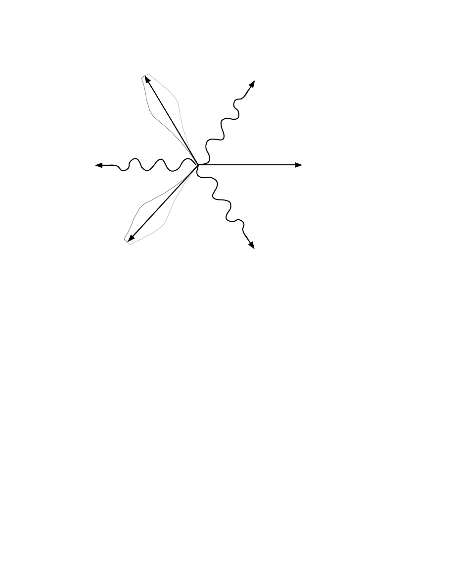
Exponential Asymptotics
41
,,,
,,,,
,,
yyy
yyyy
yy
zzz
zzz
z
{{
{{{
{{{
{
|
|||
|||
,
,,,
,,,,
,
y
yyy
yyyy
y
z
zzz
zzz
z
{{
{{{
{{
||
|||
|||
,
,,
,,,
,,
y
yy
yyy
yy
zzz
zz
zz
{{
{{{
{{
{
|
|||
|||
,
,,
,,,
,
y
yy
yyy
y
z
zzz
zz
zz
{{
{{{
{{{
||
|||
||
Stokes line
Anti-Stokes line
Figure 8. Stokes Lines (Monotonic Growth/Decay) and anti–Stokes Lines (Pure
Oscillation) for the Airy Functions Ai and Bi. The shaded regions show the transition
zone for the Stokes’ multiplier of Ai, that is, the regions where it varies from 1 to 0
as an error function. The positive real axis is a Stokes Line for Bi but not Ai. The
shaded regions narrow for large
|z| because for the Airy function, the width of the
transition zone, expressed in terms of the angle θ
≡ arg(z), decays as |z|
−3/4
.
than a single terminant. (Each term of the expansion of dt/dw in half-
integral powers of w
− w
min
will generate its own contribution to the
terminant series.) The underlying ideas remain simple even though the
algebraic complexity rapidly leaves one muttering: “Thank heavens for
Maple! [and similar symbolic manipulation languages like Mathemati-
ca, Reduce and so on].”
12. Stokes Phenomenon
“ about the present title [Divergent Series], now colourless, there
hung an aroma of paradox and audacity.”
— Sir John E. Littlewood, (1885-1977)[139]
Stokes phenomenon has contributed much to the “aroma of paradox
and audacity” of asymptotic series. It is easiest to explain by example.
The Airy function Ai(z) asymptotes for large positive z to the prod-
uct of a decaying exponential with a series in inverse powers of z
3/2
. For
ActaApplFINAL_OP92.tex; 21/08/2000; 16:16; no v.; p.41
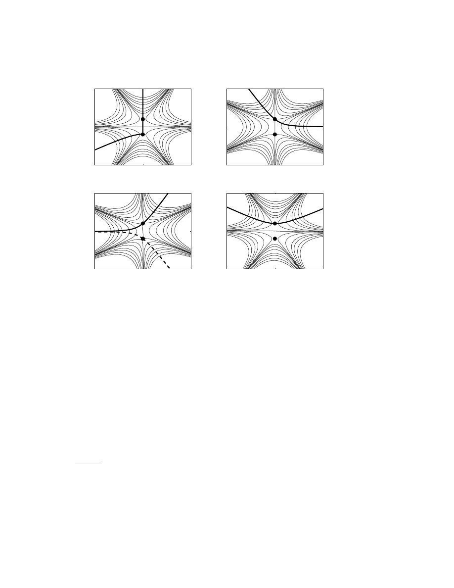
42
John P. Boyd
-5
0
5
-5
0
5
ℑ
(t)
θ
= 2
π
/3
-5
0
5
-5
0
5
ℑ
(t)
θ
=
π
/3
-5
0
5
-5
0
5
ℑ
(t)
ℜ
(t)
θ
=
π
-5
0
5
-5
0
5
ℑ
(t)
ℜ
(t)
θ
=0
Figure 9. Steepest descent paths of integration in the complex plane of the original
integration variable t for four different values of z. The two saddle points are marked
by black discs. The contours of log(
| exp(z
3/2
i
©
t + t
3
/3
ª
)
|) from are also shown
For θ = π [negative real z-axis, lower left panel], the integration contour comes from
large t in the upper right quadrant, returns to infinity along the negative imaginary
t-axis, and then returns to pass through the right saddle point and depart to infinity
via the lower right t-quadrant.
negative real z, the Airy function is real and oscillatory; approximated
by the product of a cosine with a inverse power series plus a sine with
a different inverse power series. However, the multiplier of the leading
inverse power, the cosine, is the sum of two exponentials. If we track
the asymptotic approximation for fixed
| z | as θ = arg(z) varies from
0 to π, one exponential must somehow metamorphosize into two.
The classical analysis hinges on two species of curves in the complex
z-plane: “Stokes lines”, where the exponentials grow or decay without
oscillations, and “anti-Stokes” lines where the exponentials oscillate
without change in amplitude.
1
(Fig. 8.) Stokes’ own interpretation is
1
We employ the convention of Heading, Dingle, Olver, and Berry, but other
authors such as Bender and Orszag reverse the meaning of “Stokes” and “anti-
Stokes”.
ActaApplFINAL_OP92.tex; 21/08/2000; 16:16; no v.; p.42
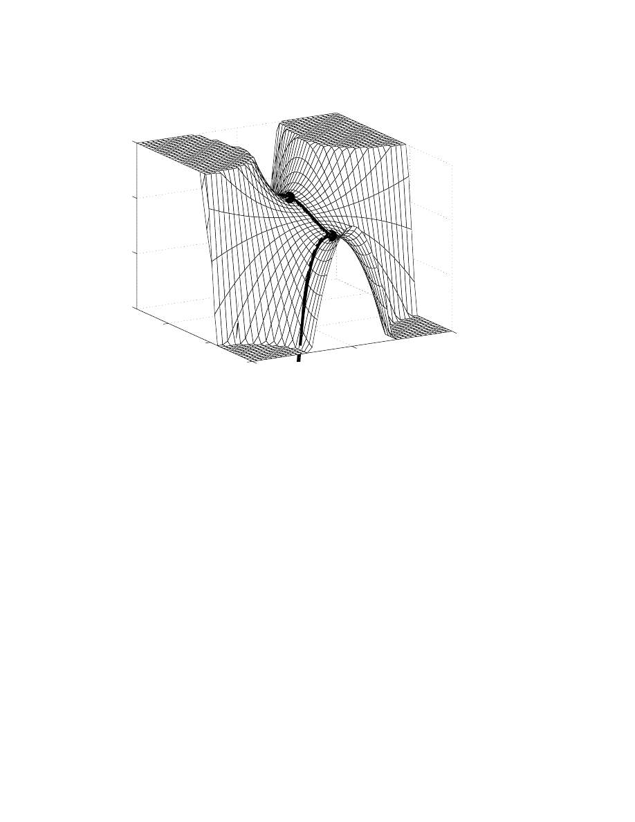
Exponential Asymptotics
43
-5
0
5
-2
0
2
-10
-5
0
5
ℜ
(t)
ℑ
(t)
Figure 10. A surface plot of log(
| exp(z
3/2
φ)
|) for the Airy integral for arg(z) =
2π/3, that is, on the Stokes line. The steepest descent path is marked by the heavy
solid line; the disks denote the two saddle points at t
s
=
±i. The surface has been
truncated at the vertical axis limits for graphical clarity.
that the coefficient of the “recessive” (decaying) exponential jumps dis-
continuously on the Stokes line (for Ai(z), at arg(z) =
±2π/3), that
is, where this exponential is smallest relative to the “dominant” expo-
nential that grows as
| z | increases along the Stokes line. As the nega-
tive real axis (an anti-Stokes line) is approached, the two exponentials
become more and more similar until finally both are purely oscillatory
with coefficients of equal magnitude on the anti-Stokes line itself.
The annoying and unsatisfactory part of this discontinuous jump is
that the Airy function itself is an entire function, completely free of
all jumps, infinities and pathologies of all kinds except at
| z |= ∞.
Sir Michael Berry has recently smoothed this “Victorian discontinu-
ity”, to quote from one of his papers, by combining Dingle’s ideas with
the standard and long-known asymptotic approximation to an inte-
gral when the saddle point and a pole nearly coincide. To understand
Berry’s jump-free hyperasymptotics, we need some preliminaries.
ActaApplFINAL_OP92.tex; 21/08/2000; 16:16; no v.; p.43

44
John P. Boyd
First, let us represent the solution by an integral which can be
approximated by the method of steepest descent for large z. (Berry’s
smoothing is equally applicable to WKB approximations to differential
equations and a wide variety of other asymptotics, but steepest descent
is the most convenient for explaining the concepts.)
The integral representation for the Airy function is
Ai(z)
≡
z
1/2
2π
Z
C
exp
³
z
3/2
n
i (t + t
3
/3)
o´
dt
(75)
where
C is a contour that originates at infinity at an angle arg(t) =
(5/6)π
− (1/2) arg(z) and returns to infinity at arg(t) = (1/6)π −
(1/2) arg(z).
Fig. 9 shows the steepest descent paths of integration for the Airy
integral representation. As explained in the preceding section, the eas-
iest way to generate the coefficients of the asymptotic series is to begin
with a change-of-coordinate to a new integration variable w. To illus-
trate the key topological ideas, however, it is perhaps more illuminating
to illustrate the steepest descent path in the t
− plane as we have done
in the figure. In either plane, the path of integration is deformed so as
to pass through a saddle point, and then curve so that at each point t
on the path,
=(zφ(t
s
)) =
=(zφ(t
s
)). This condition that the phase of
the integrand matches that of the saddle point ensures that the mag-
nitude of the integrand decreases as steeply as possible from its local
maximum, i. e., that the curve is really is a path of “steepest descent”.
As a student, I was much puzzled because my texts and teachers
expended a lot of energy on determining the exact shape of the steepest
descent contour even though it does not appear explicitly in the answer,
even at higher order! The steepest descent path is actually important
only for topological reasons: it is essential to know which saddle points
lie on the path, but the shape of the contour is otherwise irrelevant.
For the Airy function, for example, there are two saddle points for
all z but only one is on the contour for large positive z. As the argument
of z varies, however, the steepest descent paths in the t (or w) planes
must vary also. For some z, the steepest descent path through one
saddle point must collide with the other; this happens precisely on the
Stokes lines.
As shown in Fig. 9, the Stokes lines are a change in the topology of
steepest descent paths: a single saddle point on the contour on one side
of the Stokes line, two saddle points on the other side of the Stokes
line and on the Stokes line itself. Thus, Berry’s title for one of his arti-
cles, “Smoothing a Victorian discontinuity”, is a bit misleading since
the discontinuity is not removed in a topological sense. The jump is,
however, smoothed numerically.
ActaApplFINAL_OP92.tex; 21/08/2000; 16:16; no v.; p.44

Exponential Asymptotics
45
Parenthetically, note that at the Stokes line itself (arg(z) = 2π/3
for Ai(z)), the steepest descent path descends from one saddle point
directly to another saddle point, then makes a right angle turn and
then continues to descend monotonically from the second saddle point
(Fig. 10). For arg(z) > 2π/3, the steepest descent contour from one
saddle point does not runs off to infinity parallel to the negative imagi-
nary axis. To be continuous and still terminate at
∞ exp(iπ/6), howev-
er, the contour must return and pass through the second saddle point.
At arg(z) = π, the contributions of both saddle points are equal.
The properties of Stokes lines may be summarized as follows:
1. There are TWO saddle points on the steepest descent integration
path in the t-plane.
2.
={z(φ(t
+
)
− φ(t
−
)
} = 0 where t
+
and t
−
are the two saddle points
on the steepest descent contour and where φ(t) is the steepest
descent phase function defined by Eq. 65.
3. The terminants for the series each have a simple pole on the real
w-axis, which is the integration interval after the usual steepest
descent change of variable, the poles being at the saddle point
which contributes the “recessive” saddle point.
4. The terms b
j
of the asymptotic inverse power series are, for suffi-
ciently large degree j, all of the same sign.
When there is a discontinuity in asymptotic form, the first three prop-
erties are each equivalent definitions of a “Stokes line”.
The proofs of these assertions and also generalizations of Stokes phe-
nomenon to solutions of nonlinear differential equations and so on are
given by the theory of “resurgence”. ´
Ecalle[123] invented “resurgence”
[123] and the formalism of the “alien calculus” and “multisummabil-
ity”. This has been extended by a group that includes Voros, Pham,
Sternin, Shatalov, Delabaere, and others too numerous to list. The
monograph by Sternin and Shatalov[285] and the collection of articles
edited by Braaksma[83] are good summaries. (Berry, who was visiting
Pham when he developed his smoothing scheme, was strongly influ-
enced by ´
Ecalle’s three-volume book and the follow-up work of the
“French school”.) The alien calculus and multisummability theory are
very general but accordingly also very abstract. Berry and Howls, Olde
Daalhuis and Olver, Costin, Kruskal, Hu and others have developed
simplified variants of resurgence and applied them to concrete prob-
lems in special functions and physics.
As shown by the sheer length of the Table IV, which is a selected
bibliography of works on resurgence and Stokes phenomenon, it is quite
ActaApplFINAL_OP92.tex; 21/08/2000; 16:16; no v.; p.45

46
John P. Boyd
unfeasible to summarize this powerful theory here. (Prof. ´
Ecalle’s pio-
neering treatise is in three volumes!) Still, one can give a little of the
flavor of resurgence.
One key concept is what one might call “saddle point democracy”.
Instead of focusing in quickly on one or two dominant saddle points
(on the steepest descent path), resurgence treats all saddle points on
an equal footing. One may define an integral passing through an arbi-
trary saddle point; the coefficients of the steepest descent expansion
about that point encodes the expansions about all the other saddle
points. Furthermore, the late terms in the asymptotic expansion about
a dominant saddle point can be expressed in terms of the early terms of
a subdominant series, and vice-versa. The reason is that the late terms
in the expansion about the dominant saddle point are controlled, via
Darboux’s Principle, by the singularities created by the other saddle
points.
13. Smoothing Stokes Phenomenon: Asymptotics of the
Terminant
“Having these new techniques [hyperasymptotics], I would like to
hear from anybody who needs the Airy function to twenty decimals,
but am not expecting an early call.”
— Berry (1991) [30] [pg. 2.]
Berry’s amusing comment is a frank admission that the smooth-
ing of the discontinuity along a Stokes line is not a matter of great
arithmurgical significance. The term that changes dramatically in the
neighborhood of the Stokes line is exponentially small compared to the
sum of the asymptotic series. However, the smoothing does provide
deep insights into the interlocking systems of caverns — interlocking
systems of expansions about different saddle points and branch points
— that lie beneath the surface of asymptotic approximations.
The numerical smoothing of the discontinuity along a Stokes lines
is based on the following ideas which will be explained below:
1. The exponentially small Stokes multiplier
M can be isolated by
subtracting the optimal truncation of the standard asymptotic
series for f (z) from it so that the multiplier is no smaller than
the other terms left after the subtraction.
2. The subdominant saddle point, the one whose Stokes multiplier is
to change, lies directly on the steepest descent path leading down
from the dominant saddle point when z or ² is on the Stokes line.
ActaApplFINAL_OP92.tex; 21/08/2000; 16:16; no v.; p.46

Exponential Asymptotics
47
3. When the asymptotic approximation for f (z) is optimally trun-
cated, the saddle point of the integral representation of Dingle’s
terminant will coincide with the subdominant saddle point and
therefore with the pole of the integrand
4. The method of steepest descent, applied to the integrand of the
terminant, replaces the integrand’s sharp peak at its saddle point
with a Gaussian function, thereby reducing the asymptotics of the
terminant to that of a Gaussian divided by a simple pole at the
origin.
5. If we allow the small parameter ² or the equivalent large parameter,
z = 1/², to move a little way δ off the Stokes line, the terminant
integral becomes the Fourier transform of a Gaussian divided by a
pole at (or very near) the maximum of the Gaussian
6. The Fourier transform of a Gaussian divided by a pole is that of
the integral of the Fourier transform of the Gaussian, which is the
error function erf.
To illustrate these ideas, define the “singulant” F via
F
≡ ={z(φ(t
+
)
− φ(t
−
))
}
(76)
where t
+
and t
−
are the two saddle points on the steepest descent
contour and where the a
j
are the coefficients of the inverse power series.
(The real part of the difference between zφ(t) at the two points is zero
along a Stokes line, and this can be used to define a Stokes line.) The
singulant is proportional to some positive power of the large parameter
z so that the inverse power series in z can be expressed as inverse
powers of F .
The Stokes multiplier
M may then be defined by
f (z)
∼ exp(zφ(t
+
))
σ
+
(z)
N
opt
(z)
X
j=0
a
j
F
−j+β−1
+ i
M σ
−
(z) exp(
−F )
(77)
where N
opt
denotes the optimal truncation of the asymptotic series for
a given z, σ
±
(z) are slowly varying factors of z (usually proportional
to a power of z rather than an exponential), β depends on the class
of asymptotic approximation, and the coefficients have been scaled so
that a
0
= 1 by absorbing factors into σ
±
if necessary. (For steepest
descent as discussed here, β = 1, but other values do occur when the
integral involves a contribution from an endpoint of integration interval
ActaApplFINAL_OP92.tex; 21/08/2000; 16:16; no v.; p.47

48
John P. Boyd
or certain other classes of asymptotics[25].) This definition is equivalent
to
M ≡ − i
exp(F )
σ
−
(z)
f (z) exp(
−zφ(t
+
))
− σ
+
(z)
N
opt
(F )
X
j=0
a
j
F
−j+β−1
(78)
Replacing f (z) exp(
−zφ(t
+
)) by the infinite asymptotic series and sub-
tracting
M ∼ − i exp(F )
σ
+
(z)
σ
−
(z)
∞
X
j=N
opt
(F )+1
a
j
F
−j+β
(79)
Note F is real and positive on the Stokes line.
The next step is to sum the series for the Stokes multiplier via Borel
summation. The follow-up is crucial: instead of employing the exact
power series coefficients a
j
in the Borel sum, we use the asymptotic
approximation to them as j
→ ∞. This is legitimate since only late
terms, i.e., those for j > N
opt
(F ), appear in the sum. This approximates
the Stokes multiplier in terms of Dingle’s singular terminant Λ
N
(F ).
To illustrate this general strategy, we shall return to the specific
example of the Airy function, which has the asymptotic approximation
Ai(z)
∼ z
−1/4
1
2
√
π
{E
−
+ i
M E
+
}
(80)
where
E
±
≡
exp(
±(2/3)z
3/2
)
Γ(5/6)Γ(1/6)
∞
X
n=0
Γ(n + 5/6)Γ(n + 1/6)
Γ(n + 1) (
∓F )
n
(81)
The Stokes’ multiplier
M is zero when arg(z) = 0 and is unity when
arg(z) = π.
Dingle’s singulant is defined by
F
≡ −
4
3
z
3/2
(82)
which as always is the difference between the arguments of the two
exponentials in the asymptotic approximation. Note the sign conven-
tion: F is negative when z and ζ are real and positive.
If the coefficients of the asymptotic series for E
−
, which is the dom-
inant exponinant exponential near the Stokes line at arg(z) = (2/3)π,
ActaApplFINAL_OP92.tex; 21/08/2000; 16:16; no v.; p.48

Exponential Asymptotics
49
are denoted by a
j
, then the argument given above implies that
M ∼ − i exp(F )
∞
X
j=N
opt
(F )+1
a
j
F
−j
(83)
∼ − i exp(F )
∞
X
j=N
opt
(F )+1
1
2 π
(j
− 1)! F
−j
(84)
∼ −
i
2 π
Z
∞
0
exp(F (1
− t)) t
N
opt
1
1
− t
dt
(85)
In the second line, we have replaced the a
j
by their asymptotic approx-
imation as j
→ ∞ [derived through the large degree asymptotics of
the gamma functions plus the identity Γ(1/6)Γ(5/6) = 2π]. The third
line was derived from the second by taking the Borel sum of the series,
which happens to be an integral with an integrand that can be written
down explicitly. We can check that the integral is correct by expanding
the integrand about t = 0 and then integrating term-by-term. The inte-
gral is, with a change in integration variable, proportional to Dingle’s
singular terminant.
The integral is not completely specified until one makes a choice
about how to deal with the pole on the path of the integration. Since
we know that for the Airy function, Stokes’ multiplier must increase
from 0 for real, positive z to 1 for real, negative z, the proper choice is
to indent the path of integration above the pole.
The integral is also not fully determined until the optimal truncation
N
opt
has been identified. However, the coefficients asymptotic series for
E
−
, which is the multiplier of the exponential which is dominant near
the Stokes line arg(z) = 2π/3, are asympotically factorials, just the
same as for the Stieltjes function (Eq. (81)). This implies that our
earlier analysis for S(²) applies here, too, to suggest
N
opt
=
|F |
(86)
When F is real and positive, that is, when z is on the Stokes line,
the factor
χ
≡ exp(F (1 − t)) t
N
opt
= exp
{F (1 − t) + N
opt
log(t)
}
(87)
has its maximum at t = 1, which coincides with the singularity of the
factor 1/(1
−t) which is rest of integrand for the Stokes multiplier. This
coincidence of the saddle point with the pole requires only a slight
modification of standard descent to approximate
M near the Stokes
line. Wong[319](pg. 356-360) gives a good discussion, attributing the
original analysis to van der Waerden [296].
ActaApplFINAL_OP92.tex; 21/08/2000; 16:16; no v.; p.49

50
John P. Boyd
The key idea is to expand the factor χ as a power series about t = 1,
rather than the saddle point, which is slightly shifted away from t = 1
when
=(F ) 6= 0. Let T ≡ t − 1 and F ≡ F
r
+ iF
im
. Furthermore,
since the integral is strongly peaked about T = 0, the lower limit
of integration has been extended from T =
−1 to −∞. The Stokes
multiplier is approximately
M = −
i
2 π
Z
∞
−∞
exp
µ
−i F
im
T
− −
1
2
F
2
r
T
2
¶
1
T
dT
(88)
where terms of O(T
3
) in the exponential have been neglected.
This approximation is just the Fourier transform of a Gaussian func-
tion (exp(
−(1/2)F
2
r
T ), divided by iT . The identity
lim
δ
→0
−i
2π
Z
∞
−∞
exp(
−ikx) exp(−a
2
k
2
)
1
(k + i δ)
dk =
1
2
+
1
2
erf
µ
x
2a
¶
(89)
shows that the Stokes multiplier is
M =
1
2
+
1
2
erf
µ
F
im
√
2F
r
¶
(90)
Fig. 11 shows that this approximation is very accurate.
The error function does not cover all cases; Chapman[95] has shown
that other smoothing functions are needed in some circumstances. How-
ever, the complementary error function does remove the “Victorian
discontinuity” of Stokes for a remarkably wide class of functions.
14. Matched Asymptotic Expansions in the Complex Plane:
The PKKS Method
In “above-the-barrier” quantum scattering, there are no turning points
where the coefficient of the undifferentiated term in the Schr¨
odinger
equation is zero except at complex values of the spatial coordinate.
When there are real-valued turning points, it was discovered in the
1920s that the scattering — including the exponentially small transmis-
sion through the barrier – can be computed by means of the so-called
turning point connection formulas. (The transmission coefficient can be
calculated without heroics because the exponentially small transmitted
wave is the whole solution on the far side of the barrier, isolating it
from terms proportional to powers of ² as noted earlier.) Later, it was
shown that the connection formulas are really just a special case of the
method of matched asymptotic expansions [229, 20, 21]. The solution
in the neighborhood of the turning point can be expressed (to lowest
ActaApplFINAL_OP92.tex; 21/08/2000; 16:16; no v.; p.50
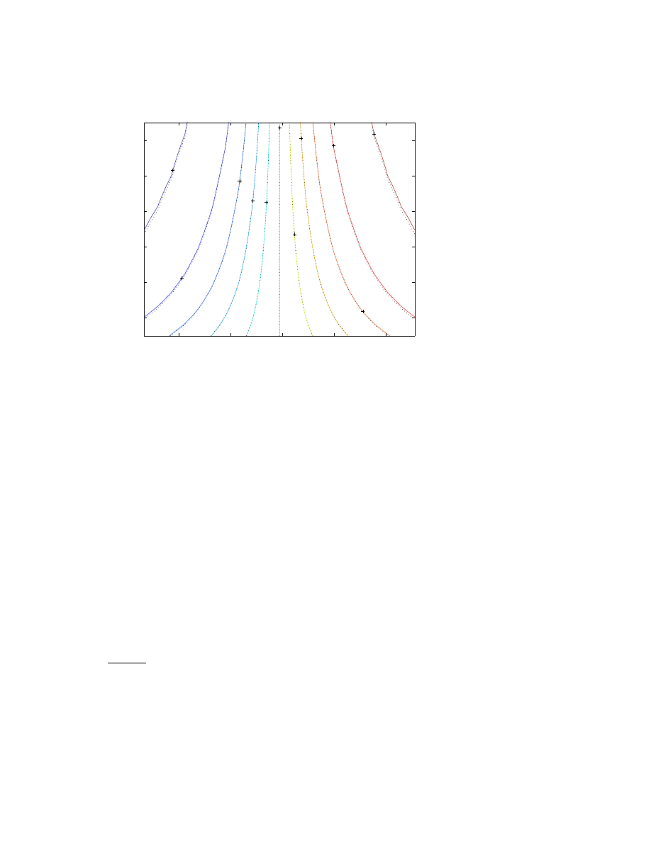
Exponential Asymptotics
51
1.9
2
2.1
2.2
2.3
4
6
8
10
12
14
0.01
0.1
0.2
0.3 0.4
0.5
0.6
0.7
0.8
0.9
0.99
θ
/
π
|z|
Stokes multiplier, approximated by terminant
Figure 11. Solid: contours of the integral approximating the Stokes multiplier for
the Airy function. Dashed: contours of the error function approximation to this
integral. The solid and dashed contours are almost indistinguishable, which is a
graphical demonstration that the steepest descent approximation to the integral is
very accurate.
order) in terms of the Airy function Ai. This is matched to standard
WKB approximations which describe the solution everywhere else.
For “above-the-barrier” scattering, however, what is one to do?
Pokrovskii and Khalatnikov [262] had a flash of insight: actually, there
are turning points, but only for complex x. In the vicinity of these
off-the-real-axis turning points, the reflected wave is not small, so the
usual connection formulas apply with only minor modifications. The
amplitude of the reflected wave decays exponentially as
=(x) → 0 so
that, on the real x-axis, the reflection coefficient is exponentially small
in 1/², the inverse width of the barrier.
2
Kruskal and Segur [171, 172, 278] showed that matching expan-
sions at off-the-real-axis critical points was a powerful method for non-
linear problems, too. Their first application resolved a forty year old
conundrum in the formation of multi-branched fingers (“dendrites”)
on a solid-liquid interface. The unique length scale observed in the
2
Pokrovskii relates an amusing story: when he presented his work to the Nobel
laureate, Lev Landau, the great man thought he and Khalatnikov were crazy! He
eventually changed his mind.[261]
ActaApplFINAL_OP92.tex; 21/08/2000; 16:16; no v.; p.51

52
John P. Boyd
laboratory is imposed by surface tension. However, the scale-selecting
effect lies “beyond all orders” in a power series expansion in the surface
tension parameter. Their method, which we shall henceforth call the
“PKKS” [Pokrovskii-Khalatnikov-Kruskal-Segur] scheme for short, has
been widely used for weakly nonlocal solitary waves (Table III).
To illustrate the PKKS method, we shall apply it to the linear prob-
lem:
u
xx
+ u = f (²x)
(91)
where f (x) will be restricted to functions that (i) decay exponential-
ly as
| x |→ ∞ on and near the real axis and (ii) have a complex
conjugate pair of double poles at x =
±i as the singularities nearest
the real axis and (iii) are symmetric with respect to x = 0, that is,
f (x) = f (
−x). This seems like a rather special and restrictive prob-
lem. However, as Dingle observed long ago, every simple example is a
master-key to an entire class of problems, as we shall show. This linear
problem is identical to that solved earlier, Eq.(26), except for the sign
of the undifferentiated term in u.
We shall impose the boundary condition that
u
∼ α sin(|x|) as |x| → ∞
(92)
for some constant α which will be determined as part of the solution.
This excludes the homogeneous solutions sin(x) and cos(x) so as to
yield a unique solution. (Note the absolute value bars inside the argu-
ment of the sine function in the boundary condition.)
The PKKS method has the following steps:
1. Identify the singularities or critical points which are nearest the
real x-axis
2. Define an “inner” problem, that is, a perturbative scheme which
is valid in the neighborhood of one of these critical points, using a
complex coordinate y whose origin is at the critical point.
3. Asymptotically solve the “inner” problem as
| y |→ ∞, that is,
compute the “outer limit of the inner solution”.
4. Sum the divergent outer limit of the inner problem by Borel sum-
mation or otherwise determine the connection formula, that is, the
magnitude and phase of the discontinuity along the Stokes line
radiating from the critical point to the real x-axis
5. Match the outer limit of the inner solution to the inner limit of the
outer expansion
ActaApplFINAL_OP92.tex; 21/08/2000; 16:16; no v.; p.52
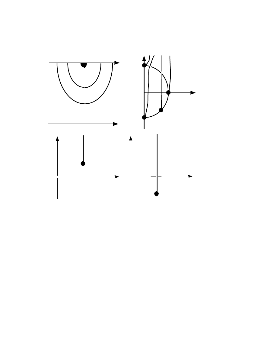
Exponential Asymptotics
53
AAAAAAAAAA
AAAAAAAAAA
AAAAAAAAAA
AAAAAAAAAA
AAAAAAAAAA
AAAAAAAAAA
AAAAAAAAAA
AAAAAAAAAA
AAAAAAAAAA
AAAAAAAAAA
AAAAAAAAAA
AAAAAAAAAA
AAAAAAAAAA
AAAAAAAAAA
AAAAAAAAAA
AAAAAAAAAA
AAAAAAAAAA
AAAAAAAAAA
AAAA
AAAA
AAAA
AAAA
AAAA
AAAA
AAAAA
AAAAA
AAAAA
AAAAA
AAAAA
AAAAA
Real x-axis
Real y-axis
AAA
AAA
AAA
AAA
AAA
AAA
AAA
AAA
Inner
Matching
Outer
arg(y)=0
arg(y)=
-
π
Im(t)
AA
AA
AA
AA
A
A
A
A
A
A
AA
AA
AA
AA
AA
AA
AA
AA
AA
AA
A
A
A
A
A
A
A
A
A
arg(y)=
-
π/2
arg(y)=
-(3/4)
π
Re(t)
Im(t)
Re(t)
Im(t)
Re(t)
AAAA
AA
AA
A
A
A
A
A
A
AA
AA
A
A
A
A
AA
AAA
AA
A
AAAAAAAA
A
A
A
A
AA
AA
AA
AA
AA
AA
AA
AA
arg(y)=
-(1/4)
π
arg(y)=
-(3/4)
π
Figure 12. (a) [Upper left corner] Schematic of complex y-plane where y is the
shifted coordinate. (The real axis in the original coordinate x is the arrow at the
bottom.) The location of the double pole (at y = 0) is the large solid dot at top.
The “matching” region, shaped like a half annulus, is where both the inner and
outer solutions are valid, allowing them to be matched. (b) [Upper right corner] The
complex t-plane where t is the integration variable for the Borel-logarithm function,
Bo(y). The four large black discs show the location of the logarithmic singularity
of the integrand for four different values of arg(y). The branch cut (cross-hatched
lines) goes to i
∞ for all cases. As arg(y) increases, the location of the branch cut
rotates clockwise. For arg(y) <
−π/2, the branch cut crosses the real t-axis as shown
in the lower right half diagram. (c) [Bottom half of the figure]. Both left and right
panels illustrate the path of integration in the complex t-plane (heavy, patterned
curves) and the branch cuts for the logarithm of the integrand (cross-hatched lines).
The left diagram shows the situation when arg(y) =
−π/4, or any other point such
that the branch point is in the upper half of the t-plane: the branch cut does not
cross the real axis. When arg(y) <
−π/2 [right, bottom diagram], the integration
path must be deformed below the real t-axis to avoid crossing the branch cut. The
integration around the branch cut adds an additional contribution.
ActaApplFINAL_OP92.tex; 21/08/2000; 16:16; no v.; p.53

54
John P. Boyd
6. Continue the matched outer expansion back to the real x-axis to
compute the (exponentially small) magnitude of the Stokes jump
for real x.
The domains of the “inner” and ”outer” regions are illustrated in
Fig. 12.
Step one has already been accomplished by the specification of the
problem: the relevant critical points are the double poles of f (²x) at
x =
±i/² where the change of variable from x to ²x has reduced the
residues to 1/²
2
. The shifted coordinate (for matching in the upper
half-plane) is
y
≡ x − i/²
(93)
Step two pivots on the observation that in the vicinity of its double
pole, it is a legitimate approximation to replace f (²x) by the singular
term only, even though this is a poor approximation everywhere except
near the pole. The inner problem is then
U
yy
+ U = 1/y
2
;
U
≡ ²
2
u
(94)
Step three, computing an outer expansion for the inner problem, is
obtained by an inverse power series in y:
U (y)
∼
∞
X
j=1
(
−1)
j+1
(2j
− 1)!
y
2j
(95)
For the inner problem to be sensible,
| y |<< 1/². For the inverse
power series to be an accurate approximation to the inner solution, we
must have
| y |>> 1. It follows that the inverse power series is a good
approximation only in the annulus
1 <<
| y |<< 1/²
(96)
It is fair to dub this annulus the “matching region” because it will turn
out that the inner limit of the outer expansion will also be legitimate in
this annulus. However, “annulus” is a slightly misleading label because
Eq.(96) ignores Stokes phenomenon, which will limit the validity of
Eq.(95) to a sector of the annulus.
To sort out Stokes phenomenon, it is helpful to sum the divergent
series by Borel summation. For this simple case, the Borel transform
can be written in closed form to give, without approximation,
U (y) = (1/2)Bo(y);
Bo(y)
≡
Z
∞
0
exp(
−t) log{1 + t
2
/y
2
} dt
(97)
ActaApplFINAL_OP92.tex; 21/08/2000; 16:16; no v.; p.54

Exponential Asymptotics
55
The integrand is logarithmically singular at t =
±iy. As the argument
of y varies from 0 to
−π, that is, through a semicircle in the lower half
of the y-plane, the singularity initially in the upper half of the t-plane
rotates clockwise through a semicircle in the right half of the t-plane to
exchange places with the other branch point. As arg(y) passes through
−π/2, that is, through the negative imaginary y − axis, the branch
points of the “Borel-logarithm” function Bo(y) are forced to cross the
real t-axis. To avoid discontinuously redefining the branch points of the
logarithm in the integrand, the path of integration must be deformed
to pass below the real t-axis (in the right half t-plane). This gives an
extra contribution which is the Stokes jump for this function with the
negative imaginary y-axis as the Stokes line. One finds
Bo(y)
− Bo(−y) = 2πi exp(−iy)
(98)
The positive and negative real y-axis are the anti-Stokes lines for Bo(y).
The outer expansion is the same as the multiple scales series for
Eq.(26) except for alternating signs; The final result on the real x-axis
is
u(x)
∼
−
π
²
2
exp
¡
−
x
s
²
¢
+
P
∞
j=0
(
−1)
j
²
2j d
2j
f
dX
2j
,
x
≥ 0
π
²
2
exp
¡
−
x
s
²
¢
+
P
∞
j=0
(
−1)
j
²
2j d
2j
f
dX
2j
,
x < 0
(99)
where the outer expansion has been written in terms of derivatives of
f (²x)
≡ f(X) with respect to the “slow” variable X ≡ ²x to explicitly,
rather than implicitly, display the dependence of the j-th term on ²
2j
.
Extrapolating back to the real axis reduces the magnitude of the
jump by exp(
−x
s
/²) = exp(
−1/²) where x
s
/² is simply the distance of
the singularity from the real x-axis. Note that the exponential depen-
dence on ² is controlled entirely by x
s
/²; the strength of the residue
and the type of singularity (simple pole, double pole or logarithm)
only alters factors that vary as powers of ² or slower.
We chose this particular example because the theory of Pomeau,
Ramani and Grammaticos [263] for the Fifth-Order Korteweg-deVries
equation, later extended to higher order by Grimshaw and Joshi [134],
is very similar. In particular, the dominant singularities – in their case,
of the lowest order approximation to the solitary wave – are also dou-
ble poles on the imaginary axis. It is also true that the outer limit
of the inner solution is the Borel-logarithm function, Bo(y) [to lowest
order]. Consequently, the lowest order theory for this nonlinear eigen-
value problem is almost identical to that for this linear, inhomogeneous
problem. The major difference is that the nonlinearity multiplies Bo(y)
ActaApplFINAL_OP92.tex; 21/08/2000; 16:16; no v.; p.55

56
John P. Boyd
by a constant which can only be determined numerically by extrapo-
lating the recurrence relation. The early terms of the series in inverse
powers of y in the matching region is strongly affected by the nonlinear-
ity, but the coefficients asymptote to those of Bo(y), another triumph
of Dingle’s maxim: Always look at the late terms where a whole class
of problems asymptote to the same, common form.
As noted by a reviewer, the integral for Bo can be integrated by
parts to express it as the sum of two Dingle terminants, and the connec-
tion formulae can then be evaluated through residues. This alternative
derivation of the same answer emphasizes the remarkable universality
of hyperasymptotics; again and again, one keeps falling over the same
small set of terminants.
Table III records many successes for the PKKS method, but it is a
curious success. It is a general truth that the exponential dependence
on ² is controlled entirely by x
s
, the distance from the relevant singu-
larities or critical points to the real axis. This is usually almost trivial
to determine. Roughly 90% of the work of the PKKS method is in
determining the “prefactor”, that is, the product of a constant times
algebraic factors of ², such as logarithms and powers, which multiplies
the exponential. Not only is the determination of the prefactor (com-
paratively) arduous, but the final step of determining the overall multi-
plicative constant must always be done numerically. Pomeau, Ramani
and Grammaticos and later workers such as Akylas and Yang [5] and
Boyd [68] have simplified the numerical bit to extrapolating a sequence
derived from a recurrence, a task much easier than directly solving a
differential equation. However, the fact that the PKKS method is an
analytical method that is not entirely analytic gives much ground to
alternatives such as spectral methods which are discussed later.
15. Snares and Worries: Remote but Dominant Saddle
Points, Ghosts, Interval-Extension and Sensitivity
“There are, so to speak, in the mathematical country, precipices and
pit-shafts down which it would be possible to fall, but that need not
deter us from walking about.”
— Lewis F. Richardson (1925)
More subtle perils in deriving even the lowest order correctly also
lurk. Balian, Parisi and Voros [11] describe an integral where the con-
vergence is controlled by a saddle point at t = 2, but the error is
dominated by the exponentially larger contributions of another saddle
ActaApplFINAL_OP92.tex; 21/08/2000; 16:16; no v.; p.56

Exponential Asymptotics
57
point at t = 3. Their function is
I(z)
≡
Z
∞
−∞
exp
³
−z
n
36t
2
− 20t
3
+ 3t
4
o´
dt
(100)
For large z, the integrand is steeply peaked about the dominant saddle
point at t = 0 (Fig. 13). The contributions of the other two saddle
points will be proportional to the integrand evaluated at these saddle
points:
exp(
−zφ(t = 2)) = exp(−32z), exp(−zφ(t = 3)) = exp(−27z) (101)
Because the saddle point at t = 2 controls convergence, the smallest
term in the asymptotic series for a given z will be O(exp(
−32z)), so we
would expect this to be the magnitude of the error in the optimally-
truncated series in inverse powers of z. In reality, the superasymptotic
error is dominated by the contribution of the saddle point at t = 3,
which is O(exp(
−27z)) and therefore larger than the smallest term in
the optimally- truncated series by O(exp(5z)).
One of the charms of resurgence theory is that during the early
stages, all saddle points are treated equally. This “saddle point democ-
racy” is valuable in detecting such pathologies, and correctly retain-
ing the contributions of all the important saddle points. Still, if the
asymptotic series is derived not from an integral but directly from a
differential equation so that no information is available but the coeffi-
cients of the series, it would be easy to be fooled, and assume that the
magnitude of the smallest retained term was a genuine estimate of the
superasymptotic error.
Fortunately, it appears that this is rare in practice. The applied
mathematical landscape is littered with deep sinkholes which fortu-
nately have an area of measure zero. The Balian-Parisi-Voros example
was contrived by its authors rather than derived from a real application.
However, related difficulties are not contrived.
For the so-called φ
4
breather problem [278, 58], the convergence of
the divergent series is controlled by the constant in the Fourier series
with an expected minimum error of O(exp(
−
√
2π/(2²))). However, the
far field radiation has a magnitude α which has been shown to be
O(exp(
−
√
6π/(2²))). Thus, after the ²-power series has been truncated
at optimal order and subtracted from the solution, the correction is
still exponentially large in ² relative to the weakly nonlocal radiation.
Complex-plane matched asymptotics is not inconvenienced [278], but
the hyperasymptotic method of Boyd [67] would likely fail.
Another danger is illustrated by the function
f (²)
≡ S(²) + exp(−(1/2)/²)
(102)
ActaApplFINAL_OP92.tex; 21/08/2000; 16:16; no v.; p.57
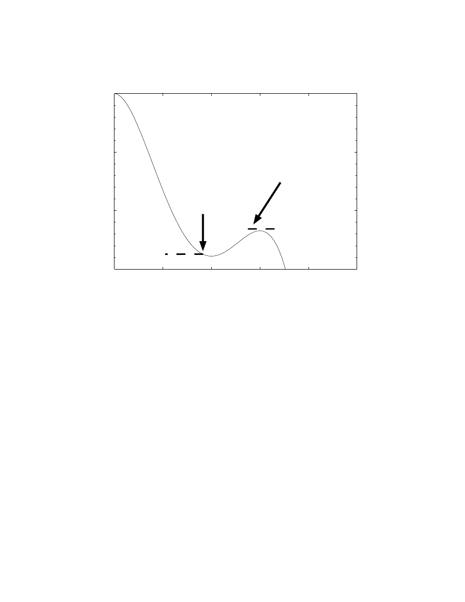
58
John P. Boyd
0
1
2
3
4
5
10
-15
10
-10
10
-5
10
0
t
exp(- phi(t))
Balian-Parisi-Voros Example
Minimum
Error
Smallest
Term
Convergence-
Controlling
Saddle Pt.
Error-
Determining
Saddle Pt.
Figure 13. The integrand of the example of Balian, Parisi and Voros: exp(
−φ). The
dominant saddle point is at t = 0. The secondary peak (saddle point) at t = 2
controls the asymptotic form of the coefficients of the asymptotic series; because
of it, the series for dt/dw converges only for
| w |≤| w(t = 2) | . However, the
contribution of the more distant saddle point at t = 3 dominates the error. The
terms of the power series in 1/z reach a minimum at roughly exp(
−zφ(t = 2)), but
the error in the optimally–truncated series is exponentially large compared to this
minimum term, being roughly exp(
−zφ(t = 3))
where S(²) is the Stieltjes function. The asymptotic expansion for this
function is the same as for the Stieljes function; because exp(
−(1/2)/²)
and all its derivatives vanish as ²
→ ∞, this function makes no contri-
bution to the divergent power series of f (²). It follows that if we manip-
ulate the power series in the usual way, we arrive at a superasymptot-
ic approximation which, from the size of the smallest term, has an
error apparently of O(exp(
−1/²). Adding a Dingle terminant gives a
hyperasymptotic approximation of even smaller error — more fool we!
Because we are approximating f (²) (at best!) by the Stieltjes function
S(²), the error is actually the magnitude of the second term — exponen-
tially larger than exp(
−1/²). Quick to defend the honor of hyperasymp-
totics, a reviewer argued that this is merely a problem of definition. An
ActaApplFINAL_OP92.tex; 21/08/2000; 16:16; no v.; p.58

Exponential Asymptotics
59
engineer’s answer: a wrong answer is never just a matter of definition,
but rather a good reason to lie awake at night, and retain a lawyer.
Weakly nonlocal solitary waves are a nontrivial example of phenom-
ena with exponentially small “ghosts”: the solitons can be expanded
in non-trivial power series in ², but the amplitude α of the sinusoidal
oscillations of the soliton for large
| x | is proportional to exp(−µ/²)
for some constant µ. The terms in the power series are, in the sim-
plest cases, powers of sech(²x) and therefore each term individually
decays exponentially fast as
| x |→ ∞. It follows that standard accel-
eration methods must fail because reweighting the terms of the power
series still gives nothing at infinity, and thus misses the far field oscilla-
tions completely. The Dingle terminants method, which is based on the
asymptotics of the power series coefficients, has never been successfully
applied to this sort of problem either.
Fortunately, the PKKS method, spectral algorithms, the spectral
space asymptotics of Akylas and Yang [5, 325, 326] and the hyper-
asymptotic scheme of Boyd [68] all work well for nonlocal solitary
waves. Nevertheless, the failure of some alternative schemes for this
class of problems because the quantity of interest is invisible to the
power series are vivid reminders of the truism: Fear and caution are
healthy character traits in an applied mathematician!
Another pitfall is extending the interval of integration to infinity.
For example, the Bessel function I
0
(z) has a representation that is an
integral over a finite interval:
I
0
(z)
≡
1
2π
exp(z)
Z
π
−π
exp (z[cos(t)
− 1]) dt
(103)
Without approximation, we can make the change of variable 2w
2
=
1
− cos(t) to obtain
I
0
(z) =
1
π
exp(z)
Z
1
−1
exp
³
−2zw
2
´
1
(1
− w
2
)
1/2
dw
(104)
The usual procedure is to expand the 1/
√
1
− w
2
as a power series,
extend the interval of integration to w
∈ [−∞, ∞], and integrate term-
by-term to obtain the expansion given in most references:
I
0
(z)
∼ exp (z)
µ
1
2πz
¶
1/2
½
1 +
1
8
z
−1
+
9
128
z
−2
+ . . .
¾
(105)
The sole reason for the divergence of this series is the extension of
the interval. If we expand and integrate term-by-term on the original
interval w
∈ [−1, 1], the result is a series that converges – albeit rather
ActaApplFINAL_OP92.tex; 21/08/2000; 16:16; no v.; p.59

60
John P. Boyd
slowly because the radius of convergence of the power series under the
integrand is just equal to the limit of integration so that the terms
of the integrated series decrease only as O(1/j
3/2
) for the coefficient
of 1/z
j
in the series. Why, then, is interval-extension so ubiquitous in
asymptotics?
The answer is two-fold. First, the terms of the series are greatly
simplified at the price of divergence. The one-term approximation is
simplified from an error function to a Gaussian, for example, and the
higher order terms of the convergent series become more and more
complicated; to the same order as above, the convergent series is
I
0
(z) =
1
π
exp(z)
{
r
π
2 z
erf
³
√
2 z
´
+
r
π
2
erf
³
√
2 z
´
8 z
3/2
−
1
4
exp(
−2 z)
z
+
3
256 z
5/2
³
−12
√
z exp(
−2 z) − 16 z
3/2
exp(
−2z) + 3
√
2π erf
³
√
2 z
´´
}
(106)
The second reason is that because the convergent series is only slowly
convergent, it is far from obvious that the error can be reduced much
below the superasymptotic limit unless one uses a very large number
of terms in the convergent series. It is more practical to restrict z to
such large values that the superasymptotic approximation is acceptably
accurate, and use the ordinary Taylor series for smaller z.
Another snare is that exponentially small quantities, when paired
with a non-trivial powers, are often extremely sensitive to small changes
in parameters. For example, the solution of the differential equation
equation
u
xx
+ u = sech(² x) + ²
2n
−1
d(²) (2n
− 1)! sech
2n
(² x)
(107)
asymptotes to a sinusoidal oscillation with an amplitude α(²), which is
an exponential function of 1/². One can choose an O(1) function d(²)
such that α(²) is zero. And yet if ² = 1/10 and n = 3, the second term
in the forcing is more than a thousand times smaller than the first!
The moral is that in physical applications, it is not sufficient merely
to calculate the exponentially small effects. One must also look at how
small perturbations of the idealized problem might drastically change
the exponentially small contributions.
ActaApplFINAL_OP92.tex; 21/08/2000; 16:16; no v.; p.60

Exponential Asymptotics
61
16. Asymptotics as Hyperasymptotics for Chebyshev,
Fourier and Other Spectral Methods
One important but neglected area of asymptotics is numerical analysis,
specifically, approximations to the error as a function of the grid spac-
ing h (or other discretization parameters). For the familiar numerical
integration scheme known as the trapezoidal rule, for example, which
is defined by
I
≡
Z
1
0
g(y)dy
∼ T ≡
1
M
{
1
2
g(0) +
1
2
g(1) +
M
−1
X
j=1
g
µ
j
M
¶
}
(108)
where the grid spacing h is
h
≡ 1 /M,
(109)
the Euler-Maclaurin sum formula gives the following asymptotic series
for the error [143]
I
− T ∼ −
N
X
j=1
h
2j
B
2j
(2j)!
n
g
(2j
−1)
(1)
− g
(2j
−1)
(0)
o
+ E
N
(110)
where the B
2j
are the Bernoulli numbers and the error is
E
N
≡ −h
2N +2
B
2N +2
(2N + 2)!
g
(2N +2)
(ξ)
(111)
with ξ a point somewhere on the interval [0, 1].
Elementary numerical analysis courses usually stop with the obser-
vation that since the leading term is proportional to h
2
, the trapezoidal
rule is a “second order” method. However, the series in powers of h con-
tains hidden depths. First, if the rule is applied twice with different grid
spacings h and 2h, one can take a weighted difference of T(h) and T(2h)
such that the quadratic terms cancel in (110):
4 T (h)
− T (2h)
3
∼ I + O(h
4
)
(112)
This improved integration scheme is “Simpson’s Rule”. This strategy
can be iterated to obtain methods of progressively higher accuracy and
complexity not only for quadrature schemes, but for finite difference
approximations, too. The generalization to arbitrary order is known as
“Richardson extrapolation” [270, 271] or to use his own term, “deferred
approach to the limit”.
ActaApplFINAL_OP92.tex; 21/08/2000; 16:16; no v.; p.61

62
John P. Boyd
Second, if the integrand g(x) is a periodic function, then g
2j
−1
(1) =
g
2j
−1
(0) to all orders j, and the error expansion reduces to the trivial
one:
I
∼ T + 0h
2
+ 0h
4
+ 0h
6
+ . . .
(113)
Within the Poincar´
e asymptotic framework, this suggests the trape-
zoidal rule is exact for all periodic functions — Wrong!
The integral of g(x) is proportional to the constant in the Fourier
expansion of g(x); the usual formula for the error in computing Fourier
coefficients through the trapezoidal rule [55] gives
I
− T = −
∞
X
j=1
a
jN
(114)
where the
{a
j
} are the exact Fourier cosine coefficients of g(x),i. e.,
a
j
≡ 2
Z
1
0
g(x) cos (2π j[x
− 1/2]) dx
(115)
(Note that in (114), the degree of the Fourier coefficient is the product
of the sum variable j with N so that only every N -th coefficient appears
in the error series.) For a periodic function, it is known that
a
j
∼ ν(j) exp(−2πµj)
(116)
where µ is the absolute value of that singularity in the complex x-
plane which is closest to the real axis and where the prefactor ν is an
algebraic rather than exponential function of j which depends on the
type of singularity (simple pole, logarithm, etc.). Inserting this into
Eq. (114) gives the correct conclusion that for periodic functions, free
of singularity for real x, the error in the trapezoidal rule is
I
− T ∼ ν exp(−2πµ/h).
(117)
In other words, the error lies beyond all orders in powers of the grid
spacing h.
Presumably such exponential dependence on 1/h lurks in the Euler-
Maclaurin series even for non-periodic functions. We can confirm this
suspicion by considering a particular case: a function g(x) whose sin-
gularity nearest the interval x
∈ [0, 1] is a simple pole of unit residue at
x =
−σ. In the limit that the order j → ∞, the (2j − 1)-st deriva-
tive will be more and more dominated by this singularity. (Recall
that the convergence of the power series in x about the origin has
a radius of convergence σ controlled by this nearest singularity, and
that the coefficients of the power series are the derivatives of g(x) at
ActaApplFINAL_OP92.tex; 21/08/2000; 16:16; no v.; p.62

Exponential Asymptotics
63
the origin.) Using the known asymptotics of the Bernoulli numbers,
B
2j
∼ (−1)
j
−1
(2j)!/(2
2j
−1
π
2j
), we find
h
2j
B
2j
(2j)!
n
g
(2j
−1)
(1)
− g
(2j
−1)
(0)
o
∼ 2(−1)
j
h
2j
2
2j
π
2j
σ
2j
j!,
j
→ ∞
(118)
This implies one can obtain an improved trapezoidal rule by subtracting
the leading term of the hyperasymptotic approximation to the error in
the ordinary trapezoidal rule. This is obtained by optimally-truncating
the Euler-Maclaurin series and approximating the error by a Dingle
terminant:
E
N
∼ Λ
N
Ã
h
2
4π
2
σ
2
!
(119)
One important implication of the factorial divergence of the Euler-
Maclaurin series is that it shows that Richardson extrapolation will
diverge, too, if applied to arbitrarily high order for fixed h. Romberg
integration, which is a popular and robust algorithm for numerical
integration, does in fact employ Richardson extrapolation of arbitrary
order. However, at each stage, the grid spacing h is halved. In the lim-
it that 1/h and the order of Richardson extrapolation simultaneously
tend to infinity, the quadrature scheme converges.
Lyness and Ninham [190] noted this exponential dependence on 1/h
in quadrature errors nearly thirty years ago. Lyness has emphasized
that the Euler-MacLaurin series for the trapezoidal rule is closely relat-
ed to a general formula for the coefficients of a Fourier series. His
“FCAE” [Fourier Coefficient Asymptotic Expansion] takes the form
[188, 189]
a
n
=
M
X
k=1
(
−1)
n+k
−1
g
2k
−1
(1)
− g
2k
−1
(0)
(2πn)
2k
(120)
+
(
−1)
M +1
(2πn)
2M +1
Z
1
0
g
(2M +1)
(x) sin(2π n[x
− 1/2] )dx
plus a similar series for the sine coefficients. It is derived by integration-
by-parts. As noted by Lyness, it is usually divergent.
As explained in the books by Boyd [55] and Canuto et al. [91], spec-
tral methods usually employ a basis set so that the error is exponential-
ly small in 1/h or equivalently, in the number of degrees of freedom M .
Fourier series, for example, are restricted to periodic functions. Cheby-
shev polynomials give exponential convergence even for non-periodic
functions, provided only that f(x) is free of singularities on x
∈ [−1, 1].
These polynomials are defined by T
n
(cos[θ])
≡ cos(n θ) so that the
ActaApplFINAL_OP92.tex; 21/08/2000; 16:16; no v.; p.63

64
John P. Boyd
expansion of f (x) as a Chebyshev series is identical, under this change
of variable, with the Fourier expansion of f (cos(θ)). The transformed
function is always periodic in θ, so the error in truncating a Chebyshev
series after M terms decreases exponentially fast with M . For Cheby-
shev and Fourier spectral methods, the power series in h is always the
trivial one with zero coefficients.
It follows that all asymptotic approximations to Fourier, Chebyshev,
and other spectral coefficients for large M are implicitly hyperasymp-
totic (Table V). One might object that this catalogue of asymptotics for
orthogonal series is out of place here because it is “beyond all orders”
[in h] only because the coefficients of all powers of h are zero. The
main tools for the work of Elliott, Miller, Luke, Weideman and Boyd
were steepest descents and the calculus of residues — no explicit use
of hyperasymptotic thinking at all.
Nevertheless, Table V makes several important points. First, much
of hyperasympotics is steepest descent and the calculus of residues. In
discussing the Stieltjes function earlier, for example, we noted that one
could go beyond the superasympotic approximation by applying steep-
est descent to the error integral of the optimally-truncated ² power
series. Similarly, the heart of the PKKS technique of matched asymp-
totic expansions in the complex plane is the notion that the singular-
ities or other critical points closest to the real axis control the hyper-
asymptotic behavior. The asymptotic behavior of the coefficients of
orthogonal expansions is likewise controlled by complex singularities.
In both cases, the constant q inside the exponential factor, exp(
−q/²)
or exp(
−q/h), is simply the distance from the dominant singularity to
the real x-axis.
3
Second, an important hyperasymptotic strategy is to isolate the
exponentially small contributions. For the large degree behavior of
Chebyshev and Fourier coefficients, this isolation is a free gift, the result
of choosing the sensible spectral basis — Chebyshev or Legendre poly-
nomials for non-periodic problems, spherical harmonics for problems
on the surface of a sphere and so on. For less trivial problems, the key
to isolation is to subtract an optimally truncated asymptotic expansion.
This is the justification for applying steepest descent to the error inte-
gral for Stieltjes function, for applying Euler’s method or other sum
acceleration scheme, for Dingle’s universal terminants and for Berry’s
smoothing of Stokes phenomenon. The difference between a quantity
and its superasymptotic approximation is as trivially isolated as the
3
For Chebyshev series, “distance from the real axis” means distance in the trans-
formed coordinate θ, the argument of the equivalent Fourier series, rather than the
argument of the Chebyshev polynomials, x = cos(θ).
ActaApplFINAL_OP92.tex; 21/08/2000; 16:16; no v.; p.64

Exponential Asymptotics
65
spectral coefficients of a Fourier series, for which the superasymptotic
approximation is zero.
Third, the asymptotics of spectral series and other numerical pro-
cesses is a relatively under-cultivated area. Can the ideas reviewed here
lead to optimal order Richardson extrapolation for numerical quadra-
ture, various classes of differential equations, and so on?
Fourth, there have been some limited but important excursions
beyond conventional asymptotics in the analysis of the convergence
of spectral series. For example, Boyd’s 1982 article on the optimization
of Chebyshev methods on an unbounded domain notes that there are
two different species of contributions to the asymptotic spectral coef-
ficients: (i) saddle point contributions that depend on how rapidly the
function f (x) being expanded decays as
| x |→ ∞ and (ii) contribu-
tions from the poles and other singularities of f (x). In the limit that
the degree n of the rational Chebyshev coefficient tends to infinity for
fixed value of the “map parameter” L, one type of contribution will be
exponentially large compared to the other, and it is inconsistent (in the
Poincar´e sense of asymptotics) to retain the other. Boyd points out that
to optimize numerical efficiency, one should allow L to vary with the
truncation N of the Chebyshev series. Convergence is optimized when
N and L simultaneously tend to infinity in a certain way so that both
the pole and saddle point contributions are of equal order. This sort
of analysis does not explicitly use exponentially-improved asymptotics
of the Dingle-Berry-Olver sort. Nevertheless, hyperasymptotic thinking
— considering the role of terms that at first glance are exponentially
small compared to the dominant terms — is absolutely essential to this
kind of numerical optimization.
A few other interesting studies of the role of exponential smallness
in numerical analysis have already been made. For example, the usual
second order differential equation for the nonlinear pendulum, q
tt
+
sin(q) = 0, can be written as the equivalent system
p
t
= sin(q),
q
t
= p
(121)
where q is the angle of deflection of the pendulum with q = 0 when the
pendulum is standing (unstably) on its head and p is the momentum.
Hakim and Mallick [136] show that when the first equation is discretized
by a forward difference and the second equation by a backward differ-
ence, the system (121) becomes what in dynamical systems theory, with
a slight change in notation, is called the “standard mapping”:
p
n+1
= p
n
+ τ sin(q
n
),
q
n+1
= q
n
+ τ p
n+1
(122)
The usual numerical analysis description begins and ends with the
statement that this algorithm is second order accurate, that is, has
ActaApplFINAL_OP92.tex; 21/08/2000; 16:16; no v.; p.65
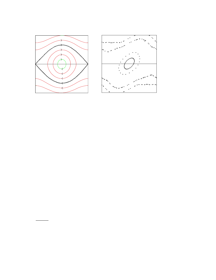
66
John P. Boyd
AAAAAAAAAAAAAA
AAAAAAAAAAAAAA
AAAAAAAAAAAAAA
AAAAAAAAAAAAAA
AAAAAAAAAAAAAA
AAAAAAAAAAAAAA
AAAAAAAAAAAAAA
AAAAAAAAAAAAAA
AAAAAAAAAAAAAA
AAAAAAAAAAAAAA
AAAAAAAAAAAAAA
AAAAAAAAAAAAAA
AAAAAAAAAAAAAA
AAAAAAAAAAAAAA
AAAAAAAAAAAAAA
AAAAAAAAAAAAAA
AAAAAAAAAAAAAA
AAAAAAAAAAAAAA
q
p
-3
0
3
0
π
2 π
q
p
-3
0
3
0
π
2 π
Figure 14. Phase plane for the nonlinear pendulum. Left panel: trajectories for the
exact solution. Right panel: trajectories when the differential equation is integrated
by a finite difference scheme, i. e, the “standard mapping”, with τ = 1. The cross-
hatched area is the region spanned by a single chaotic trajectory. To avoid printer
overload, the individual iterates were erased and replaced by a uniform texture.
an error which is proportional to τ
2
.
4
Hakim and Mallick point out
that there are also changes which are exponentially small in 1/τ — and
qualitatively different from the effects of finite differencing which are
proportional to powers of the timestep.
These changes are easiest to explain by examining the trajectories
of the differential equation and the difference system in the phase plane
(Fig. 14). The nonlinear pendulum is an exactly integrable system, and
all trajectories are periodic. The closed curves in the phase plane rep-
resent side-to-side, small amplitude oscillations of the pendulum. The
open curves at top and bottom show trajectories in which the pendu-
lum swings through complete loops like a propeller. These two species of
trajectories are divided by the “separatrix”, which is a trajectory that
passes through q = 0, the unstable equilibrium, with zero momentum
p. The separatrix and trajectories near it are super-sensitive to per-
turbations because only a tiny additional amount of momentum will
suffice to push a large amplitude oscillation over the top and thereby
convert it into a propeller-like motion.
The difference system, alias “standard mapping”, is not integrable
and has chaotic solutions. When the time step τ is very small, however,
one would expect that in some sense the difference and differential sys-
4
The one-sided differences are only first order, but by eliminating p, one can
show that the system is equivalent to applying centered, 2d order differences to the
second order differential equation.
ActaApplFINAL_OP92.tex; 21/08/2000; 16:16; no v.; p.66

Exponential Asymptotics
67
tems would be close to one another. Indeed, trajectories away from the
separatrix are not drastically altered by the discretization; finite differ-
ences give a good approximation to these trajectories of the nonlinear
pendulum. The neighborhood of the separatrix, however, dissolves into
chaotic motion. The incoming and outgoing separatrices from the equi-
librium split with a splitting angle at the point where the separatrices
cross of approximately [136], [180]
φ
∼
3514.9
τ
3
exp
Ã
−
π
2
τ
!
(123)
The width of the region of chaos around the separatrices has a similar
exponential dependence.
The bland statement “the method is second order” or even a formal
expansion of the errors in powers of the timestep τ completely misses
the spawning of this region of chaos. Such exponentially small quali-
tative changes are perhaps less important in the real world, where the
original differential equation probably has regions of chaotic motion
anyway, than in the idealized world of exactly integrable systems such
as the nonlinear pendulum, the Korteweg-deVries equation and so on.
Still, it reiterates the theme that hyperasymptotics is important to
numerical analysis.
Hakim and Mallick observe that the discretized system can be inter-
preted in two ways: (i) a second order accurate approximation to the
pendulum system or (ii) a fourth order accurate approximation to
a nonlinear differential equation which is obtained by modifying the
pendulum equation by the addition of a higher derivative with a τ -
dependent coefficient. Although the second interpretation seems rather
artificial, it is also illuminating. Weakly nonlocal solitary waves and
hydrodynamic boundary layers arise in this same way through addi-
tion of a higher derivative with a coefficient proportional to the small
parameter. The result of such a singular perturbation is that the power
series in the small parameter is divergent, and there are effects which
depend on the exponential of the reciprocal of the small parameter.
17. Numerical Methods for Exponential Smallness or:
Poltergeist-Hunting by the Numbers, I: Chebyshev &
Fourier Spectral Methods
Because of the messiness of hyperasymptotic methods even for clas-
sical special functions and ordinary differential equations, numerical
algorithms are important both as checks and as alternatives to hyper-
asymptotics. The exponential dependence on 1/² for ² << 1 cries out
ActaApplFINAL_OP92.tex; 21/08/2000; 16:16; no v.; p.67

68
John P. Boyd
for numerical schemes whose error also falls exponentially with the
number of degrees of freedom M . Fortunately, Chebyshev and Fourier
spectral methods [55, 91] and also Pad´e approximants [9, 19] have this
property. In this section, we shall discuss spectral methods while Pad´e
algorithms are described in the following section.
However, when the unknown function f (²) has only a divergent pow-
er series and also has contributions that lie beyond all orders in ², both
the rate of convergence and (sometimes) the methodology are altered.
For example, when a function f (x) which is analytic on x
∈ [−1, 1] is
expanded in a Chebyshev series, the error decreases geometrically with
M, the truncation of the Chebyshev series. In other words, the error
E
M
= O(exp(
−µM)) as M → ∞.
When f (²) has only a divergent power series about ² = 0, the Cheby-
shev or other spectral series on an interval that includes this point
will lack geometric convergence. However, as long as the function is
infinitely differentiable (with bounded derivatives), it is easy to prove
by integration-by-parts that the error must decrease faster than any
finite power of M . “C
∞
” singularities do not defeat spectral methods,
but merely slow them down.
By using the method of steepest descents, one can often show that
the spectral coefficients for functions which are infinitely-differentiable-
but-nonananalytic on the expansion are “subgeometric with exponen-
tial index of convergence β”:
a
n
∼ ν(n) exp
³
−µn
β
´
(124)
where ν is a prefactor that varies algebraically rather than exponen-
tially with n. Elliott [124, 125] pioneered this method, but Miller [227]
first applied it to estimate Chebyshev coefficients for functions with
divergent power series about one endpoint of the expansion interval.
For example, denoting the coefficients of the corresponding divergent
power series by b
n
and the Chebyshev expansion interval by ²
∈ [0, γ],
Miller found for S(²) and
<((²)), respectively,
b
n
= (
−1)
n
n!
→ a
n
∼ (−1)
n
s
16π
3γ
exp
µ
1
3γ
¶
exp
Ã
−3
n
2/3
γ
1/3
!
(125)
b
n
= n!
→ a
n
∼ i (−1)
n
s
16π
3 γ
exp
µ
−
1
3γ
¶
×
(126)
exp
Ã
−i
3
3/2
2
n
2/3
γ
1/3
!
exp
Ã
−
3
2
n
2/3
γ
1/3
!
ActaApplFINAL_OP92.tex; 21/08/2000; 16:16; no v.; p.68
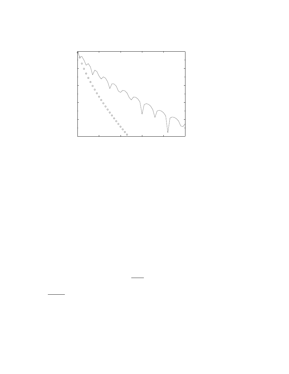
Exponential Asymptotics
69
0
10
20
30
40
50
10
-10
10
-8
10
-6
10
-4
10
-2
10
0
n
Figure 15. Chebyshev coefficients for the expansion on ²
∈ [0, 1] of the Stieltjes
function, S(²) [lower curve, circles] and
<[S(−²)] (upper curve, solid).
(One can show that the error in truncating an exponentially convergent
series after the N -th term is proportional to a
N
as explained in [55, 73].)
Note that even when the asymptotic series is monotonic, corresponding
to a principal value integral with a simple pole at t =
−1/² on the path
of integration, the Chebyshev series still happily converges. However,
roughly twice as many terms are needed to achieve the same accura-
cy for
<(S(−²)) as for S(²) (Fig. 15). Asymptotic approximations to
the subgeometrically decreasing Chebyshev coefficients for many other
special functions are given by Miller [227] and in the books by Luke
[187] and N´emeth [236].
5
It easy to derive asymptotic approximations for Chebyshev or other
spectral coefficients for specific functions, but few general results are
known. One such theorem applies to the class of Stieltjes functions,
which is defined to be the set of all functions that can be written in
the form
f (²)
≡
Z
∞
0
ρ(t)
1 + ²t
dt
(127)
5
It appears from his English-language monograph that N´
em´
eth independently
derived many asymptotic approximations in Hungarian-language articles in the mid-
60’s.
ActaApplFINAL_OP92.tex; 21/08/2000; 16:16; no v.; p.69

70
John P. Boyd
for some positive semi-definite weight function ρ(t) such that the moment
integrals
b
n
≡
Z
∞
0
t
n
ρ(t) dt
(128)
exist for all nonnegative integers n. (These moments are also the coef-
ficients of the power series expansion of f(²) about ² = 0.) W. G. C.
Boyd has developed a general theory for hyperasymptotics for Stieltjes
functions.
J. P. Boyd [49, 51] showed that if the power series coefficients diverge
as (n!)
r
or (rn)!, i. e.,
lim sup
n
→∞
log
| b
n
|
n log n
= r
(129)
then the Chebyshev coefficients satisfy the inequalities
2
r + 2
≥ lim sup
n
→∞
log
| (log | a
n
|) |
log n
≥ 1 −
r
2
(130)
Less precisely, the theorem implies that if the Chebyshev coefficients
are decreasing like O(exp(
−µn
β
)) for some constants µ and β, then β
must be smaller 2/(r + 2), implying subgeometric convergence for all
r > 0, i. e. all factorial divergence. However, the exponential index of
convergence β cannot be smaller than 1
− r/2.
The integration-by-parts theorem shows that even for r > 2, the
convergence of Chebyshev series is beyond all orders in 1/N . However,
it would be highly desirable to extend Boyd’s theorem to more general
classes of asymptotic functions, and perhaps sharpen it, too.
Berry [29] has shown that his error-function smoothing of Stokes
phenomenon applies even to several broad classes of functions whose
coefficients diverge faster than any factorial, so-called “superfactorial
asymptotics”. His numerical illustration is the function
BeS(²; A)
∼
∞
X
n=0
exp
Ã
n
2
A
!
²
n
≡
s
A
π
PV
Z
∞
−∞
exp
©
−A (t − (1/2) log(²))
2
ª
1
− exp(2 t)
dt(131)
where we have replaced his z by
−(1/2) log(²) so that the asymptotic
series is a conventional power series. Fig. 16 shows that Chebyshev poly-
nomials have no problem in providing a highly accurate approximation
even though the power series coefficients are blowing up like Gaussians
of n. Unfortunately, there are a hundred papers on the asymptotics and
ActaApplFINAL_OP92.tex; 21/08/2000; 16:16; no v.; p.70
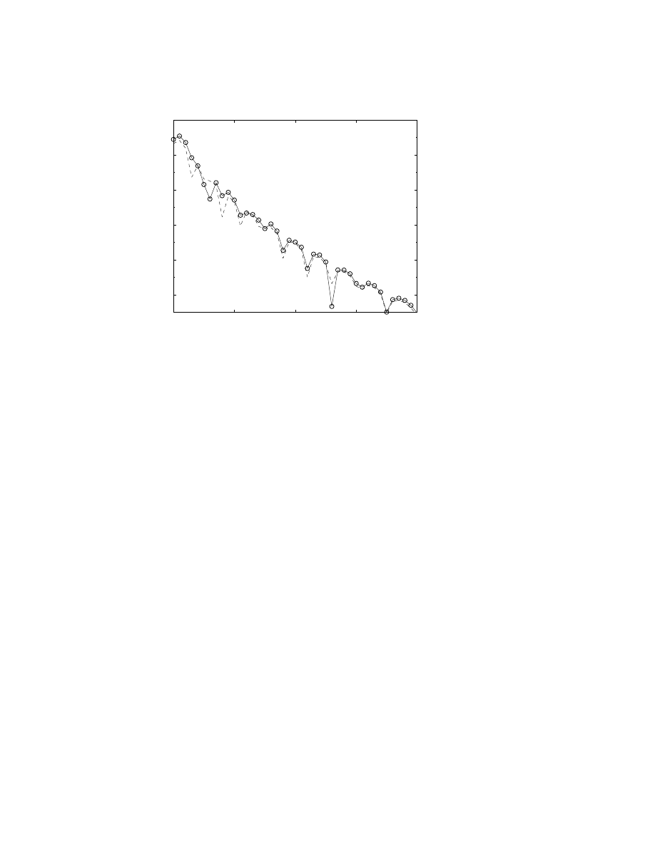
Exponential Asymptotics
71
0
10
20
30
40
10
-10
10
-8
10
-6
10
-4
10
-2
10
0
n
Figure 16. Solid with circles: The absolute values of the Chebyshev coefficients a
n
for the expansion of Berry’s superfactorial function, BeS(²; A = 4) on ²
∈ [0, 1].
The thin dashed curve, closely tracking the solid curve, illustrates the coefficients of
exp(
−2/²), which are known to decay as exp(−3 2
1/3
n
2/3
).
hyperasymptotics of the confluent hypergeometric function for every
one on the asymptotics of spectral series.
When exponentially small effects are present, there are often algo-
rithmic challenges present, too. Numerical checking of the prefactors
in front of exp(
−q/²) as obtained by the PKKS matched asymptotics
(or whatever) may be impossible in single precision because the expo-
nentially small quantity may fall below the single precision threshold
for moderate ², making it impossible to determine whether numerical
differences are due to errors in the asymptotics, or the neglected effects
of higher order terms at not-so-small ². When α was smaller by a factor
of 10
−48
than the core of the solitary wave, Boyd [71] numerically com-
puted the radiation coefficient α to a relative precision of six decimal
places by using 70 decimal place arithmetic in Maple.
These calculations would seem to be very expensive since (i) spectral
methods generate full matrices instead of the sparse matrices produced
by finite differences and (ii) multiple precision arithmetic is excruci-
atingly slow in comparison to single precision operations, which are
executed directly in silicon. However, most spectral solutions to bound-
ary value and eigenvalue problems are performed with preconditioning.
That is to say, the bulk of the code for solving a differential equation in
multiple precision with spectral accuracy is to write a low order finite
ActaApplFINAL_OP92.tex; 21/08/2000; 16:16; no v.; p.71

72
John P. Boyd
difference or finite element code to solve the inhomogeneous version of
the problem in single precision. By repeatedly calling this finite dif-
ference solver, evaluating the residual in multiple precision with spec-
tral methods at the end of each iteration, one can obtain a multiple
precision, spectrally accurate solution without ever factoring (or even
computing) the full, dense spectral matrix. By use of the Fast Fourier
Transform, the spectral evaluation of the residual of an ordinary differ-
ential equation can be performed at a cost that grows as O(N log
2
N )
operations where N is the number of degrees of freedom.
Another special difficulty that arises mostly in exponentially small
phenomena is that of solutions on the infinite interval which do not
decay to zero for
| x |,but rather to sinusoidal oscillations. Two good
strategies have been developed.
The first is to approximate the infinite interval by a large but spa-
tially periodic interval, and then expand the solution as a Fourier series.
The drawback is that the radiation coefficient α is sensitive to the spa-
tial period P (modulo the wavelength of the far field oscillations, W ).
However, the periodic solutions themselves are often interesting. (In
the atmosphere, for example, the solutions are always periodic in lat-
itude and longitude.) In addition, the parameter P/W is actually a
manifestation of a genuine degree of freedom, the “phase factor” Φ,
of the infinite interval. Consequently, it is possible to trace the entire
parameter space for the unbounded domain by using the device of a
large but periodic computational interval.
The second strategy is add one or more additional basis functions
which are chosen to mimic the required asymptotic behavior of the
“wings” of the weakly nonlocal solitary wave (or whatever). When
the width of the core structure is inversely proportional to ² and the
wavenumber of the wing oscillations is k
f
, an effective radiation basis
function is
φ
rad
(x)
≡ H(x+Φ; ²) sin(k
f
x+Φ)+H(
−x+Φ; ²) sin(k
f
−x+Φ) (132)
where a smoothed approximation to the step function is defined by
H(x; ²)
≡ (1/2){1 + tanh(²x)}
(133)
Boyd [60] has successfully applied a mixed basis of the rational Cheby-
shev polynomials[53] plus a single “radiation function” to compute
quantum scattering in one dimension. Boyd [62] shows that one can
construct a basis function that depends nonlinearly on its coefficient
— which is an approximation to α — so as to apply this method even
when the oscillations for large
| x | are allowed to weakly self-interact,
as is inevitable for nonlinear differential equations.
ActaApplFINAL_OP92.tex; 21/08/2000; 16:16; no v.; p.72

Exponential Asymptotics
73
Boyd[54] used rational Chebyshev functions on the semi-infinite
interval to approximate the J
0
Bessel function. This asymptotes to a
sinusoidal oscillation rather than decaying, so a naive expansion in basis
functions appropriate to an unbounded interval will fail disastrously.
Nevertheless, he wrote, in a form mimicking the large x asymptotics,
J
0
(x)
≈
1
p
(1 + x)
{P (x) cos(x − π/4) + Q(x) sin(x − π/4)}
(134)
Using a total of only 17 coefficients for P (x) and Q(x) combined gave a
maximum absolute error of less than 2
× 10
−7
uniformly on x
∈ [0, ∞].
Numerical methods to replace divergent power series do demand
some technology which is not otherwise widely used. It is encouraging
that now this technology mostly exists and has been tested in applica-
tions.
18. Numerical Methods, II: Sequence Acceleration and
Pad´
e and Hermite-Pad´
e Approximants
Sequence acceleration or “summability” methods have a long histo-
ry [139, 318, 315, 316]. The Euler sum acceleration is an elderly but
still potent algorithm as already shown for the Stieltjes function. It is,
however, but one of many schemes in the literature. We must refer to
specialized reviews [139, 318, 315, 316] for an in depth discussion, but
it is important to note one principle and one algorithm.
The principle is that acceleration methods are slaves to the oscilla-
tions of the j-th term in the series with respect to j. For alternating
series, that is, those for which the sign of the (j + 1)-st term is opposite
the sign of the j-th term, and for nearly alternating series, acceleration
methods are very effective. For monotonic series, that is, expansions
whose terms are all of the same sign, some different but effective accel-
eration schemes are also known [315, 316]. However, when the series
is slowly oscillating in degree j but not strictly monotonic, sequence
acceleration algorithms tend to perform very badly [70].
The [p/q] Pad´e approximant to a function f (²) is a polynomial of
degree p divided by a polynomial of degree q which is chosen so that
the leading terms of the power series of the approximant match the first
(p + q + 1) terms of the power series of f (²). The good news is that the
Pad´e approximation usually converges even when the power series from
whence it came diverges. For example, it has been rigorously proved
that the [N/N ] approximant to the Stieltjes function S(²) converges
with an error that decreases proportional to exp(
−4N
1/2
/²
1/2
) — in
ActaApplFINAL_OP92.tex; 21/08/2000; 16:16; no v.; p.73
74
John P. Boyd
other words, exponential but subgeometric convergence, similar to the
Chebyshev series for this function[19].
Unfortunately, the Pad´
e approximant fails along the branch cut for
the Stieltjes function, which is the negative real ²
− axis. Because the
integral that defines the Stieltjes function has a pole on the integration
path when ² is real and negative, the function is not completely specified
until we choose how the pole is treated. The Stieltjes function is real-
valued if the integral is interpreted as a Principal Value integral, but
has an imaginary part which is exponentially small in 1/² if the path
of integration is indented above or below the pole in the t-plane. That
is,
S(
−²) = P V
Z
∞
0
exp(
−t)
1
1
− ²t
dt
± i π
1
²
exp(
−1/²)
(135)
where the sign of the imaginary part depends on whether the contour
is idented above or below the real t
− axis. Since the terms in the
Stieltjes power series, S(²)
∼
P
∞
j=0
(
−1)
j
j!, are all real-valued, one can
prove that the coefficients of the numerator and denominator polyno-
mials in the Pad´e approximant are real, too. Even if the approximants
converged, they would inevitably miss the imaginary part of S(
−|²|).
The same difficulty arises in quantum mechanics. For the quartic
oscillator, for example, the eigenvalue E of the stationary Schr¨
odinger
equation is complex-valued when the coupling constant ² is negative;
physically, the imaginary part is the inverse of the lifetime of a metastable
bound state, which eventually radiates away from the local minimum
of the potential energy. The exact
=(E) is not analytically known, but
it does decrease exponentially fast with 1/
|²|. Because =(E) gives the
lifetime of the state, and therefore the rate of radiation, it is a very
important quantity even when small. Ordinary Pad´
e approximants fail
when ² is real and negative, however, just as for the Stieltjes function.
(In fact, it has been proved that both the eigenvalue of the quartic oscil-
lator and S(²) belong to a class of functions called Stieltjes fuctions,
and thus are close cousins.)
Shafer[282] developed a generalized Pad´
e approximant which has
been used successfully by several groups to calculate exponentially
small imaginary parts of quantum eigenvalues[300, 131, 280, 287, 281].
The approximant f [K/L/M ] is defined to be the solution of the quadrat-
ic equation
P (f [K/L/M ])
2
+ Q f [K/L/M ] + R = 0
(136)
where the polynomials P , Q and R are of degrees K, L and M , respec-
tively. These polynomials are chosen so that the power series expansion
ActaApplFINAL_OP92.tex; 21/08/2000; 16:16; no v.; p.74

Exponential Asymptotics
75
of f [K/L/M ] agrees with that of f through the first N = K +L+M +1
terms. (The constants in P and Q can be set equal to one without loss
of generality since these choices do not alter the root of the equation, so
the total number of degrees of freedom is as indicated.) As for ordinary
Pad´e approximants, the coefficients of the polynomials can be comput-
ed by solving a matrix equation and the most accurate approximations
are obtained by choosing the polynomials to be of equal degree, so-
called “diagonal” approximants.
Fig. 17 shows the diagonal approximant of the Stieltjes function for
negative real ²; the polynomials for the [4/4/4] approximation are
P = 1
− (160/3)² + (3680/3)²
2
+ (3680/3)²
3
+ 7240²
4
Q = 1 + (2239/9)²
− (2698/9)²
2
+ (43658/3)²
3
+ 5056²
4
R =
−2 − (1732/9)² − (7126/9)²
2
− (41504/3)²
3
− (2452/9)²
4
;
(137)
The two roots of the quadratic equation give us the result of choosing
to indent the contour either above or below the path of integration;
discarding the imaginary part gives the Principal Value of the integral.
The [10/10/10 approximant gives a maximum relative error for both
parts of less than 5
× 10
−6
.
Shafer’s idea can be generalized to polynomials of higher degree
in the approximation. The result is usually called a “Hermite-Pad´
e”
approximant. The quadratic or “Shafer” approximants seem to be quite
successful for most quantum problems[300, 131, 280, 287]. However,
Sergeev and Goodson describe fast algorithms for computing approxi-
mants of higher degree and also solve some problems where such high-
er degree approximants, capable of representing cube roots and higher
branch points, are very useful[281].
Pad´e approximants have been generalized in several other direc-
tions, too.[129]. Reinhardt [269] has developed a procedure using double
Pad´e approximants which works well even for monotonic, factorially-
diverging series, including the computation of exponentially small
=(E),
although it has been largely displaced by Shafer approximants. Anoth-
er generalization is to approximate f by the solution of an ordinary
differential equation([10] and earlier references cited there) or a partial
differential equation ([97] and earlier articles therein) where again the
coefficients of the differential equation are polynomials in ² chosen so
the approximant has a power series matching f up to some finite order.
Pad´e methods have limitations; they seem to be quite useless for
calculating the exponentially small radiation coefficient of a weakly
nonlocal solitary wave, for example. Nonetheless, many problems in
quantum mechanics have fallen to Hermite-Pad´e approximants.
ActaApplFINAL_OP92.tex; 21/08/2000; 16:16; no v.; p.75
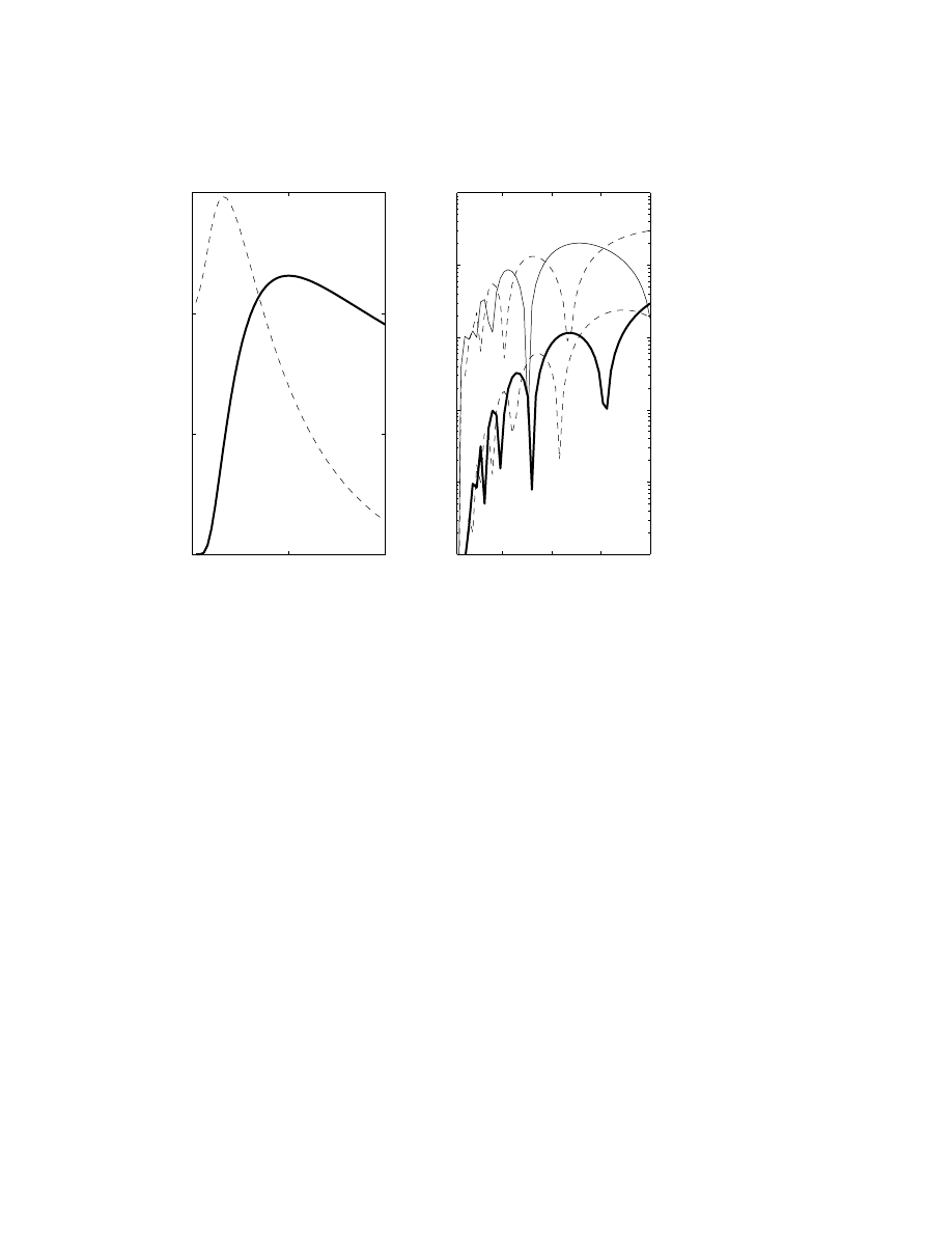
76
John P. Boyd
0
1
2
0
0.5
1
1.5
-
ε
ℑ
(S)
ℜ
(S)
Stieltjes func. S on the cut
0.5
1
1.5
2
10
-6
10
-5
10
-4
10
-3
10
-2
10
-1
-
ε
Abs. Errors: Shafer Approx.
[4/4/4]
[8/8/8]
Figure 17. Left panel: the real and imaginary parts of the Stieltjes function on
the negative real ²
− axis. Right: the absolute value of the absolute error for the
real part (thin dashed) and imaginary part (thick solid) part in the [4/4/4] Shafer
approximant (top pair of curves) and the [8/8/8] approximant (bottom solid and
dashed curves).
19. High Order Hyperasymptotics versus Chebyshev and
Hermite-Pad´
e Approximations
“I wrote an analytical solution to a sixth order differential equation
as a hypergeometric integral, derived asymptotic approximations,
matched the boundary conditions, and finally went to a computer
to make graphs. The machine took about a minute. Then I solved
the whole problem numerically, and the same machine took about
two seconds. That was the last analytical work I ever did!”
— R. E. Dickinson [115]
As illustrated by Dickinson’s amusing experience, very complicated
analytical answers are really just another form of numerical solution.
High order asymptotic and hyperasymptotic solutions are usually in
this category because a long string of terms adds little insight to the
ActaApplFINAL_OP92.tex; 21/08/2000; 16:16; no v.; p.76

Exponential Asymptotics
77
lowest term, only greater numerical accuracy. Consequently, a proverb
in perturbation theory is: One term: insight; several terms: numerics.
If many terms, as opposed to three or four terms, are available, it is
possible to deduce some non-numerical information from the series such
as the approximate location of the convergence-limiting singularities in
the complex plane (another use of Darboux’s Principle!) However, this
analytic information is mostly used only to transform the series to
improve the rate of convergence as described in van Dyke’s book[298],
for example. Fluid dynamicists are not too interested in branch points
at complex values of the spatial coordinates!
In the rest of this section, we shall focus on answering the question
suggested by these considerations: How useful are high order hyper-
asymptotics numerically in comparison to other numerical methods?
Although many books and articles on beyond-all-orders methods
offer numerical tables, head-to-head comparisons between hyperasymp-
totics and other numerical algorithms are rare. Most of the work cata-
logued in Table IV has a decidely pre-computer spirit.
One reason for this lack of efficiency contests is that most software
libraries already have quite efficient routines for computing special func-
tions. Typically, the algorithms for computing Bessel and Airy func-
tions, the Error Integral, and so on employ two expansions for each
function. Through experimentation and theory, a breakpoint ζ is cho-
sen for each function. A convergent power series is used for
| z |≤ ζ
whereas a divergent expansion in form of an exponential or trigonomet-
ric pre-factor multiplied by a series of inverse powers of z is employed
for
| z |> ζ. (The divergent series may actually be different expansions
in different parts of the complex plane because of Stokes’ phenomenon.)
Hyperasymptotics might seem like a natural way to add a few decimal
places of additional accuracy.
Unfortunately, the extension beyond the superasymptotic approxi-
mation is a series of terminants like Eq.(73). Olde Daalhuis[240, 242]
has developed good numerical methods for evaluating terminants, but
the approximations are series of hypergeometric functions which can
only be evaluated by recurrence. This implies that each terminant is
itself as expensive to evaluate as the special function it helps to approx-
imate. Thus, terminant series are numerically inefficient. It is probably
more sensible to simply increase the “break point” where the subrou-
tine switches from the power series to the inverse power series and also
increase the number of terms in each series.
In practice, both series are replaced by the equivalent Chebyshev
series, which converge faster and also are much more resistant to round-
off error. It is useful to illustrate how easily these expansions can be
derived to replace the standard divergent asymptotic series.
ActaApplFINAL_OP92.tex; 21/08/2000; 16:16; no v.; p.77

78
John P. Boyd
For example, the Stieltjes function S(²) satisfies the ordinary differ-
ential equation
²
2
d S
d²
+ (1 + ²)S = 1
(138)
For paper-and-pencil or symbolic language calculation, the simplest
method is the “Lanczos τ -method”. He observed [177, 284] that if we
perturb the right-hand side of Eq.(138) by a polynomial of degree M ,
multiplied by an unknown constant τ , we can then solve this perturbed
equation exactly by a polynomial of degree M . (Instead of the usual
strategy of approximately solving the exact differential equation, the
τ -method exactly solves an approximate differential equation.) If the
perturbing polynomial is ²
M
, then the τ -method yields the first M
terms of the usual divergent power series in ².
However, this is actually a rather stupid choice if the goal is uniform
accuracy on some interval ²
∈ [0, z] where z is a complex number. The
power function ²
M
is extremely non-uniform — very small near the
origin, but increasing very rapidly away from it. The polynomial of
degree M (and leading coefficient of one) which is most uniform on
[0, z] is the shifted Chebyshev polynomial T
∗
M
(²/z) [177, 178, 55].
Table VI is a short code in the symbolic manipulation language
Maple to solve the ordinary differential equation
²
2
d S
d²
+ (1 + ²)S = 1 + τ T
∗
M
(²/z)
(139)
through a Chebyshev τ
− method. The most important feature of the
table is simply its brevity: all the necessary algebra is performed in
exact, rational arithmetic under the control of only nine lines of code!
The choice of Maple is arbitrary; the same calculation could be per-
formed with equal brevity in any of the other widely used symbolic alge-
bra languages including Mathematica, MACSYMA and Reduce. Boyd
[55, 63] gives many examples of problem-solving via spectral methods
in algebraic manipulation languages. Note that because all operations
involve polynomials, not transcendentals, the code also executes very
speedily.
The Chebyshev-τ result is rather messy: polynomial in ², rational
in z. However, the Chebyshev (or Chebyshev-like) expansion will obvi-
ously converge most rapidly when the expansion interval [0, z] is small
as possible for a given ². This implies that for best results, one should
choose z = ². Making this substitution not only optimizes accuracy for
a given ², but also simplifies the result to a rational function of ² alone.
The M = 8 approximation, which is a polynomial of degree 7 over a
polynomial of degree 8, is
S
8
≡ 16 {4 + 124² + 1336²
2
+ 6168²
3
+ 12173²
4
+ 8955²
5
+ 1737²
6
+ 33²
7
}/
ActaApplFINAL_OP92.tex; 21/08/2000; 16:16; no v.; p.78

Exponential Asymptotics
79
{256 + 8192² + 93184²
2
+ 473088²
3
+ 1108800²
4
+1128960²
5
+ 423360²
6
+ 40320²
7
+ 315²
8
}
(140)
Fig. 18 shows that for small positive ², this simple rational approxima-
tion is on the whole a lot more useful than either the superasymptotic
or hyperasymptotic series.
Chebyshev polynomial approximations are usually polynomials rather
than rational functions and are optimized for a particular line segment
in the complex plane. By computing symbolically, we have obtained an
approximation that is more complicated (because it is rational rather
than polynomial) but has the great virtue of being as accurate, for a
given ², as the standard Chebyshev approximation of degree M along
the segment [0, ²] even when ² is complex-valued.
In the previous section, we have already given the ordinary asymp-
totics of the Chebyshev coefficients of the Stieltjes function. However,
the comparison of convergent Chebyshev series with divergent power
series is not completely straightforward. The asymptotic series uses a
number of terms N which is inversely proportional to ². What happens
if we compare the N -term Chebyshev series on the interval ²
∈ [0, 1/N]
with the N -term optimally truncated power series for ² = 1/N ?
Through an elementary steepest descent analysis of the usual inner
product integrals for the coefficients of an orthogonal series,, one finds
that the N -th Chebyshev coefficient for the series on [0, 1/N ] is (pre-
viously unpublished)
a
N
∼ 2.98
√
N exp(
−2.723N)
∼ 2.98²
−1/2
exp(
−2.723/²)
(141)
(One can show that the error in truncating the Chebyshev series after
N terms is proportional to a
N
[55, 73].) Intriguingly, the errors for Pad´
e
approximants and for hyperasymptotics are of this same form:
|f − f
N
| ≤ exp(−q/²),
N
∼ O(1/²)
(142)
where the constant q > 0 depends on the precise Chebyshev, Pad´e,
or hyperasymptotic scheme used. There are likely deep connections
between these different families of approximations which are now only
dimly understood [51].
One can make more entertaining approximations by using other
spectral basis sets. For example, the rational Chebyshev functions are a
good basis set for the semi-infinite interval, x
∈ [0, ∞]. Boyd [54] gives
three examples in which the usual pair of series – divergent series in 1/x
for large x and convergent power series for small x – can be replaced
by a single expansion over the entire semi-infinite range. The examples
ActaApplFINAL_OP92.tex; 21/08/2000; 16:16; no v.; p.79

80
John P. Boyd
range from the K
1
Bessel function, which has a pole at the origin, to
the J
0
Bessel function, in which separate series multiply the sine and
cosine in the uniform approximations, to the ground state eigenvalue
of the quantum quartic oscillator as a function of the coupling constant
², which is a Stieltjes function with a factorially divergent power series
about ² = 0 [47, 19]. These uniform approximations are much compli-
cated and converge more slowly than the pair of Chebyshev series they
replace, but have the advantage of avoiding a conditional statement,
which is needed in the traditional approach to switch between large
and small x approximations.
Lastly, one must not overlook non-series alternatives. Schulten, Ander-
son and Gordon [277] have developed an efficient subroutine to evaluate
the Airy functions at arbitrary points in the complex plane. Instead of
using an asymptotic approximation for large
| z |, they use a clever
optimized Gaussian quadrature to directly evaluate the integral repre-
sentations for Ai and Bi, even on Stokes’ lines. Their double precision
code, which is accurate to at least 11 decimal places for all
| z | (with
use of the power series about z = 0 near the origin) employs a maximum
of just six quadrature points!
Detailed comparisons between high order hyperasymptotics and oth-
er methods of numerical approximation have not yet been carried out.
Still, the examples and illustrations above show that the comparison,
except perhaps for special cases, is likely to be unfavorable to high
order asymptotics.
Although hyperasymptotics look comparable to Chebyshev and Pad´
e
schemes when N
∼ O(²), the Chebyshev and Pad´e have the profound
advantage of converging as N
→ ∞ for fixed ². Furthermore, these
approximations are built from ordinary polynomials whereas hyper-
asymptotic approximations are series of hyperterminants, which in turn
are approximated by series of hypergeometric functions.
There may be a few exceptions: problems where no alternatives
are available. In quantum chaology, Gutzwiller’s divergent series for
the quantum spectrum has been summed using resurgence[182, 39].
The practical result has been greatly improved energies for quantum
mechanics odd-shaped billiard tables – idealized but popular for test-
ing theories [182, 39]. Another application is computing the zeros of the
Riemann zeta function, where resurgence has proved to be much better
than the best available competitor, the (un-resurgent) Riemann-Siegel
formula [34].
Berry’s amusing quote,“I am not expecting an early call”, is a frank
admission that most extensions of exponential asymptotics beyond the
lowest nontrivial term are arithmurgically useless. The proper use of
exponential asymptotics is to give insight. A sensible application is to
ActaApplFINAL_OP92.tex; 21/08/2000; 16:16; no v.; p.80
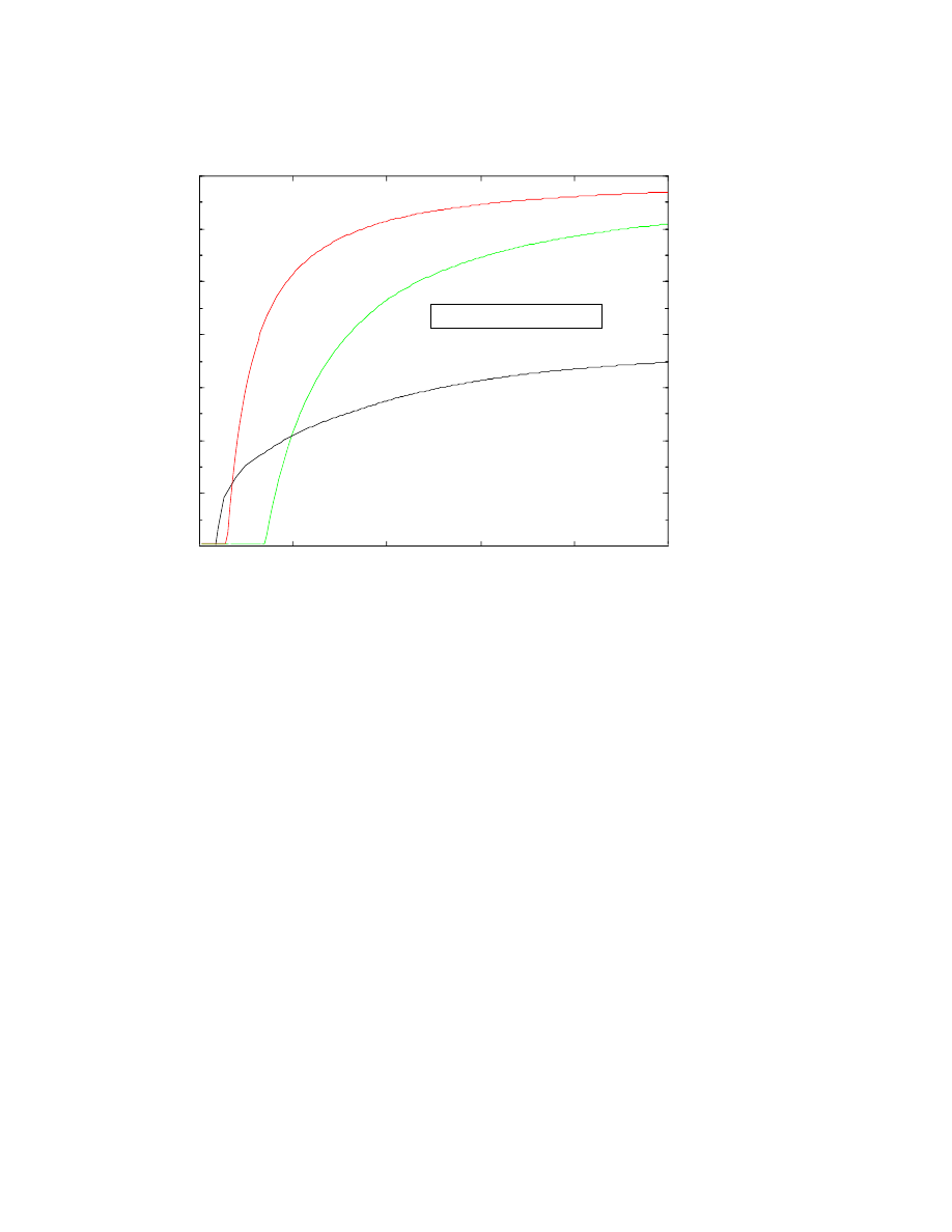
Exponential Asymptotics
81
AAAAAAAAAAAAAAA
AAAAAAAAAAAAAAA
AAAAAAAAAAAAAAA
AAAAAAAAAAAAAAA
AAAAAAAAAAAAAAA
AAAAAAAAAAAAAAA
AAAAAAAAAAAAAAA
AAAAAAAAAAAAAAA
AAAAAAAAAAAAAAAAA
AAAAAAAAAAAAAAAAA
AAAAAAAAAAAAAAAAA
AAAAAAAAAAAAAAAAA
AAAAAAAAAAAAAAAAA
AAAAAAAAAAAAAAAAA
AAAAAAAAAAAAAAAAA
AAAAAAAAAAAAAAAAA
AAAAAAAAAAAAAAAAA
AAAAAAAAAAAAAAAAA
AAAAAAAAAAAAAAAAA
AAAAAAAAAAAAAAAAA
H
yp
er
as
ym
pto
tic
s&
Che
bysh
ev
0
0.1
0.2
0.3
0.4
0.5
10
-14
10
-12
10
-10
10
-8
10
-6
10
-4
10
-2
10
0
ε
AAA
AAA
AAA
AAA
Higher Order
Chebyshev Only
All Methods
Chebyshev Only
Figure 18. A comparison of the rational τ -Chebyshev approximation S
8
versus the
superasymptotic and hyperasympotic approximations for the Stieltjes function, S(²).
The three solid curves plot the errors for each of the three methods versus ². If
acceptable accuracy for a given ² is a point in the unshaded region in the upper
left corner, all three methods are satisfactory. In the unshaded lower right region,
none of the three approximations is sufficiently good (although such tiny errors
< 1
× 10E
−12
can be achieved by simply using a Chebyshev τ approximation of
higher order). The vertical shading – most of the graph – shows where the Chebysehv
approximation S
8
, a polynomial of degree 7 divided by degree 8, is successful, but
the asymptotic series fail because their minimum error is larger than the required
tolerance. In the vertically-and-horizontally shaded area, both hyperasympotics and
S
8
(²) are successful. Finally, there is a tiny region of horizontal shading where only
hyperasymptotics is successful (though a Chebyshev approximation of higher order
than S
8
(²) would succeed). The hyperasymptotic errors were calculated using the
Berry-Howls scheme (where the errors are O(exp(
−2.386/²)), but employing the
more accurate hyperasymptotic methods of later authors such as Olde Daalhuis
would not change the theme of the graph.
compute a small term that is also the leading term to approximate
some crucial feature of a problem, perhaps the lifetime of a quantum
bound state or a nonlocal solitary wave.
ActaApplFINAL_OP92.tex; 21/08/2000; 16:16; no v.; p.81

82
John P. Boyd
20. Hybridizing Asymptotics with Numerics
The hyperasymptotic scheme of Boyd [68] and the PKKS method
[171, 172] are both blends of analysis and numerics in the sense that
the final step, the determination of the proportionality constant which
multiplies the exponential of 1/², requires a computation. However, the
prior analysis has reduced the problem to a very small calculation that
returns an answer as the product of a number with an analytical fac-
tor. This is far different than a brute force calculation that requires a
hundred times as much computer time to return only a number.
The flow past a sphere or cylinder at small Reynolds number Re[264,
159, 161, 160, 98, 283]. has frustrated fluid dynamicists for over forty
years, but there has been, very recently, a partial breakthrough by
means of a hybrid numerical-asymptotic method [170]. The source
of pain is that these expansions are double series in powers of Re
and 1/ log(Re) or, defining ² = 1/ log(Re), in powers of exp(
−1/²)
and ². Formally, one should include an infinite number of logarithmic
corrections to the drag coefficient before computing the first correc-
tion proportional to Re. For the flow past the circle, however, Re >
(1/ log(3.70/Re))
4
for all Re > 1/12000. (Real fluid flows are typical-
ly at much larger Re.). A systematic scheme for the transcendentally
small terms is still an open problem. For the sphere, which is probably
the easier of the two, Chester and Breach conclude sadly “the expan-
sion is of practical value only in the limited range Re < 1/2 and that
in this range there is little point in continuing the expansion further”.
Kropinski, Ward and Keller [170] made the crucial observation that
if the outer (“Oseen”) problem is solved numerically, the numerical
solution will implicitly incorporate an infinite number of logarithmic
corrections. Better yet, the outer solution is independent of whether the
body is a cylinder, an elliptic cylinder, or some other smooth shape: a
single numerical solution provides a good answer to a whole spectrum
of body shapes. The inner solution differs from shape to shape, but
is easy to calculate analytically. They have successfully applied this
same idea, outer-numerical/inner-analytical, to other problems with
logarithmic corrections [308]. The end product neglects higher powers
of ² and the necessary numerics is the full solution to a PDE, but still,
their work is real progress after two decades of no advance at all.
It seems likely that such hybrid numerical-asympotic methods will
flourish in the next few years for following reasons:
− Analytical perturbation theory has enjoyed at least a century of
development, and it is hard to grow good ideas in such old soil.
ActaApplFINAL_OP92.tex; 21/08/2000; 16:16; no v.; p.82

Exponential Asymptotics
83
− Mathematics departments, even in the non-computational areas,
are becoming more computer-friendly.
− Hyrid algorithms have successfully attacked a number of problems
already.
− There are broad areas where hybrids have not yet been tried.
21. History
Improving upon the minimum error of an asymptotic series has a long
history; Stieltjes himself discussed the possibility in his 1888 doctoral
thesis. Oppenheimer’s calculation of the exponentially large decay time
in the quantum Stark effect and the independent discovery of quantum
tunnelling by Gamow and by Condon and Gurney all happened in 1928.
The Euler acceleration of the Stieltjes function series was first analyzed
by Rosser [273] in 1951.
One can distinguish several parallel lines of development. The first is
the calculation of “converging factors” or terminants for the asymptotic
expansions of special functions, beginning with Airey in 1937 [3] and
reaching a high degree of sophistication in the books of Dingle (1973)
and Olver(1974) [118, 249], who also give good histories of earlier work.
Another was quantum mechanics, beginning with discovery of tun-
nelling in 1928, continuing with the Pokrovskii-Khalatnikov solution for
“above-the-barrier” quantum scattering, and continued to the present
with studies of high order perturbation theory. The books written by
Arteca, Fernandez and Castro [8] and edited by LeGuillou and Zinn-
Justin[181] and Braaksma[83] are good testaments, as is a special issue
of International Journal of Quantum Chemistry[269].
A third area is KAM theory and dynamical systems theory in gener-
al. Under perturbations, integrable dynamical systems become chaot-
ic, but the chaos is confined to exponentially thin regions around the
separatrices [136] for small ². Through “Arnold diffusion”, dynamical
systems can move great distances in phase space (on exponentially long
time scales) even when the perturbation is very weak.
A fourth area is “weakly nonlocal solitary waves”, that is, nonlin-
ear coherent structures that would be immortal were it not for weak
radiation away from the core of the structure. These seem to be as
ubiquitous as classical, decaying-to-zero solitary waves. Nonlocal soli-
tary waves arise in fiber optics, hydrodynamics, plasmas and a wide
variety of other applications. Meiss and Horton (1983) [201] seem to
have done the earliest explicit calculations. However, the existence of
ActaApplFINAL_OP92.tex; 21/08/2000; 16:16; no v.; p.83

84
John P. Boyd
slowly radiating solitary waves in particle physics (“ φ
4
breathers”) and
oceanography (Gulf Stream Rings) was known from observations and
initial value computations a decade earlier. The subsequent eruption of
activity is catalogued in the book by Boyd [72].
A fifth area is crystal formation and solidification. The 1985 work
of Kruskal and Segur [171, 172] resolved a long-standing roadblock in
the theory of dendritic fingers on melt interfaces, and touched off a
great plume of activity. There was rapid cross-fertilization with nonlo-
cal solitary waves because Segur and Kruskal applied their new PKKS
method to the “φ
4
breather” of particle physics, contributing to the
rapid growth of exponential asymptotics for nonlinear waves.
A sixth area is fluid mechanics. The Berman-Terrill-Robinson prob-
lem [135] in flows with suction, the radiative decay of free oscillations
bound to islands [185] and Kelvin wave instability in oceanography
and atmospheric dynamics [74, 75] were all examples in which expo-
nential smallness had been calculated in the seventies or early eighties.
Somehow, these problems remained isolated. However, boundary layer
theory always involves divergent power series and exponential smallness
as showed by example above. Fluids is an area where hyperasymptotic
technology is likely to have a vigorous future.
A seventh line of research is that pursued by Richard E. Mey-
er and his students. This began with studies of adiabatic invariants
[202, 203, 204, 219, 205, 207]. He also devised an independent solu-
tion to “above the barrier” quantum scattering: recasting the problem
as an integral equation so that the reflection coefficient appears as
the dominant contribution instead of as an exponentially small cor-
rection [206, 208]. This led to further studies of exponential smallness
in water waves trapped around an island [185, 209, 220], connection
across WKB turning points and wave dynamics and quantum tun-
nelling [221, 211, 222, 223, 224, 212, 214, 215, 216, 225, 218, 226].
Meyer has also written four reviews [210, 213, 217, 218].
An eighth line of development is the abstract theory of resurgence
and multisummability. This began with ´
Ecalle[123] and continued with
important contributions from Pham, Ramis, Delabaere, Braaksma and
others too numerous to mention as reviewed in [285, 83, 15].
Lastly, a ninth area is the development of resurgence and Stokes
phenomenon by physicists and applied mathematicians. This grew out
of the abstract theory of ´
Ecalle, which Berry learned during a visit to
France, but took resurgence in a direction that was less rigorous but
much more pragmatic and applied. The trigger was Berry’s 1989 real-
ization that the discontinuity in the numerical value of an asymptotic
expansion at a Stokes’ line could be smoothed. (The change in topology
of the steepest descent path at a Stokes lines is unavoidable, howev-
ActaApplFINAL_OP92.tex; 21/08/2000; 16:16; no v.; p.84

Exponential Asymptotics
85
er.) Building on the books of Dingle, Olver and ´
Ecalle, Berry, Howls,
Olver, Olde Daalhuis, Paris, Wood, W. G. C. Boyd and others have
developed smoothed, high order hyperasymptotic approximations for
many species of special functions, for the WKB method and for other
schemes for differential equations. A selection is given in Table IV.
Dingle’s ideas of generic forms for the late terms in asymptotic series
and universal terminants now seem as important to the rise of exponen-
tial asymptotics as the comet-crash(?) that put an end to the dinosaurs
was in biology. Only a year later, Olver’s book developed similar ideas,
with error bounds, for ordinary differential equations. And yet, though
these books were widely bought and read, their net effect at the time
was as quiet as a sandcastle washed away by a rising tide. Bothered by
long-term illness, Dingle never published again.
In recent years, however, the analysis of exponentially small terms
has exploded. A special program of study at the Newton Institute at
Cambridge has brought together researchers from a wide range of fields
for a workshop lasting the whole first half of 1995. The books by Boyd
[72] and Segur, Tanveer and Levine (eds.) [279] are good introductions
to the vigour and diversity of this interest.
Why was this revolution in asymptotics so slow, so long delayed?
Perhaps the most important factor is that alterations in scientific world-
view, like atom bombs, require assembling a critical mass. Part of this
critical mass was provided by the parallel threads of slow develop-
ment outlined above; when ideas began to cross disciplinary boundaries,
exponential asymptotics exponentiated. Another trigger was the pop-
ularization of algebraic manipulation languages, which made it easier
to compute many terms of an asymptotic series. Lastly, applied math-
ematics is subject to fads and enthusiasms.
I myself read both the Dingle and Olver books when they first
appeared while I was still in graduate school, but was unimpressed.
First, my ² was not very small. Second, a string of messy hyperasymp-
totic corrections seemed a poor alternative to numerical algorithms,
which were fast and efficient even a quarter century ago. Modern expo-
nential asymptotics still shares these limitations, but there is now a
cadre of enthusiasts who are unbothered as there was not in Dingle’s
time.
6
Still, with the emergence of exponential asymptotics as a subfield
of its own with ideas shared widely from physics to fluids to nonlin-
ear optics, hyperasymptotics has been very useful, at least as the low-
est hyperasymptotic order, in a wide variety of practical applications.
6
In a language of Papua New Guinea, the word “mokita” is used to denote
“things we all know but agree not to talk about”.
ActaApplFINAL_OP92.tex; 21/08/2000; 16:16; no v.; p.85

86
John P. Boyd
When the parallel threads ceased to be parallel and converged, the
ancient topic of asymptotics suddenly became very interesting again.
22. Books and Review Articles
The theme of extending asymptotic series through Borel summation
and other methods of re-expanding remainder integrals is treated in the
classic books of Dingle[118] and Olver[249]. Jones’ 1997 book is very
short (160 pages), a primer of steepest descent and hyperasymptotics
that is perhaps closest in style and spirit to the Dingle and Olver books,
but at a somewhat more elementary level. It includes a short appendix
on non-standard analysis as well as exercises at the end of each chapter.
´
Ecalle’s 1981 three-volume treatise greatly extended and generalized
earlier ideas on hyperasymptotics. Unfortunately, his work has not been
translated from French. However, Sternin and Shatalov is a recent pre-
sentation of the abstract theory of resurgence[285]. The collection of
articles edited by Braaksma[83] gives a broader but less coherent state
of the abstract resurgence work. Balser[15] is only one hundred pages
long, but is very readable, based on a course taught by the author.
Kowalenko et al.[169] is a short monograph devoted entirely to the
hyperasymptotics of a fairly narrow class of integrals. Maslov[199] is a
broad treatment of the WKB method.
Segur, Tanveer and Levine[279] is a collection of articles from a
NATO Workshop that displays the remarkable breadth of application
of beyond-all-orders asymptotics that existed even in 1991. Arteca, Fer-
nandez and Castro[8] and LeGuillou and Zinn-Justin [181] describe the
calculation of exponentially small terms in quantum mechanics through
large order perturbation theory and summation methods. Boyd[72] is
focused particularly on nonlocal solitary waves, but it includes a chap-
ter on general applications of hyperasymptotics and several chapters
on numerical methods.
Curiously, review articles seem rarer than books. Berry and Howls[39],
Paris and Wood[260] and Wood[320] have written short, semi-popular
reviews. Delabaere[112] has written (in English) an introduction to
´
Ecalle alient calculus. Olde Daalhuis and Olver[248] describe hyper-
asymptotics (and numerical methods) for linear differential equations.
Byatt-Smith[87],based on an unpublished but widely circulated manuscript
of seven years earlier, is not technically a review, but it nonetheless is
one of the most readable treatments of re-expansion of remainder inte-
grals and the error function smoothing of Stokes phenomenon.
ActaApplFINAL_OP92.tex; 21/08/2000; 16:16; no v.; p.86

Exponential Asymptotics
87
This profusion of books and reviews is helpful, but there are still
some large gaps. This present article was written to fill in some of
these holes and point the reader to other summaries of progress.
23. Summary
“What they [engineers] want from applied mathematics . . . is infor-
mation that illuminates.”
— Richard E. Meyer (1992) [218][pg. 43]
Key concepts:
− Divergence is a disease caused by a perturbative approximation
which is true for only part of the interval of integration or part of
the Fourier spectrum.
− A power series is asymptotic when the perturbative assumption is
bad only for a part of the spectrum or integrand that makes an
exponentially small contribution.
− When a factorially divergent series is truncated at its smallest
term, this “optimal truncation” gives an error which is typically
an exponential function of 1/². The usual Poincar´e definition of
asymptoticity, which refers only to powers of ², is therefore rather
misleading. The neologism “superasymptotic” was therefore coined
by Berry and Howls to describe the error in an optimally-truncated
asymptotic series.
− By appending one or more terms of a second asymptotic series
(with a different rationale) to the optimal truncation of a divergent
series, one can reduce the error below that of the superasymptot-
ic approximation to obtain a “hyperasymptotic” approximation.
This, too, is divergent, but with a minimum error far smaller than
the best “superasymptotic” approximation. (This rescale-and-add-
another-series step can be repeated for further error reduction.)
− There are many different species of hyperasymptotic methods includ-
ing:
1. sequence acceleration schemes such as the Euler, Pad´e and
Hermite-Pad´e (Shafer) approximations.
2. complex-plane matched asymptotics (the Pokrovskii-Khalatnikov-
Krusal-Segur method)
ActaApplFINAL_OP92.tex; 21/08/2000; 16:16; no v.; p.87

88
John P. Boyd
3. Resurgence schemes
4. isolation of exponential smallness
5. special numerical algorithms, usually employing Chebyshev or
Fourier spectral methods or Gaussian quadrature
− The history of exponential asymptotics stretches back at least a
century with several parallel lines of slow development that reached
a critical mass only within the last six years, culminating in an
explosion of both applications and theory that will touch almost
every field of science and engineering as well as mathematics
The list of open problems is large. One is a rigorous numerical test of
many-term, high order hyperasymptotic expansions versus competing
methods, such as Chebyshev series, for special function software. (The
arguments presented above suggest that the results are likely to be
unfavorable to hyperasymptotics).
Another is to create an expanded theory for the connection between
the rate of growth of power series coefficients or other properties of
functions with divergent power series and the rate of convergence of
Chebyshev series and Pad´e approximants. Some theorems exist for the
special class of Stieljtes functions (Chebyshev: [49, 51] and Pad´
e: [19]),
but little else.
An important issue is whether the Dingle terminant formalism can
be extended to weakly nonlocal solitary waves. The radiation coefficient
α, which is proportional to the function exp(
−µ/²) for some constant
µ, has only the trivial power series 0 + 0
· ² + 0 · ²
2
+ . . .. Does α
somehow influence the coefficients of the ² power series subtly so that
terminants can be applied, or is the radiation condition truly a ghost,
forever invisible to methods that look only at the asymptotic form of
the power series coefficients?
A fourth domain of future study is to apply exponential asymptotics
to new realms. We have shown above that the theory of numerical
algorithms contains hidden beyond-all-orders terms, but this aspect of
numerical analysis is largely terra incognita.
Although applications and fundamental research on exponential-
ly small terms will doubtless continue for many years, we have tried
to show that the underlying principles are neither complicated nor
obscure.
Acknowledgments
This work was supported by the National Science Foundation through
grant OCE9119459 and by the Department of Energy through contract
ActaApplFINAL_OP92.tex; 21/08/2000; 16:16; no v.; p.88

Exponential Asymptotics
89
KC070101. I thank Richard Meyer, Michael Ward and Robert O’Malley
for helpful correspondence or conversations, and others too numerous
to mention for supplying reprints and references. I am grateful to the
three referees for their extremely careful reading of this long paper.
References
1.
R.
C.
Ackerberg
and
R.
E.
O’Malley,
Jr.
, Boundary layer problems
exhibiting resonance, Stud. Appl. Math., 49 (1970), pp. 277–295.
Clas-
sical paper illustrating the failure of standard matched asymptotics; this
can be resolved by incorporating exponentially small terms in the analysis
(MacGillivray, 1997).
2.
T. C. Adamson, Jr. and G. K. Richey
, Unsteady transonic flows with shock
waves in two-dimensional channels, J. Fluid Mech., 60 (1973), pp. 363–382.
Show the key role of exponentially small terms.
3.
J. R. Airey
, The “converging factor” in asymptotic series and the calculation
of Bessel, Laguerre and other functions, Philosophical Magazine, 24 (1937),
pp. 521–552. Hyperasymptotic approximation to some special functions for
large
|x|.
4.
T. R. Akylas and R. H. J. Grimshaw
, Solitary internal waves with oscil-
latory tails, J. Fluid Mech., 242 (1992), pp. 279–298. Theory agrees with
observations of Farmer and Smith (1980).
5.
T. R. Akylas and T.-S. Yang
, On short-scale oscillatory tails of long-wave
disturbances, Stud. Appl. Math., 94 (1995), pp. 1–20. Nonlocal solitary waves;
perturbation theory in Fourier space.
6.
G. Alvarez
, Coupling-constant behavior of the resonances of the cubic anhar-
monic oscillator, Phys. Rev. A, 37 (1988), pp. 4079–4083. Beyond-all-orders
perturbation theory in quantum mechanics.
7.
V.
I.
Arnold
, Mathematical Methods of Classical Mechanics, Springer-
Verlag, New York, 1978. Quote about why series diverge: pg.395.
8.
G. A. Arteca, F. M. Fernandez, and E. A. Castro
, Large Order Per-
turbation Theory and Summation Methods in Quantum Mechanics, Springer-
Verlag, New York, 1990. 642pp.; beyond-all-orders perturbation theory.
9.
G. A. Baker, Jr. and P. Graves-Morris
, Pade Approximants, Cambridge
University Press, New York, 1996.
10.
G.
A.
Baker,
Jr.,
J.
Oitmaa,
and
M.
J.
Velgakis
, Series analysis of
multivalued functions, Phys. Rev. A, 38 (1988), pp. 5316–5331. Generaliza-
tion of Pad´
e approximants; the power series for a function u(z), known only
through its series, is used to define the polynomial coefficients of a differential
equation, whose solution is then used as an approximation to u.
11.
R. Balian, G. Parisi, and A. Voros
, Quartic oscillator, in Feynman Path
Integrals, S. Albeverio, P. Combe, R. Hoegh-Krohn, G. Rideau, M. Siruge-
Collin, M. Sirugue, and R. Stora, eds., no. 106 in Lecture Notes in Physics,
Springer–Verlag, New York, 1979, pp. 337–360.
12.
W.
Balser
, A different characterization of multisummable power series,
Analysis, 12 (1992), pp. 57–65.
13.
, Summation of formal power series through iterated Laplace integrals,
Math. Scand., 70 (1992), pp. 161–171.
14.
, Addendum to my paper: A different characterization of multisummable
power series, Analysis, 13 (1993), pp. 317–319.
15.
, From Divergent Power Series to Analytic Functions, vol. 1582 of Lec-
ture Notes in Mathematics, Springer-Verlag, New York, 1994. 100 pp.; good
presentation of Gevrey order and asymptotics and multisummability.
ActaApplFINAL_OP92.tex; 21/08/2000; 16:16; no v.; p.89

90
John P. Boyd
16.
W.
Balser,
B.
L.
J.
Braaksma,
J.-P.
Ramis,
and
Y.
Sibuya
, Multi-
summability of formal power series of linear ordinary differential equations,
Asymptotic Analysis, 5 (1991), pp. 27–45.
17.
W. Balser and A. Tovbis
, Multisummability of iterated integrals, Asymp-
totic Analysis, 7 (1992), pp. 121–127.
18.
L. Benassi, V. Grecchi, E. Harrell, and B. Simon
, Bender-Wu formula
and the Stark effect in hydrogen, Phys. Rev. Letters, 42 (1979), pp. 704–707.
Exponentially small corrections in quantum mechanics.
19.
C.
M.
Bender
and
S.
A.
Orszag
, Advanced Mathematical Methods for
Scientists and Engineers, McGraw-Hill, New York, 1978. 594 pp.
20.
C.
M.
Bender
and
T.
T.
Wu
, Anharmonic oscillator, Phys. Rev., 184
(1969), pp. 1231–1260.
21.
, Anharmonic oscillator. II. A study of perturbation theory in large order,
Phys. Rev. D, 7 (1973), pp. 1620–1636.
22.
E.
Benilov,
R.
H.
Grimshaw,
and
E.
Kuznetsova
, The generation of
radiating waves in a singularly perturbed Korteweg-deVries equation, Physica
D, 69 (1993), pp. 270–276.
23.
A. S. Berman
, Laminar flow in channel with porous walls, J. Appl. Phys., 24
(1953), pp. 1232–1235. Earliest paper on an ODE (Berman-Robinson-Terrill
problem) where exponentially small corrections are important.
24.
M.
V.
Berry
, Stokes’ phenomenon; smoothing a Victorian discontinuity,
Publicationes Mathematiques IHES, 68 (1989), pp. 211–221.
25.
, Uniform asymptotic smoothing of Stokes’s discontinuities, Proc. Roy.
Soc. London A, 422 (1989), pp. 7–21.
26.
, Waves near Stokes lines, Proc. Roy. Soc. London A, 427 (1990),
pp. 265–280.
27.
, Histories of adiabatic quantum transitions, Proc. Roy. Soc. London A,
429 (1990), pp. 61–72.
28.
, Infinitely many Stokes smoothings in the Gamma function, Proc. Roy.
Soc. London A, 434 (1991), pp. 465–472.
29.
, Stokes phenomenon for superfactorial asymptotic series, Proc. Roy.
Soc. London A, 435 (1991), pp. 437–444.
30.
, Asymptotics, superasymptotics, hyperasymptotics, in Asymptotics
Beyond All Orders, H. Segur, S. Tanveer, and H. Levine, eds., Plenum, Ams-
terdam, 1991, pp. 1–14.
31.
, Faster than Fourier, in Quantum Coherence and Reality: in Celebra-
tion of the 60th Birthday of Yakir Aharonov, J. S. Auandan and J. L. Safko,
eds., World Scientific, Singapore, 1994.
32.
, Evanescent and real waves in quantum billiards and Gaussian beams,
J. Phys. A, 27 (1994), pp. L391–L398.
33.
, Asymptotics, singularities and the reduction of theories, in Logic,
Methodology and Philosophy of Science IX, D. Prawitz, B. Skyrms, and
D. Westerstahl, eds., Elsevier, Amsterdam, 1994, pp. 597–607.
34.
, Riemann-Siegel expansion for the zeta function: high orders and
remainders, Proc. Roy. Soc. London A, 450 (1995), pp. 439–462. Beyond
all orders asymptotics.
35.
M. V. Berry and C. J. Howls
, Hyperasymptotics, Proc. Roy. Soc. London
A, 430 (1990), pp. 653–668.
36.
, Stokes surfaces of diffraction catastrophes with codimension three, Non-
linearity, 3 (1990), pp. 281–291.
37.
, Hyperasymptotics for integrals with saddles, Proc. Roy. Soc. London
A, 434 (1991), pp. 657–675.
38.
, Unfolding the high orders of asymptotic expansions with coalescing
saddles: Singularity theory, crossover and duality, Proc. Roy. Soc. London A,
443 (1993), pp. 107–126.
ActaApplFINAL_OP92.tex; 21/08/2000; 16:16; no v.; p.90

Exponential Asymptotics
91
39.
, Infinity interpreted, Physics World, 6 (1993), pp. 35–39.
40.
, Overlapping Stokes smoothings: survival of the error function and
canonical catastrophe integrals, Proc. Roy. Soc. London A, 444 (1994),
pp. 201–216.
41.
, High orders of the Weyl expansion for quantum billiards: Resurgence
of periodic orbits, and the Stokes phenomenon, Proc. Roy. Soc. London A, 447
(1994), pp. 527–555.
42.
M. V. Berry and R. Lim
, Universal transition prefactors derived by supera-
diabatic renormalization, J. Phys. A, 26 (1993), pp. 4737–4747.
43.
K.
Bhattacharyya
, Notes on polynomial perturbation problems, Chem.
Phys. Lett., 80 (1981), pp. 257–261.
44.
K. Bhattacharyya and S. P. Bhattacharyya
, The sign–change argument
revisited, Chem. Phys. Lett., 76 (1980), pp. 117–119. Criterion for divergence
of asymptotic series.
45.
, Reply to “another attack on the sign–change argument”, Chem. Phys.
Lett., 80 (1981), pp. 604–605.
46.
P. A. Boasman and J. P. Keating
, Semiclassical asymptotics of perturbed
cat maps, Proc. R. Soc. London A, 449 (1995), pp. 629–653. Shows that
the optimal truncation of the semiclassical expansion is accurate to within
an error which is an exponential function of 1/¯
h. Stokes phenomenon, Borel
resummation, and a universal approximation to the late terms are used to
beyond the superasymptotic approximation.
47.
J. P. Boyd
, A Chebyshev polynomial method for computing analytic solutions
to eigenvalue problems with application to the anharmonic oscillator, J. Math.
Phys., 19 (1978), pp. 1445–1456.
48.
, The nonlinear equatorial Kelvin wave, J. Phys. Oceangr., 10 (1980),
pp. 1–11.
49.
, The rate of convergence of Chebyshev polynomials for functions which
have asymptotic power series about one endpoint, Math. Comp., 37 (1981),
pp. 189–196.
50.
, The optimization of convergence for Chebyshev polynomial methods in
an unbounded domain, J. Comput. Phys., 45 (1982), pp. 43–79. Infinite and
semi-infinite intervals; guidelines for choosing the map parameter or domain
size L.
51.
, A Chebyshev polynomial rate-of-convergence theorem for Stieltjes func-
tions, Math. Comp., 39 (1982), pp. 201–206. Typo: In (24), the rightmost
expression should be 1
− (r + ²)/2.
52.
, The asymptotic coefficients of Hermite series, J. Comput. Phys., 54
(1984), pp. 382–410.
53.
, Spectral methods using rational basis functions on an infinite interval,
J. Comput. Phys., 69 (1987), pp. 112–142.
54.
, Orthogonal rational functions on a semi-infinite interval, J. Comput.
Phys., 70 (1987), pp. 63–88.
55.
, Chebyshev and Fourier Spectral Methods, Springer-Verlag, New York,
1989. 792 pp.
56.
, New directions in solitons and nonlinear periodic waves: Polycnoidal
waves, imbricated solitons, weakly non-local solitary waves and numerical
boundary value algorithms, in Advances in Applied Mechanics, T.-Y. Wu and
J. W. Hutchinson, eds., no. 27 in Advances in Applied Mechanics, Academic
Press, New York, 1989, pp. 1–82.
57.
, Non-local equatorial solitary waves, in Mesoscale/Synoptic Coherent
Structures in Geophysical Turbulence: Proc. 20th Li´
ege Coll. on Hydrody-
namics, J. C. J. Nihoul and B. M. Jamart, eds., Elsevier, Amsterdam, 1989,
pp. 103–112. Typo: In (4.1b), 0.8266 should be 1.6532.
ActaApplFINAL_OP92.tex; 21/08/2000; 16:16; no v.; p.91

92
John P. Boyd
58.
, A numerical calculation of a weakly non-local solitary wave: the φ
4
breather, Nonlinearity, 3 (1990), pp. 177–195.
The eigenfunction calcula-
tion (5.15, etc.) has some typographical errors corrected in Chapter 12 of
Boyd(1998).
59.
, The envelope of the error for Chebyshev and Fourier interpolation, J.
Sci. Comput., 5 (1990), pp. 311–363.
60.
, A Chebyshev/radiation function pseudospectral method for wave scat-
tering, Computers in Physics, 4 (1990), pp. 83–85. Numerical calculation of
exponentially small reflection.
61.
, A comparison of numerical and analytical methods for the reduced wave
equation with multiple spatial scales, App. Numer. Math., 7 (1991), pp. 453–
479. Study of u
xx
± u
x
= f (²x). Typo: ²
2n
factor should be omitted from Eq.
(4.3).
62.
, Weakly non-local solitons for capillary-gravity waves: Fifth-degree
Korteweg-de Vries equation, Physica D, 48 (1991), pp. 129–146. Typo: at
the beginning of Sec. 5, ‘Newton-Kantorovich (5.1)’ should read ‘Newton-
Kantorovich (3.2)’. Also, in the caption to Fig. 12, ‘500,000’ should be ‘70,000’.
63.
, Chebyshev and Legendre spectral methods in algebraic manipulation
languages, J. Symb. Comput., 16 (1993), pp. 377–399.
64.
, The rate of convergence of Fourier coefficients for entire functions
of infinite order with application to the Weideman-Cloot sinh-mapping for
pseudospectral computations on an infinite interval, J. Comput. Phys., 110
(1994), pp. 360–372.
65.
, The slow manifold of a five mode model, J. Atmos. Sci., 51 (1994),
pp. 1057–1064.
66.
, Time-marching on the slow manifold: The relationship between the
nonlinear Galerkin method and implicit timestepping algorithms, Appl. Math.
Lett., 7 (1994), pp. 95–99.
67.
, Weakly nonlocal envelope solitary waves: Numerical calculations for
the Klein-Gordon (φ
4
) equation, Wave Motion, 21 (1995), pp. 311–330.
68.
, A hyperasymptotic perturbative method for computing the radiation
coefficient for weakly nonlocal solitary waves, J. Comput. Phys., 120 (1995),
pp. 15–32.
69.
, Eight definitions of the slow manifold: Seiches, pseudoseiches and expo-
nential smallness, Dyn. Atmos. Oceans, 22 (1995), pp. 49–75.
70.
, A lag-averaged generalization of Euler’s method for accelerating series,
Appl. Math. Comput., 72 (1995), pp. 146–166.
71.
, Multiple precision pseudospectral computations of the radiation coeffi-
cient for weakly nonlocal solitary waves: Fifth-Order Korteweg-deVries equa-
tion, Computers in Physics, 9 (1995), pp. 324–334.
72.
, Weakly Nonlocal Solitary Waves and Beyond-All-Orders Asymptotics:
Generalized Solitons and Hyperasymptotic Perturbation Theory, vol. 442 of
Mathematics and Its Applications, Kluwer, Amsterdam, 1998. 608 pp.
73.
, Chebyshev and Fourier Spectral Methods, Dover, New York, 2000. Sec-
ond edition of Boyd(1989a), xvi + 668 pp.
74.
J. P. Boyd and Z. D. Christidis
, Low wavenumber instability on the equa-
torial beta-plane, Geophys. Res. Lett., 9 (1982), pp. 769–772. Growth rate is
exponentially in 1/² where ² is the shear strength.
75.
, Instability on the equatorial beta-plane, in Hydrodynamics of the Equa-
torial Ocean, J. Nihoul, ed., Elsevier, Amsterdam, 1983, pp. 339–351.
76.
J. P. Boyd and A. Natarov
, A Sturm-Liouville eigenproblem of the Fourth
Kind: A critical latitude with equatorial trapping, Stud. Appl. Math., 101
(1998), pp. 433–455.
77.
W. G. C. Boyd
, Stieltjes transforms and the Stokes phenomenon, Proc. Roy.
Soc. London A, 429 (1990), pp. 227–246.
ActaApplFINAL_OP92.tex; 21/08/2000; 16:16; no v.; p.92

Exponential Asymptotics
93
78.
, Error bounds for the method of steepest descents, Proc. Roy. Soc. Lon-
don A, 440 (1993), pp. 493–516.
79.
, Gamma function asymptotics by an extension of the method of steepest
descents, Proc. Roy. Soc. London A, 447 (1993), pp. 609–630.
80.
W. G. C. Boyd
, Steepest-descent integral representations for dominant solu-
tions of linear second-order differential equations, Methods and Applications
of Analysis, 3 (1996), pp. 174–202.
81.
B. L. J. Braaksma
, Multisummability and Stokes multipliers of linear mero-
morphic differential equations, Annales de L. Institut Fourier, 92 (1991),
pp. 45–75.
82.
, Multisummability of formal power-series solutions of nonlinear mero-
morphic differential equations, Annales de L. Institut Fourier, 42 (1992),
pp. 517–540. Proves a theorem of ´
Ecalle that formal power series of non-
linear meromorphic differential equations are multisummable.
83.
, ed., The Stokes Phenomenon and Hilbert’s Sixteenth Problem: Gronin-
gen, The Netherlands, 31 May-3 June 1995, World Scientific, Singapore, 1996.
84.
S.
V.
Branis,
O.
Martin,
and
J.
L.
Birman
, Self-induced transparency
selects discrete velocities for solitary-wave solutions., Phys. Rev. A, 43 (1991),
pp. 1549–1563. Nonlocal envelope solitons.
85.
B. M. Bulakh
, On higher approximations in the boundary-layer theory, J.
Appl. Math. Mech., 28 (1964), pp. 675–681.
86.
J. G. B. Byatt-Smith
, On solutions of ordinary differential equations arising
from a model of crystal growth, Stud. Appl. Math., 89 (1993), pp. 167–187.
87.
, Formulation and summation of hyperasymptotic expansions obtained
from integrals, Eur. J. Appl. Math., 9 (1998), pp. 159–185.
88.
J. G. B. Byatt-Smith and A. M. Davie
, Exponentially small oscillations in
the solution of an ordinary differential equation, Proc. Royal Soc. Edinburgh
A, 114 (1990), p. 243.
89.
, Exponentially small oscillations in the solution of an ordinary differ-
ential equation, in Asymptotics Beyond All Orders, H. Segur, S. Tanveer, and
H. Levine, eds., Plenum, Amsterdam, 1991, pp. 223–240.
90.
B. Candelpergher, J. C. Nosmas, and F. Pham
, Introduction to ´
Ecalle
alien calculus, Annales de L. Institut Fourier, 43 (1993), pp. 201–224. Review.
The “alien calculus” is a systematic theory for resurgence and Borel summa-
bility to generate hyperasymptotic approximation. Written in French.
91.
C. Canuto, M. Y. Hussaini, A. Quarteroni, and T. A. Zang
, Spectral
Methods for Fluid Dynamics, Springer-Verlag, New York, 1987.
92.
J. Carr
, Slowly varying solutions of a nonlinear partial differential equation,
in The Dynamics of Numerics and the Numerics of Dynamics, D. S. Broom-
head and A. Iserles, eds., Oxford University Press, Oxford, 1992, pp. 23–30.
93.
J. Carr and R. L. Pego
, Metastable patterns in solutions of u
t
= ²
2
u
xx
−
f (u), Comm. Pure Appl. Math., 42 (1989), pp. 523–576. Merger of fronts on
an exponentially slow time scale.
94.
Y.-H. Chang
, Proof of an asymptotic symmetry of the rapidly forced pendu-
lum, in Asymptotics Beyond All Orders, H. Segur, S. Tanveer, and H. Levine,
eds., Plenum, Amsterdam, 1991, pp. 213–221.
95.
S. J. Chapman
, On the non-universality of the error function in the smooth-
ing of Stokes discontinuities, Proc. R. Soc. Lond. A, 452 (1996), pp. 2225–
2230.
96.
S. J. Chapman, J. R. King, and K. L. Adams
, Exponential asymptotics
and Stokes lines in nonlinear ordinary differential equations, Proc. R. Soc.
Lond. A, (1998). To appear.
97.
J.
Chen,
M.
E.
Fisher,
and
B.
G.
Nickel
, Unbiased estimation of cor-
rections to scaling by partial differential approximants, Phys. Rev. Lett., 48
(1982), pp. 630–634. Generalization of Pad´
e approximants.
ActaApplFINAL_OP92.tex; 21/08/2000; 16:16; no v.; p.93

94
John P. Boyd
98.
W. Chester and D. R. Breach
, On the flow past a sphere at low Reynolds
number, J. Fluid Mech., 37 (1969), pp. 751–760. Log-and-power series.
99.
L. M. Ciasullo and J. A. Cochran
, Accelerating the convergence of Cheby-
shev series, in Asymptotic and Computational Analysis, R. Wong, ed., Marcel
Dekker, New York, 1990, pp. 95–136.
100.
J. Cizek, R. J. Damburg, S. Graffi, V. Grecchi, E. M. H. II, J. G.
Harris, S. Nakai, J. Paldus, R. K. Propin, and H. J. Silverstone
, 1/R
expansion for H
+
2
: Calculation of exponentially small terms and asymptotics,
Phys. Rev. A, 33 (1986), pp. 12–54.
101.
J. Cizek and E. R. Vrscay
, Large order perturbation theory in the context
of atomic and molecular physics — interdisciplinary aspects, Int. J. Quantum
Chem., 21 (1982), pp. 27–68.
102.
A. Cloot and J. A. C. Weideman
, An adaptive algorithm for spectral com-
putations on unbounded domains, J. Comput. Phys., 102 (1992), pp. 398–406.
103.
R. Combescot, T. Dombe, V. Hakim, and Y. Pomeau
, Shape selection of
Saffman-Taylor fingers, Phys. Rev. Letters, 56 (1986), pp. 2036–2039.
104.
O. Costin
, Exponential asymptotics, trans-series and generalized Borel sum-
mation for analytic nonlinear rank one systems of ODE’s, International Math-
ematics Research Notices, 8 (1995), pp. 377–418.
105.
, On Borel summation and Stokes phenomenon for nonlinear rank one
systems of ODE’s, Duke Math. J., 93 (1998), pp. 289–344. Connections with
Berry smoothing and ´
Ecalle resurgence.
106.
O. Costin and M. D. Kruskal
, Optimal uniform estimates and rigorous
asymptotics beyond all orders for a class of ordinary differential equations,
Proc. Roy. Soc. London A, 452 (1996), pp. 1057–1085.
107.
, On optimal truncation of divergent series solutions of nonlinear differ-
ential systems; Berry smoothing, Proc. Roy. Soc. London A, 452 (1998). Sub-
mitted. Rigorous proofs of some assertions and conclusions in the smoothing
of discontinuities in Stokes phenomenon.
108.
S. M. Cox
, Two-dimensional flow of a viscous fluid in a channel with porous
walls, J. Fluid Mech., 227 (1991), pp. 1–33. Multiple solutions differing by
exponentially small terms.
109.
S. M. Cox and A. C. King
, On the asymptotic solution of a high-order non-
linear ordinary differential equation, Proc. Roy. Soc. London A, 453 (1997),
pp. 711–728. Berman-Terrill-Robinson problem with good review of earlier
work.
110.
M. G. Darboux
, M´
emoire sur l’approximation des fonctions de tr`
es-grands
nombres, et sur une classe ´
etendue de d´
eveloppements en s´
erie, Journal of
Mathematiques Pures Appliques, 4 (1878), pp. 5–56.
111.
, M´
emoire sur l’approximation des fonctions de tr`
es-grands nombres, et
sur une classe ´
etendue de d´
eveloppements en s´
erie, Journal of Mathematiques
Pures Appliques, 4 (1878), pp. 377–416.
112.
E. Delabaere
, Introduction to the ´
Ecalle theory, in Computer Algebra and
Differential Equations, E. Tournier, ed., no. 193 in London Mathematical
Society Lecture Notes, Cambridge University Press, Cambridge, 1994, pp. 59–
102.
113.
E.
Delabaere
and
F.
Pham
, Unfolding the quartic oscillator, Annals of
Physics, 261 (1997), pp. 180–218. Resurgence and “exact WKB method”;
confirm the branch structure found by Bender and Wu.
114.
F.
Dias,
D.
Menasce,
and
J.-M.
Vanden-Broeck
, Numerical study of
capillary-gravity solitary waves, Europ. J. Mech. B, 15 (1996), pp. 17–36.
115.
R. E. Dickinson
, Numerical versus analytical methods for a sixth order hyper-
geometric equation arising in a diffusion-wave theory of the Quasi-Biennial
Oscillation QBO. Seminar, 1980.
ActaApplFINAL_OP92.tex; 21/08/2000; 16:16; no v.; p.94

Exponential Asymptotics
95
116.
R. B. Dingle
, Asymptotic expansions and converging factors I. General the-
ory and basic converging factors, Proc. Roy. Soc. London A, 244 (1958),
pp. 456–475.
117.
, Asymptotic expansions and converging factors IV. Confluent hyper-
geometric, parabolic cylinder, modified Bessel and ordinary Bessel functions,
Proc. Roy. Soc. London A, 249 (1958), pp. 270–283.
118.
R. B. Dingle
, Asymptotic Expansions: Their Derivation and Interpretation,
Academic, New York, 1973. Beyond all orders asymptotics.
119.
H.
S.
Dumas
, Existence and stability of particle channeling in crystals on
timescales beyond all orders, in Asymptotics Beyond All Orders, H. Segur,
S. Tanveer, and H. Levine, eds., Plenum, Amsterdam, 1991, pp. 267–273.
120.
, A Nekhoroshev-like theory of classical particle channeling in perfect
crystals, Dynamics Reported, 2 (1993), pp. 69–115. Beyond all orders pertur-
bation theory in crystal physics.
121.
T. M. Dunster
, Error bounds for exponentially improved asymptotic solu-
tions of ordinary differential equations having irregular singularities of rank
one, Methods and Applications of Analysis, 3 (1996), pp. 109–134.
122.
F. J. Dyson
, Divergence of perturbation theory in quantum electrodynamics,
Phys. Rev., 85 (1952), pp. 631–632.
123.
J.
´
Ecalle
, Les fonctions r´
esurgentes, Universit´
e de Paris-Sud, Paris, 1981.
Three volumes. Earliest systematic development of resurgence theory.
124.
D. Elliott
, The evaluation and estimation of the coefficients in the Cheby-
shev series expansion of a function, Math. Comp., 18 (1964), pp. 274–284.
This and the next two papers are classic contributions to the asymptotic
theory of Chebyshev coefficients.
125.
, Truncation errors in two Chebyshev series approximations, Math.
Comp., 19 (1965), pp. 234–248. Errors in Lagrangian interpolation with a
general contour integral representation and an exact analytical formula for
1/(a + x).
126.
D.
Elliott
and
G.
Szekeres
, Some estimates of the coefficients in the
Chebyshev expansion of a function, Math. Comp., 19 (1965), pp. 25–32. The
Chebyshev coefficients are exponentially small in the degree n.
127.
D. Elliott and P. D. Tuan
, Asymptotic coefficients of Fourier coefficients,
SIAM Journal of Mathematical Analysis, 5 (1974), pp. 1–10.
128.
N. Fr¨
oman
, The energy levels of double-well potentials, Arkiv f¨
or Fysik, 32
(1966), pp. 79–96. WKB method for exponentially small splitting of eigenvalue
degeneracy.
129.
P. A. Frost and E. Y. Harper
, An extended Pad´
e procedure for construct-
ing global approximations from asymptotic expansions: an explication with
examples, SIAM Rev., 18 (1976), pp. 62–91.
130.
G. Fusco and J. K. Hale
, Slow motion manifolds, dormant instability and
singular perturbations, Journal of Dynamics and Differential Equations, 1
(1989), pp. 75–94. Exponentially slow frontal motion.
131.
T. C. Germann and S. Kais
, Large order dimensional perturbation theory
for complex energy eigenvalues, J. Chem. Phys., 99 (1993), pp. 7739–7747.
Quadratic Shafer-Pad´
e approximants, applied to compute imaginary part of
eigenvalue.
132.
H. Gingold and J. Hu
, Transcendentally small reflection of waves for prob-
lems with/without turning points near infinity: A new uniform approach, Jour-
nal of Mathematical Physics, 32 (1991), pp. 3278–3284. Generalized WBK
(Liouville-Green) for above-the-barrier scattering.
133.
J.
Grasman
and
B.
J.
Matkowsky
, A variational approach to singular-
ly perturbed boundary value problems for ordinary and partial differential
equations with turning points, SIAM J. Appl. Math., 32 (1976), pp. 588–
597. Resolve the failure of standard matched asymptotics for the problem
ActaApplFINAL_OP92.tex; 21/08/2000; 16:16; no v.; p.95

96
John P. Boyd
of Ackerberg and O’Malley (1970) by applying a non-perturbative variation-
al principle; MacGillivray (1997) solves the same problem by incorporating
exponentially small terms into matched asymptotics.
134.
R.
H.
J.
Grimshaw
and
N.
Joshi
, Weakly non-local solitary waves in a
singularly-perturbed Korteweg-deVries equation, SIAM J. Appl. Math., 55
(1995), pp. 124–135.
135.
R. E. Grundy and H. R. Allen
, The asymptotic solution of a family of
boundary value problems involving exponentially small terms, IMA J. Appl.
Math., 53 (1994), pp. 151–168.
136.
V.
Hakim
and
K.
Mallick
, Exponentially small splitting of separatrices,
matching in the complex plane and Borel summation, Nonlinearity, 6 (1993),
pp. 57–70. Very readable analysis.
137.
J.
K.
Hale
, Dynamics and numerics, in The Dynamics of Numerics and
the Numerics of Dynamics, D. S. Broomhead and A. Iserles, eds., Oxford
University Press, Oxford, 1992, pp. 243–254.
138.
F. B. Hanson
, Singular point and exponential analysis, in Asymptotic and
Computational Analysis, R. Wong, ed., Marcel Dekker, New York, 1990,
pp. 211–240.
139.
G. H. Hardy
, Divergent Series, Oxford University Press, New York, 1949.
140.
E. Harrell and B. Simon
, The mathematical theory of resonances whose
widths are exponentially small, Duke Math. J., 47 (1980), p. 845.
141.
E. M. Harrell
, On the asymptotic rate of eigenvalue degeneracy, Commun.
Math. Phys., 60 (1978), pp. 73–95.
142.
, Double wells, Commun. Math. Phys., 75 (1980), pp. 239–261. Expo-
nentially small splitting of eigenvalues.
143.
F. H. Hildebrand
, Introduction to Numerical Analysis, Dover, New York,
1974. Numerical; asymptotic-but-divergent series in h for errors.
144.
D. B. Hinton and J. K. Shaw
, Absolutely continuous spectra of 2d order
differential operators with short and long range potentials, Quart. J. Math.,
36 (1985), pp. 183–213. Exponential smallness in eigenvalues.
145.
P. Holmes, J. Marsden, and J. Scheurle
, Exponentially small splitting
of separatrices with applications to KAM theory and degenerate bifurcations,
Comtemporary Mathematics, 81 (1988), pp. 214–244.
146.
D. C. Hong and J. S. Langer
, Analytic theory of the selection mechanism
in the Saffman-Taylor problem, Phys. Rev. Letters, 56 (1986), pp. 2032–2035.
147.
C. J. Howls
, Hyperasymptotics for multidimensional integrals, exact remain-
der terms and the global connection problem, Proc. Roy. Soc. London A, 453
(1997), pp. 2271–2294.
148.
C. J. Howls and S. A. Trasler
, Weyl’s wedges, J. Physics A-Math. Gen.,
31 (1998), pp. 1911–1928. Hyperasymptotics for quantum billiards with non-
smooth boundary.
149.
J. Hu
, Asymptotics beyond all orders for a certain type of nonlinear oscillator,
Stud. Appl. Math., 96 (1996), pp. 85–109.
150.
J. Hu and M. Kruskal
, Reflection coefficient beyond all orders for singular
problems, 1, separated critical-points on the nearest critical-level line, J. Math.
Phys., 32 (1991), pp. 2400–2405.
151.
, Reflection coefficient beyond all orders for singular problems, 2, close-
spaced critical-points on the nearest critical-level line, J. Math. Phys., 32
(1991), pp. 2676–2678.
152.
J. Hu and M. D. Kruskal
, Reflection coefficient beyond all orders for sin-
gular problems, in Asymptotics Beyond All Orders, H. Segur, S. Tanveer, and
H. Levine, eds., Plenum, Amsterdam, 1991, pp. 247–253.
153.
J. K. Hunter and J. Scheurle
, Existence of perturbed solitary wave solu-
tions to a model equation for water waves, Physica D, 32 (1988), pp. 253–268.
FKdV nonlocal solitons.
ActaApplFINAL_OP92.tex; 21/08/2000; 16:16; no v.; p.96

Exponential Asymptotics
97
154.
M.
Jardine,
H.
R.
Allen,
R.
E.
Grundy,
and
E.
R.
Priest
, A fami-
ly of two-dimensional nonlinear solutions for magnetic field annihilation, J.
Geophys. Res. — Space Physics, 97 (1992), pp. 4199–4207.
155.
D. S. Jones
, Uniform asymptotic remainders, in Asymptotic Comput. Anal.,
R. Wong, ed., Marcel Dekker, New York, 1990, pp. 241–264.
156.
, Asymptotic series and remainders, in Ordinary and Partial Differen-
tial Equations, Volume IV, B. D. Sleeman and R. J. Jarvis, eds., Longman,
London, 1993, pp. 12–.
157.
, Asymptotic remainders, SIAM J. Math. Anal., 25 (1994), pp. 474–490.
Hyperasymptotics; shows that the remainders in a variety of asymptotic series
can be uniformly approximated by the same integral.
158.
D. S. Jones
, Introduction to Asymptotics: a Treatment Using Nonstandard
Analysis, World Scientific, Singapore, 1997. 160 pp.; includes a chapter on
hyperasymptotics.
159.
S.
Kaplun
, Low Reynolds number flow past a circular cylinder, J. Math.
Mech., 6 (1957), pp. 595–603. Log-plus-power expansions.
160.
, Fluid Mechanics and Singular Perturbations, Academic Press, New
York, 1967. ed. by P. A. Lagerstrom, L. N. Howard and C. S. Liu; Analyzed
difficulties of log-plus-power expansions.
161.
S. Kaplun and P. A. Lagerstrom
, Asymptotic expansions of Navier-Stokes
solutions for small Reynolds number, J. Math. Mech., 6 (1957), pp. 585–593.
162.
W. L. Kath and G. A. Kriegsmann
, Optical tunnelling: radiation losses
in bent fibre-optic waveguides, IMA J. Appl. Math., 41 (1988), pp. 85–103.
Radiation loss is exponentially small in the small parameter, so “beyond all
orders” perturbation theory is developed here.
163.
D. A. Kessler, J. Koplik, and H. Levine
, Pattern selection in fingered
growth phenomena, Adv. Phys., 37 (1988), pp. 255–339.
164.
J.
Killingbeck
, Quantum-mechanical perturbation theory, Reports on
Progress in Theoretical Physics, 40 (1977), pp. 977–1031.
Divergence of
asymptotic series.
165.
, A polynomial perturbation problem, Phys. Lett. A, 67 (1978), pp. 13–15.
166.
, Another attack on the sign-change argument, Chem. Phys. Lett., 80
(1981), pp. 601–603.
167.
Y. S. Kivshar and B. A. Malomed
, Comment on “nonexistence of small-
amplitude breather solutions in φ
4
theory, Phys. Rev. Lett., 60 (1988), pp. 164–
164. Exponentially small radiation from perturbed sine-Gordon solitons and
other species.
168.
, Dynamics of solitons in nearly integrable systems, Revs. Mod. Phys.,
61 (1989), pp. 763–915. Exponentially small radiation from perturbed sine-
Gordon solitons and other species.
169.
V. Kowalenko, M. L. Glasser, T. Taucher, and N. E. Frankel
, Gen-
eralised Euler-Jacobi inversion formula and asymptotics beyond all orders,
vol. 214 of London Mathematical Society Lecture Note Series, Cambridge
University Press, Cambridge, 1995.
170.
M. C. A. Kropinski, M. J. Ward, and J. B. Keller
, A hybrid asymptotic-
numerical method for low Reynolds number flows past a cylindrical body, SIAM
J. Appl. Math., 55 (1995), pp. 1484–1510. Log-and-power series in Re.
171.
M. D. Kruskal and H. Segur
, Asymptotics beyond all orders in a mod-
el of crystal growth, Tech. Rep. 85-25, Aeronautical Research Associates of
Princeton, 1985.
172.
, Asymptotics beyond all orders in a model of crystal growth, Stud. Appl.
Math., 85 (1991), pp. 129–181.
173.
J.
G.
L.
Laforgue
and
R.
E.
O’Malley,
Jr.
, Supersensitive boundary
value problems, in Asymptotic and Numerical methods for Partial Differen-
ActaApplFINAL_OP92.tex; 21/08/2000; 16:16; no v.; p.97

98
John P. Boyd
tial Equations with Critical Parameters, H. G. Kaper and M. Garbey, eds.,
Kluwer, Dordrecht, 1993, pp. 215–223.
174.
, On the motion of viscous shocks and the supersensitivity of their steady-
state limits, Methods and Applications of Analysis, 1 (1994), pp. 465–487.
Exponential smallness in shock movement.
175.
, Shock layer movement for Burgers’ equation, SIAM J. Appl. Math., 55
(1995), pp. 332–347.
176.
, Viscous shock motion for advection-diffusion equations, Stud. Appl.
Math., 95 (1995), pp. 147–170.
177.
C.
Lanczos
, Trigonometric interpolation of empirical and analytical func-
tions, Journal of Mathematics and Physics, 17 (1938), pp. 123–199. The
origin of both the pseudospectral method and the tau method. Lanczos is to
spectral methods what Newton was to calculus.
178.
, Discourse on Fourier Series, Oliver and Boyd, Edinburgh, 1966.
179.
C. G. Lange and H. J. Weinitschke
, Singular perturbations of elliptic prob-
lems on domains with small holes, Stud. Appl. Math., 92 (1994), pp. 55–93.
Log-and-power series for eigenvalues with comparisons with numerical solu-
tions; demonstrates the surprisingly large sensitivity of eigenvalues to small
holes in the membrane.
180.
V. F. Lazutkin, I. G. Schachmannski, and M. B. Tabanov
, Splitting of
separatrices for standard and semistandard mappings, Physica D, 40 (1989),
pp. 235–248.
181.
J. C. Le Guillou and J. Zinn-Justin
, eds., Large-Order Behaviour of Per-
turbation Theory, North-Holland, Amsterdam, 1990. Exponential corrections
to power series, mostly in quantum mechanics.
182.
R. Lim and M. V. Berry
, Superadiabatic tracking for quantum evolution, J.
Phys. A, 24 (1991), pp. 3255–3264.
183.
J. Liu and A. Wood
, Matched asymptotics for a generalisation of a model
equation for optical tunnelling, European J. Appl. Math., 2 (1991), pp. 223–
231. Compute the exponentially small imaginary part of the eigenvalue λ,
=(λ) ∼ exp(−1/²
1/n
), for the problem u
xx
+ (λ + ²x
n
)u = 0 with outward
radiating waves on the semi-infinite interval.
184.
E. N. Lorenz and V. Krishnamurthy
, On the nonexistence of a slow man-
ifold, J. Atmos. Sci., 44 (1987), pp. 2940–2950. Weakly non-local in time.
185.
C.
Lozano
and
R.
E.
Meyer
, Leakage and response of waves trapped by
round islands, Phys. Fluids, 19 (1976), pp. 1075–1088. Leakage is exponen-
tially small in the perturbation parameter.
186.
C. Lu, A. D. MacGillivray, and S. P. Hastings
, Asymptotic behavior of
solutions of a similarity equation for laminar flows in channels with porous
walls, IMA J. Appl. Math., 49 (1992), pp. 139–162. Beyond-all-orders matched
asymptotics.
187.
Y. L. Luke
, The Special Functions and Their Approximations, vol. I & II,
Academic Press, New York, 1969.
188.
J. N. Lyness
, Adjusted forms of the Fourier Coefficient Asymptotic Expan-
sion, Mathematics of Computation, 25 (1971), pp. 87–104.
189.
, The calculation of trigonometric Fourier coefficients, Journal of Com-
putational Physics, 54 (1984), pp. 57–73. A good review article which discusses
the integration-by-parts series for the asymptotic Fourier coefficients.
190.
J.
N.
Lyness
and
B.
W.
Ninham
, Numerical quadrature and asymptotic
expansions, Math. Comp., 21 (1967), pp. 162–. Shows that the error is a
power series in the grid spacing h plus an integral which is transcendentally
small in 1/h.
191.
A.
D.
MacGillivray
, A method for incorporating transcendentally small
terms into the method of matched asymptotic expansions, Stud. Appl. Math.,
99 (1997), pp. 285–310. Linear example has a general solution which is the sum
ActaApplFINAL_OP92.tex; 21/08/2000; 16:16; no v.; p.98

Exponential Asymptotics
99
of an antisymmetric function A(x) which is well-approximated by a second-
derivative-dropping outer expansion plus a symmetric part which is expo-
nentially small except at the boundaries, and can be approximated only by
a WKB method (with second derivative retained). His nonlinear example is
the Carrier-Pearson problem whose exact solution is a KdV cnoidal wave,
but required to satisfy Dirichlet boundary conditions. Matching fails because
each soliton peak can be translated with only an exponentially small error;
MacGillivray shows that the peaks, however many are fit between the bound-
aries, must be evenly spaced.
192.
A. D. MacGillivray, B. Liu, and N. D. Kazarinoff
, Asymptotic anal-
ysis of the peeling-off point of a French duck, Methods and Applications of
Analysis, 1 (1994), pp. 488–509. Beyond-all-orders theory.
193.
A.
D.
MacGillivray
and
C.
Lu
, Asymptotic solution of a laminar flow
in a porous channel with large suction: A nonlinear turning point problem,
Methods and Applications of Analysis, 1 (1994), pp. 229–248. Incorporation
of exponentially small terms into matched asymptotics.
194.
B. A. Malomed
, Emission from, quasi-classical quantization, and stochastic
decay of sine-gordon solitons in external fields, Physica D, 27 (1987), pp. 113–
157. Explicit calculations of exponentially small radiation.
195.
, Perturbation-induced radiative decay of solitons, Phys. Lett. A, 123
(1987), pp. 459–468. Explicit calculations of exponentially small radiation
for perturbed sine-Gordon solitons, fluxons, kinks and coupled double-sine-
Gordon equations.
196.
M. Marion and R. T´
emam
, Nonlinear Galerkin methods, SIAM Journal of
Numerical Analysis, 26 (19), pp. 1139–1157.
197.
O. Martin and S. V. Branis
, Solitary waves in self-induced transparency,
in Asymptotics Beyond All Orders, H. Segur, S. Tanveer, and H. Levine, eds.,
Plenum, Amsterdam, 1991, pp. 327–336.
198.
J.
Martinet
and
J.-P.
Ramis
,
Ele-
mentary acceleration and multisummability-I, Ann. Inst. H. Poincar´
e-Phys.
Theor., 54 (1991), pp. 331–401.
199.
V. P. Maslov
, The Complex WKB Method for Nonlinear Equations I: Linear
Theory, Birkhauser, Boston, 1994. Calculation of exponentially small terms.
200.
J. B. McLeod
, Smoothing of Stokes discontinuities, Proc. Roy. Soc. London,
Series A, 437 (1992), pp. 343–354.
201.
J. D. Meiss and W. Horton
, Solitary drift waves in the presence of magnetic
shear, Phys. Fluids, 26 (1983), pp. 990–997. Show that plasma modons leak
radiation for large
|x|, and therefore are nanopterons.
202.
R. E. Meyer
, Adiabatic variation. Part I: Exponential property for the simple
oscillator, J. Appl. Math. Phys. ZAMP, 24 (1973), pp. 517–524.
203.
, Adiabatic variation. Part II: Action change for simple oscillator, J.
Appl. Math. Phys. ZAMP, (1973).
204.
, Exponential action of a pendulum, Bull. Amer. Math. Soc., 80 (1974),
pp. 164–168.
205.
, Adiabatic variation. Part IV: Action change of a pendulum for general
frequency, J. Appl. Math. Phys. ZAMP, 25 (1974), pp. 651–654.
206.
, Gradual reflection of short waves, SIAM J. Appl. Math., 29 (1975),
pp. 481–492.
207.
, Adiabatic variation. Part V: Nonlinear near-periodic oscillator, J.
Appl. Math. and Physics ZAMP, 27 (1976), pp. 181–195.
208.
, Quasiclassical scattering above barriers in one dimension, J. Math.
Phys., 17 (1976), pp. 1039–1041.
209.
, Surface wave reflection by underwater ridges, J. Phys. Oceangr., 9
(1979), pp. 150–157.
210.
, Exponential asymptotics, SIAM Rev., 22 (1980), pp. 213–224.
ActaApplFINAL_OP92.tex; 21/08/2000; 16:16; no v.; p.99

100
John P. Boyd
211.
, Wave reflection and quasiresonance, in Theory and Application of Sin-
gular Perturbation, no. 942 in Lecture Notes in Mathematics, Springer-Verlag,
New York, 1982, pp. 84–112.
212.
, Quasiresonance of long life, J. Math. Phys., 27 (1986), pp. 238–248.
213.
, A simple explanation of Stokes phenomenon, SIAM Rev., 31 (1989),
pp. 435–444.
214.
, Observable tunneling in several dimensions, in Asymptotic and Compu-
tational Analysis, R. Wong, ed., Marcel Dekker, New York, 1990, pp. 299–328.
215.
, On exponential asymptotics for nonseparable wave equations I: Com-
plex geometrical optics and connection, SIAM J. Appl. Math., 51 (1991),
pp. 1585–1601.
216.
, On exponential asymptotics for nonseparable wave equations I: EBK
quantization, SIAM J. Appl. Math., 51 (1991), pp. 1602–1615.
217.
, Exponential asymptotics for partial differential equations, in Asymp-
totics Beyond All Orders, H. Segur, S. Tanveer, and H. Levine, eds., Plenum,
Amsterdam, 1991, pp. 29–36.
218.
, Approximation and asymptotics, in Wave Asymptotics, D. A. Mar-
tin and G. R. Wickham, eds., Cambridge University Press, New York, 1992,
pp. 43–53. Blunt and perceptive review.
219.
R. E. Meyer and E. J. Guay
, Adiabatic variation. Part III: A deep mirror
model, J. Appl. Math. and Physics ZAMP, 25 (1974), pp. 643–650.
220.
R. E. Meyer and J. F. Painter
, Wave trapping with shore absorption, J.
Engineering Math., 13 (1979), pp. 33–45.
221.
, New connection method across more general turning points, Bull. Amer.
Math. Soc., 4 (1981), pp. 335–338.
222.
, Irregular points of modulation, Adv. Appl. Math., 4 (1982), pp. 145–
174.
223.
, Connection for wave modulation, SIAM J. Math. Anal., 14 (1983),
pp. 450–462.
224.
, On the Schroedinger connection, Bull. Amer. Math. Soc., 8 (1983),
pp. 73–76.
225.
R. E. Meyer and M. C. Shen
, On Floquet’s theorem for nonseparable partial
differential equations, in Eleventh Dundee Conference in Ordinary and Partial
Differential Equations, B. D. Sleeman, ed., Pitman Advanced mathematical
Research Notes, Longman-Wiley, New York, 1991, pp. 146–167.
226.
, On exponential asymptotics for nonseparable wave equations III:
Approximate spectral bands of periodic potentials on strips, SIAM J. Appl.
Math., 52 (1992), pp. 730–745.
227.
G. F. Miller
, On the convergence of Chebyshev series for functions possess-
ing a singularity in the range of representation, SIAM J. Numer. Anal., 3
(1966), pp. 390–409.
228.
B.
T.
M.
Murphy
and
A.
D.
Wood
, Exponentially improved asymptot-
ic solutions of second order ordinary differential equations of arbitrary rank,
Methods Appl. Analysis, (1998).
229.
A. H. Nayfeh
, Perturbation Methods, Wiley, New York, 1973. Good reference
on the method of multiple scales.
230.
G. N´
emeth
, Polynomial approximation to the function ψ(a, c, x), tech. rep.,
Central Institute for Physics, Budapest, 1965.
231.
, Chebyshev expansion of Gauss’ hypergeometric function, tech. rep.,
Central Institute for Physics, Budapest, 1965.
232.
, Chebyshev expansions of the Bessel function. I, Proceedings of the
KFKI, 14 (1966), p. 157.
233.
, Chebyshev expansions of the Bessel functions. II, Proceedings of the
KFKI, 14 (1966), pp. 299–309.
ActaApplFINAL_OP92.tex; 21/08/2000; 16:16; no v.; p.100

Exponential Asymptotics
101
234.
, Note on the zeros of the Bessel functions, tech. rep., Central Institute
for Physics, Budapest, 1969.
235.
, Chebyshev series for special functions, Tech. Rep. 74–13, Central Insti-
tute for Physics, Budapest, 1974.
236.
, Mathematical Approximation of Special Functions: Ten Papers on
Chebyshev Expansions, Nova Science Publishers, New York, 1992. 200 pp.
[Tables, with some theory and coefficient asymptotics, for Bessel functions,
Airy functions, zeros of Bessel functions, and generalized hypergeometric func-
tions.].
237.
A. B. Olde Daalhuis
, Hyperasymptotic expansions of confluent hypergeo-
metric functions, IMA J. Appl. Math., 49 (1992), pp. 203–216.
238.
, Hyperasymptotics and the Stokes phenomenon, Proc. Roy. Math. Soc.
Edinburgh A, 123 (1993), pp. 731–743.
239.
, Hyperasymptotic solutions of second-order linear differential equations
II, Methods of Applicable Analyis, 2 (1995), pp. 198–211.
240.
, Hyperterminants I, J. Comput. Appl. Math., 76 (1996), pp. 255–264.
Convergent series for the generalized Stieltjes functions that appear in hyper-
asymptotic expansions.
241.
, Hyperasymptotic solutions of higher order linear differential equations
with a singularity of rank one, Proc. R. Soc. London A, 454 (1997), pp. 1–29.
Borel-Laplace transform; new method to compute Stokes multipliers.
242.
, Hyperterminants, II, J. Comput. Appl. Math., 89 (1998), pp. 87–95.
Convergent and computable expansions for hyperterminants so that these can
be easily evaluated for use with hyperasymptotic perturbation theories. The
expansions involve hypergeometric (
2
F
1
) functions, but these can be computed
by recurrence.
243.
A. B. Olde Daalhuis, S. J. Chapman, J. R. King, J. R. Ockendon, and
R. H. Tew
, Stokes phenomenon and matched asymptotic expansions, SIAM
J. Appl. Math., 6 (1995), pp. 1469–1483.
244.
A. B. Olde Daalhuis and F. W. J. Olver
, Exponentially improved asymp-
totic solutions of ordinary differential equations. II. Irregular singularities of
rank one, Proc. Roy. Soc. London A, 445 (1994), pp. 39–56.
245.
, Hyperasymptotic solutions of second-order linear differential equations.
I, Methods of Applicable Analysis, 2 (1995), pp. 173–197.
246.
, On the calculation of Stokes multipliers for linear second-order differ-
ential equations, Methods of Applicable Analysis, 2 (1995), pp. 348–367.
247.
, Exponentially-improved asymptotic solutions of ordinary differential
equations. II: Irregular singularities of rank one, Proc. Roy. Soc. London A,
2 (1995), pp. 39–56.
248.
, On the asymptotic and numerical solution of ordinary differential equa-
tions, SIAM Rev., 40 (1998). In press.
249.
F. W. J. Olver
, Asymptotics and Special Functions, Academic, New York,
1974.
250.
F. W. J. Olver
, On Stokes’ phenomenon and converging factors, in Asymp-
totic and Computational Analysis, R. Wong, ed., Marcel Dekker, New York,
1990, pp. 329–356.
251.
, Uniform, exponentially-improved asymptotic expansions for the gener-
alized exponential integral, SIAM J. Math. Anal., 22 (1991), pp. 1460–1474.
252.
, Uniform, exponentially-improved asymptotic expansions for the con-
fluent hypergeometric function and other integral transforms, SIAM J. Math.
Anal., 22 (1991), pp. 1475–1489.
253.
, Exponentially-improved asymptotic solutions of ordinary differential
equations I: The confluent hypergeometric function, SIAM J. Math. Anal., 24
(1993), pp. 756–767.
ActaApplFINAL_OP92.tex; 21/08/2000; 16:16; no v.; p.101

102
John P. Boyd
254.
, Asymptotic expansions of the coefficients in asymptotic series solutions
of linear differential equations, Methods of Applicable Analysis, 1 (1994),
pp. 1–13.
255.
J. R. Oppenheimer
, Three notes on the quantum theory of aperiodic effects,
Phys. Rev., 31 (1928), pp. 66–81. Shows that Zeeman effect generates an
imaginary part to the energy which is exponentially small in the reciprocal of
the perturbation parameter.
256.
R. B. Paris
, Smoothing of the Stokes phenomenon for high-order differential
equations, Proc. Roy. Soc. London A, 436 (1992), pp. 165–186.
257.
, Smoothing of the Stokes phenomenon using Mellin-Barnes integrals, J.
Comput. Appl. Math., 41 (1992), pp. 117–133.
258.
R. B. Paris and A. D. Wood
, A model for optical tunneling, IMA J. Appl.
Math., 43 (1989), pp. 273–284. Exponentially small leakage from the fiber.
259.
, Exponentially-improved asymptotics for the gamma function, J. Com-
put. Appl. Math., 41 (1992), pp. 135–143.
260.
, Stokes phenomenon demystified, IMA Bulletin, 31 (1995), pp. 21–28.
Short review of hyperasymptotics.
261.
V. L. Pokrovskii
, Science and life: conversations with Dau, in Landau, the
Physicist and the Man: Recollections of L. D. Landau, I. M. Khalatnikov,
ed., Pergamon Press, Oxford, 1989. Relates the amusing story that the Nobel
Laureate Lev Landau believed the Prokrovskii-Khalatnikov(1961) “beyond-
all-orders” method was wrong. The correct answer (but with incorrect deriva-
tion) is given in the Landau-Lifschiftz textbooks. Eventually, Landau realized
his mistake and apologized.
262.
V. L. Pokrovskii and I. M. Khalatnikov
, On the problem of above-barrier
reflection of high-energy particles, Soviet Phys. JETP, 13 (1961), pp. 1207–
1210. Applies matched asymptotics in the complex plane to compute the
exponentially small reflection which is missed by WKB.
263.
Y.
Pomeau,
A.
Ramani,
and
G.
Grammaticos
, Structural stability of
the Korteweg-deVries solitons under a singular perturbation, Physica D, 21
(1988), pp. 127–134. Weakly nonlocal solitons of the FKdV equation; complex-
plane matched asymptotics.
264.
I. Proudman and J. R. A. Pearson
, Expansions at small Reynolds numbers
for the flow past a sphere and a circular cylinder, J. Fluid Mech., 2 (1957),
pp. 237–262. Log-and-powers expansion.
265.
G. Raithby
, Laminar heat transfer in the thermal entrance region of circular
tubes and two-dimensional rectangular ducts with wall suction and injection,
Internat. J. Heat Mass Transfer, 14 (1971), pp. 223–243.
266.
J. P. Ramis and R. Schafke
, Gevrey separation of fast and slow variables,
Nonlinearity, 9 (1996), pp. 353–384. Iterated averaging transformations of
perturbed one phase Hamiltonian systems, not necessarily conservative.
267.
S. C. Reddy, P. J. Schmid, and D. S. Henningson
, Pseudospectra of the
Orr-Sommerfeld equation, SIAM J. Appl. Math., 53 (19), pp. 15–47. Expo-
nentially sensitive eigenvalues.
268.
L. Reichel and N. L. Trefethen
, The eigenvalues and pseudo-eigenvalues
of Toeplitz matrices, Linear Algebra with Applications, 162 (1992), pp. 153–
185.
269.
W. P. Reinhardt
, Pad´
e summation for the real and imaginary parts of atom-
ic Stark eigenvalues, Int. J. Quantum Chem., 21 (1982), pp. 133–146. Two
successive Pad´
e transformations are used to compute the exponentially small
imaginary part of the eigenvalue.
270.
L. F. Richardson
, The deferred approach to the limit. Part I.— Single lat-
tice, Phil. Trans. Royal Soc., 226 (1927), pp. 299–349. Invention of Richard-
son extrapolation, which is an asymptotic but divergent procedure because
ActaApplFINAL_OP92.tex; 21/08/2000; 16:16; no v.; p.102

Exponential Asymptotics
103
of beyond-all-orders terms in the grid spacing h. Reprinted in Richardson’s
Collected Papers, ed. by O. M. Ashford et al.
271.
, The deferred approach to the limit. Part I.–Single lattice, in Collected
Papers of Lewis Fry Richardson, O. M. Ashford, H. Charnock, P. G. Drazin,
J. C. R. Hunt, P.Smoker, and I. Sutherland, eds., Cambridge University Pres,
New York, 1993, pp. 625–678.
272.
W. A. Robinson
, The existence of multiple solutions for the laminar flow in
a uniformly porous channel with suction at both walls, J. Engineering Math.,
10 (1976), pp. 23–40. Exponentially small difference between two distinct
nonlinear solutions.
273.
J. B. Rosser
, Transformations to speed the convergence of series, Journal of
Research of the National Bureau of Standards, 46 (1951), pp. 56–64. Conver-
gence factors; improvements to asymptotic series.
274.
, Explicit remainder terms for some asymptotic series, Journal of Ratio-
nal Mechanics and Analysis, 4 (1955), pp. 595–626.
275.
J. Scheurle, J. E. Marsden, and P. Holmes
, Exponentially small estimate
for separatrix splitting, in Asymptotics Beyond All Orders, H. Segur, S. Tan-
veer, and H. Levine, eds., Plenum, Amsterdam, 1991, pp. 187–196. Show that
the splitting is proportional to ν(²) exp(
−π/(2²)) where ν(²) has as essential
singularity at ² = 0 and must be represented as a Laurent series rather than
a power series. No examples of essentially-singular ν(²) for nonlocal solitons
are as yet known.
276.
B.
I.
Schraiman
, On velocity selection and the Saffman-Taylor problem,
Phys. Rev. Letters, 56 (1986), pp. 2028–2031.
277.
Z. Schulten, D. G. M. Anderson, and R. G. Gordon
, An algorithm for
the evaluation of the complex Airy functions, J. Comput. Phys., 31 (1979),
pp. 60–75. An alternative to hyperasymptotics — a very efficient one.
278.
H.
Segur
and
M.
D.
Kruskal
, On the nonexistence of small amplitude
breather solutions in φ
4
theory, Phys. Rev. Letters, 58 (1987), pp. 747–750.
Title not withstanding, the φ
4
breather does exist, but is nonlocal.
279.
H.
Segur,
S.
Tanveer,
and
H.
Levine
, eds., Asymptotics Beyond All
Orders, Plenum, New York, 1991. 389pp.
280.
A. V. Sergeev
, Summation of the eigenvalue perturbation series by multival-
ued pad´
e approximants— application to resonance problems and double wells,
J. Phys. A.: Math. Gen., 28 (1995), pp. 4157–4162. Shows that Shafer’s gen-
eralization of Pad´
e approximants ,when the approximant is the solution of a
quadratic equation with polynomial coefficients, converge to the lowest eigen-
value of the quantum quartic oscillator even when the perturbation parameter
² (“coupling constant”) is real and negative and thus lies on the branch cut
of the eigenvalue. (Ordinary Pad´
e approximants fail on the branch cut.).
281.
A. V. Sergeev and D. Z. Goodson
, Summation of asymptotic expansions of
multiple-valued functions using algebraic approximants: Application to anhar-
monic oscillators, J. Phys. A: Math. Gen., 31 (1998), pp. 4301–4317. Show
that Shafer’s (1974) generalization of Pad´
e approximants can successfully sum
the exponentially small imaginary part of some functions with divergent pow-
er series, as illustrated through the quantum quartic oscillation with negative
coupling constant.
282.
R.
E.
Shafer
, On quadratic approximation, SIAM Journal of Numerical
Analysis, 11 (1974), pp. 447–460. Generalization of Pad´
e approximants. A
function u(z), known only through its power series, is approximated by the
root of a quadratic equation. The coefficients of the quadratic are polynomials
which are chosen so that the power series of the root of the quadratic equation
will match the power series of u to a given order.
283.
L. A. Skinner
, Generalized expansions for slow flow past a cylinder, Quart.
J. Mech. Appl. Math., 28 (1975), pp. 333–340. Log-and-power-series in Re.
ActaApplFINAL_OP92.tex; 21/08/2000; 16:16; no v.; p.103

104
John P. Boyd
284.
M. A. Snyder
, Chebyshev Methods in Numerical Approximation, Prentice-
Hall, Englewood Cliffs, New Jersey, 1966. 150 pp.
285.
B. Y. Sternin and V. E. Shatalov
, Borel-Laplace Transform and Asymp-
totic Theory: Introduction to Resurgent Analysis, CRC Press, New York, 1996.
286.
T. J. Stieltjes
, Recherches sur quelques s´
eries semi-convergentes, Annales
Scientifique de Ecole Normale Superieur, 3 (1886), pp. 201–258. Hyperasymp-
totic extensions to asymptotic series.
287.
A. A. Suvernev and D. Z. Goodson
, Perturbation theory for coupled anhar-
monic oscillators, J. Chem. Phys., 106 (1997), pp. 2681–2684. Computation
of complex-valued eigenvalues through quadratic Shafer-Pad’e approximants;
the imaginary parts are exponentially small in the reciprocal of the perturba-
tion parameter.
288.
S. Tanveer
, Analytic theory for the selection of Saffman-Taylor finger in the
presence of thin-film effects, Proc. Roy. Soc. London A, 428 (1990), pp. 511–.
289.
, Viscous displacement in a Hele-Shaw cell, in Asymptotics Beyond All
Orders, H. Segur, S. Tanveer, and H. Levine, eds., Plenum, Amsterdam, 1991,
pp. 131–154.
290.
R. M. Terrill
, Laminar flow in a uniformly porous channel with large injec-
tion, Aeronautical Quarterly, 16 (1965), pp. 323–332.
291.
, On some exponentially small terms arising in flow through a porous
pipe, Quart. J. Mech. Appl. Math., 26 (1973), pp. 347–354.
292.
R. M. Terrill and P. W. Thomas
, Laminar flow in a uniformly porous
pipe, Applied Scientific Research, 21 (1969), pp. 37–67.
293.
A. Tovbis
, On exponentially small terms of solutions to nonlinear ordinary
differential equations, Methods and Applications of Analysis, 1 (1994), pp. 57–
74.
294.
L.
N.
Trefethen
and
D.
Bau,
III
, Numerical Linear Algebra, SIAM,
Philadelphia, 1997.
295.
P. D. Tuan and D. Elliott
, Coefficients in series expansions for certain
classes of functions, Mathematics of Computation, 26 (1972), pp. 213–232.
296.
B. L. van der Waerden
, On the method of saddle points, Appl. Sci. Res.,
B2 (1951), pp. 33–45. Steepest descent for integral with nearly coincident
saddle point and pole.
297.
M. Van Dyke
, Perturbation Methods in Fluid Mechanics, Academic Press,
Boston, first ed., 1964.
298.
, Perturbation Methods in Fluid Mechanics, Parabolic Press, Stanford,
California, 2d ed., 1975.
299.
J.-M. Vanden-Broeck and R. E. L. Turner
, Long periodic internal waves,
Phys. Fluids A, 4 (1992), pp. 1929–1935.
300.
V. M. Va˘
inberg, V. D. Mur, V. S. Popov, and A. V. Sergeev
, Strong-
field Stark effect, JETP Lett., 44 (1986), pp. 9–13. Shafer-Pad´
e approximants
are used to compute the complex-valued eigenvalues of the hydrogen atom in
an electric field. The imaginary part is exponentially in the reciprocal of the
perturbation parameter.
301.
A.
Voros
, Semi-classical correspondence and exact results: the case of the
spectra of homogeneous Schr¨
odinger operators, J. Physique-Lett., 43 (1982),
pp. L1–L4.
302.
, The return of the quartic oscillator: the complex WKB method, Ann.
Inst. H. Poincar´
e, Physique Th´
eorique, 39 (1983), pp. 211–338.
303.
, Schr¨
odinger equation from O(¯
h) to o(¯
h
∞
), in Path Integrals from meV
to MeV, M. C. Gutzwiller, A. Inomata, J. R. Klauder, and L. Streit, eds.,
no. 7 in Bielefeld Encounters in Physics and Mathematics, Singapore, 1986,
Bielefeld Center for Interdisciplinary Research, World Scientific, pp. 173–195.
Review.
ActaApplFINAL_OP92.tex; 21/08/2000; 16:16; no v.; p.104

Exponential Asymptotics
105
304.
, Quantum resurgence, Ann. Inst. Fourier, 43 (1993), pp. 1509–1534. In
French.
305.
, Aspects of semiclassical theory in the presence of classical chaos, Prog.
Theor. Phys., 116 (1994), pp. 17–44.
306.
, Exact quantization condition for anharmonic oscillators (in one dimen-
sion), J. Phys. A: Math. Gen., 27 (1994), pp. 4653–4661.
307.
P. K. A. Wai, H. H. Chen, and Y. C. Lee
, Radiation by “solitons” at the
zero group-dispersion wavelength of single-mode optical fibers, Phys. Rev. A,
41 (19), pp. 426–439. Nonlocal envelope solitons of the TNLS Eq. Their (2.1)
contains a typo and should be q
(2)
=
−(39/2)A
2
q
(0)
+ 21
|q
(0)
|
2
q
(0)
.
308.
M. J. Ward, W. D. Henshaw, and J. B. Keller
, Summing logarithmic
expansions for singularly perturbed eigenvalue problems, SIAM J. Appl. Math.,
53 (1993), pp. 799–828.
309.
J. A. C. Weideman
, Computation of the complex error function, SIAM Jour-
nal of Numerical Analysis, 31 (1994), pp. 1497–1518. [Errata: 1995, 32, 330–
331]. These series of rational functions are useful for complex-valued z.
310.
, Computing integrals of the complex error function, Proceedings of Sym-
posia in Applied Mathematics, 48 (1994), pp. 403–407. Short version of Wei-
deman(1994a).
311.
, Errata: computation of the complex error function, SIAM Journal of
Numerical Analysis, 32 (1995), pp. 330–331.
312.
J.
A.
C.
Weideman
and
A.
Cloot
, Spectral methods and mappings for
evolution equations on the infinite line, Comput. Meth. Appl. Mech. Engr.,
80 (1990), pp. 467–481. Numerical.
313.
M. I. Weinstein and J. B. Keller
, Hill’s equation with a large potential,
SIAM J. Appl. Math., 45 (1985), pp. 200–214.
314.
, Asymptotic behavior of stability regions for Hill’s equation, SIAM J.
Appl. Math., 47 (1987), pp. 941–958.
315.
E.
J.
Weniger
, Nonlinear sequence transformations for the acceleration
of convergence and the summation of divergent series, Computer Physics
Reports, 10 (1989), pp. 189–371.
316.
, On the derivation of iterated sequence transformations for the acceler-
ation of convergence and the summation of divergent series, Comput. Phys.
Commun., 64 (1991), pp. 19–45.
317.
J. Wimp
, The asymptotic representation of a class of G-functions for large
parameter, Math. Comp., 21 (1967), pp. 639–646.
318.
, Sequence Transformations and Their Applications, Academic Press,
New York, 1981.
319.
R.
Wong
, Asymptotic Approximation of Integrals, Academic Press, New
York, 1989.
320.
A. Wood
, Stokes phenomenon for high order differential equations, Zeitschrist
fur Angewandte Mathematik und Mechanik, 76 (1996), pp. 45–48.
Brief
review.
321.
A. D. Wood
, Exponential asymptotics and spectral theory for curved optical
waveguides, in Asymptotics Beyond All Orders, H. Segur, S. Tanveer, and
H. Levine, eds., Plenum, Amsterdam, 1991, pp. 317–326.
322.
A.
D.
Wood
and
R.
B.
Paris
, On eigenvalues with exponentially small
imaginary part, in Asymptotic and Computational Analysis, R. Wong, ed.,
Marcel Dekker, New York, 1990, pp. 741–749.
323.
T.-S. Yang
, On traveling-wave solutions of the Kuramoto-Sivashinsky equa-
tion, Physica D, 110 (1998), pp. 25–42. Shocks with oscillations, exponentially
small in 1/², which grow slowly in space, and thus are (very!) nonlocal. Applies
the Akylas-Yang beyond-all-orders perturbation method in wavenumber space
to compute the far field for oscillatory shocks. These are then matched to the
ActaApplFINAL_OP92.tex; 21/08/2000; 16:16; no v.; p.105

106
John P. Boyd
nonlocal regular shocks to create solitary waves (that asymptote to the same
constant as x
→ ±∞); these are confirmed by numerical solutions.
324.
T.-S. Yang and T. R. Akylas
, Radiating solitary waves of a model evolution
equation in fluids of finite depth, Physica D, 82 (1995), pp. 418–425. Solve
the Intermediate-Long Wave (ILW) equation for water waves with an extra
third derivative term, which makes the solitary waves weakly nonlocal. The
Yang-Akylas matched asymptotics in wavenumber is used to calculate the
exponentially small amplitude of the far field oscillations.
325.
, Weakly nonlocal gravity-capillary solitary waves, Phys. Fluids, 8 (1996),
pp. 1506–1514.
326.
, Finite-amplitude effects on steady lee-wave patterns in subcritical strat-
ified flow over topography, J. Fluid Mech., 308 (1996), pp. 147–170.
327.
, On asymmetric gravity-capillary solitary waves, J. Fluid Mech., 330
(1997), pp. 215–232. Asymptotic analysis of classical solitons of the FKdV
equation; demonstrates the coalescence of classical bions.
328.
J. Zinn-Justin
, Quantum field theory and critical phenomena, Oxford Uni-
versity Press, Oxford, 1989.
Address for correspondence: Department of Atmospheric, Oceanic and Space Science
and Laboratory for Scientific Computation, University of Michigan, 2455 Hayward
Avenue, Ann Arbor MI 48109, jpboyd@engin.umich.edu;
http://www-personal.engin.umich.edu:/ jpboyd/
ActaApplFINAL_OP92.tex; 21/08/2000; 16:16; no v.; p.106

Exponential Asymptotics
107
Table IV. Theory of Stokes Phenomenon and Resurgence
Description
Special Functions
References
fundamental theory
´
Ecalle[123]
quantum eigenproblems
anharmonic oscillator
Voros[302, 301, 303, 305, 306]
generalized zeta funcs.
critical phenomena
Zinn-Justin (monograph)[328]
Erfc smoothing of
Dawson’s integral, Bi
Berry (1989a)[24]
Stokes phenomenon
Airy function Ai
Berry(1989b)[25]
Various integrals
Jones[155, 156, 157]
Olver [250], McLeod[200]
Hyperasymptotics
Berry-Howls [35]
Diffraction catastrophes,
Berry-Howls [36]
Waves near Stokes lines
Berry [26]
Adiabatic quantum transitions
Berry [27]
=(eigenvalue)
Airy function
Wood-Paris [322, 321, 259]
exponentially small
2d order ODEs
Hanson[138]
Hyperasymptotics with saddles
Berry-Howls [37]
Infinitely many Stokes smoothings
Gamma function
Berry [28]
Superfactorial series
Berry [29]
Uniform hyperasymptotics
Generalized
Olver [251]
with error bounds
Exponential Integral
Uniform exponentially-improved
Confluent
Olver [252]
asymptotics with
Hypergeometric functions
error bounds
Transcendentally small reflection
2d order ODEs
Gingold&Hu[132]
Multisummability
Martinet&Ramis[198]
Confluent Hypergeometric
Olde Daalhuis [237],Olver [253]
Stokes phenomenon:
Paris [256, 257]
Mellin-Barnes integral
& high-order ODEs
Exponential asymptotics
Gamma function
Paris-Wood [259]
Smoothing Stokes discontinuities
Coalescing saddles
Berry-Howls [38]
Brief (4 pg.) review
Berry-Howls [39]
Superadiabatic renormalization
Berry-Lim [42]
ODEs
Fifth-Order KdV Eq.
Tovbis[293]
ActaApplFINAL_OP92.tex; 21/08/2000; 16:16; no v.; p.107

108
John P. Boyd
Table IV. Theory of Stokes Phenomenon and Resurgence (continued)
Description
Special Functions
References
Steepest descent: Error bounds
W. Boyd [78]
Stokes phenomenon
Olde Daalhuis [238]
& hyperasymptotics
´
Ecalle “alien calculus”
REVIEW (in French)
Candelpergheret al.[90]
Overlapping Stokes smoothings
Berry-Howls [40]
Quantum billiards
Berry-Howls [41]
´
Ecalle theory
REVIEW
Delabaere[112]
Weyl expansion
[148]
Reduction of Theories
Philosophy of Science
Berry [33]
Stokes phenomenon &
W. Boyd [77]
& Stieltjes transforms
Coefficients of ODEs
Olver [254]
ODEs: irregular singularities
Olde Daalhuis-Olver [244, 245, 247]
Steepest descent
Gamma function
W. Boyd[79]
higher order ODEs
Olde Daalhuis [239, 241]
Murphy&Wood[228]
Matched asymptotics
Olde Daalhuis et al [243]
& Stokes phenomenon
Stokes multipliers:
Olde Daalhuis-Olver(1995b) [246]
Linear ODEs
Multisummability
Balser[12, 13, 14, 15, 16, 17, 81]
quantum resurgence
Voros[304]
Riemann-Siegel expansion
zeta function
Berry [34]
ODEs
Dunster[121]
Brief reviews
Paris&Wood [260, 320]
Multidimensional integrals
Howls[147]
Steepest descent
ODEs
W. Boyd[80]
Multisummability; Gevrey separation
Ramis&Schafke[266]
quantum eigenproblem
quartic oscillator
Delabaere & Pham[113]
re-expansion of remainders
integrals
Byatt-Smith[87]
ActaApplFINAL_OP92.tex; 21/08/2000; 16:16; no v.; p.108

Exponential Asymptotics
109
Table V. Asymptotics of Fourier, Chebyshev, Hermite and Other Spectral Methods. Note: β is
the spectral “exponential index of convergence” such that a
n
∼ exp(−constant n
β
). r is defined
by r = lim sup
n
→∞
log
| b
n
| (n log n)
Functions
Comments
References
Entire Functions,
Elliott[124]
Meromorphic Functions,
Elliott[125]
Branch Points on [-1,1]
Entire Functions,
Uniform as well as
Elliott-Szekeres[126]
f(x) when Laplace
large n asymptotics
Transform known
Whittaker
Miller[227]
Exponential Integral,
[230, 231]
Error Integral,
N´
emeth[232, 233, 234, 235]
Confluent Hypergeometric
N´
emeth (1992) [236]
Whittaker
Asymptotics for Meier
Wimp[317]
G-function [exact
Chebyshev functions]
Many (monograph)
Many (complicated)
Luke[187]
exact coefficients
and asymptotics
Tuan-Elliott[295]
exp(
−A/x) [Laguerre]
Misleading title;
Elliott-Tuan[127]
Contour integrals for
”Fourier” coefficients are
arbitrary f(x)
Jacobi,Laguerre & Hermite coeffs.
Stieltjes Functions
Upper Bound on β
Boyd[49]
Stieltjes Functions
Lower Bound: β
≥ 1 − r/2
Boyd[49]
General
Hermite functions
Boyd[48, 52]
General
Rational Chebyshev
Boyd[50, 53, 54]
General
Fourier & Chebyshev
Boyd (1990c)[59]
error envelopes
Entire Functions
Chebyshev
Ciasullo-Cochran[99]
General
Mapped Fourier
Cloot-Weideman[102],
for Infinite Interval
Weideman-Cloot[312]
Entire Functions:
Fourier coeffs.
Boyd[64]
Exp(Gaussian)
Error Function
Rational Chebyshev series
Weideman[309, 310, 311]
ActaApplFINAL_OP92.tex; 21/08/2000; 16:16; no v.; p.109

110
John P. Boyd
Table VI. A Maple program to compute the Chebyshev-τ approximation for the
Stieltjes function S(x)
# For brevity, epsilon is replaced by x
M:= 8; M1:=M+1; # degree of Chebyshev polynomial
# Next, compute the shifted Chebyshev polynomial TN
T[0]:=1; T[1]:=2*y - 1;
for j from 2 by 1 to M do T[j]:=2*(2*y-1)*T[j-1]-T[j-2]; od;
y:=x/z; TM:=simplify(T[M]);
S:=a0; for j from 1 by 1 to N do S:=S+a.j*x**j; od;
resid:=x*x*diff(S,x) + (1+x)*S - 1 - tau*TM; resid:=collect(resid,x);
for j from 0 by 1 to M1 do eq.j:=coeff(resid,x,j); od;
eqset:=eq.(0..M1); varset:=tau,a.(0..M); asol:=solve(eqset,varset); assign(asol);
x:=z; Srational:=simplify(S);
ActaApplFINAL_OP92.tex; 21/08/2000; 16:16; no v.; p.110
Wyszukiwarka
Podobne podstrony:
Mental Health Issues in Lesbian, Gay, Bisexual, and Transgender Communities Review of Psychiatry
encyclopedia of herbs and mind enhancing substances 2000 group
Mental Health Issues in Lesbian, Gay, Bisexual, and Transgender Communities Review of Psychiatry
0415926890 Routledge Self Knowledge and the Self Sep 2000
War and the World, 1450 2000
Gray R Toeplitz and circulant matrices A review (NOW, 2006)(ISBN 1933019239)(98s) MAl (1)
Breuer H P , Petruccione F (eds ) Relativistic quantum measurement and decoherence (LNP559, Springer
Gray R M Toeplitz and circulant matrices a review (web draft, 2005)(89s) MAl
Panasonic HDAVI Control for 600 and 60 (PDP and LCD) Series
synthetic reductions in clandestine amphetamine and methamphetamine laboratories a review forensic s
encyclopedia of herbs and mind enhancing substances 2000 group
agreeing and disagreeing language review
Real Analysis, Quantitative Topology, and Geometric Complexity S Semmes (2000) WW
GERMAN TOOL AND BLADE MAKERS A guide to manufacturers and distributors, their trademarks and brand n
Applications and opportunities for ultrasound assisted extraction in the food industry — A review
Cry, the?loved Country Book Review and Analysis
PBO SDO6 F01 Reviewing records to contract and agreement
więcej podobnych podstron