Turing Machines and Undecidability with Special Focus on Computer Viruses

Turing Machines and Undecidability with

Special Focus on Computer Viruses

K. Andersson

Datavetenskap

April 14, 2003

Abstract

In this paper certain aspects of computability theory will be discussed in
relation to computer viruses. For instance the undecidability of detection of
computer viruses will be examined.

Contents

1 Introduction

2 Computability theory

2.1 Theory of algorithms . . . . . . . . . . . . . . . . . . . . . . .

2.2 The Turing machine . . . . . . . . . . . . . . . . . . . . . . .

2.2.1

Definition . . . . . . . . . . . . . . . . . . . . . . . . .

2.2.2

Computation history . . . . . . . . . . . . . . . . . . .

2.2.3

Halting . . . . . . . . . . . . . . . . . . . . . . . . . .

2.2.4

Running . . . . . . . . . . . . . . . . . . . . . . . . . .

2.2.5

Programs . . . . . . . . . . . . . . . . . . . . . . . . .

2.2.6

Evolution . . . . . . . . . . . . . . . . . . . . . . . . . 10

2.2.7

Transition diagrams . . . . . . . . . . . . . . . . . . . . 10

2.3 Languages and problems . . . . . . . . . . . . . . . . . . . . . 11
2.4 Decidability . . . . . . . . . . . . . . . . . . . . . . . . . . . . 12

2.4.1

The halting problem . . . . . . . . . . . . . . . . . . . 12

2.4.2

The universal Turing machine . . . . . . . . . . . . . . 13

2.5 Reducibility . . . . . . . . . . . . . . . . . . . . . . . . . . . . 13
2.6 The recursion theorem . . . . . . . . . . . . . . . . . . . . . . 16

3 Computers

4 Computer viruses

4.1 Viral sets . . . . . . . . . . . . . . . . . . . . . . . . . . . . . 20

4.1.1

Definition . . . . . . . . . . . . . . . . . . . . . . . . . 21

4.1.2

Evolution of viruses . . . . . . . . . . . . . . . . . . . . 21

4.1.3

Basic theorems . . . . . . . . . . . . . . . . . . . . . . 22

4.2 Subroutines . . . . . . . . . . . . . . . . . . . . . . . . . . . . 22
4.3 Computability aspects of viruses and viral detection . . . . . . 26

4.3.1

Decidability . . . . . . . . . . . . . . . . . . . . . . . . 27

4.3.2

Evolution . . . . . . . . . . . . . . . . . . . . . . . . . 29

4.3.3

Computability . . . . . . . . . . . . . . . . . . . . . . . 31

5 Summary

6 References

Introduction

The purpose of the present paper is twofold. First, to introduce the essential
terminology for discussing unsolvable problems, and second, by using this
terminology, to give a formal description of computer viruses.

In our everyday lifes we are confronted with problems and usually we are

able to solve them. Solvable problems are so frequent that we might not even
reflect about the fact that there are unsolvable problems, problems that in
no way are possible to solve at all. This is indeed an intriguing thought and
in Section 2 this issue will be discussed in great detail. Section 3 involves
a discussion of the development of computers and this section is a bridge
between the theory of computability in Section 2 and the theory of computer
viruses in Section 4. Finally, in Section 5 a summary is given with an informal
description of computer viruses.

A large part of the present paper is based on the thesis by Fred Cohen

[1]. The material from the thesis that will be covered here (computational
aspects of computer viruses) has also been published elsewhere [2]. Fred
Cohen is most well known for his groundbreaking work in computer viruses,
where he did the first indepth mathematical analysis. In this paper a slightly
different terminology than the one used by Fred Cohen will be employed, but
the contents should be essentially the same. Fred Cohen has also performed
many startling experiments with computer viruses and he developed the first
protection mechanisms, many of which got a widespread use. Protection
mechanisms will not be discussed in this paper, however they will be men-
tioned in the summary.

Computability theory

Computability theory (also known as recursion theory), originated with the
seminal work of G¨odel, Church, Turing, Kleene, and Post in the 1930’s, and
includes a wide spectrum of topics, of which a few will be covered here.

2.1

Theory of algorithms

Informally speaking an algorithm is a collection of simple instructions for
carrying out some task in a finite number of steps. Algorithms play a vital
role in our everyday lifes where they usually have other names like procedures
or recipes. However, it is in mathematics that the notion of algorithm has
become one of the central concepts. As a matter of fact the word algorithm
derives from the name of the famous Arab mathematician al-Khowarizmi

who wrote a book about methods for arithmetical calculation in the 800s.
Moreover, the term algorithm has become a general scientific and technolog-
ical concept used in a variety of areas. A popular point of view on algorithm
is presented by Rogers [3]:

Algorithm is a clerical (i.e., deterministic, book-keeping) pro-

cedure which can be applied to any of a certain class of symbolic
inputs and which will eventually yield, for each such input, a
corresponding output.

Even though algorithms have had a long history in mathematics, the

notion of algorithm itself was not defined precisely until the twentieth cen-
tury. Before that one had to rely upon an intuitive notion like the one
above. But an informal notion is insufficient for solving certain problems,
for instance Hilbert’s tenth problem

. The intuitive concept of algorithm

may be adequate for giving algorithms for certain tasks, but it is useless for
showing that no algorithm exists for a particular task. Therefore an exact
mathematical concept of algorithm is necessary. This is provided by the
theory of algorithms which (according to Burgin [5]) constitutes one of the
major achievements of the twentieth century mathematics. The main ac-
complishment of this theory has been the elaboration of an exact mathemat-
ical model of algorithm. Different mathematicians have suggested different
models: Turing machines, λ-calculus, partial recursive functions, Post pro-
ductions, Kolmogorov algorithms, finite automata, vector machines, register
machines, neural networks, Minsky machines, etc. [5]. It is not the purpose
of this paper to discuss the various models of algorithm and the reason for
listing them in the previous sentence is just to demonstrate the plentitude of
models existing.

The most popular model of algorithm was suggested by the English math-

ematician Alan Turing. Consequently, it is called a Turing machine. This
abstract device will be discussed in great detail in the next subsection. The
definition of a Turing machine came in 1936 and in the very same year Alonzo
Church presented work in the same area using a notational system called the
λ-calculus to define algorithms. These two definitions were shown to be
equivalent. Other definitions of algorithm, like the finite automata, have
shown to be weaker than the Turing machine, i.e., Turing machines can com-
pute everything finite automatas can compute, but there are things com-
putable by Turing machines which cannot be computed by finite automatas.

Hilbert’s tenth problem was to devise an algorithm that tests whether a polynomial

has an integral root. Hilbert did not use the term algorithm but rather the informal: ”a
process according to which it can be determined by a finite number of operations” [4].

In spite of all differences, it has been proven that each mathematical model of
algorithm is either equivalent or weaker to Turing machines. The connection
between the informal notion of algorithm and the precise definition has come
to be called the Church-Turing thesis (see Figure 1).

Intuitive notion

of algorithm

Turing machine

algorithms

equals

Figure 1: The Church-Turing Thesis

The Church-Turing thesis provides the definition of algorithm necessary

to resolve Hilbert’s tenth problem, and in 1970, Yuri Matijaseviˇc showed that
no algorithm exists for testing whether a polynomial has integral roots.

2.2

The Turing machine

This is what Turing supplied in working out a definition of algorithm. He
analysed what could be achieved by a person performing a methodical pro-
cess, and seizing on the idea of something done ”mechanically”, expressed the
analysis in terms of a theoretical machine able to perform certain precisely
defined elementary operations on symbols on paper tape [6]. By continuing
citing Hodges [6], Turing’s ”work emerged as that of a complete outsider” and
his ”originality lay in seeing the relevance of mathematical logic to a problem
originally seen as one of physics.[...] Turing made a bridge between the logi-
cal and the physical worlds, thought and action, which crossed conventional
boundaries.”

2.2.1

Definition

In the definition the setup in Hopcroft et al. [7] will be followed. However,
a semi-infinite tape will be used in order to be as close as possible to the
definition used in the thesis of Fred Cohen [1]. In the previous statement
it is indicated that a Turing machine can be defined in several ways. The
one that is going to be employed in this paper is for a deterministic Turing
machine with one semi-infinite tape. In Hopcroft [7] and Sipser [4] several
other definitions, like multitape Turing machines, nondeterministic Turing
machines, multistack machines, counter machines, etc., are discussed.

A Turing machine can be visualized as in Figure 2. The machine consists

of a finite control, which can be in any of a finite number of states (q

). There

is a semi-infinite tape divided into squares or cells. Each cell can hold any of
a finite number of symbols. In Figure 2 the cells are numbered from 0 and
upwards. Finally, there is a tape head that is always positioned at one of the
tape cells. The Turing machine is said to be scanning that cell.

finite

control

· · · ω

n − 1

n + 1

n + 2

· · ·

Figure 2: A Turing machine

A move of a Turing machine is a function of the finite state control and

the tape symbol scanned. In one move the Turing machine will:

1. Change state (optionally).

2. Write a tape symbol in the cell scanned (optionally).

3. Move the tape head left or right. (If the tape head is at the lefthand

end of the tape it can not move left but remains at the same position
although the instruction is to move left.)

Definition 2.1 In a formal notation a Turing machine is a 7-tuple, (Q, Σ, Γ,
δ, q

, b, F ), where Q, Σ, and Γ are all finite sets and:

1. Q is the set of states.

2. Σ is the input alphabet not containing the special blank symbol b.

3. Γ is the tape alphabet, where b ∈ Γ and Σ ⊂ Γ.

4. δ: Q×Γ → Q×Γ× {L,R} is the transition function defining the moves

(L and R denote left and right, respectively).

5. q

∈ Q is the start state.

6. b is the blank symbol.

7. F ∈ Q is the set of final or accepting states.

A Turing machine M = (Q, Σ, Γ, δ, q

, b, F ) computes as follows. Initially

M receives its input ω = ω

. . . ω

∈ Σ

∗

on the leftmost n cells of the tape,

and the rest of the tape filled with blank symbols (see Figure 2). Since the
blank symbol is not included in the input alphabet the first blank appearing

on the tape marks the end of the input. The tape head starts on the leftmost
cell of the tape and the finite control is in the start state. A setting of these
three items (the tape, the tape head, and the state of the finite control)
is called a configuration of the Turing machine. With q

= q

the Turing

machine in Figure 2 is in its initial configuration with input ω. Once M
starts, the computation proceeds according to the rules described by the
transition function. If M ever tries to move its head to the left off the left-
hand end of the tape, the head stays in the same place for that move, even
though the transition function indicates L.

As a Turing machine computes its configuration is changing. Configura-

tions are often represented in a special way. For a state q and two strings
u and v over the tape alphabet Γ uqv expresses the configuration where the
current state is q, the current tape contents is uv, and the current head lo-
cation is the first symbol of v (see Figure 3). The tape contains only blanks
following the last symbol of v.

finite

control

· · · u

k − 1

· · · v

k + l

· · ·

Figure 3: A Turing machine with configuration uqv = u

. . . u

. . . v

When making moves the Turing machine will go from one configuration

to another. A configuration C

yields configuration C

if the Turing machine

can legally go from C

to C

in a single step. The start configuration of

a Turing machine on input ω is the configuration q

ω which indicates that

the machine is in the start state q

with its head at the leftmost position on

the tape. In an accepting configuration the state of the configuration is a
member of F .

2.2.2

Computation history

The computation history [4] for a Turing machine on an input ω = ω

. . . ω

is the sequence of configurations C

, C

, . . . that the machine goes through

as it processes the input. It is a complete record of the computation of the
machine. C

is the start configuration, i.e., C

= q

ω, and each C

yields

i+1

, which often is denoted C

` C

i+1

. The symbol

∗

` is used to indicate

that a configuration yields another configuration after several steps.

Fred Cohen [1] introduces a slightly different terminology when discussing

computation histories. Let us recall that a configuration for a Turing machine

is actually the setting of the three items: the state of the finite control, the
tape, and the tape head. By introducing a discrete time variable, which
symbolises the number of moves made by the machine, Cohen defines three
functions

q : N → Q,

(1)

γ : N × N → Γ, and

(2)

P : N → N,

(3)

where N is the set of natural numbers and q, γ, and P give the state, the tape
contents, and the tape head position, respectively, after each move. (Observe
that the symbolic notation might deviate from Fred Cohen’s.) For a Turing
machine on an input ω = ω

. . . ω

the initial conditions are given by:

q(0) = q

(4)

γ(0, j) =

(

j+1

, 0 ≤ j < n

, j ≥ n

, and

(5)

P (0) = 0.

(6)

The three functions (q, γ, P ) constitute the history of a Turing machine on
input ω. A configuration C

can now easily be expressed as

= γ(i, 0)γ(i, 1) · · · γ(i, P (i) − 1)q(i)γ(i, P (i)) · · · γ(i, P (i) + k),

(7)

where k is such that γ(i, P (i) + k) 6= b and γ(i, P (i) + l) = b for l > k.

The values of q, γ, and P are determined from the initial conditions in

Eqs. 4–6 and the transition function δ. From the definition of a Turing
machine it follows that

δ(q

, γ

) = (q

, γ

, d

(8)

where q

, q

∈ Q, γ

, γ

∈ Γ, and d

∈ {L, R}. By introducing the functions

, δ

, and δ

, γ

, and d

can be written as

= δ

, γ

(9)

= δ

, γ

), and

(10)

= δ

, γ

(11)

By using the transition function δ, i.e., δ

, δ

, and δ

, and the expression for

configuration C

in Eq. 7, the state, tape contents, and tape head position

for time i + 1 can easily be obtained as

q(i + 1) = δ

(q(i), γ(i, P (i))),

(12)

γ(i + 1, j) =

(

(q(i), γ(i, P (i))) , j = P (i)

γ(i, j)

, j 6= P (i)

, and

(13)

P (i + 1) =

(

P (i) + 1

, δ

(q(i), γ(i, P (i))) = R

max(0, P (i) − 1) , δ

(q(i), γ(i, P (i))) = L

(14)

To summarize this subsection the different terminologies used by Sipser

[4] and Cohen [1] are collected in Table 1, where the two items on each row
correspond to each other.

Table 1: Comparison of terminologies used in Ref. [4] and [1]

Sipser [4]

Cohen [1]

Move

Time

Computation history History of a machine
C

, C

, . . .

(q, γ, P )

Configuration

Situation

(q(i), γ(i, j), P (i)), j ≥ 0)

2.2.3

Halting

The halting of a Turing machine is a notion that seems to be defined in
several ways in the literature. I will use Cohen’s definition [1] which simply
states that a Turing machine M halts if the situation (see Table 1) does not
change with time. Formally this can be expressed as

Definition 2.2 M halts at time t iff ∀t

> t

q(t) = q(t

γ(t, i) = γ(t

, i), ∀i ≥ 0, and

P (t) = P (t

Definition 2.3 M halts iff ∃t ∈ N such that M halts at time t.

Using this definition of halt, the tape head of the Turing machine defined in
Definition 1 is in the leftmost position when the Turing machine has halted.
Only in this position the tape head does not have to move since the instruc-
tion L leaves the tape head unchanged.

In general, it is assumed that a Turing machine halts if it accepts, i.e., if it

enters an accepting state. This can be accomplished with a Turing machine
in Definition 1 by making the following restriction of the transition function

δ(q, γ) = (q, γ, L) ∀q ∈ F and ∀γ ∈ Γ.

(15)

With this restriction the tape head of a Turing machine in an accepting state
will eventually reach the leftmost position and therefore halt.

It is also possible that a Turing machine will halt even though the ma-

chine is not in an accepting state. This is perfectably accceptable and these
configurations are called rejecting configurations.

Unfortunately, it is not always possible to require that a Turing machine

halts on all input and this issue will be further discussed in Sections 2.3—2.5.

2.2.4

Running

Cohen also discusses the concept of a Turing machine running strings. The
formal definitions are included here.

Definition 2.4 String x runs at time t iff

x ∈ Γ

, where |x| = i > 0,

q(t) = q

, and

γ(t, P (t))γ(t, P (t) + 1) · · · γ(t, P (t) + i − 1) = x.

Definition 2.5 String x runs iff ∃t ∈ N such that x runs at time t.

2.2.5

Programs

Cohen defines a Turing machine program as a finite sequence of symbols
such that each symbol is a member of the legal tape symbols for the machine
under consideration. T P is the set of all Turing machine programs for a
specific Turing machine.

Definition 2.6 For a given Turing machine M, the set of all Turing machine
programs T P = {v|v ∈ Γ

, where |v| = i > 0}.

Cohen continues by defining Turing machine program sets as non-empty
subsets of T P .

Definition 2.7 For a given Turing machine M, V is a Turing machine pro-
gram set iff V ⊂ T P and V 6= ∅.

Finally, the set T S of all Turing machine program sets can be defined.

Definition 2.8 For a given Turing machine M, the set of all Turing machine
program sets T S = {V |V ⊂ T P, V 6= ∅}.

2.2.6

Evolution

Let M be a Turing machine, V a program set for M, and v a string in V,
then the evolution of v to another member of V for M is denoted by Cohen
as v

⇒ V and simply means that if v runs at a certain time then another

member of V will be written to the tape, not overwriting v, at some later
time.

Definition 2.9 For a given Turing machine M, for V ∈ T S, and v ∈ V ,
v

⇒ V iff ∀t v runs at t ⇒ ∃v

∈ V , ∃t

> t, and ∃j

≥ 0 such that

+ |v

| ≤ P (t) or P (t) + |v| ≤ j

γ(t

, j

) · · · γ(t

, j

+ |v

| − 1) = v

, and

∃t

such that t < t

< t

and P (t

) ∈ {j

, . . . , j

+ |v

| − 1}.

2.2.7

Transition diagrams

The transitions of a Turing machine can be represented pictorially in a so
called transition diagram. A transition diagram consists of nodes correspond-
ing to the states of the Turing machine. An arc from state q to state p is
labeled by an item of the form X/Y D, where X and Y are tape symbols, and
D is a direction, either L or R. That is, whenever δ(q, X) = (p, Y, D), the
arc from q to p is labeled X/Y D (see Figure 4). However, in the diagrams
the direction D is represented pictorially by ← for left and → for right.

The start state is represented by the word ”start” and an arrow entering

that state. Accepting states are indicated by double circles. Thus, the only
information about the Turing machine one cannot read directly from the
transition diagram is the symbol used for the blank. It is assumed that that
symbol is b.

Example 2.1 An illustration (see Figure 4) of a transition diagram will be
given for the Turing machine M = ({q

, q

}, {0, 1}, {0, 1, B}, δ, q

, B, q

where the transition function is given by

δ(q

, 0) = (q

, 0, R),

δ(q

, 1) = (q

, 1, R),

δ(q

, B) = (q

, B, L),

δ(q

, X) = (q

, X, L), X ∈ Γ

δ(q

, X) = (q

, X, L), X ∈ Γ.

In Figure 4 the symbol ∗ denotes all tape symbols.

±°

²¯

0/0 →

B/B ←

start

µ´

¶³

1/1 →

µ´

¶³

∗/∗ ←

µ´

¶³

∗/∗ ←

Figure 4: Transition diagram for Turing machine M

2.3

Languages and problems

Is is now possible to make a formal definition of a language of a Turing
machine. By using the definition in Section 2.2 of a Turing machine, includ-
ing the restriction of the transition function in Equation 15, the following
definition can be made.

Definition 2.10 Let M = (Q, Σ, Γ, δ, q

, B, F ) be a Turing machine. Then

L(M) is the set of strings ω in Σ

∗

such that q

∗

` pα for some state p in F

and any tape string α.

Using this definition it is easily verified that the language of the Turing
machine M in Example 2.1 is

L(M) = {ω|ω has at least one zero}.

The set of languages that can be accepted using a Turing machine is often
called the recursively enumerable languages or RE languages. In Sipser [4]
this set of languages is simply called Turing recognizable.

In automata theory, a problem is the question of deciding whether a given

string is a member of some particular language. More precisely, if Σ is an
alphabet, and L is a language over Σ, then the problem L is:

• Given a string ω in Σ

∗

, decide whether or not ω is in L.

Languages and problems are really the same thing. Which term to use de-
pends on the point of view. If strings are considered only for their own
sake then the set of strings is thought of as a language. If, on the other
hand, semantics are assigned to the strings, e.g., think of strings as coding
graphs, logical expressions, or even integers, then what the string represents
is more important than the string itself, and in those cases the set of strings
is thought of as a problem.

2.4

Decidability

Unfortunately, it is not always possible to require that a Turing machine halts
even if it does not accept. Those languages with Turing machines that do halt
eventually, regardless of whether or not they accept, are called recursive. The
language of the Turing machine in Example 2.1 is an example of an recursive
language. Turing machines that always halt, regardless of whether or not
they accept, are a good model of an algorithm. If an algorithm to solve a
given problem exists, then the problem is decidable.

2.4.1

The halting problem

One might think that undecidable problems are rare, but in fact they are not.
The halting problem is a well-known example of an undecidable problem and
it can be formulated in the following way (TM stands for Turing machine).

Theorem 2.1 Let A

T M

= {hM, ωi|M is a T M and M accepts ω}. Then

T M

is undecidable.

Proof 2.1 In a proof by contradiction it will be assumed that A

T M

is decid-

able. Suppose that H is a decider for A

T M

, i.e.,

H(hM, ωi) =

accept if M accepts ω
reject if M does not accept ω.

A new Turing machine D with H as a subroutine will now be constructed.

hM i

hM, hM ii

accept

reject

accept

reject

Figure 5: Turing machine D for proving the halting problem undecidable

The input to D is a description of a Turing machine M. This information is
sent to Turing machine H which determines what M does when the input to
M is its own description. Once D has determined this information, it does
the opposite, i.e., it rejects if M accepts and accepts if M does not accept:

D(hMi) =

accept if M does not accept hMi
reject if M accepts hMi.

In the case when D is run with its own description the following is obtained:

D(hDi) =

accept if D does not accept hDi
reject if D accepts hDi.

Here a case of obvious contradiction is obtained. Thus neither D nor H can
exist. Q.E.D.

The reason for the name ”halting problem” can be traced back to the dis-
cussion in Section 2.2.3 of halting. A Turing machine defined as in Section
2.2 halts if it either accepts or rejects its input. However, it is not always
possible to require that a Turing machine halts on all input. For a further
discussion see Section 2.5.

2.4.2

The universal Turing machine

Although the language A

T M

is not recursive it is recursively enumerable since

there is a Turing machine that recognizes it. The Turing machine U in Figure
6 recognizes A

T M

hM, ωi

accept

reject

accept

reject

Figure 6: The universal Turing machine U

The Turing machine U is an example of the universal Turing machine first
proposed by Turing. The machine is called universal because of its capability
to simulate all other Turing machines from their descriptions. As will be seen
below in Section 3, the concept of the universal Turing machine was essential
in the development of stored-program computers.

One should note that the universal Turing machine loops on input hM, ωi

if M loops on ω, which is why this machine does not decide A

T M

. The

language A

T M

is sometimes called the universal language.

2.5

Reducibility

Reducibility is the primary method for proving that problems are undecidable
or decidable. A reduction is a way of converting one problem into another
problem in such a way that the solution to the second problem can be used
to solve the first problem. Knowing a problem like A

T M

being undecidable

can be used to prove other problems being undecidable. If a problem A is
undecidable and reducible to another problem B then B is undecidable. A
similar reasoning can be used for decidable problems. If a problem A is re-
ducible to another problem B and B is decidable then A is also decidable.

The process of using reducibility to prove problems undecidable will be il-
lustrated below in a few examples. The undecidability of A

T M

, the problem

of determining whether a Turing machine accepts a given input, has already
been established. A related problem is HALT

T M

, the problem of determin-

ing whether a Turing machine halts (by accepting or rejecting) on a given
input. The undecidability of A

T M

will be used to prove the undecidability

of HALT

T M

by reducing A

T M

to HALT

T M

Theorem 2.2 Let HALT

T M

= {hM, ωi|M is a T M and M halts on input

ω}. Then HALT

T M

is undecidable.

Proof 2.2 In a proof by contradiction it will be assumed that HALT

T M

decidable and this assumption will be used to show that A

T M

is decidable,

contradicting Theorem 2.1. The key idea is to show that A

T M

is reducible to

HALT

T M

Suppose that R is a decider for HALT

T M

, i.e.,

R(hM, ωi) =

accept if M halts on input ω
reject if M does not halt on input ω.

A new Turing machine S to decide A

T M

, with R as a subroutine, will now be

constructed.

hM, ωi

reject

accept

reject

accept

reject

accept

Figure 7: Turing machine S for deciding A

T M

Clearly, if R decides HALT

T M

, then S decides A

T M

. Because A

T M

is unde-

cidable, HALT

T M

also must be undecidable, i.e., R does not exist. Q.E.D.

Theorem 2.3 Let E

T M

= {hMi|M is a T M and L(M) = 0/}. Then E

T M

is undecidable.

Proof 2.3 In a proof by contradiction it will be assumed that E

T M

is decid-

able and this assumption will be used to show that A

T M

is decidable, con-

tradicting Theorem 2.1. The key idea is to show that A

T M

is reducible to

T M

Suppose that R is a decider for E

T M

, i.e.,

R(hMi) =

accept if L(M) = 0/
reject if L(M) 6= 0/.

A new Turing machine S to decide A

T M

, with R as a subroutine, will now be

constructed.

hM, ωi

accept

reject

accept

reject

x 6= ω

x = ω

accept

reject

accept

Figure 8: Turing machine S for deciding A

T M

The Turing machine M

has the string ω as part of its description. Obviously,

L(M

) is nonempty only when M accepts ω as input. Note that S must be

able to compute a description of M

from a description of M and ω. It is

able to do so because it needs only add extra states to M that perform the
x = ω test.

Clearly, if R decides E

T M

, then S decides A

T M

. Because A

T M

is unde-

cidable, E

T M

also must be undecidable, i.e., R does not exist. Q.E.D.

Theorem 2.4 Let REGU LAR

T M

= {hMi|M is a T M and L(M) is a

regular language}. Then REGULAR

T M

is undecidable.

Proof 2.4 In a proof by contradiction it will be assumed that REGU LAR

T M

is decidable and this assumption will be used to show that A

T M

is decidable,

contradicting Theorem 2.1. The key idea is to show that A

T M

is reducible to

REGULAR

T M

Suppose that R is a decider for REGULAR

T M

, i.e.,

R(hMi) =

accept if L(M) is a regular language
reject if L(M) is not a regular language.

A new Turing machine S to decide A

T M

, with R as a subroutine, will now be

constructed.

hM, ωi

accept

reject

accept

reject

x = 0

x 6= 0

accept

Figure 9: Turing machine S for deciding A

T M

The Turing machine M

recognizes the nonregular language {0

|n ≥ 0} if

M does not accept ω and the regular language Σ

∗

if M accepts ω. M

works

by automatically accepting all strings in {0

|n ≥ 0}. In addition, if M

accepts ω, M

accepts all other strings.

Clearly, if R decides REGULAR

T M

, then S decides A

T M

. Because A

T M

is undecidable, REGULAR

T M

also must be undecidable, i.e., R does not

exist. Q.E.D.

So far, in the theorems given above, the proofs have involved a reduction

from A

T M

. Sometimes reducing from another undecidable language, such as

T M

, is more convenient. This will be demonstrated in the next theorem.

Theorem 2.5 Let EQ

T M

= {hM

, M

i|M

and M

are T Ms and L(M

) =

L(M

)}. Then EQ

T M

is undecidable.

Proof 2.5 In a proof by contradiction it will be assumed that EQ

T M

is de-

cidable and this assumption will be used to show that E

T M

is decidable, con-

tradicting Theorem 2.3. The key idea is to show that E

T M

is reducible to

T M

Suppose that R is a decider for EQ

T M

, i.e.,

R(hM

, M

i) =

accept if L(M

) = L(M

)

reject if L(M

) 6= L(M

A new Turing machine S to decide E

T M

, with R as a subroutine, will now be

constructed.

hM i

hM, M

accept

reject

accept

reject

Figure 10: Turing machine S for deciding E

T M

The Turing machine M

simply rejects all input and therefore L(M

) is

empty. Surely, the language of a Turing machine M is empty only if it is
equal to the language of M

Clearly, if R decides EQ

T M

, then S decides E

T M

. Because E

T M

is unde-

cidable, EQ

T M

also must be undecidable, i.e., R does not exist. Q.E.D.

2.6

The recursion theorem

The recursion theorem plays an important role in advanced work in com-
putability theory. It has connections to computer viruses and this is the
reason for mentioning it in this paper. To get a feeling for the recursion
theorem it is appropriate to consider a paradox that arises in the study of
life. The paradox can be summarized as follows:

• Living things are machines.

• Living things can self-reproduce.

• Machines cannot self-reproduce.

The first statement follows from modern biology. The second statement is
obvious. What about the third statement? To resolve the paradox, it has to
be concluded that the third statement is incorrect. Making machines that
reproduce themselves is possible, and the recursion theorem demonstrates
how. But first another theorem has to be proven.

Theorem 2.6 There is a computable function q: Σ

∗

→ Σ

∗

, where for any

string ω, q(ω) is the description of a Turing machine P

that prints out ω

and then halts.

Proof 2.6 The following Turing machine Q computes q(ω).

Q = ”On input string ω.

1. Construct the following Turing machine P

= ”On any input:

1. Erase input.
2. Write ω on the tape.
3. Halt.”

2. Output hP

i.”

Q.E.D.

Using Theorem 2.6 a Turing machine that ignores its input and prints out
a copy of its own description can be constructed. This machine will be
called SELF . The description of SELF facilitates the understanding of the
recursion theorem. The Turing machine SELF is divided into two parts
A and B. A and B can be thought of as two separate procedures that go
together to make up SELF . The purpose of SELF is to print out hSELF i =
hABi. Part A runs first and its task is to print out a description of B. When
A is finished control passes over to B whose task is to print out a description
of A. The jobs of A and B are similar but they have to be carried out
differently for not ending up in circular definitions.

Since A should print out a description of B, the machine P

hBi

will be

used for A. The description of A is hAi = hP

hBi

i = q(hBi) and it depends

on having a description of B. So the description of A cannot be completed
until B has been constructed.

When part B starts running hBi is left on the tape. By obtaining it and

applying q to it then hAi can be obtained since hAi = q(hBi). By adding

hAi to the front of the tape, the tape finally contains hABi = hSELF i. In
summary:

· · ·

control for SELF

A→B

hBi

B = ”On input hM i

1. Compute q(hM i)
2. Combine the result with hM i
3. Print this description and halt.”

Theorem 2.7 Recursion Theorem Let T be a Turing machine that com-
putes a function t: Σ

∗

× Σ

∗

→ Σ

∗

. There is a Turing machine R that

computes a function r: Σ

∗

→ Σ

∗

, where for every ω, r(ω) = t(hRi, ω).

The statement of this theorem may seem more technical than it is. To make a
Turing machine that can obtain its own description and then compute with
it, there is only need to make a machine, called T in the statement, that
takes an extra input that receives the description of the machine. Then the
recursion theorem produces a new machine R, which operates as T but with
R’s description filled in automatically.

Proof 2.7 Construct a Turing machine R in three parts, A, B, and T, where
T is given by the statement of the theorem.

• A is the Turing machine P

hBT i

described by q(hBT i). After A runs,

the tape contains hBT i.

• B is a Turing machine that examines its tape and applies q to its con-

tents. The result is q(hBT i) = hAi, the description of A. Having the
descriptions of A and BT, i.e., R, B then combines A, B, and T into
a single machine, writes its description on the tape, and passes control
to T.

· · ·

control for R

A→B→T

hBT i

Q.E.D.

The recursion theorem states that Turing machines have the capability to
obtain their own description and then go on to compute with it. Further,
the recursion theorem is a handy tool for solving certain problems concerning
the theory of algorithms. For more details and examples where the recursion
theorem is used see Ref. [4].

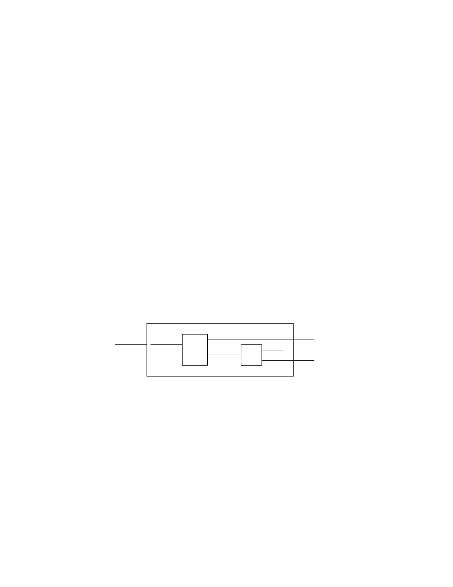
Computers

For most people today, surrounded by computers in daycares, schools, and
working places, it is quite obvious what a computer is: a digital computer
with internally stored modifiable programs. However, the meaning of the
word has changed in time. In the 1930s and 1940s (during Alan Turing’s
scientifically active period) a computer meant a person doing calculations.
Also the idea of storing programs in just the same way as data was not
at all obvious at that time. Builders of large electromechanical calculaters
put the program on cards or on a roll of punched paper, i.e., the machinery
should do the arithmetics and the instructions should be coded in some other
form. Even when turning to electronics (ENIAC in 1943), programs were still
thought of something quite different from numbers. A breakthrough came in
1945 with the EDVAC report by John von Neumann where the basic elements
of the stored program concept were introduced to the industry. This concept
had been discussed with the ENIAC engineers Eckert, Mauchly and others
in connection with their plans for a successor machine to the ENIAC.

Beeing a mathematician John von Neumann had become fascinated by

non-linear partial differential equations in the 1930s. The phenomena descri-
bed by these equations are baffling analytically and numerical work seemed
to him the most promising way to obtain a feeling for the behaviour of these
systems. This was a driving force for studying new possibilities of compu-
tation on electronic machines. Beeing a mathematician he most surely also
was familiar with Alan Turing’s work involving the concepts of logical design
and the universal machine. However, whether von Neumann applied Turing’s
ideas to the design of a computer is questionable. John von Neumann’s logi-
cal design of a computer became the prototype of most of its successors—the
von Neumann architecture (see Figure 11).

CPU

Arithmetic

logic

unit

Control

unit

¾ -

Input/output devices

Memory (instructions and data)

Instructions and data

Results

Figure 11: The von Neumann architecture

Almost at the same time, in 1945, Alan Turing presented a report, in-

dependent of the EDVAC proposel, concerning the design of a modern com-
puter. This work was inspired by his own 1936 concept of the universal
machine, his experiences during the war of the speed and reliability of elec-
tronics, and the realization of the inefficiency in designing different machines
for different logical processes. Turing’s 1945 conception of a computer was
not tied to numbers but for the logical manipulation of symbols of any kind.
From the start he stressed that the universal machine should be able to switch
at a moments notice from arithmetic to the algebra of group theory, to chess
playing, or to data processing. Further, he saw immediately the first ideas
of programming structure and languages. In addition, he was spurred by the
idea that the universal machine should be able to acquire and exhibit the
faculties of the human mind. In June 1948, in Manchester, the world’s first
practical realization of Turing’s computer principle was demonstrated.

Computer viruses

On November 3, 1983, the first computer virus was conceived as an experi-
ment to be presented at a weekly seminar on computer security. The concept
was introduced in the seminar by Fred Cohen and in 1986 he presented his
PhD Thesis [1] covering this subject. However, computer viruses can trace
their ancestor to John von Neumann’s studies of self-replicating mathemati-
cal automata in the 1940s.

For an informal first introduction of the concept of a computer virus the

analogy from the biological world is useful. A biological virus attach itself
to a cell and inserts a bit of biological ”code” into the cell so that the virus
will be reproduced and spread by that particular cell. In a computer the
cells are represented by executable files, i.e., compiled programs in machine
code. What computer viruses do is to insert themselves into executable files.
When such a file later on is running the virus can do annoying things on the
computer and it can spread itself to other executable files.

In Section 4.1 below a formal definition of a virus in connection to Turing

machines will be given. For this definition the concept of viral sets is essential.

4.1

Viral sets

By using the definitions in Section 2, the concept of the viral set can be
defined.

4.1.1

Definition

Definition 4.1 The viral set V S = {(M, V )|M is a T uring machine, V ∈
T S f or M, and ∀v ∈ V, v

⇒ V }.

Another definition that will be used frequently below is the definition of viral
sets with respect to Turing machines.

Definition 4.2 V is a viral set with respect to a Turing machine M iff (M,V)
∈ VS.

A virus can now be defined as a member of a viral set, V , with respect to a
Turing machine M.

Definition 4.3 v is a virus with respect to a Turing machine M, if v ∈ V
and (M,V) ∈ VS.

The following quotation from Cohen’s thesis [1] is illustrative.

The sequence of tape symbols we call ”viruses” is a function

of the machine on which they are to be interpreted. In particular,
we may expect that a given sequence of symbols may be a ”virus”
when interpreted by one TM and not a ”virus” when interpreted
by another TM.

According to Cohen [1] several previous attempts at definition failed be-

cause the idea of a singleton virus makes the understanding of evolution of
viruses very difficult. And evolution is indeed a central concept.

4.1.2

Evolution of viruses

A number of definitions concerning evolution of viruses will now follow.

Definition 4.4 v evolves into v

for a Turing machine M iff v and v

are

viruses and v

⇒ {v

Definition 4.5 v

is evolved from v for a Turing machine M iff v evolves

into v

for M.

Definition 4.6 v

is an evolution of v for a Turing machine M iff (M, V ) ∈

V S and ∃V

⊂ V such that ∀v

∈ V

, v

⇒ v

k+1

and ∃l, m ∈ N such that

l < m, v

= v, and v

= v

The definition above is deviating slightly from the formulation in Cohen’s
thesis [1]. However, the content should be the same. The following quotation
from Cohen’s thesis [1] summarizes the definitions above.

The ”viral set” embodies evolution by allowing elements of

such a set to produce other elements of that set as a result of
computation. So long as each ”virus” in a ”viral set” produces
some elements of that ”viral set” on some part of the tape out-
side of the original ”virus”, the set is considered ”viral”. Thus
”evolution” may be described as the production of one element
of a ”viral set” from another element of that set.

4.1.3

Basic theorems

Cohen gives a number of basic theorems concerning viral sets and these will
be repeated here without proofs. For proofs see Cohen’s thesis [1].

Theorem 4.1 Any union of viral sets is also a viral set, i.e., if (M, V

) ∈ V S

and (M, V

) ∈ V S then (M, V

∪ V

) ∈ V S.

From Theorem 4.1 it follows that the largest viral set with respect to any
machine is the union of all viral sets with respect to that machine.

For the next theorems the concept of smallest viral set has to be defined.

Definition 4.7 A smallest viral set is a viral set of which no proper subset
is a viral set with respect to the given machine. There may be many such sets
for a given machine.

Theorem 4.2 There is a machine for which the smallest viral set is a sin-
gleton set, and that the minimal viral set is therefore singleton.

It can also be shown that any sequence which duplicates itself is a virus with
respect to the machine on which it is self duplicating. These are examples
of singleton viral sets. In fact the smallest viral sets come in all sizes as the
next theorem states.

Theorem 4.3 For any finite integer i there is a machine such that there is
a smallest viral set with i elements.

4.2

Subroutines

In order to simplify the presentation of a number of proofs concerning the
computability aspects of viruses and viral detection some subroutines will

be used and they will be defined here. The subroutines will be expressed as
transition diagrams and the notation is the same as the one in Example 2.1
in Section 2.2.7.

The ”halt” subroutine will allow halting of a Turing machine in any given

state q

(see Figure 12).

¹¸

º·

∗/∗←

µ´

¶³

Figure 12: The ”halt” subroutine

The ”right till x” (or R(x)) subroutine will allow a Turing machine to

increment the position of the tape head until such a position is reached that
the symbol x is in front of the tape head (see Figure 13).

¹¸

º·

x/x→

ˆ∗/ˆ∗→

µ´

¶³

¹¸

º·

n+1

∗/∗←

¹¸

º·

n+2

Figure 13: The ”right till x” subroutine (ˆ

∗ denotes all symbols except x)

The ”left till x” (or L(x)) subroutine is just like the R(x) subroutine

except that the tape head is moving left rather than right (see Figure 14).

¹¸

º·

x/x→

ˆ∗/ˆ∗←

µ´

¶³

¹¸

º·

n+1

∗/∗←

¹¸

º·

n+2

Figure 14: The ”left till x” subroutine (ˆ

∗ denotes all symbols except x)

The next subroutine to be discussed, the ”copy from x till y after z” (or
CP Y (x, y, z)), is essential when discussing viruses. It is more complex than
the other subroutines discussed since the number of states depends on the
number of input symbols for the machine under consideration. See the loop
starting and ending in state q

n+13

in Figure 15. If all input symbols get a

unique number then 7

∗

symbolizes 7 to the power of that unique number.

Another complexity is that the copy subroutine uses a ”left of tape marker”
(N) and a ”right of tape marker” (M). These symbols should not be used

as input symbols, i.e., N, M ∈ Γ but N, M ∈

/ Σ. The left of tape marker N

is used to mark where the next symbol should be read and the right of tape
marker M is used to mark where the next symbol should be written.

n+2

R(x)

x/N →

n+3

n+5

n+7

R(y)

R(z)

∗/∗←

n+12

N/x→

n+11

n+9

L(N )

n+8

z/z→

∗/M ←

y/y→

n+14

n+16

R(M )

M/y→

n+17

∗/∗←

n+18

Out

n+13

ˆ∗/N→

k+7

∗

k+7

∗

R(M )

M/ˆ∗→

k+7

∗

∗/M ←

k+7

∗

k+7

∗

L(N )

N/ˆ∗→

Figure 15: The ”copy from x till y after z” subroutine

(ˆ

∗ denotes all symbols except y and k ≥ n + 19)

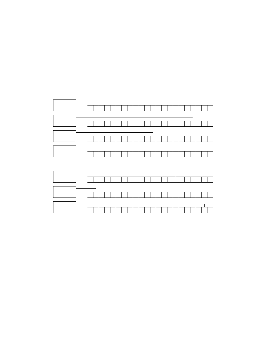
As can be seen from Figure 15, the copy subroutine makes extensive use of
the left and right subroutines. This makes sense since the tape head has to
move back and forth in order to take one symbol and copy it. The workings
of the copy subroutine may best be described using pictures and in Figure
16 a series of snapshots of a Turing machine running the subroutine is given.

· · · · · · x · · · y · · z · · · · · · · ·

n+2

· · · · · · x · · · y · · z · · · · · · · ·

n+3

· · · · · · N · · · y · · z · · · · · · · ·

n+5

· · · · · · N · · · y · · z · · · · · · · ·

n+7

· · · · · · N · · · y · · z · · · · · · · ·

n+8

· · · · · · N · · · y · · z · · · · · · · ·

n+9

· · · · · · N · · · y · · z M · · · · · · ·

n+11

· · · · · · N · · · y · · z M · · · · · · ·

n+12

· · · · · · x · · · y · · z M · · · · · · ·

n+13

· · · · · · x · · · y · · z M · · · · · · ·

k+7

· · · · · · N · · · y · · z M · · · · · · ·

k+7

· · · · · · N · · · y · · z M · · · · · · ·

k+7

· · · · · · N · · · y · · z x · · · · · · ·

k+7

· · · · · · N · · · y · · z x M · · · · · ·

k+7

· · · · · · N · · · y · · z x M · · · · · ·

n+13

· · · · · · x · · · y · · z x M · · · · · ·

n+13

· · · · · · x · · · y · · z x · · · M · · ·

n+14

· · · · · · x · · · y · · z x · · · M · · ·

n+16

· · · · · · x · · · y · · z x · · · M · · ·

n+17

· · · · · · x · · · y · · z x · · · y · · ·

n+18

· · · · · · x · · · y · · z x · · · y · · ·

Figure 16: Running of the CPY(x,y,z) subroutine

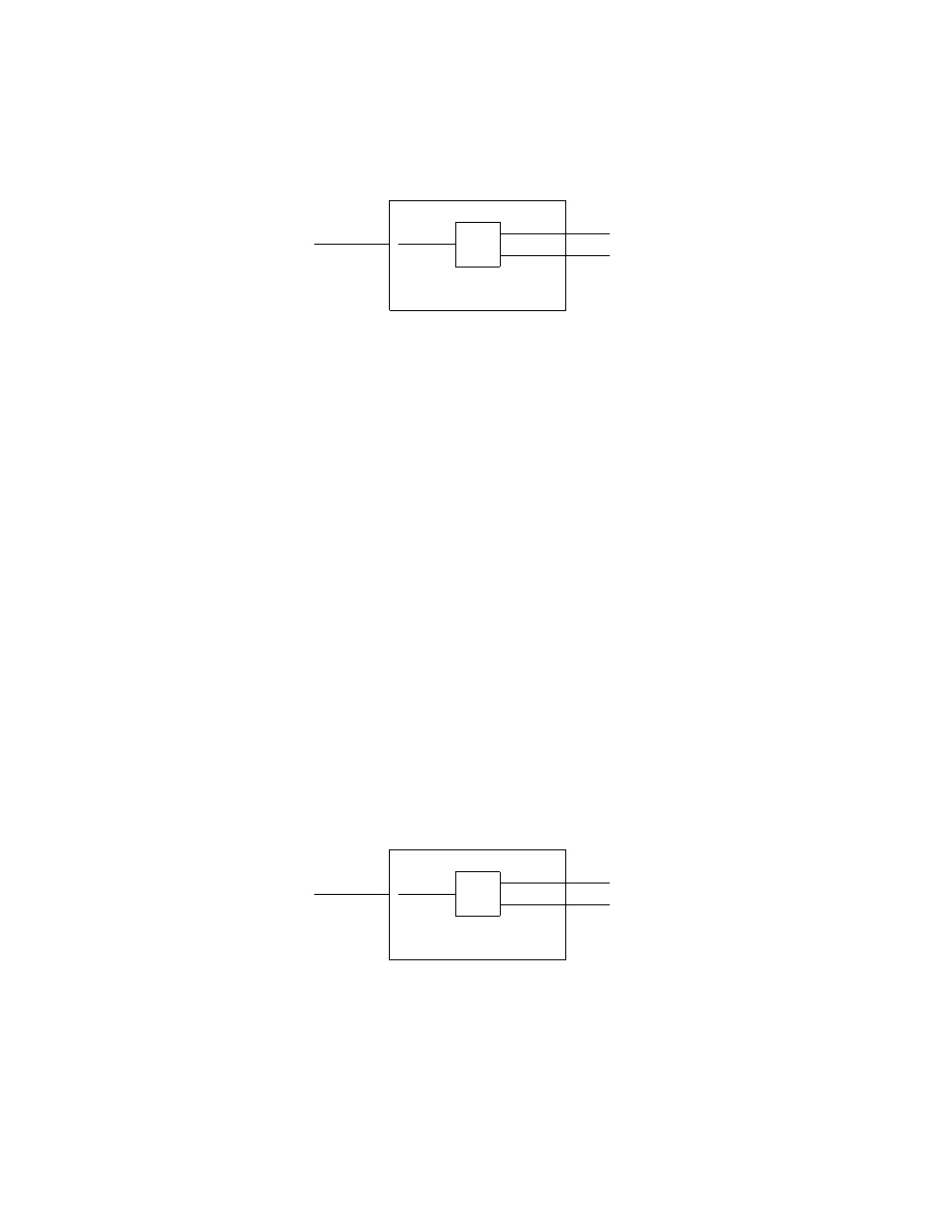
The last subroutine to be discussed is the ”generate v” (or generate(v))

subroutine. This subroutine will allow a Turing machine to generate a string
v starting from the current tape head position (see Figure 17).

¹¸

º·

∗/v

→

¹¸

º·

n+1

· · ·

n+k−1

∗/v

→

¹¸

º·

n+k

n+k+1

∗/∗←

Figure 17: The ”generate v” subroutine (v = v

· · · v

)

When the subroutines above will be used in Section 4.3 only the starting

and ending states will be shown and these will be numbered consecutively,
for instance by q

and q

, respectively. It has to be assumed that the states

in between these states are numbered differently.

4.3

Computability aspects of viruses and viral detec-
tion

In the following three subsections three issues concerning the power of viruses
will be explored. First the ”decidability” issue will be addressed. This con-
cerns the question of whether there is a Turing machine capable of determin-
ing in finite time whether or not a given sequence for a given Turing machine
is a virus. The second issue that will be addressed is the ”evolution” issue.
This concerns the question of whether there is a Turing machine capable of
determining in finite time whether or not a given virus for a given Turing
machine generates another given virus for that machine. The third and last
issue that will be addressed is the ”computability” issue. It will be shown
that any number that can be computed by a Turing machine can be evolved
by a virus, and that therefore, viruses are at least as powerful as Turing
machines as means for computation.

4.3.1

Decidability

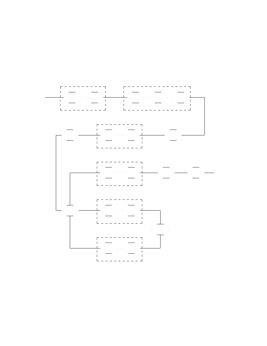
It will now be shown that it is undecidable whether or not a given (M,V)
pair belongs to the viral set. The proof below will follow the ideas in Section
2.5 and in the proof of Theorem 6 in Cohen’s thesis [1]. But the presentation
below will be somewhat simplified.

Theorem 4.4 Let VS

= {(M, {ω})|(M, {ω}) ∈ VS}. Then VS

is unde-

cidable.

Proof 4.4 In a proof by contradiction it will be assumed that VS

is decidable

and this assumption will be used to show that HALT

T M

is decidable, contra-

dicting Theorem 2.2. The key idea is to show that HALT

T M

is reducible to

Suppose that D is a decider for VS

, i.e.,

D(hM, ωi) =

accept if (M, {ω}) ∈ V S
reject if (M, {ω}) ∈/ V S.

A new Turing machine H to decide HALT

T M

, with D as a subroutine, will

now be constructed (see Figure 18).

, ω

hM, ωi

accept

reject

accept

reject

Figure 18: Turing machine H for deciding HALT

T M

The input to D is a Turing machine M, which is defined in Figure 19, and a
string ω = Llω

rR. Here it is assumed that L, l, r, R ∈

/ Σ

, that M

goes to

state q

if and only if M

halts, and that

±°

²¯

±°

²¯

l/l→, ∀q

∈ Q

ω =

Llω

accept

¹¸

º·

¹¸

º·

¹¸

º·

¹¸

º·

¹¸

º·

¹¸

º·

x+1

¹¸

º·

½¼

¾»

x+2

CPY(l,r,R)

L(l)

L(L)

CPY(L,R,R)

start

l/l→

Figure 19: Turing machine M and input string ω used in Figure 18

What M simply does is to copy ω

from inside of ω, simulate the execution

of M

on the copy of ω

, and if M

halts replicate ω. Thus M replicates ω if

and only if M

halts on input ω

. This will work since the assumptions made

above will not allow M

to corrupt the string ω and L is only found in string

ω. In order to increase the understanding of the workings of M, the running
of ω on M is given in Figure 20.

· L l ω

· · · ω

r R · · · · · · · · · · ·

· L l ω

· · · ω

r R l ω

· · · ω

r · · ·

· L l ω

· · · ω

r R l ω

· · · ω

r · · ·

· L l ω

· · · ω

r R l ω

· · · ω

r · · ·

· L l ω

· · · ω

r R l · · · · · · · · · ·

x+1

· L l ω

· · · ω

r R l · · · · · · · · · ·

x+2

· L l ω

· · · ω

r R L l ω

· · · ω

r R ·

Figure 20: Running of Llω

rR on M

Q.E.D.

Now when having proved VS

undecidable it is a simple task to prove that

VS is undecidable by simply reducing VS

to VS.

Theorem 4.5 VS is undecidable.

Proof 4.5 In a proof by contradiction it will be assumed that VS is decidable
and this assumption will be used to show that VS

is decidable, contradicting

Theorem 4.4. The key idea is to show that VS

is reducible to VS.

Suppose that D is a decider for VS, i.e.,

D(hM, V i) =

accept if (M, V ) ∈ V S
reject if (M, V ) ∈/ V S.

A new Turing machine V to decide VS

, with D as a subroutine, will now be

constructed (see Figure 21).

hM, ωi

hM, {ω}i

accept

reject

accept

reject

Figure 21: Turing machine V for deciding VS

Q.E.D.

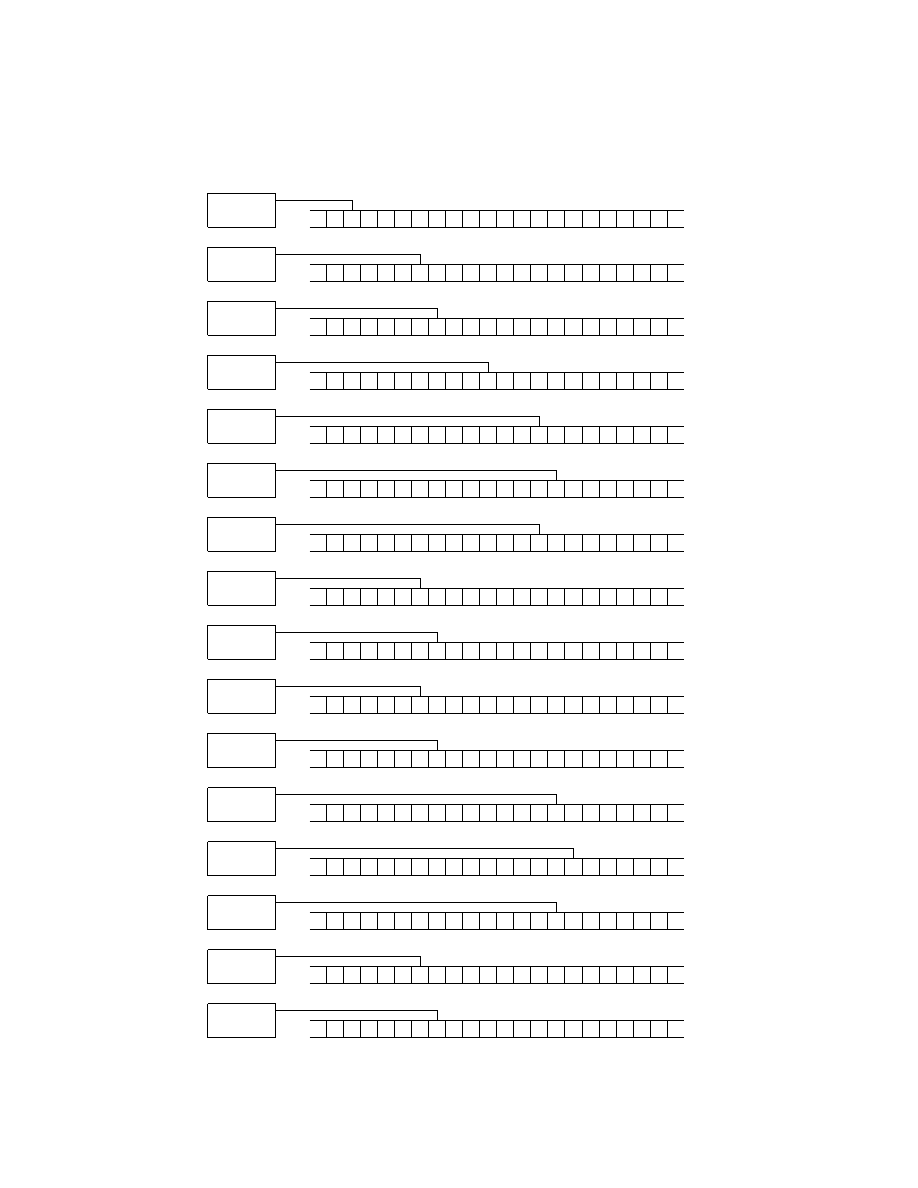
4.3.2

Evolution

It will now be shown that it is undecidable whether or not a given virus v
evolves into another given virus v

for a Turing machine M. The proof will

be similar to the proof of Theorem 4.4.

Theorem 4.6 Let EV

T M

= {(M, v, v

)|v evolves into v

for Turing machine

M}. Then EV

T M

is undecidable.

Proof 4.6 In a proof by contradiction it will be assumed that EV

T M

is de-

cidable and this assumption will be used to show that HALT

T M

is decidable,

contradicting Theorem 2.2. The key idea is to show that HALT

T M

is re-

ducible to EV

T M

Suppose that D is a decider for EV

T M

, i.e.,

D(hM, v, v

i) =

(

accept if v and v

are viruses and v

⇒ {v

}

reject otherwise.

A new Turing machine H to decide HALT

T M

, with D as a subroutine, will

now be constructed (see Figure 22).

, ω

hM, v, v

accept

reject

accept

reject

Figure 22: Turing machine H for deciding HALT

T M

The input to D is a Turing machine M, which is defined in Figure 23, a string
v = Llω

rR, and a string v

which can be defined in many ways, for example

as v with a slightly different sequence ω

instead of ω

. Here it is assumed

that L, l, r, R ∈/ Σ

, that M

goes to state q

if and only if M

halts, and

that

±°

²¯

±°

²¯

l/l→, ∀q

∈ Q

v =

Llω

acc

¹¸

º·

¹¸

º·

¹¸

º·

¹¸

º·

¹¸

º·

¹¸

º·

¹¸

º·

¹¸

º·

x+1

¹¸

º·

½¼

¾»

x+2

CPY(L,R,R)

L(L)

CPY(l,r,R)

L(l)

generate(v

)

start

l/l→

Figure 23: Turing machine M and input string v used in Figure 22

What M simply does is to copy v, copy ω

from inside of v, simulate the

execution of M

on the copy of ω

, and if M

halts generate v

. The initial self-

replication forces (M, {v}) ∈ V S. If v

is defined appropriately, for example

as suggested above, then (M, {v

}) ∈ V S. Thus M evolves v into v

if and

only if M

halts on input ω

. In order to increase the understanding of the

workings of M, the running of v on M is given in Figure 24.

· L l ω

· ω

r R · · · · · · · · · · · · · ·

· L l ω

· ω

r R L l ω

· ω

r R · · · · · · ·

· L l ω

· ω

r R L l ω

· ω

r R · · · · · · ·

· L l ω

· ω

r R L l ω

· ω

r R l ω

· ω

r · ·

· L l ω

· ω

r R L l ω

· ω

r R l ω

· ω

r · ·

· L l ω

· ω

r R L l ω

· ω

r R l ω

· ω

r · ·

· L l ω

· ω

r R L l ω

· ω

r R l · · · · · ·

x+1

· L l ω

· ω

r R L l ω

· ω

r R l · · · · · ·

x+2

· L l ω

· ω

r R L l ω

· ω

r R v

· v

· · · ·

Figure 24: Running of Llω

rR on M

Q.E.D.

4.3.3

Computability

The following discussion is an interpretation of Theorem 7 in Cohen’s the-
sis [1]. Some of the notation originates from Turing’s classical paper on
computable numbers [9]. Observe that the following discussion is an inter-
pretation and might not agree with Ref. [1] and [9].

In this subsection a Turing machine M will be constructed. A class of

viruses will also be specified. A virus in the given class will be such that a
description of a Turing machine which computes a number is embedded in
it. If v ∈ V and v

∈ V are viruses in the given class, (M, V ) ∈ V S, and v

evolves into v

for the Turing machine M then if hC

i ⊂ v then ∃j ≥ i such

that hC

i ⊂ v

. Here C

, C

, . . . , C

, . . . C

, . . . is the configuration history

for the embedded Turing machine, and will essentially contain the, so far,
computed number. If hC

i ⊂ v and hC

i+1

i ⊂ v

then v and v

are successive

members of the viral set. The successive members are called evolutions of the
previous members, and thus any number that can be computed by a Turing
machine can be evolved by a virus. Cohen [1] makes the following conclusion.

We therefore conclude that ”viruses” are at least as power-

ful a class of computing machines as TMs, and that there is a
”Universal Viral Machine” which can evolve any ”computable”
number.

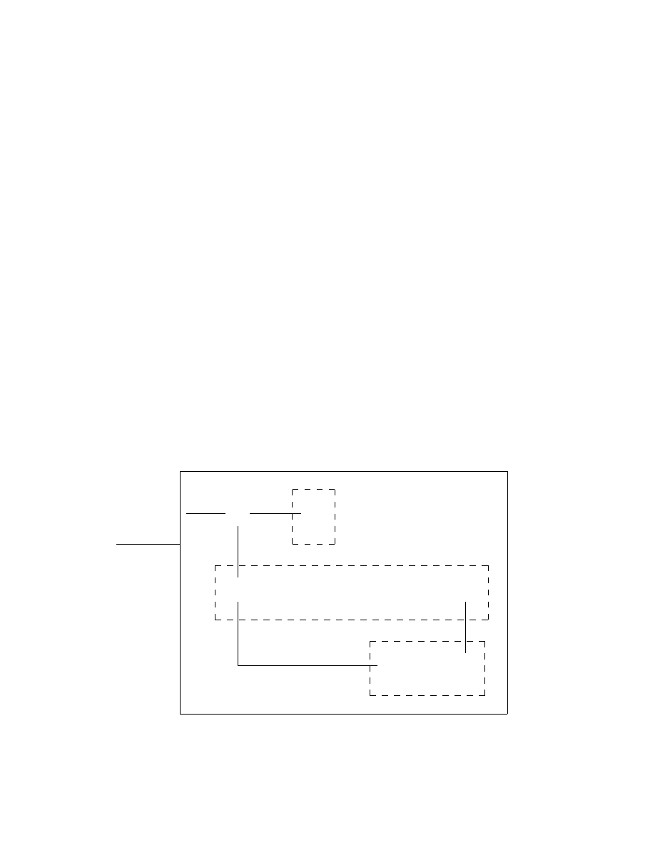
v =

LhM

i : hC

¹¸

º·

start

ˆ∗/ˆ∗←

¹¸

º·

−1

halt

¹¸

º·

L/L→

L(L)

¹¸

º·

CPY(L,R,R)

¹¸

º·

000

L(:)

¹¸

º·

0000

: / :→

¹¸

º·

∗/∗←

¹¸

º·

anf

Figure 25: Turing machine M (a possible ”Universal Viral Machine”)

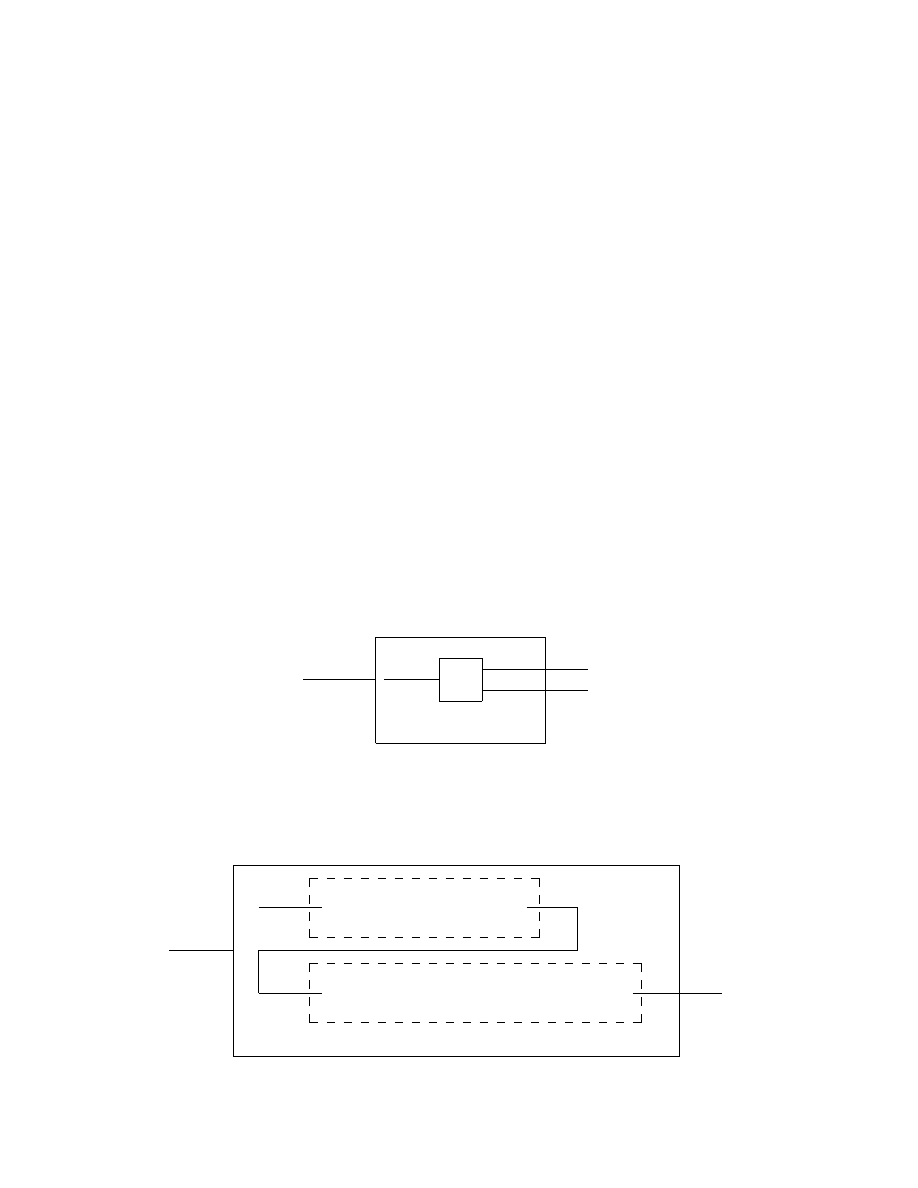
Now the Turing machine M in Figure 25 will be discussed. The input string
is a virus starting with L and ending with R. If the input string does not start

with L the machine will halt. Otherwise a copy of the virus will be written
next to the original virus, to make sure that the virus really is a virus. Apart
from L and R the input string contains a description of a Turing machine M

that computes a number, a colon, and a description of a configuration of M

Observe that no input is required for M

and the starting configuration of

is simply the start state of that machine. After the copying of the input

virus has been made the tape head is moved to the colon of the copied virus.
From there on the universal computing machine (denoted U in Figure 25) is
operating. For a description of that, see Ref. [9]. Without getting involved
in too many details it can be assumed that U by using the description of a
Turing machine and by using the description of a configuration calculates the
next configuration and replaces the old one with that. To ensure that the
right end of the virus will not be overwritten U has to be modified so that
∀q ∈ Q

and for the scanned symbol equal to R, move right 1 step, write R

on the tape, move left one step, and continue as before. Otherwise, L and
R will not be used by U. When U is finished the process of copying etc.
will start all over again, resulting in the successive members of the original
input virus on the tape. In Figure 26 the running of LhM

i : hC

iR on M is

demonstrated.

· L

R · · · · · · · · · · · ·

· L

R · · · · · · · · · · · ·

· L

R · · · · · · · · · · · ·

000

· L

R L

R · · ·

0000

· L

R L

R · · ·

anf

· L

R L

R · · ·

· L

R L

R · · ·

Figure 26: Running of LhM

i : hC

iR on M (n = i + 1)

Summary

In this paper the necessary terminology for a formal discussion of computer
viruses has been introduced. Informally a computer virus is defined as a
computer program that has the ability to infect other programs by modifying
them to include a, possibly evolved, copy of itself. Thus, every program
that gets infected may also act as a virus and infect other programs. With
the infection property, a virus can spread throughout a computer system or
network.

The following pseudo-program from Cohen’s thesis [1] shows how a virus

might be written in a pseudo-computer language.

program virus :=

{1234567;

subroutine infect-executable :=

{loop:

file = get-random-executable-file;

if first-line-of-file = 1234567

then goto loop;

prepend virus to file;}

subroutine do-damage :=

{whatever damage is to be done}

subroutine trigger-pulled :=

{return true if some condition holds}

main-program :=

{infect-executable;

if trigger-pulled then do-damage;

goto next;}

next:}

Figure 27: A simple virus

The example virus in Figure 27 searches for an uninfected executable file
by looking for executable files without the ”1234567” at the beginning. The
virus then prepends itself to the executable turning it to an infected file. After
that the virus checks if some triggering condition is true and does damage.
Finally, the virus executes the rest of the program it was prepended to.

As was shown in Section 4 it is in general impossible to detect viruses.

However, any particular virus can be detected by a particular detection
scheme [8]. For example, the virus in Figure 27 could easily be detected
by looking for ”1234567” as the first line of an executable file. If found the
executable would not be run and the virus would therefore not be able to

spread. The program in Figure 28 is used instead of the normal run com-
mand, and refuses to execute programs infected by the virus in Figure 27.

program new-run-command :=

{file = name-of-program-to-be-executed;

if first-line-of-file = 1234567 then

{print "the program has a virus";

exit;}

otherwise run file;}

Figure 28: Protection for the virus in Figure 27

Although it is possible to protect oneself for a particular virus, any detection
scheme can be circumvented. For example, if an attacker knew that a user
was using the program in Figure 28 as protection from viral attack, the virus
in Figure 27 could easily be substituted with a virus where the first line was
changed from ”1234567” to ”123456”. Thus it can be concluded that no
infection can exist that cannot be detected, and no detection mechanism can
exist that cannot be infected.

According to Cohen [8] a balance of coexistent viruses and defenses could

exist, such that a given virus could only do damage to a given portion of the
system, while a given protection scheme could only protect against a given
set of viruses. This picture will be somewhat more involved when evolution
is taken into account. In Figure 29 a modification of the virus in figure 27
to an evolutionary virus is given.

program evolutionary-virus :=

{ . . .

subroutine print-random-statement :=

{print random-variable-name, " = ", random-variable-name;

loop: if random-bit = 0 then

{print random-operator, random-variable-name;

goto loop;}

print semicolon;}

subroutine copy-virus-with-random-insertions :=

{loop:

copy evolutionary-virus to virus till semicolon-found;

if random-bit = 1 then print-random-statement;

if not-end-of-input-file goto loop;}

main-program :=

{copy-virus-with-random-insertions;

infect-executable;

if trigger-pulled then do-damage;

goto next;}

next:}

Figure 29: An evolutionary virus

Since all programs can evolve, the program that evolves into a difficult to
attack program would, according to Cohen, more likely survive as would a
virus that was more difficult to detect. A final quotation of Cohen [8]:

As evolution takes place, balances tend to change, with the

eventual result being unclear in all but the simplest circumstan-
ces. This has very strong analogies to biological theories of evo-
lution, and might relate well to genetic theories of diseases. Sim-
ilarly, the spread of viruses through systems might well be ana-
lyzed by using mathematical models used in the study of infec-
tious diseases.

Finally, it will be concluded that a virus need not be used for destructive

purposes. For example, a compression virus which finds uninfected executa-
bles, compresses them, and prepends itself to them, could be useful and,
acording to Cohen [1], save over 50% of the space taken up by executable
files in an average system. Upon execution, the infected program decom-
presses itself and executes normally.

References

1. Cohen F. B., Computer Viruses, PhD Thesis, 1986.

2. Cohen Fred, Computational Aspects of Computer Viruses, Computers

& Security, 8, 325–344, 1989.

3. Rogers H., Theory of Recursive Functions and Effective Computability,

MIT Press, Cambridge Massachusetts, 1987.

4. Sipser M., Introduction to the Theory of Computation, PWS Publish-

ing Company, 1996.

5. Burgin M., The Rise and Fall of the Church-Turing Thesis, http://arxiv

.org/pdf/cs.CC/0207055.

6. Hodges A., Alan Turing—a short biography, http://www.turing.org.uk

/turing/bio.

7. Hopcroft J. E., Motwani R., Ullman J. D., Introduction to Automata

Theory, Languages, and Computation, Addison-Wesley, 2001.

8. Cohen Fred, Cure of Computer Viruses, http://www.all.net/books/

virus/part4.html.

9. Turing A. M., On Computable Numbers, with an Application to the

Entscheidungsproblem, Proc. London Math. Soc., 42(2), 230–265,
1936.

Apart from the references mentioned above also a numerous amount of

web pages has provided information for this paper.

Wyszukiwarka

Podobne podstrony:
Wójcik, Marcin; Suliborski, Andrzej The Origin And Development Of Social Geography In Poland, With
Self Replicating Turing Machines and Computer Viruses
Globalization and youth nunistry Proyect Focus on Latin America by Daniel S Schipani
A Short Course on Computer Viruses
Mathematical models on computer viruses
The Norman Book on Computer Viruses
business group affiliiation and firm performance in a transition economy a focus on ownership voids
Correspondence of Roosevelt and Truman with Stalin on Lend Lease and Other Aid to the Soviet Union
Example CV 6 Functional CV focus on qualifications and skills
Turing s O machines, Searle, Penrose and the Brain
Virato, Swami Interview With Sogyal Rinpoche On The Tibetan Book Of Living And Dying (New Frontier
Neumann W D Notes on geometry and 3 manifolds, with appendices by P Norbury (web draft, 2004)(54s)
Stein Wilkeshuis M A Viking age Treaty Between Constantinople and Northern Merchants, With its Provi
Machining Ti–6Al–4V alloy with cryogenic compressed air cooling
Focus on First Certificate
Focus On Advanced English Grammar Practice (Longman 1999) IDVTC52QCYGR3CVGUDBDJUL7PJL2DXTUZVDM6KI

więcej podobnych podstron