
THE COMPLEXITY OF COOPERATION

p r i n c e t o n s t u d i e s i n c o m p l e x i t y
editors
Philip W. Anderson (Princeton University)
Joshua M. Epstein (The Brookings Institution)
Duncan K. Foley (Barnard College)
Simon A. Levin (Princeton University)
Gottfried Mayer-Kress (University of Illinois)
Other Titles in the Series
Lars-Erik Cederman, Emergent Actors in World Politics: How
States and Nations Develop and Dissolve
Forthcoming Titles
Scott Camazine, Jean-Louis Deneubourg, Nigel Franks, and
Thomas Seeley, Building Biological Superstructures: Models of
Self-Organization
James P. Crutchfield and James E. Hanson, Computational
Mechanics of Cellular Processes
Ralph W. Wittenberg, Models of Self-Organization in
Biological Development

THE COMPLEXITY OF COOPERATION
A G E N T - B A S E D M O D E L S O F
C O M P E T I T I O N A N D
C O L L A B O R A T I O N
Robert Axelrod
P R I N C E T O N U N I V E R S I T Y P R E S S
P R I N C E T O N , N E W J E R S E Y

Copyright
䉷 1997 by Princeton University Press
Published by Princeton University Press, 41 William Street,
Princeton, New Jersey 08540
In the United Kingdom: Princeton University Press, Chichester,
West Sussex
All Rights Reserved
Library of Congress Cataloging-in-Publication Data
Axelrod, Robert M.
The complexity of cooperation : agent-based models of competition
and collaboration / Robert Axelrod.
p. cm. — (Princeton studies in complexity.)
Includes bibliographical references and index.
ISBN 0-691-01568-6 (cloth : alk. paper). — ISBN 0-691-01567-8
(pbk. : alk. paper)
1. Cooperativeness. 2. Competition. 3. Conflict management.
4. Adaptability (Psychology) 5. Adjustment (Psychology)
6. Computational complexity. 7. Social systems—Computer
simulation. I. Title. II. Series.
HM131.A894 1997
302
⬘.14—dc21 97-1107 CIP
This book has been composed in Sabon
Princeton University Press books are printed
on acid-free paper and meet the guidelines
for permanence and durability of the Committee
on Production Guidelines for Book Longevity
of the Council on Library Resources
Printed in the United States of America by Princeton Academic Press
10 9 8 7 6 5 4 3 2 1
10 9 8 7 6 5 4 3 2 1
(Pbk.)

To Amy, Lily, and Vera


Contents
List of Tables and Figures
ix
Preface
xi
Introduction
3
1. Evolving New Strategies
10
2. Coping with Noise
30
3. Promoting Norms
40
4. Choosing Sides
69
5. Setting Standards
95
6. Building New Political Actors
121
7. Disseminating Culture
145
Appendixes
A. Replication of Agent-Based Models
181
B. Resources for Agent-Based Modeling
206
Index
223


Tables and Figures
Tables
1-1
The Prisoner’s Dilemma
16
1-2
The Basic Simulation
19
3-1
Example of Payoffs in the Norms Game
49
4-1
The Two Configurations Predicted for the Second
World War in Europe
85
5-1
The Two Nash Equilibrium Configurations
113
5-2
Analysis of Variation in Rivalry Parameters around the
Base Case
114
5-3
Extended Analysis of Variation in Rivalry Parameters
115
6-1
Commitments Forming a Proximity Pattern
136
6-2
Commitments Forming Pattern of Two Clusters
136
6-3
Development of Clusters of Commitments
137
7-1
A Typical Initial Set of Cultures
155
7-2
Average Number of Stable Regions
160
7-3
An Illustration of Social Influence between Dialects
164
A-1
Average Number of Stable Regions
191
A-2
Axelrod’s Work Log
199
A-3
Axtell’s Work Log
200
Figures
1-1
Prisoner’s Dilemma in an Evolving Environment
23
2-1
Performance as a Function of Noise
36
2-2
Ecological Simulation
37
3-1
Norms Game
49
3-2
Norms Game Dynamics
51
3-3
Metanorms Game
53
3-4
Metanorms Game Dynamics
54
4-1
A Landscape with Two Local Optima
77
6-1
Wealth of Each Actor over 1,000 Years (Population 1)
132
6-2
Fights and Population Wealth in Population 1
133
6-3
Wealth of Each Actor over 1,000 Years (Population 2)
134

x
T A B L E S A N D F I G U R E S
6-4
Fights and Population Wealth in Population 2
134
6-5
Wealth of Each Actor over 1,000 Years
(Population 3)
135
6-6
Fights and Population Wealth in Population 3
135
6-7
Late Collapse of a Powerful Actor
138
6-8
Internal Conflict
139
7-1
Map of Cultural Similarities
157
7-2
Average Number of Stable Regions
162
7-3
Number of Cultural Regions and Cultural Zones over
Time
166
A-1
Average Number of Stable Regions in Axelrod’s
Cultural Model and Sugarscape Implementation
192

Preface
This book is a sequel to The Evolution of Cooperation (Axelrod 1984).
That book had a single paradigm and a simple theme. The paradigm was
the two-person iterated Prisoner’s Dilemma. The theme was that cooper-
ation based upon reciprocity can evolve and sustain itself even among
egoists provided there is sufficient prospect of a long-term interaction.
The theme was developed from many different angles, including
computer tournaments, historical cases, and mathematical theorems.
The two-person iterated Prisoner’s Dilemma is the E. coli of the social
sciences, allowing a very large variety of studies to be undertaken in a
common framework. It has even become a standard paradigm for study-
ing issues in fields as diverse as evolutionary biology and networked
computer systems. Its very simplicity has allowed political scientists,
economists, sociologists, philosophers, mathematicians, computer scien-
tists, evolutionary biologists, and many others to talk to each other. In-
deed, the analytic and empirical findings about the Prisoner’s Dilemma
from one field have often led to insights in other fields.
1
The Evolution of Cooperation, with its focus on the Prisoner’s Di-
lemma, was written during the Cold War. Indeed, one of its primary mo-
tivations was to help promote cooperation between the two sides of a
bipolar world. My hope was that a deeper understanding of the condi-
tions that promote cooperation could help make the world a little safer.
The work was well received in academic circles, and even among scholars
interested in policy-relevant research.
2
Nevertheless, I was keenly aware
that there was much more to cooperation than could be captured by any
single model, no matter how broad its applications or how rich its strate-
gic implications.
The present book is based on a series of studies that go beyond the
basic paradigm of the Prisoner’s Dilemma. It includes an analysis of strat-
egies that evolve automatically, rather than by human invention. It also
considers strategies designed to cope with the possibility of misunder-
standings between the players or misimplementation of a choice. It then
expands the basis of cooperation to more than a choice with a short-run
cost and a possible long-run gain. It includes collaboration with others to
1
For reviews, see Axelrod and Dion (1988) and Axelrod and D’Ambrosio (1995).
2
For example, in 1990 I received the National Academy of Sciences’ new Award for
Behavioral Research Relevant to the Prevention of Nuclear War. On the Soviet side, several
senior defense intellectuals and scientists involved in arms-control policy reported that they
read the book with interest, and had passed it around to their friends.

xii
P R E F A C E
build and enforce norms of conduct, to win a war or to impose an indus-
trial standard, to build a new organization that can act on behalf of its
members, and to construct a shared culture based on mutual influence.
Expansion of the potential forms of collaboration implies the expan-
sion of the potential forms of competition. The present volume therefore
considers more than whether or not two players cooperate. It includes
the conflicts between violators and enforcers of a norm, the threats and
wars among nations, competition among companies, contests among or-
ganizations for wealth and membership, and competing pulls of social
influence for cultural change.
This book includes work done from 1986 to 1996, a period in which
the Cold War was coming to an end and a new era was taking shape. My
own research agenda was deeply affected by these dramatic and unex-
pected transformations. The transformations of this decade were espe-
cially salient because during this period I was fortunate to have had op-
portunities to participate in international activities aimed at promoting
cooperation, first between the United States and the Soviet Union, and
then among the various warring groups in the former Yugoslavia. It is
ironic that my theoretical work on two-person games led to my participa-
tion in international activities just as the bi-power world of the Cold War
was coming to an end.
In 1986, I joined a committee of the National Academy of Sciences
examining the relevance of behavioral and social sciences to the preven-
tion of nuclear war. Among other projects, this committee promoted par-
allel and collaborative research with Soviet scholars on topics of mutual
interest.
My participation in this committee also led to my joining a second
committee of the National Academy of Sciences, the Committee on Inter-
national Security and Arms Control. This committee consisted mostly of
physical scientists and worked with a counterpart Soviet group. Our mis-
sion was to consider fruitful avenues for arms-control initiatives that
would go beyond what was currently being negotiated between the two
governments. Among the members were scientists with decades of expe-
rience in arms control and a former Chairman of the Joint Chiefs of Staff.
The Soviet counterpart committee included several key science advisors
to the Soviet leader, Mikhail Gorbachev.
Participating in these social science and arms-control forums taught
me a great deal about how international politics was viewed by leading
scholars and policy activists. In particular, I was impressed by the intel-
lectual efforts of leading thinkers on both sides to formulate concepts and
recommendations that would capitalize on the new opportunities of the
era as well as deal with the new dangers of instability. The difficulties
faced by these talented, experienced, and practical leaders reinforced my

P R E F A C E
xiii
own faith in the potential value of research into fundamental political
and social processes.
I was also affected by what was happening outside our committee
meetings. Our work brought me to meetings in Uzbekistan in 1988 and
Estonia in 1989, as well as Russia. In Estonia, I asked our Soviet hosts if
they could find a way for us to meet with both the Estonian nationalists,
who were then accelerating their demands for independence, and the eth-
nic Russians who opposed them. Having them meet in one room was
impossible, I was politely told, but separate meetings were arranged for
our benefit. This gave me a firsthand feel for the depth of nationalist
sentiment and heightened my interest in cultural conflict and nationalism
as fundamental forces in the world. These interests in turn led to work
included in this book on how new political actors are formed and how
social influence promotes cultural change as the foundation of political
change.
In 1989, however, I accepted the validity of the quip that if it came to a
conflict between Estonia and Moscow, the winner would be the Red
Army. Yet within two years the Soviet Union had collapsed and Estonia
as well as all the other republics had their independence.
As democracy was developing in Russia, Yugoslavia disintegrated. In
Bosnia, a bitter civil war ensued, marked by a level of atrocities not seen
in Europe for fifty years. At the height of the fighting, in the summer of
1995, I was invited by the United Nations to talk about my work on
cooperation at a conference designed to bring together nongovernmental
representatives of all the warring factions in the former Yugoslavia. The
participants had many critical questions about how my Prisoner’s Di-
lemma work applied to the complexity of their conflicts, with its unequal
power, with fifteen rather than two sides to the conflicts, and with viola-
tions of widely held norms of conduct.
Many of the issues raised by the participants did not have simple an-
swers, but they were ones on which I had been actively working. The
present volume includes models that deal with unequal power, with mul-
tisided as well as two-sided conflict, with misunderstandings and mis-
implementions, with the enforcement of norms, with newly emerging po-
litical entities, and with the cultural basis for political affiliation and
polarization. Although I have no solutions, I believe that analyzing large-
scale outcomes in terms of the interactions of actors can enhance our
understanding of conflict and cooperation in a complex world.
The seven chapters of this book were first published in journals and
edited volumes of political science, conflict studies, organizational sci-
ence, and computer science. The separate articles originally appeared in
such a wide range of places that people who may have read one or two of
them are unlikely to be aware of the others. Publishing these articles as a

xiv
P R E F A C E
collected set may be of special value to three partly overlapping groups of
readers: those who want to learn about extensions to the two-person
Prisoner’s Dilemma, those who are interested in conflict and collabora-
tion in a variety of settings, and those who are interested in agent-based
modeling in the social sciences.
To place the work in a wider context, I have added a variety of new
material:
1. An introductory chapter describing the common themes of the volume
and showing how the individual chapters relate to each other.
2. Introductory material for each chapter showing how it grew out of my
long-term interests, recounting experiences related to the project, and describ-
ing how the work was received.
3. An appendix providing resources for students and scholars who wish to
do their own agent-based modeling.
With the supplementary material, the volume should be accessible to
an advanced undergraduate interested in fundamental aspects of political
and social change. Readers unfamiliar with the iterated Prisoner’s Di-
lemma may wish to consult any standard game-theory text, or Axelrod
(1984, 1–15). In the few places where specialized knowledge is used, the
argument is also explained in simpler terms.
I acknowledge with pleasure the encouragement and helpful criticism
of the BACH research group: Arthur Burks, Michael Cohen, John Hol-
land, Rick Riolo, and Carl Simon. It has been an education, a joy, and an
honor to have been part of the BACH group for well over a decade. For
editorial help with this volume, I would like to thank Amy Saldinger. For
the index I thank Lisa D’Ambrosio. I would also like to thank all those
people and institutions who helped with chapters of this book. Their
names are given in the appropriate places. Finally, for financial help in
completing this book, I would like to thank the Defense Advanced Proj-
ect Research Agency for its assistance through the Santa Fe Institute, and
the University of Michigan for its assistance through both the LS&A
College Enrichment Fund and the School of Public Policy.
References
Axelrod, Robert. 1984. The Evolution of Cooperation. New York: Basic Books.
Axelrod, Robert, and Lisa D’Ambrosio. 1995. “Announcement for Bibliography
on the Evolution of Cooperation.” Journal of Conflict Resolution 39:190.
Axelrod, Robert, and Douglas Dion. 1988. “The Further Evolution of Coopera-
tion.” Science 242 (9 Dec.):1385–90.

THE COMPLEXITY OF COOPERATION


Introduction
The title of this book illustrates the dual purposes of the volume. One
meaning of “The Complexity of Cooperation” refers to the addition of
complexity to the most common framework for studying cooperation,
namely the two-person iterated Prisoner’s Dilemma. Adding complexity
to that framework allows the exploration of many interesting and impor-
tant features of competition and collaboration that are beyond the reach
of the Prisoner’s Dilemma paradigm.
The second meaning of “The Complexity of Cooperation” refers to the
use of concepts and techniques that have come to be called complexity
theory. Complexity theory involves the study of many actors and their
interactions. The actors may be atoms, fish, people, organizations, or
nations. Their interactions may consist of attraction, combat, mating,
communication, trade, partnership, or rivalry. Because the study of large
numbers of actors with changing patterns of interactions often gets too
difficult for a mathematical solution, a primary research tool of complex-
ity theory is computer simulation. The trick is to specify how the agents
interact, and then observe properties that occur at the level of the whole
society. For example, with given rules about actors and their interactions,
do the actors tend to align into two competing groups? Do particular
strategies dominate the population? Do clear patterns of behavior
develop?
The simulation of agents and their interactions is known by several
names, including agent-based modeling, bottom-up modeling, and artifi-
cial social systems. Whatever name is used, the purpose of agent-based
modeling is to understand properties of complex social systems through
the analysis of simulations. This method of doing science can be con-
trasted with the two standard methods of induction and deduction. In-
duction is the discovery of patterns in empirical data.
1
For example, in
the social sciences induction is widely used in the analysis of opinion
surveys and macroeconomic data. Deduction, on the other hand, in-
volves specifying a set of axioms and proving consequences that can be
derived from those assumptions. The discovery of equilibrium results
in game theory using rational-choice axioms is a good example of
deduction.
Agent-based modeling is a third way of doing science. Like deduction,
it starts with a set of explicit assumptions. But unlike deduction, it does
1
Induction as a search for patterns in data should not be confused with mathematical
induction, which is a technique for proving theorems.

4
I N T R O D U C T I O N
not prove theorems. Instead, an agent-based model generates simulated
data that can be analyzed inductively. Unlike typical induction, however,
the simulated data come from a rigorously specified set of rules rather
than direct measurement of the real world. Whereas the purpose of in-
duction is to find patterns in data and that of deduction is to find conse-
quences of assumptions, the purpose of agent-based modeling is to aid
intuition.
Agent-based modeling is a way of doing thought experiments. Al-
though the assumptions may be simple, the consequences may not be at
all obvious. Numerous examples appear throughout this volume of lo-
cally interacting agents producing large-scale effects. The large-scale ef-
fects of locally interacting agents are called “emergent properties” of the
system. Emergent properties are often surprising because it can be hard
to anticipate the full consequences of even simple forms of interaction.
2
There are some models, however, in which emergent properties can be
formally deduced. Good examples include the neoclassical economic
models in which rational agents operating under powerful assumptions
about the availability of information and the capability of optimizing can
achieve an efficient reallocation of resources among themselves through
costless trading. But when the agents use adaptive rather than optimizing
strategies, deducing the consequences is often impossible; simulation be-
comes necessary.
Throughout the social sciences today, the dominant form of modeling
is based upon the rational-choice paradigm. Game theory, in particular, is
typically based upon the assumption of rational choice. In my view, the
reason for the dominance of the rational-choice approach is not that
scholars think it is realistic. Nor is game theory used solely because it
offers good advice to a decision maker, because its unrealistic assump-
tions undermine much of its value as a basis for advice. The real advan-
tage of the rational-choice assumption is that it often allows deduction.
The main alternative to the assumption of rational choice is some form
of adaptive behavior. The adaptation may be at the individual level
through learning, or it may be at the population level through differential
survival and reproduction of the more successful individuals. Either way,
the consequences of adaptive processes are often very hard to deduce
when there are many interacting agents following rules that have non-
linear effects. Thus the simulation of an agent-based model is often the
only viable way to study populations of agents who are adaptive rather
than fully rational.
Although agent-based modeling employs simulation, it does not aim to
2
Some complexity theorists consider surprise to be part of the definition of emergence,
but this raises the question of surprising to whom?

I N T R O D U C T I O N
5
provide an accurate representation of a particular empirical application.
Instead, the goal of agent-based modeling is to enrich our understanding
of fundamental processes that may appear in a variety of applications.
This requires adhering to the KISS principle, which stands for the army
slogan “keep it simple, stupid.”
The KISS principle is vital because of the character of the research
community. Both the researcher and the audience have limited cognitive
ability. When a surprising result occurs, it is very helpful to be confident
that we can understand everything that went into the model. Although
the topic being investigated may be complicated, the assumptions under-
lying the agent-based model should be simple. The complexity of agent-
based modeling should be in the simulated results, not in the assumptions
of the model.
Of course there are many other uses of computer simulation in which
the faithful reproduction of a particular setting is important. A simula-
tion of the economy aimed at predicting interest rates three months into
the future needs to be as accurate as possible. For this purpose the as-
sumptions that go into the model may need to be quite complicated.
Likewise, if a simulation is used to train the crew of a supertanker or to
develop tactics for a new fighter aircraft, accuracy is important and sim-
plicity of the model is not. But if the goal is to deepen our understanding
of some fundamental process, then simplicity of the assumptions is im-
portant, and realistic representation of all the details of a particular set-
ting is not.
My earlier work on the Prisoner’s Dilemma (Axelrod 1984) illustrates
this theme. My main motivation for learning about effective strategies
was to find out how cooperation could be promoted in international poli-
tics, especially between the East and the West during the Cold War. As it
happened, my tournament approach and the evolutionary analysis that
grew out of it suggested applications of which I had not even dreamed.
For example, controlled experiments show that stickleback fish use the
tit for tat strategy to achieve cooperation based upon reciprocity (Mil-
inski 1987).
At a political science convention, a colleague came up to me and said
she really appreciated my work and found it helpful for her divorce. She
explained that my book showed her that she had been a sucker during
her marriage, always giving in to her husband. I asked whether the book
helped save her marriage. “No,” she replied. “I didn’t want to save my
marriage. But it certainly helped with the divorce settlement. I started to
play tit for tat, and once he learned that I couldn’t be pushed around, I
got a much better deal.”
The fact that a single model, in this case the Prisoner’s Dilemma, can be
useful in understanding the dynamics between foraging fish and between

6
I N T R O D U C T I O N
divorcing people is not due to the accuracy of the model in representing
the details of either situation. Instead it is due to the fact that an ex-
tremely simple model captures a fundamental feature of many interac-
tions. What the Prisoner’s Dilemma captures so well is the tension be-
tween the advantages of selfishness in the short run versus the need to
elicit cooperation from the other player to be successful in the longer run.
The very simplicity of the Prisoner’s Dilemma is highly valuable in help-
ing us to discover and appreciate the deep consequences of the funda-
mental processes involved in dealing with this tension.
A moral of the story is that models that aim to explore fundamental
processes should be judged by their fruitfulness, not by their accuracy.
For this purpose, realistic representation of many details is unnecessary
and even counterproductive. The models presented in the volume follow
this same logic of simplicity. The intention is to explore fundamental
social processes. Although a particular application may have motivated a
given model, the primary aim is to undertake the exploration in a manner
so general that many possible settings could be illuminated.
Taken as a whole, this book presents a set of studies that are unified in
three ways. First, they all deal with problems and opportunities of coop-
eration in a more or less competitive environment. Second, they all em-
ploy models that use adaptive rather than rational agents. Although
people may try to be rational, they can rarely meet the requirements of
information or foresight that rational models impose (Simon 1955;
March 1978). Third, they all use computer simulation to study the emer-
gent properties of the interactions among the agents. Thus they are all
agent-based models. The simulation is necessary because the interactions
of adaptive agents typically lead to nonlinear effects that are not amen-
able to the deductive tools of formal mathematics.
The chapters can be read either separately or as a whole. The order of
the presentation represents a progression from variations on the Pris-
oner’s Dilemma paradigm (Chapters 1 and 2), to different strategic
models (Chapters 3, 4, and 5), to an examination of the emergence of
new political actors and shared culture (Chapters 6 and 7). The order of
the chapters is also the order in which I did the work, with the exception
that Chapter 2 represents later work on an earlier theme.
The first project represents my effort to go beyond the tournament
approach to generating a rich strategic environment. The tournament
approach solicited entries from professionals and amateurs, each trying
to develop a strategy for the Prisoner’s Dilemma that would do well in
the environment provided by all the submissions. Having done two
rounds of the tournament, I wondered whether the amount of coopera-
tion I observed was due to the prior expectations of the people who sub-
mitted the rules. Fortunately, a colleague, John Holland, had developed

I N T R O D U C T I O N
7
an automated method for evolving a population of strategies from a ran-
dom start. The technique is called the genetic algorithm. I tried it, and it
performed far beyond my expectations. The results are in Chapter 1.
An important extension of the basic Prisoner’s Dilemma is consider-
ation of what happens when a player might misunderstand what the
other did on the previous move or might fail to implement the intended
choice. These kinds of “noise” can have a big impact on the performance
of a given strategy, and hence on the best means of attaining cooperation
among egoists. Several suggestions had been proposed in the literature
for dealing with noise, including adding generosity or contrition to reci-
procity, as well as a completely different strategy based upon learning
through reward and punishment. I wanted to see how these different
approaches would work in a noisy environment. A postdoctoral visitor
from China, Wu Jianzhong, and I found that generous or contrite ver-
sions of the classic tit for tat strategy did very well in a variegated
noisy environment, even better than the Pavlovian strategy. Chapter 2
explains how these strategies performed and why.
For a long time, I had been eager to move beyond the two-person
format of the basic Prisoner’s Dilemma. I especially wanted to find out
how cooperation could emerge when many people interacted with each
other in groups rather than in pairs. It was well known that the straight-
forward extension of the Prisoner’s Dilemma to an n-person version will
not sustain cooperation very well because the players have no way of
focusing their punishment on someone in the group who has failed to
cooperate. Nevertheless, social norms do emerge and are often quite
powerful means of sustaining cooperation. So I developed a “norms
game” that allowed players to punish individuals who do not cooperate.
It turned out that another twist was needed lest all the cooperators be
tempted to let someone else be the one to bear the costs of disciplining the
noncooperators. This led to a wide-ranging study of the mechanisms for
promoting norms (Chapter 3).
Another form of cooperation occurs when people organize themselves
into groups to compete with each other. This is clearly an example of
collaboration in the interests of competition. It takes place in many
forms, including alliances among nations, strategic partnerships among
businesses, and coalitions among political parties in parliamentary de-
mocracies. Having worked on the problem of coalition formation in Italy
as part of my dissertation in the late 1960’s, I was struck by how political
parties wanted to work with others who were similar to themselves (Ax-
elrod 1970). Two decades later, I returned to this theme of choosing sides
based upon affinity rather than strategic advantage. Working with a
graduate student, Scott Bennett, I developed a model for how players
choose sides. We found that the model actually did a good job of ac-

8
I N T R O D U C T I O N
counting for how European countries were aligned in World War II
(Chapter 4).
The same model even worked well in accounting for how computer
companies took sides in the competition to develop standards for the
UNIX operating system (Chapter 5). This was work done with Scott Ben-
nett and three collaborators from the Michigan Business School: Will
Mitchell, Robert E. Thomas, and Erhard Bruderer.
An even deeper problem is how independent actors sometimes cooper-
ate to such an extent that they give up most of their independence. The
result is a new level of organization that behaves as an independent actor in
its own right. Multicellular organisms evolved this way, and so have many
large business organizations. My approach to analyzing how new levels of
political actors can arise uses a model of war, threats, and commitments.
The agent-based model and its results are provided in Chapter 6.
Whereas the model in Chapter 6 attributes the emergence of new ac-
tors to the dynamics of coping with conflict, I also wanted to study an
even more fundamental question: how people become more alike so that
they find it easier to work together in the first place. This led to a study of
the process of social influence and the emergence of shared culture. Once
again, the transformations of the post-Cold War environment helped em-
phasize the importance of returning to some very fundamental issues
about the basis for cooperation within as well as between societies. The
resulting model of social influence and cultural change is given in Chap-
ter 7.
Two appendixes provide supporting material about agent-based mod-
eling. Appendix A develops the concepts and methods of comparing
agent-based models through a process called “alignment.” Alignment is
needed to determine whether two modeling systems can produce the
same results, which in turn is the basis for critical experiments and for
tests of whether one model can subsume another. The work provides a
case study of alignment, using the model of social influence presented in
Chapter 7. The project was done with Robert Axtell, Joshua Epstein, and
Michael Cohen. Appendix B provides resources for students and scholars
who wish to do their own agent-based modeling. It includes advice on
programming such models, exercises to develop one’s skills, and sug-
gested readings for applications of complexity theory and agent-based
modeling to the social sciences.
Associated with this volume is an Internet site.
3
The site includes the
source code and documentation for most of the models in this book. It
also provides links to many topics related to complexity theory, agent-
based modeling, and cooperation.
3
http:/ /pscs.physics.lsa.umich.edu/Software/ComplexCoop.html

I N T R O D U C T I O N
9
References
Axelrod, Robert. 1970. Conflict of Interest. Chicago: Markham.
. 1984. The Evolution of Cooperation. New York: Basic Books.
March, James G. 1978. “Bounded Rationality, Ambiguity and the Engineering of
Choice.” Bell Journal of Economics 9: 587–608.
Milinski, Manfred. 1987. “tit for tat in Sticklebacks and the Evolution of Co-
operation.” Nature 23: 434–35.
Simon, Herbert A. 1955. “A Behavioral Model of Rational Choice.” Quarterly
Journal of Economics 69: 99–118.

1
Evolving New Strategies
This chapter began with a hammer and a nail. The nail was a problem I
wanted to solve. The hammer was a tool I wanted to try out that looked
well suited to driving my nail. The problematic nail was the question of
whether the success of the tit for tat strategy in my computer tourna-
ments depended in large part on the prior beliefs of the people who sub-
mitted strategies about what the other submissions would be like. In
other words, would the tournament results be influenced by what people
believed others would be doing, or would something like the reciprocity
of tit for tat succeed in a tournament setting without any preconcep-
tions about the tendencies or even the responsiveness of others?
Answering this question would require a method of generating new
strategies that would not involve human preconceptions. A tool for doing
precisely this was developed by John Holland, a computer scientist at
Michigan. I knew John well from a small research group we were both
part of for years. This was the BACH group, named after its original
members: Arthur Burks, myself, Michael Cohen, and John Holland.
John’s genetic algorithm technique (Holland 1975) was inspired by the
ability of evolution to discover adaptive solutions to hard problems. By
the mid-1980’s, the genetic algorithm had proven to be an effective
search technique for discovering effective solutions in highly complex
computer problems (Goldberg 1989; Mitchell 1996).
My own interest in evolutionary simulation dates back to 1960, when I
did a high school science project on computer simulation of hypothetical
life forms and environments. At the University of Chicago I was a math
major, but also spent a summer with the Committee on Mathematical
Biology reading about evolutionary biology. Despite these interests in
computers, mathematics, and evolution, I chose to go to graduate school
in political science. The problems I most wanted to work on dealt with
the prevention of conflict between nations, especially nuclear war. After
getting my Ph.D. from Yale, I taught international politics at Berkeley
and then moved to the University of Michigan, where I took a joint ap-
pointment in the Department of Political Science and what is now the
School of Public Policy.
At Michigan, Michael Cohen became my closest colleague. He kept
suggesting that I meet John Holland and learn about his work. Eventu-
ally I succumbed—to my great joy and benefit. Among other things, I

E V O L V I N G N E W S T R A T E G I E S
11
learned about the potential of John’s genetic algorithm as a method of
discovering highly adaptive responses even in complicated contexts. So
when I had the nail of needing to study the evolution of Prisoner’s Di-
lemma strategies and the hammer of the genetic algorithm, it seemed like
a perfect match.
The first thing I did was to test the genetic algorithm to see if it could
perform well in an environment I thought I knew fairly well, namely, the
rules submitted to the second round of my tournament. The algorithm
performed beyond my wildest expectations, evolving strategies that were
more effective than what I thought was even possible in this environ-
ment. Having convinced myself that this was indeed a hammer that could
pound my kind of nails, I next used it on my real problem. I started with
a population of strictly random strategies (chosen from a huge universe
of possible strategies that had no bias toward either cooperation or reci-
procity), and let the population evolve using the genetic algorithm.
Within a very short time, the population evolved toward strategies that
behaved very much like tit for tat, and were certainly achieving coop-
eration based upon reciprocity. This demonstrated that the success of
reciprocity in my two rounds of human submissions was not a fluke that
depended upon particular prior beliefs about what other submissions
would look like.
I was pleased that earlier claims about reciprocity were even more ro-
bust than I had imagined. I was also pleased because I would not have to
devote my life to conducting more and more rounds of the computer
tournament, as a number of people had requested that I do.
The resulting paper was first published as a chapter in a book on the
genetic algorithm and related computer techniques. It is widely cited in
the computer science literature on the genetic algorithm. The reason
seems to be that the Prisoner’s Dilemma provides a task that is easy to
understand, and the performance of the genetic algorithm on this task is
quite impressive. In addition, this was the first application of the genetic
algorithm to evolving strategies in an interactive setting. Unfortunately,
the appearance of this paper in a computer science collection has meant
that it has not been very accessible to social scientists.
This project has an interesting sequel that deals with the adaptive value
of sexual reproduction. The story involves William D. Hamilton, with
whom I had previously worked on biological applications of my work on
the Prisoner’s Dilemma (Axelrod and Hamilton 1981).
1
As I was com-
pleting my paper on the genetic algorithm, Bill told me about his theory
that sex was an adaptation to resist parasites. Bill is one of the world’s
leading evolutionary biologists, so when he suggested a novel theory, I
1
Our paper is also included in revised form as Chapter 5 of Axelrod (1984).

12
C H A P T E R 1
took it seriously, no matter how bizarre it sounded at first. He pointed
out that virtually all large animals and plants reproduce sexually, even
though sexual reproduction can be very costly. In mammals, for example,
the cost can be as large as two-for-one when half the adults, the males, do
not give birth. What advantage conferred by sex makes up for this huge
cost is one of the great unsolved puzzles in evolutionary biology. Bill’s
idea, roughly stated, was that all large animals and plants have the prob-
lem of resisting parasites by being able to distinguish their own cells from
parasites that evolve to fool them. Parasites, being much smaller, repro-
duce much faster than the hosts, so they can evolve faster than the hosts.
Sex, Bill reasoned, allows the offspring of the hosts to be different from
either the mother or the father, and thereby makes it hard for parasites
that have adapted well to a host to be well adapted to the host’s off-
spring. By juggling the genes of two parents, sex allows a host species to
resist its rapidly evolving parasites.
This was a fascinating idea. Bill told me, however, that he had trouble
working out a mathematical model that could be solved. The problem
was that the model would have to include many genes, but mathematical
models of genetics typically became quite unmanageable when there are
more than two interacting genes. “No problem,” I said. I had a technique
based on Holland’s genetic algorithm that could easily handle dozens of
interacting genes. Moreover, it could easily represent the competition be-
tween hosts and parasites. So Bill and I worked with a graduate computer
science student, Reiko Tanese. We adapted the genetic algorithm to test
whether sexual reproduction of the hosts could indeed overcome the
two-for-one disadvantage compared to asexual hosts who also had to
deal with evolving parasites. It worked. The resulting paper was a review
of alternative explanations of the origin of sex and a demonstration that
Bill’s own explanation was theoretically sound (Hamilton et al. 1990). To
this day, I am delighted that a political scientist was able to adapt a tool
from computer science and thereby contribute to evolutionary biology.
About the origins of sex, no less. Clearly John Holland’s “hammer” is
effective for quite a variety of nails.
The use of the genetic algorithm to study the evolution of strategies has
had many other applications recently. Here are two of my favorites:
Instead of starting with a random selection from a very rich set of strategies for
the Prisoner’s Dilemma as I did, Kristain Lindgren (1991) began with the
simplest possible strategies and used an extension of the genetic algorithm to
evolve more and more complex possibilities. The result was an alternation
of periods of stability and instability as one dominant pattern of strategies
was eventually invaded by another. The dynamic behavior of the population
is highly complicated with long transients and punctuated equilibria. This is

E V O L V I N G N E W S T R A T E G I E S
13
one of my favorite uses of the genetic algorithm because it diplays the evolu-
tion of strategies from simple to more complex.
In a completely different setting, Smith and Dike (1995) used the genetic algo-
rithm to evolve air combat tactics for a new kind of fighter plane. The result-
ing maneuvers allowed the X-31 research plane to exploit its ability to main-
tain control after a stall in simulated combat against a conventional fighter
opponent. The project demonstrates that the genetic learning system can
discover rules for novel and effective maneuvers without flying a prototype
in costly test flights.
The effectiveness of the genetic algorithm and its evolution toward
reciprocity in a population playing the Prisoner’s Dilemma help validate
the robustness of reciprocity as an effective strategy that does not depend
on the prior beliefs of the other players.
References
Axelrod, Robert. 1984. The Evolution of Cooperation. New York: Basic Books.
Axelrod, Robert, and William D. Hamilton. 1981. “The Evolution of Coopera-
tion.” Science 211: 379–403.
Goldberg, David E. 1989. Genetic Algorithms in Search, Optimization, and Ma-
chine Learning. Reading, Mass.: Addison-Wesley.
Hamilton, William, Robert Axelrod, and Reiko Tanese. 1990. “Sexual Repro-
duction as an Adaptation to Resist Parasites (A Review).” Proceedings of the
National Academy of Sciences (USA) 87: 3566–73.
Holland, John H. 1975. Adaptation in Natural and Artificial Systems. Ann Ar-
bor, Mich.: University of Michigan Press. 2d ed., 1992.
Lindgren, Kristain. 1991. “Evolutionary Phenomena in Simple Dynamics.” In
Artificial Life II, ed. C. G. Langton, C. Taylor, J. D. Farmer, and S. Rasmussen,
295–312. SFI Studies in Complexity, vol. 10. Reading, Mass.: Addison-Wesley.
Mitchell, Melanie. 1996. An Introduction to Genetic Algorithms. Cambridge,
Mass.: MIT Press.
Smith, Robert E., and Bruce A. Dike. 1995. “Learning Novel Fighter Combat
Maneuver Rules Via Genetic Algorithm.” International Journal of Expert Sys-
tems 8: 247–76.

Evolving New Strategies
THE EVOLUTION OF STRATEGIES IN THE ITERATED
PRISONER’S DILEMMA
R O B E RT A X E L R O D
Adapted from Robert Axelrod, “The Evolution of Strategies in the Iterated Prisoner’s Di-
lemma,” in Genetic Algorithms and Simulated Annealing, ed. Lawrence Davis (London:
Pitman; Los Altos, Calif.: Morgan Kaufman, 1987), 32–41.
䉷 Robert Axelrod
In complex environments, individuals are not fully able to analyze the
situation and calculate their optimal strategy.
1
Instead they can be ex-
pected to adapt their strategy over time based upon what has been effec-
tive and what has not. One useful analogy to the adaptation process is
biological evolution. In evolution, strategies that have been relatively ef-
fective in a population become more widespread, and strategies that have
been less effective become less common in the population.
Biological evolution has been highly successful in discovering complex
and effective methods of adapting to very rich environmental situations.
This is accomplished by differential reproduction of the more successful
individuals. The evolutionary process also requires that successful char-
acteristics be inherited through a genetic mechanism that allows some
chance for new strategies to be discovered. One genetic mechanism al-
lowing new strategies to be discovered is mutation. Another mechanism
is crossover, whereby sexual reproduction takes some genetic material
from one parent and some from the other.
The mechanisms that have allowed biological evolution to be so good
at adaptation have been employed in the field of artificial intelligence.
The artificial intelligence technique is called the “genetic algorithm”
(Holland 1975). Although other methods of representing strategies in
games as finite automata have been used (Rubinstein 1986; Megiddo and
Wigderson 1986; Miller 1989; Binmore and Samuelson 1990; Lomborg
1991), the genetic algorithm itself has not previously been used in game-
theoretic settings.
This essay will first demonstrate the genetic algorithm in the context of
a rich social setting, the environment formed by the strategies submitted
1
I thank Stephanie Forrest and Reiko Tanese for their help with the computer program-
ming, Michael D. Cohen and John Holland for their helpful suggestions, and the Harry Frank
Guggenheim Foundation and the National Science Foundation for their financial support.

E V O L V I N G N E W S T R A T E G I E S
15
to a Prisoner’s Dilemma computer tournament. The results show that the
genetic algorithm is surprisingly successful at discovering complex and
effective strategies that are well adapted to this complex environment.
Next the essay shows how the results of this simulation experiment can
be used to illuminate important issues in the evolutionary approach to
adaptation, such as the relative advantage of developing new strategies
based upon one or two parent strategies, the role of early commitments
in the shaping of evolutionary paths, and the extent to which evolution-
ary processes are optimal or arbitrary.
The simulation method involves the following steps:
1. the specification of an environment in which the evolutionary process
can operate,
2. the specification of the genetics, including the way in which information on
the simulated chromosome is translated into a strategy for the simulated individual,
3. the design of an experiment to study the effects of alternative realities
(such as repeating the experiment under identical conditions to see if random
mutations lead to convergent or divergent evolutionary outcomes), and
4. the running of the experiment for a specified number of generations on a
computer, and the statistical analysis of the results.
The Simulated Environment
An interesting set of environmental challenges is provided by the fact that
many of the benefits sought by living things such as people are dispropor-
tionately available to cooperating groups. The problem is that although
an individual can benefit from mutual cooperation, each one can also do
even better by exploiting the cooperative efforts of others. Over a period
of time, the same individuals may interact again, allowing for complex
patterns of strategic interactions (Axelrod and Hamilton 1981).
The Prisoner’s Dilemma is an elegant embodiment of the problem of
achieving mutual cooperation, and therefore provides the basis for the
analysis. In the Prisoner’s Dilemma, two individuals can each either co-
operate or defect. The payoff to a player affects its reproductive success.
No matter what the other does, the selfish choice of defection yields a
higher payoff than cooperation. But if both defect, both do worse than if
both had cooperated. Table 1–1 shows the payoff matrix of the Pris-
oner’s Dilemma used in this study.
In many settings, the same two individuals may meet more than once.
If an individual can recognize a previous interactant and remember some
aspects of the prior outcomes, then the strategic situation becomes an
iterated Prisoner’s Dilemma. A strategy would take the form of a decision

16
C H A P T E R 1
TABLE 1-1
The Prisoner’s Dilemma
Column Player
Cooperate
Defect
Row
Cooperate
R
⫽ 3, R ⫽ 3
Reward for
mutual cooperation
S
⫽ 0, T ⫽ 5
Sucker’s payoff, and
temptation to defect
Player
Defect
T
⫽ 5, S ⫽ 0
Temptation to defect
and sucker’s payoff
P
⫽ 1, P ⫽ 1
Punishment for
mutual defection
Note: The payoffs to the row chooser are listed first.
rule that specified the probability of cooperation or defection as a func-
tion of the history of the interaction so far.
To see what type of strategy can thrive in a variegated environment of
more or less sophisticated strategies, I conducted a computer tournament
for the Prisoner’s Dilemma. The strategies were submitted by game theo-
rists in economics, sociology, political science, and mathematics (Axelrod
1980a). The fourteen entries and a totally random strategy were paired
with each other in a round robin tournament. Some of the strategies were
quite intricate. An example is one that on each move models the behavior
of the other player as a Markov process, and then uses Bayesian inference
to select what seems the best choice for the long run. However, the result
of the tournament was that the highest average score was attained by the
simplest of all strategies, tit for tat. This strategy is simply one of coop-
erating on the first move and then doing whatever the other player did on
the preceding move. Thus tit for tat is a strategy of cooperation based
upon reciprocity.
The results of the first round were circulated and entries for a second
round were solicited. This time there were sixty-two entries from six
countries (Axelrod 1980b). Most of the contestants were computer hob-
byists, but there were also professors of evolutionary biology, physics,
and computer science, as well as the five disciplines represented in the
first round. Tit for tat was again submitted by the winner of the first
round, Anatol Rapoport. It won again.
The second round of the computer tournament provides a rich envi-
ronment in which to test the evolution of behavior. It turns out that just
eight of the entries can be used to account for how well a given rule did
with the entire set. These eight rules can be thought of as representatives
of the full set in the sense that the scores a given rule gets with them can
be used to predict the average score the rule gets over the full set. In fact,

E V O L V I N G N E W S T R A T E G I E S
17
98 percent of the variance in the tournament scores is explained by
knowing a rule’s performance with these eight representatives. So these
representative strategies can be used as a complex environment in which
to evaluate an evolutionary simulation. What is needed next is a way of
representing the genetic material of a population so that the evolutionary
process can be studied in detail.
The Genetic Algorithm
The inspiration for how to conduct simulation experiments of genetics
and evolution comes from an artificial intelligence procedure developed
by computer scientist John Holland and called the genetic algorithm
(Holland 1975; Holland l980; Goldberg 1989). For an excellent intro-
duction to the genetic algorithm, see Holland (1992) and Riolo (1992).
The idea is based on the way in which a chromosome serves a dual pur-
pose: it provides both a representation of what the organism will become,
and also the actual material that can be transformed to yield new genetic
material for the next generation.
Before going into details, it may help to give a brief overview of how
the genetic algorithm works. The first step is to specify a way of repre-
senting each allowable strategy as a string of genes on a chromosome that
can undergo genetic transformations, such as mutation. Then the initial
population is constructed from the allowable set (perhaps by simply pick-
ing at random). In each generation, the effectiveness of each individual in
the population is determined by running the individual in the current
strategic environment. Finally, the relatively successful strategies are used
to produce offspring that resemble the parents. Pairs of successful off-
spring are selected to mate and produce the offspring for the next genera-
tion. Each offspring draws part of its genetic material from one parent
and part from another. Moreover, completely new material is occasion-
ally introduced through mutation. After many generations of selection
for relatively successful strategies, the result might well be a population
that is substantially more successful in the given strategic environment
than the original population.
To explain how the genetic algorithm can work in a game context,
consider the strategies available for playing the iterated Prisoner’s Di-
lemma. To be more specific, consider the set of strategies that are deter-
ministic and use the outcomes of the three previous moves to make a
choice in the current move. Since there are four possible outcomes for
each move, there are 4 x 4 x 4
⫽ 64 different histories of the three pre-
vious moves. Therefore, to determine its choice of cooperation or defec-
tion, a strategy would only need to determine what to do in each of the

18
C H A P T E R 1
situations that could arise. This could be specified by a list of sixty-four
C’s and D’s (C for cooperation and D for defection). For example, one of
these sixty-four genes indicates whether the individual cooperates or de-
fects when in a rut of three mutual defections. Other parts of the chromo-
some would cover all the other situations that could arise.
To get the strategy started at the beginning of the game, it is also neces-
sary to specify its initial premises about the three hypothetical moves that
preceded the start of the game. To do this requires six more genes, mak-
ing a total of seventy loci on the chromosome.
2
This string of seventy C’s
and D’s would specify what the individual would do in every possible
circumstance and would therefore completely define a particular strategy.
The string of seventy genes would also serve as the individual’s chromo-
some for use in reproduction and mutation.
There is a huge number of strategies that can be represented in this
way. In fact, the number is 2 to the 70th power, which is about 10 to the
21st power.
3
An exhaustive search for good strategies in this huge collec-
tion of strategies is clearly out of the question. If a computer had exam-
ined these strategies at the rate of 100 per second since the beginning of
the universe, less than 1 percent would have been checked by now.
To find effective strategies in such a huge set, a very powerful technique
is needed. This is where Holland’s “genetic algorithm” comes in. It was
originally inspired by biological genetics, but was adapted as a general
problem-solving technique. In the present context, it can be regarded as a
model of a “minimal genetics” that can be used to explore theoretical
aspects of evolution in rich environments. The outline of the simulation
program works in five stages. See Table 1–2.
1. An initial population is chosen. In the present context the initial
individuals can be represented by random strings of seventy C’s and D’s.
2. Each individual is run in the current environment to determine its
effectiveness. In the present context this means that each individual
player uses the strategy defined by its chromosome to play an iterated
Prisoner’s Dilemma with other strategies, and the individual’s score is its
average over all the games it plays.
4
3. The relatively successful individuals are selected to have more off-
spring. The method used is to give an average individual one mating, and
2
The six premise genes encode the presumed C or D choices made by the individual and
the other player in each of the three moves before the interaction actually begins.
3
Some of these chromosomes give rise to equivalent strategies because certain genes
might code for histories that could not arise, given how loci are set. This does not neces-
sarily make the search process any easier, however.
4
The score is actually a weighted average of its scores with the eight representative rules,
the weights having been chosen to give the best representation of the entire set of strategies
in the second round of the tournament.

E V O L V I N G N E W S T R A T E G I E S
19
TABLE 1-2
The Basic Simulation
I. Set up initial population with random chromosomes
II. For each of 50 generations
A. For each of 20 individuals
1. For each of the 8 representatives
a) Use premise part of the chromosome as individual’s assumption
about the three previous moves
b) For each of 151 moves
(1) Make the individual’s choice of cooperate (C) or defect (D)
based upon the gene that encodes what to do given the three
previous moves
(2) Make the representative’s choice of C or D based upon its
own strategy applied to the history of the game so far
(3) Update the individual’s score based upon the outcome of this
move (add 3 points if both cooperated, add 5 points if the
representative cooperated and the individual defected, etc.)
B. Reproduce the next generation
1. For each individual assign the likely number of matings based upon
the scaling function (1 for an average score, 2 for a score one
standard deviation above average, etc.)
2. For each of 10 matings construct two offspring from the two selected
parents using crossover and mutation
to give two matings to an individual who is one standard deviation more
effective than the average. An individual who is one standard deviation
below the population average would then get no matings.
4. The successful individuals are then randomly paired off to produce
two offspring per mating. For convenience, a constant population size is
maintained. The strategy of an offspring is determined from the strategies
of the two parents. This is done by using two genetic operators: crossover
and mutation.
a. Crossover is a way of constructing the chromosomes of the two
offspring from the chromosomes of two parents. It can be illustrated by
an example of two parents, one of whom has seventy C’s in its chromo-
some (indicating that it will cooperate in each possible situation that can
arise), and the other of whom has seventy D’s in its chromosome (indicat-
ing that it will always defect). Crossover selects one or more places to
break the parents’ chromosomes in order to construct two offspring each
of whom has some genetic material from both parents. In the example, if
a single break occurs after the third gene, then one offspring will have-
three C’s followed by sixty-seven D’s, while the other offspring will have
three D’s followed by sixty-seven C’s.

20
C H A P T E R 1
b. Mutation in the offspring occurs by randomly changing a very
small proportion of the C’s to D’s or vice versa.
5. This gives a new population. This new population will display pat-
terns of behavior that are more like those of the successful individuals of
the previous generation, and less like those of the unsuccessful ones. With
each new generation, the individuals with relatively high scores will be
more likely to pass on parts of their strategies, whereas the relatively
unsuccessful individuals will be less likely to have any parts of their strat-
egies passed on.
Simulation Results
The computer simulations were done using a population size of twenty
individuals per generation. Levels of crossover and mutation were chosen
averaging one crossover and one-half mutation per chromosome per gen-
eration. Each game consisted of 151 moves, the average game length used
in the tournament. With each of the twenty individuals meeting eight
representatives, this made for about 24,000 moves per generation. A run
consisted of fifty generations. Forty runs were conducted under identical
conditions to allow an assessment of the variability of the results.
The results are quite remarkable: from a strictly random start, the ge-
netic algorithm evolved populations whose median member was just as
successful as the best rule in the tournament, tit for tat. Most of the
strategies that evolved in the simulation actually resemble tit for tat,
having many of the properties that make tit for tat so successful. For
example, five behavioral alleles in the chromosomes evolved in the vast
majority of the individuals to give them behavioral patterns that were
adaptive in this environment and mirrored what tit for tat would do in
similar circumstances. These patterns are:
1. Don’t rock the boat: continue to cooperate after three mutual coopera-
tions (which can be abbreviated as C after RRR).
2. Be provocable: defect when the other player defects out of the blue (D
after receiving RRS).
3. Accept an apology: continue to cooperate after cooperation has been
restored (C after TSR).
4. Forget: cooperate when mutual cooperation has been restored after an
exploitation (C after SRR).
5. Accept a rut: defect after three mutual defections (D after PPP).
The evolved rules behave with specific representatives in much the
same way as tit for tat does. They did about as well as tit for tat did
with each of the eight representatives. Just as tit for tat did, most of the

E V O L V I N G N E W S T R A T E G I E S
21
evolved rules did well by achieving almost complete mutual cooperation
with seven of the eight representatives. Like tit for tat, most of the
evolved rules do poorly only with one representative, called adjuster,
that adjusts its rate of defection to try to exploit the other player. In all,
95 percent of the time the evolved rules make the same choice as tit for
tat would make in the same situation.
Although most of the runs evolve populations whose rules are very
similar to tit for tat, in eleven of the forty runs, the median rule actu-
ally does substantially better than tit for tat.
5
In these eleven runs, the
populations evolved strategies that manage to exploit one of the eight
representatives at the cost of achieving somewhat less cooperation with
two others. But the net effect is a gain in effectiveness.
This is a remarkable achievement because to be able to get this added
effectiveness, a rule must be able to do three things. First, it must be able
to discriminate between one representative and another based upon only
the behavior the other player shows spontaneously or is provoked into
showing. Second, it must be able to adjust its own behavior to exploit a
representative that is identified as an exploitable player. Third, and per-
haps most difficult, it must be able to achieve this discrimination and
exploitation without getting into too much trouble with the other repre-
sentatives. This is something that none of the rules originally submitted
to the tournament were able to do.
These very effective rules evolved by breaking the most important ad-
vice developed in the computer tournament, namely, to be “nice,” that is,
never to be the first to defect. These highly effective rules always defect
on the very first move, and sometimes on the second move as well, and
use the choices of the other player to discriminate what should be done
next. The highly effective rules then had responses that allowed them to
“apologize” and get to mutual cooperation with most of the unexploit-
able representatives, and different responses that allowed them to exploit
a representative that was exploitable.
Although these rules are highly effective, it would not accurate to say
that they are better than tit for tat. Although they are better in the
particular environment consisting of fixed proportions of the eight repre-
sentatives of the second round of the computer tournament, they are
probably not very robust in other environments. Moreover, in an ecologi-
cal simulation, these rules would be destroying the basis of their own
success as the exploited representative would become a smaller and
smaller part of the environment (Axelrod 1984, 49–52, 203–5). Al-
5
The criterion for being substantially better than tit for tat is a median score of 450
points, which compares to tit for tat’s weighted score of 428 with these eight
representatives.

22
C H A P T E R 1
though the genetic algorithm was sometimes able to evolve rules that are
more effective than any entry in the tournament, the algorithm was only
able to do so by trying many individuals in many generations against a
fixed environment. In sum, the genetic algorithm is very good at what
actual evolution does so well: developing highly specialized adaptations
to specific environmental settings.
In the evolution of these highly effective strategies, the computer sim-
ulation employed sexual reproduction, where two parents contributed
genetic material to each offspring. To see what would happen with asex-
ual reproduction, forty additional runs were conducted in which only
one parent contributed genetic material to each offspring. In these runs,
the populations still evolved toward rules that did about as well as tit
for tat in most cases. However, the asexual runs were only half as likely
to evolve populations in which the median member was substantially
more effective than tit for tat.
6
So far, the simulations have dealt with populations evolving in the con-
text of a constant environment. What would happen if the environment
also changed? To examine this situation, another simulation experiment
with sexual reproduction was conducted in which the environment con-
sisted of the evolving population itself. In this experiment each individual
plays the iterated Prisoner’s Dilemma with each member of the popula-
tion including its own twin rather than with the eight representatives. At
any given time, the environment can be quite complex. For an individual
to do well requires that its strategy achieve a high average effectiveness
with all twenty strategies that are present in the population. Thus, as the
more effective rules have more offspring, the environment itself changes.
In this case, adaptation must be done in the face of a moving target.
Moreover, the selection process is frequency dependent, meaning that the
effectiveness of a strategy depends upon what strategies are being used by
all the members of the population.
The results of the ten runs conducted in this manner display a very
interesting pattern. For a typical run, see Figure 1–1. From a random
start, the population evolves away from whatever cooperation was ini-
tially displayed. The less cooperative rules do better than the more coop-
erative rules because at first there are few other players who are
responsive—and when the other player is unresponsive, the most effec-
tive thing for an individual to do is simply defect. This decreased cooper-
ation in turn causes everyone to get lower scores as mutual defection
becomes more and more common. However, after about ten or twenty
6
This happened in five of the forty runs with asexual reproduction compared to eleven
of the forty runs with sexual reproduction. This difference is significant at the .05 level
using the one tailed chi-squared test.
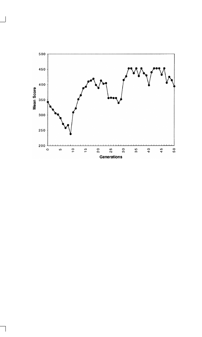
E V O L V I N G N E W S T R A T E G I E S
23
Figure 1-1. Prisoner’s Dilemma in an Evolving Environment
generations the trend starts to reverse. Some players evolve a pattern of
reciprocating what cooperation they find, and these reciprocating players
tend to do well because they can do very well with others who recipro-
cate without being exploited for very long by those who just defect. The
average scores of the population then start to increase as cooperation
based upon reciprocity becomes better and better established. So the
evolving social environment led to a pattern of decreased cooperation
and decreased effectiveness, followed by a complete reversal based upon
an evolved ability to discriminate between those who will reciprocate
cooperation and those who will not. As the reciprocators do well, they
spread in the population, resulting in more and more cooperation and
greater and greater effectiveness.
Conclusions
1. The genetic algorithm is a highly effective method of searching for
effective strategies in a huge space of possibilities. Following Sewall
Wright (1977, 452–54), the problem for evolution can be conceptualized
as a search for relatively high points in a multidimensional field of gene

24
C H A P T E R 1
combinations, where height corresponds to fitness. When the field has
many local optima, the search becomes quite difficult. When the number
of dimensions in the field becomes great, the search is even more difficult.
What the computer simulations demonstrate is that the minimal system
of the genetic algorithm is a highly efficient method for searching such a
complex multidimensional space. The first experiment shows that even
with a seventy-dimensional field of genes, quite effective strategies can be
found within fifty generations. Sometimes the genetic algorithm found
combinations of genes that violate the previously accepted mode of oper-
ation (not being the first to defect) to achieve even greater effectiveness
than had been thought possible.
2. Sexual reproduction does indeed help the search process. This was
demonstrated by the much increased chance of achieving highly effec-
tive populations in the sexual experiment compared to the asexual
experiment.
7
3. Some aspects of evolution are arbitrary. In natural settings, one
might observe that a population has little variability in a specific gene. In
other words one of the alleles for that gene has become fixed throughout
the population. One might be tempted to assume from this that the allele
is more adaptive than any alternative allele. However, this may not be the
case. The simulation of evolution allows an exploration of this possibility
by allowing repetitions of the same conditions to see just how much vari-
ability there is in the outcomes. In fact, the simulations show two reasons
why convergence in a population may actually be arbitrary.
a. Genes that do not have much effect on the fitness of the individ-
ual may become fixed in a population because they “hitchhike” on other
genes that do (Maynard Smith and Haigh 1974). For example, in the
simulations some sequences of three moves may very rarely occur, so
what the corresponding genes dictate in these situations may not matter
very much. However, if the entire population are descendants of just a
few individuals, then these irrelevant genes may be fixed to the values
that their ancestors happened to share. Repeated runs of a simulation
allow one to notice that some genes become fixed in one population
but not another, or that they become fixed in different ways in different
populations.
b. In some cases, some parts of the chromosome are arbitrary in
7
In biology, sexual reproduction comes at the cost of reduced fecundity. Thus, if males
provide little or no aid to offspring, a high (up to two-fold) average extra fitness has to
emerge as a property of sexual reproduction if sex is to be stable. The advantage must
presumably come from recombination but has been hard to identify in biology. A simula-
tion model has demonstrated that the advantage may well lie in the necessity to recombine
defenses to defeat numerous parasites (Hamilton et al. 1990). Unlike biology, in artificial
intelligence applications, the added (computational) cost of sexuality is small.

E V O L V I N G N E W S T R A T E G I E S
25
content, but what is not arbitrary is that they be held constant. By being
fixed, other parts of the chromosome can adapt to them. For example,
the simulations of the individual chromosomes had six genes devoted to
coding for the premises about the three moves that preceded the first
move in the game. When the environment was the eight representatives,
the populations in different runs of the simulation developed different
premises. Within each run, however, the populations were usually very
consistent about the premises: the six premise genes had become fixed.
Moreover, within each population these genes usually became fixed quite
early. It is interesting that different populations evolved quite different
premises. What was important for the evolutionary process was to fix the
premise about which history is assumed at the start, so that the other
parts of the chromosome could adapt on the basis of a given premise.
4. There is a tradeoff between the gains to be made from flexibility
and the gains to be made from commitment and specialization (March
1991). Flexibility might help in the long run, but in an evolutionary sys-
tem, the individuals also have to survive in the short run if they are to
reproduce. This feature of evolution arises at several levels.
a. As the simulations have shown, the premises became fixed quite
early. This meant a commitment to which parts of the chromosome
would be consulted in the first few moves, and this in turn meant giving
up flexibility as more and more of the chromosome evolved on the basis
of what had been fixed. This in turn meant that it would be difficult for a
population to switch to a different premise. Thus, flexibility was given up
so that the advantages of commitment could be reaped.
b. There is also a tradeoff between short- and long-term gains in the
way selection was done in the simulation experiments. In any given gen-
eration there would typically be some individuals that did much better
than the average, and some that did only a little better than the average.
In the short run, the way to maximize the expected performance of the
next generation would be to have virtually all of the offspring come from
the very best individuals in the present generation. But this would imply a
rapid reduction in the genetic variability of the population, and a conse-
quent slowing of the evolutionary process later on. If the moderately
successful were also given a chance to have some offspring, this would
help the long-term prospects of the population at the cost of optimizing
in the short run. Thus, there is an inherent tradeoff between exploitation
and exploration, that is, between exploiting what already works best and
exploring possibilities that might eventually evolve into something even
better (Holland 1975, 160).
5. Evolutionary commitments can be irreversible. For example, in
most of the populations facing the environment of the eight representa-
tives, the individuals evolved strategies that are very similar to tit for

26
C H A P T E R 1
tat. Because tit for tat had done best in the computer tournament
itself, I did not think that it would be possible to do much better with an
evolutionary process. But as noted earlier, in about a quarter of the sim-
ulation runs with sexual reproduction, the population did indeed evolve
substantially better strategies—strategies that were quite different from
tit for tat. These highly effective strategies defected on the very first
move, and often on the second move as well, in order to get information
to determine whether the other player was the type that could be ex-
ploited or not. The more common populations of strategies cooperated
from the beginning and employed reciprocity in a manner akin to tit for
tat. Although these more common strategies might easily mutate to try a
defection at the start of the game, such behavior would be extremely
costly unless the individual already had effective ways of using the infor-
mation that resulted. Moreover, once the population had evolved to be
about as effective as tit for tat, such a mutation would have to be quite
effective in order to survive long enough to be perfected. Thus, once the
population takes a specific route (in this case, toward reciprocity) it can
easily become trapped in a local maxima. Indeed, only the fact that
enough simulation runs were conducted led to the discovery that in this
particular environment reciprocity was only a local maxima, and that
something better was in fact possible. In a field situation, such a discov-
ery might not be possible because there might be essentially just one gene
pool.
Topics Amenable to Simulation
The methodology for the genetic simulation developed in this paper can
be used to explore learning processes in game-theoretic settings. Here is a
list of issues that can be studied with genetic simulations, inspired by
analogs to evolutionary biology:
1. Mutation. The simulation approach developed here suggests that
there is an inherent tradeoff for a gene pool between exploration of possi-
bilities (best done with a high mutation rate) and exploitation of the
possibilities already contained in the current gene pool (best done with a
low mutation rate). This in turn suggests the advantage of having muta-
tion rates adapt to the rate of change in the environment.
8
2. Crossover. In sexual reproduction, crossover serves to give each off-
spring genetic material from both parents. Crossover rates that are too
low would frequently give whole chromosomes of genetic material from
a single parent to an offspring. But crossover rates that are too high
8
I owe this suggestion to Michael D. Cohen.

E V O L V I N G N E W S T R A T E G I E S
27
would frequently split up coadapted sets of alleles that are on the same
chromosome. Perhaps the existence of a multiplicity of chromosomes
(rather than one long chromosome) is more than a mechanical conve-
nience, but is an adaptation to the need for low crossover rates without
the disadvantage of having each offspring being likely to get genetic ma-
terial from only one parent.
3. Inversion. Inversion changes the order of the genes in a chromo-
some. It can bring coadapted sets of alleles closer together on the chro-
mosome so that they will be split apart by crossover less often. How is
the ideal rate of inversion determined?
4. Coding principles. Biological chromosomes are known to contain
material that does not directly code for proteins, but performs other roles
such as marking the boundaries of genes, or perhaps serves no function at
all. Genetic material may also appear in highly redundant form in the
chromosome. Genetic simulation experiments might shed new light on
the theoretical implications of various coding schemes and their possible
role in error reduction and regulation. Or they might show how some
genetic material can exist as “free riders.”
5. Dominant and recessive genes. Mendel’s famous experiments dem-
onstrate that dominant and recessive alleles serve to overcome Darwin’s
concern that blending of parental characteristics would eliminate the
variability of a population. Genetic simulation can be used to explore the
implications of these and other genetic mechanisms for the maintenance
of population variability in the face of selection pressure for local opti-
mality. In particular, it should be possible to explore just which types of
phenotypic features are best coded in terms of dominant and recessive
genes, and which are best coded in other systems of genetic expression.
6. Gradual versus punctuated evolution. Genetic simulation experi-
ments might also shed light on the contemporary debate about whether
evolution proceeds in gradual steps or tends to move in fits and starts.
This type of work might require simulations of tens of thousands of gen-
erations, but runs of such length are feasible.
7. Population viscosity. Obstacles to random mating may exist due to
geographic or other forces tending to favor subdivisions of the popula-
tion. Some computer modeling has already been done for models of this
type (Boorman and Levitt 1980, 78–87; Tanese 1989), revealing clues
about the qualitative features of the spread of a social trait based upon
frequency-dependent selection.
8. Speciation and ecological niches. When distinct ecological niches
exist, a single species tends to differentiate into two or more species to
take advantage of the different opportunities offered by the different
niches. In learning terms, differentiation into two or more species means
that a new strategy is formed from ideas represented in only part of the

28
C H A P T E R 1
total population. Genetic simulation can explore this process by helping
to specify the conditions under which the advantages of specialization
outweigh the disadvantages of narrower mating opportunities and re-
duced ecological flexibility. The fundamental point is that thinking about
genetics as a simulation problem gives a new perspective on the function-
ing of learning processes.
The genetic simulations provided in this essay are highly abstract sys-
tems. The populations are very small, and the number of generations is
few. More significantly, the genetic process have only two operators, mu-
tation and crossover. Compared to biological genetics, this is a highly
simplified system. Nevertheless, the genetic algorithm displayed a re-
markable ability to evolve sophisticated and effective strategies in a com-
plex environment.
References
Axelrod, Robert. 1980a. “Effective Choice in the Prisoner’s Dilemma.” Journal
of Conflict Resolution 24: 3–25.
. 1980b. “More Effective Choice in the Prisoner’s Dilemma.” Journal of
Conflict Resolution 24: 379–403.
. 1984. The Evolution of Cooperation. New York: Basic Books.
Axelrod, Robert, and William D. Hamilton. 1981. “The Evolution of Coopera-
tion.” Science 211: 1390–96.
Binmore, Ken, and Larry Samuelson. 1990. “Evolutionary Stability in Repeated
Games Played by Finite Automata.” Center for Research on Economic and
Social Theory, Working Paper 90-17, Department of Economics, University of
Michigan, Ann Arbor, Mich.
Boorman, Scott A., and Paul R. Levitt. 1980. The Genetics of Altruism. New
York: Academic Press.
Goldberg, D. E. 1983. Computer-Aided Gas Pipeline Operation Using Genetic
Algorithms and Machine Learning. Ph.D. diss., University of Michigan (Civil
Engineering).
. 1989. Genetic Algorithms in Search, Optimization, and Machine Learn-
ing. Reading, Mass.: Addison-Wesley.
Grefenstette, John J., ed. 1985. Proceedings of an International Conference on
Genetic Algorithms and Their Applications. Pittsburgh, Penn.: The Robotics
Institute of Carnegie-Mellon University.
Hamilton, William D. 1980. “Sex Versus Non-Sex Versus Parasite.” Oikos 35:
282–90.
. 1982. “Heritable True Fitness and Bright Birds: A Role for Parasites.”
Science 218: 384–87.
Hamilton, William D., Robert Axelrod, and Reiko Tanese. 1990. “Sexual Repro-
duction as an Adaptation to Resist Parasites.” Proceedings of the National
Academy of Sciences (USA) 87: 3566–73.

E V O L V I N G N E W S T R A T E G I E S
29
Holland, John H. 1975. Adaptation in Natural and Artificial Systems. Ann Ar-
bor: University of Michigan Press.
. 1980. “Adaptive Algorithms for Discovering and Using General Patterns
in Growing Knowledge Bases.” International Journal of Policy Analysis and
Information Systems 4: 245–68.
. 1992. “Genetic Algorithms.” Scientific American 267 ( July): 66–72.
Lomborg, Bjorn. 1991. “An Evolution of Cooperation.” Masters thesis, Institute
of Political Science, University of Aarhus, Denmark.
March, James G. 1991. “Exploration and Exploitation in Organizational Learn-
ing.” Organizational Science 2: 71–87.
Maynard Smith, J., and J. Haigh. 1974. “The Hitch-Hiking Effect of a Favorable
Gene.” Genet. Res., Camb. 23: 23–35.
Megiddo, Nimrod, and Avi Wigderson. 1986. “On Play by Means of Computing
Machines.” IBM Research Division, BJ 4984 (52161), Yorktown Heights, N.Y.
Miller, John. 1989. “The Coevolution of Automata in the Repeated Prisoner’s
Dilemma.” Working Paper, 89–003, Santa Fe Institute, Santa Fe, N.M.
Riolo, Rick L. 1992. “Survival of the Fittest Bits.” Scientific American 267 ( July):
114–16.
Rubinstein, Ariel. 1986. “Finite Automata Play the Repeated Prisoner’s Di-
lemma.” Journal of Economic Theory 39: 83–96.
Tanese, Reiko. 1989. “Distributed Genetic Algorithms for Function Optimiza-
tion.” Ph.D. diss., University of Michigan (Computer Science and Engineering).
Wright, Sewall. 1977. Evolution and the Genetics of Populations. Vol. 4, Experi-
mental Results and Evolutionary Deductions. Chicago: University of Chicago
Press.

2
Coping with Noise
The danger of people or nations misunderstanding each other’s actions
has been a long-term interest of mine. Ever since the Cuban Missile Crisis
in 1962, I have been concerned that errors in perception or implementa-
tion could lead to serious conflict. As a child, I was deeply impressed with
the fairy tale of a little boy who came across two dozing giants. He hit
one of them on the head. This provoked a fight between the giants, and
the little boy was able to use the distraction to get past them.
When I set up the computer tournaments for the Prisoner’s Dilemma, I
allowed for the possibility of random errors in a very simple way. I did
this by informing all the entrants that one of the rules in the tournament
would be a purely random strategy. Afterward, I realized that this form
of randomization did not really deal with the problems of possible mis-
understanding of the choice made by the other player or possible mis-
implementation of one’s own intended choice. This was especially prob-
lematic because tit for tat is, in fact, quite sensitive to either kind of
noise in the system. For example, if two players are using tit for tat and
one of them makes a mistake, the echo of this mistake can go on indefi-
nitely. In addition, if other mistakes are made, the two players eventually
oscillate among all four combinations of choices and are never able to
reestablish a sustained pattern of mutual cooperation (Downs et al.
1986).
In The Evolution of Cooperation, I suggested two ways of dealing with
the echo effect. The first was to make the response to a defection some-
what less than the provocation. The second method was for the player
who defected by accident to realize that the other’s response need not call
for yet another defection (Axelrod, 1984, 186–87). These two ideas have
come to be called generosity and contrition.
In 1988, at the time of Gorbachev’s very friendly overtures toward the
West, I had a wonderful opportunity to see how American and Soviet
defense analysts would play a Prisoner’s Dilemma that included noise. At
a U.S.-Soviet conference on interdependence, I invited two of the partici-
pants to play in front of the audience of social scientists. The Soviet
player was Sergei Blagovolin, a specialist in nuclear strategy at the Insti-
tute of World Economy and International Relations. The American
player was Catherine Kelleher, a professor and former member of the
White House staff specializing in international security affairs. I told

C O P I N G W I T H N O I S E
31
them that each of their choices would have a one-in-six chance of being
misimplemented. Both players would know after the fact whether their
own choice had been misimplemented, but they would never know
whether a particular move by the other side had been the intended choice
or not. The players did not know exactly how long the game would last.
The American started off with a deliberate defection, and defected a
total of six times in nine moves. The Soviet player was more cooperative,
defecting only four times. In the debriefing afterwards, he attributed most
of the American defections to misimplementation. When asked why, the
Soviet player said that he expected that Americans were fairly coopera-
tive and that women in particular would be cooperative. The American,
on the other hand, explained that she expected him to think this way.
Therefore she deliberately defected, correctly expecting that she would be
forgiven due to a very generous Soviet policy.
1
The story illustrates an
important moral: noise calls for forgiveness, but too much forgiveness
invites exploitation (Axelrod and Dion 1988).
I did not do any systematic work on how to cope with noise until I saw
an article with the title “A Strategy of Win-Stay, Lose-Shift That Outper-
forms Tit-for-Tat in the Prisoner’s Dilemma Game” (Nowak and Sig-
mund 1993). The article reported a simulation study that included noise
and found that under the particular conditions of the study,
2
the most
successful strategy is one that repeats its previous choice only when it gets
one of the two highest payoffs, namely, the temptation score for exploit-
ing the other player or the reward for mutual cooperation. Unlike tit
for tat, it defects after the other player suffers an exploitation, and it
cooperates after a mutual defection. My reaction to this study was to feel
a little protective of tit for tat. I was therefore very curious to see how
the new strategy would do in a noisy version of the variegated environ-
ment of my computer tournament.
Fortunately, at this time a postdoctoral fellow, Wu Jianzhong, was avail-
able to help. Dr. Wu is a game theorist from the Institute of Automation in
1
In the game, the Soviet defected on moves 2, 3, 7, and 8. The American defected on
moves 1, 3, 4, 5, 8, and 9. The second move by the Soviet was a misimplementation, and the
sixth and ninth American moves were misimplementations. Using the standard payoffs, this
gave the Soviet player fifteen points and the American twenty-five points. Had they both
been playing tit for tat and been contrite after their own misimplementations, the Soviet
player would have defected only on moves 2 and 7; the American player only on moves 3, 6,
and 9. The score would have been 22 and 27 respectively. Both would have done better with
contrition than either did with their combination of exploitation and excessive forgiveness.
2
These conditions include the range of permitted strategies and manner of calculating
success, as well as the presence of noise. The permitted strategies base their choice only on
the outcome of the previous move. The strategies are defined in terms of the conditional
probabilities to cooperate given the four possible outcomes of the previous move. The
payoffs are calculated from long-term averages without discounting.

32
C H A P T E R 2
Beijing who came to work with me at Michigan. Together we reimple-
mented the sixty-three rules of the second round of the computer tourna-
ment on a Macintosh. When originally run in 1978, the round-robin
tournament pushed the capabilities of a large mainframe computer. In
1994, the equivalent amount of computation was an easy job on a per-
sonal computer. We found that adding either generosity or contrition to
tit for tat is an effective way of coping with noise. The Win-Stay, Lose-
Shift strategy did not perform as well in this variegated environment.
The source code and documentation for this and most of the other
programs used in this volume are available on the Internet.
3
The source
code for this chapter includes all of the original tournament submissions
as well as the new strategies.
After our study was published, new theoretical work by Kraines and
Kraines (1995) placed the Win-Stay, Lose-Shift strategy in a broader con-
text of learning rules. Whereas Win-Stay, Lose-Shift updates its choice
based on only the preceding outcome, the broader class of learning rules
called Pavlov has a parameter for how fast or slowly the rule adjusts its
probabilistic behavior based on recent moves.
4
Kraines and Kraines
point out that the Win-Shift, Lose-Stay strategy dates back at least to the
classic book on the Prisoner’s Dilemma by Rapoport and Chammah
(1965), where it was called Simpleton because of its many shortcomings.
The jury is still out on the question of how robust any of the broader
class of Pavlov learning rules might be.
References
Axelrod, Robert. 1984. The Evolution of Cooperation. New York: Basic Books.
Axelrod, Robert, and Douglas Dion, 1988. “The Further Evolution of Coopera-
tion.” Science 242 (9 Dec.): 1385–90.
Downs, George W., David M. Rocke, and Randolph M. Siverson. 1986. “Arms
Races and Cooperation.” In Cooperation Under Anarchy, ed. Kenneth A. Oye,
Princeton, N.J.: Princeton University Press.
Kraines, David, and Vivian Kraines. 1995. “Evolution of Learning Among Pavlov
Strategies in a Competitive Environment with Noise,” Journal of Conflict Res-
olution 39: 439–66.
Nowak, Martin, and Karl Sigmund. 1993. “A Strategy of Win-Shift, Lose-Stay
That Outperforms Tit-for-Tat in the Prisoner’s Dilemma Game.” Nature 364:
56–58.
Rapoport, Anatol, and Albert W. Chammah. 1965. Prisoner’s Dilemma. Ann
Arbor, Mich.: University of Michigan Press.
3
http:/ /pscs.physics.lsa.umich.edu/Software/ComplexCoop.html
4
In our article, Wu and I use Pavlov as shorthand for Win-Stay, Lose-Shift.

Coping With Noise
HOW TO COPE WITH NOISE IN THE ITERATED
PRISONER’S DILEMMA
J I A N Z H O N G W U A N D R O B E RT A X E L R O D
Reprinted from Jianzhong Wu and Robert Axelrod, “How to Cope with Noise in the Iter-
ated Prisoner’s Dilemma,” Journal of Conflict Resolution 39, no. 1 (Mar. 1995): 183–89.
Reprinted by permission of Sage Publications, Inc.
Abstract:
Noise, in the form of random errors in implementing a choice, is a common
problem in real-world interactions. Recent research has identified three approaches
to coping with noise: adding generosity to a reciprocating strategy; adding con-
trition to a reciprocating strategy; and using an entirely different strategy, Pavlov,
based on switching choice whenever the previous payoff was low. Tournament
studies, ecological simulation, and theoretical analysis demonstrate: (1) A gen-
erous version of tit for tat is a highly effective strategy when the players it
meets have not adapted to noise; (2) If the other players have adapted to noise, a
contrite version of tit for tat is even more effective at quickly restoring mutual
cooperation without the risk of exploitation; (3) Pavlov is not robust.
An important feature of interactions in the real world is that choices can-
not be implemented without error. Because the other player does not nec-
essarily know whether a given action is an error or a deliberate choice, a
single error can lead to significant complications. For example, on Septem-
ber 1, 1983, a South Korean airliner mistakenly flew over the Soviet Union
(Hersh 1989). It was shot down by the Soviets, killing all 269 people
aboard. The Americans and Soviets echoed their anger at each other in a
short but sharp escalation of Cold War tensions (Goldstein 1991, 202).
The effects of error have been treated under the rubric of “noise.” The
best way to cope with noise has become a vital research question in game
theory, especially in the context of the iterated Prisoner’s Dilemma.
1
Clearly, when noise is introduced, some unintended defections will occur.
1
Examples of recent theoretical and simulation studies of the noisy Prisoner’s Dilemma
and related games are Bendor et al. (1991), Bendor (1993), Boyd (1989), Fudenberg and
Maskin (1990), Godfray (1992), Kollock (1993), Lindgren (1991), Nowak and Sigmund
(1992, 1993), and Young and Foster (1991). For a review of earlier work, see Axelrod and
Dion (1988).

34
C H A P T E R 2
This can undercut the effectiveness of simple reciprocating strategies. For
example, Molander (1985) has shown that in the presence of any amount
of noise, two tit for tat (TFT) players will in the long run average the
same payoffs as two interacting random players.
Three different approaches to coping with noise have been proposed.
1. Generosity. Allowing some percentage of the other player’s defec-
tions to go unpunished has been widely advocated as a good way to cope
with noise (Molander 1985; May 1987; Axelrod and Dion 1988; Bendor
et al. 1991; Godfray 1992; Nowak and Sigmund 1992). For example, a
generous version of TFT, called GTFT, cooperates 10 percent of the time
that it would otherwise defect. This prevents a single error from echoing
indefinitely.
2. Contrition. A reciprocating strategy such as TFT can be modified to
avoid responding to the other player’s defection after its own unintended
defection. This allows a quick way to recover from error. It is based upon
the idea that one should not be provoked by the other player’s response
to one’s own unintended defection (Sugden 1986, 110; Boyd 1989). The
strategy called Contrite TFT (CTFT) has three states: “contrite,” “con-
tent,” and “provoked.” It begins in content with cooperation and stays
there unless there is a unilateral defection. If it was the victim while con-
tent, it becomes provoked and defects until a cooperation from the other
player causes it to become content. If it was the defector while content, it
becomes contrite and cooperates. When contrite, it becomes content only
after it has successfully cooperated.
3. Win-Stay, Lose-Shift. A completely different strategy can be used,
one based on the principle that if the most recent payoff was high, the
same choice would be repeated, but otherwise the choice would be
changed. This strategy emerged from a simulated evolutionary process
that included noise, but allowed strategies with memory of only the pre-
ceding move (Nowak and Sigmund 1993). Called Pavlov, it cooperates
unless on the previous move it was a sucker (i.e., it cooperated but the
other defected) or the other player was a sucker.
For completeness, we also analyze a fourth strategy, a generous version
of Pavlov, called GPavlov. This strategy acts like Pavlov, but cooperates
10 percent of the time when it would otherwise defect.
The Tournament with Noise
The basis for our analysis is the environment of the sixty-three rules of the
second round of the computer tournament for the Prisoner’s Dilemma
(Axelrod 1984). These strategies provide a heterogeneous environment
embodying a wide variety of ideas designed for doing well in the Prisoner’s

C O P I N G W I T H N O I S E
35
Dilemma game. The lengths of interactions vary, averaging 151 moves. To
this environment we add 1 percent noise, meaning that for each intended
choice there is a 1 percent chance that the opposite choice will actually be
implemented. Although these rules were designed without regard to noise,
they can still be used to provide a useful setting for evaluating how new
strategies will fare in a heterogeneous noisy environment.
The average score of each new rule when paired with the sixty-three
rules of the tournament environment shows how well or poorly each
does in a noisy environment.
2
The highest score is attained by GTFT,
which actually does better than any of the sixty-three rules submitted.
CTFT also does very well, better than all but five of the sixty-three rules.
Pavlov does poorly, ranking below fifty-five of the sixty-three rules. Add-
ing generosity to Pavlov helps only a little: GPavlov ranks below forty-
eight of the sixty-three rules.
To investigate the effects of different levels of noise, the four new rules
were added to the sixty-three original rules, and the expanded tourna-
ment was run at various levels of noise from 0.1 percent to 10 percent.
Figure 2-1 shows the scores of the four new rules as a function of the
noise level. The results show that at all levels of noise, GTFT and CTFT
do well, whereas Pavlov and GPavlov do not. At the lower levels, GTFT
is a little better than CTFT, but when noise is greater than 1 percent,
CTFT is slightly better.
An Ecological Simulation
A more powerful test is to take into account that over time, rules that are
unsuccessful in the noisy environment are less likely than are relatively
successful rules to be used again. A good way to do this is with an ecolog-
ical analysis (Axelrod 1984, 48ff ). In an ecological analysis, the fraction
of the population represented by a given rule in the next “generation” of
the tournament will be proportional to that rule’s tournament score in
the previous generation. When this process is repeated over many genera-
tions, the proportion of the various rules changes, and the environment
faced by each rule tends to emphasize those rules that have been doing
relatively well in the noisy setting. The ecological simulation shows what
happens when the rules that are ineffective in dealing with noise become
a smaller part of the population and those that are effective at dealing
with noise become a larger proportion of the population.
The process begins with equal proportions of sixty-seven rules: the
sixty-three original rules and the four new ones. The noise level is set at 1
2
To assure stability of these results, the scores are averaged over twenty replications of
the entire tournament.
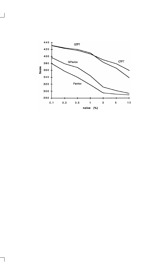
36
C H A P T E R 2
Figure 2-1. Performance as a Function of Noise
percent. The proportion of each rule is updated for 2,000 generations.
Figure 2-2 shows the performance over time of the six rules that did best
at the end of this process. R8, the rule that ranked eighth in the original
tournament, did quite well over the first few hundred generations, but
then slowly declined as the process continued to deemphasize rules that
were doing poorly in the noisy environment. By generation 1,000, CTFT
was the leader. It continued to grow, eventually becoming 97 percent of
the population at generation 2,000. GTFT had some early success, but
then faded. Both versions of Pavlov declined to less than one part in a
million as early as the hundredth generation. The clear winner in this
ecological simulation with noise was CTFT.
Strategic Analysis
Both Pavlov and the contrite version of tit for tat have the desirable
property that when playing with their twin they can quickly recover from
an isolated error. If one of two Pavlov players defects due to an isolated
error, both will defect on the next move, and then both will cooperate on
the following move. If one of two CTFT players defects, the defecting
player will contritely cooperate on the next move and the other player
will defect, and then both will be content to cooperate on the following
move. Unfortunately for a player using Pavlov, its willingness to cooper-
ate after a mutual defection can give the other player an incentive to
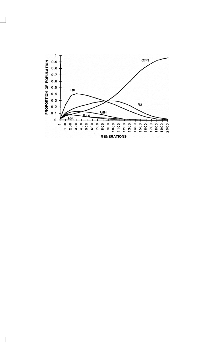
C O P I N G W I T H N O I S E
37
Figure 2-2. Ecological Simulation. Note: The strategies are the sixty-three origi-
nal rules plus GTFT, CTFT, Pavlov and GPavlov. R3 is the rule that ranked third
in original tournament, R4 is the rule that ranked fourth, etc. The results are
shown for the top six rules in the 2,000th generation. The noise level is 1 percent.
simply defect all the time.
3
The tournament and the ecological analysis
both show that although Pavlov may do well with its own twin, its suc-
cess is not robust.
Generosity is effective at stopping the continuing echo of a single error,
whether the error was one’s own or the other player’s. The level of gener-
osity determines how quickly an error can be corrected and cooperation
restored. The problem is that generosity requires a tradeoff between the
speed of error correction and the risk of exploitation (Axelrod and Dion
1988).
Contrition is effective at correcting one’s own error, but not the error
of the other player. For example, if CTFT is playing TFT and the TFT
player defects by accident, the echo will continue until another error oc-
curs. Thus, in the original environment of sixty-three rules that were not
designed to deal with noise, contrition was slightly less effective than
generosity when noise was 1 percent or less. On the other hand, the eco-
logical simulation showed that contrition is very effective as the environ-
ment becomes dominated by rules that are successful in the noisy envi-
ronment. As the population becomes adapted to noise, contrition
3
It pays to always defect when playing with Pavlov at low levels of noise if alternating T
and P is better than always getting R. With standard notation, this is true when T
⫹ wP ⬎
R
⫹ wR or w ⬍ (T ⫺ R)/(R ⫺ P). Thus, with the standard payoffs of T ⫽ 5, R ⫽ 3, P ⫽ 1, S
⫽ 0, and any w ⬍ 1, it pays to always defect when playing with Pavlov.

38
C H A P T E R 2
becomes more and more effective. In a population adapted to noise, cor-
recting one’s own errors is sufficient because the players one meets are
also likely to be good at correcting their own errors.
Conclusion
In the presence of noise, reciprocity still works, provided that it is accom-
panied by either generosity (some chance of cooperating when one would
otherwise defect) or contrition (cooperating after the other player defects
in response to one’s own defection). Pavlov, a strategy based upon chang-
ing one’s own choice after a poor outcome, is not robust.
Generosity can correct an error by either player, but contrition can
only correct one’s own error. Thus, when the population of strategies one
is likely to meet has not adapted to the presence of noise, a strategy like
Generous tit for tat is likely to be effective. On the other hand, if the
strategies of the other players one is likely to meet have already adapted
to noise, then a strategy like Contrite tit for tat is likely to be even
more effective because it can correct its own errors and restore mutual
cooperation almost immediately.
References
Axelrod, R. 1984. The Evolution of Cooperation. New York: Basic Books.
Axelrod, R., and D. Dion. 1988. “The Further Evolution of Cooperation.” Sci-
ence 242: 1385–90.
Bendor, J. 1993. “Uncertainty and the Evolution of Cooperation.” Journal of
Conflict Resolution 37: 709–34.
Bendor, J., R. M. Kramer, and S. Stout. 1991. “When in Doubt: Cooperation in a
Noisy Prisoner’s Dilemma.” Journal of Conflict Resolution 35: 691–719.
Boyd, R. 1989. “Mistakes Allow Evolutionary Stability in the Repeated Pris-
oner’s Dilemma.” Journal of Theoretical Biology 136: 47–56.
Fudenberg, D., and E. Maskin. 1990. “Evolution and Cooperation in Noisy Re-
peated Games.” American Economic Review 80: 274–79.
Godfray, H. C. J. 1992. “The Evolution of Forgiveness.” Nature 355: 206–7.
Goldstein, Joshua. 1991. “Reciprocity in Superpower Relations: An Empirical
Analysis.” International Studies Quarterly 35: 195–209.
Hersh, Seymour M. 1986. “The Target is Destroyed”. New York: Random
House.
Kollock, P. 1993. “An Eye for an Eye Leaves Everyone Blind: Cooperation and
Accounting Systems.” American Sociological Review 58: 768–86.
Lindgren, K. 1991. “Evolutionary Phenomena in Simple Dynamics.” In Artificial
Life II: Proceedings of the Workshop on Artificial Life, ed. C. Langton et al.,
295–312. Redwood City, Calif.: Addison-Wesley.

C O P I N G W I T H N O I S E
39
May, R. M. 1987. “More Evolution of Cooperation.” Nature 327: 15–17.
Milinski, M. 1993. “Cooperation Wins and Stays.” Nature 364: 12–13.
Molander, P. 1985. “The Optimal Level of Generosity in a Selfish, Uncertain
Environment.” Journal of Conflict Resolution 29: 611–18.
Nowak, M., and K. Sigmund. 1992. “Tit for Tat in Heterogeneous Populations.”
Nature 355: 250–53.
. 1993. “A Strategy of Win-Stay, Lose-Shift That Outperforms Tit-for-Tat
in the Prisoner’s Dilemma Game.” Nature 364: 56–58.
Sugden, R. 1986. The Economics of Rights, Co-operation, and Welfare. Oxford:
Basil Blackwell.
Young, H. P., and D. Foster. 1991. “Cooperation in the Short and in the Long
Run.” Games and Economic Behavior 3: 145–156.

3
Promoting Norms
My long-standing interest in norms was piqued by an anecdote that I
included in The Evolution of Cooperation (Axelrod 1984, 84–85). It was
one of the many stories from the trench warfare of World War I in which
the two sides showed restraint based upon reciprocity in what they called
“the live and let live system.” But this particular episode went further
than most. It displayed an emerging ethical component. Here is the story
as related by a British officer recalling his experience while facing a Saxon
unit of the German Army:
I was having tea with A Company when we heard a lot of shouting and went
out to investigate. We found our men and the Germans standing on their re-
spective parapets. Suddenly a salvo arrived but did no damage. Naturally both
sides got down and our men started swearing at the Germans, when all at once
a brave German got onto his parapet and shouted out: “We are very sorry
about that; we hope no one was hurt. It is not our fault. It is that damned
Prussian artillery.” (Rutter 1934, 29)
The Saxon apology goes well beyond a merely instrumental effort to
prevent retaliation. It reflects moral regret for having violated a situa-
tion of trust, and shows concern that someone might have been hurt.
My theory of cooperation based on the two-person iterated Prisoner’s
Dilemma helped explain the restraint based upon the selfish interest of
the soldiers on each side. Yet, I was troubled that the theory did not
account for the moral dimension that was clearly present in this exam-
ple and was probably very important for the development and mainte-
nance of norms.
My interest in norms as a possible aid to international cooperation was
also heightened by my participation in a large research project led by
Kenneth Oye. The project included historical studies of how cooperation
emerges in the context of international anarchy (Oye 1986). In looking
for common findings in the domain of international political economy
and international security, Robert Keohane and I were struck by the im-
portance of norms in explaining when cooperation succeeded and when
it failed. We were also impressed with the role of international institu-
tions in developing shared understandings of what actually counts as ad-
herence to international norms of conduct (Axelrod and Keohane 1986).

P R O M O T I N G N O R M S
41
I also had a long-standing interest in still another approach to norms,
namely, the emergence of norms as solutions to dilemmas of collective
action, such as pollution and overuse of resources held in common. An
obvious way to model such dilemmas was by extending the two-person
Prisoner’s Dilemma to the n-person Prisoner’s Dilemma. This would pro-
vide a good model of problems such as overgrazing of common land or
excess air pollution. In these situations everyone has an incentive to be
selfish. On the other hand, if everyone is selfish, everyone is worse off
than if they had all made the cooperative choice. The problem was that
the policy advice based on reciprocity that works so well in the two-
person Prisoner’s Dilemma simply does not work for the n-person ver-
sion of the game when there is more than a handful of people involved.
This difficulty had been well documented in both theory and practice
(Olson 1965; Hardin 1968; Schelling 1973).
My interpretation of why the n-person Prisoner’s Dilemma cannot be
resolved with simple reciprocity was that there was no way for the coop-
erating players to focus punishment on a defecting player. Given this in-
terpretation, I thought it would be interesting to explore a new n-person
game in which the players had the added option of punishing just those
who do not cooperate. To avoid making the problem trivial, I also sup-
posed that detection of “cheating” was not automatic, and that punish-
ment was costly to the enforcer as well as the target. My hope was that
the analysis of this game would lead to a deeper understanding of how
and when behavioral norms emerge.
In undertaking an analysis of this norms game, I decided not to use
the assumption of rationality that is standard in game theory. The em-
pirical examples of changing norms suggested to me that when people
make choices in complex settings, they are more likely to use a trial-
and-error approach than a fully rational calculation. Fortunately, I had
an effective tool for the study of trial-and-error learning in a stra-
tegic setting. All that I had to do was adapt the genetic algorithm
I used for the two-person Prisoner’s Dilemma to this new game (see
Chapter 1).
The results for the norms game demonstrated that I needed another
mechanism in order for norms to emerge and prove stable. I dubbed this
additional mechanism “metanorms.” A metanorm is based on the will-
ingness to punish not only those who violate norms, but also anyone else
who fails to punish the violators. Although this was a satisfying strategic
result, I also felt a need to consider the full range of mechanisms that
serve to support a norm that is partially established. Among these less
formal mechanisms is the internalization of values that was exhibited in
the trench warfare example. In preparing this essay, I was delighted to see
that the evolutionary approach to norms could address a wide range of

42
C H A P T E R 3
problems, from the demise of slavery and dueling to business reputations
and the proliferation of nuclear weapons.
Although not all of my work has been well received (see the introduc-
tions to Chapters 5 and 7, for example), this essay on norms has been. An
earlier version was selected as the best paper at the 1985 annual meeting
of the American Political Science Association. The published version was
cited along with my earlier work on the Prisoner’s Dilemma when I re-
ceived a five-year MacArthur Prize Fellowship in 1987. And I was asked
to adapt it for a popular audience (Axelrod 1987). I think this work on
norms was well received because it addressed a widely felt need to find a
basis for cooperation in settings that entail many people, rather than just
two.
Since then, I have wondered whether the sudden collapse of commu-
nism in Eastern Europe and the former Soviet Union could be seen in
terms of the evolution of norms. The analysis of these events by Timur
Kuran (1995) suggests that a key factor was a decrease in the expectation
that protest would be quashed. This is an interesting interpretation that is
similar to the earlier work of Mark Granovetter (1978) on tipping pro-
cesses in collective behavior such as rioting. In both theories, individuals
are willing to act if enough others act first. Under certain situations, a
slight change in the willingness of a few people to act first can get the ball
rolling. Perhaps these works will help illuminate why collective behavior
sometimes evolves gradually and sometimes tips suddenly.
When I give talks about the evolution of norms I often stress the
emergence of norms at the global scale, such as the norms against colo-
nialism, racial discrimination, and torture. I have been challenged by
the question of whether different societies are likely to resist the imposi-
tion of norms they consider foreign. For example, won’t societies that
practice female genital mutilation resist Western efforts to eliminate that
practice? My response is a relatively optimistic one. I expect that as the
facts become widely publicized, the practice will become so abhorrent
in the West that pressure will be brought to bear. After all, when Utah
applied to join the Union as a state, the Mormons discovered that po-
lygamy was not necessary. Likewise, when the governments find that
they are risking political and economic ostracism, they may discover
that female genital mutilation need not be tolerated. It may take a de-
cade or two, but I suspect that a global norm against female genital mu-
tilation will take hold.
Although cultural uniformity is certainly not a value in itself, it seems
to me that the spread of global norms has generally been a progressive
process. If colonialism, dueling, and slavery have been virtually elimi-
nated, perhaps other forms of violence and assaults on human dignity
can follow.

P R O M O T I N G N O R M S
43
References
Axelrod, Robert. 1984. The Evolution of Cooperation. New York: Basic Books.
. 1987. “Laws of Life: How Standards of Behavior Evolve.” The Sciences
27 (Mar./Apr.): 44–51.
Axelrod, Robert, and Robert Keohane. 1986. “Achieving Cooperation Under
Anarchy.” In Cooperation Under Anarchy, ed. 226–54. Princeton University
Press.
Granovetter, Mark. 1978. “Threshold Models of Collective Behavior.” American
Journal of Sociology 83: 1420–43.
Hardin, Garrett. 1968. “The Tragedy of the Commons.” Science 162: 1243–48.
Kuran, Timur. 1995. Private Truths, Public Lies. Cambridge, Mass.: Harvard
University Press.
Olson, Mancur, Jr. 1965. The Logic of Collective Action. Cambridge, Mass.: Har-
vard University Press.
Oye, Kenneth, ed. 1986. Cooperation Under Anarchy. Princeton N.J.: Princeton
University Press. The essays in this book originally appeared in the October
1985 issue of World Politics.
Rutter, Owen, ed. 1934. The History of Seventh (Services) Battalion, The Royal
Sussex Regiment 1914–1919. London: Times Publishing Company.
Schelling, Thomas. 1973. “Hockey Helmets, Concealed Weapons, and Daylight
Saving: A Study of Binary Choices with Externalities.” Journal of Conflict Res-
olution 17: 381–428.

Promoting Norms
AN EVOLUTIONARY APPROACH TO NORMS
R O B E RT A X E L R O D
Reprinted by permission from Robert Axelrod, “An Evolutionary Approach to Norms,”
American Political Science Review 80, no. 4 (Dec. 1986): 1095–1111.
Abstract:
Norms provide a powerful mechanism for regulating conflict in groups, even
when there are more than two people and no central authority. This essay
investigates the emergence and stability of behavioral norms in the context of a
game played by people of limited rationality. The dynamics of this new norms
game are analyzed with a computer simulation based upon the evolutionary
principle that strategies shown to be relatively effective will be used more in the
future than less effective strategies. The results show the conditions under
which norms can evolve and prove stable. One interesting possibility is the
employment of metanorms, the willingness to punish someone who did not
enforce a norm. Many historical examples of domestic and international norms
are used to illustrate the wide variety of mechanisms that can support norms,
including metanorms, dominance, internalization, deterrence, social proof,
membership in groups, law, and reputation.
An established norm can have tremendous power. This is illustrated by a
historical instance of the norm of dueling. In 1804 Aaron Burr challenged
Alexander Hamilton to a duel. Hamilton sat down the night before the
duel was to take place and wrote down his thoughts. He gave five reasons
against accepting the duel: his principles were against shedding blood in a
private combat forbidden by law; he had a wife and children; he felt a
sense of obligation toward his creditors; he bore no ill against Colonel
Burr; and he would hazard much and could gain little. Moreover, he was
I owe a great deal to Stephanie Forrest, my research assistant, and to those who helped
me think about norms: Michael Cohen, Jeffrey Coleman, John Ferejohn, Morris Fiorina,
Robert Gilpin, Donald Herzog, John Holland, Melanie Manion, Ann McGuire, Robert
Keohane, Robert McCalla, Amy Saldinger, Lynn Sanders, Kim Scheppele, Andrew Sobel,
Charles Stein, Laura Stoker, and David Yoon. I am also pleased to thank those who helped
support various aspects of this work: the Harry Frank Guggenheim Foundation, the Na-
tional Science Foundation, the Sloan Foundation, and the Michigan Memorial Phoenix
Project.

P R O M O T I N G N O R M S
45
reluctant to set a bad example by accepting a duel. Yet he did accept,
because “the ability to be useful, whether in resisting mischief or effecting
good, in those crises of our public affairs which seem likely to happen,
would probably be inseparable from a conformity with public prejudice
in this particular” (Truman 1884, 345–48). In other words, the prospect
of sanctions imposed by the general public in support of dueling caused
Hamilton to risk, and ultimately to lose, his life—a powerful norm in-
deed, and yet one that has all but disappeared today after centuries of
power over life and death.
Today, norms still govern much of our political and social lives. In
politics, civil rights and civil liberties are as much protected by informal
norms for what is acceptable as they are by the powers of the formal legal
system. Leadership is itself subject to the power of norms, as Nixon
learned when he violated political norms in trying to cover up Watergate.
The operation of Congress is shaped by many norms, including those
governing reciprocity (Matthews 1960) and apprenticeship (Krehbiel
1985). Across many nations, tolerance of opposition is a fragile norm
that has great impact on whether a democracy can survive in a given
country (Almond and Verba 1963; Dahl 1966). In international political
economy, norms are essential for the understanding of the operations of
many functional domains such as banking, oil, and foreign aid (Axelrod
and Keohane 1985; Keohane 1984; Krasner 1983). Even in the domain
of power politics, norms have virtually wiped out colonialism, inhibited
the use of chemical warfare, and retarded the spread of nuclear weapons.
Not only are norms important for many central issues in political sci-
ence, but they are vital to the other social sciences as well. Sociology
seeks to understand how different societies work, and clearly norms are
important in these processes (e.g., Opp 1979; Opp 1983). Anthropology
frequently deals with the unique features of various peoples by describing
in great detail their practices and values, as in the case of feuding (e.g.,
Black-Michaud 1975). Psychologists are concerned with how people in-
fluence each other and the manner in which an individual becomes social-
ized into a community (e.g., Darley and Batson 1973; Sherif 1936). Econ-
omists are becoming interested in the origin and operation of norms as
they have come to realize that markets involve a great deal of behavior
based on standards that no one individual can determine alone (e.g., Fur-
ubotn and Pejovich 1974; Schotter 1981).
Large numbers of individuals and even nations often display a great
degree of coordinated behavior that serves to regulate conflict. When this
coordinated behavior takes place without the intervention of a central
authority to police the behavior, we tend to attribute the coordinated
behavior and the resulting regulation of conflict to the existence of
norms. To make this appeal to norms a useful explanation, we need a

46
C H A P T E R 3
good theory of norms. Such a theory should help explain three things:
how norms arise, how norms are maintained, and how one norm dis-
places another.
One of the most important features of norms is that the standing of a
norm can change in a surprisingly short time. For example, after many
centuries of colonialism, the intolerance of colonial dependence took
hold in the relatively short period of just two decades after World War II.
Before and after such a transition, the state of affairs seems very stable
and perhaps even permanent. For this reason, awareness of a given norm
is most intense precisely when it is being challenged. Examples of norms
being challenged today include the right to smoke in public without ask-
ing permission, the use of gender-laden language, and the prohibition
against the use of chemical warfare. Some of these challenges will succeed
in establishing new norms, and some will fail altogether. Thus, what is
needed is a theory that accounts not only for the norms existing at any
point in time, but also for how norms change over time. To clarify these
processes, one must first be clear about exactly what is being discussed.
In this next section the evolutionary approach to be used in this essay is
explained. Following this, the results of computer simulations of the evo-
lution of norms are presented. The computer simulations are then ex-
tended to include a specific mechanism for the enforcement of norms,
called metanorms. After these formal models are investigated, a wide
variety of processes that might help to sustain norms are discussed, along
with suggestions about how they too can be modeled. The question of the
origin and content of norms is considered, and finally, a summary and
conclusion presents the findings of this paper in the broad context of
social and political change.
The Evolutionary Approach
Norms have been defined in various ways in the different literatures and
even within the same literature. The three most common types of defini-
tions are based upon expectations, values, and behavior. That these dif-
ferent definitions are used for the same concept reflects how expectations,
values, and behavior are often closely linked. Definitions based upon ex-
pectations or values are favored by those who study norms as they exist
in a given social setting. Such definitions are convenient because inter-
views can elicit the beliefs and values of the participants, whereas system-
atically observing their actual behavior is more difficult. Because for
many purposes the most important thing is actual behavior, a behavioral
definition will be used in this study.

P R O M O T I N G N O R M S
47
definition: A norm exists in a given social setting to the extent that individuals
usually act in a certain way and are often punished when seen not to be acting
in this way.
This definition makes the existence of a norm a matter of degree,
rather than an all or nothing proposition, which allows one to speak of
the growth or decay of a norm. According to this definition, the extent to
which a given type of action is a norm depends on just how often the
action is taken and just how often someone is punished for not taking it.
To investigate the growth and decay of norms, I have formulated a
norms game in which players can choose to defect and to punish those
they have seen defecting. The goal of the investigation is to see when
cooperation based upon emerging norms will develop. Ultimately, the
purpose is to learn what conditions favor the development of norms so
that cooperation can be promoted where it might not otherwise exist or
be secure.
To see what rational actors would do in a particular setting, a game-
theory approach can be used. Game theory assumes the players are fully
rational and choose the strategy that gives the highest expected utility
over time, given their expectations about what the other players will do.
Recent work by economists has shown great sophistication in dealing
with problems of defining credible threats and of showing the conse-
quences of requiring actors’ expectations about each other to be consis-
tent with the experience that will be generated by the resulting actions
(Abreu et al. 1985; Friedman 1971; Kreps and Wilson 1982; Selten
1975).
Although deductions about what fully rational actors will do are valu-
able for their own sake, empirical examples of changing norms suggest
that real people are more likely to use trial-and-error behavior than de-
tailed calculations based on accurate beliefs about the future. Therefore, I
have chosen not to study the dynamics of norms using an approach that
depends on the assumption of rationality.
Instead, I use an evolutionary approach. This approach is based on the
principle that what works well for a player is more likely to be used again,
whereas what turns out poorly is more likely to be discarded (Axelrod
1984). As in game theory, the players use their strategies with each other to
achieve a payoff based upon their own choice and the choices of others. In
an evolutionary approach, however, there is no need to assume a rational
calculation to identify the best strategy. Instead, the analysis of what is
chosen at any specific time is based upon an operationalization of the idea
that effective strategies are more likely to be retained than ineffective

48
C H A P T E R 3
strategies. Moreover, the evolutionary approach allows the introduction
of new strategies as occasional random mutations of old strategies.
The evolutionary principle itself can be thought of as the consequence
of any one of three different mechanisms. It could be that the more effec-
tive individuals are more likely to survive and reproduce. This is true in
biological systems and in some economic and political systems. A second
interpretation is that the players learn by trial and error, keeping effective
strategies and altering ones that turn out poorly. A third interpretation,
and the one most congenial to the study of norms, is that the players
observe each other, and those with poor performance tend to imitate the
strategies of those they see doing better. In any case, there is no need to
assume that the individual is rational and understands the full strategic
implications of the situation.
The evolutionary approach is inherently probabilistic and involves
nonlinear effects. For these reasons, it is often impossible to use deductive
mathematics to determine the consequences of a given model. For-
tunately, computer simulation techniques (e.g., Cyert and March 1963)
provide a rigorous alternative to deductive mathematics. Moreover, sim-
ulation can reveal the dynamics of a process, as well as the equilibrium
points. By simulating the choices of each member of a population of
players and by seeing how the players’ strategies change over time, the
unfolding of a given evolutionary process can be analyzed to determine
its overall implications.
The Norms Game
The norms game is described in Figure 3-1. It begins when an individual
(i) has an opportunity to defect, say by cheating on an exam. This oppor-
tunity is accompanied by a known chance of being observed. The chance
of being observed, or seen, is called S. If S is .5, each of the other players
has an even chance of observing a defection if it takes place. If player i
does defect, he or she gets a payoff of T (the temptation for defecting)
equal to 3, and each of the others are hurt (H) slightly, getting a payoff of
H equal to
⫺1. If the player does not defect, no one gets anything.
So far the game is similar to an n-person Prisoner’s Dilemma (see, e.g.,
G. Hardin 1968; R. Hardin 1982; Schelling 1978). The new feature
comes in the next step. If player i does defect, some of the other players
may see the defection, and those who do may choose to punish the defec-
tor. If the defector is punished (P) the payoff is a very painful P
⫽ ⫺9, but
because the act of punishment is typically somewhat costly, the punisher
has to pay an enforcement cost (E) equal to
⫺2. (See Table 3-1.)
The strategy of a player thus has two dimensions. The first dimension

P R O M O T I N G N O R M S
49
Figure 3-1. Norms Game
of player i’s strategy is boldness (B
i
), which determines when the player
will defect. The player will defect whenever the chance of being seen by
someone is less than the player’s boldness, which is to say, whenever S
⬍
B
i
. The second dimension of a player’s strategy is vengefulness (V
i
),
which is the probability that the player will punish someone who is de-
fecting. The greater the player’s vengefulness, the more likely he or she
will be to punish someone who is spotted defecting.
TABLE 3-1
Example of Payoffs in the Norms Game Attained by a Player with Boldness Equal
to 2/7 and Vengefulness Equal to 4/7
Event
Payoff per Event
Number of Events
Payoff
Defection
T
⫽ 3
1
3
Punishment
P
⫽ ⫺9
1
⫺9
Hurt by others
H
⫽ ⫺1
36
⫺36
Enforcement cost
E
⫽ ⫺2
9
⫺18
Score
⫺60

50
C H A P T E R 3
Simulation of the Norms Game
The simulation of the norms game determines how the players’ strategies
evolve over time. The two dimensions of a strategy, boldness and venge-
fulness, are each allowed to take one of eight levels, from 0/7 to 7/7.
Because the representation of eight levels requires three binary bits, the
representation of a player’s strategy requires a total of six bits, three for
boldness and three for vengefulness.
The simulation itself proceeds in five steps, as follows:
(1) The strategies for the initial population of 20 players are chosen at
random from the set of all possible strategies.
(2) The score of each player is determined from the player’s own
choices and the choices of the other players. Each individual gets four
opportunities to defect. For each of these opportunities, the chance of
being seen, S, is drawn from a uniform distribution between 0 and 1. To
see how the scores are attained, let us focus on an arbitrary player in the
initial population of one of the runs, who will be called Lee. Lee has a
boldness level of 2/7 and vengefulness level of 4/7. The total payoff Lee
achieved was the result of four different kinds of events, as shown in
Table 3-1. Lee defected only once because only one of the four oppor-
tunities had a chance of being seen that was less than Lee’s boldness of
2/7. This defection gave a temptation payoff of T
⫽ 3 points. Unfor-
tunately for Lee, one of the other players observed the defection and
chose to punish it, leading to a loss for Lee of P
⫽ ⫺9 points. In addition
the other players defected a total of 36 times, each hurting Lee H
⫽ ⫺1
point. Finally, Lee observed who was responsible for about half of these
defections and chose to punish each of them with a probability deter-
mined by his vengefulness of 4/7. This led to a punishment of 9 of the
defections at an enforcement cost of E
⫽ ⫺2 each, for a further loss of 18
points. The net result of these four types of events was a total score of
⫺60 for Lee.
(3) When the scores of all the players are determined, individuals
whose strategies were relatively successful are selected to have more off-
spring.
1
The method is to give an average individual one offspring and to
give two offspring to an individual who is one standard deviation more
effective than the average. An individual who is one standard deviation
below the population average will not have his or her strategy repro-
duced at all. For convenience, the number of offspring is adjusted to
maintain a constant population of 20. A final step is the introduction of
some mutation so that new strategies can arise and be tested. This is done
1
The procedure used is inspired by the genetic algorithm of computer scientist John
Holland (1975; 1980).

P R O M O T I N G N O R M S
51
Figure 3-2. Norms Game Dynamics
by allowing a 1 percent chance that each bit of an individual’s new strat-
egy will be altered. This mutation rate gives a little more than one muta-
tion per generation in the entire population.
(4) Steps 2 and 3 are repeated for 100 generations to determine how
the population evolves.
(5) Steps 1 to 4 are repeated to give five complete runs of the
simulation.
The results of the five runs are shown in Figure 3-2. The five circles
indicate the average boldness and vengefulness of a population after 100
generations. Three completely different outcomes appear possible. In one
of the runs, there was a moderate level of vengefulness and almost no
boldness, indicating the partial establishment of a norm against defec-
tion. On two other runs there was little boldness and little vengefulness,
and on the remaining two runs, there was a great deal of boldness and
almost no vengefulness—the very opposite of a norm against defection.
What could be happening?

52
C H A P T E R 3
The way the strategies actually evolve over time is revealed by the
change that takes place in a single generation in a population’s average
boldness and vengefulness. To calculate his, the data are used from all
100 generations of all five runs, giving 500 populations. The populations
with similar average boldness and vengefulness are then grouped to-
gether, and their average boldness and vengefulness one generation later
is measured. The results are indicated by the arrows in Figure 3-2.
Now the various outcomes begin to fit into a common pattern. All five
of the runs begin near the middle of the field, with average boldness and
vengefulness levels near one-half. The first thing to happen is a dramatic
fall in the boldness level. The reason for the decline is that when there is
enough vengefulness in the population, it is very costly to be bold. Once
the boldness level falls, the main trend is a lowering of vengefulness. The
reason for this is that to be vengeful and punish an observed defection
requires paying an enforcement cost without any direct return to the indi-
vidual. Finally, once the vengefulness level has fallen nearly to zero, the
players can be bold with impunity. This results in an increase in boldness,
destroying whatever restraint was established in the first stage of the
process—a sad but stable state in this norms game.
This result raises the question of just what it takes to get a norm estab-
lished. Because the problem is that no one has any incentive to punish a
defection, the next section explores one of the mechanisms that provides
an incentive to be vengeful.
Metanorms
A little-lamented norm of once great strength was the practice of lynch-
ing to enforce white rule in the South. A particularly illuminating episode
took place in Texas in 1930 after a black man was arrested for attacking
a white woman. The mob was impatient, so they burned down the court-
house to kill the prisoner within. A witness said, “I heard a man right
behind me remark of the fire, ‘Now ain’t that a shame?’ No sooner had
the words left his mouth than someone knocked him down with a pop
bottle. He was hit in the mouth and had several teeth broken,” (Cantril
1941, 101). This is one way to enforce a norm: punish those who do not
support it. In other words, be vengeful, not only against the violators of
the norm, but also against anyone who refuses to punish the defectors.
This amounts to establishing a norm that one must punish those who do
not punish a defection. This is what I will call a metanorm.
Metanorms are widely used in the systems of denunciation in commu-
nist societies. When the authorities accuse someone of doing something
wrong, others are called upon to denounce the accused. Not to join in
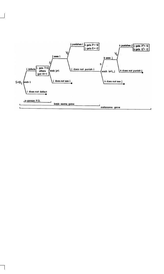
P R O M O T I N G N O R M S
53
Figure 3-3. Metanorms Game
this form of punishment is itself taken as a defection against the group
(Bronfenbrenner 1970; Meyers and Bradbury 1968).
As another example, when the Soviet Union supported the suppression
of the Solidarity movement in Poland, the United States asked its allies to
stop supplying components to the Soviet Union for its new gas pipeline.
The allies, not wanting to pay the enforcement cost of this punishment,
refused. The United States government then undertook the metapunish-
ment of imposing sanctions on foreign companies that defied the sales
ban (New York Times, Jan. 5 and June 19, 1982).
The formulation of a metanorms game can help in the exploration of
the effectiveness of this mechanism. Figure 3-3 shows how the meta-
norms game is based upon an extension of the norms game. If someone
defects, and Lee sees but does not punish that defection, then the other
players have a chance to see and punish Lee. The model makes the critical
assumption that a player’s vengefulness against nonpunishment is the
same as the player’s vengefulness against an original defection.
2
The va-
lidity of this assumption will be addressed later, but first let us see what
effect it has on the evolution of the process.
A set of five runs was conducted with the metanorms game, each done
as before with a population of 20 players and a duration of 100 genera-
2
For convenience, it is also assumed that the chance of being seen not punishing is the
same as the chance of the original defection being seen. The payoff for metapunishment is
P
⬘ ⫽ ⫺9, and the metaenforcement cost is E⬘ ⫽ ⫺2.

54
C H A P T E R 3
Figure 3-4. Metanorms Game Dynamics
tions. The results are shown in Figure 3-4. They are unambiguous. In all
five runs a norm against defection was established. The dynamics are
clear. The amount of vengefulness quickly increased to very high levels,
and this in turn drove down boldness. The logic is also clear. At first there
was a moderate amount of vengefulness in the population. This meant
that a player had a strong incentive to be vengeful, namely, to escape
punishment for not punishing an observed defection. Moreover, when
each of the players is vengeful out of self-protection, it does not pay for
anyone to be bold. Thus the entire system is self-policing, and the norm
becomes well established.
This result is dependent, however, on the population’s starting with a
sufficiently high level of vengefulness. Otherwise the norm still collapses.
Thus, whereas the norms game collapses no matter what the initial con-
ditions are, the metanorms game can prevent defections if the initial con-
ditions are favorable enough.

P R O M O T I N G N O R M S
55
Mechanisms to Support Norms
The simulations of the norms game and the metanorms game have al-
lowed the exploration of some of the important processes in the dy-
namics of norms. The simulation of the norms game shows that relying
on individuals to punish defections may not be enough to maintain a
norm. Therefore, the question to be considered now is, What mecha-
nisms can serve to support a norm that is only partially established? The
evolutionary approach helps to develop a list of such processes, and in
some cases, suggests specific methods for modeling the process by which
a norm can be supported.
Metanorms
As the computer simulations show, the existence of a metanorm can be
an effective way to get a norm started and to protect it once it is estab-
lished. By linking vengefulness against nonpunishers with vengefulness
against defectors, the metanorm provides a mechanism by which the
norm against defection becomes self-policing. The trick, of course, is to
link the two kinds of vengefulness. Without this link, the system could
unravel. An individual might reduce the metavengeance level while still
being vengeful and then later stop being vengeful when others stopped
being metavengeful.
The examples cited earlier suggest that people may well punish those
who do not help to enforce a valued norm. The model suggests norms
can be supported if people tend to have correlated degrees of vengeful-
ness or anger against someone who violates a particular norm and some-
one who tolerates such a violation. What the evolutionary approach has
done is raise the possibility that metanorms are a mechanism that can
help support norms, thus suggesting the interesting empirical question of
whether the two types of vengefulness are indeed correlated. My guess is
that there is such a correlation. The types of defection we are most angry
about are likely to be the ones whose toleration also makes us angry. As
of now, however, the possibility of metanorms remains speculative.
Dominance
Another mechanism for supporting a norm is the dominance of one group
over another. For example, it is no coincidence that in the South, whites
lynched blacks, but blacks did not lynch whites. The whites had two basic
advantages: greater economic and political power, and greater numbers.

56
C H A P T E R 3
Simulation of the effects of power and numbers can be readily done
with slight extensions of the basic model to allow for the existence of two
different groups. The competition between two groups can be modeled
by assuming that the defections of a player only hurt the members of the
other group and are therefore only punished by members of the other
group. Similarly, in the metanorms version of the model, punishments for
not punishing a defector would only occur within a group, as illustrated
by the pop bottle used by one white against another in the lynching ex-
ample discussed above. Moreover, in determining strategies for the next
generation, the strategies of two groups would be allowed to adapt sepa-
rately so that whites learn from whites and blacks learn from blacks.
The two advantages of the whites are modeled separately. Their greater
economic or political power is reflected in their lessened cost of being
punished by a black. This was done by letting P
⫽ ⫺3 for whites while
retaining P
⫽ ⫺9 for blacks. The greater numbers of whites are reflected
directly in the relative size of the two populations, giving the whites a
greater chance to observe and punish a black defection than vice versa.
This was done by letting the population be 20 whites and 10 blacks.
Analysis of runs based upon these conditions shows that resistance to
punishment and increased size can help a group, but only if there are
metanorms. Without metanorms, even members of the stronger group
tend to be free riders, with no private incentive to bear enforcement costs.
This in turn leads to low vengefulness and high boldness in both groups.
When metanorms are added, it becomes relatively easier for the strong
group to keep the weak group from being bold, while it is not so easy for
the weak group to keep the strong one from defecting.
Another form of potential strength is illustrated by the case of a major
power interacting with many smaller nations. For example, the United
States may not only be in a favorable position on a given bilateral interac-
tion but also may have many more bilateral interactions than others.
Thus, its behavior has a greater impact on the development of norms
than would the behavior of a minor power. When Libya wanted to mod-
ify the international norm of the twelve-mile limit of territorial waters to
include the entire Gulf of Sidra, the U.S. fleet deliberately sailed into the
Gulf and shot down two Libyan planes sent up to try to change the norm.
Clearly, the United States was not only stronger but had incentives to
enforce the old norm based upon its naval interests in other parts of the
world.
Although the process of frequent interactions by a single strong player
has not yet been simulated, it is plausible that such a process would help
to establish a norm against defection because the central player would
have a greater unilateral incentive to be vengeful against defections.
Norms can also be promoted by the interests of a few major actors,

P R O M O T I N G N O R M S
57
such as the United States and the Soviet Union’s both working to retard
the proliferation of nuclear weapons. Their actions need not be coordi-
nated in detail as long as together they are important enough to others to
enforce a norm of the major actors’ choice. The logic is somewhat analo-
gous to Olson’s “privileged group” in a collective action problem (Olson
1965, 48–50).
Internalization
Norms frequently become internalized (Scott 1971). This means that vio-
lating an established norm is psychologically painful even if the direct
material benefits are positive. This is frequently observed in laboratory
experiments where subjects are more equitable than they have to be and
explain their behavior by saying things like “you have to live with your-
self.” In terms of the norms game, this type of internalization means that
the temptation to defect, T, is negative rather than positive. If everyone
internalizes a given norm this strongly, there is no incentive to defect and
the norm remains stable. Obviously families and societies work very hard
to internalize a wide variety of norms, especially in the impressionable
young. They do so with greater or lesser success depending on many
factors, including the degree to which the individual identifies with the
group and the degree to which the norm and its sponsors are seen as
legitimate.
3
Clearly, it is rare for everyone in a group to have a norm so strongly
internalized that for each the temptation to defect is actually negative. An
interesting question for future modeling is, How many people have to
internalize a norm in order for it to remain stable?
The logic of the norms game suggests that lowering the temptation to
defect might not be enough. After all, even if most people did not defect,
if no one had an incentive to punish the remaining defectors, the norm
could still collapse. This point suggests that we look for internalization,
not only in the reduced incentive to defect, but also in an increased incen-
tive to punish someone else who does defect.
An increased incentive to punish, through internalization or by some
other means, would lead some people to feel a gain from punishing a
defector. For them, the payoff from enforcement, E, would actually be
positive. Such people are often known as self-righteous busybodies and
often are not very well liked by those who enjoy a defection now and
then. Given enough people who enjoy enforcing the norm, the question
3
Marx goes as far as to say that social norms are merely reflections of the interests of the
ruling class, and the other classes are socialized into accepting these norms under “false
consciousness.”

58
C H A P T E R 3
of its maintenance then becomes whether the chance is high or low that
the defection will be seen.
Deterrence
In the norms game and the metanorms game the players do not look
ahead. Instead they try a particular strategy, see how it does, compare
their payoff with the payoff of others, and switch strategies if they are
doing relatively poorly. Although trial and error is a sensible way of mod-
eling players of very limited rationality, it does not capture the idea that
players may have a great enough understanding of the situation to do
some forward-looking calculations as well as backward-looking compar-
isons with others. In particular, a person may realize that even if punish-
ing a defection is costly now, it might have long-term gains by discourag-
ing other defections later.
A good example is the strong U.S. response to New Zealand’s refusal
in February 1985 to allow a U.S. destroyer into Aukland harbor without
assurances that it did not carry nuclear weapons. The U.S. government
presumably did not care very much about nuclear access to New Zealand
ports, but it did care a great deal about deterring the spread of a new
norm of “nuclear allergy” among its many allies in other parts of the
world (Arkin and Fieldhouse 1985).
Social Proof
An important principle from social psychology is “social proof,” which
applies especially to what people decide is correct behavior. As Cialdini
(1984, 117) explains,
we view a behavior as more correct in a given situation to the degree that we
see others performing it. Whether the question is what to do with an empty
popcorn box in a movie theater, how fast to drive on a certain stretch of high-
way, or how to eat chicken at a dinner party, the actions of those around us will
be important in defining the answer.
The actions of those around us serve several functions. First, they provide
information about the boldness levels of others, and indirectly about the
vengefulness of the population. Hence, we can infer something about
whether it pays for us to be bold or not. Second, the actions of others
might contain clues about what is the best course of action even if there is
no vengefulness. For example, people may be driving slowly on a certain
stretch of highway, not because there is a speed trap there, but because

P R O M O T I N G N O R M S
59
the road is poorly paved just ahead. Either way, the actions of others can
provide information about how the population has been adapting to a
particular environment. If we are new to that environment, this is valu-
able information about what our own behavior should be (Asch 1951;
Asch 1956; Sherif 1936). The actions of others provide information
about what is proper for us, even if we do not know the reasons. Finally,
in many cases, by conforming to the actions of those around us, we fulfill
a psychological need to be part of a group.
Our propensity to act on the principle of social proof is a major mecha-
nism in the support of norms. The current model of norms already has a
form of this mechanism built in: when a relatively unsuccessful individual
seeks a new strategy, that strategy is selected from those being used by the
rest of the population. This is a form of social proof, refined by giving
weight to the more successful strategies being employed in the population.
In cases where other people differ in important ways, the principle of
social proof tends to apply to those who are most like us. This too is easy
to build into simulations with more than one group. In the simulation of
blacks and whites, the blacks look only to other blacks when selecting a
new strategy, and the whites look only to other whites. This makes good
sense because a strategy that is very successful for a white might be disas-
trous if employed by a black.
Membership
Another mechanism for the support of norms is voluntary membership in
a group working together for a common end.
4
Contracts, treaties, alli-
ances, and memberships in social groups all carry with them some power
to impose obligations upon individuals. The power of the membership
works in three ways. First, it directly affects the individual’s utility func-
tion, making a defection less attractive because to defect against a volun-
tarily accepted commitment would tend to lower one’s self-esteem.
Second, group membership allows like-minded people to interact with
each other, and this self-selection tends to make it much easier for the
members to enforce the norm implicit in the agreement to form or join a
group. Finally, the very agreement to form a group helps define what is
expected of the participants, thereby clarifying when a defection occurs
and when a punishment is called for.
One might suppose it would be easy for a bold individual to join and
then exploit a group that had gathered together in the expectation of
mutual compliance. Actually, this does not usually happen, in part be-
4
I thank David Yoon and Lynn Sanders for pointing this out to me.

60
C H A P T E R 3
cause the factors just outlined tend to isolate a defector and make it rela-
tively easy for the others to be vengeful—especially with the help of
metanorms. Another factor is that, according to recent experimental evi-
dence, cooperators are more likely to stay in a group than are defectors
(Orbell et al. 1984). This happens because cooperators have a stronger
ethical or group-regarding impulse than defectors, a factor that led them
to cooperate in the first place.
The metanorms game can be expanded to include the choice of
whether to join a group or not.
5
In general, the value to a person of
joining a group would depend on how many others joined. Each player
would make this choice at the start of the game. Then the interactions
concerning defections and punishments would occur as before, with the
interactions limited to those who had actually joined. As an example, an
alliance for collective security would include a group of nations that had
joined for this common purpose. Once a nation had joined, a defection
would consist of not supporting the alliance in some collective security
task. A defection would hurt the other members of the alliance, and some
of them might choose to punish the defector; they might also choose to
punish someone who did not punish the defector. Typically, the larger the
number of nations joining the group, the greater the benefits of coopera-
tion would be for its members.
In the political sphere, voluntary membership taking the form of a
social contract has been a powerful image for the support of democratic
forms of governance. In effect, a mythical agreement is used to give legit-
imacy to a very real set of laws and institutions.
Law
Norms often precede laws but are then supported, maintained, and ex-
tended by laws. For example, social norms about smoking in public are
now changing. As more and more people turn vengeful against someone
who lights up in a confined space, fewer and fewer smokers are so bold as
to do so without asking permission. As this norm becomes firmer, there is
growing support to formalize it through the promulgation of laws defin-
ing where smoking is and is not permitted.
6
A law supports a norm in several ways. The most obvious is that it
5
I thank David Yoon for formulating this variant of the metanorms game and the appli-
cation to alliances that follows.
6
The same process of formalizing norms applies to private laws and regulations, as in
the case of a business that issues an internal rule about who is responsible for making
coffee.

P R O M O T I N G N O R M S
61
supplements private enforcement mechanisms with the strength of the
state. Because enforcement can be expensive for the individual, this can
be a tremendous asset. In effect, under the law the collective goods prob-
lem of enforcement is avoided because selective incentives are given to
specialized individuals (inspectors, police, judges, etc.) to find and punish
violations.
The law also has a substantial power of its own, quite apart from
whether it is or can be enforced. Many people are likely to take seriously
the idea that a specific act is mandated by the law, whether it is a require-
ment to use seat belts or an income tax on capital gains. However, we all
know this respect for the law has its limits, and we suspect that many
people do not pay all the tax they should. Even when enforcement is
possible and is attempted, the strength of the law is limited. In most
cases, the law can only work as a supplement (and not a replacement)
for informal enforcement of the norm. The failure of Prohibition is a
classic example of an attempt to enforce a norm without sufficient social
support.
In addition to enforcement and respect, a third advantage of the law is
clarity. The law tends to define obligations much more clearly than does
an informal norm. A social norm might say that a landlord should pro-
vide safe housing for tenants, but a housing code is more likely to define
safety in terms of fire escapes. Over the domain covered by the law, the
norm might become quite clear. However, this clarity is gained at the
expense of suggesting that conformity with the law is the limit of one’s
social obligations.
Modeling the power and operation of the law is beyond the scope of
this project. However, it should still be emphasized that often law is the
formalization of what has already attained strength as a social or politi-
cal norm. An important example is civil liberties, the very foundation of a
democratic system. There are laws and constitutional provisions in sup-
port of civil liberties such as freedom of speech, but the legal system can
only protect free speech if there is substantial support for it among a
population willing to tolerate dissent and willing to protect those who
exercise it.
In short, social norms and laws are often mutually supporting. This is
true because social norms can become formalized into laws and because
laws provide external validation of norms. They are also mutually sup-
porting because they have complementary strengths and weaknesses. So-
cial norms are often best at preventing numerous small defections where
the cost of enforcement is low. Laws, on the other hand, often function
best to prevent rare but large defections because substantial resources are
available for enforcement.

62
C H A P T E R 3
Reputation
An important, and often dominant, reason to respect a norm is that vio-
lating it would provide a signal about the type of person you are. For
example, if there is a norm dictating that people should dress formally for
dinner, and you do not, then others might make some quite general infer-
ences about you.
The importance of dressing formally when the occasion requires is not
just that others will punish you for violating the norm (say, by giving you a
disapproving look) but also that they will infer things about you and then
act in ways you wish they would not. This is an example of the signaling
principle: a violation of a norm is not only a bit of behavior having a payoff
for the defector and for others; it is also a signal that contains information
about the future behavior of the defector in a wide variety of situations.
7
There are several important implications of the signaling principle for
the origin and durability of a norm. A norm is likely to originate in a type
of behavior that signals things about individuals that will lead others to
reward them. For example, if a certain accent signals good breeding, then
others may give better treatment to those who speak that way. Once this
happens, more people are likely to try to speak that way. Eventually,
people might be punished (e.g., despised) for not having the right accent.
Thus, what starts out as a signal about one person’s background can
become a norm for all.
8
The signaling principle helps explain how an “is” becomes an
“ought.” As more and more people use the signal to gain information
about others, more and more people will adopt the behavior that leads to
being treated well. Gradually the signal will change from indicating a
rare person to indicating a common person. On the other hand, the ab-
sence of the signal, which originally carried little information, will come
to carry substantial information when the signal becomes common.
When almost everyone behaves in conformity with a signal, those who
do not stand out. These people can now be regarded as violators of a
norm—and dealt with accordingly.
Note that there is an important distinction between a convention,
which has no direct payoffs one way or the other (such as wearing a tie
for men), and a cooperative act, the violation of which leads to injury to
others (e.g., queuing for service). A type of behavior with no direct pay-
offs can become a norm once it develops some signaling value, as is the
7
For the theory of signaling, see Spence (1974). For a theory of how customs can be
sustained by reputations, see Akerlof (1980).
8
Signals can also help to differentiate groups and thereby maintain group boundaries
and cohesiveness.

P R O M O T I N G N O R M S
63
case when fashion leaders adopt a new style (Veblen 1899). Once this
happens, a violator of this style will be looked down upon. Thus the style
will become a norm; individuals will usually follow the style, and those
who do not will likely be punished.
The Origin and Content of Norms
Eight mechanisms have now been identified that can serve to support a
norm that is already at least partially established. What, however, are the
characteristics of the behaviors that arise and then become more and
more established as norms? Or to put it another way, just what is the
content of behavior that might later turn into a norm?
The answer depends on what types of behavior can appear and spread
in a population even when only a few people initially exhibit the behav-
ior. This, in turn, depends on what kind of behavior is likely to be re-
warded and punished for its own sake, independent of whether or not it
is common behavior.
Two of the supporting mechanisms already considered can serve in this
initial role: dominance and reputation. Dominance can work because if
only a few very powerful actors want to promote a certain pattern of
behavior, their punishments alone can often be sufficient to establish it,
even if the others are not vengeful against defections. The implications
for the substance of norms are obvious: it is easier to get a norm started if
it serves the interests of the powerful few.
In fact, many norms obeyed and even enforced by almost everyone
actually serve the powerful. This can happen in forms disguised as equal-
itarian or in forms that are blatantly hierarchical. An apparently equal-
itarian norm is that the rich and the poor are equally prohibited from
sleeping under bridges at night. A blatantly hierarchical norm is that sol-
diers shall obey their officers. Both forms are “norms of partiality,” to use
the term of Ullmann-Margalit (1977).
To say that the powerful can start a norm suggests a great deal about
the potential substance of such norms. Once started, the strong support
the norms because the norms support the strong.
Dominance is not the only mechanism capable of starting a norm. Rep-
utation can do so as well. Consider, for example, the idea of keeping
one’s promise. In a hypothetical society in which few people kept their
promises, you would be happy to deal with someone who did. You would
find it in your narrow self-interest to continue dealing with such a person,
and this in turn would be rewarding to the promise-keeper. Conversely,
you would try to avoid deals with those you knew did not keep their
promises. You would, in effect, be vengeful against defectors without

64
C H A P T E R 3
having to pay an enforcement cost. Indeed, your enforcement would sim-
ply be the result of your acting in your own interests, based upon the
reputations of others and your calculation about what was good for
yourself.
International regimes depend on just such reputational mechanisms to
get norms started (Keohane 1984). In such cases, counties can be very
deliberate about what promises they make and which ones they want to
keep when the stakes are high (Axelrod 1979). Reputational effects can
also be based upon the limited rationality of trial-and-error learning. If a
person associates another’s response to a particular act (say a refusal to
continue dealing as a reaction to the breaking of a promise), then the
violator can learn not to break promises.
This learning approach suggests the importance of being able to link
the behavior with the response. Behaviors will be easier to establish as
norms if the optimal response of others is prompt and rewarding. Failing
a prompt response, learning can also take place if the delayed punish-
ment is explicitly cited as a response to the earlier defection.
Summary and Conclusion
To study the development of norms, the strategic situation has been mod-
eled as an n-person game. In the basic norms game, everyone has two
types of choice: the choice to cooperate or defect, which affects everyone,
and the choice of whether or not to punish a specific person seen defect-
ing. A player’s strategy is described in terms of how these choices will be
made. A strategy consists of two parameters: boldness (the largest chance
of being seen that will lead to a choice of defection) and vengefulness (the
probability of punishing someone observed defecting). To the extent that
players are vengeful but not very bold, a norm can be said to have been
established.
To study the dynamics of the process, an evolutionary approach was
employed. In this approach, the initial strategies are chosen at random,
and the population of players is given opportunities to defect and to pun-
ish the defections they observe. The evolutionary approach dictates that
strategies proving relatively effective are more likely to be employed in
the future while less effective strategies are dropped. Moreover, strategies
undergo some random mutation so that new ones are always being intro-
duced into the population.
The computer simulation of this process revealed an interesting dy-
namic in the norms game. At first, boldness levels fell dramatically due to
the vengefulness in the population. Then, gradually, the amount of venge-
fulness also fell because there was no direct incentive to pay the enforce-

P R O M O T I N G N O R M S
65
ment cost of punishing a defection. Once vengeance became rare, the
average level of boldness rose again, and the norm completely collapsed.
Moreover, the collapse was a stable outcome.
This result led to a search for mechanisms that could sustain a partially
established norm. One possibility is the metanorm: the treatment of non-
punishment as if it were another form of defection; that is, a player will
be vengeful against someone who observed a defection but did not pun-
ish it. Simulation of the evolution of strategies in this metanorms game
demonstrated that players had a strong incentive to increase their venge-
fulness lest they be punished by others, and this in turn led to a decline of
boldness. Thus, metanorms can promote and sustain cooperation in a
population.
Other mechanisms for the support of norms are also important. These
include dominance, internalization, deterrence, social proof, member-
ship, law, and reputation. In some cases, the resulting norms are hier-
archical rather than equalitarian, and the cooperation exhibited is co-
erced rather than freely offered. A good example is the norm of black
deference in the old South.
Dominance processes have been simulated by subdividing the popula-
tion and letting one segment be relatively resistant to the effects of pun-
ishment by members of the other segment. Internalization can be investi-
gated by studying the effects of making defection costly rather than
rewarding for some of the defectors and by making punishment a plea-
sure rather than a cost for some of the observers of a defection. A more
drastic change in the modeling procedures would be necessary to study
some of the other mechanisms in question.
Norms are important in society and, not surprisingly, have been given
a great deal of attention in the social sciences, including sociology, an-
thropology, political science, psychology, and economics. Although de-
scriptions of actual norms abound, investigations of the reasons for
people to obey or violate a given norm have been much less common.
Even among the strategic approaches to norms, relatively little attention
has been devoted to understanding the dynamics of norms: how they can
get started, how a partial norm can be sustained and become well estab-
lished, and how one norm can displace another. An evolutionary ap-
proach is helpful in studying these dynamics because it can help show
how strategies change over time as a function of their relative success in
an ever-changing environment of other players who are also changing
their own strategies with experience.
A major goal of investigating how cooperative norms in societal set-
tings have been established is a better understanding of how to promote
cooperative norms in international settings. This is not as utopian as it
might seem because international norms against slavery and colonialism

66
C H A P T E R 3
are already strong, while international norms are partly effective against
racial discrimination, chemical warfare, and the proliferation of nuclear
weapons. Because norms sometimes become established surprisingly
quickly, there may be some useful cooperative norms that could be hur-
ried along with relatively modest interventions.
References
Abreu, Dilip, David Pearce, and Ennio Stacchetti. 1985. Optimal Cartel Equi-
libria with Imperfect Monitoring. Minneapolis: University of Minnesota Insti-
tute for Mathematics and Its Applications.
Akerlof, George A. 1980. “A Theory of Social Custom, of Which Unemployment
May Be One Consequence.” Quarterly Journal of Economics 94: 749–75.
Almond, Gabriel, and Sidney Verba. 1963. The Civic Culture. Princeton, N.J.:
Princeton University Press.
Arkin, William, and Richard W. Fieldhouse. 1985. “Focus on the Nuclear Infra-
structure.” Bulletin of the Atomic Scientists 41: 11–15.
Asch, Solomon E. 1951. “Effects of Group Pressure upon the Modification and
Distortion of Judgment.” In Groups, Leadership and Men, ed. Harold
Guetzkow, 177–90. Pittsburgh: Carnegie Press.
. 1956. “Studies of Independence and Conformity: I. A Minority of One
Against a Unanimous Majority.” Psychological Monographs 41: 258–90.
Axelrod, Robert. 1979. “The Rational Timing of Surprise.” World Politics 31:
228–46.
. 1984. The Evolution of Cooperation. New York: Basic Books.
Axelrod, Robert, and Robert O. Keohane. 1985. “Achieving Cooperation Under
Anarchy: Strategies and Institutions.” World Politics 38: 226–54.
Black-Michaud, Jacob. 1975. Cohesive Force: Feud in the Mediterranean and the
Middle East. Oxford: Basil Blackwell.
Bronfenbrenner, Urie. 1970. Two Worlds of Childhood: U.S. and U.S.S.R. New
York: Russell Sage.
Cantril, Hadley. 1941. The Psychology of Social Movements. New York: Wiley.
Cialdini, Robert H. 1984. Influence—How and Why People Agree to Things.
New York: Morrow.
Cyert, Richard M., and James G. March. 1963. A Behavioral Theory of the Firm.
Englewood Cliffs, N.J.: Prentice-Hall.
Dahl, Robert A., ed. 1966. Political Oppositions in Western Democracies. New
Haven: Yale University Press.
Darley, John M., and C. Daniel Batson. 1973. “ ‘From Jerusalem to Jerico’: A
Study of Situational and Dispositional Variables in Helping Behavior.” Journal
of Personality and Social Psychology 27: 100–108.
Friedman, James W. 1971. “A Non-Cooperative Equilibrium for Supergames.”
Review of Economic Studies 38: 1–12.
Furubotn, Eirik G., and Svetozar Pejovich, eds. 1974. The Economics of Property
Rights. Cambridge, Mass.: Ballinger.

P R O M O T I N G N O R M S
67
Hardin, Garrett. 1968. “The Tragedy of the Commons.” Science 162: 1243–48.
Hardin, Russell. 1982. Collective Action. Baltimore: Johns Hopkins University
Press.
Holland, John H. 1975. Adaptation in Natural and Artificial Systems. Ann Ar-
bor: University of Michigan Press.
. 1980. “Adaptive Algorithms for Discovering and Using General Patterns
in Growing Knowledge Bases.” International Journal of Policy Analysis and
Information Systems 4: 245–68.
Keohane, Robert O. 1984. After Hegemony: Cooperation and Discord in the
World Political Economy. Princeton, N.J.: Princeton University Press.
Krasner, Stephen D., ed. 1983. International Regimes. Ithaca, N.Y.: Cornell Uni-
versity Press.
Krehbiel, Keith. 1985. Unanimous Consent Agreements: Going Along in the Sen-
ate.” Working paper no. 568. California Institute of Technology, Social Science
Department.
Kreps, David M., and Robert Wilson. 1982. “Sequential Equilibria.” Economet-
rica 50: 863–94.
Matthews, Donald R. 1960. U.S. Senators and Their World. Chapel Hill: Univer-
sity of North Carolina Press.
Meyers, Samuel M., and William C. Bradbury. 1968. “The Political Behavior of
Korean and Chinese Prisoners of War in the Korean Conflict: A Historical
Analysis.” In Mass Behavior in Battle and Captivity, The Communist Soldier in
the Korean War, ed. Samuel M. Meyers and Albert D. Briderman, 209–338.
Chicago: University of Chicago Press.
Olson, Mancur. 1965. The Logic of Collective Action. Cambridge, Mass.: Har-
vard University Press.
Opp, Karl-Dieter. 1979. “Emergence and Effects of Social Norms—
Confrontation of Some Hypotheses of Sociology and Economics.” Kylos 32:
775–801.
. 1983. “Evolutionary Emergence of Norms.” British Journal of Social
Psychology 21: 139–49.
Orbell, John M., Peregrine Schwartz-Shea, and Randall T. Simmons. 1984. “Do
Cooperators Exit More Readily than Defectors?” American Political Science
Review 78: 163–78.
Schelling, Thomas. 1978. Micromotives and Macrobehavior. New York: W. W.
Norton.
Schotter, Andrew. 1981. Economic Theory of Social Institutions. Cambridge,
Eng.: Cambridge University Press.
Scott, John F. 1971. Internalization of Norms. Englewood Cliffs, N.J.: Prentice-
Hall.
Selten, R. 1975. “Reexamination of the Perfectness Concept for Equilibrium
Points in Extensive Games.” International Journal of Game Theory 4: 25–
55.
Sherif, Muzafer. 1936. The Psychology of Social Norms. New York: Harper and
Brothers.
Spence, A. Michael. 1974. Market Signalling. Cambridge, Mass.: Harvard Uni-
versity Press.

68
C H A P T E R 3
Truman, Ben C. 1884. Field of Honor: A Complete and Comprehensive History
of Dueling in All Countries. New York: Fords, Howard and Hilbert.
Ullmann-Margalit, Edna. 1977. The Emergence of Norms. Oxford: Oxford Uni-
versity Press.
Veblen, Thorstein. 1899. The Theory of the Leisure Class. New York:
Macmillan.

4
Choosing Sides
My interest in how political actors choose sides goes back at least to my
days in graduate school in the 1960’s. For example, my Ph.D. dissertation
on conflict of interest included a chapter on coalition formation in parlia-
mentary democracies. The basic idea was that political parties of differing
ideologies might have to work together to attain a governing majority, but
they seek a set of partners that will cause as little political strain as possible.
In other words, politics minimizes the strangeness of bedfellows. This idea
was contrary to the prevailing view that coalition formation is based solely
upon the number of seats each party holds without regard to their politics
(Riker 1962). My theory worked fairly well in predicting the membership
and duration of Italian coalitions (Axelrod 1970).
The Italian case was relatively easy to analyze because there was a
single left-right ideological dimension along which the parties were ar-
rayed. Therefore I was able to predict that the actual coalitions would
consist of a connected series of parties in this space, and would be no
wider than necessary to form a majority in the parliament. Although the
details vary, the importance of ideological affinity for coalition formation
has since been confirmed across a wide range of parliamentary democra-
cies (e.g., Lijphart 1981; Laver and Shepsle 1996).
In 1986, I first visited the Santa Fe Institute, a center of research on
complexity theory. At the time, there was a great deal of talk about “spin
glasses.” The spin-glass model is derived from a problem in condensed
matter physics. The idea is that each atom tries to align its spin to be
consistent with certain of its neighbors and opposite to the others (Ander-
son 1989; Waldrop 1992, 138–39). This reminded me of my earlier
theme that political parties try to minimize the strangeness of their bed-
fellows. It gave me the idea that the mathematical model of how atoms
“choose” magnetic alignments (or spins) might be helpful for thinking
about how political actors choose sides. In both cases, many independent
actors try to reach an alignment that minimizes their frustration in terms
of the actions taken by all other actors.
1
Everything depends on every-
thing else, but a few collective outcomes are more stable than the others.
1
In retrospect, I see that my study of decision-making styles also employed the idea of
minimization of strain between many elements of an interacting system. In the case of
decision making, the elements were causal arguments connecting policy-relevant variables. I

70
C H A P T E R 4
The spin-glass model was also interesting to me because under certain
circumstances it had a geometric representation in terms of energy land-
scapes. Energy landscapes were very similar to the fitness landscapes that
I was used to from evolutionary biology. The geometric representation of
landscapes was valuable because movement in such an abstract land-
scape suggested a way to simulate an agent-based model of how agents
choose sides.
I realized that if I could measure the affinity of each political actor to
align with each of the others, I could get predictions about what align-
ments would actually form. I chose the case of European nations in-
volved in World War II because there were enough independent actors to
give the theory a good test. Scott Bennett, then a graduate student, and I
developed a way to measure the affinity of each pair of nations in terms
of characteristics that they might share. We also took account of the
relative power of the nations involved. We then did what amounted to an
agent-based simulation in which each of the actors kept trying to change
sides if it had more affinity with the other protocoalition. Our prediction
was simply that the alignment would be one of the few that was stable in
the simulation. The prediction actually worked well. Even better, as we
used data about propensities and power closer and closer in time to the
outbreak of the war, the prediction turned out to be better and better. It
even accounted for the contemporaneous pattern of realignment activ-
ities when the Warsaw Pact disintegrated.
As discussed in the introductory chapter, the main purpose of agent-
based models is not prediction but a deeper understanding of how funda-
mental social processes operate. In this case, however, Scott and I were
also able to operationalize the model and use it to make specific predic-
tions that could be tested with historical data.
This paper has an interesting sequel in which the same theory is em-
ployed in a completely different setting, business coalitions. That story is
Chapter 5.
References
Anderson, Philip W. 1989. “Spin Glass V: Real Power Brought to Bear.” Physics
Today ( July): 9–10.
Axelrod, Robert. 1970. Conflict of Interest. Chicago, Ill.: Markham.
found that there was a strong tendency for an elite policy maker to present arguments that
had no tradeoffs. This eliminated the inconsistencies among different causal paths (Axelrod
1976 and 1977).

C H O O S I N G S I D E S
71
. 1977. “Argumentation in Foreign Policy Settings: Britain in 1918, Mu-
nich in 1938 and Japan in 1970.” Journal of Conflict Resolution 21: 727–56.
, ed. 1976. The Structure of Decision. Princeton, N.J.: Princeton Univer-
sity Press.
Laver, Michael, and Kenneth Shepsle. 1996. Making and Breaking Governments.
New York: Cambridge University Press.
Lijphart, Arend. 1981. “Power-Sharing Versus Majority Rule: Patterns of Cabi-
net Formation in Twenty Democracies.” Government and Opposition 16:
395–413.
Riker, William H. 1962. The Theory of Political Coalitions. New Haven: Yale
University Press.
Waldrop, M. Mitchell. 1992. Complexity: The Emerging Science at the Edge of
Order and Chaos. New York: Simon and Schuster.

Choosing Sides
A LANDSCAPE THEORY OF AGGREGATION
R O B E RT A X E L R O D A N D D . S C O T T B E N N E T T
Adapted from Robert Axelrod and D. Scott Bennett “A Landscape Theory of Aggregation,”
British Journal of Political Science 23 (Apr. 1993): 211–33. Reprinted by permission.
Abstract:
Aggregation means the organization of elements of a system into patterns
that tend to put highly compatible elements together and less compatible ele-
ments apart. Landscape theory predicts how aggregation will lead to align-
ments among actors (such as nations), whose leaders are myopic in their assess-
ments and incremental in their actions. The predicted configurations are based
upon the attempts of actors to minimize their frustration based upon their
pairwise propensities to align with some actors and oppose others. These at-
tempts lead to a local minimum in the energy landscape of the entire system.
The theory is supported by the results of the alignment of seventeen European
nations in the Second World War. The theory has potential for application to
coalitions of business firms, political parties in parliaments, social networks,
social cleavages in democracies, and organizational structures.
This article presents a formal theory of aggregation, called landscape
theory, and provides two tests of the theory. “Aggregation” means the
organization of elements of a system in patterns that tend to put highly
compatible elements together and less compatible elements apart. Land-
scape theory uses abstract concepts from the physical sciences and biol-
ogy that have proved useful in studying the dynamics of complex sys-
tems. These concepts provide a way of thinking about the many
possible ways in which elements of a system can fit together, predicting
which configurations are most likely to occur, how much dissatisfaction
with the outcome is inevitable and how the system will respond to
changes in the relationship between the elements. As applied to politi-
cal, economic, and social problems, landscape theory can be used to
For helpful suggestions the authors thank Erhard Bruderer, Michael Cohen, John Hol-
land, Will Mitchell, David Sanders, Carl Simon, Robert Thomas, and anonymous re-
viewers. This work was supported by National Science Foundation grants SES 8808459
and SES 9106371.

C H O O S I N G S I D E S
73
analyze a wide variety of aggregation problems that have previously
been considered in isolation:
1. international alignments,
2. alliances of business firms to set standards,
3. coalitions of political parties in parliaments,
4. social networks,
5. social cleavages in democracies, and
6. organizational structures.
In order to be useful, a theory of aggregation should have the following
properties:
a. The theory should provide a coherent explanation of why some particu-
lar aggregations (alliances, coalitions, organizational structures, etc.) form in a
given system, and not others.
b. The theory should illuminate the dynamics of aggregation to provide a
deeper understanding of the actual process involved as well as the end result.
c. The theory should be general enough to apply to many domains of poli-
tics and society.
d. The theory should be simple enough to illuminate some fundamental
aspects of aggregation.
e. The theory should be capable of being operationalized so that its predic-
tions can be tested.
This essay seeks to demonstrate that the landscape theory of aggrega-
tion offers excellent promise of fulfilling all five of these conditions. In
particular, this article provides the first empirical test of a theory of align-
ment in international politics. It does so by providing a new theoretical
approach to aggregation dynamics and by being practical about measure-
ment. The significance of landscape theory is that it can provide a deeper
understanding of a wide variety of important aggregation processes in
politics, economics and society. How the elements of a system fit together
has important implications for such vital issues as the balance of power
in international politics, the way in which competing businesses can
agree to set standards for their products, the construction of ruling coali-
tions among parties in parliamentary democracies and the ways political
parties appeal to voters in a society with overlapping and cross-cutting
cleavages.
By using a common set of concepts to explain a variety of distinct
subjects, the current understanding of each subject can be used to help
illuminate the others. Moreover, by using a common theory, such as land-
scape theory, one might reach a deeper understanding of how the aggre-
gation process in each of these domains is similar to the others and how
each is different from the others. In addition to purely scientific signifi-

74
C H A P T E R 4
cance, landscape theory can be used as a guide to policy. For example, by
providing a coherent explanation of which international alignments are
likely to form, it can suggest where leverage can most efficiently be ap-
plied to move from one configuration to another. As another example,
the theory could suggest which domestic political coalitions are inher-
ently unstable and which would become stable if critical subgroups could
be induced to make minor changes.
The next section formally presents landscape theory, followed by a
section on how the concept of an abstract landscape has been used in the
physical and natural sciences. Then the operationalization and test of the
theory are provided for a case from international politics. The penulti-
mate section shows how the theory could be applied to five other do-
mains as well. The final section considers how the foundations of land-
scape theory can be made more rigorous.
Landscape Theory
This section explains the formal aspects of the theory, shows how the
concepts of the approach may help to illuminate an aggregation process
and enumerates the predictions that can be derived from the theory.
Landscape theory predicts how actors will form alignments. To help
keep the terminology as simple as possible, the language of international
alignments will be used. The theory makes two basic assumptions, both
drawn from the recognition that it is difficult for a national leadership to
assess the value of each potential alignment. The first assumption is that a
nation is myopic in its assessments. In other words, a national leadership
evaluates how well it gets along with any other nation independent of all
the other members in the system. By making only pairwise evaluations,
the national leadership avoids the difficult problem of assessing all com-
binations of nations at once.
The second basic assumption of landscape theory is that adjustments
to alignments take place by incremental movement of individual nations.
This rules out the possibility that a coalition will form within an align-
ment and then switch allegiance as a block. This strong assumption is
appropriate when information regarding payoffs is uncertain, resulting in
causal ambiguity between alignment actions and payoffs, and a conse-
quent increase in negotiation costs and a reduction in the ability of na-
tions to use side payments to arrive at an optimal solution.
Landscape theory begins with a set of n actors (for example, nations).
The size of a nation, s
i
⬎ 0, is a reflection of the importance of that
country to others. Size might be measured by demographic, industrial, or

C H O O S I N G S I D E S
75
military factors, or a combination of these, depending on what is taken to
be important in a particular application.
The key premise of landscape theory is that each pair of nations, i and
j, has a propensity, p
ij
, to work together. The propensity number is posi-
tive and large if the two nations get along well together and negative if
they have many sources of potential conflict. Put another way, propensity
is a measure of how willing the two nations are to be in the same coali-
tion together. If one country has a source of conflict with another (such as
a border dispute), then the second country typically has the same source
of conflict with the first. Thus the theory assumes that propensity is sym-
metric, so that p
ij
⫽ p
ji
.
A configuration is a partition of the nations, that is, a placement of
each nation into one and only one grouping. An example is the postwar
situation in which the nonneutral nations of Europe were divided be-
tween NATO and the Warsaw Pact. A specific configuration, X, deter-
mines the distance, d
ij
, between any two countries, i and j. In the simplest
version of the theory all countries are assumed to be in one of two pos-
sible groupings, so we can let distance be 0 if the two countries are in the
same grouping, and 1 if the two countries are in different groupings. In
other situations, other measures of distance in a configuration will be
appropriate.
1
Using distance and propensity, it is now possible to define a measure of
frustration: how poorly or well a given configuration satisfies the propen-
sities of a given country to be near or far from each other country. A
nation, i, wants to switch sides if the frustration is less on the other side.
The frustration of a country, i, in a configuration, X, is just
F
i
(X )
⫽
冘
j
苷i
s
j
p
ij
d
ij
(X )
(1)
where s
j
is the size of j, p
ij
is the propensity of i to be close to j, and d
ij
(X)
is the distance from i to j in configuration X. The summation is taken
over all countries except j
⫽ i. Note that the definition of frustration
weights propensities to work with or against another country by the size
of the other country. This takes account of the fact that a source of con-
flict with a small country is not as important for determining alignments
as an equivalent source of conflict with a large country. Notice that a
country’s frustration will be minimized if it is:
1
For example, the distance between two jobs in a hierarchical organizational structure
can be regarded as the number of layers of the organization that have to be ascended to
reach a common boss. See discussion of organizational structures below.

76
C H A P T E R 4
a. in the same alliance as those countries with which it has a positive pro-
pensity to align, because otherwise p
ij
⬎ 0 and d
ij
(X)
⬎ 0, and
b. in a different alliance from those countries with which it has a negative
propensity to align, because this would make d
ij
(X)
⬎ 0 when p
ij
⬍ 0.
Note also that the myopic assumption is built into the definition of
frustration, because a given country’s evaluation of a configuration de-
pends on its pairwise propensities with each of the other nations and does
not take into account any higher-order interactions among groups of
countries.
The next step is to define the energy, E, of an entire configuration, X, as
the weighted sum of the frustrations of each nation in that configuration,
where the weights are just the sizes of the nations. This gives the energy
of a configuration as:
E(X )
⫽
冘
i
s
i
F
i
(X )
(2)
Substituting the definition of frustration into this equation allows the
calculation of the energy of a configuration in terms of size of the coun-
tries, their propensities to work together, and their distances in a particu-
lar configuration:
E(X )
⫽
冘
i,j
s
i
s
j
p
ij
d
ij
(X )
(3)
The summation is over all ordered pairs of distinct countries.
The formula for the energy of a configuration captures the idea that
energy is lower (and the configuration is better) when nations that want
to work together are in the same grouping, and those that want to work
against each other are in different groupings. Size plays a role because
having a proper relationship with a large country is more important than
having a proper relationship with a small country.
Once energy is defined, the abstraction begins to pay off. Given the
energy of each configuration, it is possible to construct an energy land-
scape. The landscape is simply a graph that has a point for each possible
configuration and a height above this point for the energy of that configu-
ration. Figure 4-1 shows an example of a landscape where each point in
the plane at the bottom of the figure indicates a specific configuration and
the surface above the plane represents the energy of that configuration.
Adjacent points on the landscape are those that differ in the alignment of
a single nation. The landscape has a dimension for each country indicat-
ing which alignment it is in. Because it is not possible to draw a large-
dimensional hypercube, in Figure 4-1 we have provided a conceptual
(two-dimensional) surface instead.
The incremental assumption allows predictions to be made about the
dynamics of the system. The incremental assumption provides that only

C H O O S I N G S I D E S
77
Figure 4-1. A Landscape with Two Local Optima. Source: Adapted from
Abraham and Shaw, Dynamics—The Geometry of Behavior. Used with
permission.
* The configuration space is an n-dimensional binary hypercube. The hypercube
has one dimension for each actor indicating which of two possible alignments that
actor is in.
one nation at a time will change sides and will do so in a manner to lower
its own frustration. Given that the energy of a configuration is the
weighted sum of the frustrations of individual nations, when one nation
lowers its frustration, the energy of the entire system is lowered.
2
The
resulting reduction in energy means that wherever the system starts on the
energy landscape, it will run “downhill” to an adjacent configuration that
has lower energy. Thus, the changes in alignment patterns will stop only
when a configuration is reached that is a local minimum. For example, in
Figure 4-1 there are two local minima and thus two potentially stable
configurations. Stability here means that the configuration (that is, align-
ment pattern) does not change any further under existing conditions.
Which stable configuration will occur depends on where the system
2
The symmetry of propensities guarantees that if one nation reduces its frustration by
switching sides, then the energy for the whole system will be reduced. For a proof, see
Chapter 5, note 9.

78
C H A P T E R 4
starts. For example, in Figure 4-1 any configuration on the left-hand side
of the figure tends to move to the low point on the left-hand side, which
happens to be the global minimum. All the configurations that would
lead to this minimum can be thought of as the basin of attraction of that
minimum.
Specifically, the predictions of landscape theory are:
1. From a given starting configuration, the configuration will change ac-
cording to the principle of downward movement to an adjacent configuration.
2. Consequently, the only stable configurations are those that are at a local
minimum in the landscape.
3. With symmetric propensities there can be no cycles of configurations
(such as moving from X to Y to Z and then back to X).
3
An interesting implication of this approach is that the equilibrium
reached need not be a global optimum. For example, in Figure 4-1 there
are two local minima into which the system can settle. The local mini-
mum on the right is not as good at satisfying the propensities of the
countries as is the one on the left. Therefore, if the system happened to
start on the far right, it would settle down to a local minimum that was
not a global minimum.
Another implication is that there may not be any configuration that
completely satisfies everyone. Even for a configuration that is the global
optimum, most or even all nations may be somewhat frustrated in the
sense that some “friends” will be in the opposite grouping and/or some
“enemies” will be in the same grouping. For example, if there are three
nations that mutually dislike each other (such as Israel, Syria, and Iraq),
then any possible bipolar configuration will leave someone frustrated.
A further implication is that the local optimum into which the system
settles can depend on the history of the system. Early history, which
might be in part the consequence of small events or even chance circum-
stances, can determine which outcome prevails. Thus the outcome may
be in part the consequence of a “frozen accident” just as the qwerty
keyboard is.
4
Once the system settles into a basin, it may be difficult to
leave it. Moreover, if there is more than one local optimum, the one that
the system settles into may not be the one with the lowest energy or the
least total frustration.
5
3
Because every allowable change lowers the energy of the system, the system can never
return to a previous configuration.
4
Paul David, “Clio and the Economics of qwerty,” American Economics Review Pro-
ceedings 75 (1985): 332–37.
5
W. Brian Arthur. “Self-Reinforcing Mechanisms in Economics,” in The Economy as an
Evolving Complex System, ed. P. W. Anderson, K. J. Arrow and D. Pines, 9–31. (Reading,
Mass.: Addison-Wesley, 1988).

C H O O S I N G S I D E S
79
The theory is relevant to policy in that it illuminates where minor
changes in the initial configuration can lead to major changes in the final
configuration. If one begins near the boundary of two basins of attrac-
tion, then a small movement at the start can lead to large changes in the
final outcome. In addition, the height of the “pass” between valleys gives
the magnitude of the “energy barrier” separating one basin of attraction
from another and therefore measures how difficult it would be to move
the system from one local optimum to another.
To summarize: landscape theory begins with sizes and pairwise pro-
pensities that are used to calculate the energy of each possible configura-
tion and then uses the resulting landscape to make predictions about the
dynamics of the system.
Abstract Landscapes in the Physical and Natural Sciences
The idea of an abstract landscape has been widely used in the physical
and natural sciences to characterize the dynamics of systems. It was origi-
nally developed to study potential energy in physical systems and had its
first rigorous development in the context of Hamiltonian systems.
6
Biolo-
gists have independently developed landscapes to characterize evolution-
ary movement in an abstract “fitness landscape” of genes.
7
More re-
cently, energy landscapes have been used in artificial intelligence to
characterize the dynamics of complex systems such as neural networks.
8
The landscape theory of aggregation uses concepts that have been de-
veloped most thoroughly by physicists and chemists under the label of
“frustrated systems” or “spin glasses.”
9
A simple example is the Ising
6
See Vladimir Igorevich Arnol’d, Mathematical Methods of Classical Mechanics (New
York: Springer, 1978 (translated from the Russian)); Ralph Abraham and Christopher
Shaw, Dynamics—The Geometry of Behavior (Santa Cruz, Calif.: Aerial Press, 1983); Gre-
goire Nicolis and Ilya Prigogine, Exploring Complexity, An Introduction (New York: Free-
man, 1989).
7
Sewell Wright, “The Roles of Mutation, Inbreeding, Crossbreeding and Selection in
Evolution,” Proceedings of the International Congress of Genetics 1 (1932): 356–66;
Stuart A. Kauffman, “Adaptation of Rugged Fitness Landscapes,” in Lectures on the Sci-
ences of Complexity, ed. Daniel L. Stein (Redwood City, Calif.: Addison-Wesley, 1989), 1:
527–618.
8
See John J. Hopfield, “Neutral Networks and Physical Systems with Emergent Compu-
tational Abilities,” Proceedings of the National Academy of Sciences (USA) 79 (1982):
2554–58. In biology and artificial intelligence, the polarity of the landscape is reversed so
that the improvement is thought of as hill-climbing rather than descent into valleys.
9
David Pines, ed., Emerging Synthesis in Science (Santa Fe, N.M.: Santa Fe Institute,
1985); Debashish Chowdhury, Spin Glasses and Other Frustrated Systems (Princeton, N.J.:
Princeton University Press, 1986); Marc Mezard, Giorgio Parisi, and Miguel Angel Vi-
rasoro, Spin Glass Theory and Beyond (Singapore: World Scientific, 1987).

80
C H A P T E R 4
model that studies how magnets on a plane can attain various alignments
based upon their mutual attraction or repulsion.
10
Another common ap-
plication is the stability of alignment of chemical bonds.
11
Landscape
theory borrows four key ideas from these settings: a set of elements have
pairwise propensities to align with each other in specific ways, each pos-
sible configuration has an “energy,” the resulting landscape shows all
possible configurations, and the dynamics of the system can be predicted
from the initial conditions and the shape of the landscape. Landscape
theory adds the possibility of unequal sizes of units and allows opera-
tionalizations of propensities and distances that are appropriate to spe-
cific social science applications. Unlike spin-glass theory, landscape the-
ory does not assume that the propensities are randomly determined.
Recently, landscapes have been used to explore fundamental properties
of dynamic systems. In particular, catastrophe theory studies how basins
of attraction can be formed or disappear due to changes in the shape of
the landscape.
12
Landscapes have not been widely used in game theory, but some of the
predictions of landscape theory can be stated in game-theoretic terms.
Landscape theory says that the stable configurations are exactly those
that are in Nash equilibrium. What landscape theory adds to game the-
ory is a way of characterizing all possible configurations and the dy-
namics among them. In particular, the idea of descent from less satisfac-
tory patterns to more satisfactory patterns helps one characterize the
entire range of possibilities in a manner that is sometimes obscure in
game: theoretic treatments of n-person settings. Moreover, the idea of
descent need not be justified by an appeal to farsighted rational decision
making, but can easily be the result of a process in which each actor
responds to the current situation in a shortsighted attempt to achieve
local improvement.
Before turning to some applications of the landscape theory of aggre-
gation, it should be pointed out that aggregation has been studied with-
out landscapes as a descriptive problem in statistics. In the social sci-
ences, the most commonly used descriptive technique is cluster
analysis.
13
Cluster analysis has been described as “the art of finding
10
W. Weidlick, “Statistical Description of Polarization Phenomena in Society,” British
Journal of Mathematical Statistical Psychology 24 (1971): 251–66; Daniel L. Stein, “Disor-
dered Systems: Mostly Spin Glasses,” in Lectures on the Sciences of Complexity,, ed. Daniel
L. Stein (Redwood City, Calif.: Addison-Wesley, 1989), 1: 301–53.
11
Nicolis and Prigogine, Exploring Complexity.
12
Rene Thom, Structural Stability and Morphogenesis (Reading, Mass.: W. A. Ben-
jamin, 1975 (translated from French)); E. C. Zeeman, Catastrophe Theory (Reading,
Mass.: Addison-Wesley, 1977).
13
Mark S. Aldenderfer and Roger K. Blashfield, Cluster Analysis (Beverly Hills, Calif.:
Sage, 1984); Benjamin Duran and Patrick L. Odell, Cluster Analysis (Berlin: Springer-

C H O O S I N G S I D E S
81
groups in data,”
14
and is used “as a descriptive or exploratory tool, in
contrast with statistical tests which are carried out for inferential or con-
firmatory purposes.”
15
Unlike landscape theory, however, cluster anal-
ysis is not based on a dynamic theory of behavior and it cannot make
predictions.
16
Predicting the Alignment of the Second World War in Europe
In international relations, aggregation is usually studied in the context of
alliances. The dominant approach to explaining international alliances is
that states form alliances primarily to resist aggression by other powerful
states.
17
Based upon the realist paradigm, this balancing behavior as-
sumes an anarchic international system in which all states view each
other as potential enemies. In landscape theory, this is equivalent to say-
ing that all propensities are equal and negative. Given all negative pro-
pensities, landscape theory would then predict as stable any alignment
where the two alliances are balanced in terms of size, as these configura-
tions are at a local minimum of energy. If size is interpreted as power, the
predictions of landscape theory under realist assumptions are precisely
balance of power alliances.
Verlag, 1974); Leonard Kaufman and Peter J. Rousseeuw, Finding Groups in Data: An
Introduction to Cluster Analysis (New York: Wiley, 1990).
14
Kaufman and Rousseeuw, Finding Groups in Data, 1.
15
Ibid., 37.
16
Other techniques that measure how good particular configurations are according to
specific static criteria based on pairwise relationships include blockmodeling, for which see
Wayne Baker, “Three-Dimensional Blockmodels,” Journal of Mathematical Sociology 12
(1986); 191–223; for simplicial decomposition, see D. W. Hearn, S. Lawphongpanich, and
J. A. Ventura, “Finiteness in Restricted Simplicial Decomposition,” Operations Research
Letters 4 (1985): 125–30; for correspondence and canonical analysis, see Stanley Wasser-
man, Katherine Faust, and Joseph Galaskiewicz, “Correspondence and Canonical Analysis
of Relational Data,” Journal of Mathematical Sociology 11 (1989): 11–64; and for a vari-
ety of techniques based on factor analysis including smallest space analysis and nonlinear
mapping, see Brian Everitt, Graphical Techniques for Multivariate Data (London: Heine-
man Educational Books, 1978). There are also econometric techniques to analyze how
variables in dynamic systems aggregate from nearly decomposable subsystems: see Herbert
A. Simon and Albert Ando, “Aggregation of Variables in Dynamic Systems,” Econometrica
29 (1961): 111–38; Herbert A. Simon and Yuma Iwasaki, “Causal Ordering, Comparative
Statics, and Near Decomposability,” Journal of Econometrics 39 (1988): 149–73; Finn
Kydland, “Hierarchical Decomposition in Linear Economic Models,” Management Science
21 (1975): 1029–39.
17
Hans J. Morgenthau, Politics Among Nations (New York: Alfred A. Knopf, 1956);
Kenneth N. Waltz, Theory of International Politics (Reading, Mass.: Addison-Wesley, 1979).

82
C H A P T E R 4
Actually, when states make alignment choices they take into account
more than just power. Walt develops neorealism by showing that states
balance against particular threats.
18
Snyder notes that states have some
interests that affect their behavior toward all other countries, such as the
desire to be militarily secure, but also have specific conflicts and affinities
with particular other states based upon ideological, ethnic, economic, or
prestige values.
19
These “general interests” and “particular interests” es-
tablish a “tacit pattern of alignment” among states.
20
Combining these
interests with the neorealist paradigm, it can be argued that Snyder’s
“conflicts and commonalities” contribute to the threat that states per-
ceive from others. Liska goes so far as to suggest that ideology and his-
toric biases may preclude “rational” alignment choices.
21
In fact, it is not
unusual for scholars to note that alliance choices depend upon both
power and interest.
22
Unfortunately, particular interests and affinities have not yet been inte-
grated into a coherent model of alignments. Landscape theory offers a
way to provide this integration by representing divergent interests in the
single concept of propensity, which combines with the size (power) of
states to determine outcomes.
Landscape theory also provides a way of overcoming a second limita-
tion of some leading alliance studies.
23
These studies of alliance forma-
tion focus on the decisions of individual states and hence do not predict
the overall pattern of alliance aggregation. Landscape theory predicts the
overall configuration by explicitly taking into account sequences of state
action in reducing frustration until a local minimum is reached.
Let us now turn to the operationalization and testing of landscape the-
18
Stephen M. Walt, The Origins of Alliances (Ithaca, N.Y.: Cornell University Press,
1987).
19
Glenn H. Snyder, “The Security Dilemma in Alliance Politics,” World Politics 36
(1984): 461–95.
20
Ibid., 464.
21
George Liska, Nations in Alliance (Baltimore, Md.: Johns Hopkins University Press,
1962): 27.
22
See Ole R. Holsti, Terence Hopmann, and John D. Sullivan, Unity and Disintegration
in International Alliances: Comparative Studies (New York: Wiley, 1973), 263–67 for a
listing of hypotheses on alliance formation that go beyond power; also see James D. Mor-
row, “Social Choice and System Structure in World Politics,” World Politics 41 (1988): 75–
97.
23
For example, Michael F. Altfeld and Bruce Bueno de Mesquita, “Choosing Sides in
War,” International Studies Quarterly 23 (1979): 87–112; Michael F. Altfeld, “The Deci-
sion to Ally: A Theory and Test,” Western Political Quarterly 37 (1984): 523–44; James D.
Morrow, “On the Theoretical Basis of a Measure of National Risk Attitudes,” Interna-
tional Studies Quarterly 31 (1987): 423–38; Stephen M. Walt, “Testing Theories of Alli-
ance Formation: The Case of Southwest Asia,” International Organization 42 (1988): 275–
316; and Walt, Origins of Alliances.

C H O O S I N G S I D E S
83
ory as it applies to international alignments. In any application, the oper-
ationalization and testing of landscape theory require answers to four
questions:
1. Who are the actors?
2. What are their sizes?
3. What are the propensities between every pair of actors?
4. What is the actual outcome?
The answers to these questions depend on the specific domain being
investigated. The operationalization and testing of the theory for interna-
tional alignments can be illustrated and tested with the example of Eu-
rope in the years preceding the Second World War. This case is an appro-
priate test of landscape theory even given the assumption that actors are
limited to membership in one of two alignments. In times when war is
likely, states tend to divide into two opposing groups, for, as Waltz notes,
“the game of power politics, if really played hard, presses the players into
two rival camps, though so complicated is the business of making and
maintaining alliances that the game may be played hard enough to pro-
duce that result only under the pressure of war.”
24
The object of the test
is to predict the alignment of nations that actually occurred during the
war. The actors are the seventeen European nations who were involved in
major diplomatic action in the 1930’s.
25
The size of each nation is mea-
sured with the national capabilities index of the Correlates of War pro-
ject.
26
The national capabilities index combines six components of de-
mographic, industrial and military power.
As noted previously, power is not the only factor that states consider
when making alignment choices. However, although power has been ex-
plored as it affects alignment and conflict behavior, we know of no exist-
ing typology of state interests that would allow us to create a measure of
interest-based propensities. We have attempted to create such a typology
here. We divide state interests vis- `a-vis other states into ethnic, religious,
24
Waltz, Theory of International Politics, 167.
25
Specifically, the countries selected are the five major European powers (Britain,
France, Germany, Italy, and the Soviet Union) and the twelve countries that had a formal
defense or neutrality pact with any of them. Turkey was not considered to be in Europe.
Two European countries were excluded: Albania because it was not independent of Italy,
and Belgium because it withdrew from its defense agreement with France in 1936. Informa-
tion about which was allied with which was not used in the analysis. The sources of alliance
data are J. David Singer and Melvin Small, “Formal Alliances, 1815–1939,” Journal of
Peace Research 3 (1966): 1–31; and Melvin Small and J. David Singer, “Formal Alliances,
1815–1965: An Extension of the Basic Data,” Journal of Peace Research 6 (1969): 257–82.
26
David J. Singer, Stuart Bremer, and John Stuckey, “Capability Distribution, Uncer-
tainty and Major Power War, 1920–1965,” in Peace, War, and Numbers, ed. Bruce Russett
(Beverly Hills, Calif.: Sage, 1972): 19–48.

84
C H A P T E R 4
territorial, ideological, economic and historical concerns. We believe that
this typology captures the main sources of affinities and differences be-
tween states as they might affect strategic calculations. More specifically,
in each dyad in our population we measure the presence of ethnic con-
flict, the similarity of the religions of the populations, the existence of a
border disagreement, the similarity of the types of governments, and the
existence of a recent history of wars between the states.
27
These five fac-
tors are combined with equal weights to provide a measure of the pro-
pensity of each pair of nations to work together.
28
Using the above
methods of measuring size and propensity, the energy was then calculated
for each of the 65,536 possible configurations.
29
The behavior being predicted is the alignment of each country in the
Second World War. This is measured by whether a country was invaded
by another country, or had war declared against it.
30
By this criterion the
actual alignment of the Second World War in Europe was Britain, France,
the Soviet Union, Czechoslovakia, Denmark, Greece, Poland, and
Yugoslavia vs. Germany, Italy, Hungary, Estonia, Finland, Latvia,
Lithuania, and Romania. Portugal, which had a defense agreement with
Britain, was neutral.
Using the 1936 size data, the resulting landscape has two local minima,
which can be called Configuration 1 and Configuration 2. These two
configurations are shown in Table 4-1. They provide the specific predic-
tions of what would happen when war came. The results are striking.
Configuration 1 was almost the exact alignment of the Second World
27
Due to the limitations of available data, we have not been able to operationalize
economic issues and the level of economic interdependence in all dyads. Hence, we have
simply omitted this category when calculating propensity.
28
With n countries, there are n(n
⫺ 1)/2 pairwise propensities. For n ⫽ 17, there are
136 pairwise propensities. Propensities are estimated as follows: ethnic conflict, a border
disagreement, or a recent history of war between two nations counted as
⫺1 each for their
propensity. Similarity of religion was counted as
⫹1 within categories (Catholic, Protestant,
Orthodox, Muslim, and Atheist), and
⫺1 across major categories (Christian, Muslim,
Atheist), all calculated according to proportions of each religion in each country. Similarity
or difference of government type was considered for two countries with democratic, fas-
cists, or communist governments:
⫹1 if they were the same type and ⫺1 if they were of
different types. The source for ethnic conflict, border disagreement, history of war, and
government type is Hermann Kinder and Werner Hilgemann, The Anchor Atlas of World
History, vol. II (New York: Anchor Press, 1978). Religion is given in the Correlates of War
Project’s Cultural Data Set for 1930 (version of 7/90 prepared by Phil Schaefer). Selecting
equal weights for the five propensity factors is the least arbitrary way of combining them.
29
This is 2
17
/2. Each country can be in one of two possible sides, but which side is listed
first is arbitrary.
30
For example, Britain declared war on Germany in 1939. Poland was first invaded by
Germany and hence is counted as being aligned opposite to Germany. Hungary and Ro-
mania were allied with Germany and in 1941 assisted in the invasion of the Soviet Union.

C H O O S I N G S I D E S
85
TABLE 4-1
The Two Configurations Predicted for the Second World War in Europe
Configuration 2
Configuration 1
Alignment 1
Alignment 2
Alignment 1
Britain (7.45)
France (5.32)
Czechoslovakia (1.15)
Denmark (0.20)
Germany (11.49)
Italy (4.03)
Poland (1.83)
Romania (0.78)
Hungary (0.45)
Portugal (0.27)
Finland (0.19)
Latvia (0.13)
Lithuania (0.10)
Estonia (0.06)
Alignment 2
Soviet Union (15.01)
Yugoslavia (0.59)
Greece (0.35)
(None)
Nearest empirical
match
a
Allies (and those
invaded by Germany)
Axis (and those invaded
by the Soviet Union)
Note: The size is shown in parentheses, in terms of percentage of world capabilities. The
predictions are based upon 1936 data.
a
In Configuration 1, only Poland and Portugal are wrong.
War, the exceptions being Poland and Portugal which were incorrectly
placed on the German side. Configuration 2 is best characterized as a
pro- vs. anti-Soviet alignment consisting of the Soviet Union, Greece, and
Yugoslavia against all the others.
31
What is one to make of this? First of all, the result is statistically signifi-
cant: the probability that one of only two predictions would have no
more than two mistakes among the seventeen countries predicted is less
than one in 200.
32
In addition, Configuration 1 had a basin of attraction
that was more than twice the size of the other local minimum (47,945
configurations vs. 17,591), and hence it would be more likely to occur
from a random starting initial situation.
33
Thus the configuration with
31
In Configuration 2, Greece and Yugoslavia join the Soviet Union largely to avoid
aligning with Germany, with whom both have a history of war.
32
There are 154 configurations that are as accurate or more so than the configuration
that had two mistakes among the seventeen predicted nations. Because two different predic-
tions are made and there are 2
17
/2
⫽ 65,536 configurations, the chance that one of them
would be this good is 2
⫻ (154/65,536) ⫽ 0.0047.
33
Steepest descent in the energy landscape is used to calculate basin size.

86
C H A P T E R 4
the larger of the two basins of attraction was just two countries removed
(Poland and Portugal) from the actual alignment of the Second World
War. This configuration also had the global minimum of energy. Even
more important, this configuration correctly accounted for the align-
ments of all the large nations and almost all of the smaller ones as well. In
all, it correctly accounted for 96 percent of the total size of the countries,
as measured by their national capabilities index of demographic, indus-
trial, and military power.
As history played out, the nations did not get into the smaller basin of
attraction, the one whose minimum was essentially a pro- and anti-Soviet
alignment. Although such an outcome seems implausible given what we
now know happened, it probably did not look quite so implausible to the
participants at the time.
34
The error in placing Poland on the German
side in the globally optimum configuration is not a preposterous one.
Poland’s foreign policy was antagonistic to both its powerful neighbors,
Germany and the Soviet Union. In fact, although Germany invaded Po-
land first, on September 1, 1939, the Soviets invaded just sixteen days
later. The error of placing Portugal on the German side (when it actually
stayed neutral with pro-British sympathies) could be attributable to inad-
equate measures of cultural and economic affinity.
35
Although Configuration 1 was quite close to what happened, an inter-
esting alternative possibility is presented by Configuration 2, in which the
Soviet Union aligned with Greece and Yugoslavia against everyone else
(see Table 4-1). In both configurations, Greece and Yugoslavia join the
Soviet Union largely to avoid aligning with Germany, with which both
have a history of war. Likewise, in both configurations, Germany and the
Soviet Union are on opposite sides. Almost everyone had reasons to
avoid aligning with either Germany or the Soviet Union. The key differ-
ence is that the democracies and their friends aligned against one of these
large antagonists in the first configuration and aligned against the other
one in the second configuration.
34
For example, as late as 1939 when the Soviet Union invaded Finland, there were some
active voices in Britain and France calling for intervention against the Soviet Union, despite
the growing consensus that Germany was the major threat. Had Germany not blocked
access by invading Norway, such action against the Soviets would not have been out of the
question. Incidentally, the main reason that Yugoslavia and Greece side with the Soviet
Union in Configuration 2 is that they both have a war history with Germany, but no serious
problems with the Soviet Union.
35
The error of placing Poland on the German side occurred because Poland disliked the
Soviet Union even more than it disliked Germany. This in turn was largely due to the Soviet
Union’s greater size (national capabilities) in 1936. As discussed below, this error was elimi-
nated by 1939, as Germany mobilized its strength faster than the Soviet Union did. Portu-
gal, which was actually neutral, was incorrectly placed on the German side because that
side was more favorable for Portugal’s Catholic religious propensity.

C H O O S I N G S I D E S
87
The actual alignment of the Second World War has thus been predicted
quite well as early as 1936 by landscape theory using a standard power
measure and the propensity measure developed above. However, it is
possible that the simpler “realist” approach would do just as well. The
realist approach assumes that all countries, or at least all major countries,
fear each other. This can be operationalized in terms of the landscape
theory by setting the pairwise propensities to be equal and negative, say
⫺1. We tested the realist model and found that it did poorly. An analysis
of the seventeen countries with all
⫺1 propensities and the size measure
from above found not two but 209 different stable configurations, none
of which was as accurate as the landscape theory prediction. An analysis
of the five Great Powers with
⫺1 propensities found four possible stable
configurations, of which none was the actual outcome of Britain, France,
and the Soviet Union aligned against Germany and Italy. It seems that
without the additional information provided by knowing what specific
ethnic, religious, territorial, ideological, and historic issues existed be-
tween countries in 1936, a realist model does not have adequate informa-
tion to make useful predictions. The basic problem with the realist ap-
proach is that without enough information to distinguish various types of
pairwise propensities to align, large numbers of different alignments are
equally plausible.
It is also possible that a cluster analysis of the propensity matrix might
have revealed the Second World War alignment. Although cluster anal-
ysis normally assumes that the objects being clustered have equal weight,
to approximate the landscape analysis more closely, we created a dis-
similarity matrix of propensities weighted by sizes. We clustered this ma-
trix with a standard hierarchical agglomerative technique, using the un-
weighted pair-group average (UPGMA) method of computing cluster
dissimilarities, which we believe to be most appropriate for our pur-
poses.
36
The two-cluster solution found Greece and the Soviet Union
against everyone else, similar to the second optimum found by landscape
theory, but not close to what happened historically. When we clustered
Great Powers only, the analysis similarly placed the Soviet Union on the
side opposite to Britain, France, Germany, and Italy.
Thus it seems that in a static analysis, landscape theory is superior to
alternative methods of computing likely alignments. A further test can be
provided by the observation that, as the Second World War approached,
the relative sizes (that is, national capabilities) of the countries changed,
due largely to the rapid growth of military expenditures, especially in
Germany. An interesting exercise is to see how the landscape and the
predictions change as these changes in national capabilities are entered
36
Kaufman and Rousseeuw, Finding Groups in Data, 47–48.

88
C H A P T E R 4
into the calculations, bringing us closer to the time when war actually
broke out.
37
For 1937, the same two configurations appear as we saw for 1936,
namely, Configuration 1, which is the alignment of the Second World
War (except for Poland and Portugal), and Configuration 2, which is the
pro- and anti-Soviet alignment. In 1938, however, there is only one local
minimum and it is Configuration 1 again. Configuration 2 is no longer a
local minimum. This coincides with the growing consensus in Britain that
coordination with the Soviet Union might become necessary despite the
repugnance of communism. In 1939, there is again only one local mini-
mum, and it is similar to Configuration 1, only now Poland has moved
from the anti-Soviet side to the anti-German side. This coincides with the
growing strength of Germany, which made it much stronger than the
Soviet Union by 1939.
In summary, the theory does very well in predicting the European
alignment of the Second World War with data up to 1936, but does even
better as later data are used. By 1938, the predictions are narrowed from
two to one, and by 1939 the single prediction becomes accurate for all
but one of the seventeen countries.
38
The chance that the single predic-
tion of 1939 would be correct for sixteen of seventeen countries is less
than one in three thousand.
39
Moreover, the ways in which landscape
theory’s predictions converged on the unique historically correct out-
come seem to mirror the changes that actually took place in the late
1930s in Europe as the nations mobilized for war.
It is remarkable that such a simple theory and such a parsimonious
operationalization of its concepts can come up with a prediction that is
very close to what actually happened. Almost as striking is that depar-
tures from what actually happened reflect tenable alternatives to the way
history played out.
We are aware of only one other theoretical prediction of the align-
ments in the Second World War. This is the rational-choice theory of
Altfeld and Bueno de Mesquita, which predicts how nations will choose
sides once a war is under way.
40
Unlike landscape theory, which uses
37
The only change in the factors that went into the propensities from 1936 to 1939 was
that Romania switched from a democratic government to an authoritarian government in
1938. Thus the changes in the landscape from 1936 to 1939 were almost entirely due to
changes in the national capabilities of the various countries as they mobilized for war.
38
Note that six of these countries were not destined to enter the war on either side for
another year or two. In 1940 Hungary and Romania allied with Germany, and Denmark
and Greece were invaded. In 1941, Yugoslavia and the Soviet Union were invaded.
39
Because there are 65,536 different configurations, and only eighteen of them are off
by zero or one country, the probability of a result this good happening by chance is
18/65,536
⫽ 0.00027.
40
Altfeld and Bueno de Mesquita, “Choosing Sides in War.”

C H O O S I N G S I D E S
89
alliance behavior only to identify active states, the Altfeld and Bueno de
Mesquita model uses alliances to identify the utilities of the states and
bases its predictions about alignments in war on these alliances patterns.
The data used by landscape theory (such as religious and ideological dif-
ferences) are much further back in the causal chain of predicting wartime
alignment than are alliance data. Moreover, the Altfeld and Bueno de
Mesquita model predicts events only after the outbreak of the war (for
example, avoiding having to predict that Germany and Poland are on
opposite sides), whereas landscape theory uses data only from before the
outbreak of war, even years before. Yet another difference is that the
Altfeld and Bueno de Mesquita model assesses its predictions only for
countries that entered the war within two months of the outbreak,
whereas the landscape theory makes predictions for all diplomatically
active countries. A major limitation of the Altfeld and Bueno de Mes-
quita model is that it requires information about the actual wartime
alignments to make any predictions because it needs this information to
estimate the relative impact of the components of the expected utility
equations. On the other hand, the Altfeld and Bueno de Mesquita model
is superior in allowing for neutrality and in being applicable with only
small modifications to wars over a long time period (1816–1965). In
terms of results, the Altfeld and Bueno de Mesquita model failed to pre-
dict that Britain and France would enter the war against Germany and
instead predicted that both would remain neutral. The landscape model
predicted Britain and France correctly, as well as other countries that did
not become involved in the conflict for several years.
Given the success of landscape theory in predicting all of the major
powers, and almost all of the minor ones as well, we next applied land-
scape theory to the fluid situation of Europe in 1990 to see what would
be predicted after the Soviet Union ceased to impose its will on eastern
Europe. The analysis used the nineteen European countries that were
members of NATO or the Warsaw Pact in 1989, taking account of the
unification of Germany, but not the subsequent disintegration of the So-
viet Union. The operationalization used the same size measure as before.
There are two changes in the operationalizations of propensities, how-
ever. First, because virtually all European governments are or aspire to be
market-oriented democracies, ideology was dropped as a factor contrib-
uting to propensity. Second, economic relations were included as a factor
in propensity, measured by mutual membership in the Common Mar-
ket.
41
Starting at the 1989 (nonoptimum) East-West alignment, land
41
Thus, mutual membership in the EEC added one point to the propensities of a pair of
such countries. Because of limited data availability from the former Eastern bloc countries,
a more precise measure of economic interdependence is unavailable. War history was based

90
C H A P T E R 4
scape theory made the single prediction that the Soviet Union would be
deserted by all of its former European allies except Bulgaria. Events prior
to the collapse of the Soviet Union suggest that this was indeed what was
taking place. In 1991, Poland, Czechoslovakia, and Hungary sought a
formal relationship with NATO, and NATO invited them to join a new
North Atlantic Cooperation Council.
42
Only Romania has failed to act
in the predicted manner before the breakup of the Soviet Union. (The
probability that only one error would occur by chance with this many
countries is less than one in a thousand.) In terms of size, the predictions
correctly accounted for 97 percent of the national capabilities of the sys-
tem. In sum, the landscape theory correctly predicted that the breakup of
the Warsaw Pact would result in most of the Soviet Union’s allies seeking
to join the Western alignment and none of the NATO members seeking to
leave. Although this may not be surprising, it does show that a theory
that worked for the 1930’s can also work for the 1990’s.
Other Potential Applications
Business Alliances
In economics, the main approach to alliance formation is to calculate and
compare “coalition structure values” for each possible configuration
43
and then use a standard game-theoretic analysis to determine both the
alliance configuration that is likely to emerge and the stability of each
configuration. Unfortunately, the coalition structure value framework is
difficult to apply to empirical data because it requires identifying and
quantifying payoffs for each actor in every conceivable configuration.
Unlike the reliance of landscape theory on pairwise propensities, payoffs
for each firm depend in complex ways on choices made by all the other
firms. For example, in the standards setting case, the size of the market
will vary with the number of standards, and a given firm’s market share
will vary with (among other factors) how quickly the firm can bring a
on the Second World War; Italy was considered to have a war history with no one because it
fought on both sides. An additional source for coding ethnic conflicts is Stephen F. Lar-
rabee, “Long Memories and Short Fuses, Change and Instability in the Balkans,” Interna-
tional Security 15 (1990/91): 58–91. Size data were available as of 1985. To simplify the
calculations, Benelux was treated as one country and Spain/Portugal as another.
42
New York Times, Nov. 11, 1991 and Jan. 11, 1992.
43
Guillermo Owen, “Values of Games with a Priori Unions,” in Essays in Mathematical
Economics and Game Theory, ed. R. Hein and O. Moeschlin (New York: Springer-Verlag,
1977): 77–88.

C H O O S I N G S I D E S
91
product to market relative to the other firms. Not surprisingly, there has
not been a single empirical test of the coalition structure values approach
for the problem of standards setting.
Landscape theory, on the other hand, lends itself to empirical testing in
a business setting. Chapter 5 demonstrates how landscape theory can be
applied to the struggle among nine firms over the setting of a technical
standard.
Coalitions of Political Parties in Parliaments
Most democracies have a parliamentary system in which political parties
must form a majority coalition in order to govern. At least fourteen theo-
ries have been proposed to account for which coalitions will actually form,
and empirical research on a score of countries shows that the ideological
distances between the parties helps explain the results.
44
Data are avail-
able for hundreds of coalitions in all. Although most studies use only
ordinal measures of ideological distance, interval level measurement is
also available.
45
If the ideological distance between any two parties is
regarded as inversely related to their propensity to work together, then
landscape theory offers a natural way to predict parliamentary coalitions.
Social Networks
Sociologists describe social networks based upon the pairwise relation-
ships between individuals. A classic example is the Western Electric Bank
Wiring Room, with fourteen men each having six types of social ties.
46
Other examples are detailed data about the selection of a dorm head at
MIT
47
and dynamic data about friendship networks.
48
Given the data
44
Abraham DeSwaan, Coalition Theories and Cabinet Formation (San Francisco:
Jossey-Bass, 1973).
45
Michael-John Morgan, “The Modeling of Governmental Coalition Formation”
(Ph.D. diss., Political Science Department, University of Michigan); Michael Laver and
Norman Schofield, Multiparty Government: The Politics of Europe (Oxford: Oxford Uni-
versity Press, 1990); Michael Laver and W. Ben Hunt, Policy and Party Competition (New
York: Routledge, 1992).
46
George C. Homans, The Human Group (New York: Harcourt Brace, 1950); Peter
Carrington and Greg H. Heil, “Coblock: A Hierarchical Method for Blocking Network
Data,” Journal of Mathematical Sociology 8 (1981): 103–31.
47
Kathleen Carley, “An Approach for Relating Social Structure to Cognitive Structure,”
Journal of Mathematical Sociology 12 (1986): 137–89.
48
Theodore M. Newcomb, The Acquaintance Process (New York: Holt, Rinehart and
Winston, 1961).

92
C H A P T E R 4
about the pairwise propensities of individuals to be friends, landscape
theory offers a natural way to predict how a number of people will form
clusters of friendships.
Social Cleavages in Democracies
Social cleavages based upon ethnicity, race, religion, class, and so forth
exist in every society, although which cleavages are most important dif-
fers from one society to another. In a democracy, political parties typ-
ically try to build electoral coalitions in part by paying close attention to
the issues that appeal to those on one side or the other of these cleavages.
Consequently, the structure of electoral coalitions and the stability of a
political system depend in part on whether the major cleavages in a soci-
ety are mutually reinforcing or are cross-cutting.
49
Cleavage theory has a
wide application, from debates over redistricting in the United States to
the prospects for survival of a multinational state such as the Soviet
Union.
Landscape theory offers a way of formalizing cleavage theory and re-
lating it to other coalition theories. To apply landscape theory to social
cleavages, the propensities of groups to ally could be based on their pair-
wise conflict of interest. For example, from the 1930’s to at least the
1960’s, blacks and Catholics in the United States shared many political
interests and therefore a political party could efficiently appeal to both.
To account for an alignment such as the New Deal Coalition, landscape
theory would need to be extended to allow each group to belong to a
coalition to some degree rather than completely or not at all. With this
extension, landscape theory could predict how changes in pairwise pro-
pensities among the groups would affect the resulting electoral coalitions.
For example, it could address the question of whether in a given two-
party system there is a single “natural” electoral coalition configuration
at each point in time. It could also characterize conditions under which
electoral coalitions would change rapidly from one local minimum to
another resulting in so-called “critical elections.”
50
Landscape theory could also compare the cleavage structures of differ-
ent societies to analyze the degree to which each country’s cleavage pat-
tern results in a “frustrated system.”
51
An interesting feature of cleavage
theory is that it proposes that democratic systems are actually more sta-
49
Edward Alsworth Ross, The Principles of Sociology (New York: Century, 1920);
Robert A. Dahl, Pluralist Democracy in the United States (Chicago: Rand McNally, 1967).
50
Walter Dean Burnham, Critical Elections (New York: Norton, 1970).
51
For example, Seymour M. Lipset and Stein Rokkan, Party Systems and Voter Align-
ments: Cross-National Perspectives (New York: The Free Press, 1967).

C H O O S I N G S I D E S
93
ble if their cleavages result in a frustrated system. The reason is that when
cleavages are cross-cutting, few people will be completely dissatisfied.
Organizational Structures
An important principle in organization theory is that an efficient organi-
zation is structured so that jobs that require frequent interaction are
placed near each other in the organizational structure.
52
In landscape
theory, the propensity of two jobs to be near each other can be measured
by their natural rate of interaction. The distance between two jobs in a
given organizational structure can be regarded as the number of layers of
the organization that have to be ascended to reach a common boss. Land-
scape theory might help account for how organizations can have two
completely different stable configurations, as when the State Department
can be set up along functional lines or along geographic lines.
Conclusion
Landscape theory is able to predict international alignments. It also offers
promise in applications to business alliances, parliamentary coalitions,
friendship networks, social cleavages, and organizational structures.
To improve the foundations of landscape theory, two activities would
be helpful. First, the particular functional form that the theory takes
should be justified in rigorous terms. One way to do this would be to
develop a formal set of axioms about the way actors of bounded ratio-
nality behave in settings that allow aggregation. The axioms could spec-
ify how information about size and propensity is used by the actors in
making their myopic choices and how the choices are made incremen-
tally. Additional axioms would specify the allowable forms of aggrega-
tion and the symmetry of propensities. With these axioms it should be
possible to demonstrate that the formula for energy of a configuration is
the appropriate one, that the dynamics of the system must correspond to
decreases in energy and that the only stable points of the system are the
configurations that have locally minimum energy. Moreover, such a set of
axioms would be useful in showing how landscape theory relates to other
theories of choice and how variations in landscape theory could lead to
other dynamics.
The other way in which the foundations of landscape theory could be
improved is by providing guidance on how the concepts of the theory
52
James D. Thompson, Organizations in Action (New York: McGraw-Hill, 1967).

94
C H A P T E R 4
should be operationalized in a particular application. Having a well-
developed set of ideas about how propensity should be measured would
be particularly helpful. Obviously, the details of measurement of propen-
sity will vary from one application to another. Nevertheless, the use of a
limited number of factors to determine all the pairwise propensities is
likely to be widely applicable. So it would be helpful to develop some
guidance on how these factors should be chosen, and how they should be
coded and combined. An example of such guidance is the following: if
there are complementary characteristics of actors that allow positive ex-
ternalities from joint action, then such complementary characteristics
should be included as one of the factors, and that factor should be coded
so that actors who are dissimilar in this way have a positive propensity to
work together.
To appreciate the overall orientation of landscape theory, an analogy
to research on the Prisoner’s Dilemma will help. The value of the Pris-
oner’s Dilemma is not only that it gives accurate predictions, but also that
it leads to a deeper understanding of political processes, such as the way
in which the shadow of the future is essential for cooperation among
egoists. Likewise, the intended value of landscape theory is not only in
providing accurate predictions, but also in leading to a deeper under-
standing of aggregation processes such as the way in which an energy
landscape can determine which configurations are stable. Just as the Pris-
oner’s Dilemma helps us to see important similarities across a wide range
of applications, landscape theory helps us to see how the aggregation
processes in many different areas do indeed have a surprising similarity
when viewed with the aid of a common theoretical framework.

5
Setting Standards
Two professors in the Business School at Michigan, Will Mitchell and
Robert Thomas, heard me give a talk about my landscape theory with its
application to wartime alignments (Chapter 4). They said that it re-
minded them of strategic alignments between companies. They asked if I
would be interested in seeing if the theory worked in a commercial set-
ting. So Scott Bennett and I joined Will Mitchell, Robert Thomas, and a
graduate student of theirs, Erhard Bruderer, to see what would happen if
we applied the same theory to a business case.
We chose the case of nine computer companies that were forming com-
peting alliances, each seeking to establish standards for the UNIX operat-
ing system. The ability to impose technical standards on an emerging
technology is often the key to its commercial success. The UNIX case was
important in its own right, and was also a good illustration of the funda-
mental problems involved in the important area of setting technical stan-
dards. The case was also a good one for testing the landscape theory
because it involved so many different companies. It worked again.
I wish I could say that these two essays using landscape theory were
well received. In fact, both had trouble even getting published. A primary
difficulty was that some of the reviewers did not take to the idea that an
approach other than game theory could be helpful for the understanding
of how actors make strategic choices. The reviewers preferred a rational-
choice explanation to one that was motivated by actors with bounded
rationality. It is true that the strategic choices could be put in game-
theory terms using the concept of Nash equilibria. Indeed, we revised the
description of the business case to highlight this fact. The point, however,
is that virtually all of the power of landscape theory is in the determina-
tion of preferences (or affinities) rather than in the justification of the
strategic choice. Game theory, of course, assumes preferences are given,
and does not worry about where they come from. In fact, something of a
paradigm shift is required to imagine that nations or business firms
choose sides based upon compatibility with others rather than on the
basis of forward-looking strategic calculations.

Setting Standards
COALITION FORMATION IN STANDARD-SETTING ALLIANCES
R O B E RT A X E L R O D , W I L L M I T C H E L L , R O B E RT E . T H O M A S ,
D . S C O T T B E N N E T T, A N D E R H A R D B R U D E R E R
Reprinted from Robert Axelrod, Will Mitchell, Robert E. Thomas, D. Scott Bennett, and Er-
hard Bruderer, “Coalition Formation in Standard-Setting Alliances,” Management Science 41
(Sept. 1995): 1493–1508. Reprinted by permission of the Institute of Operations Research
and the Management Sciences (INFORMS), 2 Charles Street, Suite 300, Providence, RI 02904.
Abstract:
We present a theory for predicting how business firms form alliances to de-
velop and sponsor technical standards. Our basic assumptions are that the
utility of a firm for joining a particular standard-setting alliance increases with
the size of the alliance and decreases with the presence of rivals in the alliance,
especially close rivals. The predicted alliance configurations are simply the
Nash equilibria, that is, those sets of alliances for which no single firm has an
incentive to switch to another alliance. We illustrate our theory by estimating
the choices of nine computer companies to join one of two alliances sponsoring
competing UNIX operating system standards in 1988.
1. Introduction
Product standards have major influences on business performance and
technological development. Technologies become standards by several
different processes. A regulatory body with enforcement powers or a sin-
gle dominant firm sometimes can impose a standard on a market (Besen
and Saloner 1989; Bresnahan and Chopra 1990). In the absence of a
body or firm with the power to impose a compatibility standard on a
market, standard setting may be a market outcome following head-to-
head competition among interested firms (Farrell and Saloner 1988).
However, it is increasingly common for firms to join together into one or
more standard-setting alliances in order to develop standard technology
and to sponsor adoption of a standard. The VHS alliance coordinated by
Matsushita to sponsor a video recorder standard and the technical work-
station alliances created in 1988 to develop and sponsor UNIX operating
system standards are two examples of this phenomenon (Saloner 1990).
Although there is a small amount of literature on the strategies that

S E T T I N G S T A N D A R D S
97
standard-setting coalitions employ to achieve their objectives (e.g., Weiss
and Sirbu 1990), there has been little research on how a firm decides
what standard-setting alliance to join. Increasing our understanding of
the process by which firms choose a standard-setting alliance would pro-
vide insights into both the formation of standard-setting alliances and the
standards that emerge from such alliances. Moreover, knowledge that we
gain concerning standards may help us study alliance formation in other
economic and social arenas where coalitions also play critical roles.
In this essay we study the formation of competing alliances to sponsor
technical compatibility standards. Because standard-setting alliances
must induce individual firms to join them in order to succeed, we concen-
trate on the incentives for firms to join such alliances. Our basic assump-
tions are that a firm prefers (1) to join a large standard-setting alliance in
order to increase the probability of successfully developing and sponsor-
ing a compatibility standard, and (2) to avoid allying with rivals, espe-
cially close rivals, in order to maximize its own benefits from compati-
bility standards that emerge from the alliance’s efforts. By building on
these primitives, we develop a theory and method for identifying the
composition of standard-setting alliances.
1
We analyze the effectiveness
of our methodology by applying it to the 1988 efforts to create and spon-
sor UNIX operating systems standards.
The essay proceeds as follows. In §2, we describe the economic role
played by standards and introduce the rationale for our model of alliance
formation in standard-setting cases. We discuss previous research con-
cerning alliance choice and outline the theory in §3. In §4, we illustrate
our approach with an analysis of the UNIX operating systems case. The
illustration shows that our analysis does quite well at explaining the
membership decisions of the firms involved in the technical workstation
industry. We conclude by outlining avenues for further research.
2. Standards and Alliances
2.1 Reasons for Standards
Standards often develop in markets in which there are increasing returns
in the number and size of firms that adopt the same core product and
process design features (Arthur 1988). Network externalities are present
when consumers must use complementary products or invest heavily in
product-specific learning in order to use a product effectively (Katz and
1
The theory is derived from the landscape theory of aggregation proposed by Axelrod and
Bennett (1993), who applied the theory to international alignments of World War II.

98
C H A P T E R 5
Shapiro 1985). When complementarity and human-capital investment
lock consumers into their technology choices, the users either depend on
a limited selection of firms for needed support or they must provide it
themselves. Hence, for products affected by network externalities, the
costs to consumers of adopting such products are high and consumer
interest usually is low when there are no standards. When relevant stan-
dards exist, the costs of enhancing, expanding, and using related prod-
ucts decrease in proportion to the relevant markets that accept the stan-
dard (David and Greenstein 1990). Thus, consumer interest in products
that subscribe to accepted standards will be greater than interest in equiv-
alent nonstandard products.
2.2 Alliances for Developing and Sponsoring Standards
The literature on standard setting indicates that standards may develop
in a de jure manner when a regulatory body with the force of law sets
standards, or in a de facto manner when market forces determine stan-
dards (Farrell and Saloner 1986a). De jure standards are certainly the
simplest means by which standards develop. However, de facto standards
are needed if there is no authoritative standard-setting body. The danger
to a firm of de facto development of standards is that the standard chosen
by the market may leave the firm at a competitive disadvantage because
this standard may be partially or completely incompatible with the firm’s
technology.
2
These incompatibilities make it very costly for such a firm to
provide a product that complies with the accepted standard. To avoid
such competitive disadvantages, firms have incentives to sponsor de facto
standards in the absence of enforceable de jure standards.
A firm sponsors de facto standards either by promoting its own propri-
etary methods as a standard or by entering into an alliance to develop
and promote standards favored by a coalition of firms. In either case, the
proposed standard must garner a large installed base of consumers to
create sufficient network externalities for it to succeed (David and Green-
stein 1990). Other firms may adopt the proposed technology if the in-
stalled base is large enough, and the bandwagon of adoption may lock
out competing technologies (Farrell and Saloner 1986a, 1986b; Katz and
Shapiro 1986).
The need for a large installed base suggests that it often will be difficult
2
By technology, we mean the methods used to accomplish an end (more colloquially,
ways of doing things). The definition encompasses physical products and nonphysical pro-
cesses. A standard technology is a generally accepted set of key product and process design
features, such that “different manufacturers provide more interchangeability than is log-
ically necessary” (Farrell and Saloner 1985, 70).

S E T T I N G S T A N D A R D S
99
for a single firm successfully to sponsor its own proprietary technology as
a standard. Farrell and Saloner (1986a) suggest that only dominant firms,
which exert substantial market power (Katz and Shapiro 1985), can suc-
cessfully sponsor a standard unilaterally and create a bandwagon of
adoption. Unilateral imposition of a standard is unlikely if there is no
dominant firm. Brock (1975) argued that competitive rivalry among
firms may impede standardization, whereas Besen and Johnson (1986)
found that uncoordinated market adoption suffers when firms and users
have different preferences, knowledge of others’ preferences is limited,
and firms pursue differential marketing strategies.
In the absence of a dominant firm and a single obvious technology,
efforts to develop and sponsor standards often require the creation of
implicit or explicit alliances among rivals or potential rivals (Saloner
1990). An implicit alliance may develop when a firm enters into a second-
sourcing or licensing agreement with other firms to produce the sponsor-
ing firm’s technology. The sponsoring firm may offer technology licenses
at a low or zero cost in order to induce other firms to adopt its technol-
ogy (Farrell and Gallini 1988). Explicit alliances often develop when the
technology is rapidly evolving, when there is no dominant firm, or when
there are competing technologies. An explicit alliance allows members to
have input and control over the developing standard, to reduce R&D
costs by spreading them over multiple firms, and to combine the alliance
members’ variety of specialties (David and Greenstein 1990).
2.3 Incentives to Join Standard-Setting Alliances
In choosing among competing standard-setting alliances, a firm cannot
determine a priori whether an alliance’s standards will succeed, how
profitable the standards will be, and what proportion of any profits the
firm will garner. Thus, strict profit maximization is not an appropriate
objective measure for firms choosing between competing alliances when
alliance-specific profits are extremely prospective in nature. Instead, a
firm is concerned with whether it expects to do “better” in one alliance
rather than in another. In this approach, firms rank preferences over com-
peting alliances. Therefore, we use utility maximization, based on these
preferences, as an approximation to a profit maximization strategy for
the alliance-selection problem.
We base our central assumptions about the incentives for firms to join
standard-setting alliances on two components of the utility that a firm
realizes by joining a specific alliance. First, the alliance should be as large
as possible, because the probability that a technology becomes a standard
increases as the aggregate size of firms offering a compatible product

100
C H A P T E R 5
increases. (We discuss measures of size in §4.2.) When a firm joins an
alliance and adopts the alliance’s proposed standard, its size becomes
part of the alliance’s aggregate size.
Second, aggregate size will often conflict with competitive consider-
ations during the process of setting standards. Therefore, we assume that
a firm desires not to be allied with standard-setting rivals. Although being
allied with a rival might increase the alliance’s aggregate size and so in-
crease the chance that the alliance’s proposed standard will be adopted,
the rival may be able to engage in effective price or product competition
in the postadoption market for the standardized good. If this happens,
standardization will provide little or no benefit to a firm that competes in
the same market. Therefore, firms will prefer to join an alliance in which
rivals have as small a presence as possible. In Weiss and Sirbu’s (1990,
112) words, firms “must prevent their competitors from gaining an ad-
vantage at their expense.”
The rivalry concern is heightened when an alliance serves to develop
technology as well as sponsor a standard. Hamel et al. (1989), Jorde and
Teece (1990), and Teece (1992) note that competitors often achieve sub-
stantial gains by cooperating in the development of new compatible tech-
nology but also must be concerned that the competitors will gain dispro-
portionately. When the technology development activities of the alliance
begin, rival firms will often possess technologies that are incompatible.
Each firm has an incentive to make the alliance’s standard compatible
with its prealliance technologies, but it is virtually impossible for the alli-
ance’s standard to be compatible with all technologies originating from
rivals. Hence, the more that rivals influence a standard-setting alliance,
the less likely it is that the alliance’s standard will be compatible with a
given firm’s prealliance technology.
The intensity of rivalry will differ among pairs of firms. All firms seek
to gain advantage and so might be current or potential rivals. However,
in the competition to establish technology standards, the intensity of ri-
valry between two firms increases with the extent to which the firms (1)
offer functionally equivalent but incompatible technology, and (2) have
similar market segmentation profiles.
3
Cases in which firms offer func-
tionally equivalent but incompatible technology will lead to rivalry be-
tween them in the standard-setting process, because one or both firms
would have to abandon a profitable proprietary standard by becoming
partners. The intensity of rivalry will be particularly high among firms
3
By market segmentation profile, we mean the set of product markets in which a firm
operates. Firms with similar market segmentation profiles “mirror” each other, in the sense
that they have a near one-to-one match between the market segments in which they operate
and also between the market segments in which they do not operate.

S E T T I N G S T A N D A R D S
101
that have similar market segmentation profiles, because the rivalry will
occur throughout the firms’ operations. By contrast, the intensity of ri-
valry will be lower among firms that have different market segmentation
profiles because they do not meet head to head in all markets and because
they will often possess complementary technical and market-related skills
owing to their different experience.
To simplify our analysis, we define the intensity of rivalry to be either
close or distant. Two firms are rivals in the standard-setting process if the
adoption of a standard requires at least one of the pair to abandon a key
proprietary technology. A proprietary technology is key if the firms’ in-
stalled base in at least one market segment would incur substantial
switching costs if the technology were no longer available due to a stan-
dard being established. Firms are also close rivals if they have similar
market segmentation profiles. The firms are distant rivals if they have
different market segmentation profiles and possess complementary tech-
nical and market-related skills.
4
The typology of close and distant rivals
does not exhaust all possible combinations of the rivalry factors, and a
more general treatment might measure the extent of rivalry between each
4
Our assumption concerning rivalry is counter to the idea that close rivals will tend to
collude or exercise mutual forbearance in order to monopolize jointly a market and then
use implicit or explicit side agreements to allocate monopoly profits (Edwards 1955; Kar-
nani and Wernerfelt 1985), especially if market concentration is high (Bernheim and Whin-
ston 1990). The traditional reasons for allying with rivals do not apply to standard-setting
situations in which each prestandards firm has its own proprietary technology that involves
high switching costs of nontransferable product-specific financial and human capital invest-
ment by customers. It makes economic sense to ally with rivals in markets with low switch-
ing costs, because such alliances allow rivals to avoid price competition by restricting out-
put and allocating market shares. In markets based on technology that requires high
switching costs, the technology itself provides the restrictive function of collusive alliances
because the switching costs allow firms to charge super-competitive prices without imme-
diately losing existing customers to competitors. Instead, firms ally to establish standards in
order to grow the size of the market. In such alliances, it is a disadvantage to ally with a
close rival because each firm has a strong incentive to promote its own technology as a
standard in order to maintain and grow its installed base. Thus, a firm is best off allying
with distant rivals. Moreover, the attraction prediction assumes that the competitors can
credibly control the evolution of technology and competition in their markets if they act
together. Such control usually will be beyond the ability of one or a few firms in rapidly
changing industrial settings, no matter what the level of current market concentration
(Hartman et al. 1994). We expect that collusion among close rivals to set standards will
tend to occur only when there are few firms with credible capabilities and when there is
little uncertainty about the definition of the standard. In such cases, a few firms might
credibly expect to be able to dominate the development of the standard and to be able to
address the negotiation and defection problems that beset side agreements. Few standard-
setting cases meet these conditions, and collusion and mutual forbearance are better treated
as exceptions than as part of the normal process of standard-setting alliances.

102
C H A P T E R 5
pair of firms or discriminate among firms producing identical, differenti-
ated, and complementary goods. For our purposes, a distinction between
close and distant rivals provides a useful estimation of differences in the
degree of rivalry.
5
As a first approximation, we assume that the aggregate size and rivalry
influences are linear functions of firm size. We assume that each firm’s
influence on the standard-setting process is proportional to its size, so
that a firm’s desire to join an alliance is proportionally related to the size
represented by the alliances’ membership. Similarly, we assume that de-
sire to join a coalition decreases linearly in the size of each rival in the
alliance.
The linear aggregate size assumption is a plausible first approximation,
but may not be appropriate if a bandwagon for adoption develops once
the standard has garnered a large proportion of the market or installed
base (Farrell and Saloner 1986a, 1986b; Katz and Shapiro 1986). In-
stead, threshold effects sometimes will exist, so that moving from a mar-
ket share of 50 percent to 51 percent might have more effect than moving
from, say, 90 percent to 91 percent. However, bandwagon effects will be
weaker in situations with incomplete information, especially if there is
substantial uncertainty about future technical and market development
needs. In such cases, the large size merely increases the probability of
adoption, so the outcome is not certain even when the alliance is very
large. Moreover, where technical development is an important aspect of
the coalition’s purpose, then the linearity assumption may be plausible
because having more size will often add financial and technological re-
sources needed for successful development. Differences in preferences,
technological differences, and switching costs may also prevent band-
wagons from developing (Farrell and Saloner 1988), so that a window of
opportunity for technologies to become established exists even when a
competing standard has gained a large base (Farrell and Saloner 1986a).
Technological advances, pricing strategies, and consumer lock-in can
forestall or prevent market domination by a single standard while this
window remains open. Thus, there often will be no threshold level of
aggregate size for the acceptance of a proposed standard so that, compet-
itive considerations aside, it is always in a firm’s interest to maximize the
size of its alliance. The linear size assumption will be appropriate in such
cases.
5
The distinction between close and distant rivals is similar to the notion of strategic
groups within an industry (Caves and Porter 1977), where firms in a given industry often
compete more directly with members of their strategic group than with firms outside that
group (Fiegenbaum et al. 1996). A related idea concerning specialist and generalist firms
arises in the organizational ecology literature (e.g., Hannan and Freeman 1977).

S E T T I N G S T A N D A R D S
103
3. Estimating Alliance Membership
3.1 Previous Theoretic Approaches to Alliance Composition
According to David and Greenstein (1990, 4), “the [economics of stan-
dards] field remains young and in a quite fluid state. Economists have
hardly settled on a standard terminology, much less converged on para-
digmatic modes of theoretical analysis and empirical inquiry.” There is a
small theoretical literature that addresses the general issue of alliance
composition, including whether an alliance will form (Selten 1973;
Werden and Baumann 1986) and what will be the composition of alli-
ances formed among a given set of players (Shapley and Shubik 1969;
Owen 1977; Hart and Kurz 1983; Rajan 1989). However, most attention
in the standards literature has been directed to which standard will be
adopted rather than which firms will join competing standard-setting al-
liances. The lack of attention stems from the empirical intractability of
existing game-theoretic analyses of alliance composition. The most com-
mon approach to predicting alliance membership calculates and com-
pares coalition structure values (Owen 1977) for each possible way of
partitioning players into alliances (an alliance configuration). Such an
analysis can suggest both the alliance configuration that will emerge and
the stability of each configuration. The configuration may be a single
alliance or consist of competing alliances.
Unfortunately, it is difficult to test coalition structure value predictions
because of substantial information requirements. Empirical application
of this approach would require identifying and quantifying payoffs for
each participant in every conceivable set of alliances. This is a daunting
task for managerial decision makers as well as for those who analyze
the outcomes of managerial decisions. Using the conventional game-
theoretic approach to carry out and analyze complex alliance composi-
tion problems is especially difficult because payoffs for each firm depend
upon the choices made by all other firms. Consider the example of the
standard-setting case. The size of the market will vary with the number of
standards, while a given firm’s market share will vary with (among other
factors) how quickly the firm can bring a product to market relative to
other firms. In turn, how quickly each firm develops a product depends
on several factors. These include how closely other alliance members co-
operate with the firm, whether one or more members has a technological
advantage or head start in producing related products, and whether one
or more members is powerful enough to influence the selection in favor
of a proprietary standard (Katz and Shapiro 1986; Gabel 1987).
Thus, for complex alliance composition problems, it is virtually impos-

104
C H A P T E R 5
sible to determine complete payoff functions as game theory traditionally
requires. This is a problem not only for researchers but also for the firms.
In contrast to the traditional approach, we develop an approach that first
defines utility in terms of pairwise relations between firms and then uses
the utility metric to estimate the value of an alliance configuration. Our
approach provides an indirect and empirically tractable route to estimat-
ing how a firm’s alliance choice may affect its profitability.
3.2 Our Theory
As discussed in §2, we assume that a firm has two considerations in eval-
uating the value of joining a particular alliance. First, the total size of the
alliance is valued because it is an indicator of the likelihood the alliance
will succeed with the standard it develops. Second, the firm would prefer
not to have the success of the alliance shared by its rivals, especially its
close rivals. The alliance size and rivalry considerations can be combined
to calculate the utility to firm i of joining alliance A, U
i
(A) as follows:
U
i
(A)
⫽
冘
j
僆A
s
j
⫺
冋
␣
冘
j
僆D
s
j
⫹ (␣ ⫹ )
冘
j
僆C
s
j
册
,
(1)
where s
j
is the size of firm j, and C and D form a partition of alliance A
into close and distant rivals of i (i.e., A
⫽ C ⫹ D and C 艚 D ⫽ ⭋). The
parameter
␣ measures the disincentive to ally with any kind of rival. In
this analysis of standard-setting alliances, we will limit
␣ to positive
values (
␣ ⬎ 0), ruling out cases in which two firms are drawn together by
their rivalry with each other. The parameter
 measures the additional
disincentive to ally with close rivals. We can assume that
 ⬎ 0 because
competition with close rivals is more intense than with distant rivals.
This specification of utility treats a firm as myopic in the sense that it
bases its evaluation of an alliance only on pairwise relationships between
itself and potential alliance partners.
6
6
The case with
␣ ⫽ 0 would arise for firms that are not rivals. Two firms are nonrivals in the
current market if neither would have to abandon a key proprietary technology by becoming
partners, which is most likely to occur if firms view technology standardization as an oppor-
tunity to enter new markets rather than as a change to current operations. Nonrivals will be
attracted to each other because of the contribution of a nonrival’s size to the aggregate size of a
coalition, although even current nonrivals might view themselves as future rivals if they plan to
follow similar market segmentation strategies in the future. Negative values for
␣ and  might
arise in price-setting cartels or other collusive alliances. If firms do not distinguish between
close and distant rivals, then
 ⫽ 0. With greater generality, rivalry could be defined for each
distinct pair of firms rather than for the classes of close and distant rivals. In such a case, p
ij
⫽ 1
⫺ v
ij
, where v
ij
is the degree of rivalry between firms i and j.

S E T T I N G S T A N D A R D S
105
We can simplify Equation (1) as:
U
i
(A )
⫽
冘
j
僆A
s
j
p
ij
,
(2)
where p
ij
, the propensity of two firms to ally, is 1
⫺ ␣ when i and j are
distant rivals and 1
⫺ (␣ ⫹ ) when i and j are close rivals. Note that
these propensities are symmetric, p
ij
⫽ p
ji
.
We address the case in which there are one or two alliances. The existence
of positive consumption externalities sometimes leads to the formation of a
single standard-setting alliance. In other cases, the tendency to form a single
standard-setting alliance will be countered, at least initially, by the desires
of competing firms to influence and benefit from the standard-setting pro-
cess. Such competition is often limited to two alliances rather than a larger
number of coalitions because the chance of successfully creating and spon-
soring a standard declines as the number of designs increases.
7
The lowered
chance of successful standard creation in a multialliance world will often
cause firms that are indifferent or even hostile toward each other to join
together in an alliance. More than two alliances sometimes form, and the
number of alliances that might form is limited only by the number of firms,
but our limit is consistent with many empirical instances.
The major question for the theory is: what will be the composition of the
alliances that actually form? To answer this question we need only a weak
behavioral assumption, namely, that a stable alliance configuration will
have to be a Nash equilibrium. This means that for a partition of the firms
into at most two alliances to be stable, there will be no firm that prefers to
switch sides (or, if the firms are all together, no one of them will want to go
off by itself ). Stated formally, let an alliance configuration, X, be a partition
of the firms into two sets, A and B (where B may be empty). Then X is a Nash
equilibrium if and only if for all i in A, U
i
(A)
ⱖ U
i
(B
⫹ 兵i其).
Nash equilibrium is an inadequate solution concept in many game-
theoretic settings because it may result in a very large number of possible
outcomes. But, with the utility functions of the firms specified as they are in
equations (1) and (2), the Nash equilibrium concept typically reduces the
predicted alliance configurations to a small list. The reason is that, given
symmetric propensities, the entire alliance configuration “improves”
whenever a firm changes sides in an alliance configuration in order to
improve its utility. The improvement can be measured by a single metric.
7
The positive externality created by standardization declines as the number of standards
increases and thereby reduces the principal advantage of setting standards, which is a larger
post-standardization market. Hence, the costs of sharing standard technology with compet-
itors will often exceed the benefits from standardization when there are many competing
standards.

106
C H A P T E R 5
This can be seen by defining the energy of an alliance configuration,
E(X) as:
E(X )
⫽
冘
i
冘
j
s
i
s
j
p
ij
d
ij
(X ),
(3)
where d
ij
(X)
⫽ 0 if i and j are in the same alliance, and d
ij
(X)
⫽ 1 if they
are in different alliances.
8
Lower energy will always result if a firm im-
proves its utility by switching alliances.
9
An alliance configuration is then
a Nash equilibrium if and only if no firm can switch alliances without
increasing the energy of the configuration. In fact, Nash equilibria are
exactly those configurations that are local minima of the energy function
evaluated over all possible configurations.
The intuitive idea behind equation (3) is that energy is lower when
firms that have negative propensities to ally are in different alliances. Size
plays a role because having a proper relationship with a large firm is
more important than having a proper relationship with a small firm.
A corollary of this result is that there can be no cycles if firms change
sides one at a time. The reason is that any movement a firm chooses to
make will strictly increase its utility and thus will lower the energy of the
system. But the same configuration (with the same energy) can never oc-
cur twice if the energy of the system is strictly decreasing.
4. The UNIX Case
4.1 Technical Workstations and Unix Alliances:
Historical Background
The struggle over UNIX standards for technical workstations illustrates
our approach.
10
Technical workstations are powerful desktop compu-
8
The idea of potential energy in physical systems had its first rigorous development in
the context of Hamiltonian systems (see Arnold 1978; Abraham and Shaw 1983; Nicolis
and Prigogine 1989). More recently, energy has been used in artificial intelligence to charac-
terize the dynamics of complex systems such as neural networks (Hopfield 1982).
9
Here is the proof. Consider two configurations, X and Y, each with two alliances, differing
only by the membership of a single firm, k. Without loss of generality, let X
⫽ A⬘ versus B where
A
⬘ ⫽ A 艛 兵k其, and let Y ⫽ A versus B⬘ where B 艛 兵k其. To shorten the notation, let K ⫽ 兵k其 and r
ij
⫽ s
i
s
j
p
ij
. E(X)
⫽ 兺
A
⬘
兺
B
⬘
r
ij
⫹ 兺
B
兺
A
⬘
r
ij
, since d
ij
(X)
⫽ 0 for i 僆 A⬘, j 僆 A⬘ or i 僆 B, j 僆 B; and
d
ij
(X)
⫽ 1 for i 僆 A, j 僆 B⬘ or i 僆 B, j 僆 A⬘. Likewise, E(Y) ⫽ 兺
A
兺
B
⬘
r
ij
⫹ 兺
B
⬘
兺
A
r
ij
. So E(X)
⫺
E(Y)
⫽ 兺
A
⬘
兺
B
r
ij
⫺ 兺
A
兺
B
⬘
r
ij
⫹ 兺
B
兺
A
⬘
r
ij
⫺ 兺
B
⬘
兺
A
r
ij
⫽ 兺
K
⬘兺
B
r
ij
⫺ 兺
A
兺
K
r
ij
⫹ 兺
B
兺
K
r
ij
⫺ 兺
K
兺
A
r
ij
, since
兺
A
⬘
兺
B
r
ij
⫽ 兺
A
兺
B
r
ij
⫹ 兺
K
兺
B
r
ij
. But
兺
K
兺
B
r
ij
⫽ 兺
B
兺
K
r
ij
and
兺
A
兺
K
r
ij
⫽ 兺
K
兺
A
r
ij
,
since p
ij
⫽ p
ji
. So E(X)
⫺ E(Y) ⫽ 2(兺
K
兺
B
r
ij
⫺ 兺
K
兺
A
r
ij
)
⫽ 2(s
k
兺
B
s
j
p
kj
⫺ s
k
兺
A
s
j
p
kj
). Thus,
E(X)
⫺ E(Y) ⫽ 2s
k
(U
i
(B)
⫺ U
i
(A)). But s
k
⬎ 0. So for configurations X and Y, differing only by
firm k, E(X)
⬎ E(Y) if and only if U
i
(A)
⬍ U
i
(B).
10
The historical information in this subsection comes from public sources (e.g., Com-
puter Technology Research Corp. 1990a, 1990b).

S E T T I N G S T A N D A R D S
107
ters, typically used in engineering and scientific applications. The first
commercial technical workstation was introduced about 1980. World-
wide sales were about $2.5 billion in 1987 and reached $10 billion in
1990. A key aspect of technical workstation design is the operating sys-
tem, which controls the hardware and manages the flow of information
and communication among the various components of the computer sys-
tem. Most commercial technical workstations have used some version of
the UNIX operating system, which the American Telephone and Tele-
graph Company (AT&T) developed at its Bell Laboratories during the
1960’s. Altogether, more than 250 versions of UNIX-based operating
systems have been designed by computer hardware companies and aca-
demic institutions. Applications software written for one version often
does not operate on another UNIX system.
In 1984, the software incompatibility across UNIX operating systems
induced several leading European, American, and Japanese computer
manufacturers to form the X/Open group with the goal of encouraging
the development of UNIX standards. This consensus approach to stan-
dardization failed in October 1987, however, when X/Open members
AT&T and Sun Microsystems, Inc. announced that they would pursue
development of a UNIX operating system based on AT&T’s System V.
The new system would be available to other companies under propri-
etary license.
A challenge to the AT&T and Sun partnership soon arose. Seven major
computer manufacturers, including the Digital Equipment Corporation
(DEC) and International Business Machines Corporation (IBM) re-
sponded in May 1988 by forming the Open Software Foundation (OSF).
A primary purpose of the OSF was to develop a standardized UNIX oper-
ating system that did not draw on AT&T’s proprietary technology.
AT&T and Sun responded to the OSF by forming UNIX International,
Inc. (UII) in December 1988, the members of which would advise and
sponsor the development of AT&T’s UNIX System V. Although some
secondary participants joined both alliances, there was no overlap among
the nine full sponsors of the OSF and the ten principal members of UII.
Both UII and the OSF expanded after 1988 and each continued its efforts
to create an operating system standard. AT&T introduced a commercial
release of System V version 4 in November 1989, and the OSF released a
commercial version of OSF/1 in late 1990.
This chronology extends Farrell and Saloner’s (1988) argument that
adoption of compatibility standards may be promoted by means of a
hybrid of committee coordination and market leadership. We can view
X/Open as an attempt at coordination by a single committee, the AT&T-
Sun action in 1987 as a unilateral market leadership move, and the for-
mation of the OSF and UII as subsequent attempts to create standards by
competing committees. The AT&T-Sun attempt at market leadership did

108
C H A P T E R 5
not succeed because the two firms were not strong enough to exert their
will on other strong firms such as DEC and Apollo, and because there
was no consensus that AT&T’s new UNIX operating system would
succeed.
11
4.2 Using the Theory in the UNIX Case
The first task for our analysis was to identify the relevant firms. We iden-
tified the companies that had the potential to play an important role in
developing UNIX standards in 1987, the year before the OSF and UII
formed. We selected nine firms: AT&T and eight companies that com-
peted in the technical workstation market.
12
We included AT&T because
it was the original developer of UNIX and held the copyright for the
parent version of the operating system, possessed strong related technical
experience and continued to develop UNIX in 1987, and was a potential
entrant to the technical workstation industry. In addition to AT&T, we
included all firms that had at least 1 percent of the worldwide technical
workstation market in 1987. The eight firms satisfying this requirement
together accounted for over 95 percent of technical workstation market
revenue.
To calculate the Nash equilibria of potential alliance configurations
among the nine firms, we required measures for individual firm size, iden-
11
The UII and OSF alliances competed for acceptance by computer buyers and stan-
dardization committees for five years, until UII was disbanded in November 1993. The
disbanding marked a partial victory for the OSF and some key members of UII had joined
the surviving alliance by April 1994, when this description was written. At the same time,
however, the OSF deemphasized its focus on centralized software development by the alli-
ance in favor of internal development by the individual members of the alliance. This deci-
sion marks a partial return to market competition to establish a UNIX standard, perhaps
because the member companies of the alliances found that they could not fully coordinate
their competing interests.
12
The technical workstation market was more important than the broader computer
sector for our analysis because the UNIX standards issues arose most strongly for technical
workstations. By 1987, UNIX was the dominant operating system for technical worksta-
tions. The fierce competition among technical workstation makers required firms to keep
their UNIX operating systems as advanced as the hardware that they designed. As a result,
the UNIX operating systems used with technical workstations were the most innovative and
advanced UNIX systems available. By contrast, UNIX operating systems were used in only
a tiny fraction of the mainframe and minicomputer markets, which were dominated by
computers based on proprietary operating systems. Therefore, UNIX and UNIX standards
were of secondary importance to mainframe and minicomputer manufacturers. Our judg-
ment that technical workstation makers were key players is supported by the fact that each
of the four firms that triggered the response to AT&T and Sun manufactured technical
workstations (Apollo, DEC, Hewlett-Packard, and IBM formed the Hamilton Group, a
predecessor of the OSF, early in 1988).

S E T T I N G S T A N D A R D S
109
tification of close and distant rivals, and values for the
␣ and  rivalry
parameters. There is no one unequivocal measure of firm size in cases
where uncertain expectations of market size and technological change
play central roles in determining firm importance in the standard-setting
process. Weiss and Sirbu (1990) identified several measures of firm size
that might influence standards adoption, including sellers’ and buyers’
aggregate market shares in the markets most closely related to the prod-
uct being standardized, net corporate assets, and aggregate installed base
of products containing the technologies being standardized. Weiss and
Sirbu found that buyers’ market share and corporate assets had the
strongest influence on acceptance for eleven cases in which standard-
setting committees chose between two competing standards.
We expect the appropriate size measure to vary in different standard-
setting contexts. Buyers’ market share in related markets will tend to be
important when the standards involve intermediate products, which are
purchased and transformed by buyers before being sold to end-users. By
contrast, sellers’ market share will tend to be an indicator of future mar-
ket power when the products are sold in a form that will be used by end-
users without needing to be incorporated into more extensive systems by
downstream producers. When the rate of technological change is slow,
the existing installed base of products containing a firm’s version of the
technologies being standardized is likely to be the best measure of seller’s
market share, because the capabilities that contributed to a firm’s past
success are likely to continue to be valuable in the future. When techno-
logical change is occurring rapidly, however, many past capabilities
quickly lose value, and current market share is a more appropriate pre-
dictor of future market power. Corporate assets, which may be financial
size or relevant experience with the technology being standardized, will
tend to matter most when relevant technologies require substantial in-
vestment of money and time.
As we discuss above, we judge sellers’ current market share to be the
best available empirical estimate of a firm’s expected future importance
when a standard-setting alliance is concerned with rapidly changing
products that will be sold to end-users, as was the case with technical
workstations. Therefore, for the size of the eight technical workstation
manufacturers, we used each firm’s 1987 share in the technical worksta-
tion market.
13
To assign a size for AT&T, which did not manufacture
13
We used the mean of 1987 market share figures reported in 1988 by the International
Data Corporation and Dataquest Inc. for the sizes of the seven largest workstation manu-
facturers (Sun, Apollo, DEC, HP, Intergraph, SGI, and IBM). We based the size of the eighth
manufacturer (Prime) on company estimates. The analysis showed little sensitivity to differ-
ences in the size estimates and we obtained similar results for four sets of size estimates,
including the mean of the Dataquest and International Data estimates, the International

110
C H A P T E R 5
technical workstations in 1987, we asked four computer industry experts
to estimate the importance of AT&T with respect to its influence in es-
tablishing a UNIX standard. We assigned a size weight of 28.5 based on
the median of the experts’ estimates. The size places AT&T among the
most important firms in establishing a UNIX standard.
14
To operationalize the concept of close and distant rivalry, we classified
each of the firms in the sample as either a specialist in the technical work-
station market or a computer-products generalist. Four computer compa-
nies in the sample drew most of their revenue from the technical worksta-
tion market, including Apollo, Intergraph, Silicon Graphics (SGI), and
Sun. We classed the other four computer manufacturers in the sample,
which included DEC, Hewlett Packard (HP), IBM, and Prime, as general-
ists because they offered many lines of computer-related products.
AT&T, as the creator of the UNIX operating system and primary advo-
cate for its adoption in all computer market segments, also was a general-
ist because it promoted UNIX as a competitive alternative to the propri-
etary operating systems that the other generalists offered in several
market segments. Thus, of the nine firms in this study, four were worksta-
tion specialists and five were generalists.
The firms in the study all possessed proprietary operating systems that
would be affected by the emergence of a UNIX standard, so that each
could be considered a rival of the others. Recall that we defined close
rivals as firms that have similar market segmentation profiles, and distant
rivals as firms that have different market segmentation profiles and pos-
sess complementary technical and market-related skills. Because of the
head-to-head competition in the technical workstation market by special-
ists and in several market segments by generalists, we defined pairs of
specialists and pairs of generalists as close rivals. Firms that specialized in
Data estimates, the Dataquest estimates reported in 1988, or slightly different estimates of
1987 market shares that were reported by Dataquest in 1989.
14
The four anonymous experts were familiar with the technical workstation industry in
1987. One of the experts is a software firm executive. The second is an analyst with a
computer software firm. The third is an industry analyst who specializes in UNIX applica-
tions. The fourth expert is also a computer industry analyst. We sent each expert a letter in
which we stated that we were interested in AT&T because it owned the copyright for the
parent version of UNIX, licensed UNIX to technical workstation manufacturers, continued
to develop UNIX in 1987, manufactured computer hardware, and was a potential entrant
to the technical workstation industry. We then asked the experts in telephone conversations
to estimate the importance of AT&T, relative to the market shares of the eight other firms in
our sample. The experts assigned AT&T scores of 8, 18, 39, and 50. Based on a presurvey
decision, we used the median, 28.5. The two experts who assigned the lower estimates
based their estimates primarily on AT&T’s historically weak presence in the technical
workstation market. The experts who assigned the higher estimates based their judgments
on the company’s 1987 potential to play a strong future role in creating a UNIX standard.

S E T T I N G S T A N D A R D S
111
producing UNIX-based technical workstations had very intense rivalries
in 1987. The specialists competed solely in one market segment and of-
fered functionally equivalent but incompatible proprietary UNIX operat-
ing systems. Adopting a UNIX operating system standard for all UNIX
workstations would require all but one firm to abandon proprietary op-
erating systems, an act that would eliminate the switching costs for many
current users to change to another system. The generalist firms also had
many potential conflicts with each other, because they relied on incom-
patible proprietary technologies in multiple market segments. By con-
trast, we defined a generalist and a specialist as distant rivals because they
compete less intensely than two firms of the same type and because the
firms possess complementary capabilities needed for technical worksta-
tion commercialization, with the generalist providing distribution capa-
bilities and financing and the specialist providing technical skills.
15
The theory has two unmeasured rivalry parameters, which represent
weights of the disincentive to ally with any kind of rival (
␣) and the
additional disincentive to ally with close rivals (
). For our base case
analysis, we give the parameters equal weights,
␣ ⫽  ⫽ 1. In the UNIX
case, this means that the utility lost by a firm from being allied with a
distant rival equaled the utility gained from the rival’s contribution to
aggregate size (
␣ ⫽ 1), while the utility lost from being allied with a close
rival substantially outweighed its size contribution (
 ⫽ 1). Setting ␣ ⫽ 1
is reasonable because specialists and generalists were material competi-
tors in the technical workstation market but, despite the competition, a
distant rival’s size would contribute to an alliance’s ability to sponsor a
standard successfully. Because the disincentive of having a close rival in
the same alliance is greater than the disincentive of having a distant rival
in the same alliance,
 must be greater than 0; setting  ⫽ 1 is a reason-
able first estimate of the weight. In equation (3), these parameter choices
give p
ij
⫽ 1 ⫺ ␣ ⫽ 0 if i and j are distant rivals, and p
ij
⫽ 1 ⫺ (␣ ⫹ ) ⫽
⫺1 if i and j are close rivals. The sensitivity analysis reported below
shows that the estimated results are not very sensitive to small changes in
these parameters.
With the chosen values for
␣ and , every firm would prefer to avoid
an alliance with any of its close rivals. However, this might not be pos-
sible if only a limited number of alliances form. Instead, some firms will
be forced to ally with some of their close rivals. For the UNIX case, we
assume that there will be at most two alliances, as occurred in practice.
Together, the assumptions concerning firm size, distant and close compet-
itors, and the rivalry parameters provide a simple and plausible measure
15
For example, Sun agreed to share its expertise in designing workstations and micro-
processors with AT&T partly in exchange for an infusion of over $300 million.

112
C H A P T E R 5
of pairwise incentives for the firms to ally in the UNIX case. The extent to
which the coalitions estimated by our approach conform to the actual
membership in the OSF and UII illustrates the power of the approach.
4.3 Analysis Results
Table 5-1 displays the results of the analysis, which include a configura-
tion that is close to the actual alliance configuration. The table also re-
ports the size and classification of each firm. With nine firms, there are 2
8
⫽ 256 possible alliance configurations of at most two alliances each. Two
configurations of alliances were Nash equilibria. We refer to these as
configurations 1 and 2. The two equilibria have quite different sets of
alliances. Sun joins with AT&T, Prime, and IBM in the equilibrium of
configuration 1, but is separated from them in the equilibrium of configu-
ration 2. DEC and HP ally with Apollo, Intergraph, and SGI in configu-
ration 1, but are separated from them in configuration 2.
To compare the estimates to the empirical outcome, we defined alliance
membership in terms of the first of the OSF and UII alliances joined by
each firm in the sample. We obtained information about alliance mem-
bership from the firms’ 10-K reports to the Security and Exchange Com-
mission, from articles in the business press, and through conversations
with individuals at OSF, UII, and several of the companies. DEC, HP,
Apollo, and IBM were founding members of the OSF in May 1988, while
Intergraph and SGI joined the OSF in late 1988. Sun, AT&T, and Prime
were founding members of UII in December 1988.
Table 5-1 compares the estimates with what happened. In configura-
tion 1, eight of nine memberships are estimated correctly. Only IBM is
incorrectly assigned. This is an accurate fit in terms of alliance size be-
cause the incorrect assignment (IBM) was a small part of the technical
workstation market. The proportion of aggregate size that was correctly
estimated was very high, namely, 97 percent, and the probability of get-
ting this much of the aggregate size correct by chance is only 2 percent.
The prediction also is reasonably accurate in terms of the number of
cases, where the probability of getting eight or more of the nine cases
right by chance is 6 percent when there are two equilibrium configura-
tions.
16
The close match between empirical memberships and the pre-
16
After starting with any arbitrary pair of firms, there are seven firms to be assigned for
a total of 128 possible configurations (it is necessary to start with a pair of firms because
there are two predicted configurations as good or better than the predicted configuration:
(1) the configuration with no errors, (2) the configuration with only Prime wrong, and (3)
the configuration with only IBM wrong. Therefore, the probability of predicting at least as
much of the alliance size as the predicted configuration by chance is 3/128
⫽ 0.023. In

S E T T I N G S T A N D A R D S
113
TABLE 5-1
The Two Nash Equilibrium Configurations
Configuration 2
Configuration 1
Alliance 1
Alliance 2
Alliance 1
Sun (27.2, S)
DEC (18.9, G)
HP (14.35, G)
Alliance 2
AT&T (28.5, G)
Apollo (19.9, S)
Prime (1.0, G)
Intergraph (4.4, S)
IBM (3.8, G)
SGI (4.15, S)
Nearest empirical match
a
UNIX International
Open Software Foundation
Note: Size is shown in parentheses, along with whether the firm was a computer general-
ist (G) or technical workstation specialist (S).
a
In Configuration 1, only the IBM prediction is wrong.
dicted alliances in this illustration provides support for the landscape
approach.
We carried out sensitivity analysis concerning the rivalry parameters,
finding that the results obtained with the base case rivalry assumptions (
␣
⫽ 1,  ⫽ 1) are quite robust. Table 5-2 shows the configurations that
occurred as
␣ and  varied from 0.5 to 1.5 by 0.1. The number in each
cell indicates how many Nash equilibria were found. The base case equi-
libria occurred in all cases for which 0.8
ⱕ ␣ ⱕ 1.5, 0.7 ⱕ  ⱕ 1.5, as
well as for many cases outside this rectangular area. The sensitivity anal-
ysis in Table 5-2 shows that the results are not very sensitive to the precise
choice of the rivalry parameters.
Table 5-3 reports the configurations that occurred as
␣ and  varied from
0 to 5, again showing that the base case estimates are robust. The two base
case configurations occurred for all calculated cases with
␣ ⫽ 0,  ⱖ 4; with
␣ ⫽ 0.5,  ⱖ 2; and with ␣ ⱖ 1,  ⬎ (␣ ⫺ 0.5). The sensitivity analysis in
Table 5-3 provides insights concerning how the conflicting incentives of
aggregate size and rivalry shape alliance formation. In general, the base case
configurations occurred when firms dislike close rivals substantially more
than they dislike distant rivals. Outside the ranges in which the base case
configurations were found, four patterns were observed:
(1) The estimates converged to a single alliance when firms do not have
strong dislike for either close or distant rivals (
␣ and  are small, in the
upper left of Table 5-3). This result shows that the attraction of aggregate-
terms of predicted cases when there are two equilibrium configurations, one of the 128
possible configurations is completely correct and seven are off by one firm, so that the
probability of getting seven or more of the eight right by chance is (1
⫹ 7)/128 ⫽ 0.063.

114
C H A P T E R 5
TABLE 5-2
Analysis of Variation in Rivalry Parameters around the Base Case
␣ (rivalry parameter)
 (additional rivalry parameter for close rivals)
0.5
0.6
0.7
0.8
0.9
1.0
1.1
1.2
1.3
1.4
1.5
0.5
1
2
4
4
8
9
8
8
6
3
3
0.6
2
4
5
9
8
7
4
3
2
2
2
0.7
5
9
8
6
3
2
2
2
2
2
2
0.8
7
3
2
2
2
2
2
2
2
2
2
0.9
2
2
2
2
2
2
2
2
2
2
2
1.0
2
2
2
2
2
2
a
2
2
2
2
2
1.1
2
2
2
2
2
2
2
2
2
2
2
1.2
2
2
2
2
2
2
2
2
2
2
2
1.3
2
2
2
2
2
2
2
2
2
2
2
1.4
2
2
2
2
2
2
2
2
2
2
2
1.5
3
2
2
2
2
2
2
2
2
2
2
Note: The number in each cell indicates the number of Nash equilibrium configurations; cells with
underlined figures include the best-fit configuration from the base case.
a
Base case is
␣ ⫽ 1,  ⫽ 1.
alliance size dominates when there is little rivalry, so that firms tend to
settle into one universal standard-stting alliance.
(2) All 256 possible alliances are equilibrium configurations when all
rivals are viewed with equal dislike (
␣ ⫽ 1 and  ⫽ 0, which implies that
p
ij
⫽ 0 for all pairs of firms).
(3) Several equilibria result when firms have strong dislike for distant
rivals and relatively little additional dislike for close rivals (
␣ ⬎ 1 and 
ⱕ ␣ ⫺ 1, in the lower left of Table 5-3).
(4) Several equilibria also result when firms have little dislike for dis-
tant rivals and moderate dislike for close rivals (in the upper central part
of Table 5-2, with
␣ ⬍ 1).
We also tested the sensitivity of the results to variation in AT&T’s size,
because the industry’s experts’ estimates of AT&T’s size varied substan-
tially. The reported results, in which the best-fit estimate has an error of
one firm, are found if the AT&T size is set from 19 to 29. There are either
one or two errors with AT&T size from 1 to 18 and two errors with
AT&T size of 30 to 34. There are no errors with AT&T size of 35 to 37.
There is one error with size of 38 or more. Thus, the reported results and
equivalent or better results are found for a reasonable range of sizes.
The changes in the estimates that occur as AT&T’s size varies reflect
plausible strategic considerations. Because AT&T is a generalist, the divi-
sion of the four specialist firms does not depend on AT&T’s size and is
always correct. However, the division of the five generalists is sensitive to

S E T T I N G S T A N D A R D S
115
TABLE 5-3
Extended Analysis of Variation in Rivalry Parameters
␣ (rivalry parameter)
 (additional rivalry parameter for close rivals)
0.0
0.5
1.0
1.5
2.0
2.5
3.0
4.0
5.0
0.0
1
1
1
4
9
7
3
2
2
0.5
1
1
9
3
2
2
2
2
2
1.0
256
2
2
a
2
2
2
2
2
2
1.5
9
3
2
2
2
2
2
2
2
2.0
9
7
3
2
2
2
2
2
2
2.5
9
8
6
3
2
2
2
2
2
3.0
9
8
7
4
3
2
2
2
2
4.0
9
9
8
7
6
3
3
2
2
5.0
9
10
8
8
7
6
4
3
2
Note: The number in each cell indicates the number of Nash equilibrium configurations;
cells with underlined figures include the best-fit configuration of the base case. Cases with
one predicted configuration are the universal alliance.
a
Base case is
␣ ⫽ 1,  ⫽ 1.
AT&T’s size because the generalist alliances change depending on
AT&T’s importance. AT&T switches to progressively smaller generalist
partnerships as its size grows. Finally, once AT&T becomes very large
(38 or more), all the other generalists oppose it. The empirical outcome is
consistent with the case in which AT&T was expected to play a large but
not overwhelming role in setting the UNIX standard.
5. Conclusions and Future Research
In this essay, we have developed and illustrated an approach for predict-
ing the membership of alliances among firms developing and sponsoring
products requiring technical standardization. We started with two simple
and plausible assumptions, that a firm prefers (1) to join a large standard-
setting alliance in order to increase the probability of successfully spon-
soring a compatibility standard, and (2) to avoid allying with rivals in
order to benefit individually from compatibility standards that emerge
from the alliance’s efforts. We then defined the concept of utility as an
approximation to profit maximization in terms of size and rivalry, and
discussed the influences on incentives to ally in order to develop and
sponsor standards. We showed that the Nash equilibria are the local min-
ima of an energy function with this type of utility function.
We illustrated the effectiveness of our methodology by applying it to
the 1988 efforts to create and sponsor UNIX operating systems stan-
dards. Given a plausible set of assumptions concerning firm size, rivalry,

116
C H A P T E R 5
and the relative importance of rivalry and aggregate alliance size, we
found a robust estimate of two alliance configurations, one of which cor-
rectly fit 97 percent of aggregate firm size and was correct in all but one
firm. The success indicates that the approach provides a practical method
for suggesting which firms in an industry will ally, by using only data
likely to be available to managers or researchers faced with limited
information.
As well as being a useful illustration of the approach, the empirical
analysis provides useful insights into incentives for competing firms to
ally. There may be more than one locally optimal outcome, and the spe-
cific configuration at which the system finds stability will tend to be path-
dependent, in that it will be strongly influenced by the early moves in the
alliance-building process.
17
For example, configuration 1 in Table 5-1
was closest to the observed outcome because AT&T and Sun allied to-
gether at the beginning of the process. Had another pair come together
early in the process, say AT&T and Apollo (which, like Sun, had large
market share and would have been an equally credible partner for
AT&T), then a quite different outcome might well have emerged, such as
that in configuration 2.
The features shared by the two potential outcomes also help us under-
stand the empirical process of alliance formation in standard-setting cases.
As can be seen in Table 5-1, the combination of specialist-generalist attri-
bute and total subgroup size is the key factor influencing the formation of
the potential alliances. Both configurations divide the specialists along the
same lines into two subgroups of almost equal size (Sun versus the other
three specialists). Similarly, both configurations divide the generalists
along the same lines into two subgroups of almost equal size (DEC and HP
versus the other three generalists). Thus, firms may balance the conflict
between enjoying the benefits of standardization and incurring the prob-
lems of associating with close competitors by splitting into groups of close
competitors that are as close as possible to equal size.
Our results place common arguments that the OSF alliance was
formed primarily to oppose the strength of Sun and AT&T into a more
general context (the OSF acronym was sometimes said to stand for “Op-
pose Sun Forever”).
18
Although some firms undoubtedly did join the
17
Arthur (1990) discusses the role of increasing returns in generating multiple optima.
David (1985) and Arthur et al. (1987) discuss the role of history in influencing outcomes.
Path dependence also arises in the literature on trade with external economies (e.g., Krug-
man 1981; Ethier 1982; Panagaryia 1986).
18
Two “commonsense” explanations sometimes proposed for the empirical outcome
are that (a) firms opposed Sun’s current market power, or (b) firms other than Sun opposed
AT&T’s potential market power, while Sun was strong enough that it did not fear AT&T. If
(a) is true, then all firms in the sample would ally against Sun, which is off by two firms; the

S E T T I N G S T A N D A R D S
117
OSF to oppose Sun and AT&T, other firms then joined UNIX Interna-
tional to balance the growing size of the OSF. Because there were enough
firms that could credibly expect to influence the standard-setting process,
it was possible for the two alliances to achieve roughly equivalent size.
The fact that the specialists and generalists could divide into nearly
equal-sized subgroups, which will be common in industries with several
moderately strong competitors, may help explain why the two alliances
maintained a competitive standoff for five years.
The analysis also illustrates how both history and expectations may
influence the determination of a stable outcome when there are multiple
possible equilibria (Katz and Shapiro 1985; Krugman 1991). History can
play a strong role because firms may use past and current strengths to
assess each other. The rivalries and sizes used in this study are based
mainly on historical positions in the technical workstation industry.
However, expectations may also play an important role. In this study,
AT&T’s size is based on expectations of its potential importance as a
standard setter, even though the company was absent from the 1987
technical workstation market.
Much important work also remains to be done to increase the scope of
our approach. A more general means of operationalizing size and ri-
valry would be valuable. Being able to estimate the number of alliances,
as well as the composition of a given number of alliances, would increase
the breadth of the methodololgy. Allowing a firm to choose either neu-
trality or dual membership in alliances would extend the approach.
19
It
would also be useful to explore nonlinear specifications of the energy
function. This would allow asymmetric propensities and thereby would
random probability of two mistakes with nine firms and a single predicted configuration is
25 percent. If (b) is true, then there are two equilibrium configurations: all firms allied
against AT&T, which is off by two firms; all firms other than Sun allied against AT&T,
which is off by one firm. The best prediction in argument (b) has random probability of 6
percent, the same as our best-fit estimate. Thus, one of the commonsense ideas has less
statistical power than our theory, and the other has the same power. However, taking the
commonsense approach does not tell you whether to expect (a) or (b), both of which are ad
hoc rationalizations. Assuming equal weights are assigned to (a) and (b), the chance of
doing better than chance by believing common sense is the average of 25 percent and 6
percent, or 16 percent. Thus, our general argument has greater explanatory power than the
ad hoc arguments.
19
Two of the smaller firms in our sample eventually developed significant relationships
with both UII and the OSF, and many of the other firms that joined the alliances held
membership in both groups. In most cases, the dual memberships were held by relatively
minor participants in the computer market. It is not surprising to find that weaker players
attempt to position themselves to adapt to whichever standard emerges because the small
market share players have little influence on the standard-setting process. This issue would
also arise if the methodology were applied to market coordination alliances, where smaller
firms often are not included in an organizing cartel.

118
C H A P T E R 5
extend the methodology to instances in which one firm wanted to join
another but the second did not want to join the first. Allowing the sizes
and utility components to change endogenously also would broaden the
methodology. Nonetheless, this essay illustrates the power and potential
value of our approach.
Starting from simple primitives, we developed a theory of coalition
formation in a standard-setting situation that provides useful insights
into the behavior and motivations of computer firms in our UNIX appli-
cation. Using only firm sizes and the intensity of competition between
firms, we estimated with a high degree of robustness the probable alli-
ance configurations and identified motivations of individual firms that
supported the predicted alliance configurations. Further development of
the theory presented in this paper should enhance both our understand-
ing of the ways standards are set by coalitions and the factors that deter-
mine coalition formation in other settings.
20
References
Abraham, R. H., and C. D. Shaw. 1983. Dynamics: The Geometry of Behavior.
Santa Cruz, Calif.: Ariel Press.
Arnold, V. I. 1978. Mathematical Methods of Classical Mechanics (translated
from the Russian). New York: Springer.
Arthur, W. B. 1988. “Self-Reinforcing Mechanisms in Economics.” In The Econ-
omy as an Evolving Complex System, ed. P. W. Anderson, K. J. Arrow, and D. Pines.
SFI Studies in the Sciences of Complexity, 9–31. New York: Addison-Wesley.
. 1990. “ ‘Silicon Valley’ Locational Clusters: When Do Increasing Returns
Imply Monopoly?” Mathematical Social Sci. 19: 235–51.
Arthur, W. B., Y. M. Ermoliev, and Y. M. Kaniovski. 1987. “Path Dependent
Processes and the Emergence of Macro Structure.” European J. Oper. Res. 30:
294–303.
Axelrod, R., and D. S. Bennett. 1993. “A Landscape Theory of Aggregation.”
British J. Political Sci. 23: 211–33. Included as Chapter 4 of this volume.
20
We are indebted to John E. Jackson and Roger C. Kormendi for their help in initiating
this work. We appreciate the comments of Michael D. Cohen, Douglas Dion, John H.
Holland, Valerie Y. Suslow, Hal R. Varian, and Gerard Weisbuch, as well as suggestions
provided by the editor and several anonymous reviewers. We were assisted by advice re-
ceived from participants at the Conference on Industrial Organization, Strategic Manage-
ment, and International Competitiveness, held at the University of British Columbia in June
1991. We are grateful for information provided by Jim Linck, Mark Freed, Dave Martens,
and Byron Askin of the University of Michigan MBA Program, and by several computer
industry experts. This work was supported in part by National Science Foundation grants
SES 8808459 and SES 9106371 to Robert Axelrod.

S E T T I N G S T A N D A R D S
119
Bernheim, B. D., and M. D. Whinston. 1990. “Multimarket Contact and Collu-
sive Behavior.” Rand J. Economics 21: 1–26.
Besen, S. M., and L. L. Johnson. 1986. Compatibility Standards, Competition,
and Innovation in the Broadcasting Industry. Santa Monica, Calif.: Rand
Corporation.
Besen, S. M., and G. Saloner. 1989. “The Economics of Telecommunications
Standards.” In Changing the Rules: Technological Change, International Com-
petition, and Regulation in Communication, ed. R. W. Crandall and K. Flamm,
177–220. Washington: Brookings.
Bresnahan, T., and A. Chopra. 1990. “Users’ Role in Standard Setting: The Local Area
Network Industry.” Economics of Innovation and New Technology 1: 97–110.
Brock, G. 1975. “Competition, Standards, and Self-Regulation in the Computer
Industry.” In Regulating the Product Quality and Variety, ed. Richard E. Caves
and Marc J. Roberts, chap. 5. Cambridge, Mass.: Ballinger.
Caves, R. E., and M. E. Porter. 1977. “From Entry Barriers to Mobility Barriers.”
Quarterly J. Economics 91: 241–61.
Computer Technology Research Corp. 1990a (May). Technical Workstations In-
Depth. Holtsville, N.Y.: Computer Technology Research Corp.
. 1990b ( July). Unix in the 1990s. Holtsville, N.Y.: Computer Technology
Research Corp.
David, P. 1985. “clio and the Economics of qwerty.” Papers and Proceedings of
the American Economic Association 75: 332–36.
David, P., and S. Greenstein. 1990. “Selected Bibliography on the Economics of
Compatibility Standards and Standardization.” Economics of Innovation and
New Technology 1: 3–41.
Edwards, C. D. 1955. “Conglomerate Bigness As A Source of Power.” In NBER
Report: Business Concentration and Price Policy, 331–59. Princeton, N.J.:
Princeton University Press.
Ethier, W. 1982. “Decreasing Costs in International Trade and Frank Graham’s
Argument for Protection.” Econometrica 50: 1243–68.
Farrell, J., and N. Gallini. 1988. “Second Sourcing as a Commitment.” Quarterly
J. Economics 103: 673–94.
Farrell, J., and G. Saloner. 1985. “Standardization, Compatibility, and Innova-
tion.” Rand J. Economics 16: 70–83.
. 1986a. “Installed Base and Compatibility: Innovation, Product Prean-
nouncements, and Predation.” American Economic Review 76: 940–55.
. 1986b. “Standardization and Variety.” Economic Letters 20: 71–74.
. 1988. “Coordination Through Committees and Markets.” Rand J. Eco-
nomics 19: 235–52.
Fiegenbaum, A., S. Hart, and D. Schendel. 1996. “Strategic Reference Point The-
ory.” Strategic Management J. 17: 219–35.
Gabel, H. L. 1987. “Open Standards in the European Computer Industry: The
Case of X/OPEN.” In Product Standardization and Competitive Strategy, ed.
H. L. Gabel, 91–123. Amsterdam: North-Holland.
Hamel, G., Y. L. Doz, and C. K. Prahalad. 1989. “Collaborate with Your
Competitors—and Win.” Harvard Business Review 67: 133–39.

120
C H A P T E R 5
Hannan, M. T., and J. H. Freeman. 1977. “The Population Ecology of Organiza-
tions.” American J. Sociology 82: 929–64.
Hart, S., and M. Kurz. “Endogenous Formation of Coalitions.” Econometrica
51: 1047–64.
Hartman, R. S., D. J. Teece, W. Mitchell, and T. Jorde. 1994. “Assessing Market
Power in Regimes of Rapid Technological Progress.” Industrial and Corporate
Change 2: 317–50.
Hopfield, J. J. 1982. “Neural Networks and Physical Systems with Emergent Col-
lective Computational Abilities.” Proceedings of the National Academy of Sci-
ences, USA 79: 2552–58.
Jorde, T. M., and D. J. Teece. 1990. “Innovation and Cooperation: Implications
for Competition and Antitrust.” J. Economic Perspectives 4: 75–96.
Karnani, A., and B. Wernerfelt. 1985. “Multiple Point Competition.” Strategic
Management J. 6: 87–96.
Katz, M., and C. Shapiro. 1985. “Network Externalities, Competition, and Com-
patibility.” American Economic Review 75: 424–40.
. 1986. “Technology Adoption in the Presence of Network Externalities.”
J. Political Economy 94: 822–41.
Krugman, P. 1981. “Trade, Accumulation, and Uneven Development.” J. Devel-
opment Economics 8: 149–61.
. 1991. “History Versus Expectations.” Quarterly J. Economics 106: 651–67.
Nicolis, G., and I. Prigogine. 1989. Exploring Complexity, An Introduction. New
York: Freeman.
Owen, G. 1977. “Values of Games with a Priori Unions.” In Essays in Mathe-
matical Economics and Game Theory, ed. R. Hein and O. Moeschlin, 76–88.
New York: Springer-Verlag.
Panagariya, A. 1986. “Increasing Returns, Dynamic Stability, and International
Trade.” J. International Economics 20: 43–63.
Rajan, R. 1989. “Endogenous Coalition Formation in Cooperative Oligopolies.”
International Economic Review 4: 863–76.
Saloner, G. 1990. “Economic Issues in Computer Interface Standardization.”
Economic Innovation and New Technology 1: 135–56.
Selten, R. 1975. “A Simple Model of Imperfect Competition Where Four Are Few
and Six Are Many.” International J. Game Theory 2: 141–201.
Shapley, L. S., and M. Shubik. 1969. “Pure Competition, Coalitional Power and
Fair Division.” International Economic Review 10: 337–62.
Teece, D. J. 1992. “Competition, Cooperation, and Innovation: Organizational
Arrangements for Regimes of Rapid Technological Progress.” J. Economic Be-
havior and Organization 18: 1–25.
Weiss, M. B. H., and M. Sirbu. 1990. “Technological Choice in Voluntary Stan-
dards Committees: An Empirical Analysis.” Economics of Innovation and
New Technology 1: 111–33.
Werden, G. J., and M. G. Baumann. 1986. “A Simple Model of Imperfect Com-
petition in Which Four Are Few but Three Are Not.” J. Industrial Economics
34: 331–35.

6
Building New Political Actors
The immediate origin of this chapter was a concern for how nation-
states form. My interest was heightened by the demise of the Soviet
Union (the focus of my former policy interests) and Yugoslavia (where I
took my honeymoon in 1982). Just what accounts for how large numbers
of people sometimes come to live together successfully, and sometimes
fail to do so? I was particularly interested in the positive process whereby
independent actors sometimes cooperate so successfully that they give up
some of their independence in the interests of even more effective
collaboration.
Two successful examples have fascinated me at least since college. One
is the example of how the thirteen American colonies gave up part of
their autonomy to defeat the British, and gave up even more to construct
a new nation called the United States. Over the next two centuries, the
dynamic process of federal-state relations has continued to change in
ways that usually favored Washington, with perhaps the largest changes
associated with the outcome of the Civil War in the nineteenth century
and the growth of the welfare state in the twentieth century.
The other surrender of autonomy that I found fascinating is the evolu-
tion of the multicellular organism. In a multicellular organism, such as a
tree or a human, the specialization and interdependence between differ-
ent kinds of cells has evolved so far that we can and do regard the entire
collection of cells as a single individual (Buss 1987; Maynard Smith and
Szathmary 1995).
More recently, I have followed with great interest a variety of abstract
models of evolution that exhibit the emergence of heirarchical organiza-
tion: new agents that are composed of collections of old agents (Fontana
and Buss 1994; Kauffman 1993 and 1995; Holland 1995).
These empirical examples and abstract models led me to wonder about
how to model the process by which independent actors sometimes give
up part of their autonomy and create a new actor at a higher level of
organization. Because my main interest has always been in political and
social problems, I chose to focus on that domain. Because I enjoy devel-
oping computer models, I decided to see if I could get a computer model
to construct something that looked and behaved like a new actor emerg-
ing from the self-organization of more elementary actors.

122
C H A P T E R 6
Though I can trace my interest in the emergence of new political actors
back for decades, the end of the Cold War gave it new urgency. Once the
Cold War was over, everyone started talking about “the new world or-
der” with its hopes for enhanced international norms and cooperation.
Like so many others, I wondered where this might all lead—and in par-
ticular, what it would take for nations to become less egotistical and
more ready to give up some of their autonomy in the interest of collective
action, perhaps for a global agenda. The end of the Cold War also raised
new questions about the transformations of the nation-states themselves,
as exemplied by the breakup of the Soviet Union and Yugoslavia. This
concern was to understand the exact opposite of aggregation: the breakup
of nations such as the Soviet Union and Yugoslavia. Finally, I was moti-
vated by the question of state formation itself, both from the ruins of old
multinational states and from the nations emerging from a colonial his-
tory. In sum, to understand the transformations taking place after the
Cold War, it was no longer adequate to take for granted the independence
or even the composition of countries.
The model I developed to study these processes employs some of the
most basic processes in human history: threats and wars. The model is
actually the most complicated one in this volume. For example, unlike
the Prisoner’s Dilemma, it takes into account the effects of unequal
power and allows groups actors to gang up on each other. Despite my
desire to keep things as simple as possible, it took a number of specific
assumptions to get the system to generate completely new actors through
the process of organizing collections of older actors. Although I make no
claim that this model is either realistic or very general, it does demon-
strate that it is possible to have a new level of political actor emerge from
a dynamic model. In addition, the attempt to demonstrate that such
emergence is possible required me to formulate a set of criteria by which
one could recognize a new level of political actor if it were to form. The
effort to formulate criteria for emergence of new actors may well prove
to be as valuable as any particular model that exhibits such emergence.
References
Buss, Leo W. 1987. The Evolution of Individuality. Princeton, N.J.: Princeton
University Press.
Dawkins, Richard, 1976. The Selfish Gene. New Edition. New York: Oxford
University Press.
Fontana, Walter, and Leo W. Buss. 1994. “The Arrival of the Fittest: Toward a
Theory of Biological Organization.” Bulletin of Mathematical Biology 56:
1–64.

B U I L D I N G N E W P O L I T I C A L A C T O R S
123
Holland, John H. 1995. Hidden Order: How Adaptation Builds Complexity.
Reading, Mass.: Addison-Wesley.
Kauffman, Stuart A. 1993. The Origins of Order: Self-Organization and Selec-
tion in Evolution. New York: Oxford University Press.
. 1995. At Home in the Universe: The Search for the Laws of Self-
Organization and Complexity. New York: Oxford University Press.
Maynard Smith, John, and Eors Szathmary. 1995. The Major Transitions in Biol-
ogy. New York: W. H. Freeman.

Building New Political Actors
A MODEL FOR THE EMERGENCE OF NEW POLITICAL
ACTORS
R O B E RT A X E L R O D
Reprinted from Robert Axelrod, “A Model of the Emergence of New Political Actors,” in
Artificial Societies: The Computer Simulation of Social Life, ed. Nigel Gilbert and Rosaria
Conte (London: University College Press, 1995), 19–39. Reprinted with the permission of
UCL Press.
Abstract:
The question of the aggregation and disaggregation of political actors is es-
sential for the understanding of the future of global politics, both in terms of
international security affairs and international political economy. A model
based upon tribute is presented to show how new political actors can emerge
from an aggregation of smaller political actors. The tribute model provides an
existence proof that it is possible to use simple local rules to generate higher
levels of organization from elementary actors. In particular, it shows that a
dynamics of “pay or else” combined with mechanisms to increase and decrease
commitments can lead to clusters of actors that behave largely according to the
criteria for independent political states.
Introduction
How can new political actors emerge from an aggregation of smaller
political actors? This essay presents a simulation model that provides one
answer. In its broadest perspective, the work can be seen as part of the
study of emergent organization through “bottom-up” processes. In such
“bottom-up” process, small units interact according to locally defined
rules, and the result is emergent properties of the system such as the
formation of new levels of organization. Thus, the work is typical of the
“Santa Fe” approach to complex adaptive systems (Stein 1989; Fontana
I thank Rob Axtell, Arthur Burks, Lars-Erik Cederman, Michael Cohen, Paul Courant,
Joshua Epstein, Walter Fontana, Stephanie Forrest, Murray Gell-Mann, Nigel Gilbert, John
Holland, John Miller, Melanie Mitchell, Robert Pahre, Rick Riolo, Carl Simon, and Gerard
Weisbuch. For financial support I thank Project 2050 through the Santa Fe Institute, the
National Science Foundation, and the LS&A Enrichment Fund of the University of
Michigan.

B U I L D I N G N E W P O L I T I C A L A C T O R S
125
1991; Holland 1992). The concern with increased levels of organization
is also reminiscent of how biological systems managed to make the tran-
sition from single-celled organisms to multiple-celled organisms (Buss
1987), and how brains manage to function by organizing individual neu-
rons into meaningful structures (Hebb 1949; Minsky 1985).
The task at hand involves the emergence of new political actors. This is
a vital question in the post–Cold War world. We are experiencing an era
in which the standard unit of politics, the nation, is no longer completely
stable. We see on the one hand that some states are disintegrating, as in
the former Soviet Union and Yugoslavia. We see on the other hand that
larger units are being organized, such as the European Common Market
and other regional associations. The question of the aggregation and dis-
aggregation of political actors is essential for the understanding of the
future of global politics, in terms of both international security affairs
and international political economy.
The question of how the world can be placed on a sustainable path of
development is a particularly pressing question. The emergence of new
political actors is fundamental to the question of sustainability. One of
the main problems of attaining sustainability is the tragedy of the com-
mons (Hardin 1968). The tragedy of the commons arises when many
independent actors (people, villages, states, or whatever) each “over-
graze” because there is no mechanism to enforce the collective interests
of all against the private interests of each. This leads to resource deple-
tion, elimination of biodiversity, overpopulation, war, and other major
social problems. A major route to the prevention of the tragedy of the
commons is the emergence of a political actor based upon the organiza-
tion of previously independent actors. Today we have political actors at
the national level that can regulate resource use within their boundaries,
but we do not yet have very effective political actors at the transnational
level to regulate resource use at the global level.
1
Political scientists have a variety of concepts and theories to analyze
the emergence of new political actors. Unfortunately, they do not have
any formal models that account for this emergence endogenously. In fact,
the problem is much like biologists’ interest in the emergence of multi-
cellular organisms: research has tended to take for granted the existence
of such complex units and therefore has not developed rigorous theories
to explain how they might have come about in the first place (Buss 1987).
For example, the major research paradigm for formal models of politics
is game theory, and game theory takes as given exactly who the actors are
1
Of course, the ability to regulate resource use does not guarantee that the ability will be
wisely used. For example, the former Soviet Union had the power to control pollution from
its factories, but in the interests of maximizing production it chose not to exercise that
power.

126
C H A P T E R 6
in a particular setting. In contrast to the rational-choice approach of
game theory, the model of this essay uses techniques of complex adaptive
systems. It takes as given the existence of the lower-level actors, and gen-
erates higher-level actors from the interactions among them.
Given that the goal is to account for the emergence of new political
actors, it is important to have a set of criteria that can be used to identify
a new actor when one emerges. Here are my criteria for identifying a new
political actor as an emergent set of relationships among previously exist-
ing units:
1. Effective control over subordinates
a. little rebellion
b. no independent “foreign policy”
2. Collective action (“all for one and one for all”)
a. paternalism (protection of the weak by the strong)
b. joint foreign policy
3. Recognition by others as an actor
This list is largely inspired by historical and contemporary interna-
tional law and practice concerning the recognition of new states in the
world community of nations. For example, the thirteen colonies became
a new nation called the United States when the central government was
established that had:
1. Effective control over the individual states:
a. with only low levels of rebellion (at least until the Civil War), and
b. with a prohibition on treaties between the individual states and
other nations;
2. Collective control over some important resources:
a. that allowed federal interests to dominant state interests at least in
certain important domains, and
b. that allowed for a common foreign policy in matters of war and
peace; and
3. Recognition of its independence by other nations such as France and
Britain.
Although the emergence of the United States is hardly typical, it does
illustrate the essential properties of how a new political actor can result
from the aggregation of smaller political actors. In the American case, the
aggregation was of colonies whose own autonomy was short-lived and
precarious during the revolutionary period. The more typical case, and
the one modeled here, is that in which the emergent actor is essentially an
empire in which a core unit dominates its neighbors. A good example of
this process is the growth of the Russian (and later Soviet) empire from a

B U I L D I N G N E W P O L I T I C A L A C T O R S
127
small core around Moscow. Other examples include the growth by accre-
tion of neighboring lands by Rome and China.
Coercion in general and extortion in particular have played a central
role in the formation of states over the centuries (Tilly 1985 and 1990).
For this reason, at the heart of the present model is the simple dynamic of
“pay or else.” An elementary actor can make a demand of a neighbor for
payment of resources, with the threat that if payment is not forthcoming
there will be a war.
In the tribute model, wars result in changes in wealth (and thus
power), but not in outright territorial conquest.
2
This allows each terri-
tory to maintain itself as a separate actor, thereby allowing for the pos-
sible emergence of sets of territorial actors who might form new aggre-
gate actors. Although no territory changes hands, war results in costs to
both sides, but especially to the weaker side. Thus, the heart of the model
is a tribute system in which an actor can extract resources from others
through tribute payments and use these resources to extract still more
resources. Alliances are also allowed, so that actors can work together.
Whether a set of elementary actors actually emerges as a stable aggregate
actor will then depend on the dynamics of the tribute system: whether
groups of actors actually emerge that function as a single aggregate, and
whether alliance patterns emerge that lead to stable coordinated actions.
Unlike my earlier work on the Prisoner’s Dilemma (e.g., Axelrod
1984), the tribute model is based upon extortion rather than coopera-
tion. Also unlike the earlier work, it does not assume that the actors are
equal in power, but instead takes power differences as vital and as result-
ing directly from the dynamics of the model. Nor does it assume that the
actors interact only two at a time. Like my earlier work, it is not a ratio-
nal model. The tribute model assumes that actors develop more or less
strong commitments to each other based upon their prior actions. These
commitments can be thought of as the result of psychological processes
(e.g., to stand by those who have helped you in the past), or the result of
political rules of thumb (e.g., to support those who may later help you in
your time of need). Actions are based upon simple decision rules rather
than game-theoretic calculations of optimal choice, because rational cal-
culations would be virtually impossible to make in such a complex set-
ting. An important and novel feature is that the behavior of the actors
changes over time as the actors apply simple decision rules to data about
the historical experience they have gathered through prior interactions.
The project will be successful to the extent that it can account for
2
This contrasts with Cusack and Stoll (1990), whose simulation model uses conquest of
territory as the major dynamic.

128
C H A P T E R 6
important phenomena that cannot be accounted for by existing formal
theories, and can do so with only a few assumptions. The main result to
be generated is the emergence of new political actors at a higher level of
organization, and the main assumptions have to do with how elementary
actors interact with each other. As we shall see, the model spontaneously
generates not only emergent actors, but also other interesting phenomena
that exist in the world of international politics.
The Tribute Model
The basic units of the model are ten actors arranged on a line. The actors
can be thought of as independent political units, such as nations. The
reason for having so few actors and having such a simple geography as a
line (rather than a two-dimensional space) is to keep the data analysis as
simple as possible. As long as no vital conceptual features are lost, sim-
plicity is the best modeling strategy. To avoid introducing arbitrary dis-
tinctions between actors on the ends of the line and those in the interior,
the line is wrapped around into a circle. This gives each of the ten actors
exactly two neighbors.
There is one resource in the model, called wealth. Each actor is given
some initial wealth. The initial wealths are chosen from a uniform distri-
bution between 300 and 500. These parameters, like all the others in the
model are somewhat arbitrary and are selected for convenience.
The basic cycle of the model is called a year. In each year, three actors
are chosen one after another at random to become active. An active actor,
A, may demand tribute from one of the other actors, B. Initially, the
target, B, must be a neighbor, but later this restriction will be relaxed
when alliances are considered. The model is based upon a dynamic of
“pay or else.” The target, B, then has a choice of paying tribute to the
demander, or fighting.
The selection of actors to be active is based upon the notion that ambi-
tious leaders and potential disputes arise at random. But once given an
opportunity to make a demand, the activated actor need not actually
make a demand if it finds that the current situation is not favorable.
If A does make a demand, the target B has a choice:
If B pays, wealth is transferred directly from B to A. The amount of wealth
transferred is 250 if B has that much. Otherwise, the amount transferred to
A is whatever B has. This transfer represents tribute that B pays to A to
avoid a fight.
3
3
Having a fixed maximum demand is arbitrary, but avoids the need for the actors to
calculate what demand they will make.

B U I L D I N G N E W P O L I T I C A L A C T O R S
129
If B fights rather than pays, each side loses 25 percent of the other side’s wealth
(or both lose proportionally less if either side does not have that much
wealth).
4
This is a simple Lanchester attrition dynamic (Lanchester 1916;
Epstein 1985). The idea is that in a fight both sides suffer, but the stronger
side imposes more damage than the weaker side does.
5
After the three activations, the yearly cycle ends with a “harvest” that
increases each actors’ wealth by 20. This feeds some new wealth into the
system. A typical run is 1,000 years.
The next question to consider is decision rules used by the actors for
making and responding to demands. It would be virtually impossible for
actors to develop fully rational rules in the tribute game because of its
complexity over time and space. Therefore the model uses heuristic deci-
sion rules that capture some of the key short-term considerations facing
the players:
The active actor needs to decide whom, if anyone, to make a demand of. The
ideal target of a demand is weak enough so that it might choose to pay
rather than fight, and so that it will not cause much damage if it does choose
to fight. On the other hand, the ideal target should be strong enough to be
able to afford to pay as much as possible. A suitable decision rule combining
both of these considerations is to choose among the potential targets the one
that maximizes the product of the target’s vulnerability times its possible
payment. The target’s vulnerability is (W
A
⫺ W
T
)/W
A
where W
A
and W
T
are the wealths of the active actor and the target, respectively. The target’s
payment is how much the other side can pay, which is the lesser of its wealth
and the full tribute of 250. If no potential target has positive vulnerability
(i.e., no potential target is weaker than the demander), then no demand is
made.
The decision rule used for the target is simpler: fight if and only if it would cost
less than paying would.
So far, the model has considered only pairwise interactions. But in
order to study the development of emergent actors, there has to be a way
for the basic actors to work together. The key idea is that actors develop
degrees of commitment to each other. These commitments are caused by
4
For example, if A has 400 and B has 300, A loses 0.25 * 300
⫽ 75, and B loses 0.25 *
400
⫽ 100. The wealths after the fight would then be 400 ⫺ 75 ⫽ 325 for A, and 300 ⫺
100
⫽ 200 for B. Note that the disparity in wealth increases from 100 to 125. If B began the
fight with only 50, then B would lose all 50 (which is half the damage A is capable of
doing), and A would lose half of the maximum damage B is capable of causing, that is, 0.25
* 0.50 * 50
⫽ 12.5.
5
The demander is assumed to carry out its implicit threat to fight if the demand is not
met. This assumes, in effect, that the demander’s need to maintain its reputation is strong
enough to maintain the credibility of the threat.

130
C H A P T E R 6
their choices to pay or fight, and in turn have consequences for how they
will pay or fight in the future. The basic idea is that if two elementary
actors fight, another adjacent actor will join the side to which it has
greater commitment. If it has equal commitment to the demander and the
target, it stays neutral. If it does join one side or the other, it contributes
forces (i.e., wealth) in proportion to its commitment to that side.
Initially, no one has any commitments to others, and each actor is fully
committed to itself. Commitment of i to j increases when:
a. i pays tribute to j (subservience),
b. i receives tribute from j (protection), or
c. i fights on the same side as j (friendship).
Similarly, commitment decreases whenever:
d. i fights on the opposite side as j (hostility).
The motivation for these rules of commitment dynamics are simple.
When one actor pays tribute to another, it is also likely to be partially
under its political domination and therefore compelled to assist it next
time. A state typically becomes committed to helping the patron whether
by choice or necessity, as illustrated by the participation of many Latin
American states in World War II after Pearl Harbor. Conversely, the pro-
tection of states that have provided benefits is also commonplace, so as to
protect future sources of revenue. The next point is that if two sides have
fought together in the past, they tend to be partially committed to each
other in the future, as in the case of the United States and South Korea
after the Korean War. On the other hand, two states that have fought
each other are less likely to support each other in the future, as in the case
of Germany and France after World War I.
6
The model assumes that increases and decreases of commitment are in
constant amounts, namely, increments of 10 percent. In addition, one
actor’s commitment to another can never be more than 100 percent nor
less than 0 percent. The commitment processes described above maintain
the symmetry of commitment. This is because two actors start with no
commitment to each other and their commitments to each other always
grow and decline in unison. For example, if two actors fight on the same
side in a war, then their commitment to each other will increase by 10
percent.
The final part of the model deals with coordination of actors. To keep
interactions similar to land combat, coordinated action is assumed to
require contiguity. Thus, an actor is an eligible target for a demander only
if everyone between them joins the demander. Others may then join the
6
For evidence on the friendship and hostility aspects, see Axelrod and Bennett (1993).

B U I L D I N G N E W P O L I T I C A L A C T O R S
131
demander or the target if everyone closer to that side also joins that side.
For example, the actor in position 5 may make a demand on actor 8 only
if actors 6 and 7 join actor 5. This requires that actors 6 and 7 are both
more committed to 5 than to 8. Then, if 5 does make a demand on 8,
actor 10 may join the defense of 8 only if 9 joins too.
Commitments and wealths are common knowledge.
7
Thus, when an
active actor is evaluating the vulnerability of an eligible target, it can take
into account the commitments and wealth of all actors who would join
either side. Likewise, the target of a demand can determine the cost to
itself of fighting by calculating the damage that the attacking alliance
could do, and the proportion of that damage that the target would suffer,
which is the proportion of the defending alliance’s wealth contributed by
the defender.
The Dynamics of the Tribute System
Like any stochastic simulation, the tribute model needs to be run many
times to explore the type of histories it generates. In the case of the tribute
model there are two sources of random variation: the initial wealths of
the actors, and the selection of three actors each year to become active. A
good way to begin to appreciate the dynamics of the model is to look at
history from the perspective of a single actor, say actor 5. This reveals the
sequence of events (demands, payments, and fights) that it takes part in.
The history also illustrates how alliances are built up from the events that
cause commitments.
For example, here is the first few years of history for actor 5 in the first
run. In year 9, 5 was active and made its first demand, a demand on a
neighbor, actor 4. Finding payment would be more costly than fighting, 4
chose to fight. In the resulting fight each lost wealth, but the defender was
weaker and thus lost more than the attacker. In the next year, 5 was again
active, and again made a demand on 4. Having been weakened by the
previous fight, this time 4 found it cheaper to pay tribute. The payment
not only helped 5 at the expense of 4, but led to a mutual commitment of
subservience and protection between 4 and 5 at the 10 percent level. The
next time that 5 became active (year 11), it was able to make a demand of
3 (with 4’s support). Target 3 chose to pay, making it, too, partially com-
mitted to 5. In year 14, 5 became active again and targeted 2. However, 2
refused to pay, so 5 fought with the help of 3 and 4, both of whom were
7
In international politics, wealth can usually be estimated with rough accuracy, but
commitments are harder to predict. There is a rich empirical and theoretical literature on
commitment. See, for example, Schelling (1960), Huth (1988), Powell (1990), Bueno de
Mesquita and Lalman (1992), and Axelrod and Bennett (1993).

132
C H A P T E R 6
Figure 6-1. Wealth of Each Actor over 1,000 Years (Population 1)
partially committed to 5. Because 3, 4, and 5 all fought on the same side,
they each became 10 percent more committed to the others. And because
they each fought on the opposite side of 2, they would have become 10
percent less committed to 2 had they had any commitment to 2.
Having looked at some event-by-event history, let us examine the big
picture. Figure 6-1 shows the wealth of each of the ten actors over the
long time span of 1,000 years. The figure clearly shows that three actors
were wealthier than the others over most of the history, with actor 5
reaching the highest wealth. A close examination of the figure also shows
that something dramatic happened near the end of the 1,000 years: a
sudden decline in all three of the wealthy actors, especially in the biggest
one. Figure 6-2 shows the number of fights in every twenty-five-year pe-
riod, and also shows the total wealth of the entire population over time.
There were many fights at the start but then fewer, with a resurgence of
fights in the last 100 years. The resurgence of fights corresponds to the
collapse of the population’s wealth at around year 900. This kind of
major collapse happened only once in five runs of the model.
Quite different histories were generated for new populations simulated
under the same conditions. For example, Figures 6-3 and 6-4 show that
the second population had four successful actors (rather than three), no
fights at all after year 200 (rather than continuing fighting and a late
resurgence), and a steady growth of global wealth (rather than a col-
lapse). Figures 6-5 and 6-6 show the third population had two wealthy
actors, an uneven pattern of fights, and several moderate declines in
global wealth. The fourth and fifth populations showed still other combi-
nations of number of wealthy actors, frequency of fights, and trends in
population wealth. Thus, five runs of the same model with the same

B U I L D I N G N E W P O L I T I C A L A C T O R S
133
Figure 6-2. Fights (bars) and Population Wealth (line) in Population 1
parameters give quite different histories.
8
Different combinations of ini-
tial wealth and the order in which actors become active can evidently
make a large difference in the development of the history of the system.
Still another way of looking at the dynamics of the model is to examine
the development of patterns of commitment. Typically the first pattern to
emerge was a set of proximity relationships in which actors developed
low levels of commitment to neighbors, and sometimes to neighbors of
neighbors. This pattern is illustrated with the pattern of commitments in
year 25 of population 2 (see Table 6-1). The other common pattern of
commitments develops after this, and consists of two clusters of actors. A
cluster can be defined as a set of actors all of whom are highly committed
to each other (say, at the 50 percent level). Table 6-2 shows the same
population twenty-five years later, divided neatly into two clusters, with
no commitments at all between members of different clusters.
9
To see how this population can become divided so quickly into two
distinct clusters, look at the sequence of payments and fights involving a
single illustrative actor, actor 5. Table 6-3 shows the fights and payments
involving actor 5 from year 25, when it had only one partial commit-
ment, through year 50, when it was fully integrated into a cluster of four
actors. The events of year 35 can serve to illustrate the dynamics of com-
mitments that lead to the development of distinct clusters. In that year, 3
and 4 fought 5, 6, and 7. This led 5 to increase its commitment to 6 and 7
8
A run takes only twenty-three seconds on a Macintosh Quadra 700 using Pascal. Of
course, the analysis can take days or weeks.
9
In many cases, there were two large clusters with one or two actors participating in
both of the clusters.
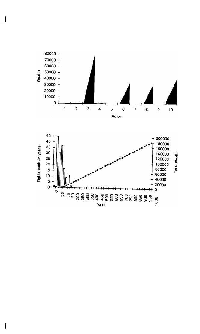
134
C H A P T E R 6
Figure 6-3. Wealth of Each Actor over 1,000 Years (Population 2)
Figure 6-4. Fights (bars) and Population Wealth (line) in Population 2.
while decreasing its commitment (if any) to 3 and 4. In general, as fights
take place, they increase the commitments of those fighting on the same
side, and decrease the commitments of those fighting on opposite sides.
Thus, as clusters begin to form, they tend to get ever more distinct. This is
because pairs of actors who fought together became even more commit-
ted to each other, and pairs on opposite sides lost whatever partial com-
mitment they may have had to each other. By year 45, fights were taking
place that involved all ten actors, leading to the pattern of two strong and
distinct clusters that was shown in Table 6-2.
Having seen how commitments can lead to clusters in an illustration
from population 2, let us now return to the unusual case of population 1,
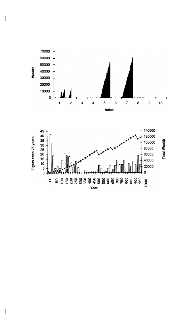
B U I L D I N G N E W P O L I T I C A L A C T O R S
135
Figure 6-5. Wealth of Each Actor over 1,000 Years (Population 3)
Figure 6-6. Fights (bars) and Population Wealth (line) in Population 3
where the strongest actor collapsed. The dynamics over the full 1,000
years was shown in Figures 6-1 and 6-2. Now we can look in detail at the
period of collapse that took place between years 890 and 950. This is
shown in Figure 6-7. In year 911, actor 10 targeted actor 9, resulting in a
“world war” involving actors 5–9 versus all the others. Actor 5, the
strongest actor, joined in even though it had minimal commitment to 9
because it had none at all to actor 10. Because 5’s commitment to 9 was
only at the 10 percent level, it contributed only 10 percent of its forces to
the fight and suffered only slightly. But later that same year, 9 again at-
tacked 10, and this time when 5 joined in, it contributed 20 percent of its
forces (having become a little more committed to 9 as well as all the
others in that alliance), and suffered a little more. Now 5 was even more

136
C H A P T E R 6
TABLE 6-1
Commitments Forming a Proximity Pattern (from Population 2, Year 25)
i
j
1
2
3
4
5
6
7
8
9
10
1
100
30
0
0
0
0
0
0
10
40
2
30
100
0
0
0
0
0
0
20
20
3
0
0
100
20
0
0
0
0
0
0
4
0
0
20
100
30
0
0
0
0
0
5
0
0
0
30
100
0
0
0
0
0
6
0
0
0
0
0
100
0
0
0
0
7
0
0
0
0
0
0
100
0
0
0
8
0
0
0
0
0
0
0
100
50
0
9
10
20
0
0
0
0
0
50
100
10
10
40
20
0
0
0
0
0
0
10
100
Note: Actors 1 and 10 are adjacent.
TABLE 6-2
Commitments Forming Pattern of Two Clusters (from Population 2, Year 50)
i
j
1
2
3
4
5
6
7
8
9
10
1
100
100
70
0
0
0
0
100
100
100
2
100
100
100
0
0
0
0
100
100
100
3
70
100
100
0
0
0
0
100
90
70
4
0
0
0
100
100
60
100
0
0
0
5
0
0
0
100
100
100
100
0
0
0
6
0
0
0
60
100
100
100
0
0
0
7
0
0
0
100
100
100
100
0
0
0
8
100
100
100
0
0
0
0
100
100
100
9
100
100
90
0
0
0
0
100
100
100
10
100
100
70
0
0
0
0
100
100
100
Note: Actors 1 and 10 are adjacent.
committed to everyone in its emerging cluster of 5–9. In years 915–918
there were five more “world wars” with the same alignments (although
different demanders and targets). As both sides became more committed
to the members of their own emerging clusters, more and more forces
were committed and more and more damage was done. The result was a
sharp decline in the wealths of the largest actors (5 on one side and 2 and
4 on the other).
This dramatic decline of the strongest actor is due to its being dragged
into fights involving weak actors to whom it had developed commit-

B U I L D I N G N E W P O L I T I C A L A C T O R S
137
TABLE 6-3
Development of Cluster of Commitments
(Fights and payments involving individual 5 of population 2
between years 25 and 50)
Year
Active
Actor
Target
Actor
Roles
Commitment
with Actor 5
Increases
a
Commitment
with Actor 5
Decreases
b
30
4
5
- - a AD - - - - -
3, 4
30
6
5
- - - - P R - - - -
6
32
3
4
- - AD d - - - - -
4
3
32
4
5
- - a AD d - - - -
6
3, 4
33
4
3
- d DA a - - - - -
4
2, 3
34
5
7
- - - - R - P - - -
7
35
5
4
- - d DA a a - - -
6, 7
3, 4
36
3
4
- a AD d - - - - -
7
2, 3
36
8
7
a a - - d d DA a a
6, 7
1, 2, 8–10
37
6
5
- - - - P R - - - -
6
38
8
7
a a a - d d DA a a
6, 7
1–3, 8–10
38
2
7
a A a - d d D a a a
6, 7
1–3, 8–10
41
8
7
a a a - d d DA a a
6, 7
1–3, 8–10
42
6
5
- - - - P R - - - -
6
42
5
4
- - - P R - - - - -
4
44
5
7
- - - - R - P - - -
7
46
7
8
d d d a a a AD d d
4, 6, 7
1–3, 8–10
47
7
8
d d d a a a AD d d
4, 6, 7
1–3, 8–10
48
7
3
d d D a a a A d d d
4, 6, 7
1–3, 8–10
48
5
3
d d D a A a a d d d
4, 6, 7
1–3, 8–10
Key to roles:
A
⫽ attacker,
a
⫽ attacker’s ally,
D
⫽ defender,
d
⫽ defender’s ally,
P
⫽ payer,
R
⫽ receiver of tributer.
a
Increases by 10 percent, up to 100 percent.
b
Decreases by 10 percent, down to 0 percent.
ments. This is reminiscent of what happened to two dominant powers,
the Hapsburgs in the seventeenth century and Britain in the nineteenth to
twentieth centuries. Paul Kennedy has an apt term for the dangers of the
excess commitments that strong powers tend to take on. It is “imperial
overstretch” (Kennedy 1987). This is just what is illustrated in Figure
6-7. It is striking that a simple model developed to generate new political
actors produced behavior that has been the subject of a major policy
debate in contemporary international affairs (e.g., Nye 1990).
Clusters are not only settings for mutual commitment; they are also
settings for extraction of tribute. The strongest actor in a cluster typically

138
C H A P T E R 6
Figure 6-7. Late Collapse of a Powerful Actor. Payments and Fights Involving
Actor 5 (Population 1, Years 890–950)
stays strong and grows by making demands on and collecting tribute
from the other members of its cluster. As actors slowly grow due to their
annual “harvest,” the strong member makes demands upon the weak
and reduces their wealth. In fact, as the strong member selects lucrative
targets, its demands automatically tend to be rotated among members of
the cluster. This rotation has the unplanned consequence of preventing
any target from growing very strong. But sometimes a weak member of a
cluster escapes demands just long enough to grow sufficiently strong to
make its own demands on still weaker members. If luck lets it be active
often enough at this critical stage, it can collect sufficient tribute so that
the strongest member no longer finds it advantageous to challenge the
newly wealthy actor. An example of this process occurred after year 100
in population 3 (see Figure 6-8). In this example, actor 5 has managed to
grow in the shadow of the strongest actor of its cluster, actor 7.
Demands within clusters do not always get resolved by payments of
tribute. In fact, civil wars can occur, that is, fighting among members of
the same cluster. The strongest member of a cluster is typically strong
enough to prevent such a fight from taking place if it took sides. If, how-
ever, the strongest member is equally committed to the attacker and the
defender (perhaps by being totally committed to both), then it would stay
neutral. This allows civil wars to occur if the active actor finds a lucrative
target within the same cluster, and the target finds it more costly to pay
tribute than to fight. The attacker and defender may even find allies
among the others if the others are not equally committed to the two sides.
Surprisingly, initial differences in wealth do not matter for wealth in

B U I L D I N G N E W P O L I T I C A L A C T O R S
139
Figure 6-8. Internal conflict. Growth of a Second Strong Actor in a Cluster of
Actors 4–8 (Population 3)
the long run. In five populations of the model there were fifty actors in
all, fourteen of whom were quite successful, using a criterion of wealth of
over 10,000 after 1,000 years. Of these fourteen successful actors, half
had less than average initial wealth and half had more than average ini-
tial wealth. One might expect that initial wealth would be a great advan-
tage because it would allow an actor to make successful demands on its
neighbors at first, and thereby build up a dominant position in a cluster.
But having substantial initial wealth can also make an actor a lucrative
target for other strong actors. In addition, having substantial initial
wealth can make one overconfident, given the limited rationality of the
decision rules in effect.
10
The results of the model’s performance can now be summarized in
terms of six characteristics:
1. Things usually do not settle down. Instead, the history of the model
shows considerable complexity. For example, as late as year 900, one of
the populations suffered a series of fights that destroyed more than three-
fourths of the global wealth (see Figure 6-2).
2. Histories show considerable variability. The combinations of
10
For example, suppose an actor with wealth of 500 makes a demand on a neighbor
with 400. The neighbor will fight rather than pay (losing 0.25 * 500
⫽ 125, which is less
than payment of the standard demand of 250). Because the target fought, the demander
loses 0.25 * 400
⫽ 100, and is worse off for having made the demand. Had the initial
wealths been greater than 1,000, this would not happen because the cost of fighting would
be greater than the standard demand of 250.

140
C H A P T E R 6
wealthy actors, frequency of fights, and trends in population wealth dif-
fer considerably from one population to another. Even though each actor
is using the same decision rules, the results differ greatly due to random
differences in initial wealth and in the order in which actors become
active.
3. “Imperial overstretch” can bring down even the strongest actor. As
an actor becomes committed to others due to tribute relationships and
fighting together, it becomes exposed to the risks of whatever fights the
others get into. Because actors decide on demands and responses based
upon their own calculations, even a weak actor can choose to make or
resist a demand for its own reasons, and thereby drag into the struggle a
strong actor who is committed to it.
4. Civil wars can occur among the smaller members of a cluster. Al-
though the strongest member of a cluster can typically prevent a fight
among members of the same cluster by taking sides, it would not do so if
it had equal commitment to the two sides. Therefore, smaller members a
cluster may fight each other while the strongest member stands aside.
5. A cluster can have more than one powerful member. Clusters are
often like empires, with one powerful actor and many weaker ones who
pay tribute to it. But as we have seen in the case of Figure 6-8, it is also
possible for a second actor to grow strong in the shadow of the first.
6. Initial endowment does not guarantee or even predict success. Be-
fore clusters of commitments are established, wealth can be as much a
handicap as an asset. The reason is that wealth makes an actor a lucrative
target for other strong actors, and can make one overconfident in making
demands.
Have New Actors Emerged?
Returning to the original goal of the project, we can now assess the ex-
tent to which the emergent clusters of mutually committed actors are
really new actors at a higher level of organization. Recall that a cluster is
defined as a set of actors who are each committed to the others at a level
of at least 50 percent. This definition provides a set of candidates who
may or may not be emergent political actors. To see if clusters actually
behave as newly emergent political actors, we return to the original set of
criteria:
1. Effective control over subordinates
a. In the simulation, clusters exhibit no rebellion. There were no fights
in a cluster against the strongest member. Note that this result is not built into
the model’s assumptions. After all, it would certainly be possible for several

B U I L D I N G N E W P O L I T I C A L A C T O R S
141
members of a cluster to join in attacking the strongest member. (There were,
however, some fights among the secondary actors within a cluster, tolerated by
the strongest.)
b. Independent “foreign policy” occurred on only rare occasions. On
these rare occasions, the strongest member was dragged into trouble by com-
mitment to a client (“imperial overstretch”).
2. Collective action (“all for one and one for all”)
a. The strong did protect the weak.
b. Members of a cluster did act together with respect to outsiders, both
in attack and defense.
3. Recognition by others as an actor did occur, since joint action of clusters
was foreseen and taken into account by outsiders. Note that the model as-
sumes that everyone can anticipate the effect of current alliances. The fact that
clusters were stable means that the short-term calculation based on alliances
was tantamount to long-term recognition of emergent actors based upon stable
clusters.
In sum, the tribute model did produce clusters of mutual commitment,
and these clusters did exhibit to a high degree all the attributes of an
emergent new political actor. In fact, even the exceptions reflected the
kind of exceptions present in international affairs, as illustrated by impe-
rial overstretch.
Variations of the Model
One of the advantages of a simulation model is that it is relatively easy to
answer “what if ” questions about the effect of varying the parameters or
the premises of the model. Here is a very brief sample of some of these
questions, with answers based on further simulation runs:
1. Does the model settle down after 1,000 years? No. Even in runs up
to 10,000 years there are repeated large wars, and strong actors continue
to rise and fall.
2. Are there better decision rules? Yes. An example is adding a con-
straint so that a demand will not be made of a target who would find it
cheaper to fight than to pay. An individual using this revised rule does
much better than the others. Moreover, if everyone is using the revised
rule, any single individual who uses the old rule does worse than the
others.
3. Does it pay to give and receive commitments? Yes. An actor who
neither gives nor receives commitment does very poorly. Moreover, if just
one actor gives and receives commitments (and the others do not, except
with that actor), then that actor does very well.
4. What happens if everyone can reach everyone else (as in sea power)?

142
C H A P T E R 6
In this extreme case, a single powerful actor tends to dominate, and there
are relatively dense patterns of commitment. Presumably, in a two-
dimensional space, where everyone has more neighbors than in a one-
dimensional space but fewer than in the “sea power” case, there might be
an intermediate level of dominance and density of commitment.
5. What if wealth does not enter into anyone’s calculations? If the de-
mands are made without regard to wealth, and if everyone always fights,
then the result is two clear clusters, one of which has virtually all the
wealth.
6. Do “islands of commitment” grow? Yes. If two adjacent actors ini-
tially have just 10 percent commitment to each other (and all other com-
mitments are zero), then these two actors develop complete commitment
to each other, and both tend to prosper.
Conclusion: Building Stepping Stones to Theory
The tribute model provides an existence proof that it is possible to use
simple local rules to generate higher levels of organization from elemen-
tary actors. In particular, it shows that a dynamics of “pay or else” com-
bined with mechanisms to increase and decrease commitments can lead
to clusters of actors that behave largely according to the criteria for inde-
pendent political states.
Like most simulation models, the tribute model generates huge
amounts of historically rich data. Indeed, a major challenge in any simu-
lation study is to find ways of analyzing and presenting data that help us
see the forest for the trees. The present essay illustrates four different
kinds of historical analysis. In effect, these are four different ways of
looking at history.
a. history from the point of view of a single actor: plots of relative wealth of
individual actors over time,
b. history from a global point of view: joint plots of wealth and number of
fights over time,
c. history from the point of view of the emergence of new actors: commit-
ment matrixes revealing emerging clusters of actors, and
d. history as “news”: event data, including chronologies of tribute pay-
ments and wars fought between alliances.
Perhaps the most useful outcome of a simulation model is to provide
new ways of thinking about old problems. In the present case, the need to
determine whether or not the model was successful in generating new
political actors forced the specification of explicit criteria for recognizing
a new political actor should one arise. This in itself is a useful exercise. In

B U I L D I N G N E W P O L I T I C A L A C T O R S
143
addition, the same need led to the development of different ways of view-
ing history, and especially ways of analyzing the interaction among
emerging clusters of actors.
In the future it would be good to use these conceptual and statistical
developments to answer some new questions suggested by the model. For
example, the dynamics we have seen in the tribute model suggest the
following interesting questions:
a. What are the minimal conditions for a new actor to emerge?
b. What tends to promote such emergence?
c. How are the dynamics affected by the number of elementary actors?
d. What can lead to collapse of an aggregate actor?
e. How can new actors grow in the shadow of established actors?
Although no one would believe that the answers to these questions
given by the model itself would necessarily be accurate for the real world,
a realistic hope is that the concepts developed in generating the answers
for the model would be useful in providing new ways of thinking about
comparable questions in the real world. Indeed, understanding the dy-
namics of the tribute model might also suggest specific hypotheses that
could be tested with data from the real world. In addition, the study of
one model, such as the tribute model, can provide the basis for insights
into how even simpler models can be developed that might allow deeper
insights into issues of emergent political organization.
Finally, a simulation model like the tribute model can lead to insights
into where there might be policy leverage in the real world. For example,
one might be able to identify situations in which slight changes in the
system could lead to substantially improved outcomes—in terms of
fewer destructive wars or greater coordination of political action. If we
knew when minor inputs could lead to major gains, we would have valu-
able clues to consider for policy leverage in the real world—the world
where avoiding war and achieving sustainability really matter.
References
Axelrod, R. 1984. The Evolution of Cooperation. New York: Basic Books.
Axelrod, R., and D. S. Bennett. 1993. “A Landscape Theory of Aggregation.”
British Journal of Political Science 23: 211–33. Included as Chapter 4 of this
volume.
Bueno de Mesquita, B., and D. Lalman. 1992. War and Reason: Domestic and
International Imperatives. New Haven: Yale University Press.
Buss, L. W. 1987. The Evolution of Individuality. Princeton, N.J.: Princeton Uni-
versity Press.

144
C H A P T E R 6
Cusack, T. R., and R. J. Stoll. 1990. Exploring Realpolitik: Probing International
Relations Theory with Computer Simulation. Boulder, Colo.: Lynne Rienner.
Epstein, J. M. 1985. The Calculus of Conventional War: Dynamic Analysis With-
out Lanchester Theory. Washington, D.C.: Brookings.
Fontana, W. 1991. “Functional Self-Organization in Complex Systems.” In 1990
Lectures in Complex Systems, SFI Studies in the Sciences of Complexity, vol. 3,
ed. L. Nadel and D. Stein, 407–26. Redwood City, Calif.: Addison-Wesley.
Hardin, G. 1968. “The Tragedy of the Commons.” Science 162: 1243–48.
Holland, J. H. 1992. “Complex Adaptive Systems.” Daedalus 121: 17–30.
Hebb, D. O. 1949. The Organization of Behavior. New York: Wiley.
Huth, P. 1988. Extended Deterrence and the Prevention of War. New Haven:
Yale University Press.
Kennedy, P. 1987. The Rise and Fall of the Great Powers. New York: Random
House.
Lanchester, F. W. 1916. Aircraft in Warfare: The Dawn of the First Arm. London:
Constable. Key chapters reprinted as “Mathematics in Warfare.” In The World
of Mathematics, ed. J. Newman. 1956. New York: Simon and Schuster.
Minsky, M. 1985. Society of the Mind. New York: Simon and Schuster.
Nye, J. S., Jr. 1990. Bound to Lead, The Changing Nature of American Power.
New York: Basic Books.
Powell, R. 1990. Nuclear Deterrence Theory: The Search for Credibility. Cam-
bridge, Eng.: Cambridge University Press.
Schelling, T. 1960. The Strategy of Conflict. New York: Oxford University Press.
Stein, D. L., ed. 1989. Lectures in the Sciences of Complexity. Redwood City,
Calif.: Addison-Wesley.
Tilly, C. 1985. “War Making and State Making as Organized Crime.” In Bringing
the State Back In, ed. P. B. Evans, D. H. Rueschemeyer, and T. A. Skocpol,
169–91. Cambridge, Eng.: Cambridge University Press.
. 1990. Coercion, Capital, and European States, AD 990–1990. Oxford:
Basil Blackwell.

7
Disseminating Culture
This chapter deals with the fundamental question of how we become
who we are through our interactions with others. The immediate origin
of this chapter is similar to the motivation of the previous chapter: a
desire to understand how nations emerge. In the previous chapter, I fo-
cused on threats and wars as mechanisms for the development of new
political actors from the competition and collaboration of more elemen-
tary political actors. This time I wanted to study the even more funda-
mental process of how communities evolve in the first place. It seemed to
me that a key part of the process was the development of enough shared
culture so that a group of people could work well together. I recognized
that in modern times, governments themselves promote culture through
powerful mechanisms such as universal schooling and the regulation of
mass media. But I was primarily interested in how the dissemination of
culture works below and indeed before the activities of powerful govern-
ments.
1
How do people come to share enough in the way of language,
habits, beliefs, and values that they can build the basis of common insti-
tutions such as effective government?
The approach I took was to model social influence: the way people
tend to change each other in the very process of interaction. My academic
interest in social influence dates back twenty years to my concern with
how people try to persuade each other, especially in foreign policy argu-
mentation. In that context I compared and contrasted styles of British,
German, and Japanese leaders in terms of the pattern of causal beliefs
they espoused while trying to persuade others to adapt their own pre-
ferred policies (Axelrod 1976 and 1977a). I also had a long-standing
interest in how the separate parts of a person’s belief and value system
more or less fit together. This was an interest that goes back to my very
first publication, which was on the structure of public opinion on policy
issues (Axelrod 1967; see also Axelrod 1973 and 1977b).
In fact, my interest in social influence dates back even further than the
beginning of my academic career. I distinctly remember an assignment I
got when I was fourteen years old. The city council of our town, Evans-
1
I do not use the more common term diffusion of culture because in anthropology that
term has taken on connotations about the spread of supposedly “superior” (or at least
attractive) Western culture.

146
C H A P T E R 7
ton, Illinois, was considering a proposal to cross-train the police officers
and firefighters. My teacher asked us to write about whether it was a
good idea or not. The plan certainly seemed like a good idea to me be-
cause the police would learn some additional first aid skills to use if they
were the first on the scene of a fire, and the firefighters would learn some
crowd control techniques to use if they happened to be the first on the
scene. I called the local fire station to see what the people there thought.
The man who answered the phone told me, “I don’t know much about it,
but we’re all against it down here.” I was not sure just why they were all
against it (probably job security), but the response made a deep impres-
sion on me: it was possible to have an opinion based upon social influ-
ence rather than independent analysis. Moreover, one could be quite
comfortable with this method of arriving at opinions. As I thought about
it, I realized the firefighter I had talked to was perhaps more sensible than
I first thought. In many circumstances, reliance on social influence could
be a quite sensible way to reach an opinion.
The present model of social influence is the simplest model in this vol-
ume, and perhaps the most ambitious. It is the simplest in the sense that
its basic mechanism follows a simple rule that leaves no room for strate-
gic choice. It is strictly adaptive in style. It is also the simplest in that the
entire description of the context and the dynamics of the model can be
stated in two or three sentences. It is the most ambitious model in this
volume in that it deals with how our very identities are shaped: who we
are affects whom we interact with, and whom we interact with shapes
who we become.
Besides being the simplest and most ambitious model in the volume, it
is also the most surprising and the most controversial. It is the most sur-
prising in that when I simulated a population with my model, my expec-
tations were wrong as often as they were right, even though I was the one
who designed the model. In addition, one of the key results was so coun-
terintuitive that at first I thought it must have been due to a programming
error. But it was not.
2
The model is the most controversial in that I have
had the most trouble getting it published. I first sent it to the American
Political Science Review, where one reviewer said about the model, “It is
one that political scientists were educated to hate. No one makes choices.
No one seeks to influence anyone else. Change has no costs, politically or
economically. Cultural change occurs all-together in a community, with
no leaders or laggards. In sum, politics are absent.”
Nevertheless, that reviewer was “enchanted” by the manuscript and
urged its publication. The other two reviewers thought the manuscript
2
Appendix A provides an independent replication of this model and confirms its key
results.

D I S S E M I N A T I N G C U L T U R E
147
needed more politics, and urged either substantial revisions or submis-
sion to a journal in another field. I chose the latter course. I made a
variety of corrections and clarifications suggested by the reviewers, and
sent it to the American Sociological Review.
The American Sociological Review had no trouble seeing the paper as
proper sociology. The deputy editor who was assigned the manuscript
wrote, “This is one of the more interesting simulation papers I have
read,” but “I am not very enthusiastic overall about these types of pa-
pers.” The reviewers all thought the paper had real promise (each with
his or her own set of proposed revisions), and the deputy editor’s sum-
mary was “I suggest we should honor the reviewers’ advice: to invite a
revise and resubmit.”
Because the deputy editor was not enthusiastic about simulation in
general, I decided that it would be difficult to convince her to accept the
paper as long as the reviewers retained any qualms at all. Therefore I
decided to send it elsewhere.
My third try was the Journal of Conflict Resolution, known for its
interdisciplinary range. This time, one reviewer was completely positive
and the other asked only that I expand the model to include cultural drift.
With the editor’s encouragement, I gave this a try but found that the
results were so complicated that I felt unable to give a coherent account
of them. Therefore I proposed including a brief description of the diffi-
culties of dealing with cultural drift, and leaving their solution for future
research. The editor agreed, and accepted the paper with this addition to
the section on “Extensions of the Model.” The moral of the story, I sup-
pose, is that persistence pays.
References
Axelrod, Robert. 1967. “The Structure of Public Opinion on Policy Issues.” Pub-
lic Opinion Quarterly 31: 51–60.
. 1973. “Schema Theory: An Information Processing Model of Perception
and Cognition.” American Political Science Review 67: 1248–66.
. 1976. The Structure of Decision: The Cognitive Maps of Political Elites.
Princeton, N.J.: Princeton University Press.
. 1977a. “Argumentation in Foreign Policy Settings: Britain in 1918, Munich
in 1938, and Japan in 1970.” Journal of Conflict Resolution 21: 727–56.
. 1977b. “How a Schema Is Used to Interpret Information.” In Thought
and Action in Foreign Policy, ed. G. Matthew Bonham and Michael J. Shapiro,
226–41. Basel: Berkhauser Verlag.

Disseminating Culture
THE DISSEMINATION OF CULTURE: A MODEL WITH LOCAL
CONVERGENCE AND GLOBAL POLARIZATION
R O B E RT A X E L R O D
Reprinted from Robert Axelrod, “The Dissemination of Culture: A Model with Local Con-
vergence and Global Polarization,” Journal of Conflict Resolution 41 (1997): 203–26. Re-
printed by permission of Sage Publications, Inc.
Abstract:
Despite tendencies toward convergence, differences between individuals and
groups continue to exist in beliefs, attitudes, and behavior. An agent-based
adaptive model reveals the effects of a mechanism of convergent social influ-
ence. The actors are placed at fixed sites. The basic premise is that the more
similar an actor is to a neighbor, the more likely that that actor will adopt one
of the neighbor’s traits. Unlike previous models of social influence or cultural
change that treat features one at a time, the proposed model takes into account
the interaction between different features. The model illustrates how local con-
vergence can generate global polarization. Simulations show that the number
of stable homogeneous regions decreases with the number of features, increases
with the number of alternative traits per feature, decreases with the range of
interaction, and (most surprisingly) decreases when the geographic territory
grows beyond a certain size.
Maintenance of Differences
If people tend to become more alike in their beliefs, attitudes, and behav-
ior when they interact, why do not all such differences eventually disap-
pear? Social scientists have proposed many mechanisms to answer this
question. The purpose of the present essay is to explore one more mecha-
nism. The mechanism proposed here deals with how people do indeed
become more similar as they interact, but also provides an explanation of
why the tendency to converge stops before it reaches completion. It there-
I thank Chris Achen, David Axelrod, Rob Axtell, Scott Bennett, Arthur Burks, Lars-Erik
Cederman, Michael Cohen, Paul Courant, Joshua Epstein, Jay Harrington, Larry
Hirschfeld, John Holland, David Lazer, Robert Pahre, Rick Riolo, Carl Simon, and Dan
Sperber. For financial support I thank Project 2050 through the Santa Fe Institute, and the
LS&A Enrichment Fund of the University of Michigan.

D I S S E M I N A T I N G C U L T U R E
149
fore provides a new type of explanation of why we do not all become
alike. Because the proposed mechanism can exist alongside other mecha-
nisms, it can be regarded as complementary with older explanations,
rather than necessarily competing with them.
Unfortunately, there is no good term to describe the range of things
about which people can influence each other. Although beliefs, attitudes,
and behavior cover a wide range indeed, there are even more things over
which interpersonal influence extends, such as language, art, technical
standards, and social norms. The most generic term for the things over
which people influence each other is culture. Therefore, the term culture
will be used to indicate the set of individual attributes that are subject to
social influence. It should be emphasized that there is no connotation that
within a single society there is a uniform culture. In addition, the mean-
ing or significance of the elements of culture is not specified. Instead, the
question being investigated is how people influence each other on a given
set of features, and why this influence does not lead to homogeneity.
The process by which people become similar to each other or retain
their differences is central to a variety of important topics, including the
following:
1. State formation. The formation of a national state is facilitated
when its people have shared meanings and interlocking habits of commu-
nication (Deutsch 1953 and 1969). Giddens (1979) and Anderson (1991)
show how nationalism is needed by the state, and the sense of imagined
community is central to the attainment of nationalism. Thus, the process
of at least partial convergence is critical for the formation of states.
2. Succession conflicts. Although states, once formed, typically seek to
reduce internal cleavages, such cleavages often persist. Civil wars, espe-
cially wars of succession, tend to occur around unresolved conflicts in
societies, especially when the conflicts have a clear territorial basis. In-
deed, even expert observers were surprised by the extent to which lines of
fracture in the Soviet Union survived decades of state efforts to amelio-
rate them. The process by which people become similar to each other or
retain their differences is clearly vital to our understanding of how states
survive or disintegrate.
3. Transnational integration. On a larger scale, the same processes are
central to the prospects for further development of transnational institu-
tions such as the European Community, GATT, and the United Nations.
The development of international and especially transnational institu-
tions depends in large part on the extent to which norms and ease of
understanding come to be shared over territories more extensive than
boundaries of current states.
4. Domestic cleavages. It has long been recognized that the everyday
domestic politics of democracies is largely shaped by the nature of the

150
C H A P T E R 7
societal cleavages (e.g., Lipset et al. 1956; Campbell et al. 1960; Key
1961). An important question is whether such cleavages will be amelio-
rated or reinforced through local interactions (e.g., Coleman 1957; Put-
nam 1966). America’s current debate over multiculturalism is just one
example of our concern with the dynamics of cultural difference.
In addition to these specific topics, the effects of cultural change in the
broadest sense have long been central questions. Understanding how a
culture can get established, how it can spread, and how it can be sus-
tained has growing importance in today’s world. We wonder whether
English will become a quasi-universal language, whether standards for
new technologies can be established, and whether popular songs and
dress will become universal. We applaud the spread of a common culture
when it favors efficient communication, prevents unnecessary conflict,
and fosters action for global needs such as sustainable growth. On the
other hand, with the spread of common culture, we abhor the harm done
to peoples whose cultures are destroyed, the loss to the rest of us of the
wisdom embodied in these vanishing cultures, and the loss to everyone of
the adaptive potential made possible by cultural diversity.
Existing explanations for why differences are durable employ a wide
variety of mechanisms. They are all valid explanations under specific
conditions.
1. Social differentiation. Groups actively differentiate themselves from
each other (Simmel [1908] 1955). People who identify with one group
often emphasize and even promote differences with members of other
groups. In the case of ethnic groups, this differentiation can lead to
sharpening of cultural and geographic boundaries between groups (Barth
1969; Hannan 1979).
2. Fads and fashions. When people want to be different from others,
fads will come and go. When some want to be different but others want
to copy them, the result is fashion: a never-ending chase of followers
running after leaders.
3. Preference for extreme views. Tendencies toward homogeneity of
opinion can be counteracted if people tend to prefer extreme positions on
issues. This idea was first proposed by Abelson and Bernstein (1963).
Recent simulation models have shown how this mechanism can lead to
polarization and clustering (Nowak et al. 1990; Latane et al. 1994).
4. Drift. There may be random changes in individual traits. This can
lead to differentiation among subgroups. For example, languages slowly
evolve and differentiate.
5. Geographic isolation. If people move to be near others who are sim-
ilar to themselves, the result can be clustering of similar people (e.g.,
Schelling 1978). If carried to extremes, geographic or other forms of vol-
untary or imposed segregation can sustain differences by reducing inter-
actions between members of different groups.

D I S S E M I N A T I N G C U L T U R E
151
6. Specialization. People may have interests that are at least partially
resistant to social influence. This resistance has been modeled as factors
that have a persistent effect on an individual despite social influence
(Friedkin and Johnsen 1990; Marsden and Friedkin 1993).
7. Changing environment or technology. When the environment is
constantly changing, the response may be constantly changing as well. If
the environment is changing faster than people can respond to it, then
differences may persist as different people or groups change in different
ways in response to their ever-changing environment.
Despite the existence of so many mechanisms for the maintenance of
differences, none of them takes into account the fundamental principle of
human communication that “the transfer of ideas occurs most frequently
between individuals . . . who are similar in certain attributes such as be-
liefs, education, social status, and the like” (Rogers 1983, 274; see also
Homans 1950). The model of social influence offered here abstracts this
fundamental principle to say that communication is most effective be-
tween similar people. Put another way, the likelihood that a given cul-
tural feature will spread from one individual (or group) to another de-
pends on how many other features they may already have in common.
Similarity leads to interaction, and interaction leads to still more simi-
larity. For reasons that will be explored below, this process need not lead
to complete convergence. Indeed, the most interesting thing about the
model is the way it can generate few or many distinct cultural regions
depending on the scope of cultural possibilities, the range of the interac-
tions, and the size of the geographic territory.
The present model offers a new way of looking at the dynamic process
of social influence. The model is not intended to predict any particular
historical events. Instead, it is meant to show the consequences of a few
simple assumptions about how people (or groups) are influenced by those
around them.
Approaches to Social Influence
Although over a hundred definitions of “culture” have been proposed
(Kroeber and Kluckhorn 1952), everyone agrees that culture is some-
thing people learn from each other. For the present purposes, culture is
assumed to satisfy two simple premises: people are more likely to interact
with others who share many of their cultural attributes, and interactions
between two people tend to increase the number of attributes they share.
For example, a person is more likely to talk to someone who speaks a
similar language than one who speaks a dissimilar language, and the very
act of communication tends to make their future patterns of speech even
more similar. The process of social influence applies not only to language,

152
C H A P T E R 7
but also to beliefs, attitudes, and behaviors. It applies to everything from
style of dress to fundamental values, and from the adoption of Arabic
numerals to the adoption of computer standards.
Anthropologists have taken two distinct approaches to the study of
cultural change. The diffusionists treated a given culture as a set of distinct
traits, each of which could be passed along (or diffused) to another culture
(for a review, see Voget 1975). More recently, most anthropologists have
emphasized the interconnections between the many traits that make up a
culture, viewing culture as a system of symbols by which people confer
significance on their own experience (e.g., Geertz 1973). This holistic
approach stresses that the meaning of any given trait is embedded in the
whole set of relationships with other traits, and consequently that a given
culture tends to be a more or less integrated package. Unfortunately, nei-
ther approach has done much to formalize its ideas of cultural change in
formal models whose implications can be systematically explored. (For
exceptions see Renfrew 1973; Renfrew and Cooke 1979; Sabloff 1981.)
Other social scientists have provided models of how social influence
works within a given society. These models of change within a single
society also help illuminate how one group might influence another, and
hence how one culture might influence another. An early example is Cole-
man’s sociological model of the spread of smoking among teenage boys
in which friendship affects behavior and behavior affects friendship
(1965). Psychologists and sociologists have also proposed models of so-
cial influence (Nowak et al. 1990; Friedkin and Johnsen 1990; Carley
1991; Marsden and Friedkin 1993). Political scientists have built models
of attitude change in political campaigns (Putnam 1966; Huckfeldt and
Sprague 1991; Brown and McBurnett 1993). Organization theorists have
modeled social influence in formal organizations (March 1991; Harrison
and Carroll 1991). Theories about changes in beliefs, attitudes, and be-
havior have also been developed for the spread of social norms (e.g.,
Lewis 1967; Ullmann-Margalit 1977; Axelrod 1986), the spread of
knowledge (Carley 1991), the diffusion of innovations (see Rogers 1983;
Nelson and Winter 1982), and the establishment of technical standards
(Saloner and Farrell 1986; Axelrod et al. 1995).
Finally, biologists have modeled the joint contribution of genetics and
learning in social influence (Cavalli-Sforza and Feldman 1981; Lumsden
and Wilson 1981; Boyd and Richerson 1985: see also Durham 1991).
A striking fact about these models is that they treat each feature of a
culture independently of the other features.
1
1
One exception is Carley’s (1991) model of the spread of knowledge. In this model,
group differences disappear unless members of different groups initially share no knowl-
edge in common. The only other exception is the “indirect bias” model of Boyd and Richer-
son (1985), which allows the attractiveness of a cultural trait to be affected by a control
trait. But even in this model, only one cultural trait is considered.

D I S S E M I N A T I N G C U L T U R E
153
The model of social influence given in this essay is new in two regards.
First, it explicitly takes into account that the effect of one cultural feature
depends on the presence or absence of other cultural features. Second, it
takes into account that similar individuals are more likely to influence
each other than dissimilar individuals. The only other formal model that
treats culture as multidimensional does not take into account the degree
of cultural similarity in its mechanism for social influence (Epstein and
Axtell, 1996).
2
The methodology of the present study is based on three principles:
1. Agent-based modeling. Mechanisms of change are specified for local
actors, and then the consequences of these mechanisms are examined to
discover the emergent properties of the system when many actors inter-
act.
3
Computer simulation is especially helpful for this bottom-up ap-
proach, but its use predates the availability of personal computers (e.g.,
Schelling 1978).
2. No central authority. Consistent with the agent-based approach is
the lack of any central coordinating agent in the model. It is certainly true
that important aspects of cultures sometimes come to be standardized,
canonized, and disseminated by powerful authorities such as church fa-
thers, Webster, and Napoleon. The present model, however, deals with
the process of social influence before (or alongside of ) the actions of such
authorities. It seeks to understand just how much of cultural emergence
and stability can be explained without resort to the coordinating influ-
ence of centralized authority.
3. Adaptive rather than rational agents. The individuals are assumed
to follow simple rules about giving and receiving influence. These rules
are not necessarily derivable from any principles of rational calculation
based upon costs and benefits, or forward-looking strategic analysis typi-
cal of game theory. Instead, the agents simply adapt to their environment.
The Model
Culture is taken to be what social influence influences. For present pur-
poses, the emphasis is not on the content of a specific culture, but rather
2
The Epstein and Axtell “Sugarscape” model is very rich, incorporating trade, migra-
tion, combat, disease, and mating. For example, actors of similar culture are allowed to
mate, and actors of dissimilar culture are allowed to fight.
3
Agent-based models in political science have usually focused on conflict processes
(such as war and military alliances) rather than social influence. Examples are Bremer and
Mihalka (1977), Schrodt (1981), Cusack and Stoll (1990), Axelrod (1995), and Cederman
(forthcoming). Agent-based models dealing with social influence are Huckfeldt and Sprague
(1991) and Brown and McBurnett (1993). A wide-ranging agent model is Epstein and
Axtell (1996).

154
C H A P T E R 7
on the way in which any culture is likely to emerge and spread. Thus, the
model assumes that an individual’s culture can be described in terms of
his or her attributes, such as language, religion, technology, style of dress,
and so forth.
Because the model can be abstract about the specific content of an
individual’s culture, it describes a culture as a list of features or dimen-
sions of culture. For each feature there is a set of traits, which are the
alternative values the feature may have. For example, one feature of a
culture could be the color of belt that is worn, and the traits would be the
various alternative colors that might be worn in a society. To be concrete,
suppose that there are five features and each feature can take on any one
of ten traits. Then a culture can be described as a list of five digits such as
8, 7, 2, 5, and 4. In this case, the first cultural feature has the eighth of its
possible values. This abstract formulation means that two individuals
have the same culture if they have the same traits for each of the five
features. The formulation allows one to define the degree of cultural sim-
ilarity between two individuals as the percentage of their features that
have the identical trait.
The model includes a geographic distribution of individual agents. A
simple example would be a set of 100 sites, arrayed on a ten by ten grid.
Because there is no movement in the model, the sites themselves can be
thought of as homogeneous villages. These sites are the basic actors of
the model. Each site can interact only with its immediate neighbors. A
typical site has four neighbors (north, east, south, and west). Sites on the
edge of the map have only three neighbors, and sites in the corners have
only two neighbors.
Table 7-1 shows a typical starting situation with randomly assigned
cultures. As expected, most of the sites share no more than one feature
with any of its neighbors. The underlined site, however, happens to share
two features (the fourth and the fifth features) with its neighbor to the
south. Because these two sites share two of the five attributes, their cul-
tural similarity is 40 percent.
The process of social influence in the model can be described as a series
of events. The basic idea is that agents who are similar to each other are
likely to interact and then become even more similar. This is implemented
by assuming that the chance of interaction is proportional to the cultural
similarity two neighbors already have. Here, then, is the formal state-
ment of the entire dynamics of the model:
Repeat the following steps for as many events as desired.
Step 1. At random, pick a site to be active, and pick one of its neighbors.
Step 2. With probability equal to their cultural similarity, these two
sites interact. An interaction consists of selecting at random a feature
on which the active site and its neighbor differ (if there is one), and

D I S S E M I N A T I N G C U L T U R E
155
TABLE 7-1
A Typical Initial Set of Cultures
74741
87254
82330
17993
22978
82762
87476
26757
99313
32009
01948
09234
67730
89130
34210
85403
69411
81677
06789
24042
49447
46012
42628
86636
27405
39747
97450
71833
07192
87426
22781
85541
51585
84468
18122
60094
71819
51912
32095
11318
09581
89800
72031
19856
08071
97744
42533
33723
24659
03847
56352
34490
48416
55455
88600
78295
69896
96775
86714
02932
46238
38032
34235
45602
39891
84866
38456
78008
27136
50153
88136
21593
77404
17043
39238
81454
29464
74576
41924
43987
35682
19232
80173
81447
22884
58260
53436
13623
05729
43378
57816
55285
66329
30462
36729
13341
43986
45578
64585
47330
Note: The underlined site and the site to its south share traits for two of the five cultural features,
making a cultural similarity of 40 percent.
changing the active site’s trait on this feature to the neighbor’s trait on
this feature.
4
This process can be illustrated using Table 7-1. In step 1, suppose the
underlined site is selected, along with its neighbor to the south. In step 2,
the active site and its neighbor have a 40 percent chance of interacting
because they share traits for two of their five features. If they do interact,
then the culture of the underlined site would take on the trait of one of
the three features that was different in the culture of its neighbor to the
south. For example, if the first feature was the one to change, then the
value of 6 from the neighbor’s first feature would become the value of the
first feature of the underlined site, changing its culture from 82330 to
62330. This change will increase the cultural similarity of these two sites
from 40 percent to 60 percent, making it even easier for them to converge
still further.
5
Note that the activated site, rather than its neighbor, is the one that
may undergo change. This is done to guarantee that each site has an
equal chance of being a candidate for social influence, even though the
sites on the edge of the map have fewer neighbors than sites in the
interior.
4
For those who prefer symbolic statements, here is a complete description of how the
culture, c, at a site can change. Select a random site (s), a random neighbor of that site (n),
and a random feature (f). Let G(s,n) be the set of features, g, such that the cultural traits are
unequal, i.e. c(s,g)
苷 c(n,g). If c(s,f) ⫽ c(n,f) and G is not empty, then select a random
feature, g, in G(s,n), and set c(s,g) to c(n,g). This implementation of the model takes advan-
tage of the fact that the probability that a random feature, f, will have the same trait at two
sites equals the cultural similarity between those two sites.
5
The simulation is done one event at a time to avoid any artifacts of synchronous activa-
tion of the sites. See Huberman and Glance (1993).

156
C H A P T E R 7
The Emergence of Regions of Shared Culture
How do cultural regions develop? Does everyone come to share the same
culture, or do distinct cultural regions develop? Does the system settle
down, and if so, how long does it take?
To begin to answer questions like these, it pays to start with a single
run of the model over time.
6
To make the development of cultural regions
more apparent, we can shift our attention from the details of the culture
at each site to the cultural similarities between adjacent sites. These cul-
tural similarities can be represented in a map, such as the one in Figure
7-1(a). This shows the (cultural) distances between adjacent sites at the
start. Notice that most of the boundaries are drawn in black, indicating
that at most one of the five features is shared. The site marked “A” in
Figure 7-1(a) corresponds to the underlined site in Table 7-1. Notice that
the boundary between this site and the one to its south is drawn in dark
gray, indicating that the cultural similarity between them is 40 percent at
the start of the run.
The other panels of Figure 7-1 show what happens over time.
7
Time is
measured in events, representing the activation of a site. For example,
Figure 7-1(b) shows the start of the emergence of distinct cultural regions
after 20,000 events. For our purposes, a cultural region can be defined as
a set of contiguous sites with the identical culture. Notice that already at
this stage, many cultural boundaries have disappeared as some cultural
regions have grown to include four or five sites.
By 40,000 events the cultural regions have gotten bigger. In addition,
even many of the boundaries between regions are now light gray, indicat-
ing that there is only a single feature on which they differ. By 80,000
events, there are only four regions left. In fact, by 81,000 events, the
region surrounded by light gray gets completely absorbed into the largest
region, leaving only three regions. Not only that, but the remaining three
regions are completely stable because members of adjacent regions have
absolutely no features in common and hence cannot interact.
Some of the questions can now be answered about the effects of social
influence over time and space in this model.
6
The model can be regarded as a Markov process with absorbing states. Unfortunately,
the mathematical tools for analyzing Markov processes, such as eigenvalue analysis, are not
very helpful in this case because the dynamics are so complex. For example, the number of
possible states for the situation given in Table 7-1 is 10
500
, which is far more than the
number of atoms in the universe. Other agent-based models that can be regarded as
Markov processes have also had to resort to computer simulation (e.g., Bremer and Mi-
halka 1977; Schrodt 1981; and Cusack and Stoll 1990).
7
The model is coded in Pascal. Running on a Macintosh Quadra 700, the run shown in
Figure 7-1 took eleven seconds. See fn. 12 for source code availability.

D I S S E M I N A T I N G C U L T U R E
157
Figure 7-1. Map of Cultural Similarities. Note: Cultural similarity between adja-
cent sites is coded as: Black
⭐ 20%, Dark Gray ⫽ 40%, Gray ⫽ 60, Light Gray ⫽
80%, White
⫽ 100%. This run was conducted using five cultural features and ten
traits per feature, using the initial conditions shown in Table 7-1. Each interior
site has four neighbors.
1. Initially, most neighboring sites have little in common with each other,
and hence are unlikely to interact. However, when two sites do interact they
become more similar, and hence are more likely to interact in the future.
2. Over time, specific cultural features tend to be shared over a larger
and larger area. Indeed, regions start to form in which all the features are
exactly the same.

158
C H A P T E R 7
3. Eventually, no further change is possible. This happens when every
pair of neighboring sites have cultures that are either identical or com-
pletely different. If a pair are identical, they can interact but the interaction
will not cause either to change. If they are completely different, they will not
even interact. In the sample run shown in Figure 7-1, the process settled
down with exactly three cultural regions, two of which had few sites.
4. Initially, there are almost as many regions as sites, but eventually there
are only a few regions. An indication of the extent to which the process of
social influence resists complete homogenization is the number of regions
that remain when no further change is possible. The number of stable
regions can be defined as the number of cultural regions that exist when
each cultural region has nothing in common with any of the regions it is
adjacent to. In the sample run, shortly after the time shown in Figure 7-1(d),
exactly three stable regions survived, two of which had few sites.
5. In retrospect, the origins of the stable cultural regions can be seen
far back in history.
8
For example, the cultural region of four sites in the
southeast corner of Figure 7-1(d) can be clearly discerned as far back in
time as Figure 7-1(b). However, looking just at the map of cultural simi-
larities at that early time would not allow one to know which of the
many cultural regions that existed then would survive.
The Number of Stable Regions
For society, an important question is how many cultural regions will sur-
vive. Although all social influence in the model involves convergence be-
tween neighbors, the process of convergence can stop with several surviv-
ing cultural regions, each of which is completely different from the
adjacent cultural regions.
In the sample run, three cultural regions survived. This is fairly typical of
runs done under identical conditions but with different random choices. In
a set of 100 runs of this type, the median number of stable regions was
three. But there was also quite a bit of variation. In 14 percent of the runs
there was only one stable region, while in 10 percent of the runs there were
more than six.
Scope of Cultural Possibilities
The model can be used to explore how the number of stable regions
depends on various factors such as the scope of cultural possibilities, the
range of the interactions, and the size of the geographic territory. First
8
This is an example of what is called path dependence (e.g., Arthur 1988).

D I S S E M I N A T I N G C U L T U R E
159
consider the scope of cultural possibilities. In the model, cultural com-
plexity depends on two things: the number of cultural features and the
number of possible traits that each feature can have. For example, in the
sample run there were five features, each with ten possible traits. A plau-
sible hypothesis is that the more variety that is possible among cultures,
the greater the number of stable regions there will be. This hypothesis
would be based on the idea that the more features and the more traits per
feature, the more cultural regions there would be at the end.
Table 7-2 shows the average number of regions that resulted from all
combinations of five, ten, or fifteen features as well as five, ten, or fifteen
traits per feature. For each combination of parameters, ten runs were
conducted. Table 7-2 shows that the original culture of five features of
ten traits each gave an average of 3.2 stable regions.
When the number of traits per feature was held at ten, but the number of
features was increased from five to ten or fifteen cultural features, the
process converged to a single stable region. Thus, as the number of features
grows, so does the likelihood of complete cultural convergence. This seems
counterintuitive at first, because one might suppose that more features
would make convergence more difficult. In fact, just the opposite is true.
The reason is that with more features, there is a greater chance that two sites
will have the same trait on at least one feature, and therefore will be able to
interact. With interaction comes the sharing of the trait on an additional
cultural feature. So with more features in the culture there is a greater
chance neighbors will have something in common, and thus they will have a
greater chance to attain complete cultural convergence with each other.
The effect of differing the number of traits on each feature is also
shown in Table 7-2. Again there is a curious result: increasing the number
of traits per feature has the opposite effect of increasing the number of
features. For example, moving from ten to fifteen traits when there are
five features actually increases the average number of stable regions from
3.2 to 20.0. When there are few features and many traits then there is a
good chance that two neighbors will share no features, and thus be un-
able to interact. This in turn makes it easier for many distinct regions to
form, each of which has no features in common with any adjacent region.
In sum, the complexity of the culture needs to be differentiated to ac-
count for the number of stable regions. Having more features (i.e., di-
mensions) in the culture actually makes for fewer stable regions, but hav-
ing more alternatives on each feature makes for more stable regions.
Range of Interaction
The next question is how the process of cultural formation is influenced
by the number of neighbors with which a site can interact. So far, each

160
C H A P T E R 7
TABLE 7-2
Average Number of Stable Regions
Number of
cultural features
Traits per feature
5
10
15
5
1.0
3.2
20.0
10
1.0
1.0
1.4
15
1.0
1.0
1.2
Note: These runs were done with a territory of 10
⫻ 10 sites, and
each interior site had four neighbors. Each condition was run ten
times.
interior site was allowed to interact with four adjacent sites. It is plausi-
ble that if interactions could occur over somewhat greater distances, the
process of cultural convergence would be made easier. The expected re-
sult would be fewer distinct regions when the process settled down.
To test this hypothesis, additional runs were conducted in which each
site could interact with other sites using larger neighborhoods, encom-
passing eight and twelve neighbors for interior sites. The neighborhoods
with eight sites consisted of the four adjacent sites plus the four diagonal
sites, making a square neighborhood. The neighborhoods of twelve sites
consisted of those eight sites plus the four sites that were two units in
each of the cardinal directions, making a diamond shaped neighborhood.
To study the effect of neighborhood size, the entire set of ten replications
of each of the nine kinds of culture was run for the neighborhood of sizes
of four, eight, and twelve.
As expected, larger neighborhoods result in fewer stable regions. Aver-
aged over the nine types of culture, small neighborhoods have 3.4 stable
regions, medium-sized neighborhoods give 2.5 stable regions, and large
neighborhoods generate only 1.5 stable regions. Thus when interactions
can occur at greater distances, cultural convergence is easier.
Size of the Territory
The final statistical question is how the outcome of social influence pro-
cess is affected by the size of the territory. In all the runs so far, the size of
the territory was 10
⫻ 10 sites. Over the nine different kinds of culture
and three different sizes of neighborhoods, there was an average of 2.5
stable regions. One would suppose that the more sites there are, the more
cultural regions result.
To test this hypothesis, additional territories were examined that were

D I S S E M I N A T I N G C U L T U R E
161
5
⫻ 5 sites, and 15 ⫻ 15 sites. A complete factorial design was done for
each of the eighty-one conditions: three sizes of territory, nine types of
culture, and three types of neighborhood. Each condition was replicated
ten times, giving 810 runs in all. The results are very surprising. In these
runs, the size of the territory had no substantial effect on the number of
cultural regions formed. Here are the averages: with small (5
⫻ 5) territo-
ries there were 2.4 stable regions, with medium (10
⫻ 10) territories
there were 2.5 stable regions, and with larger territories (15
⫻ 15) there
were 2.2 stable regions.
Clearly, a more detailed analysis of the effect of size is needed. The best
way to do this is to hold the other parameters constant. For convenience,
the other parameters can be fixed at the levels that gave the largest num-
ber of stable regions. This means few cultural features (five), many traits
per feature (fifteen), and small neighborhoods (four neighbors for inte-
rior sites). With these parameters held constant, the number of stable
regions can be determined as a function of the size of the territory.
The results are shown in Figure 7-2, which summarizes forty runs each
for territories from 2
⫻ 2 sites up to 35 ⫻ 35 sites, and ten runs each for
territories of 50
⫻ 50 and 100 ⫻ 100 sites. Consistent with the earlier
runs shown in Table 7-2 (with few features and many traits per feature),
there were about twenty stable regions in a territory of 10
⫻ 10 sites. The
overall result shown in Figure 7-2 is that the number of stable regions
increases until it reaches a maximum of about twenty-three when the
territory has 12
⫻ 12 sites. The number of stable regions then declines to
about six for a territory of 50
⫻ 50 sites and about two for a territory of
100
⫻ 100 sites.
The earlier result suggesting that territorial size did not have a substan-
tial effect on the number of stable regions can now be seen as misleading.
The earlier analysis averaged nine kinds of culture and three ranges of
interaction, leading to about the same number of stable regions no matter
whether the territory was 5
⫻ 5, 10 ⫻ 10, or 15 ⫻ 15. The results shown
in Figure 7-2, however, demonstrate that when the type of culture and the
range of interaction is held constant, the number of stable regions is very
sensitive to the size of the territory: both small and large territories have
few stable regions, whereas moderate-sized territories have the largest
number of stable territories.
Why do moderate-sized territories have the largest number of stable
territories? It is no surprise that smallest territories have the fewest stable
regions. After all, small territories simply do not have enough sites to
contain many different cultures. So it is not surprising that as the size of
the territory increases from, say, 2
⫻ 2 sites to 12 ⫻ 12 sites, the number
of stable regions increases. What is really surprising is that as the size of
the territory increases further, the number of stable regions actually de-
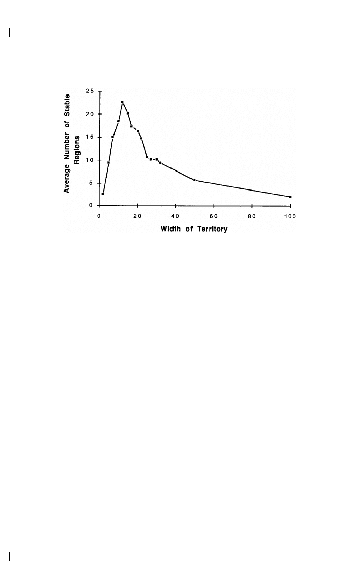
162
C H A P T E R 7
Figure 7-2. Average Number of Stable Regions. Note: The parameters for these
runs are five cultural features, fifteen traits per feature, and four neighbors for
interior sites. Each territory size was replicated forty times, except the territories
with 50
⫻ 50 sites and 100 ⫻ 100 sites, which were replicated ten times.
creases. So the interesting question is: why do large territories have fewer
stable regions than moderate-sized territories?
The result is so surprising that one might wonder whether it is due to a
programming error. Fortunately, this explanation can be ruled out. The
present simulation model has been independently implemented by an-
other team in what is apparently the first systematic effort to align two
related agent-based simulation systems (Axtell et al. 1996). The key re-
sults of the present model were confirmed.
One might also wonder whether the phenomenon of large territories
having fewer stable regions has something to do with the existence of
boundaries on the territories. Boundaries can be eliminated by wrapping
around the northern and southern edges, and the eastern and western
edges. Simulations with this neighborhood topology show the same pat-
tern as before: the number of stable regions increases for a while as the
size of the territory increases, but then declines. Although the peak occurs
earlier (i.e., with somewhat smaller territories) and is not as high (i.e.,
with somewhat fewer stable regions), the shape of the curve is similar to
the one in Figure 7-2. So the existence of territorial boundaries is not the
cause of large territories having fewer stable regions than moderate-sized
territories.

D I S S E M I N A T I N G C U L T U R E
163
To see why larger territories have fewer stable regions, it is useful to
examine what happens over time in runs of various sizes.
Analysis of Histories
Dialects
To understand the historical development of social influence in this
model, it pays to examine an artificially constructed illustration where
there are just two cultural regions, differing in a single feature. I use the
term “dialects” to describe two such similar cultures. To keep things re-
ally elementary, suppose there are just six sites on a line from west to east,
and the neighbors of each site are the adjacent sites. (See Table 7-3.)Sup-
pose, further, that the four on the west have the same culture, namely
11111, whereas the two sites on the east have culture 11112. If the acti-
vated site and its selected neighbor are both within the same region, no
change would occur, because there would be no cultural difference to
transmit. Thus, the only possibility for change would be if the active site
was in one region and its selected neighbor was in the other. The conse-
quence would be that the boundary between the two regions would move
by one site, either to the east or to the west. Moreover, these two possi-
bilities are equally likely. The next time a social influence takes place, the
regional boundary will move again, and once again there is an equal
chance the boundary will move to the east as to the west. The movement
of the regional boundary follows a process known as a random walk
with absorbing barriers (e.g., Kemeny et al. 1966, 283). In this illustra-
tion, stability will be reached when the boundary between the regions
moves all the way to the east or to the west, that is, when one dialect has
completely “eaten” the other dialect.
An interesting thing about this illustration is that the larger region is
more likely to “eat” the smaller region than the other way around. The
reason is that the random walk of the boundary is more likely to reach
the nearer edge of the map before it reaches the further edge. Thus, the
majority culture is more likely to survive than the minority culture, even
though there is absolutely no bias in the process of social influence. This
brings to mind the effort at universities and elsewhere to protect the di-
versity of a multicultural society.
This result that large regions tend to “eat” small regions can help ex-
plain what happened toward the end of the run shown in Figure 7-1.
Recall that after 80,000 events there were four regions, one of which
differed from the largest region in a single cultural feature (see Figure
7-1(d)). Once history got to this stage, the small dialect with just four

164
C H A P T E R 7
TABLE 7-3
An Illustration of Social Influence between Dialects
a. Suppose there are two regions in a territory of 6x1 sites. Suppose the
regions are dialects, differing in a single feature. Suppose one region has four
sites while the other region has two sites:
11111 11111 11111 11111 11112 11112
b. Since most sites are identical to all of their neighbors, there are only two
possibilities for social influence. These two possibilities are equally likely:
i. The fourth site is activated and borrows from the fifth site, moving the
regional boundary to the west.
11111 11111 11111 11112 11112 11112
ii. The fifth site is activated and borrows from the fourth site, moving the
regional boundary to the east.
11111 11111 11111 11111 11111 11112
c. Eventually, the process will stop when one dialect or the other is eliminated.
More likely, the 11111 dialect will eliminate the 11112 dialect because it
started with more sites.
sites was much more likely to become extinct than the large dialect,
which has ninety-one sites. Notice that as long as the sites in the other
two small regions had nothing in common with any of their neighbors,
they would not change. The possibility for social influence ended when
the larger dialect “ate” the smaller dialect, resulting in just three stable
regions.
The idea of dialects of similar cultures leads to the idea of cultural
zones of similar regions. This in turn can help unravel the puzzle of why
large territories have few stable regions.
Cultural Zones
Recall that a cultural region is a set of contiguous sites with identical
cultures. A related idea is a cultural zone: a set of contiguous sites each of
which has a neighbor with a “compatible” culture. Cultures are compati-
ble if they have at least one feature in common. This means that neigh-
boring sites with compatible cultures can interact. Thus, although the
sites in a single cultural zone may include many different regions, each of

D I S S E M I N A T I N G C U L T U R E
165
the regions in a zone is able to interact with adjacent regions in the same
zone.
9
To see how zonal and regional boundaries develop over time in a rela-
tively small territory, let us return to the run illustrated in Figure 7-1. In
Figure 7-1(d) there are four regions. However, there are only three zones,
as indicated by the black boundaries between adjacent sites, that have no
features in common. The run ends when no further change is possible,
and this happens when each zone has exactly one region, since that im-
plies that sites in different regions can no longer interact. In the run
shown in Figure 7-1, stability was reached when the small dialect was
“eaten” by the largest region. The resulting three regions correspond ex-
actly to the three zones of Figure 7-1(d). Going back in history to Figure
7-1(c), there were dozens of regions but exactly the same three zones. In
fact, this is a common historical pattern, with the zones developing be-
fore the regions. Thus the number of zones provides an early indication
of just how many stable regions there will be.
Figure 7-3 shows how the number of regions and zones develop over
time in a single run with a very large (100
⫻ 100) territory with 10,000
sites.
10
Initially, the number of regions is virtually the same as the number
of sites because it is very unlikely that two adjacent sites will have each of
their five features be equal when there are fifteen possible traits for each
feature. However, even at the start there are fewer zones than regions
because many sites will have at least one feature in common with at least
one neighbor. As Figure 7-3 shows, the number of regions declines gradu-
ally until there are about a thousand regions, and then declines in stages
until there are only two regions. On the other hand, the number of zones
declines quickly to just two. As mentioned above, when the number of
regions equals the number of zones, no further change is possible. It is
striking that it takes more than four times as long for the stable regions to
be determined than for the final number of zones to form. So most of the
history of the run was spent with many compatible cultures “struggling for
survival” within just two cultural zones, until finally only a single culture
survived in each zone. Because one of the final two zones has only one site,
all of this “struggle” took place over the 9,999 sites of the other final zone.
9
Technically, two sites are in the same zone if there is a path of adjacent sites from one
to the other such that each site has at least one feature in common with the next one on the
path.
10
Note that for Figure 7-3, the parameters were chosen to generate relatively large
numbers of stable regions. With these parameters, the average number of stable regions in
10
⫻ 10 territories was about 18.6, whereas in 100 ⫻ 100 territories, the average was only
2.1. (See Figure 2. The slight discrepancy for the number of stable regions in the 10
⫻ 10
territory in Figure 7-2 compared to the corresponding cell in Table 7-1 is due to averaging
over different runs.)
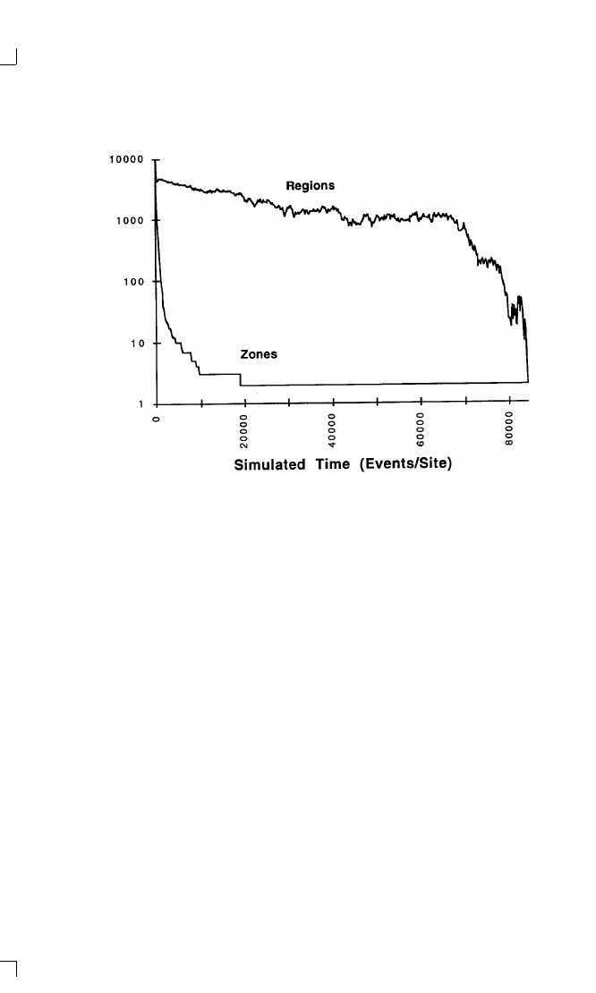
166
C H A P T E R 7
Figure 7-3. Number of Cultural Regions and Cultural Zones over Time in a Run
with a Large Territory. Note: The territory is 100
⫻ 100 sites. The other parame-
ters are as in Figure 7-2. Note logarithmic scale.
Dissolution of Cultural Boundaries
Over time, boundaries between regions in the same cultural zone tend to
dissolve. For example, if two adjacent sites share three of their five cul-
tural features, there is a good chance that they will interact and then
share four features. Then they may interact again and come to share all
five of their features. Of course, things are more complex than this be-
cause either of the two sites might also interact with others, and this
might actually decrease the cultural similarity between them. But on aver-
age, cultural similarity between adjacent sites in the same cultural zone
tends to increase.
On the other hand, adjacent sites in different cultural zones cannot
interact because they have no cultural features in common. This is why
boundaries within cultural zones tend to dissolve, but boundaries be-
tween cultural zones tend to be stable. Nevertheless, even boundaries
between cultural zones can dissolve. A boundary between two cultural
zones can dissolve if a site on the zonal boundary adopts a trait for a

D I S S E M I N A T I N G C U L T U R E
167
feature from another region in its zone. If this newly adopted trait hap-
pens to match the corresponding feature of a neighboring site from the
other zone, then the zonal boundary will begin to dissolve. This accounts
for how the number of cultural zones decreases over time, as shown in
Figure 7-3.
Another way of looking at the dynamic process is to consider how
alternative traits for a cultural feature move around in a zone as neigh-
boring sites interact. As long as there are many regions within each zone,
there are different cultural traits for at least some of the features in the
zone. As these traits move around in the zone through interactions, they
have a chance of dissolving boundaries, both regional and zonal. The net
effect is that the more time it takes for a territory to settle down, the more
chance there is that zonal as well as regional boundaries will be dissolved.
Large territories take much longer to reach stability than smaller terri-
tories, and this gives the regional and even zonal boundaries in large
territories more opportunities to dissolve. This is true even though in
comparing territories of different sizes, simulated time should be mea-
sured in events per site rather than simply events. The reason why time is
measured in events per site is that in reality various sites might be active
at virtually the same time.
Just how does time to stability vary as a function of territorial size?
Over a great range of territories, from four to 10,000 sites, the time to
stability is almost exactly proportional to the number of sites in the terri-
tory. For example, with 1,024 sites (in a 32
⫻ 32 territory), each site
needs an average of 10,036 events to reach stability. When there are
about 2.5 times as many sites (in a 50
⫻ 50 territory), about 2.5 times as
many events per site are needed to reach stability (or 25,900 events). As
the number of sites doubles, each site has twice as many chances to be
active before stability. Therefore, doubling the number of sites in a terri-
tory allows four times as many activations in all. This in turn provides
many more opportunities for boundaries to dissolve, eventually reducing
the number of regions that will still exist when no further change is pos-
sible. (By the way, to do a run of a 100
⫻ 100 territory, each site needs a
little over 100,000 events before stability is reached. Because there are
10,000 sites, a single run of this size requires simulating a billion events.)
In sum, combining an analysis of dialects, cultural zones, and the dis-
solution of cultural boundaries helps explain how territorial size deter-
mine the number of stable regions. In small territories there is not much
room for many stable regions. In moderate-sized territories there is
enough room. In large territories, there is even more room, but the pro-
cess of social influence and the consequent movement of cultural alterna-
tives goes on so long that virtually all of the cultural boundaries eventu-
ally dissolve.

168
C H A P T E R 7
Discussion
Perhaps the most important lesson of the social influence model is that
intuition is not a very good guide to predicting what even a very simple
dynamic model will produce. The social influence model is very simple
indeed. Its mechanism can be stated in a single sentence: with probability
equal to their cultural similarity, a randomly chosen site will adopt one of
the cultural features of a randomly chosen neighbor. That’s it. Yet, it
turns out to be very difficult to anticipate how the number of stable cul-
tural regions varies as a function of the four parameters in the model.
Two of the results were intuitively obvious, but two were not. The two
results that were intuitive were that the number of stable regions in-
creases with the number of possible traits that each cultural feature could
take, and decreases with the range of interaction. The two counterintui-
tive results are that the number of stable regions decreases with more
cultural features, and with large territories. The computer runs of the
social influence model demonstrate that unaided intuition about how dy-
namic processes develop over time is not necessarily very reliable.
The social influence model also illustrates how new distinctions are
suggested by a formal model. The model demonstrates that two different
aspects of cultural complexity work in opposite directions. More cultural
features lead to fewer stable regions, but more traits on each feature lead
to more stable regions. Thus, in considering the complexity of a cultural
system, one should distinguish between the number of different features
and the number of traits that each feature can take.
The social influence model also suggests that functionalist explana-
tions for common observations need not be the only or even the simplest
ones. For example, suppose there are two equally attractive variants of a
cultural practice, and the less common one vanishes over time. A func-
tionalist explanation would be that those practicing the less common
variant switched to the more common variant because there was some
advantage in doing things the way most other people do. This makes
good sense for problems of coordination, such as which side of the street
to drive on, or which technical standard to employ (Lewis 1967; Saloner
and Farrell 1986; Axelrod 1995). But, as we have seen, the social influ-
ence model demonstrates that even if there is no advantage to adopting
the majority practice, the majority practice may still tend to drive the
minority practice to extinction. The reason is that if neighbors following
different practices are equally likely to switch to the other practice, the
practice with the fewest followers is the one most likely to become extinct
first. Thus the mere observation that a practice followed by few people
was lost does not necessarily mean either that the practice had less intrin-

D I S S E M I N A T I N G C U L T U R E
169
sic merit or that there was some advantage in following a more common
practice. As in the social influence model, it could be that even unbiased
changes in adherence lead to a less common practice disappearing simply
because it is more vulnerable to random fluctuations in numbers of
adherents.
The results of the social influence model suggest two other warnings
about potentially false conclusions from empirical observations. Polar-
ization occurs in the model even though the only mechanism for change
is one of convergence toward a neighbor. Thus, when polarization is
seen, it need not be due to any divergent process. Likewise, when cultural
traits are highly correlated in geographic regions, one should not assume
that there is some natural way in which those particular traits go to-
gether. The social influence model shows how homogeneous cultural re-
gions can arise without any intrinsic relationship between the separate
dimensions that become correlated.
The social influence model suggests new empirical questions and hy-
potheses. For example, the model predicts that large territories will actu-
ally have fewer stable regions than moderate-sized territories. I have been
able to find only one relevant empirical study. This was a study of the
number of languages on the various Solomon Islands (Terrell 1977). It
found that islands with less than 100 square miles had a single language.
Above that size, the number of languages increases about one for every
190-square-mile increment in island area. This is clearly a different result
than predicted by the social influence model. Two reasons for the discrep-
ancy are suggested by the empirical study itself: languages tend to diverge
in large islands, and there is greater ecological diversity in large islands.
The social influence model ignores both of these effects. Thus, a remain-
ing unanswered question is what would happen to the number of distinct
cultures as a function of territory when there is no systematic divergence,
and when the territory is uniform.
Extensions of the Model
One advantage of a very simple model is that new things can be added
without cluttering it up very much. The following are examples of poten-
tially interesting extensions to the present model of social influence: cul-
tural drift (modeled as spontaneous change in a trait), terrain effects
(some pairs of adjacent sites less likely to interact than others), early
geographic differences (nonrandom initial traits), status (some sites less
likely to change than others), cultural attractiveness (some traits less
likely to change than others), technological change (continuing introduc-
tion of new and more attractive traits), material basis for culture (interac-

170
C H A P T E R 7
tion between trait attractiveness and terrain), public education and
broadcasting (some interactions come from widely disseminated mes-
sages), mobility,
11
organizational culture (substituting hierarchical for
geographic neighborhoods), sociology of science (interaction among
semi-isolated disciplines with drift, technological change, and organiza-
tional culture), and cultural divergence (interaction between dissimilar
sites causing increasing cultural distance).
Perhaps the most interesting extension and, at the same time, the most
difficult one to analyze is cultural drift. Cultural drift is involved in phe-
nomena such as linguistic shifts and religious fragmentation. It could also
be used to take account of the fact that there is always some chance that
neighbors will affect each other no matter how different their cultures.
Although it is easy to introduce cultural drift, analyzing its full implica-
tions is challenging. In the original version of the model, the cultures in
any given run eventually stop changing. This happens when every pair of
neighboring sites have cultures that are either identical or completely dif-
ferent. When this occurs, the resulting cultural regions are stable, and the
number of stable regions can be used as a measure of the heterogeneity of
the population.
When cultural drift is introduced, however, social influence continues
indefinitely and thus any regions that do form are not stable. This raises
two questions about how to analyze the effects of cultural drift. The first
question is: what is the best measure of the heterogeneity of the popula-
tion when a simple count of stable regions cannot be used? The second
question is: how long should a given run be allowed to go before the
measurements are taken?
In answer to the first question, there are at least four plausible mea-
sures of heterogeneity of the population at any given time. Taking a local
view, one could consider differences between all pairs of neighboring
sites. Then one could either measure how many features differed between
neighbors or count the number of neighboring pairs that had any differ-
ences. Alternatively, one could take a more global view and count the
number of cultural regions or zones that existed at a given time, even
though they were not stable.
In answer to the second question, there are two plausible ways to de-
cide when the measurements should be taken. One way is to use a given
amount of “historical” time, regardless of the number of sites in the terri-
tory. This would entail using a given number of expected activations per
site. The other method would be to run the model until a selected mea-
11
The fact that larger neighborhoods result in fewer stable regions suggests that mo-
bility will also result in fewer stable regions. This is confirmed in simulations using the
present model reported by Axtell et al. (1996).

D I S S E M I N A T I N G C U L T U R E
171
sure of heterogeneity no longer changed very much over time. This would
allow the necessary time for each territory to achieve an equilibrium be-
tween the forces of social convergence and the forces of cultural drift.
This method would presumably require more “historical time” for large
territories than small territories.
After a measure of heterogeneity and a duration method are selected,
the model can be run with cultural drift. In particular, the effects of all the
parameters can be studied and compared to their effects in the original
model. These parameters include the number of cultural features, the
traits per feature, the number of neighbors for each interior site, and the
size of the territory. Preliminary analysis suggests the effects of changes in
the parameters are quite complicated. For example, at a given rate of
cultural drift, the effects of some of the parameters seem to depend on
just which measure of heterogeneity is being used. Moreover, there are
statistical interactions among the effects of the various parameters. Fi-
nally, a complete analysis would also require varying the rate of cultural
drift as well as the parameters of the original model. In sum, it is not
trivial to determine how the introduction of cultural drift affects cultural
change in the present model of social influence.
12
Conclusion
The proposed model shows how individual or group differences can be
durable despite tendencies toward convergence. It treats culture as the
attributes that social influence can influence. Unlike previous models of
cultural change or social influence, this one is based on the interplay
between different dimensions or features that characterize people. The
basic assumption is that the opportunity for interaction and convergence
is proportional to the number of features that two neighbors already
share. Stable cultural differences emerge as regions develop in which ev-
eryone shares the same culture, but have nothing in common with the
culture of neighboring regions.
The degree of polarization is measured by the number of different cul-
tural regions that exist when no further change is possible. Theoretical
and statistical analysis shows that polarization increases when there are
few dimensions to the culture, when there are many alternative traits on
each dimension, and when interactions are only with adjacent sites.
Moreover, polarization is highest when the size of the territory is big
12
For those wishing to explore this and other extensions of the model, the source code and
documentation are available on the Internet at http:/ /pscs.physics.lsa.umich.edu/Software/
ComplexCoop.html. At that site, use the link to “Disseminating Culture.”

172
C H A P T E R 7
enough to allow for many cultures, but small enough for the change pro-
cess to settle down before all cultural boundaries are dissolved by the
spread of cultural traits.
The proposed model is unique not only in considering the interplay
between different features of culture, but also in regarding each feature as
having a whole set of alternatives. Previous models of social influence
treat culture as either a continuous dimension or a single pair of alterna-
tives. If culture is seen as a continuous dimension, then convergence tends
to lead to homogeneity unless some other mechanism is introduced to
prevent it. If culture is seen as one variable with a single pair of alterna-
tives, only two possibilities are open. Even if a set of binary alternatives is
allowed (e.g., Epstein and Axtell 1996), then the present model would
yield no more than two different cultures among its stable regions.
13
Thus, to sustain cultural variety in the proposed model, there must be
several dimensions to the culture, and each dimension must have more
than two alternative traits.
The social influence model illustrates three fundamental points:
1. Local convergence can lead to global polarization.
2. The interplay between different features of culture can shape the process
of social influence.
3. Even simple mechanisms of change can give counterintuitive results, as
shown by the present model, in which large territories generate surprisingly
little polarization.
The model suggests some interesting interpretations for the four topics
mentioned at the start of the paper. Of course, a simple model can only be
suggestive and can never be definitive.
1. State formation. Because the formation of a national state is facili-
tated by social convergence over a territory (Deutsch 1953 and 1969;
Cederman forthcoming), the results of the model demonstrate how arbi-
trary the actual boundaries can be. For example, if the political process
took hold at the historical era represented by the third panel of Figure
7-1, a state would be more likely to form in the relatively homogeneous
southern part of the map than in the relatively heterogeneous northern
part, even though there was initially nothing to distinguish north from
south. In technical terms, the outcome is highly path dependent (e.g.,
Arthur 1988).
2. Succession conflict. Cultural assimilation of multinational states has
turned out to be much harder than most observers had predicted before
13
With two traits per feature, the only stable outcome would be for every site to have
either the same culture or the complementary culture of each of its neighbors. Because the
complement of a complement is the original culture, at most two different cultures would
be possible among all the stable regions.

D I S S E M I N A T I N G C U L T U R E
173
the breakup of the Soviet Union and Yugoslavia. The model of social
influence offered here suggests how local interaction can lead to cohesive
communities without actually leading to homogenization over large dis-
tances. The model helps explain how terrain that discourages long-
distance interaction (as in the physically rugged territory of the Caucasus
or of the former Yugoslavia) promotes small-scale homogeneity along
with large-scale diversity.
3. Transnational integration.
a. The model throws an interesting light on the effect of centuries-
long European expansion to dominate much of the globe. It is not sur-
prising that increasing a cultural area homogenizes the newer additions
to the old. It is more surprising that the old regions should homogenize
internally. In other words, the model suggests that the expansion of Eu-
ropean influence from the fifteenth century could help homogenize Eu-
rope itself.
b. With recent advances in transportation, mass media, and infor-
mation technology, many interactions are now largely independent of
geographical distance. With random long-distance interactions, the het-
erogeneity sustained by local interaction cannot be sustained.
14
An inter-
esting corollary is that leaders of states can try to slow or eliminate the
homogenization by cutting their citizens off from interactions with out-
siders. Recently, however, the regimes of both Burma and North Korea
have had second thoughts about the price to be paid for such isolation.
c. The model also throws light on the controversial thesis of Hunt-
ington (1993) that conflict in the future will largely be along the bound-
aries of very large cultural regions rather than between nations within the
same cultural region. The results of the present model demonstrate that
as the relevant political territory gets larger, the number of distinct cul-
tural regions can be expected to decline, even in the absence of conquest.
4. Social cleavages.
a. Different levels of government performance in different regions
of Italy have been traced to differences in civic traditions that date back
700 years (Putnam 1993, 121–62). The interesting addition to the model
that these results suggest is that some stable civic cultures are more effec-
tive than others in promoting good government. This in turn suggests
that the role of informal organizations as the basis of social capital and
trust (Putnam 1995; Fukuyama 1995) can be analyzed in terms of how
the processes of social influence can lead to uniformity over large areas
without necessarily leading to complete homogenization.
b. The model gives the largest number of stable regions when there
14
This result was confirmed with the present model by allowing every agent to interact
with every other agent (Axtell et al. 1996).

174
C H A P T E R 7
are few cultural features and many traits per feature. This suggests that
the hardest differences to resolve through social influence are those with
few issues, but with many distinct possibilities for each issue. The surpris-
ing part of this conclusion is that having fewer issues causes such rapid
local convergence that large-scale convergence may not occur.
c. In the near future, electronic communications will allow us to
develop patterns of interaction that are chosen rather than imposed by
geography. If individuals are linked together at random, one could expect
substantial convergence over time. In the more likely case that the inter-
actions will be based on self-selection, people will tend to interact with
others who are already quite similar to them on relevant dimensions (Re-
snick et al. 1994; Abramson et al. 1988). An implication of the model is
that such self-selection could result in an even stronger tendency toward
both “local” convergence and global polarization. Only then the “local”
convergence will be based not on geography, but on emergent patterns of
more or less like-minded communication. The implications for resolving
the tensions inherent in a multicultural society are problematic.
References
Abelson, Robert, and A. Bernstein. 1963. “A Computer Simulation Model of
Community Referendum Controversies.” Public Opinion Quarterly 27: 93–
122.
Abramson, Jeffrey, F. Christopher Arterton, and Gary R. Orren. 1988. The Elec-
tronic Commonwealth. New York: Basic Books.
Anderson, Benedict. 1991. Imagined Communities: Reflections on the Origin and
Spread of Nationalism. 2d ed. London: Verso.
Arthur, W. Brian. 1988. “Urban Systems and Historical Path Dependence.” In
Cities and Their Vital Systems, ed. J. Ausubel and R. Herman, 85–97. Wash-
ington D.C.: National Academy Press.
Axelrod, Robert. 1986. “An Evolutionary Approach to Norms.” American Polit-
ical Science Review 80: 1095–1111. Included as Chapter 3 of this volume.
. 1995. “A Model of the Emergence of New Political Actors.” In Artificial
Societies: The Computer Simulation of Social Life, ed. N. Gilbert and R. Conte,
19–39. London: University College Press. Included as Chapter 6 of this
volume.
Axelrod, Robert, Will Mitchell, Robert E. Thomas, D. Scott Bennett, and Erhard
Bruderer. 1995. “Coalition Formation in Standard-Setting Alliances.” Manage-
ment Science 41: 1493–1508. Included as Chapter 5 of this volume.
Axtell, Robert, Robert Axelrod, Joshua Epstein, and Michael D. Cohen. 1996.
“Aligning Simulation Models: A Case Study and Results.” Computational and
Mathematical Organization Theory 1: 123–41. Included as Appendix A of this
volume.

D I S S E M I N A T I N G C U L T U R E
175
Barth, Fredrik. 1969. Ethnic Groups and Boundaries. Boston: Little, Brown.
Boyd, Robert, and Peter J. Richerson. 1985. Culture and the Evolutionary Pro-
cess. Chicago: University of Chicago Press.
Bremer, Stuart A., and Michael Mihalka. 1977. “Machiavelli in Machina: Or
Politics Among Hexagons.” In Problems of World Modeling, ed. Karl Deutsch
et al., 303–37. Cambridge, Mass.: Ballinger.
Brown, Thad A., and Michael McBurnett. 1993. “Emergence of Political Elites.”
Paper presented at European Conference on Artificial Life, Brussels, May
19–21.
Campbell, Angus, Philip E. Converse, Warren E. Miller, and Donald E. Stokes.
1960. The American Voter. New York: Wiley.
Carley, Kathleen. 1991. “A Theory of Group Stability.” American Sociological
Review 56: 331–54.
Cavalli-Sforza, L. L., and M. W. Feldman. 1981. Cultural Transmission and
Evolution: A Quantitative Approach. Princeton, N.J.: Princeton University
Press.
Cederman, Lars-Erik. Forthcoming. Emergent Actors in World Politics: How
States and Nations Develop and Dissolve. Princeton, N.J.: Princeton University
Press.
Coleman, James S. 1957. Community Conflict. New York: Free Press.
. 1965. “The Use of Electronic Computers in the Study of Social Organiza-
tion.” European Journal of Sociology 6: 89–107.
Cusack, Thomas R., and Richard Stoll. 1990. Exploring Realpolitik: Probing
International Relations Theory with Computer Simulation. Boulder, Colo.:
Lynne Rienner.
Deutsch, Karl W. 1953. Nationalism and Social Communication: An Inquiry in
the Foundations of Nationality. Cambridge, Mass.: Technology Press; New
York: Wiley.
. 1969. Nationalism and Its Alternatives. New York: Knopf.
Durham, William H. 1991. Coevolution: Genes, Culture, and Human Diversity.
Stanford, Calif.: Stanford University Press.
Epstein, Joshua M., and Robert Axtell. 1996. Growing Artificial Societies: Social
Science from the Bottom Up. Washington, D.C.: Brookings Institution Press;
and Cambridge, Mass.: MIT Press.
Friedkin, Noah E., and Eugene C. Johnsen 1990. “Social Influence and Opin-
ions.” Journal of Mathematical Sociology 15: 193–205.
Fukuyama, Francis. 1995. Trust. New York: Free Press.
Geertz, Clifford. 1973. The Interpretation of Cultures. New York: Basic Books.
Giddens, Anthony. 1979. The Constitution of Society. Berkeley: University of
California Press.
Hannan, Michael T. 1979. “The Dynamics of Ethnic Boundaries in Modern
States.” In National Development and the World System, ed. J. Meyer and
M. Hannan, 253–327. Chicago: University of Chicago Press.
Harrison, J. Richard, and Glenn R. Carroll. 1991. “Keeping the Faith: A Model
of Cultural Transmission in Formal Organizations.” Administrative Science
Quarterly 36: 552–82.

176
C H A P T E R 7
Homans, George C. 1950. The Human Group. New York: Harcourt, Brace.
Huberman, Bernardo A., and Natalie S. Glance. 1993. “Evolutionary Games and
Computer Simulations.” Proceedings of the National Academy of Sciences
(USA) 90: 7716–18.
Huckfeldt, Robert, and John Sprague. 1991. “Discussant Effects on Vote Choice:
Intimacy, Structure, and Interdependence.” Journal of Politics 53: 122–58.
Huntington, Samuel P. 1993. “The Clash of Civilizations?” Foreign Affairs 72:
22–49.
Kemeny, John G., J. Laurie Snell, and Gerald L. Thompson. 1966. Introduction
to Finite Mathematics. 2d ed. Englewood Cliffs, N.J.: Prentice-Hall.
Key, V. O. 1961. Public Opinion and American Democracy. New York: Knopf.
Kroeber, Alfred L., and Clyde Kluckhorn. 1952. “Culture: A Critical Review of
Concepts and Definitions.” Papers of the Peabody Museum 47: 643–44, 656.
Latane, Bibb, Andrzej Nowak, and James H. Liu. 1994. “Measuring Emergent
Social Phenomena: Dynamism, Polarization and Clustering as Order Parame-
ters of Social Systems.” Behavioral Science 39: 1–24.
Lewis, David K. 1967. Convention: A Philosophical Study. Cambridge, Mass.:
Harvard University Press.
Lipset, Seymour Martin, Martin A. Trow, and James S. Coleman. 1956. Union
Democracy. Glencoe, Ill.: Free Press.
Lumsden, Charles J., and Edward O. Wilson. 1981. Genes, Mind, and Culture:
The Coevolutionary Process. Cambridge, Mass.: Harvard University Press.
March, James G. 1991. “Exploration and Exploitation in Organizational Learn-
ing.” Organization Science 2: 71–87.
Marsden, Peter V., and Noah E. Friedkin. 1993. “Network Studies of Social Influ-
ence.” Sociological Methods and Research 22: 127–51.
Nelson, Richard R., and Sidney G. Winter. 1982. An Evolutionary Theory of
Economic Change. Cambridge, Mass.: Harvard University Press.
Nowak, Andrzej, Jacek Szamrej, and Bibb Latane. 1990. “From Private Attitude
to Public Opinion: A Dynamic Theory of Social Impact.” Psychological Review
97: 362–76.
Putnam, Robert D. 1966. “Political Attitudes and the Local Community.” Ameri-
can Political Science Review 60: 640–54.
. 1993. Making Democracy Work: Civic Traditions in Modern Italy.
Princeton, N.J.: Princeton University Press.
. 1995. “Bowling Alone.” Democracy 6: 66–78.
Renfrew, Colin. 1973. The Explanation of Social Influence: Models in Prehistory.
Pittsburgh: University of Pittsburgh Press.
Renfrew, Colin, and Kenneth L. Cooke. 1979. Transformations: Mathematical
Approaches to Social Influence. New York: Academic Press.
Resnick, Paul, Neophytos Iacovou, Mitesh Suchak, Peter Bergstrom, and John
Riedl. 1994. “GroupLens: An Open Architecture for Collaborative Filtering of
Netnews.” In Proceedings of the ACM 1994 Conference on Computer-
Supported Cooperative Work: Chapel Hill, N.C., 175–86. New York: Associa-
tion for Computing Machinery.
Rogers, Everett M. 1983. Diffusion of Innovations. 3d ed. New York: Free Press.

D I S S E M I N A T I N G C U L T U R E
177
Sabloff, Jeremy A. 1981. Simulations in Archeology. Albuquerque: University of
New Mexico Press.
Saloner, G., and J. Farrell. 1986. “Installed Base and Compatibility: Innovation,
Product Preannouncements, and Predation.” American Economic Review 76:
940–55.
Schelling, Thomas. 1978. Micromotives and Macrobehavior. New York: Norton.
Schrodt, Philip A. 1981. “Conflict as a Determinant of Territory.” Behavioral
Science 26: 37–50.
Simmel, Georg. [1908] 1955. Conflict and the Web of Group-Affiliations. New
York: Free Press.
Terrell, John. 1977. “Human Biogeography in the Solomon Islands.” Fieldiana:
Anthropology 68: 1–47.
Ullmann-Margalit, Edna. 1977. The Emergence of Norms. Oxford: Clarendon
Press.
Voget, Fred W. 1975. A History of Ethnology. New York: Holt, Reinhart and
Winston.


A P P E N D I X E S


A
Replication of Agent-Based Models
This appendix originated in an observation and suggestion by Michael
Cohen. The observation was that in order for agent-based modeling to
become a widely used tool in social science research, it will be necessary
to develop the tools for a close comparison of comparable models. This
process of close comparison or “alignment” is needed to determine
whether two modeling systems can produce the same results, which in
turn is the basis for critical experiments and for tests of whether one
model can subsume another. The suggestion was that my model of social
influence (see Chapter 7) was simple enough to serve as a good target
model for an alignment exercise, and that the Sugarscape modeling envi-
ronment of Joshua Epstein and Robert Axtell would be a good environ-
ment in which to try a “docking” experiment on alignment. I thought
Mike’s idea was a good one, so we invited Josh and Rob to join us in
performing this replication study.
This project seemed very straightforward when the four of us began,
but we found two surprising things along the way. The first was that
comparing two versions of the same model required us to develop a new
set of concepts. The second surprise was that even apparently trivial dif-
ferences in how time is handled in the model can lead to noticeable differ-
ences in outcomes, suggesting that care needs to be taken in making and
reporting these choices.
This replication study had no trouble getting published. In fact, it has
engendered substantial interest among people doing agent-based model-
ing in the social sciences because of a felt need to develop clearer stan-
dards for the emerging field.
The publication of the paper was especially useful for me. When my
social influence model was first submitted for publication, a reviewer said
that one of the reported results was so counterintuitive that additional
effort would be needed to verify that the outcome was the result of the
model rather than an error in the programming. I was happy to be able to
report back that the model had become the subject of the very first effort
to reimplement an agent-based model in a different modeling environ-
ment. Moreover, I could report that the suspicious result was confirmed
and the replication had been accepted for publication in another journal.

182
A P P E N D I X A
This methodological paper was quite effective in putting to rest one of
the objections to the substantive report of the model.
The “docking” exercise is offered as an aid to those who want to help
make agent-based modeling become part of a cumulative scientific enter-
prise. (Those who would like tips on how to undertake agent-based mod-
eling may also consult Appendix B.)

Replication of Agent-Based Models
ALIGNING SIMULATION MODELS: A CASE STUDY
AND RESULTS
R O B E RT A X T E L L , R O B E RT A X E L R O D , J O S H U A M . E P S T E I N , A N D
M I C H A E L D . C O H E N
Adapted from Robert Axtell, Robert Axelrod, Joshua Epstein, and Michael D. Cohen,
“Aligning Simulation Models: A Case Study and Results,” Computational and Mathemati-
cal Organization Theory 1 (1996): 123–41. Reprinted by permission of CMOT.
Abstract:
This essay develops the concepts and methods of a process we will call
“alignment of computational models,” or “docking” for short. Alignment is
needed to determine whether two models can produce the same results, which
in turn is the basis for critical experiments and for tests of whether one model
can subsume another. We illustrate our concepts and methods using as a target
a model of cultural transmission built by Axelrod. For comparison we use the
Sugarscape model developed by Epstein and Axtell.
The two models differ in many ways and, to date, have been employed with
quite different aims. The Axelrod model has been used principally for intensive
experimentation with parameter variation, and includes only one mechanism.
In contrast, the Sugarscape model has been used primarily to generate rich
“artificial histories,” scenarios that display stylized facts of interest, such as
cultural differentiation driven by many different mechanisms including re-
source availability, migration, trade, and combat.
The Sugarscape model was modified so as to reproduce the results of the
Axelrod cultural model. Among the questions we address are: what does it
mean for two models to be equivalent, how can different standards of equiva-
lence be statistically evaluated, and how do subtle differences in model design
affect the results? After attaining a “docking” of the two models, the richer set
of mechanisms of the Sugarscape model is used to provide two experiments in
sensitivity analysis for the cultural rule of Axelrod’s model.
Our generally positive experience in this enterprise has suggested that it
could be beneficial if alignment and equivalence testing were more widely prac-
ticed among computational modelers.
The authors gratefully acknowledge financial assistance from the Brookings Institution,
World Resources Institute, John D. and Catherine T. MacArthur Foundation, the Santa Fe
Institute, the Program for the Study of Complex Systems, the LS&A Enrichment Fund of
the University of Michigan, and the U.S. Advanced Research Projects Agency.

184
A P P E N D I X A
1. Introduction
1.1 Motivation
If computational modeling is to become a widely used tool in social sci-
ence research, we believe that a process we will call “alignment of com-
putational models” will be an essential activity. Without such a process
of close comparison, computational modeling will never provide the
clear sense of “domain of validity” that typically can be obtained for
mathematized theories. It seems fundamental to us to be able to deter-
mine whether two models claiming to deal with the same phenomena
can, or cannot, produce the same results.
Alignment is essential to support two hallmarks of cumulative disci-
plinary research: critical experiment and subsumption. If we cannot de-
termine whether or not two models produce equivalent results in equiva-
lent conditions, we cannot reject one model in favor of another that fits
data better; nor are we able to say that one model is a special case of
another more general one—as we do when saying that Einstein’s treat-
ment of gravity subsumes Newton’s.
Although it seems clear that there should be frequent efforts to show
pairs of computer models to be equivalent, we are aware of only one such
case (Anderson and Fischer 1986), and we know of no systematic anal-
ysis of the issues raised in trying to establish equivalence.
We have identified a few cases in which an older model has been re-
programmed in a new language, sometimes with extensions, by a later
author. For example, Michael Prietula has reported
1
reimplementing a
model from Cyert and March (1963), and Ray Levitt has reported a re-
implementation of Cohen et al. (1972).
2
However, these procedures are
not comparisons of different models that bear on the same phenomena.
Rather they are “reimplementations,” in which a later model is pro-
grammed from the outset to reproduce as closely as possible the behavior
of an earlier model. Our interest is in the more general and troublesome
case in which two models incorporating distinctive mechanisms bear on
the same class of social phenomena, be it voting behavior, attitude forma-
tion, or organizational centralization.
This essay therefore aims to achieve two goals: (1) to report a novel set
of results from aligning two different computer models of cultural trans-
mission; and (2) to report an informative case study of the process used
to obtain these novel results.
1
Personal communication to Michael Cohen.
2
Personal communication to Michael Cohen.

R E P L I C A T I O N O F A G E N T - B A S E D M O D E L S
185
1.2 Overview
The essay is organized into six sections. After this brief introductory sec-
tion, Section 2 provides more detailed background on the two models
necessary for understanding the results. The third section reports our
procedures in aligning the two models and in collecting information for
this case report. The fourth contains results from two comparison experi-
ments. The fifth reports our observations on the model alignment pro-
cess. The conclusion is the sixth section.
2. Background on the Two Models
Our objective has been to determine if a set of results obtained in a model
of cultural transmission built by Robert Axelrod (1997) could also be
obtained in the different setting of the Sugarscape model of Joshua M.
Epstein and Robert Axtell (1996).
3
Sugarscape differs from the Axelrod
model in many ways. Most notably, culture is one of many processes that
can be operative in the more general Sugarscape system, which has model
agents who—among other things—move, eat, reproduce, fight, trade,
and suffer disease. The Axelrod model has much simpler agents who do
none of these things, but rather occupy fixed positions on a square plane,
interacting only with their immediate neighbors to the north, south, east,
and west.
4
The two models are in this respect clear examples of different ap-
proaches to computational modeling: Sugarscape is designed to study the
interaction of many different plausible social mechanisms. It is a kind of
“artificial world” (Lane 1993). In contrast, the Axelrod Culture Model
(ACM) was built to implement a single mechanism for a single process,
with the aim of carrying out extensive experiments varying the parame-
ters of that mechanism. It much more resembles the spirit of traditional
3
Axelrod’s source code is approximately 1,500 lines of Pascal for the Macintosh (Syn-
amtec THINK Pascal version 4.0.1) and is available from the author. The Sugarscape source
code is approximately 20,000 lines of Object Pascal and C for the 68K Macintosh (Sym-
antec THINK Pascal version 4.0.2 and THINK C version 7.0.6 compilers). Agent objects
are written in Pascal, whereas low-level and graphics routines are primarily written in C.
This code is available from Robert Axtell. Executable versions of the code, configured with
Axelrod’s culture rule and capable of generating the data in this paper, are also available
from Axtell.
4
Other models of cultural transmission and social influence include Renfrew (1973),
Sabloff (1981), Nowak et al. (1990), Friedkin and Johnsen (1990), Putnam (1966), March
(1991), Harrison and Carroll (1991), Carley (1991), and Cavalli-Sforza and Feldman
(1981). See also Axelrod (1997).

186
A P P E N D I X A
mathematical theorizing in its commitment to extreme simplicity and
complete analysis of each model parameter.
We begin by describing briefly how the Axelrod model works.
5
The
model studies a square array of agents all following a single rule. The
agents are cultural entities that might be thought of as “villages.” Each
agent interacts with a fixed set of neighbors, four unless the agent is
located on an edge or corner of the square. Each agent has several attri-
butes and each of those attributes can take any one of several nominal-
scale values. For the work reported here we have used five attributes,
each taking one of fifteen values. The initial state of each agent is deter-
mined by randomizing the value of each attribute. Attributes might be
interpreted as forms of dress, linguistic patterns, religious practices, or
other culturally determined features.
The central aim of the ACM is to study the effects of a simple mecha-
nism of cultural transmission that operates as follows. An agent is se-
lected at random to be the next one active. One of the four neighbors is
selected to be that agent’s next contact. An attribute is selected among the
five. If the two agents have the same value for that attribute, another
attribute on which they differ, if there are any, is selected at random, and
the active agent assumes the value for that attribute currently held by the
contacted neighbor. Activity is allowed to continue until every agent dif-
fers from each of its neighbors either at every attribute or at none. At this
point no further change is possible and the model run stops.
A key feature of this cultural change mechanism is that cultural change
becomes more likely as two neighbors are more alike, and less likely as
they differ. A central question of interest in the work with the model is
whether this variability of interaction rate is itself sufficient to create sta-
ble diversity rather than eventual homogeneity—as one would expect
with a model that allowed unlike neighbors to continue interacting no
matter how different they were.
Whereas the ACM can be conveyed in a few paragraphs, and its results
can be fully described in a short article, Sugarscape is a much more com-
plex system that can be rendered fully only at book length (Epstein and
Axtell 1996). This is not because individual mechanisms of Sugarscape
are complex. On the contrary, each of its mechanisms is of about the
same complexity as in the Axelrod model. However, the intent of Sug-
arscape is to investigate the interplay of many mechanisms as they oper-
ate simultaneously—as happens in actual social life. In particular, Sug-
arscape is intended as a tool in sufficiency testing of social theories,
allowing theorists to ask if a stipulated set of mechanisms and conditions
5
A complete account of the model structure and of results obtained from experiments
can be found in Axelrod (1997).

R E P L I C A T I O N O F A G E N T - B A S E D M O D E L S
187
(say, for a market to “clear”) actually will produce the predicted
phenomenon.
Sugarscape therefore has processes that allow its agents to look for,
move to, and eat a resource (“sugar”) that grows on its toroidal array of
cells. Thus, whereas food growing cells are immobile, active agents are
purposively mobile, and this is one of many fundamental differences with
the Axelrod model.
Sugarscape agents also have cultural attributes. In typical studies with
the model there are eleven cultural attributes, each of which takes one of
two values. Cultural attributes change in Sugarscape as part of a larger
cycle of agent activity.
In this model, the agents also become active in random order.
6
Each
agent, when active, engages in a number of processes. For the present
discussion, the most important of these is moving to a cell within its
vision range that is richest in sugar. At that location an agent interacts
culturally with all its neighbors. (Sugarscape agents typically do not pop-
ulate all the landscape cells, so the active agent may have fewer than four
other agents in its neighborhood.) In a cultural interaction, an attribute is
selected at random, and if the neighbor differs from the agent, the value is
changed to that of the agent.
In Sugarscape, attributes are aggregated (typically by a simple majority
rule) and this determines an agent’s cultural type, usually labeled as either
“Red” or “Blue.” Cultural type then enters into many other processes in
which Sugarscape agents may engage, such as trade, combat, and sexual
reproduction.
Whereas the Axelrod model was designed principally for intensive ex-
perimentation with parameter variation, the intended use of the Sug-
arscape model is quite different in design. In it, agents have many behav-
ioral rules in addition to cultural ones, and although the model may be
used for exploration of parameter spaces, it has heretofore been primar-
ily used to generate “artificial histories,” scenarios that display stylized
facts of interest, such as cultural differentiation driven by resource avail-
ability, or recognizable patterns of migration, trade, and combat. The
principal use of the generated scenarios is for sufficiency tests, showing
that the implemented individual-level mechanisms are able to produce
the collective-level phenomena of interest.
It should be apparent that the two models are vastly different in many
important respects. Nonetheless, they have two central features in com-
mon that suggest that they could be meaningfully compared. The first is
that both are “agent-based” models. They work by specifying properties
of individual actors in the system and then studying the collective phe-
6
The method is similar, but not identical, to that in ACM, as discussed below.

188
A P P E N D I X A
nomena that result as those individuals interact—in this case, in local
neighborhoods of two-dimensional space. The second shared feature is
that both represent cultural attributes of individual agents as strings of
symbols and model cultural diffusion as a convergence process between
neighbors.
3. Procedures of Our Comparison
These two strong similarities suggested to Axelrod and Cohen, as they
read a draft account of the Sugarscape project, that it might be possible
to “dock” the two models—in analogy to orbital docking of dissimilar
spacecraft. Thus it could be determined whether Sugarscape, under suit-
able conditions, would produce results equivalent to those already ob-
tained for the ACM. Epstein and Axtell were contacted. They agreed
such a test would be instructive. All four investigators believe that align-
ment of models will be necessary if computational modeling is to become
a significant medium of theoretical expression. Equivalence testing could
make an important contribution in the social sciences, though it would
not replace external validity assessment.
7
None of the four could think of
a case where such an equivalence test had been reported, or where the
problem of equivalence testing had been analyzed in detail.
8
3.1 Making the Comparison and Preparing the Case Report
The four investigators agreed on procedures for conducting the test, and
for keeping records of the work done and problems encountered in the
course of the testing. The aims were: (1) to determine if equivalent results
were produced in equivalent conditions; (2) to demonstrate the effects of
relaxing some of the equivalent conditions; and (3) to be able to report
problems that occurred and their resolutions, thus taking first steps in
establishing the practice of equivalence testing more generally in social
science computational modeling.
The procedures followed were roughly analogous to those used when a
second investigator in a laboratory science is attempting to reproduce
results obtained in a first investigator’s laboratory (Latour and Woolgar
1979).
Epstein and Axtell worked with a prepublication draft account of the
7
On external validation see Dutton and Starbuck (1971), Knepell and Arangno (1993),
and Burton and Obel (1995).
8
Subsequent search did uncover one such report: Anderson and Fischer (1986). Thus far
no systematic treatment of the conceptual issues has been found.

R E P L I C A T I O N O F A G E N T - B A S E D M O D E L S
189
ACM to do their preliminary work. They considered what steps they
would have to take in order to reproduce the key results identified by
Axelrod. These results show how the number of culturally identical re-
gions that exist when stability is reached varies as a function of three
parameters: the number of attributes, the number of values per attribute,
and the size of the square lattice. These results included the most surpris-
ing aspect of ACM’s performance: that the equilibrium number of cul-
tural “regions” produced by the model first increases, then decreases as a
function of the number of agents.
9
Axtell and Epstein then visited Axelrod and Cohen at the University of
Michigan, where a conference clarified ambiguities. Further changes
were made to Sugarscape, and then preliminary equivalence tests run. A
fuller set of tests was run and analyzed when Epstein and Axtell returned
to their work site at the Brookings Institution. Epstein and Axtell then
continued by relaxing some of the factors that had been made equivalent
to those of ACM in order to see what differences such changes would
make.
3.2 Testing Model Equivalence
A central issue was the determination of how to assess “equivalence” of
the two models. The plan required an effort to show that the Sugarscape
model could behave comparably to the ACM, and this entails a standard
by which to assess “equivalence” of measures made on the two models.
This was discussed on the telephone and via email at an early stage. The
conclusion was that for this case it would suffice if Sugarscape could be
shown—when using a basic cultural transmission mechanism similar to
the ACM’s—to produce several distributions of measurements that were
statistically indistinguishable from distributions produced by the ACM.
The four investigators agreed that this is a rather tight standard, since
one might argue that Sugarscape was equivalent if it produced a set of
results with the same ordinal patterns as those from the ACM. But a
demanding test was felt to be appropriate because this was a first exercise
of its kind, and because programming changes to Sugarscape could make
its basic cultural transmission mechanism algorithmically equivalent to
that in ACM. All the authors agreed that “equivalence” of models with
stochastic elements must be defined in context, and further observations
on this central and thorny issue are offered in the final section. In particu-
lar, we expand there on the difficult problem of giving a precise statistical
content to the concept “statistically indistinguishable distributions.”
9
Axelrod defined a cultural region as a set of a contiguous sites with identical culture.

190
A P P E N D I X A
4. Results from the Two Experiments
We turn now to reporting our observations on the behavior of Sug-
arscape in comparison with that of ACM. We describe the changes made
to Sugarscape in order to bring it into alignment with what were judged
to be principal features determining ACM’s results.
4.1 Changes Made to Dock Sugarscape with ACM
Vision range was reduced to the immediate four neighbors. Movement
range was reduced to zero. The usual initialization of Sugarscape to a
population sparsely distributed over its array of cells was altered to a
distribution placing an agent on every cell. The toroidal topology of Sug-
arscape was altered to a bounded square. There was actually a discrep-
ancy introduced in doing this, which we comment on below. The con-
stant numbers of attributes and values per attribute in Sugarscape were
made into variables that could be set to the three different levels used in
the ACM runs shown in our Table A-1.
One difference was deemed small and not eliminated. Sugarscape acti-
vates agents one at a time from a random permutation of the list of
agents. When the list is finished, it is repermuted and activation begins
again. Axelrod, as mentioned, activates a new randomly chosen agent
every time. Roughly the methods correspond to sampling agents for acti-
vation without and with replacement. Thus, for any given set of n agents,
in Sugarscape a block of n activations will make each agent active exactly
once, whereas in the Axelrod model most would be active once, but a few
might be active either zero times or two or more times. Our decision not
to eliminate this difference, small though it seemed, did have interesting
consequences that we describe below.
We had decided that to reproduce Axelrod’s results Epstein and Axtell
should first try using exactly his rules for determining cultural change.
They therefore programmed a substitute for their own cultural change
rule, which took no account of interagent similarity in the diffusion of
culture attributes among interacting neighbors, and which caused each
agent to interact culturally with all its neighbors.
4.2 Sugarscape Reproduces Central Results of Axelrod’s
Culture Model
Table A-1a, with target data from Axelrod (1997), gives the number of
stable cultural regions for a 10
⫻ 10 lattice, averaged over ten runs, as a

R E P L I C A T I O N O F A G E N T - B A S E D M O D E L S
191
TABLE A-1
Average Number of Stable Regions
a. Axelrod’s Cultural Model
Features
Values/Feature
5
10
15
5
1.0
3.2
⫾ 1.8
20.0
⫾ 10.1
10
1.0
1.0
1.4
⫾ 0.5
15
1.0
1.0
1.2
⫾ 0.4
b. Sugarscape Implementation
Features
Values/Feature
5
10
15
5
1.0
5.3
⫾ 3.9
21.3
⫾ 12.6
10
1.0
1.0
1.5
⫾ 0.7
15
1.0
1.0
1.0
Note: Each cell is based on ten replications. Standard deviations are
shown when they are not equal to zero. All data are for territories of 10
⫻
10 sites.
function of the number of cultural attributes and the values per attribute.
Note that, other things being equal, the number of cultural regions pre-
sent in equilibrium increases with the number of traits per feature and
decreases with the number of cultural features. Of the nine tabulated
values, only four are not equal to 1.0.
A directly analogous display, Table A-1b, has been generated with the
Sugarscape implementation of the Axelrod cultural rule. The qualitative
dependence of the number of stable cultural regions on the number of
features and traits per feature is the same as in Axelrod’s table. Notice
that in this new table only three entries are not equal to 1.0.
Quantitative agreement between the two sets of data is clear for the
five entries of 1.0 that the tables have in common. To test how well the
remaining entries in the two tables agree quantitatively, nonparametric
statistical comparisons were undertaken. The critical value of the two-
sided Mann-Whitney U statistic at the 0.05 level of significance for sam-
ples of size ten is 23 (Siegel 1956). That is, one rejects the null hypothesis
for a value of U at or below 23. For all comparisons between the two
tables the U-statistics are greater than the critical value and thus one
cannot reject the null hypothesis on nonparametric grounds. Overall, it
seems very likely that the corresponding data in the two tables were
drawn from the same distribution.
Figure A-1 gives the target data from Axelrod (1997) on the number of

192
A P P E N D I X A
Figure A–1. Average Number of Stable Regions in Axelrod’s Cultural Model and
Sugarscape Implementation
Legend: Solid squares represent the target ACM data for five cultural features and
fifteen traits per feature. Each territory size was replicated forty times, except the
territories with 50
⫻ 50 sites and 100 ⫻ 100 sites, which were replicated ten times.
Open squares represent the Sugarscape data for the same number of features
and traits per feature. Each territorial size (5
⫻ 5, 10 ⫻ 10, and 20 ⫻ 20) was
replicated ten times.
Open diamonds represent Sugarscape means plus and minus a standard deviation.
stable cultural regions as a function of the lattice size for five cultural
features with fifteen traits per feature. This figure has an interesting non-
monotonic shape, a result discussed at some length by the author. Data
for the 5
⫻ 5, 10 ⫻ 10, and 20 ⫻ 20 lattices have been generated using
the Sugarscape implementation of the Axelrod cultural rule. In each case,
the sample size was forty, the same sample size used by Axelrod for these
three cases. The means from the modified Sugarscape model and corre-
sponding error bars are also displayed on Figure A-1. To determine to
what extent this data agrees with Axelrod’s original data, we employed
the Kolmogorov-Smirnov (K-S) test of the goodness-of-fit of empirical cu-
mulative distribution functions (cf. Hoel 1962)—a nonparametric test.
10
10
The Kolmogorov-Smirnov test was not used for the comparisons in Table A-1 because
it has low power for small sample sizes.

R E P L I C A T I O N O F A G E N T - B A S E D M O D E L S
193
The null hypothesis is that the corresponding data points are drawn
from the same distribution. At the 5 percent significance level, the two-
tailed critical value of the K-S statistic with forty observations is 0.304.
That is, if the actual K-S value exceeds this critical value then the null
hypotheses is rejected.
For the two sets of data corresponding to the 5
⫻ 5 lattice the K-S
statistic is 0.225. Therefore the null hypothesis cannot be rejected. In the
10
⫻ 10 case the K-S statistic is 0.175, and so once again the null hypoth-
esis cannot be rejected. Finally, the 20
⫻ 20 lattice size reveals that the
K-S statistic is 0.5
⬎ 0.304 and thus the null hypothesis is rejected—the
data for this parameter value appear likely to have been drawn from
different distributions. The ACM mean in this case was 16.25. The modi-
fied Sugarscape mean is 9.23.
1. In what sense may the computational models still be called “equiva-
lent”? The modified Sugarscape model produces results that are numer-
ically identical to those from ACM in some cases. It produces distribu-
tions of results that cannot be distinguished statistically from ACM
distributions in eleven of the twelve comparions. In one case it produces a
distribution that can be distinguished, although the mean is in the desired
relationship to the other means. That is, the 20
⫻ 20 lattice has a mean
number of regions less than the 10
⫻ 10 case. This nonmonotonicity was
the important character of the result in Axelrod’s view of his own results.
In our conclusion we argue that these are three natural categories of
model equivalence, which we call “numerical identity,” “distributional
equivalence,” and “relational equivalence.” We discuss implications of
these distinctions in Section 6.
2. What is the likely cause of the observed difference? Because we had
brought so many aspects of the two models into algorithmic agreement,
we were surprised when this discrepancy occurred. But not all aspects of
the two models agreed, and the statistically significant difference indi-
cates that this mattered in the 20
⫻ 20 case. We believe the difference
arises from our decision not to convert the Sugarscape activation method
to the ACM method. The Sugarscape method does not allow for the same
agent to be occasionally active several times before other agents have had
their “fair” share of influence. This additional uniformity of influence
appears to be sufficient to induce greater ultimate convergence in cul-
tures.
11
When we convert the activation code in Sugarscape to the “sam-
pling with replacement” method of ACM, the 20
⫻ 20 case no longer
causes a problem. And when all the cases are rerun in Sugarscape with
11
A possibly related result is obtained below in Section 4.3, where it is shown that
allowing agents to mix with non-neighbors also reduces the eventual equilibrium number of
cultures.

194
A P P E N D I X A
random activation, each one of them gives data that are indistinguishable
from the ACM.
12
3. What is the correct null hypothesis for statistical testing of equiva-
lence? We have conformed in our statistical testing to the usual logic that
formulates the problem as rejection of a null hypothesis of distributional
identity. But the alert reader may have noticed that this is not entirely
satisfactory in the special circumstances of testing model equivalence.
With one exception discussed earlier, we have concluded that we cannot
reject, at conventional confidence probabilities, the null hypothesis that
the distributions are the same.
The unsatisfactory aspect of this approach is that it creates an incentive
for investigators to test equivalence with small sample sizes. The smaller
the sample, the higher the threshold for rejecting the null hypothesis, and
therefore the greater the chance of establishing equivalence. We have re-
sisted this temptation and used sample sizes typical of simulation studies.
We feel satisfied in this case that, with the one exception noted, the
models behave equivalently. In the long run, however, we see a need to
formulate a more appropriate statistical logic.
13
4.3 Sensitivity Analysis of Agent-Based Models
The literature on sensitivity analysis in agent-based models is, as yet,
quite small.
14
How do alterations in local rules affect emergent macro-
12
Sugarscape with random activation gives means and nonzero standard deviations as
follows. For Table A-1, reading across, 1.2
⫾ 0.4, 4.10 ⫾ 1.3, 18.8 ⫾ 9.7, 1.0, 1.0, 1.9 ⫾
1.0, 1.0, 1.0, 1.0. The Mann-Whitney U statistics for these nine sets of data of ten data
points each do not reject the null hypothesis that these data are drawn from the same
underlying distributions as Table A-1, at the 0.05 level of significance. For Figure A-1, the
data are 9.8
⫾ 2.8 (for 5 ⫻ 5 case), 20.4 ⫾ 7.9 (for 10 ⫻ 10 case), and 14.8 ⫾ 7.0 (for 20 ⫻
20 case). The Kolmogorov-Smirnov statistics for these three data sets of forty points each
do not reject the hypothesis that these data have the same distributions as the corresponding
distributions from Axelrod’s Culture Model shown in Figure A-1.
13
Our current view of the most promising direction is to reverse the usual null hypoth-
esis formulation and ask whether we can confidently reject the claim that the distributions
are different. However, there are two complications in this approach. First, with stochastic
models it will be extremely hard to conclude that all the observed difference in sample
means is due to sampling fluctuation. This suggests that it will be necessary to use a null
hypothesis such as “the two distributions differ by no more than X percent,” with X chosen
by convention or to be appropriate within the referent context. Second, with such a re-
versed and nonsimple null hypothesis, and with no solid reason to assume a convenient
(e.g., Gaussian) form of the underlying distributions, it is unlikely that there will be a
manageable analytic method of obtaining confidence levels for the statistics. This suggests
that the problem will have to attacked with computational statistical tools, such as the
bootstrap approach of Efron and Tibshirani (1993).
14
For an example based on cellular automata see Wuensche and Lesser (1992).

R E P L I C A T I O N O F A G E N T - B A S E D M O D E L S
195
scopic structures, such as cultural patterns? Dockings of the sort we have
reported facilitate this new kind of sensitivity analysis. Here, we conduct
two experiments involving agent movement rules.
4.3.1 A MOBILITY EXPERIMENT
As noted earlier, “agents” in the ACM occupy fixed positions on a square
lattice, whereas in Sugarscape, agents are mobile. One natural question,
therefore, is: what happens to the equilibrium number of cultures in the
ACM if agents are permitted to move around the Sugarscape interacting
with neighbors, with interaction governed by the ACM cultural transmis-
sion rule? Will we see greater equilibrium cultural diversity or less? In the
ACM, there is zero probability that non-neighboring agents will directly
interact, whereas in Sugarscape, depending on the landscape topography,
any two agents might eventually interact directly. Because the effect of
movement is therefore to “mix” the population, we would expect that
eventually there would be less diversity than without movement. This is
what we find.
In order to carry out the experiment, the Sugarscape was configured as
a 50
⫻ 50 grid having a single (Gaussian) “sugar mountain” in the center.
One hundred mobile agents were given random initial locations on this
landscape. Each agent engages in purposive behavior as follows: (1) it
searches locally for the lattice location having the most sugar, (2) it moves
to the nearest best site, and (3) it gathers (eats) the sugar on that site. The
agent population is heterogeneous with respect to its vision, that is, how
far each agent can “see” locally in the principal lattice directions (north,
south, east, and west). In these runs vision was uniformly distributed
between 5 and 10 in the agent population. After moving, agents engage
in cultural exchange—here according to Axelrod’s cultural exchange
rule—with one of their neighbors. One important difference between the
Sugarscape and the ACM is that agents may have anywhere from zero to
four neighbors on the Sugarscape, whereas (nonboundary) agents always
have exactly four neighbors in the ACM. Once sugar is “harvested” by
the agents, it grows back at unit rate. The “termination criterion” em-
ployed had to be modified somewhat for this run. In the case of fixed
agents, cultural transmission terminates when all neighboring agents are
either completely identical or completely different. With mobile agents, it
is necessary to check whether all agents are either completely the same or
completely different, independent of whether or not they are neighbors.
This “global” stopping criterion is computationally more expensive than
the “local” one appropriate for fixed agents.
Because we expected movement to reduce the number of cultures pre-
sent, it seemed natural to test the proposition using the parameters that
yielded the most cultures in the ACM. In the case of 100 agents (10
⫻ 10

196
A P P E N D I X A
grid) having five cultural features and fifteen traits per feature, the ACM
produced an average of 20.0 (s.d.
⫾10.1) distinct cultures, whereas the
Sugarscape version of the ACM (fixed agents) yielded 21.3 (
⫾12.5). The
introduction of movement dramatically reduces the number of cultures.
Over a sample of ten runs in Sugarscape, the average was 1.1 (
⫾0.3).
When the experiment was repeated for the case of five features-thirty
traits per feature, under the expectation that this larger “cultural space”
would yield more distinct cultures in equilibrium, the average number of
cultures present in Sugarscape increased somewhat to 2.2 (
⫾1.2).
4.3.2 A “SOUP” EXPERIMENT
Movement mixes the population. The extreme form of this is the so-
called “soup,” in which agents are paired at random regardless of loca-
tion, and then interact under the ACM rule. Because this results in more
thorough mixing than movement, we would expect the “culturally ho-
mogenizing” effect to be even stronger. And it was.
For 100 agents having five cultural features and fifteen traits per fea-
ture, in ten runs there was never a case in which more than one culture
remained. When the number of traits per feature was increased to thirty,
a sequence of ten runs yielded seven runs that ended up with a single
culture, two instances of two distinct cultures, and a single case of three
equilibrium cultures; an average of 1.4 overall. Essentially, most of the
ACM’s cultural diversity disappears in soup. In summary, the more well-
mixed the society, the lower is the equilibrium number of distinct cul-
tures. Relatedly, multicultural equilibria in the ACM require that the
probability of interaction between completely different agents be literally
zero. If there is any probability of interaction (or if there is any point
mutation rate) the long-run attractor is one culture. The above points
concern the number of equilibria only; can we say anything about the
rates at which these set in?
Recall the basic dynamic of the ACM: the greater the similarity be-
tween neighboring agents, the more rapidly does their similarity grow.
Once similarity reaches a certain state, convergence is rapid—almost as if
a phase transition occurs. Now, the counterintuitive result is that the
more well-mixed the society, the later is this “phase transition.” In the
ACM model, local clusters of neighboring agents develop similarities.
Their high spatial correlation permits these agents to arrive at “agree-
ment” very quickly, whereas in the Sugarscape mobility case, agents “hop
away” before agreement is possible; and in the extreme soup, where spa-
tial correlation is zero, the “phase change” is later still. In summary, the
lower the spatial correlation, the later is the onset of rapid convergence to
equilibrium, and the lower is the equilibrium number of cultures.

R E P L I C A T I O N O F A G E N T - B A S E D M O D E L S
197
5. Results on the Docking Process Itself
5.1 The Docking Process
When Epstein and Axtell visited the University of Michigan, they
brought their model with them on a portable computer. A portion of the
work needed for the equivalence testing was done prior to their arrival.
This encompassed most of the changes described in Section 4.1.
Fortunately, Sugarscape was programmed in Object Pascal and with
considerable attention to generality. It was therefore possible to make
most of these changes as substitutions of parameter values or by “throw-
ing switches.”
On their arrival in Ann Arbor, a meeting was held to resolve several
ambiguities that remained on the basis of reading Axelrod’s text. We note
an implication of this: under current standards of reporting a simulation
model, it will often not be possible to resolve all questions for an align-
ment exercise. Thus it will be necessary either to contact the author of the
target model, to have access to the source code, or to have access to a
documentation of the target model more complete than is generally pro-
vided in accounts published in contemporary journals.
The meeting also determined what steps were to be taken next. Axtell
spent an evening doing additional programming. The next day it was
possible to run a number of cases that would be needed to build a Sug-
arscape version of the Axelrod results.
Two months later, while preparing to write up the results, Axtell real-
ized that another change was necessary for the docking. Whereas the
ACM altered the active agent when a cultural borrowing happened, the
original Sugarscape model altered the agent’s neighbor. This made a sub-
tle difference because agents on the edge of the territory have fewer
neighbors than those in the interior. To be sure that every site had the
same chance to change, the ACM method is needed. When this was real-
ized, Axtell made the necessary change to the Sugarscape implementa-
tion, and generated the data shown in Table A-1 and Figure A-1.
5.2 Total Time Required
The various tasks entailed in this docking exercise and the experimental
extensions of the ACM are listed in the Tables A-2 and A-3. These two
tables provide a description of the specific tasks undertaken by Axelrod
and Axtell respectively, along with the times required for each. All told,

198
A P P E N D I X A
the work took about twenty-three hours for Axelrod and thirty-seven
hours for Axtell.
15
5.3 Factors Making This Case Relatively Easy
There are at least four factors that can be identified as contributing to the
relative ease with which the equivalence test was accomplished. First, the
Sugarscape program was written from the outset with the objective of maxi-
mizing generality and ease of change. These goals are not especially easy to
attain in practice, but object-oriented programming certainly did help.
16
A second positive contributing factor is the extreme simplicity of the
Axelrod model. This allowed the prose description to be essentially com-
plete. Had ACM contained as many processes as Sugarscape, it would have
been considerably more difficult to bring the two so fully into alignment.
A third factor was the recency of the ACM project. The statistical com-
parison required the full 210 points underlying the results reported in the
original article.
17
These were relatively easy for the original investigator
to provide, but this might not be so in other cases.
A fourth factor, already mentioned briefly, is the underlying agreement
of the two models on a basic, “agent-oriented” framework. In the ab-
sence of that, the architectures of the two models might have been so
different as to make the project inconceivable.
5.4 Factors Making This Case Relatively Hard
On the other side of the ledger, there are several factors in this case study
that probably made the exercise more difficult than future cases might be.
Foremost among these is the probability that in the future models may be
built with a prospect of equivalence testing clearly in view. ACM did not
exist when Sugarscape was designed. Thus, demonstrating equivalence to
the ACM was not among its design specifications. If it had been, the
equivalence testing could have been simpler still.
Also, one can plausibly imagine that there may someday be a number
of more standardized code modules available that are reused in succes-
15
These numbers do not include the time spent by all four participants in writing this
report.
16
It should also be said that Axtell, the lead programmer on Sugarscape, is a relatively
skilled practitioner. He does not have experience producing commercial quality code, but
his training did include doctoral-level course work in computer science.
17
There were ten runs for each of the nine cases in Table A-1, and forty runs from each
of the three cases used for comparison from Figure A-1.

R E P L I C A T I O N O F A G E N T - B A S E D M O D E L S
199
TABLE A-2
Axelrod’s Work Log
Design of the Replication Study
1. Discussion with Cohen about the general idea of the replication
experiment, including the suitability of my cultural model and Sugarscape for
this purpose. (hours:minutes, 3:00)
2. Writing letter to Axtell and Epstein specifying what we came to call the
docking experiment, including the choice of data points to be compared.
(Cohen had already discussed the idea with them in Vienna.) (1:00)
3. Trip arrangements for Axtell and Epstein. (1:00)
4. Discussion among all four of us of the docking experiment and its
motivation, especially the importance of doing what we came to call
distributional equivalence, rather than relational equivalence. (1:00)
5. Discussion among all four of us about the details of Axelrod’s cultural
model. This included discussion about the sentence that said “the chance of
interaction is proportional to the cultural similarity two neighbors already
have,” where cultural similarity is the proportion of attributes that have the
same value. Axtell had implemented this literally, but I pointed out that I
actually used a more efficient (and equivalent) method, namely, to allow
interaction if a single randomly chosen attribute has the same value. (1:00)
6. Preliminary specification of what became the mobility experiment. See
Section 4.3.1. (2:00)
subtotal: 9:00
Data Analysis
1. Extraction of key raw data from my old computer output for Axtell to
use in comparing my data to his. (1:00)
2. Communications with Axtell about receiving his data, and updating it
after he corrected for changing the agent rather than the neighbor. See Section
5.1. (2:30)
3. Discussions with Cohen and a statistical consultant, Pat Guire, on proper
statistical testing. (3:00)
4. Putting Axtell’s data in a format comparable to mine, and calculating
basic statistics. (2:00)
5. Consideration of alternative possible reasons why the original attempt at
docking did not succeed for the 20
⫻ 20 case. Development of tests of these
possibilities (e.g., a bug in my code or Axtell’s code) and identification of the
likely cause as differences in the activation methods. See Section 4.2. (5:30)
subtotal: 14:00
GRAND TOTAL: 23:00

200
A P P E N D I X A
TABLE A-3
Axtell’s Work Log
Code Changes Accomplished in Ann Arbor
1. Generalize culture representation from type BOOLEAN to an enumerated
type. (hours: minutes, 0:10)
2. Change agent initialization:
A. Fill lattice densely with agents. (0:20)
B. Give agents random initial cultures. (0:20)
3. Implement a version of Axelrod’s culture rule. (1:00)
4. Draw boundaries between agents not culturally identical. (0:30)
5. New stopping criterion. (0:15)
6. Count distinct cultures (surrogate for counting regions). (0:15)
7. Switch landscape from torus to square. (negligible,
⬍0:01)
8. Turn off all other Sugarscape rules. (negligible,
⬍0:01)
9. Debugging all of above. (1:00)
subtotal: 3:50
Subsequent Code Modifications
1. Modify neighborhood representation so that agents on the border of the
lattice do not attempt to interact with nonexistent (NIL) neighbors. (0:30)
2. Represent regions as social networks and then use “clique-size” of social
network object to count regions. (this obviated the need for
噛6 above.) (0:30)
3. File output of number of cultural regions. (0:10)
subtotal: 1:10
Running the Model
1. Make executable files for various parameter settings. (0:40)
2. 90 runs for comparison to Axelrod’s data on features and values/feature.
See Table A-1. (2:00)
3. 120 runs for comparison to Axelrod’s data on lattice size. See Figure A-1.
(8:00)
subtotal: 10:40
Statistical Comparison
1. Development of Mann-Whitney U test in Mathematica. (2:00)
2. Analysis of data using the Mann-Whitney U test. (1:00)
3. Development of Kolmogorov-Smirnov (K-S) analysis routines in
Mathematica. (4:00)
4. Analysis of data using K-S test. (2:00)
subtotal: 9:00
(Continued)

R E P L I C A T I O N O F A G E N T - B A S E D M O D E L S
201
TABLE A-3
(Continued)
Mobility Experiment (see Section 4.3.1)
1. Modify the stopping criteria to consider agent interactions with the entire
population. (0:10)
2. Time series plot for the distinct number of cultures. (1:00)
3. Instantiate a standard version of the Sugarscape with the Epstein-Axtell
culture rule replaced by Axelrod’s. (0:10)
4. Make executable file. (0:05)
5. Perform multiple runs of this model. (1:00)
subtotal: 2:25
“Pure Soup” Experiment (see Section 4.3.2)
1. Instantiate soup version of the Sugarscape with Axelrod’s culture rule.
(0:10)
2. Make executable file. (0:05)
3. Perform multiple realizations of this model. (1:00)
subtotal: 1:15
Re-docking (see Section 4.2)
1. Change agent activation from sequential to random. (0:10)
2. Re-run the model (40 runs). (8:00)
3. Analysis of new data. (0:20)
subtotal: 8:30
GRAND TOTAL: 36:50
sive modeling projects. Random number generators meet this criterion
today, and more substantive model elements may do so in the future.
This, too, could substantially decrease costs of equivalence testing.
Overall, we would say that we did not find it completely straightforward
to align the two models. But we were able to accomplish it in the end. And
although the difficulties we encountered in reconciling them may seem
disquieting, we should recall that they are not without precedent. Differen-
tial and integral calculus produced different results in the hands of different
investigators until the foundations were solidified in the nineteenth century
by the work of Cauchy and Weierstrass (Kramer 1970). And what is the
alternative to confronting these difficulties, to look away and rest our
theorizing on unverified assumptions of equivalence?
6. Observations on the Value and Difficulties of Alignment
We conclude with some further observation on three matters: whether
the face-to-face meeting we used in this alignment effort is likely to be

202
A P P E N D I X A
typical; how we might label different approaches to defining “equiva-
lence”; and a brief proposal for the use of equivalence tests in evaluations
made of journal submissions and research funding proposals.
There is one point at which the process we report might not be typical
of alignments that would be done in the future, if this kind of analysis
were to become more common. A meeting, such as Epstein and Axtell
had with Axelrod, might not be necessary in general. The meeting that
was held served two functions: establishing details about the procedure
of alignment and clarifying ambiguous aspects of the ACM. If the situa-
tion were one of comparison to a published model situated in an estab-
lished line of research, the former issues might be decided entirely by the
author of a new model who seeks to establish its equivalence to an older
one. This situation is one that we imagine might become more usual.
The second function of the meeting, resolving ambiguities about the
construction of the target model, is not one that we imagine is likely to go
away. On the contrary, many target models will be considerably more
complex than the ACM. However, it may also be true that those attempt-
ing to show a new model equivalent to an old one will have source code
for the old one—a resource that was deliberately not employed in this
case. It may also be true that the criteria of equivalence may be looser
than they were in this case, a point we discuss below.
Considering all these factors, our impression is that good alignments
can be made without actual meetings of model authors. This will be all
the more likely if authors who report their models begin to assume that
alignments may later be tried and thus become careful about providing
information that may be essential to such efforts. We emphasize that (1) a
precise, detailed statement of how the model works is critical, and (2)
distributional information about reported measurements is necessary if
statistical methods to test equivalence are to be employed by a later
investigator.
As we noted above, the problem of specifying what will be taken as
“equivalent” model behavior is by no means trivial. Our reflections on it
suggest that there are at least two categories of equivalence beyond the
obvious criterion of numerical identity, which will not be expected in any
models that have stochastic elements. We call these two categories “dis-
tributional” and “relational” equivalence. By distributional equivalence
we mean a showing that two models produce distributions of results that
cannot be distinguished statistically. This is the level of equivalence we
eventually chose to test for in our case. By “relational equivalence” we
mean that the two models can be shown to produce the same internal
relationship among their results. For example, both models might show a
particular variable is a quadratic function of time, or that some measure
on a population decreases monotonically with population size.

R E P L I C A T I O N O F A G E N T - B A S E D M O D E L S
203
Clearly, relational equivalence will generally be a “weaker,” less de-
manding test. But for many theoretical purposes it may suffice. And dis-
tributional equivalence may sometimes be possible only with alignment
of parametric details of the two models that would be quite laborious to
achieve.
Finally, our generally positive experience in this enterprise has sug-
gested to us that it could be beneficial if alignment and equivalence test-
ing were more widely practiced among computational modelers. It can be
done within the reasonable effort level of a few days’ or weeks’ work—
possibly less if it is planned for from the outset. And the consequences are
quite large. The Sugarscape group can now say with confidence that their
model can be modified to reproduce the ACM results, and they can point
to specific mechanisms of Sugarscape that are sufficient to change the
effect of the ACM transmission mechanism. This begins to build confi-
dence that other results with Sugarscape may be robust over potential
variation in the specifics of its cultural transmission process.
Readers of papers on Sugarscape and the ACM can now have a clearer
conception of how they relate to each other. And future modelers of cul-
tural transmission will have a clearer understanding of the likely conse-
quences of different transmission mechanisms. In short, the interested
community obtains from such an exercise an improved sense of the ro-
bustness, the range of plausibility, of model results. And points of differ-
ence have been established that could allow empirical evidence to dis-
criminate between the models. These are major hallmarks of cumulative
disciplinary theorizing that are unavailable without alignment of models.
We are led to the suggestion that it might be valuable if authors of
computational models knew they would receive credit for having made
such alignments. If reviewers of journal and research grant submissions
were encouraged to give substantial positive weight to such demonstra-
tions, and authors knew of this policy, the effects could be dramatic.
Among other things, this would create an incentive to establish a model
in an area of inquiry that could readily serve as a “benchmark” for com-
parisons by later models. The result might well be more—and more
extensive—families of computational models displaying an explicit and
clear network of relations to each other. This would be an important gain
over the current situation in which, with a small number of exceptions,
each model has been constructed entirely de novo.
Computational modeling offers a striking opportunity to fashion min-
iature worlds, and this appeals to powerful creative impulses within all of
us. William Blake expressed this deep need, writing in his Jerusalem
([1804] 1974, pl. 10, 1.20): “I must Create a System, or be enslav’d by
another Man’s; / I will not Reason and Compare: my business is to Cre-
ate.” But if these wonderful new possibilities of computational modeling

204
A P P E N D I X A
are to become intellectual tools well harnessed to the requirements of
advancing our understanding of social systems, then we must overcome
the natural impulse for self-contained creation and carefully develop the
methodology of using them to “Reason and Compare.”
References
Anderson, Paul A., and Gregory W. Fischer. 1986. “A Monte Carlo Model of a
Garbage Can Decision Process.” In Ambiguity and Command: Organizational
Perspective on Military Decision Making, ed. James March and Roger
Weissinger-Baylon, 140–64. Marshfield, Mass.: Pitman Publishing, Inc.
Axelrod, R. 1997. “The Dissemination of Culture: A Model with Global Polar-
ization.” Journal of Conflict Resolution 41: 203–26, and included as Chapter 7
of this volume.
Blake, W. [1804] 1974. Jerusalem, the Emanation of the Giant Albion. London:
B. Quarich.
Burton, R. M., and B. Obel. 1995. “The Validity of Computational Models in
Organization Science: From Model Realism to Purpose of the Model.” Com-
putational and Mathematical Organization Theory 1: 57–71.
Carley, K. 1991. “A Theory of Group Stability.” American Sociological Review
56: 331–54.
Cavalli-Sforza, L. L., and M. W. Feldman. 1981. Cultural Transmission and Evo-
lution: A Quantitative Approach. Princeton, N.J.: Princeton University Press.
Cohen, M. D., J. G. March, and J. P. Olsen. 1972. “A Garbage Can Model of
Organizational Choice.” Administrative Science Quarterly 17: 1–25.
Cyert, R. M., and J. G. March. 1963. A Behavioral Theory of the Firm. En-
glewood Cliffs, N.J.: Prentice-Hall.
Dutton, J. M., and W. H. Starbuck. 1971. Computer Simulation of Human Be-
havior. New York: Wiley.
Efron, B., and R. J. Tibshirani. 1993. An Introduction to the Bootstrap. New
York: Chapman and Hall.
Epstein, J. M., and R. Axtell. 1996. Growing Artificial Societies: Social Science
From the Bottom Up. Washington, D.C.: The Brookings Institution; and Cam-
bridge, Mass.: MIT Press.
Friedkin, N. E., and E. C. Johnsen. 1990. “Social Influence and Opinions.” Jour-
nal of Mathematical Sociology 15: 193–205.
Harrison, J. R., and G. R. Carroll. 1991. “Keeping the Faith: A Model of Cultural
Transmission in Formal Organizations.” Administrative Science Quarterly 36:
552–82.
Hoel, P. G. 1962. Introduction to Mathematical Statistics. 3d ed. New York:
Wiley.
Knepell, P. L., and D. Arangno. 1993. Simulation Validation, A Confidence As-
sessment Methodology. Los Alamitos, Calif.: IEEE Computer Society Press.
Kramer, E. E. 1970. The Nature and Growth of Modern Mathematics, vol. 2.
Greenwich, Conn.: Fawcett.

R E P L I C A T I O N O F A G E N T - B A S E D M O D E L S
205
Lane, D. 1993. “Artificial Worlds and Economics, Parts 1 and 2.” Journal of
Evolutionary Economics 3: 89–107, 177–97.
Latour, B., and S. Woolgar. 1979. Laboratory Life: The Social Construction of
Scientific Facts. Beverly Hills, Calif.: Sage Publications.
March, J. G. 1991. “Exploration and Exploitation in Organizational Learning.”
Organization Science 2: 71–87.
Nowak, A., J. Szamrej, and B. Latane. 1990. “From Private Attitude to Public
Opinion: A Dynamic Theory of Social Impact.” Psychological Review 97:
362–76.
Putnam, R. 1966. “Political Attitudes and the Local Community.” American Po-
litical Science Review 60: 640–54.
Renfrew, C., ed. 1973. The Explanation of Social Influence: Models in Prehistory.
Pittsburgh: University of Pittsburgh Press.
Sabloff, J. A., ed. 1981. Simulations in Archeology. Albuquerque: University of
New Mexico Press.
Siegel, S. 1956. Nonparametric Statistics for the Behavioral Sciences. New York:
McGraw-Hill.
Wuensche, A., and M. J. Lesser. 1992. The Global Dynamics of Cellular Auto-
mata: An Atlas of Basin of Attraction Fields of One-Dimensional Cellular Au-
tomata. Reading, Mass.: Addison-Wesley.

B
Resources for Agent-Based Modeling
Complexity theory and agent-based modeling are relatively new to the
social sciences. For this reason, there are no comprehensive textbooks
and few university courses on the subject. People who want to learn the
research techniques of agent-based modeling are generally on their own.
At the University of Michigan, I recently taught a “hands-on” course
on Complexity Theory in the Social Sciences. The primary focus was on
learning how to do agent-based modeling by studying examples and do-
ing projects. The course attracted undergraduate and graduate students from
political science, economics, anthropology, biophysics, and computer sci-
ence. It also attracted faculty auditors from political science, mathemat-
ics, business, and psychiatry. Preparing this course gave me an oppor-
tunity to collect a variety of resources in the field, and forced me to decide
what is really worth learning. Teaching the course gave me a sense of
what questions and problems students are most likely to have.
Listening to students from such a wide range of backgrounds rein-
forced my appreciation of just how important our traditional disciplines
are for shaping our understanding of the universe. For example, an eco-
nomics student implicitly equated “behavior” with “choice,” and
“choice” with “rational choice.” This is quite a leap. A political science
student wondered whether the leap is warranted, and an anthropologist
was quite certain that it was not. People from biophysics or computer
science considered “choice” as simply a matter of optimization or adap-
tation, depending on the problem.
Despite such huge differences in perspective, the concepts of complex-
ity theory and the techniques of agent-based modeling can indeed serve
as effective research tools for all of these disciplines. Even better, they
allow people to learn from each other despite their differences. Just as
game theory has served to unite studies of strategy across the social sci-
ences and evolutionary biology, so complexity theory and agent-based
modeling may serve to unite studies of emergent phenomena across an
equally wide range of fields. For example, the student projects in my
course ranged from the design of institutions for fishing rights and digital
libraries, to the understanding of traffic congestion and protein folding.
The material offered here is intended for either teachers or independent
students of agent-based modeling.

R E S O U R C E S F O R A G E N T - B A S E D M O D E L I N G
207
If you undertake to build and run an agent-based model, rather than
just read about them, you are in for some real fun. It is delightful to
watch a creation of your own perform. The agents sometimes seem to
just get up and walk around. A society of agents very often does things
that you as its creator never dreamed it would or even could do. As Kelly
(1994, 351) points out, it is human to want to give life and freedom—to
say, “Here’s your life and the car keys.”
Reference
Kelly, Kevin. 1994. Out of Control: The Rise of Neo-Biological Civilization.
Reading, Mass.: Addison-Wesley.

Resources for Agent-Based Modeling
This appendix offers resources to learn more about complexity theory
and agent-based modeling in the social sciences. The three sections provide:
advice on computer simulation techniques,
exercises for learning how to do agent-based modeling, and
a syllabus for a short course in agent-based modeling in the social sciences.
Associated with this volume is an Internet site.
1
The site provides links
to the source code and documentation for most of the models in this
book, as well as the exercises in this Appendix. The site also provides
links to information about literature, people, organizations, software,
and educational opportunities related to complexity, agent-based model-
ing, and cooperation.
Computer Simulation for Agent-Based Modeling
Programming Your Own Agent-Based Model
There are several programming environments specifically designed for
agent-based models.
1. StarLogo is a programmable modeling environment for exploring
the behaviors of decentralized systems, such as bird flocks, traffic jams,
and ant colonies. It is designed especially for use by students. Resnick
(1994) provides an excellent introduction. Although not designed for se-
rious research, StarLogo does provide an easy way to get started in agent-
based modeling for someone who has never done any programming.
StarLogo is available for Macintosh computers free of charge on the In-
ternet. Another version of the Logo family that can run many agents at
once is available commercially as Microworlds Project Builder. It comes
with an excellent user interface, and is available in both PC and Macin-
tosh versions.
2. For advanced programmers, the Swarm programming environment
provides a very rich set of tools for agent-based modeling. It allows
nested hierarchies of agents, full control of the scheduling of events, and
probes to report the current state of the agents and their environment.
The Swarm system is available free from the Web site of the Santa Fe
1
http:/ /pscs.physics.lsa.umich.edu/Software/ComplexCoop.html

R E S O U R C E S F O R A G E N T - B A S E D M O D E L I N G
209
Institute. The system runs in UNIX, and requires programming in Objec-
tive C. The aspiration of the designers is that the community of Swarm
users will be able to share each other’s ever-expanding set of simulation
tools. For those familiar with UNIX and any object-oriented version of
C, Swarm is a good choice because its powerful tools make it easy to
implement a new model and to analyze its dynamics.
Selecting a Programming Language
Because StarLogo is not designed for serious research, and Swarm re-
quires considerable programming sophistication, many modelers prefer
to work with the general-purpose tools that come with the compiler of a
standard programming language. This leads to the question of which
programming language to use. My answer is that although many types of
programming languages exist, a beginner should select a procedural lan-
guage.
2
The most common procedural languages are Basic, FORTRAN,
Pascal, and C. These languages have different histories and
characteristics.
1. Basic is designed for beginners, and is perhaps the simplest to learn
and use. It is suitable for small projects, but usually runs slower than the
other languages for projects involving large amounts of computation.
The early versions of Basic were quite rudimentary, but recent versions
are a delight to use. For example, Visual Basic has tools for constructing
good user interfaces, as well as tools for debugging. Visual Basic is avail-
able within some spreadsheet programs such as Excel. The integration of
a programming language within a spreadsheet is a very convenient way
to combine the full control of a programming language with the intuitive
look and feel of a spreadsheet.
2. FORTRAN is an old language that is not as convenient to use as the
others. Because of its age and prior popularity, many programmers are
familiar with it, and many old programs are available in FORTRAN.
2
Among the alternatives to the common procedural languages are the following:
LISP is a functional language preferred by many researchers in artificial intelligence, and is
especially good for handling data structures and programs interchangeably. Unfortunately,
LISP is relatively difficult to learn, and typically runs much slower than compiled pro-
cedural languages.
Mathematica and Maple are functional languages that are especially good for data anal-
ysis and graphics.
Stella is designed for problems involving systems of difference or differential equations.
Unfortunately, it is usually not easy to represent an agent-based model in this framework.
Gauss is designed for advanced statistical problems. It makes it easy to do matrix manip-
ulation, for example. Unfortunately, most agent-based models cannot be easily represented
in ways that exploit Gauss’s strengths.

210
A P P E N D I X B
A beginner, however, should definitely pick one of the more modern
languages.
3. Pascal was designed to be a first language for serious program-
mers. It is easy to learn, and is structured to encourage good program-
ming habits. Most of simulations in this volume were programmed in
Pascal.
4. C is the most common procedural language among serious pro-
grammers. It is designed to allow relatively easy conversion between one
type of computer and other. It includes many shortcuts that a beginner
need not learn. Unfortunately, the availability of these shortcuts can
make understanding someone else’s C code difficult. Besides the popu-
larity and compatibility of C, another advantage is that it is the basis of
the most popular object-oriented language, C
⫹⫹. An object-oriented
language makes really large projects easier to program. It also makes it
much easier to use portions of an old program in a new context. For all
these reasons, C
⫹⫹ was chosen as the foundation for the Java program-
ming language designed to be used over the World Wide Web.
Where do all these options leave the beginner? If you are a beginner to
programming, my advice is to avoid FORTRAN and pick one of the
others based upon what help is readily available. What you will need
most is someone who can answer questions when you get stuck. If a
friend or coworker is available to answer questions about Pascal, for
example, pick Pascal. Alternatively, if you want to take a programming
course and there is one available on C, then that would be a good choice.
If the availability of help or instruction does not lead to a clear choice,
then you can make a decision based on how serious you plan to be about
programming. If you just want to try it out to get a feel for doing your
own programming or because you have a simple idea you want to test,
then Visual Basic is a good choice. If you are fairly sure that you will be
doing programming for some time and want to start with a language that
you can grow with, then C or C
⫹⫹ is the best choice.
Goals of Good Agent-Based Programming
The programming of an agent-based model should achieve three goals:
validity, usability, and extendability.
The goal of validity is for the program to correctly implement the
model. (Whether or not the model itself is an accurate representation of
the real world is a different kind of validity, which is not considered
here.) Achieving validity is harder than it might seem. The problem is
knowing whether an unexpected result is a reflection of a mistake in
the programming or a surprising consequence of the model itself. For

R E S O U R C E S F O R A G E N T - B A S E D M O D E L I N G
211
example, in the model of social influence presented in Chapter 7, there
were fewer stable regions in very large territories than there were in
middle-sized territories. Careful analysis was required to confirm that
this result was a consequence of the model, and not due to a bug in the
program.
3
The goal of usability is to allow you and those who follow to run the
program, interpret its output, and understand how it works. You may be
changing what you want to achieve while you do the programming. This
means that you will generate whole series of programs, each version dif-
fering from the others in a variety of ways. Versions can differ, for exam-
ple, in which data are produced, which parameters are adjustable, and
even which rules govern agent behavior. Keeping track of all this is not
trivial, especially when one tries to compare new results with output of
an earlier version of the program to determine exactly what might ac-
count for the differences.
The goal of extendability is to allow a future user (including your fu-
ture self ) to adapt the program for new uses. For example, after writing a
paper using the model, the researcher might want to respond to a ques-
tion about what would happen if a new feature were added. In addition,
another researcher might someday want to modify the program to try out
a new variant of the model. A program is much more likely to be extend-
able if it is written and documented with this goal in mind.
Project Management
In order to be able to achieve the goals of validation, usability, and ex-
tendability, considerable care must be taken in the entire research enter-
prise. This includes not just the programming, but also the documenta-
tion and data analysis. I often find myself wanting to get on with the
programming as quickly as possible to see the output of the simulation.
Whether I do the programming and documentation myself or use a re-
search assistant, I tend to be too eager to see results. I have learned the
hard way that haste does indeed make waste. Quick results are often
unreliable. Good habits slow things down at first, but speed things up in
the long run. Good habits help by avoiding some costly mistakes and
confusion that can take a great deal of effort to unravel.
If you are just beginning to do computer simulation, it pays to build
good habits. Your own needs will depend upon your programming expe-
rience and the demands of the project. The aim is to develop a set of
3
Indeed, one of the contributions of the alignment exercise of Appendix A was to con-
firm the validity of the original program.

212
A P P E N D I X B
habits that are effective, with a minimum of administrative overhead.
Here are some recommendations based upon my own experience:
1. Use long names for almost all of the variables rather than short
names that will be incomprehensible a month later. It is fine to use i and j,
or x and y for a few really common variables. Beyond that, however, the
clarity of long names is worth the extra typing or cutting and pasting.
2. List all the variables at the start of the program. Some languages,
such as Pascal and C, require you to declare all the variables and their
type (e.g., integer or floating point) before you use them. Other lan-
guages, such as Visual Basic, make explicit declaration of variables op-
tional. Force yourself to be explicit about declaring variables in advance
of their use. This will save you many hours of debugging by warning you
that a misspelled variable name deep in the code is illegal, rather than
letting the compiler make the false assumption that it is meant to be a
new variable.
3. Write helpful comments. For example, when you declare a variable,
write a comment about what the variable is intended to represent, and
how it is distinguished from related variables. Likewise, write comments
in the body of the code to describe what each subroutine does and how it
fits into the main program. It is a good idea to have as much text in
comments as in code. Days or months later, these comments can be very
useful.
4. Develop the sequence of programs so that they are upwardly com-
patible. This means that later versions should include all the useful fea-
tures of old versions. Suppose, for example, that you start with a model
that employs a 10
⫻ 10 array of cells, each with exactly four neighbors.
You can do this by having the map “wrap around,” thereby making cells
on the north and south edges into neighbors, and doing the same for cells
on the east and west edges. Suppose that you later wanted to have a flat
map with boundaries at the edges. You should not delete the portion of
the code that deals with the neighborhoods on the original map. Instead,
you should isolate that portion as a subroutine, and write another sub-
routine dealing with the neighborhoods on the new map. Then add a
control parameter to serve as a switch specifying whether a given run
uses the wrap-around map or the flat map. Doing it this way gives you
the option to return to a wrap-around map at a later time.
5. Fully label the output. The output should include the time and date
of the run, a sequential run number, the version number of the program,
the settings of all the parameters that specify the nature of the run, and
the random number seed if there is one. The output should allow you to
replicate a run precisely. If the versions are upwardly compatible, as sug-
gested earlier, then you will be able to replicate a previous run using any
later version of the program.

R E S O U R C E S F O R A G E N T - B A S E D M O D E L I N G
213
6. Practice defensive programming. Taking a few minutes to be cau-
tious can save hours of searching for a mysterious bug. As already men-
tioned, it pays to explicitly declare all variables so that some typos can be
caught early, and it pays to use long variable names so that a month later
you do not get confused about what a mysterious “XKLT” might mean.
Another defensive move is to declare the intended limits of your variables
so that you can use the automatic debugging features of your compiler.
For example, if the Agent
㛭X㛭Location should be between 1 and Max-
㛭X㛭Coordinate, then be sure that your compiler knows this, or that you
confirm it in your code. Finally, using a programming technique called
pointers is dangerous. Although pointers can be the most efficient way to
program certain relationships, they should be used with great care be-
cause a mistake with a pointer can often cause bizarre symptoms that can
be hard to isolate and repair.
7. Document each version of the code as you go. The documentation
should include the exact specification of the model, a description of the
algorithms used in the calculations, details about the inputs needed, and
information about how to read the output. Explaining the output is par-
ticularly important because a column of data typically has such a brief
label that you may not be sure what it means a month later. In many
cases, the documentation of a new version can be as simple as the follow-
ing: “Version 2.3 is the same as version 2.2 except an option is added to
have a flat map. This is implemented by setting Flat
㛭Map to True. If
Flat
㛭Map is False, then the map is wrap around as in previous versions.”
The documentation need not be elegant or concise. It does need to be
complete and accurate. It pays to put some documentation into the pro-
gram itself, but usually full documentation is more easily managed as a
memo written with your word processor.
8. Use a commercial program to do most of the data analysis. Within
your program do only simple data analysis, such as the calculations of
averages, to reduce the amount of output that is required. Beyond that, it
pays to use reliable software developed by others. For example, a good
spreadsheet will allow you to manipulate the variables, do simple statisti-
cal analysis, and graph the data in different ways. An alternative to a
spreadsheet is a program like Mathematica that includes not only statisti-
cal and graphics capability, but also a well-organized notebook structure
to keep track of your work.
9. In validating the program, check the microdynamics, not just the
aggregate results. Because agent-based models often have surprising re-
sults, you typically cannot confirm the code by checking its output
against known results, as you could with a prime number generator, for
example. Instead you need to confirm that your program is correctly han-
dling the details. For example, you should check how a given agent be-

214
A P P E N D I X B
haves in the various possible circumstances. This will require interim re-
ports that are much more detailed than you will usually need for the main
data analysis.
10. If the modeler and the programmer are two different people, make
sure the two of you understand each other at each step. It is surprisingly
easy for two people to be confident they understand each other, and then
find out much later that there was a subtle difference in what each
thought they had agreed upon. Because it is not easy to validate an agent-
based model, it is especially important that this sort of programming be
based on thorough and accurate communication between the modeler
and the programmer.
There is more to project management than good programming. You
also need to develop systematic methods for archiving the output, analyz-
ing the data, and interpreting the results. For example, it is a good idea to
write memos to yourself as you go about your interpretation of particular
runs. Like the documentation, these memos need not be concise or ele-
gant, but they do need to be accurate. For example, suppose you are
doing sets of runs to see what difference it makes whether the map is flat
or wrap-around. When you get the results you can write a brief memo
comparing a set of runs done one way with a set of runs done the other
way. The memo should include the identifying information from the out-
put, such as the version number of the program, the parameter settings,
and the run numbers. This can easily be done by opening the output file
from your word processor, selecting the required information, and past-
ing it into the memo you are writing. Then you can write your interpreta-
tion of the data, including a graph or two copied from your analysis of
the comparative data. A series of memos such as these can serve as a “lab
notebook” recording your progress in understanding the implications of
your modeling decisions. Eventually, the memos can provide the basis for
the data analysis section of your final report.
Exercises
The best way to learn about agent-based modeling is to build and run
some model. Here is a set of exercises that can help you get started. Each
one can be done in a few days once you have mastered a programming
language. These exercises are suitable for classroom use or independent
study. The first three exercises can be done by relatively simple modifica-
tions of source code available on the Internet.
4
4
See the first footnote of this Appendix.

R E S O U R C E S F O R A G E N T - B A S E D M O D E L I N G
215
Exercise 1. Schelling’s Tipping Model
Thomas Schelling, who is best known for his work on deterrence theory,
was also one of the pioneers in the field of agent-based modeling. He
emphasized the value of starting with rules of behavior for individuals and
using simulation to discover the implications for large-scale outcomes. He
called this “micromotives and macrobehavior” (Schelling 1978).
One of his models demonstrates how even fairly tolerant people can
behave in ways that can lead to quite segregated neighborhoods. This is
his famous tipping model (Schelling 1978, 137–55). It is quite simple.
The space is a checkerboard with sixty-four squares representing places
where people can live. There are two types of actors, represented by pen-
nies and nickels. One can imagine the actors as Whites and Blacks. The
coins are placed at random among the squares, with no more than one
per square. The basic idea is that an actor will be content if more than
one-third of its immediate neighbors are of the same type as itself. The
immediate neighbors are the occupants of the adjacent squares. For ex-
ample, if all the eight adjacent squares were occupied, then the actor is
content if at least three of them are the same type as itself. If an actor is
content, it stays put. If it is not content, it moves. In Schelling’s original
model, it would move to one of the nearest squares where it would be
content. For the purposes of this exercise, it is easier to use a variant of
the model in which a discontented actor moves to one of the empty
squares selected at random.
The exercise is to implement this model and explore its behavior. In
particular, test one of Schelling’s speculations about his tipping model.
His speculation was, “Perhaps . . . if surfers mind the presence of swim-
mers less than swimmers mind the presence of surfers . . . the surfers will
enjoy a greater expanse of water” (Schelling 1978, 153).
To make things concrete, assume there are twenty surfers and twenty
swimmers.
5
Let the surfers be content if at least a third of their neighbors
are surfers, and let the swimmers be content if at least half of their neigh-
bors are swimmers. The actors can be numbered 1 to 40, and activated in
the same order each cycle. Run the model for fifty cycles. Then for each
of the twenty-four empty cells, write an A in the cell if more of its neigh-
bors are surfers than swimmers, and write a B in the cell if more of its
neighbors are swimmers than surfers. (It will probably be easier to do this
step by hand than to automate it.) Then see if the surfers enjoy a greater
expanse of water by seeing if there are more A’s than B’s. Do ten runs to
get some idea of the distribution of results.
5
Schelling made his speculation in the context of unequal numbers for the two types,
but equal numbers are a good place to start.

216
A P P E N D I X B
If you are a beginner, you might want to take advantage of source code
and documentation I have written to implement this variant of Schelling’s
model. The source code is available both in Visual Basic and Pascal. Do-
ing the exercise would then require making some simple modifications in
the code to allow the two types of actors to have different requirements
to be content.
Exercise 2. Schelling’s Tipping Model, Continued
The purpose of this exercise is to study some of the effects of having
unequal numbers of the two types of actors. You should use the variant
of Schelling’s model described in the first exercise. The exercise is to an-
swer these two questions and explain why things worked out as they did:
1. Do minorities get packed in tighter than majorities?
2. Does the process settle down faster when the numbers are unequal?
To make things concrete, use thirty Whites and ten Blacks, both with
the original (and equal) requirements for contentment. For density
studies, use the A and B measures described for the first exercise.
You should arrange to stop a run when no further change is possible.
An easy way to do this is use periods of at least forty events to allow each
actor to be checked at least once. If there has been no movement in the
current period, that would imply that everyone is content and no will
ever move again. As in the first exercise, a beginner may choose to use the
source code provided, and make the necessary changes.
Exercise 3. Extending the Social Influence Model
To gain practice in extending an existing model, here is an exercise based
on the model of social influence described in Chapter 7. The model is
simple enough that even adding an extension keeps it quite manageable.
The purpose of this exercise is to implement a particular extension of the
model to see what insights can be gleaned.
A dozen suggestions are briefly outlined in the section of Chapter 7 on
“Extensions of the Model.” Here are some more details about two of
these possibilities.
Early Geographic Differences. The initial values of cultural features
are assigned at random in the basic model. A wide variety of interesting
experiments could be conducted by having some or all of the features
given particular values. For example, suppose one wanted to study the
effects of the seemingly universal phenomenon that “things are different

R E S O U R C E S F O R A G E N T - B A S E D M O D E L I N G
217
in the south.” An easy way to do this would be to give one or two of the
cultural features one value in the northern sites, and a different value in
the southern sites. Would regions tend to form based on these small ini-
tial differences? If so, would the eventual boundary between the regions
closely correspond to the initial line between the north and the south?
Another example of an interesting experiment would be to see how easy
or hard it is for an initial advantage in numbers to take over the entire
space. A simple way to study this is by giving a slight bias in the original
assignment of values to features throughout the space, and then seeing
how much bias it takes to overcome the tendency to get swamped by
random variations, and eventually to dominate the entire space.
Cultural Attractiveness. Some cultural features might be favored in the
adoption process over others. For example, Arabic numbers are more
likely to be adopted by people using Roman numerals than the other way
around. This differential attractiveness of cultural features might be due
to superior technology (as in this case of number systems), or it might be
due to seemingly arbitrary preferences. One way to model this process
would be to favor higher values of a given cultural feature over lower
values. Presumably, features that are culturally attractive would tend to
drive out less attractive features. Just how attractive does a feature have
to be to dominate? Does the process of differential attractiveness lead to
larger (and thus fewer) regions?
Incidentally, I do not have good answers to the questions raised by
these two suggested extensions or any of the others mentioned in Chapter
7. These are open research topics.
Source code and documentation for the social influence model is avail-
able on the Internet in both Visual Basic and Pascal.
6
Exercise 4. Standing Ovation
Consider the situation in which people are seated in an auditorium listen-
ing to a brilliant performance. At the end, the applause begins, and per-
haps a standing ovation ensues. The exercise is to model the process of a
standing ovation. You should consider potentially interesting future di-
rections for your model. You should also consider whether there are
some economic or social scenarios that could be usefully modeled using
such a process.
7
6
See the first footnote of this Appendix.
7
This exercise is adapted from a homework problem given in the 1995 Santa Fe Insti-
tute Graduate Workshop in Computational Economics. It was placed on the Internet with
some original answers at http://zia.hss.cmu.edu/econ/homework95.

218
A P P E N D I X B
Exercise 5. Human Waves
People are seated in a football stadium. Someone gets up and shouts,
“Wave.” A human wave can be formed if everyone follows rule A: stand
up for one second if either (or both) immediate neighbors are standing.
To keep things simple, suppose there are only twenty people, and they
are seated in a circle around the field. These people can be represented as
being on a line, with the understanding that person 20 is adjacent to
person 1 as well as person 19.
Now suppose that people also follow rule B, which says that regardless
of rule A, once a person sits down, he or she stays seated for at least two
seconds.
The first part of the exercise is to compare what will happen under rule
A alone, and under the combination of rules A and B.
The second part of the exercise is to modify the A-B model to take into
account some or all of the following observations:
1. A human wave actually moves in one rather than two directions.
2. A human wave can continue even if there is one person who never stands.
3. A human wave eventually dies out.
4. Some people need to stay seated for more than two seconds.
A Short Course in Agent-Based Modeling in the Social Sciences
If you want a structured way to learn more about applications of com-
plexity theory in the social sciences, here is the outline of a short course
that you can do on your own. It is designed for advanced undergraduates
or graduate students. The only prerequisite is knowledge of some pro-
gramming language if you want to do the exercises.
The fact that complexity theory is a new and rapidly evolving field has
two important implications for how the course is designed. First, there is
not yet a comprehensive textbook for complexity theory. Therefore, the
best way to learn the field is to read mainly original research. Second,
because the principal methodology of complexity theory in the social
sciences is agent-based modeling, the best way to learn the field is to
study a variety of specific models. Each of the reports on specific models
contains not only ideas for how to do modeling, but also useful tech-
niques for the analysis of simulation data, and examples of how to draw
inferences from the performance of the models for the understanding of
real social problems. Even if you are interested primarily in a single disci-
pline, you will find that readings on many of the topics contain ideas that
can be used in your own field of interest.

R E S O U R C E S F O R A G E N T - B A S E D M O D E L I N G
219
The course considers a wide variety of applications of agent-based
models to the social sciences, including elections, markets, residential
segregation, social influence, war, alliances, nation formation, and orga-
nizational change. Among the issues examined across models are path
dependence, sensitivity to initial conditions, emergence of self-organized
structure, adaptation to a changing environment, and criteria for judging
the value of an agent-based model.
The exercises described above can be done in tandem with the read-
ings. The first three exercises can be done within the first four weeks.
Either or both of the other two exercises can be done by the seventh
week.
If you are an instructor interested in developing a semester-long course,
I would suggest adding a major project to the readings and exercises. The
project could be the development and analysis of an original agent-based
model (perhaps one based in part on someone else’s model), or the pro-
ject could be a review and criticism of an application of complexity the-
ory to a specific domain. The projects could be done by individuals or
small groups. The last few weeks of the class could be devoted mainly to
student reports on their projects.
Additional suggested readings are available on the Internet.
8
Course Outline
1. Introduction to Complexity Theory
Chapter 1 of this volume.
Schelling, Thomas. 1978. Micromotives and Macrobehavior. New
York: Norton, pp. 137–55.
2. Agent-Based Models
Resnick, Mitchel. 1994. Turtles, Termites, and Traffic Jams: Explora-
tions in Massively Parallel Microworlds. Cambridge, Mass.: MIT Press,
pp. 3–19, on decentralization.
Epstein, Joshua M., and Robert Axtell. 1996. Growing Artificial Soci-
eties: Social Science from the Bottom Up. Washington, D.C.: Brookings
Institution Press; and Cambridge, Mass.: MIT Press, introduction.
Poundstone, William. 1985. The Recursive Universe: Cosmic Com-
plexity and the Limits of Scientific Knowledge. Chicago: Contemporary
Books, pp. 24–37, on the Game of Life. Programs to run the Game of
Life are available on the Internet.
8
The Internet site associated with this volume includes links to a wide variety of addi-
tional source material on complexity theory. See the first footnote of this Appendix.

220
A P P E N D I X B
3. Social Influence
Axelrod, Robert. 1997. “The Dissemination of Culture: A Model with
Local Convergence and Global Polarization.” Journal of Conflict Resolu-
tion 41: 203–26. Included as Chapter 7 of this volume.
Axtell, Robert, Robert Axelrod, Joshua Epstein, and Michael D.
Cohen. 1996. “Aligning Simulation Models: A Case Study and Results.”
Computational and Mathematical Organization Theory 1: 123–41. In-
cluded in this volume as Appendix A.
4. Organization Theory
March, James G. 1991. “Exploration and Exploitation in Organiza-
tional Learning.” Organization Science 2: 71–87.
Simon, Herbert. 1982. The Sciences of the Artificial. 2d ed. Cam-
bridge, Mass.: MIT Press, pp. 193–230.
5. Politics
Kollman, Ken, John H. Miller, and Scott E. Page. 1992. “Adaptive Parties
in Spatial Elections.” American Political Science Review 86: 929–37.
Cederman, Lars-Erik. Forthcoming. Emergent Actors in World Poli-
tics: How States and Nations Develop and Dissolve. Princeton, N.J.:
Princeton University Press, chapters 8 and 9.
6. Genetic Algorithm and the Prisoner’s Dilemma
Holland, John H. 1992. “Genetic Algorithms.” Scientific American
267 ( July): 66–72.
Riolo, Rick. 1992. “Survival of the Fittest.” Scientific American 267
( July): 114–16, on how to make your own genetic algorithm.
(If you are not familiar with the Prisoner’s Dilemma, read Axelrod,
Robert. 1984. The Evolution of Cooperation. New York: Basic Books,
pp. 3–69 and 158–68.)
Axelrod, Robert. 1987. “The Evolution of Strategies in the Iterated
Prisoner’s Dilemma.” In Genetic Algorithms and Simulated Annealing,
ed. Lawrence Davis, 32–41. London: Pitman; Los Altos, Calif.: Morgan
Kaufman. Included in revised form as Chapter 1 of this volume.
7. Genetic Algorithm and the Prisoner’s Dilemma, cont.
Lindgren, Kristian. 1991. “Evolutionary Phenomena in Simple Dy-
namics.” In Artificial Life II, ed. C. G. Langton et al. Reading, Mass.:
Addison-Wesley.
8. Economics
Arthur, W. Brian. 1988. “Urban Systems and Historical Path Depen-
dence.” In Cities and Their Vital Systems, ed. Jesse H. Ausubel and Rob-
ert Herman, 85–97. Washington D.C.: National Academy Press.
Arthur, W. Brian. 1993. “Why Do Things Become More Complex?”
Scientific American (May): 144.

R E S O U R C E S F O R A G E N T - B A S E D M O D E L I N G
221
Epstein, Joshua M., and Robert Axtell. 1996. Growing Artificial Soci-
eties: Social Science from the Bottom Up. Washington D.C.: Brookings
Institution Press; and Cambridge, Mass.: MIT Press, chapters II and IV.
Albin, Peter, and Duncan K. Foley. 1992. “Decentralized, Dispersed
Exchange Without an Auctioneer: A Simulation Study.” Journal of Eco-
nomic Behavior and Organization 81: 27–51.
9. Concepts of Complexity
Resnick, Mitchel. 1994. Turtles, Termites, and Traffic Jams: Explora-
tions in Massively Parallel Microworlds. Cambridge, Mass.: MIT Press,
pp. 129–44, on decentralized mind-set.
Todd, Peter M. 1995. “Unsettling the Centralized Mindset.” Adaptive
Behavior 3: 225–29. A useful review of Resnick’s book.
Gell-Mann, Murray. 1995. “What Is Complexity?” Complexity 1: 16–
19, on measuring the degree of complexity in a system.
Holland, John. 1995. Hidden Order. Reading, Mass.: Addison-Wesley,
pp. 1–40, on elements of a complex adaptive system.
Bak, Per, and Kan Chen. 1991. “Self-Organized Criticality.” Scientific
American ( Jan.): 46–53.
10. Adaptive Landscapes
Axelrod, Robert, and D. Scott Bennett. 1993. “A Landscape Theory of
Aggregation.” British Journal of Political Science 23: 211–33. Included
in this volume as Chapter 4.
Kauffman, Stuart. 1995. At Home in the Universe: The Search for
Laws of Self-Organization and Complexity. New York and Oxford: Ox-
ford University Press, pp. 252–71, on his patches model.
Coveney, Peter, and Roger Highfield. 1995. Frontiers of Complexity:
The Search for Order in a Chaotic World. New York: Fawcett Col-
umbine, pp. 130–49, on neural nets.
References
Poundstone, William. 1985. The Recursive Universe: Cosmic Complexity and the
Limits of Scientific Knowledge. Chicago: Contemporary Books.
Resnick, Mitchel. 1994. Turtles, Termites, and Traffic Jams: Explorations in Mas-
sively Parallel Microworlds. Cambridge, Mass.: MIT Press.
Schelling, Thomas. 1978. Micromotives and Macrobehavior. New York: Norton.


Index
Abelson, Robert, 150, 174
Abraham, Ralph H., 77, 79n. 6, 106n. 8,
118
Abramson, Jeffrey, 174
Abreu, Dilip, 47, 66
Achen, Chris, 148 n
adaptive strategies, 4, 153
adjuster, 21
agent-based models, 3–6, 8, 153, 181,
187, 206, 208–11; and choosing sides,
70; course outline for, 218–21; for cul-
tural dissemination, 153; exercises in,
214–18; simulation of, 4; time in, 181.
See also computer simulation
agents, mobility of, and number of cul-
tures, 195–96
aggregation, 72, 122, 124. See also politi-
cal actors, emergence of new
Akerlof, George A., 62n. 7, 66
Albin, Peter, 221
Aldenderfer, Mark S., 80n. 13
alignment of computational models, 8,
181, 183–84, 188, 190, 197–98, 201–3
alliances, formation of: in alignments of
European nations in World War Two,
70, 82–89; among firms, 90–91, 95,
99; impact of rivalry on, 100–102,
113–14, 116; importance of size to,
100, 102, 104, 113–16; in international
politics, 81; in landscape theory, 82–83;
among political parties, 69, 91; in
rational choice theories, 88–89; in real-
ism, 87; for setting product standards,
97–102
Almond, Gabriel, 45, 66
Altfeld, Michael F., 82n. 23, 88, 88n. 40,
89
Anderson, Benedict, 149, 174
Anderson, Paul A., 184, 188n. 8, 204
Anderson, Philip W., 69–70, 78n. 5, 118
Ando, Albert, 81n. 16
Arangno, D., 188n. 7, 204
Arkin, William, 58, 66
Arnol’d, Vladimir Igorevich, 79n. 6,
106n. 8, 118
Arrow, K. J., 78n. 5, 118
Arterton, F. Christopher, 174
Arthur, W. Brian, 78n. 5, 97, 116n. 17,
118, 158n. 8, 172, 174, 220
artificial social systems, 3. See also agent-
based models; Sugarscape
Asch, Solomon E., 59, 66
asexual reproduction, 22, 22n. 6, 24
Askin, Byron, 118n. 20
Ausubel, J., 174, 220
Axelrod, David, 148 n
Axelrod, Robert, xin. 1, 5, 7, 9–11,
11n. 1, 13, 15–16, 21, 28, 30–32,
33n. 1, 34–35, 37–38, 40, 42–43, 45,
47, 64, 66, 69–70, 70n. 1, 97n. 1, 118,
127, 130n. 6, 131n. 7, 143, 145, 147,
152, 153n. 3, 168, 174, 183, 185,
185n. 4, 186n. 5, 188, 190–91, 204,
220–21; Evolution of Cooperation, xi,
5, 30, 40, 143, 220; work log for, 199
Axelrod Culture Model, 145–77, 186,
189; extensions of, 216–17; comparison
of to Sugarscape, 185, 187–89, 195;
and Sugarscape replication results, 190–
93. See also alignment of computational
models; culture; social influence, model
of; Sugarscape
Axtell, Robert, 8, 124 n, 148 n, 153,
153nn. 2–3, 162, 172, 173n. 14, 174–
75, 181, 183, 185–86, 188, 204, 219–
21; work log for, 200–205. See also
Sugarscape
Bak, Per, 221
Baker, Wayne, 81n. 16
bandwagon effects, 98–99, 102
Barth, Fredrik, 150, 174
Batson, C. Daniel, 45, 66
Baumann, M. G., 103, 120
Bendor, J., 33n. 1, 34, 38
Bennett, D. Scott, 7–8, 70, 72–94, 95,
96–120, 97n. 1, 130n. 6, 131n. 7, 143,
148 n, 174, 221
Bergstrom, Peter, 176
Bernheim, B. D., 101n. 4, 119
Bernstein, A., 150, 174
Besen, S. M., 96, 99, 119
Binmore, Ken, 14, 28
Black-Michaud, Jacob, 45, 66

224
I N D E X
Blagovolin, Sergei, 30–31
Blake, William, 203–4
Blashfield, Roger K., 80n. 13
boldness. See norms, establishment of
Bonham, G. Matthew, 147
Boorman, Scott, 27–28
Bosnia, xiii
bottom-up modeling, 3, 124, 153. See also
agent-based models
boundaries, dissolution of cultural, 162,
165–67
bounded rationality, 44, 64, 95, 139. See
also landscape theory; rational choice
Boyd, Robert, 33n. 1, 34, 38, 152,
152n. 1, 175
Bradbury, William C., 53, 67
Bremer, Stuart A., 83n. 26, 153n. 3,
156n. 6, 175
Bresnahan, T., 96, 119
Briderman, Albert D., 67
Britain. See United Kingdom
Brock, G., 99, 119
Bronfenbrenner, Urie, 53, 66
Brookings Institution, 189
Brown, Thad A., 152, 153n. 3, 175
Bruderer, Erhard, 8, 72 n, 95, 96–120,
174
Bueno de Mesquita, Bruce, 82n. 23, 88,
88n. 40, 89, 131n. 7, 143
Bulgaria: collapse of communism in, 89–
90; predicted alignment of in World
War Two, 81–90
Burks, Arthur, 10, 124 n, 148 n
Burma, 173
Burnham, Walter Dean, 92n. 50
Burr, Aaron, 44
Burton, R. M., 188n. 7, 204
Buss, Leo W., 121–22, 125, 143
Campbell, Angus, 150, 175
Cantril, Hadley, 52, 66
Carley, Kathleen, 91n. 47, 152, 152n. 1,
175, 185n. 4, 204
Carrington, Peter, 91n. 46
Carroll, Glenn R., 152, 175, 185n. 4, 204
Cavalli-Sforza, L. L, 152, 175, 185n. 4, 204
Caves, Richard E., 102n. 5, 119
Cederman, Lars-Erik, 124 n, 148 n,
153n. 3, 175, 220
Chammah, Albert W., 32
cheating, 41, 48. See also norms
chemical warfare, norms regarding, 45–
46, 66
Chen, Kan, 221
China, 127
Chopra, A., 96, 119
Chowdhury, Debashish, 79n. 8
chromosome, 17, 17 n, 18–19, 18n. 3,
24–27
Cialdini, Robert H., 58, 66
civil liberties, and norms, 45, 61
cleavages: in domestic politics, 92–93,
149–50; social, 92–93, 173–74
cluster analysis, and landscape theory, 80–
81
clusters: definition of, 133; as new politi-
cal actors, 140–43
coding principles, 27
Cohen, Michael, 8, 10, 14n. 1, 26n. 8,
44 n, 72 n, 118n. 20, 124 n, 148 n, 174,
181, 184, 188, 204, 220
Cold War, xi–xii, 5, 33, 122
Coleman, James S., 150, 152, 175–76
Coleman, Jeffrey, 44 n
colonialism, 41, 45–46, 65
commitment: in alliance building, 116; in
evolution, 25–26. See also tribute
model
Common Market, 89, 125
communities, evolution of, 145
complexity theory, 3, 206. See also agent-
based models
computer simulation, 3, 6, 15, 208–10; of
emergence of new political actors, 131–
40, 142–43; genetic algorithm and, 18–
19, 22–23; good habits for, 211–14; in
model of social influence, 153; in norms
game, 44, 50–52, 64–65; in Prisoner’s
Dilemma, 20–23, 35–36; programs for,
208–10; topics amenable to, 26–28. See
also computer tournament for the Pris-
oner’s Dilemma
Computer Technology Research Corp.,
106n. 10, 119
computer tournament for the Prisoner’s
Dilemma, xi, 6, 10–11, 15, 16–17, 30,
32, 34–35
Congress, norms in, 45
Conte, R., 174
contrite tit for tat, 7, 33–34; success of
with noise, 35–36, 38. See also tit for
tat

I N D E X
225
contrition, strategies with, 30, 33–34; in a
noisy environment, 37–38. See also
contrite tit for tat
Converse, Philip E., 175
Cooke, Kenneth L., 152, 176
cooperation, based on reciprocity, 11. See
also tit for tat
Courant, Paul, 124 n, 148 n
Coveney, Peter, 221
Crandall, R. W., 119
critical elections, 92
crossover, 14, 19–20, 26–28
CTFT. See contrite tit for tat
Cuban Missile Crisis, 30
cultural regions: definition of, 156; forma-
tion of, 157–58; number of, 158–63,
173–74, 195–96; and range of interac-
tion, 159–60; and scope of cultural pos-
sibilities, 158–59; and size of territory,
160–63, 171–72; stability of, 168,
171–72. See also Axelrod Culture
Model; cultural zones; culture; social in-
fluence, model of
cultural zones, 164–67. See also cultural
regions; culture
culture: change in, 148, 150, 152; defini-
tion of, 149, 151–52; dissemination of,
145, 153–55, 169–70; drifts in, 169–
70; as list of features and traits, 154,
159; persistence of differences in, 150–
51, 171; stability of, 158–64, 167. See
also Axelrod Culture Model; cultural
regions; cultural zones; social influence,
model of; Sugarscape
Cusack, T. R., 127n. 2, 144, 153n. 3,
156n. 6, 175
Cyert, Richard M., 48, 66, 184, 204
Czechoslovakia, predicted alignment of in
World War Two, 81–90
Dahl, Robert, 45, 66, 92n. 49
D’Ambrosio, Lisa, xin. 1, xiv
Darley, John M., 45, 66
Darwin, Charles, 27
David, Paul, 78n. 4, 98, 99, 103,
116n. 17, 119, 169, 175
Davis, Lawrence, 220
Dawkins, Richard, 122
deduction, 3–4, 6, 48
Denmark, predicted alignment of in World
War Two, 81–90
DeSwaan, Michael, 91n. 44
deterrence, 44, 58
Deutsch, Karl, 149, 172, 175
differentiation, 27
Dike, Bruce A., 13
Dion, Douglas, xin. 1, xiv, 31–32, 33n. 1,
34, 37, 118n. 20
divorce, 5
docking. See alignment of computational
models
dominance, 44, 55–57, 63, 65
Downs, George W., 30, 32
Doz, Y. L., 119
dueling, 41, 44–45
Duran, Benjamin, 80n. 13
Durham, William H., 152, 175
Dutton, J. M., 188n. 7, 204
Eastern Europe, collapse of communism
in, 42, 89–90
echo effects, 30, 37. See also generosity;
generous tit for tat
ecological niches, 27
ecological simulation, with noise, 35–36.
See also computer simulation
Edwards, C. D., 101n. 4, 119
EEC, 89 n. See also Common Market
Efron, B., 194n. 13, 204
emergence of new political actors. See po-
litical actors, emergence of new
emergent properties, 4
energy landscapes, 70, 76–77
Epstein, Joshua M., 8, 124 n, 129, 144,
148 n, 153, 153nn. 2–3, 172, 174–75,
181, 183, 185–86, 188, 204, 219–21.
See also Sugarscape
equivalence of models, 193–94; standards
for, 189, 202–3. See also alignment of
computational models
Ermoliev, Y. M., 118
errors. See noise
Estonia, xiii; predicted alignment of in
World War Two, 81–90
Ethier, W., 116n. 17, 119
Evans, P. B., 144
Everitt, Brian, 81n. 16
evolution: application of genetic algorithm
to, 27; biological, 14, 26; importance of
early commitment in, 15, 25–26; of
strategies in the Prisoner’s Dilemma,
12–13, 22

226
I N D E X
Evolution of Cooperation. See Axelrod,
Robert
extreme views, preference for, 150
fads, 150
Farmer, J. D., 13
Farrell, J., 96, 98, 98n. 1, 99, 102, 107,
119, 152, 168, 177
fashions, 150
Faust, Katherine, 81n. 16
Feldman, M. W., 185n. 4, 204
Feldman, W. L., 152, 175
female genital mutilation, 41
Ferejohn, John, 44 n
feuding, norms regarding, 45
Fiegenbaum, A., 102n. 5, 119
Fieldhouse, Richard W., 58, 66
Finland, predicted alignment of in World
War Two, 81–90
Fiorina, Morris, 44 n
Fischer, Gregory W., 184, 188n. 8, 204
fish, stickleback, 5
Flamm, K., 119
flexibility, 25
Foley, Duncan K., 221
Fontana, Walter, 121–22, 124, 124 n, 144
forgiveness, strategies with, 31
Forrest, Stephanie, 14n. 1, 44 n, 124 n
Foster, D., 33n. 1, 39
France, 130; predicted alignment of in
World War Two, 81–90
Freed, Mark, 118n. 20
Freeman, J. H., 102n. 5, 120
Friedkin, Noah E., 151–52, 175–76,
185n. 4, 204
Friedman, James W., 47, 66
Fudenberg, D., 33n. 1, 38
Fukuyama, Francis, 173, 175
Furubotn, Eirik, G., 45, 66
Gabel, H. L., 103, 119
Galaskiewicz, Joseph, 81n. 16
Gallini, N., 99, 119
game theory, 4, 206; and alliance compo-
sition, 103–4; applications of genetic
simulations to, 26–28; assumptions of,
95; and emergence of new political ac-
tors, 125–27; and landscape theory, 80;
and norms, 47
Geertz, Clifford, 152, 175
Gell-Mann, Murray, 124 n, 221
gender-laden language, norms regarding,
46
generosity, strategies with, 30, 33–34; and
echo effects, 34; in noisy environments,
37–38. See also generous Pavlov; gen-
erous tit for tat; strategies
generous Pavlov, 34; success of in noisy
environment, 35–36
generous tit for tat, 7, 33–34; success
of with noise, 35–36, 38
genes, 18n. 2, 24–27; and fitness land-
scape of, 79
genetic algorithm, 7–8, 11–12, 14–15,
23–24, 28; evolution of rules with, 22;
in the Prisoner’s Dilemma, 17–20, 41
genetic variability, 25
geographic isolation, 150. See also
segregation
Germany, 130; predicted alignment of in
World War Two, 81–90
Giddens, Anthony, 149, 175
Gilbert, Nigel, 124 n, 174
Gilpin, Robert, 44 n
Glance, Natalie, 155n. 5, 176
Godfray, H. C. J., 33n. 1, 34, 38
Goldberg, David E., 10, 13, 17, 28
Goldstein, Joshua, 33, 38
Gorbachev, Mikhail, xii, 30
GPavlov. See generous Pavlov
Granovetter, Mark, 42–43
Greece, predicted alignment of in World
War Two, 81–90
Greenstein, S., 98, 99, 103, 119
Grefenstette, John J., 28
groups, 15, 56; membership in, 44, 59–
60. See also alliances, formation of
GTFT. See generous tit for tat
Guetzkow, Harold, 66
Gulf of Sidra, 56
Haigh, J., 24, 29
Hamel, G., 100, 119
Hamilton, Alexander, 44–45
Hamilton, William D., 11–13, 15, 24n. 7,
28
Hannan, Michael T., 102n. 5, 120, 150,
175
Hardin, Garrett, 41, 43, 48, 67, 124, 144
Hardin, Russell, 48, 67
Harrington, Jay, 148 n

I N D E X
227
Harrison, J. Richard, 152, 175, 185n. 4,
204
Hart, S., 103, 119–20
Hartman, R. S., 101n. 4, 120
Hearn, D. W., 81n. 16
Hebb, D. O., 125, 144
Heil, Greg H., 91n. 46
Hein, R., 90n. 43, 120
Herman, Robert, 174, 220
Hersh, Seymour M., 33, 38
Herzog, Donald, 44 n
Highfield, Roger, 221
Hilgemann, Werner, 84n. 28
Hirschfeld, Larry, 148 n
Hoel, P. G., 193, 204
Holland, John, 6, 10–14, 14n. 1, 17–18,
25, 29, 44 n, 50n. 1, 67, 72 n, 118n. 20,
121, 123, 124 n, 125, 144, 148 n, 220–
21
Holsti, Ole R., 82n. 22
Homans, George C., 91n. 46, 151, 176
Hopfield, John J., 79n. 8, 106n. 8, 120
Hopmann, Terence, 82n. 22
Huberman, Bernardo A., 155n. 5, 176
Huckfeldt, Robert, 152, 153n. 3, 176
Hungary, predicted alignment of in World
War Two, 81–90
Hunt, W. Ben, 91n. 45
Huntington, Samuel P., 173, 176
Huth, P., 131n. 7, 144
Iacovou, Neophytos, 176
Illinois, 146
induction, 3–4, 3n. 1
internalization, 44, 57–58, 65
Internet resources, 8, 8n. 3, 32, 32n. 4,
171n. 12, 208, 208n. 1, 217n. 7
Iraq, 78
Israel, 78
Italy: political coalitions in, 69; predicted
alignment of in World War Two, 81–90
Iwasaki, Yuma, 81n. 16
Jackson, John E., 118n. 20
Johnsen, Eugene C., 151–52, 175,
185n. 4, 204
Johnson, L. L., 99, 119
Jorde, T. M., 100, 120
Kaniovski, Y. M., 118
Karnani, A., 101n. 4, 120
Katz, M., 97–99, 102–3, 117, 120
Kauffman, Stuart A., 79n. 7, 121, 123,
221
Kaufman, Leonard, 14, 81n. 13, 87n. 36
Kelleher, Catherine, 30–31
Kelly, Kevin, 207
Kemeny, John G., 163, 176
Kennedy, Paul, 137, 144
Keohane, Robert, 40, 43, 44 n, 45, 64, 67
Key, V. O., 150, 176
Kinder, Hermann, 84n. 28
KISS principle, 5
Kluckhorn, Clyde, 151, 176
Knepell, P. L., 188n. 7, 204
Kollman, Ken, 220
Kollock, P., 33n. 1, 38
Korean War, 130
Kormendi, Roger C., 118n. 20
Kraines, David, 32
Kraines, Vivian, 32
Kramer, E. E., 201, 204
Kramer, R. M., 38
Krasner, Stephen D., 45, 67
Krehbiel, Keith, 45, 67
Kreps, David M., 47, 67
Kroeber, Alfred L., 151, 176
Krugman, P., 116n. 17, 117, 120
Kuran, Timur, 42–43
Kurz, M., 103, 120
Kydland, Finn, 81n. 16
Lalman, D., 131n. 7, 143
Lanchester, F. W., 129, 144
landscape theory, 72–74, 80; application
of to business alliances, 90–91, 104–6;
application of to political alliances, 82–
91; application of to social problems,
72–73; frustration in, 75–78; and
genes, 79; as guide to policy, 74, 79;
predictions of, 78, 81; ways to improve
on foundations of, 93–94
Lane, D., 185, 205
Langton, G. C., 13, 38, 220
Larrabee, Stephen F., 90n. 41
Latane, Bibb, 150, 176, 205
Latour, B., 188, 205
Latvia, predicted alignment of in World
War Two, 81–90
Laver, Michael, 69, 71, 91n. 45
law, norms regarding, 44, 60–61
Lawphongpanich, S., 81n. 16

228
I N D E X
Lazer, David, 148 n
Lesser, M. J., 194n. 14, 205
Levitt, Paul R., 27–28
Levitt, Ray, 184
Lewis, David K., 152, 168, 176
Libya, attempt to modify international
norm by, 56
Lijphart, Arend, 69, 71
limited rationality, 95; and norms, 44, 64;
in the tribute model, 139. See also ra-
tional choice
Linck, Jim, 118n. 20
Lindgren, Kristain, 12–13, 33n. 1, 38,
220
Lipset, Seymour M., 92n. 51, 150, 176
Liska, George, 82, 82n. 21
Lithuania, predicted alignment of in
World War Two, 81–90
Liu, James H., 176
Lomborg, Bjorn, 14, 29
Lumsden, Charles J., 152, 176
lynching, norms regarding, 52, 55–56
Manion, Melanie, 44 n
March, James, G., 6, 9, 25, 29, 48, 66,
152, 176, 184, 185n. 4, 204–5, 220
Marsden, Peter J., 151–52, 176
Martens, Dave, 118n. 20
Marx, Karl, 57n. 3
Maskin, E., 33n. 1, 38
Matthews, Donald R., 45, 67
May, R. M., 34, 39
Maynard Smith, J., 24, 29, 121, 123
McBurnett, Michael, 152, 153n. 3, 175
McCalla, Robert, 44 n
McGuire, Ann, 44 n
Megiddo, Nimrod, 14, 29
Mendel, G., 27
metanorms, 41, 44, 46, 52–55; in com-
munist societies, 52. See also norms
Meyer, J., 175
Meyers, Samuel M., 53, 67
Mezard, Marc, 79n. 9
Mihalka, Michael, 153n. 3, 156n. 6, 175
Milinski, Manfred, 5, 39
Miller, John H., 14, 29, 124 n, 220
Miller, Warren E., 175
Minsky, M., 125, 144
misimplementation, xi, xiii, 7, 30–31,
31n. 1, 33. See also noise
misunderstandings, xi, xiii, 7, 30. See also
noise
Mitchell, Melanie, 10, 13, 124 n
Mitchell, Will, 8, 72 n, 95, 96–120, 174
Moeschlin, O., 90n. 43, 120
Molander, P., 34, 39
Morgan, Michael-John, 91n. 45
Morgenthau, Hans J., 81n. 17
Mormons, 41
Morrow, James, D., 82nn. 22–23
multiculturalism, 150
mutation, 14–15, 17, 19–20, 26, 28, 50–
51, 64
Nadel, L., 144
Napoleon, 153
Nash equilibria, in alliance formation, 95–
96, 105–6, 108, 112, 115. See also
game theory
NATO, 75, 89–90
Nelson, Richard R., 152, 176
new levels of political actors. See political
actors, emergence of new
New York Times, 53
New Zealand, 58
Newcomb, Theodore M., 91n. 48
Newman, J., 144
niceness, of rules, 21. See also tit for tat
Nicolis, Gregoire, 79n. 6, 80n. 11,
106n. 8, 120
Nixon, Richard, 45
noise, 7; approaches for coping with, 33;
and tit for tat, 30. See also Prisoner’s
Dilemma
norms, xii–xiii, 7; of conduct in interna-
tional relations, 40; definition of, 46–
47; enforcement costs of, 48; establish-
ment of, 49–54, 64; evolutionary ap-
proach to, 47–48, 65; game, 48–52; as
mechanism to regulate conflict, 44;
mechanisms to support, 55–63; as solu-
tion to collective action problem, 41
North Korea, 173
Nowak, Andrzej, 150, 152, 176, 185n. 4,
205
Nowak, Martin, 31–32, 33n. 1, 34, 39
nuclear weapons, norms regarding prolif-
eration of, 41, 45, 57, 66
Nye, J. S., Jr., 137, 144
Obel, B., 188n. 7, 204

I N D E X
229
Odell, Patrick L., 80n. 13
Olsen, J. P., 204
Olson, Mancur, Jr., 41, 43, 57, 67
Opp, Karl-Dieter, 45, 67
opposition, tolerance of, 45
Orbell, John M., 60, 67
organisms, evolution of multicellular, 121,
125
organizational structures, 93
Orren, Gary R., 174
ostracism, and norms, 41
Owen, Guillermo, 90n. 43, 103, 120
Oye, Kenneth, 32, 40, 43
Page, Scott E., 220
Pahre, Robert, 124 n, 148 n
Panagaryia, A., 116n. 17, 120
parasites, 12
Parisi, Giorgio, 79n. 9
Pavlov strategy, 7, 32n. 4; in noisy envi-
ronment, 32, 33–37, 37n. 3, 38. See
also generous Pavlov; strategies; Win-
Stay, Lose-Shift
“pay or else,” dynamic of, 127. See also
tribute model
Pearce, David, 66
Pearl Harbor, 130
Pejovich, Svetozar, 45, 66
persuasion, argumentation styles of, 145.
See also social influence
Pines, David, 78n. 5, 79n. 9, 118
Poland: predicted alignment of in World
War Two, 81–90; suppression of Soli-
darity in, 53
polarization, and culture, 148, 169, 171,
174
political actors, emergence of new, 6, 8,
121; criteria for identifying, 126, 140–
41; simulation model for, 131–40, 142–
43. See also tribute model
political parties, 7; and formation of coali-
tions, 69, 91–92
population viscosity, 27
Porter, 102n. 5
Poundstone, William, 219, 221
Powell, R., 131n. 7, 144
Prahalad, C. K., 119
Prietula, Michael, 184
Prigogine, Ilya, 79n. 6, 80n. 11, 106n. 8,
120
prior beliefs, 10
Prisoner’s Dilemma, 6–7; description of,
15–16; and emergence of new political
actors, 122, 127; evolution of strategies
in, 11–13; and genetic algorithm, 17–
18; and landscape theory, 94; noise in,
33–34; and norms, 48, 64; payoffs in
with noise, 34; two-person iterated, xi,
xiv, 3, 15, 17–18. See also Axelrod,
Robert, Evolution of Cooperation
Prohibition, failure of, 61
propensity, 76, 80–81; definition of, 75;
measurement of, 94; for two firms to
ally, 105. See also landscape theory
proprietary technology, 101
punishment, of cheaters, 41, 48, 52. See
also norms
Putnam, Robert D., 150, 152, 173, 176,
185n. 4, 205
racial discrimination, 41, 66. See also
segregation
Rajan, R., 103, 120
random errors, 33. See also misimplemen-
tation; misunderstandings; noise
random rules, 11, 30, 34
Rapoport, Anatol, 16, 32
Rasmussen, S., 13
rational choice, 4; and alliance formation,
88–89; and emergence of new political
actors, 126–27; in models of cultural
change, 153; in tribute models, 129;
and norms, 47–48
realism, and alliance formation, 81–82,
87
reciprocity, xi, 11; basis of tit for tat in,
16; effectiveness of with noise, 38; in
Prisoner’s Dilemma, 41; robustness of,
13; trench warfare and, 40. See also tit
for tat
Renfrew, Colin, 152, 176, 185n. 4, 205
replication studies. See alignment of com-
putational models
reputation, 41, 44, 62–64
Resnick, Mitchel, 208, 219, 221
Resnick, Paul, 174, 176
Richerson, Peter J., 152, 152n. 1, 175
Riedl, John, 176
Riker, William, 69, 71
Riolo, Rick L., 17, 29, 124 n, 148 n, 220
rioting, 41
rivalry, operationalization of, 110–11, 117

230
I N D E X
Roberts, Marc J., 119
Rocke, David M., 32
Rogers, Everett M., 151–52, 176
Rokkan, Stein, 92n. 51
Romania, 90; predicted alignment of in
World War Two, 81–90
Rome, 127
Ross, Edward Alsworth, 92n. 49
Rousseeuw, Peter J., 81nn. 13–14,
87n. 36
Rubinstein, Ariel, 14, 29
Rueschemeyer, D. H., 144
rules. See strategies
Russett, Bruce, 83n. 26
Russia, xiii
Rutter, Owen, 40, 43
Sabloff, Jeremy A., 152, 177, 185n. 4,
205
Saldinger, Amy, 44 n
Saloner, G., 96, 98, 98n. 1, 99, 102, 107,
119–20, 152, 168, 177
Samuelson, Larry, 14, 28
Sanders, David, 72 n
Sanders, Lynn, 44 n, 59n. 4
Santa Fe Institute, 69, 124, 208–9,
217n. 7
Schaefer, Phil, 84n. 28
Schelling, Thomas, 41, 43, 48, 67,
131n. 7, 144, 150, 153, 177, 215–16,
219, 221
Schendel, D., 119
Schepple, Kim, 44 n
Schofield, Norman, 91n. 45
Schotter, Andrew, 45, 67
Schrodt, Philip A., 153n. 3, 156n. 6, 177
Schwartz-Shea, Peregrine, 67
Scott, John E., 57, 67
segregation, 150, 215–16
Selten, R., 47, 67, 103, 120
sensitivity analysis: of Axelrod Culture
Model, 194–96; of landscape approach
to alliance formation, 113–14
sexual reproduction, 12, 14, 22, 24,
24n. 7, 26
Shapely, L. S., 103, 120
Shapiro, C., 98, 99, 102–3, 117, 120
Shapiro, Michael J., 147
shared culture, 6, 8. See also Axelrod Cul-
ture Model; cultural regions; culture;
social influence, model of; Sugarscape
Shaw, Christopher D., 77, 79n. 6,
106n. 8, 118
Shepsle, Kenneth, 69, 71
Sherif, Muzafer, 45, 59, 67
Shubik, M., 103, 120
Siegel, S., 191, 205
Sigmund, Kari, 31–32, 33n. 1, 34, 39
signaling principle, in norms game, 62,
62n. 8
Simmel, Georg, 150, 177
Simmons, Randall T., 67
Simon, Carl, 72 n, 124 n, 148 n
Simon, Herbert A., 6, 9, 81n. 16, 220
Simpleton. See Pavlov strategy
Singer, J. David, 83nn. 25–26
Sirbu, M., 97, 100, 109, 120
Siverson, Randolph M., 32
size, importance of for alliance formation,
76, 80–82, 100
Skocpol, T., 144
slavery, 41, 65
Small, Melvin, 83n. 25
Smith, Robert E., 13
smoking in public, norms regarding, 46,
60
Snell, J. Laurie, 176
Snyder, Glenn H., 82, 82n. 19
Sobel, Andrew, 44 n
social differentiation, 150
social influence, 8, 145–46, 148; genetics
in, 152; model of, 153–55; time in
models of, 165, 167, 181. See also Ax-
elrod Culture Model; culture;
Sugarscape
social networks, 91–92
social proof, 44, 58–59
socialization, norms and, 45
Solidarity (Poland), 53
Solomon Islands, number of languages on,
169
South Korea, 130
Soviet Union. See U.S.S.R.
specialization, 151
speciation, 27
Spence, A. Michael, 62n. 7, 67
Sperber, Dan, 148 n
spin-glass models, 69–70, 79–80
Sprague, John, 152, 153n. 3, 176
Stacchetti, Ennio, 66
Starbuck, W. H., 188n. 7, 204
state, formation of, 149, 172

I N D E X
231
Stein, Charles, 44 n
Stein, Daniel L., 79n. 7, 80n. 10, 124,
144
Stoker, Laura, 44 n
Stokes, Donald E., 175
Stoll, R. J., 127n. 2, 144, 153n. 3,
156n. 6, 175
Stout, S., 38
strategies, 21, 23, 25, 30–31, 31n. 1, 33–
34; optimal, 4, 14. See also contrite tit
for tat; generous Pavlov; generous tit
for tat; Pavlov strategy; tit for tat
Stuckey, John, 83n. 26
succession conflicts, 149, 172–73
Sugarscape, 153n. 2, 183, 185–87, 190;
comparison of to Axelrod Culture
Model, 185, 187–88, 189, 195. See also
Axtell, Robert; Epstein, Joshua M.
Sugden, R., 34, 39
Sullivan, John D., 82n. 22
Suslow, Valerie, 118n. 20
sustainability, 125
Syria, 78
Szamrej, Jacek, 176, 205
Szathmary, Eors, 121, 123
Tanese, Reiko, 12–13, 14n. 1, 27–29
Taylor, C., 13
Teece, D. J., 100, 120
Terrell, John, 169, 177
TFT. See tit for tat
Thom, Rene, 80n. 12
Thomas, Robert E., 8, 72 n, 95, 96–120,
174
Thompson, Gerald L., 176
Thompson, James D., 93n. 52
Tibshirani, R. J., 194n. 13, 204
Tilly, C., 127, 144
tit for tat, 5, 10, 16, 22; properties of,
20; reciprocity of, 10; sensitivity of to
noise, 30, 32; success of, 16, 20–21,
21n. 5, 26, 31–32. See also contrite tit
for tat; generous tit for tat;
reciprocity
Todd, Peter M., 221
torture, 41
tournament. See computer tournament for
the Prisoner’s Dilemma
transnational integration, 149, 173
trench warfare, ethics in, 40–41
tribute model, 124, 127; characteristics of,
139–40; clusters in, 133, 135–38; com-
mitment in, 129–37, 141–42; descrip-
tion of, 128–31; emergence of new
political actors in, 140–41; implications
of for historical analysis, 142; implica-
tions of for international politics, 143;
variations of, 141–42; wealth in, 131–
32, 136, 138–39, 142. See also political
actors, emergence of new
Trow, Martin A., 176
Truman, Ben C., 45, 67
Ullmann-Margalit, Edna, 63, 67, 152, 177
United Kingdom, predicted alignment of
in World War Two, 81–90
United States, 30–31, 130; as new politi-
cal actor, 126; and norm enforcement,
53, 56–58
University of British Columbia, 118n. 20
University of California, Berkeley, 10
University of Chicago, 10
University of Michigan, 8, 10, 32, 95,
118n. 20, 183 n, 189, 197, 206
UNIX, struggle over industry standards
for, 106–8, 116–17
U.S.S.R., xii, 30–31, 125n. 1; collapse of
communism in, xiii, 42, 89–90, 121–
22, 125, 149; downing of South Korean
airliner by, 33; as new political actor,
126–27; predicted alignment of in
World War Two, 81–90; and prolifera-
tion of nuclear weapons, 57; suppres-
sion of Solidarity by, 53
Utah, 41
Uzbekistan, xiii
Varian, Hal R., 118n. 20
Veblen, Thorstein, 63, 67
vengefulness. See norms, establishment of
Ventura, J. A., 81n. 16
Verba, Sidney, 45, 66
Virasoro, Miguel Angel, 79n. 9
Voget, Fred, 152, 177
Waldrop, M. Mitchell, 69, 71
Walt, Stephen M., 82, 82nn. 18, 23
Waltz, Kenneth N., 81n. 17, 83, 83n. 24
Warsaw Pact, 70, 75, 89–90
Wasserman, Stanley, 81n. 16
Watergate, 45
wealth: defined, 130; measurement of,
131n. 7. See also tribute model

232
I N D E X
Webster, 153
Weidlick, W., 80n. 10
Weisbuch, Gerard, 118n. 20, 124 n
Weiss, M. B. H., 97, 100, 109, 120
Weissinger-Baylon, Roger, 204
Werden, G. J., 103, 120
Wernerfelt, 101n. 4
Weunsche, A., 194n. 14, 205
Whinston, M. D., 101n. 4, 119
Wigderson, Avi, 14, 29
Wilson, Edward O., 152, 176
Wilson, Robert, 47, 67
Win-Stay, Lose-Shift, 31–32, 32n. 4, 34.
See also Pavlov strategy
Winter, Sidney G., 152, 176
Woolgar, S., 188, 205
World War One, 130; trench warfare in,
40–41
World War Two, alignment of nations in.
See alliances, formation of
Wright, Sewall, 23, 29, 79n. 7
Wu, Jianzhong, 7, 31, 32n. 4, 33–43
Yale University, 10
Yoon, David, 44 n, 59n. 4, 60n. 5
Young, H. P., 33n. 1, 39
Yugoslavia, xii–xiii, 121–22; disintegra-
tion of, xiii, 125; predicted alignment of
in World War Two, 81–90
X-31 research plane, 13
Zeeman, E. C., 80n. 12
Document Outline
- 000_FrontMatter
- 001_Chapter 1
- 002_Chapter 2
- 003_Chapter 3
- 004_Chapter 4
- 005_Chapter 5
- 006_Chapter 6
- 007_Chapter 7
- 008_BackMatter
Wyszukiwarka
Podobne podstrony:
Howard, Robert E Kull The Mirrors of Tuzun Thune
Howard, Robert E Kull The Skull of Silence
Robert A Heinlein The Number of the Beast
Robert F Young The Moon of Advanced Learning
Robert F Young The Courts of Jamshyd
Robert Reed The Well of Stars
Robert F Young The Quality of Mercy
Robert A Heinlein The Worlds of Robert A Heinlein
Robert Jordan The Wheel of Time 00 The Strike at Shayol
Robert Silverberg The Face of the Waters
Howard, Robert E Kull The Striking of the Gong
Howard, Robert E Western The Vultures of Wahpeton
Heinlein, Robert A On the Slopes of Vesuvius
Robert Silverberg The Masks of Time
Robert F Young The Worlds of Robert F Young
Robert F Young The Moon of Advanced Learning
Robert A Heinlein The Worlds of Robert A Heinlein (collect
Robert Nelson The Art Of Cold Reading
Robert F Young The Worlds of Robert F Young
więcej podobnych podstron