
Computational Statistics & Data Analysis 45 (2004) 3–23
www.elsevier.com/locate/csda
Modeling computer virus prevalence with a
susceptible-infected-susceptible model with
reintroduction
John C. Wierman
a;∗
, DavidJ. Marchette
b
a
Department of Mathematical Sciences, The Johns Hopkins University, Baltimore,
MD 21218-2682, USA
b
Naval Surface Warfare Center, Code B10, Dahlgren, VA22448, USA
Received10 January 2002; receivedin revisedform 28 August 2002
Abstract
Computer viruses are an extremely important aspect of computer security, and understanding
their spreadandextent is an important component of any defensive strategy. Epidemiological
models have been proposed to deal with this issue, and we present one such here. We consider
a modi0cation of the Susceptible–Infected–Susceptible (SIS) epidemiological model as a model
of computer virus spread. This model includes a reintroduction parameter, which models the
rerelease of a computer virus, or the introduction of a new virus. This is a more realistic model
of computer virus spreadthan the standardSIS model, andcan be usedto understandthe behavior
of the quasi-stationary regime of the SIS model.
c
2003 Elsevier B.V. All rights reserved.
Keywords: Epidemic; Computer virus; SIS Model; Quasi-stationary
1. Introduction
Computer viruses have cost billions of dollars since their invention in the 1980s.
Actual 0gures are somewhat speculative, but have been reportedto be $12.1 billion
in 1999, $17.1 billion in 2000 and$10.7 billion for the 0rst three quarters of 2001
). Thus, methods to analyze, track, model, and protect against viruses are
of considerable interest. This paper describes some methods from epidemiology that
are of value in understanding the spread of computer viruses. We will discuss some
∗
Corresponding author. Tel./fax: +1-410-516-7211.
E-mail addresses:
(J.C. Wierman),
(D.J. Marchette).
0167-9473/$ - see front matter c
2003 Elsevier B.V. All rights reserved.
doi:10.1016/S0167-9473(03)00113-0

4
J.C. Wierman, D.J. Marchette / Computational Statistics & Data Analysis 45 (2004) 3–23
elementary epidemic models, and show how they relate to the problem of modeling
the spreadof computer viruses.
The model investigated is the Susceptible–Infected–Susceptible (SIS) model. In this
model, susceptibles (labeled S) are susceptible to infection from any infected individual.
When a susceptible becomes infected(labeledI), it is immediately infectious. Upon
“cure”, an individual is labeled S and is immediately once again susceptible. This is
a homogeneous model, where every individual has the same probability of cure or,
if susceptible, of infection, andeach infectedindividual has the opportunity to infect
each susceptible individual.
The deterministic SIS model was introduced by
. It leads to a logistic
curve which predicts extinction of the infection whenever a basic reproductive ratio
R ¡ 1, and predicts a steady-state endemic infection level if R ¿ 1 whenever the initial
proportion of infected individuals is positive.
The stochastic SIS model was introduced by
. It is a contin-
uous time Markov birth-and-death process (
) used to model epidemics,
see for example
Ball (1999) Jacquez andSimon (1993) Kryscio andLefFevre (1989)
and
andalso transmission of rumors (
) and
chemical reactions (
The long-term behavior of the deterministic and stochastic versions of the SIS model
are entirely diJerent. In the stochastic SIS model, the infection becomes extinct with
probability one, regardless of the parameters of the model. However, the time to ex-
tinction depends on the infection and cure rate parameters, and can be extremely large.
The probability distribution of the number of infected individuals, during the long time
until extinction, is sometimes approximated by the distribution under the condition that
extinction has not occurred, which has been called the quasi-stationary distribution.
The concept of the quasi-stationary distribution of a continuous-time Markov process
was introduced by
for 0nite state-space chains, andwas
0rst appliedto epidemics by
, whose work was extended
by
using asymptotic approximation.
Epidemic models for computer viruses have been investigated since at least 1988.
appears to be the 0rst to suggest the relationship between epidemiology
andcomputer viruses, although he didnot suggest any speci0c models. More recently,
and
have investigatedSIS
models for computer virus spread.
In this paper we analyze a birth-and-death process with reintroduction to model
computer virus spread. This is a variation on the model of
. We assume an SIS model, where any susceptible computer can become infected,
and any cured computer is immediately susceptible. The model is introduced in Section
, followedby an analysis of the model in Section
. The results are illustratedby
simulations in Section
, followedby a discussion of potential further research.
2. The SIS model with reintroduction
Let the number of computers be n, the infection rate for any infected–susceptible pair
r, andthe cure rate for any infectedcomputer c. We will model the SIS model as an

J.C. Wierman, D.J. Marchette / Computational Statistics & Data Analysis 45 (2004) 3–23
5
n+1 state continuous time Markov process, where the states denote the number of infected
machines. We can represent the process as a birth-and-death process with birth rates
i
= ri(n − i)
anddeath rates
i
= ci;
for i = 1; : : : ; n − 1. The parameter c is interpretedas the cure rate for a single infected
computer, and r is interpretedas the infection rate from a particular infectedcomputer
to a particular susceptible computer. It is important to note that the total infection rate
for a susceptible computer is r times the size of the infectedpopulation, which may
be of order rn.
Kephart andWhite studieda similar model both analytically andwith simulations.
They found that, under certain conditions, the infected population initially grew rapidly.
In fact, in the early stages of an epidemic, the process is well approximated by a
branching process, andthus exhibits an exponential growth rate. The branching pro-
cess approximation is sometimes calledKendall’s approximation (
), and
has been rigorously establishedfor many stochastic epidemic processes (
). After the rapidgrowth phase, the epidemic appearedto reach an equilib-
rium. However, since state 0 is absorbing andthe state space is 0nite, the process will
become absorbedin state 0 with probability one, i.e. the infection will become extinct.
Since extinction is certain, this apparent equilibrium is temporary, andthe situation
represents a case of “metastability”, where a temporary equilibrium or quasi-stationary
distribution persists for a long time until a transition occurs to a 0nal equilibrium,
which in our model is extinction. In order to study this temporary equilibrium an-
alytically, we modify the model by allowing the infection to restart with a rate a
when the infectedpopulation size is zero. This is mathematically convenient, because
it eliminates the absorbing state, so the infectedpopulation size has a non-trivial lim-
iting distribution, which serves as an approximation to the temporary equilibrium dis-
tribution. The addition of this “reintroduction parameter” may also make the model
more realistic. This corresponds to the possibility that the infection is “archived”
either intentionally or unintentionally andreintroducedat a later time. If we consider
infection to be more broadly de0ned than infection by a speci0c virus, but rather in-
fection by any computer virus, then reintroduction corresponds to the introduction of a
new virus. This is perhaps the most appropriate application to consider for this model.
Note that the SIS model is particularly appropriate if one treats “virus infection” as
any infection by any virus. In this case, short of taking a computer oJ the network,
any cured computer is, in principle, immediately susceptible, due to the introduction
of new viruses.
The revised model is a birth-and-death Markov process with
0
= a;
i
= ri(n − i);
i = 1; : : : ; n − 1;
i
= ci;
i = 1; : : : ; n:

6
J.C. Wierman, D.J. Marchette / Computational Statistics & Data Analysis 45 (2004) 3–23
The epidemic process with reintroduction can serve as an approximation for the meta-
stable state in the epidemic process without reintroduction. First, the two processes are
identical until the epidemic process without introduction becomes extinct, after which
the epidemic with reintroduction again becomes an active epidemic after a random
waiting period. Thus, the epidemic with reintroduction will always have a greater or
equal number of infected individuals than the epidemic without reintroduction. So, the
distribution of the epidemic with reintroduction is stochastically larger than that of the
epidemic without reintroduction at all times. On the other hand, the epidemic with
reintroduction does occasionally become extinct for a short time, then grows rapidly
up to the temporary equilibrium of the epidemic without reintroduction. Because of the
(relatively short) time spent with low infectedpopulation sizes, the stationary distribu-
tion of the epidemic with reintroduction will tend to have (slightly) lower population
sizes than the temporary equilibrium of the epidemic without reintroduction. Thus, the
stationary distribution can be expectedto be a goodapproximation to the distribution
in the metastable state, but has the advantage that it can be studied analytically in
terms of its parameters. Figs.
and
show simulation results that con0rm the validity
of the approximation for some realistic parameter values.
The form of the stationary distribution is given by the standard formula (see, e.g.
, pp. 253–254)
P
0
=
1
1 +
n
i=1
0
1
· · ·
i−1
=
1
2
· · ·
i
;
P
k
= P
0
0
1
· · ·
k−1
1
2
· · ·
k
:
Calculating the factor in P
k
yields
0
1
· · ·
k−1
1
2
· · ·
k
=
ar
k−1
(n − 1)!
kc
k
(n − k)!
:
Further calculations can be made, with the help of Mathematica, to get a closed
form solution to the probabilities. It can be shown that
P
0
=
c
c + a
p
F
q
[{1; 1; n − 1}; {2}; −r=c]
;
(1)
where
p
F
q
is a generalizedhypergeometric function (see
, pp. 750–751).
In this case p = 3 and q = 1. Similarly
P
k
=
ar
k−1
(n − 1)!
c
k−1
k(n − k)!(c + a
p
F
q
[{1; 1; n − 1}; {2}; −r=c])
:
(2)
These expressions can be usedto calculate various functionals of the distribution.
For example, the mode can be obtained by solving Eq. (
) for a maximum using
Mathematica’s optimization solver (noting that Mathematica treats the function as a
continuous one, while in reality it is discrete). The mean and variance of the distribution
are also available, either in closedform using Mathematica or numerically. Section
demonstrates a close agreement between this analysis and simulations.

J.C. Wierman, D.J. Marchette / Computational Statistics & Data Analysis 45 (2004) 3–23
7
We can get an instructive approximation to P
0
through the following calculation.
Recall that
P
0
=
1
1 +
n
k=1
ar
k−1
(n − 1)!=kc
k
(n − k)!
=
c
c + a(n − 1)!
n
k=1
(r=c)
k−1
=k(n − k)!
:
(3)
Writing the sum in Eq. (
) as
f(x) =
n
i=1
x
i−1
i(n − i)!
=
n−1
i=0
x
n−i−1
(n − i)i!
;
we recognize this as an integral (suppressing the constant)
f(x) dx =
n−1
i=0
x
n−i
i!
∼ x
n
e
1=x
;
so diJerentiating both sides gives
f(x) ∼ x
n−1
e
1=x
(1 + x):
(4)
Plugging 4 into 3 we have
P
0
∼
c
c + a(n − 1)!(
r
c
)
n
e
c=r
(
r
c
+ 1)
:
(5)
3. Analysis
To obtain an approximation of the typical number of infectedcomputers, we want
to evaluate a measure of central tendency of the limiting distribution. Since the expres-
sion for the mean obtainedfrom Mathematica in terms of generalizedhypergeometric
functions does not contribute to our understanding, and the median may only be com-
puted numerically, we determine the mode of the limiting distribution, which is given
by a relatively simple formula that is easily interpreted. However, note that further
study, later in this section, shows that the distribution is well approximated, for some
parameter ranges, by Poisson and Normal distributions, for which the mode and mean
(and, for the Normal distribution, the median as well) coincide.
3.1. The mode
Using the standard approach for 0nding the mode of the binomial and Poisson
distributions, we consider the ratio of two successive probabilities:
P
k+1
P
k
=
(a=(k + 1))(r
k
=c
k+1
)((n − 1)!=(n − k − 1)!)
(a=k)(r
k−1
=c
k
)((n − 1)!=(n − k)!)
;
=
kr(n − k)
(k + 1)c
:
8
J.C. Wierman, D.J. Marchette / Computational Statistics & Data Analysis 45 (2004) 3–23
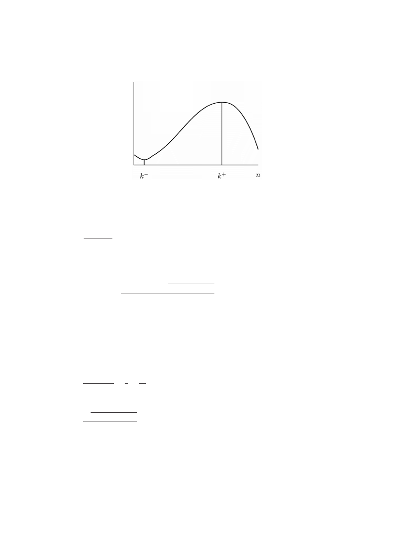
Fig. 1. Sketch showing the presumedshape of the distribution.
To determine when the ratio is =; ¿ ; or ¡ 1, we solve for k in the equation
kr(n − k)
(k + 1)c
= 1
⇔ rnk − rk
2
= ck + c
⇔ rk
2
+ (c − rn)k + c = 0
⇔ k
±
=
−(c − rn) ±
(c − rn)
2
− 4rc
2r
:
(6)
The ratio is greater than one for values of k in the interval between the two solutions,
so the probabilities P
k
are nondecreasing from k
−
to k
+
. The probabilities decrease
for k ¡ k
−
and k ¿ k
+
. Thus, the mode is either 0 or k
+
. By choosing the
reintroduction rate parameter suTciently large, the probability of being in state zero
can be made as small as desired, so in this case the mode is k
+
. Note that k
±
are
independent of the reintroduction rate a.
Considering the terms that make up k
±
, we note that
−(c − rn)
2r
=
n
2
−
c
2r
;
is somewhat less than half the population size, while
(c − rn)
2
− 4rc
2r
is slightly less than the 0rst term. Thus, the interval of increasing probabilities covers
nearly the entire range of population sizes, if r and c are 0xed, in which case the
mode is near n, the population size. If c grows linearly with n, then the mode can
be signi0cantly less than n (see Fig.
), which means the infection becomes endemic,
with a stable proportion of the population infected.
J.C. Wierman, D.J. Marchette / Computational Statistics & Data Analysis 45 (2004) 3–23
9
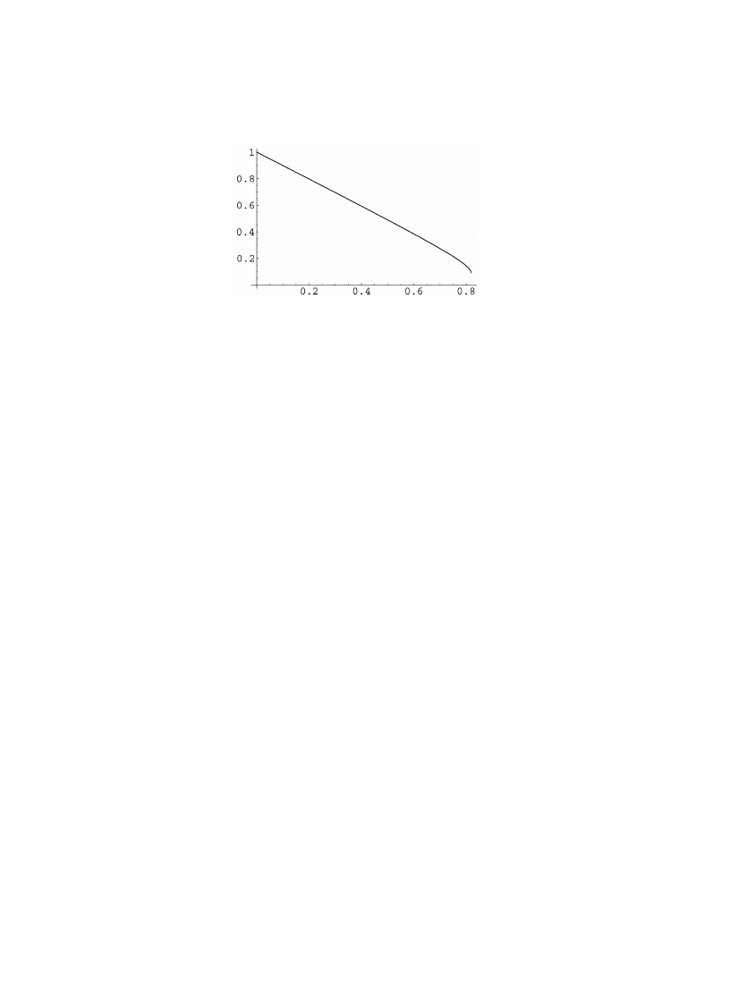
Fig. 2. The mode calculated using Eq. (
) with r = 0:01 and n = 100 as a function of c. The proportion of
infectedmachines is plottedon the y-axis.
As can be seen in Fig.
, the mode of the number of infected machines is roughly
linear in the cure rate, for 0xed r and n.
3.2. Probability distribution approximations
As seen in Eq. (
), the stationary distribution of the birth-and-death process modeling
the number of infected computers depends on the cure and infection rates only through
their ratio c=r. (This is intuitively clear because c and r are both rates in the Markov
process setting, andrescaling time wouldnot change the stationary distribution.) Since c
is the cure rate per individual while r is the infection rate from each infected individual,
it is appropriate to consider c=r as a function of n to achieve a balance between the
total infection andtotal cure rates for the population. In this section, we will discuss
three approximations for the stationary distribution, which are valid in four diJerent
ranges of c=r. While we sketch the ideas of the proofs here, the details will be deferred
to an Appendix.
3.2.1. Small c=r (Poisson approximation)
If the cure rate is suTciently small relative to the infection rate, intuitively one
wouldexpect nearly all the population to be infectedmost of the time. This suggests
that a Poisson distribution, often used to model occurrences of rare events, may be
appropriate for the number of uninfectedcomputers. The following result makes this
precise.
Let X
n
and Y
n
= n − X
n
denote the number of infectedanduninfectedcomputers
respectively, when the process is in the invariant distribution {P
i;n
: i = 0; 1; : : : ; n}.
(We use the subscript n to indicate the possible dependence upon the population
size n.)
Lemma 1. If lim
n→∞
c=r = b ¿ 0, then lim
n→∞
P[Y
n
= i] = (b
i
e
−b
=i!) ∀i = 0; 1; 2; : : : ,
i.e. Y
n
asymptotically has a Poisson(b) distribution.

10
J.C. Wierman, D.J. Marchette / Computational Statistics & Data Analysis 45 (2004) 3–23
Proof (Sketch). Denoting the distribution of Y
n
by {Q
i;n
: i = 0; 1; : : : ; n}, we have
Q
i;n
= P
n−i;n
=
1
Z
n
a
c
1
n − i
r
c
n−i−1
(n − i)!
i!
for i = 0; 1; : : : ; n, with Q
n;n
= P
0;n
= 1=Z
n
, where Z
n
is a normalizing factor. It is useful
to express the other Q
i;n
as multiples of Q
0;n
as
Q
i;n
=
n
n − i
c
r
i
1
i!
Q
0;n
;
(7)
where Q
0;n
now plays the role of a normalizing factor. Without the factor n=(n − i)
we wouldhave Q
0;n
= e
−c=r
exactly, giving us the Poisson(c=r) distribution. Since
n=(n − i) → 1 as n → ∞ for each 0xed i = 0; 1; : : :, and c=r → b, it suTces to show
that Q
0;n
→ e
−b
. This is accomplishedin the Appendix, using a geometric series to
boundthe tail probability andthus the normalizing factor.
The approximation by a Poisson distribution leads to the interpretation that it is a
rare event that a particular computer is not infected, when c and r are 0xed. This
wouldcorrespondto a particularly virulent disease, anddoes not correspondwell to
observations of computer virus infections, in which a small proportion of the population
is infectedat a given time.
Given the Poisson approximation result when c and r are constant, it is clear that we
must consider cases where c and r, or at least the ratio c=r, depends on the population
size n, to achieve a suitable balance between infection andcuring processes. This is
intuitive if one recalls that the cure rate c is per individual, while the total infection
rate per individual is a multiple of r.
Remark: For completeness, we note that if c=r → 0 as n → ∞, a simpler anal-
ysis than above shows that the probability that all computers are infectedconverges
to one.
3.2.2. Moderate c=r (Normal approximation)
To achieve a better balance between the cure rate andtotal infection rate, we con-
sider the case where
n
= c=r → ∞ as n → ∞. The parameter b appearedas the mean
of the approximating Poisson distribution in the case where c=r was asymptotically
constant. Since the Poisson distribution becomes asymptotically Normal as the mean
converges to in0nity, it is natural to expect that the number of uninfectedcomputers
among n total computers, denoted here by Y
n
, has an approximate Normal distribution
for some rates of
n
= c=r → ∞. The following proof is basedon converting the Pois-
son approximation into a Normal approximation, under the condition that c=r = o(n)
as n → ∞.
Lemma 2. If
n
= o(n), then lim
n→∞
P[a ¡ (Y
n
−
n
)=
√
n
¡ b] = (b) − (a) for
all −∞ ¡ a ¡ b ¡ ∞, where denotes the standard Normal cumulative distribution
function.

J.C. Wierman, D.J. Marchette / Computational Statistics & Data Analysis 45 (2004) 3–23
11
Proof (Sketch). For convenience, we denote the frequency function of the Poisson(
n
=
c=r) distribution by {
i;n
: i = 0; 1; 2; : : :}. We may then calculate
P
a ¡
Y
n
−
n
√
n
¡ b
= P[
n
+ a
n
¡ Y
n
¡
n
+ b
n
]
=
n
+b
√
n
i=
n
+a
√
n
Q
i;n
=
n
+b
√
n
i=
n
+a
√
n
n
n − i
c
r
i
1
i!
Q
0;n
:
Under our hypothesis, however, Q
0;n
→ 0, but we can again boundthe sum of proba-
bilities to show that
e
c=r
Q
0;n
= 1 + o(1):
Thus, we have
P
a ¡
Y
n
−
n
√
n
¡ b
= (1 + o(1))
n
+b
√
n
i=
n
+a
√
n
n
n − i
i;n
:
Since
n
+ b
√
n
= o(n), then 1 6 n=(n − i) 6 1 + o(1) for all i 6
n
+ b
√
n
, so
P
a ¡
Y
n
−
n
√
n
¡ b
= (1 + o(1))
n
+b
√
n
i=
n
+a
√
n
i;n
:
However, as n → ∞, the Poisson(
n
= c=r) distribution, normalized, is asymptotically
Normal, so
n
+b
√
n
i=
n
+a
√
n
i;n
→ P [a ¡ W ¡ b];
where W has a standard Normal distribution.
This result shows that the number of infectedcomputers is approximately Normal
with mean n − c=r andvariance c=r, when c=r → ∞, c=r = o(n). However, in this case,
we still have the proportion of the population that is infected, (n − c=r)=n, converging
to 1.
3.2.3. Large c=r (Normal and logarithmic limit)
We now consider the case when the cure rate increases roughly linearly with the
population size. From the analysis of the mode, we see that typically a stable propor-
tion of the population will be infected. In this situation, with approximately n infected
computers, 0 ¡ ¡ 1, the population cure rate is approximately cn, while the popu-
lation infection rate is approximately r(1 − )n. Stability can be achievedwhen these
are balanced.

12
J.C. Wierman, D.J. Marchette / Computational Statistics & Data Analysis 45 (2004) 3–23
We consider c=r = nd + o(n) as n → ∞, and0ndthat the distribution has quite
diJerent behavior when d ¡ 1 than when d ¿ 1.
Lemma 3. If
n
= nd + o(n); d ¡ 1, then lim
n→∞
P[a ¡ (Y
n
−
n
)=
√
n
¡ b] =
(b) − (a):
Proof (Sketch). As in the proofs of Lemmas
and
, we consider the number of
uninfectedcomputers, viewing its distribution as closely relatedto the Poisson(
n
)
distribution
Q
i;n
=
n
n − i
i;n
K
n
;
where K
n
normalizes the sum to produce a probability distribution. For d ¡ 1, we can
choose ! ¿ 0 such that ! ¡ d and d + ! ¡ 1, anduse ChernoJ bounds to show that
P
|Y
n
− nd| ¿ !n
6 e
−"n
for some " ¿ 0. Thus, nearly all the probability is concentratednear nd, where the
factor n=(n − i) is near 1=(1 − d). This can be usedto establish that the normalizing
constant is approximately 1 − d, so
P
a ¡
Y
n
−
n
√
n
¡ b
= (1 + o(1))
n
+b
√
n
i=
n
+a
√
n
i;n
→ (b) − (a)
as
n
→ ∞ as in the proof of Lemma
Lemma 4. If
n
= nd + o(n); d ¿ 1, then
lim
n→∞
P[X
n
= k] =
a=kd
k−1
1 − log(1 − 1=d)
;
k = 0; 1; : : : :
Proof (Sketch). Note that
P
k;n
=
a
k
r
c
k−1
(n − 1)!
(n − k)!
1
3
F
1
({1; 1; n − 1}; {2}; −r=c)
:
Under our hypothesis,
r
c
k−1
(n − 1)!
(n − k)!
→
1
d
k−1
:
Note that
3
F
1
({1; 1; n − 1}; {2}; −r=c) is a normalizing factor which is independent
of k. Since the series of limiting probabilities converges in k geometrically, lim
n→∞
3
F
1
({1; 1; n − 1}; {2}; −r=c) is the normalizing constant for the limiting distribution,
which can be computedby standardseries convergence methods from calculus.
This limiting distribution diJers from the logarithmic distribution,
P[X = k] =
#
k
−k log(1 − #)
k = 1; 2; : : : ;
where 0 ¡ # ¡ 1, due to the atom at zero (and necessary renormalization). The log-
arithmic distribution is discussed in
, Chapter 7. It arises in a

J.C. Wierman, D.J. Marchette / Computational Statistics & Data Analysis 45 (2004) 3–23
13
model strongly related to ours, being the steady-state distribution of a birth and death
process with rates
i
= i, i 6 1, and
i
= i, i ¿ 1, but
1
= 0, a process appearing
in
in the context of animal group dynamics. We are not aware of these
distributions arising in previous analyses of computer virus epidemic models.
4. Simulation
The National Computer Security Association reports a computer virus infection rate
of approximately 35 infections per 1000 computers per month. See the web page at
www.webmastersecurity.com/ncsa97virusprevalencesurveya.htm
for the 1997 report. The ICSA computer virus prevalence report, available at
www.trusecure.com/html/tspub/pdf/vps20001.pdf
reports slightly diJerent, but similar, rates (see Table
). The Sophos computer virus
lab
www.sophos.com/virusinfo/whitepapers/prevention.html
reports that in the secondquarter of 2000, approximately 800 new viruses were in-
troduced each month, with over 50,000 known viruses in existence. Telcordia Tech-
nologies (
) reports the number of machines on the Internet to be 127
million as of October 2001. Other sources of statistics on virus prevalence are available
at
http://www.securitystats.com/virusstats.asp
and
These reports, along with information on the propagation methods of known viruses,
allow one to produce ballpark estimates for n, r and a. One then wouldbe interested
in studying the properties of the system as a function of c. Numbers are available
for various of these parameters for diJerent intervals, allowing some determination of
trends and rates of change.
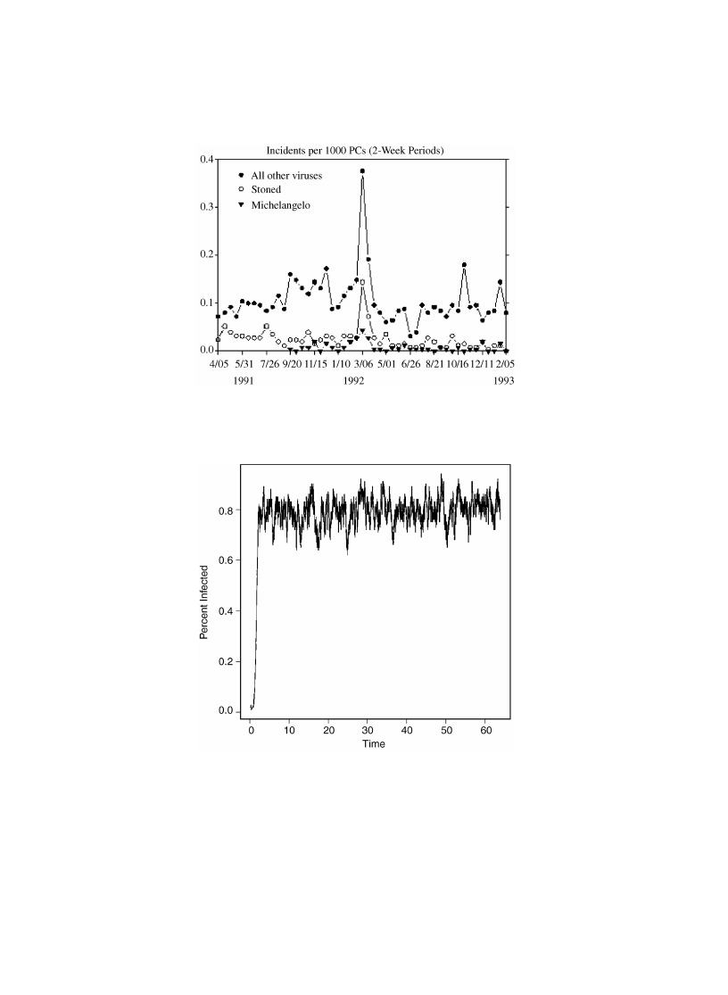
report some virus prevalence data from 1991 which shows
a relatively low level of virus infections (see Fig.
). It shouldbe notedthat the spike
in the middle is interpreted to be the result of a higher level of vigilance and reporting,
as opposedto an actual increase in the number of viruses.
Some simulations can illustrate the model. In order to simulate this process, we take
a two step approach. First, we draw a random time, t ∼ exp(r + c), corresponding
to the time until the next event. Then we Vip a (biased) coin to determine if the
event was an infection or a cure: we draw a uniform random variable y andtest if
y ¡ R
n;m
=(R
n;m
+C
m
) (infection) or y ¿ R
n;m
=(R
n;m
+C
m
) (cure), where R
n;m
=r(n−m)m
and C
m
= cm. In the event that m = 0, we set m to 1 at time t ∼ exp a later.
Table 1
Rate of infection per 1000 computers in the 0rst two months of each year
Year
Rate of infection
1996
10
1997
21
1998
32
1999
80
2000
91
14
J.C. Wierman, D.J. Marchette / Computational Statistics & Data Analysis 45 (2004) 3–23
Fig. 3. Number of virus incidents reportedper 1000 PCs for two speci0c viruses, Stoned(open circles) and
Michelangelo (triangles), and all other viruses (closed circles) during two week periods ending with the
indicated date. From
, with permission (? 1993 IEEE).
Fig. 4. A simulation run with parameters a = 1, r = 0:05, c = 1 and n = 100.
Set a = 1, r = 0:05, c = 1 and n = 100. In this case, Eq. (
) gives an estimate for
the mode of 79.75 infected computers. Note that since k is an integer, this says that
the mode falls at 80 for these parameters. Fig.
shows the time progression of the
simulation. For these parameters Mathematica gives a value of P
0
= 7 × 10
−34
, while
J.C. Wierman, D.J. Marchette / Computational Statistics & Data Analysis 45 (2004) 3–23
15
60
70
80
90
100
0.00
0.02
0.04
0.06
0.08
N = 8597 Bandwidth = 1.476
Density
+
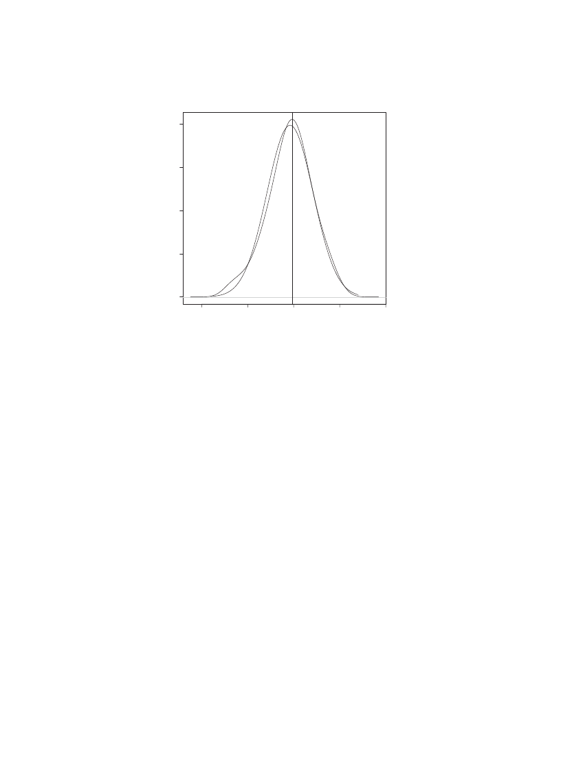
Fig. 5. A kernel estimator 0t to the 0nal 8536 observations of the simulation depicted in Fig.
. The estimate
for the mode given in Eq. (
) is depicted by a solid line, with the mode of the kernel estimator indicated
by a dotted line. A Normal density with parameters equal to the sample mean and standard deviation for
these data is depicted as a dotted curve. A “+” is drawn at the mode of the Normal density.
Eq. (
) gives a value of 1:7 × 10
−34
. Thus the approximation agrees to an order of
magnitude with the “exact” value provided by Mathematica (note that even in this
“exact” calculation, the transcendental functions must be approximated numerically).
Note that from a practical standpoint, these values indicate that the time to extinction
for these values of the parameters is so large as to be of no practical consequence.
In order to estimate the mode of the limiting distribution, we consider the time steps
from t = 10 on. A kernel estimator is 0t to these data and plotted in Fig.
. The mode
of the kernel estimator is at 79.20, in agreement with the analysis.
Solving Eq. (
) for a maximum, using Mathematica’s numerical optimization solver,
results in a value of 80.25, in agreement with the above analysis (remembering that
Mathematica is treating the function as a continuous one, while in reality it is discrete).
The mean andvariance of the distribution are also available, either in closedform
using Mathematica or numerically. For the parameters of the simulation we obtain a
mean 79.75 (comparedto the simulation value of 79.20) anda variance of 20.322
(comparedto the simulation value of 25.213). Thus the theory is in close agreement
with the simulation.
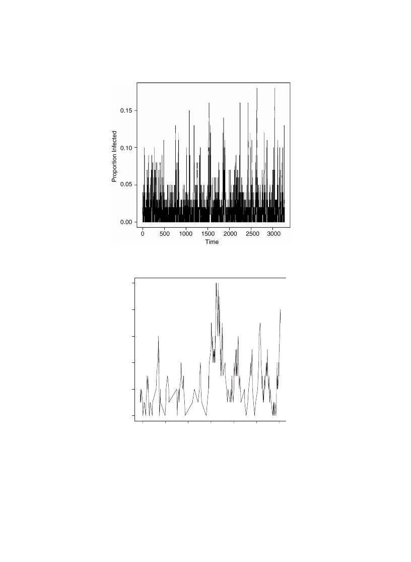
To illustrate the large c behavior, Figs.
show the results of a simulation with
a=1; r=0:008 and c=1. This shows the tendency of the epidemic to die out with large
c. The reintroduction rate is relatively large as well, causing the infection to start up
again quickly after an extinction. Note that as many as 15% of the computers become
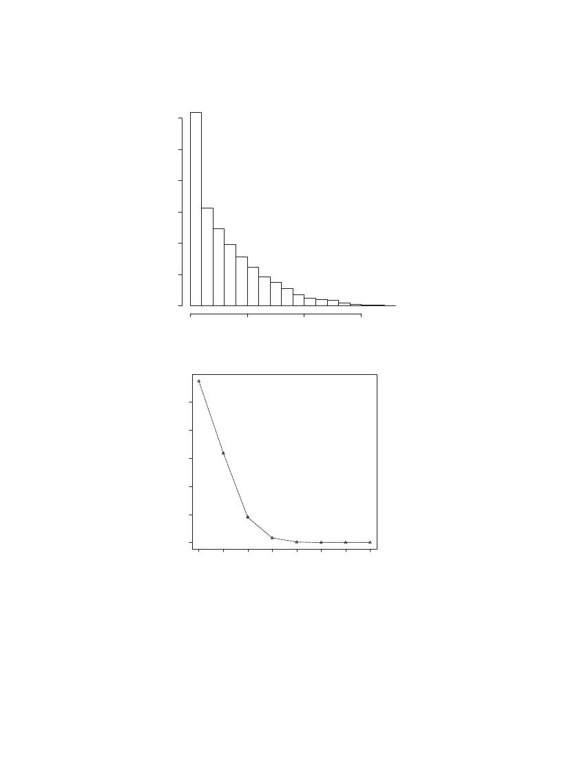
infectedwith these rates. Fig.
shows the logarithmic distribution for the number of
infectedmachines.
16
J.C. Wierman, D.J. Marchette / Computational Statistics & Data Analysis 45 (2004) 3–23
Fig. 6. A similar simulation to that in Fig.
with a = 1; c = 1; r = 0:008 and n = 100.
240
250
260
270
280
290
300
0.00
0.02
0.04
0.06
0.08
0.10
Time
Proportion Infected
Fig. 7. A subset of the simulation of Fig.
For small c behavior, Figs.
and
show close agreement between the theoretical
andsimulation values for Q
i;n
of Eq. (
). This demonstrates the closeness of the Poisson
approximation even for moderate values of n.
J.C. Wierman, D.J. Marchette / Computational Statistics & Data Analysis 45 (2004) 3–23
17
Number of Infected Machines
Density
0
5
10
15
0.00
0.05
0.10
0.15
0.20
0.25
0.30
Fig. 8. A histogram of the number of infectedmachines parameters c = 1; r = 0:008; a = 1 and n = 100.
0
1
2
3
4
5
6
7
Number Uninfected Machines
Probability
0.5
0.4
0.3
0.2
0.1
0.0
Fig. 9. Q
i;1000
for a = 30, c = 0:01 and r = 0:018. The theoretical values from Eq. (
) are depicted as a solid
curve, with the simulation values depicted as a dotted curve. The curves essentially overlap in this 0gure.
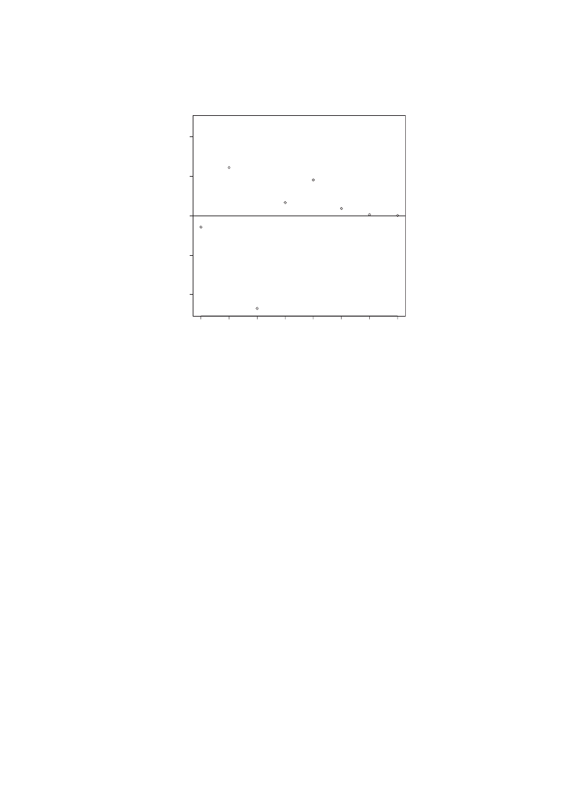
5. Discussion
We proposed an epidemic model for the prevalence of computer viruses in a ho-
mogeneous closedpopulation of computers. We determinedthe invariant distribution
18
J.C. Wierman, D.J. Marchette / Computational Statistics & Data Analysis 45 (2004) 3–23
0
1
2
3
4
5
6
7
-0.002
-0.001
0.000
0.001
0.002
Number Uninfected Machines
P
Theory
P
Simulation
−
Fig. 10. The diJerence between the theoretical Q
i;1000
(Eq. (
)) andsimulation values, from the simulation
of Fig.
. As in that simulation, a = 0:03, c = 0:001 and r = 0:01.
of the number of infectedcomputers, andfoundapproximations to this distribution
for diJerent ranges of parameters of the model. A key feature of the model is the
existence of a thresholdvalue of c=r at which a dramatic change occurs in the distri-
bution, from approximately logarithmic (which has a 0nite mean regardless of popula-
tion size) to asymptotically normal (when properly standardized), corresponding to the
mean increasing without boundas the population size increases. The thresholdmay be
expressedas c=r = n. This implies that the ratio of cure rate to infection rate must be
much larger to prevent a widespread infection in a large population than in a small
population.
Due to the homogeneity assumedin the model, it is more applicable to local networks
or clusters of computers, where reintroduction may correspond to infection by a virus
from outside the local network. A model where the population increases in time might
be more appropriate for the entire Internet.
A more realistic model might have diJerent levels of subgroups of computers, which
communicate among themselves at diJerent rates. For example, a three level model
might consist of departments within a company, companies, and the entire Internet.
DiJerent computers (or groups of computers, such as those with speci0c operating
systems), might have diJerent probabilities of becoming infected when exposed. Pre-
ventative action (“vaccination” or the installation of anti-virus software) couldbe taken
into account. In the literature on epidemics, each of these eJects has been considered
in some model, but not all combined in any model for which rigorous mathematical
analysis has been done.

J.C. Wierman, D.J. Marchette / Computational Statistics & Data Analysis 45 (2004) 3–23
19
Acknowledgements
Professor Wierman gratefully acknowledges research support through the Navy-
American Society for Engineering Education sabbatical program and the Acheson J.
Duncan Fundfor the Advancement of Research in Statistics. Dr. Marchette was sup-
portedthrough the Naval Surface Warfare Center Seeds program.
Appendix
Proofs. To 0nish the proof of Lemma
we needto 0ll in the details of the Poisson
convergence. To prove that Q converges to a Poisson distribution, however, we must
show that the Q
i;n
do not all converge to zero as n → ∞ because they contain the
normalizing factor Z
n
.
Choose I
n
¿ c=r suTciently large that I
n
! ¿ n. Then we may boundthe tail proba-
bility by a geometric series to obtain
n−1
i=I
n
Q
i;n
6
c
rI
n
I
n
1
1 − (c=nI
n
)
n
I
n
!
Q
0;n
(1 + o(1)):
Note also that Q
n;n
=Q
0;n
→ 0: Thus,
Q
0;n
I
n
i=0
c
r
i
1
i!
6 1 =
n
i=0
Q
i;n
6 Q
0;n
n
n − I
n
I
n
i=0
c
r
i
1
i!
+ o(1)
6 Q
0;n
n
n − I
n
e
c=r
+ o(1)
:
Since I
n
! ¿ n requires that I
n
→ ∞, andwe may choose I
n
to be o(n), asymptotically
we have
e
b−!
lim sup
n→∞
Q
0;n
6 e
c=r
lim sup
n→∞
Q
0;n
6 1 6 e
c=r
lim inf
n→∞
Q
0;n
6 e
b+!
lim inf
n→∞
Q
0;n
for each ! ¿ 0, so lim
n→∞
Q
0;n
exists andis equal to e
−b
. This implies that lim
n→∞
Q
i;n
exists andis equal to
b
i
1
i!
e
−b
for i = 1; 2; : : : :

20
J.C. Wierman, D.J. Marchette / Computational Statistics & Data Analysis 45 (2004) 3–23
To complete the proof of Lemma
, we now verify our assumption, Q
o;n
=e
−c=r
=
1 + o(1). First, note that
1 =
n
i=0
Q
i;n
¿ Q
0;n
n−1
i=0
c
r
i
1
i!
;
so
Q
o;n
6
1
n−1
i=0
(c=r)
i 1
i!
=
1
e
c=r
−
∞
i=n
(c=r)
i
1=i!
6
1
e
c=r
−
(c=r)
n
n!
e
c=r
=
e
−c=r
1 −
(c=r)
n
n!
:
By Stirling’s Formula
(c=r)
n
n!
≈
(c=r)
n
√
2n
n+ 12
e
−n
=
1
√
2
ce
r
n
n
−n− 12
= O(n
− 12
);
if ce=r ¡ n, or, equivalently c=r 6 n=e. Then
Q
0;n
e
−c=r
6
1
1 − B=
√
n
6 1 +
A
√
n
;
(8)
for some A; B ¿ 0.
For a boundin the other direction
1 =
n
i=0
Q
i;n
=
I
n
i=0
(c=r)
i
1
i!
Q
0;n
+
n−1
i=I
n
+1
Q
i;n
+ Q
n;n
(9)
for some I
n
¿ c=r. For I
n
= o(n),
I
n
i=0
c
r
i
1
i!
Q
0;n
6
n
n − I
n
Q
0;n
I
n
i=0
c
r
i
1
i!
= (1 + o(1))Q
0;n
∞
i=0
c
r
i
1
i!
= (1 + o(1))Q
0;n
e
c=r
:

J.C. Wierman, D.J. Marchette / Computational Statistics & Data Analysis 45 (2004) 3–23
21
For the secondterm in Eq. (
n−1
i=I
n
+1
Q
i;n
=
n−1
i=I
n
+1
n
n − 1
c
r
i
1
i!
Q
0;n
:
Note that for i ¿ I
n
¿ c=r, the factor (c=r)
i
=i! is decreasing.
As before, use Stirling’s Formula
(c=r)
I
n
I
n
!
≈
(c=r)
I
n
√
2I
I
n
+ 12
n
e
−I
n
=
1
√
2
ce
r
I
n
I
−I
n
− 12
n
:
Choose I
n
≈ 2e(c=r), so c=r ≈ (1=2e)I
n
, then
(c=r)
I
n
I
n
!
≈
1
√
2
1
2
I
n
I
n
I
I
n
− 12
n
6
D
2
I
n
:
Then
n−1
i=I
n
+1
Q
i;n
= Q
0;n
n−1
i=I
n
+1
n
n − 1
c
r
i
1
i!
6 Q
0;n
(n − I
n
)
n
D
2
I
n
6 Q
0;n
Dn
2
2
−2e(c=r)
6 Q
0;n
Ee
−2(c=r)
:
From Eq. (
), we have
P
0
= Q
n;n
= o(e
−c=r
):
Combining, we have
1 6 (1 + o(1))Q
0;n
e
c=r
+ Q
0;n
Ee
−2c=r
+ o(e
−c=r
)
6 (1 + o(1))Q
0;n
e
c=r
;
so, from this andEq. (
1 − o(1) 6
Q
0;n
e
−c=r
6 1 +
A
√
n
:
Thus we obtain asymptotic normality when c=r → ∞ and c=r = o(n).
For Lemma
, we needto compute the normalizing constant. To evaluate this nor-
malizing constant, we write the probabilities (ad=r)(1=k)(r=d)
k
as (ad=r)(1=k)x
k
using
x = r=d, andsum (1=k)x
k
as follows. Notice that for |x| ¡ 1,
∞
k=1
1
k
x
k
=
∞
k=1
x
k−1
=
1
1 − x
= (−log(1 − x))
:

22
J.C. Wierman, D.J. Marchette / Computational Statistics & Data Analysis 45 (2004) 3–23
So,
∞
k=1
1
k
x
k
= −log(1 − x) + C
andevaluating at x = 0 shows that C = 1. Thus
lim
n→∞
(c + aF
n
) =
ad
r
1 − log
1 −
r
d
if r ¡ d, and
lim
n→∞
P
k
=
(1=k)(
r
d
)
k
1 − log(1 − r=d)
:
The mean infectedpopulation size in the limiting distribution is
∞
k=1
(r=d)
k−1
1 − log(1 − r=d)
=
1
(1 − r=d)(1 − log(1 − r=d))
=
d
(d − r)(1 − log(1 − r=d))
;
(10)
which is 0nite for r ¡ d. Similarly, all moments are 0nite when r ¡ d. However, for
r ¿ d, the mean infectedpopulation size tends to in0nity as n → ∞.
References
Abreu, E.M., 2001. Computer virus costs reach $10.7b this year. The Washington Post, Sept 1, 2001.
available at
http://www.washtech.com/news/netarch/12267-1.html
Ball, F., 1983a. The threshold behavior of epidemic models. J. Appl. Probab. 20, 227–241.
Ball, F., 1983b. A threshold theorem for the Reed-Frost chain-binomial epidemic. J. Appl. Probab. 20,
153–157.
Ball, F., 1999. Stochastic and deterministic models for SIS epidemics among a population partitioned into
households. Math. Biosci. 156, 41–67.
Ball, F., Donnelly, P., 1995. Strong approximations for epidemic models. Stoch. Proc. Appl. 55, 1–21.
Bartholomew, D.J., 1976. Continuous time diJusion models with random duration of interest. J. Math.
Sociology 4, 187–199.
Caraco, T., 1979. Ecological response of animal group size frequencies. International Co-operative Publishing
House, Fairland, MD, pp. 371–386.
Cavender, J.A., 1978. Qausi-stationary distributions of birth-and-death processes. Adv. Appl. Probab. 10, 570
–586.
Darroch, J.N., Seneta, E., 1967. On quasi-stationary distributions in absorbing continuous-time 0nite markov
chains. J. Appl. Probab. 4, 192–196.
Jacquez, J.A., Simon, C.P., 1993. The stochastic SI model with recruitment and deaths. I. comparison with
the closedSIS model. Math. Biosci. 117, 77–125.
Johnson, N.L., Katz, S., Kemp, A.W., 1992. Univariate Discrete Distributions. Wiley, New York.
Kendall, D.G., 1956. Deterministic and stochastic epidemics in closed populations. In: J. Neyman (Ed.),
ThirdBerkeley Symposium on Mathematical Statistics andProbability, Vol. 4. University of California
Press, California, pp. 149–165.
Kephart, J.O., White, S.R., 1991. Directed–graph epidemiological models of computer viruses. In: 1991 IEEE
Computer Society Symposium on Research in Security andPrivacy, Oakland, California, pp. 343–359.
Kephart, J.O., White, S.R., 1993. Measuring andmodeling computer virus prevalence. In: 1993 IEEE
Computer Society Symposium on Research in Security andPrivacy, Oakland, California, pp. 2–15.

J.C. Wierman, D.J. Marchette / Computational Statistics & Data Analysis 45 (2004) 3–23
23
Kephart, J.O., White, S.R., Chess, D.M., 1993. Computers andepidemiology. IEEE Spectrum 30, 20–26.
Kryscio, R.J., LefFevre, C., 1989. On the extinction of the SIS stochastic logistic epidemic. J. Appl. Probab.
27, 685–694.
Martin-LNof, A., 1986. Symmetric sampling procedures, general epidemic processes, and their threshold limit
theorems. J. Appl. Probab. 23, 265–282.
Murray, W., 1988. The application of epidemiology to computer viruses. Comput. Security 7, 139–150.
NHasell, I., 1996. The quasi-stationary distribution of the closed endemic SIS model. Adv. Appl. Probab. 28,
895–932.
NHasell, I., 1999. On the time to extinction in recurrent epidemics. J. R. Statist. Soc. B 61, 309–330.
Oppenheim, I., Shuler, K.E., Weiss, G.H., 1977. Stochastic theory of nonlinear rate processes with multiple
stationary states. Physica A 88, 191–214.
Ross, R., 1915. Some a Priori Pathometric Equations. Br. Med. J. 1, 546.
Ross, S., 1996. Stochastic Processes. Wiley, New York.
Scalia-Tomba, G., 1985. Asymptotic 0nal size distribution for some chain-binomial processes. Adv. Appl.
Probab. 17, 477–495.
von Bahr, B., Martin-LNof, A., 1980. Threshold limit theorems for some epidemic processes. Adv. Appl.
Probab. 12, 319–349.
Weiss, G.H., Dishon, M., 1971. On the asymptotic behavior of the stochastic and deterministic models of
an epidemic. Math. Biosci. 11, 261–265.
Wolfram, S., 1996. The Mathematica Book, 3rd Edition. Cambridge University Press, New York.
Document Outline
- Modeling computer virus prevalence with a susceptible-infected-susceptible model with reintroduction
Wyszukiwarka
Podobne podstrony:
System Dynamic Model for Computer Virus Prevalance
Is Your Cat Infected with a Computer Virus
Some human dimensions of computer virus creation and infection
The dynamics of computer virus infection
A framework for modelling trojans and computer virus infection
How To Think Like A Computer Scientist Learning With Python
An Undetectable Computer Virus
Data security from malicious attack Computer Virus
Computer Virus Propagation Model Based on Variable Propagation Rate
Improving virus protection with an efficient secure architecture with memory encryption, integrity a
Prosecuting Computer Virus Authors The Need for an Adequate and Immediate International Solution
Formal Affordance based Models of Computer Virus Reproduction
Classification of Packed Executables for Accurate Computer Virus Detection
Threats to Digitization Computer Virus
The Virtual Artaud Computer Virus as Performance Art
Zero hour, Real time Computer Virus Defense through Collaborative Filtering
Computer Virus Operation and New Directions
więcej podobnych podstron