Statistical testing of individual differences in sensory profiling

Per Bruun Brockhoff

*

Department of Mathematics and Physics, Royal Veterinary and Agricultural University, Thorvaldsensvej 40, DK-1871 Frederiksberg C, Denmark

Received 29 July 2002; received in revised form 21 November 2002; accepted 28 November 2002

Abstract

A generalization of the approach of Brockhoff and Skovgaard [Food Quality & Preference, 5 (1994), 215] is given. The emphasis

is on univariate assessor performance in sensory profiling. Statistical significance tests for difference between assessors of scaling,
variability and sensitivity will be given. A test for disagreement effect is also presented. In addition the approach will provide indi-
vidual scaling, variability, disagreement and sensitivity values, that can be used for subsequent tabulation, plotting and statistical
analysis. The method of maximum likelihood is used throughout and all computations are implemented in a SAS

1

Macro PAN-

MODEL that is available via the author’s homepage: http://www.dina.kvl.dk/ per.
#

2003 Elsevier Science Ltd. All rights reserved.

Keywords:

Analysis of variance; Assessor performance; Individual differences; Maximum likelihood analysis; Multipicative interaction; SAS macro;

Sensory profile data; Statistical testing

1. Introduction

The investigation of individual differences in sensory

profiling has been the topic of several papers over the
years, see, for example,

Lundahl and McDaniel (1990,

1991), Naes and Solheim(1991), and Brockhoff and
Skovgaard (1994)

. The present paper is a continuation

of the latter with two main novel contributions: (1)
Providing a statistical significance test for sensitivity
differences. (2) Presenting the entire approach as a
practical tool for the analysis of individual differences in
a full sensory profile data set supported by a publically
available SAS

1

macro. A conceptual difference between

the presented approach and other approaches is that
formal statistical models are specified and formal max-
imum likelihood theory is used. Although earlier meth-
ods also provided significance tests for certain effects we
give here a more comprehensive collection of formally
performed likelihood ratio tests.

Consider an over-simplified sensory experiment with

no session effects. Assume also that we have a simple
oneway sample structure, that is, the samples represent
only one single ‘treatment factor’. Let Y

asr

denote the

r

th replicate of a sensory score given by assessor a for

sample s, where r=1,. . .,R, a=1,. . .,A and s=1,. . ., S.
The standard ANOVA model with sample and assessor
main effects together with the sampleassessor interac-
tion effect may be written as

Y

asr

¼

a

þ

s

þ

as

þ

"

asr

;

"

asr

N

0;

2

and

independent

ð

1Þ

The application of this model has the purpose to get

information about the samples (

s

) but accounting

properly for possible assessor differences. For this we
would typically assume that

a

and

as

are random

variables leading to a so-called mixed model ANOVA.
Viewpoints on how to performan ANOVA properly in
the sensory context are given in the papers

Steinsholt

(1998), Naes and Langsrud (1998)

and discussion

papers, for example,

Brockhoff (1998b)

. This is not the

issue of the present approach. Instead the focus is on the
individual differences.

Fig. 1

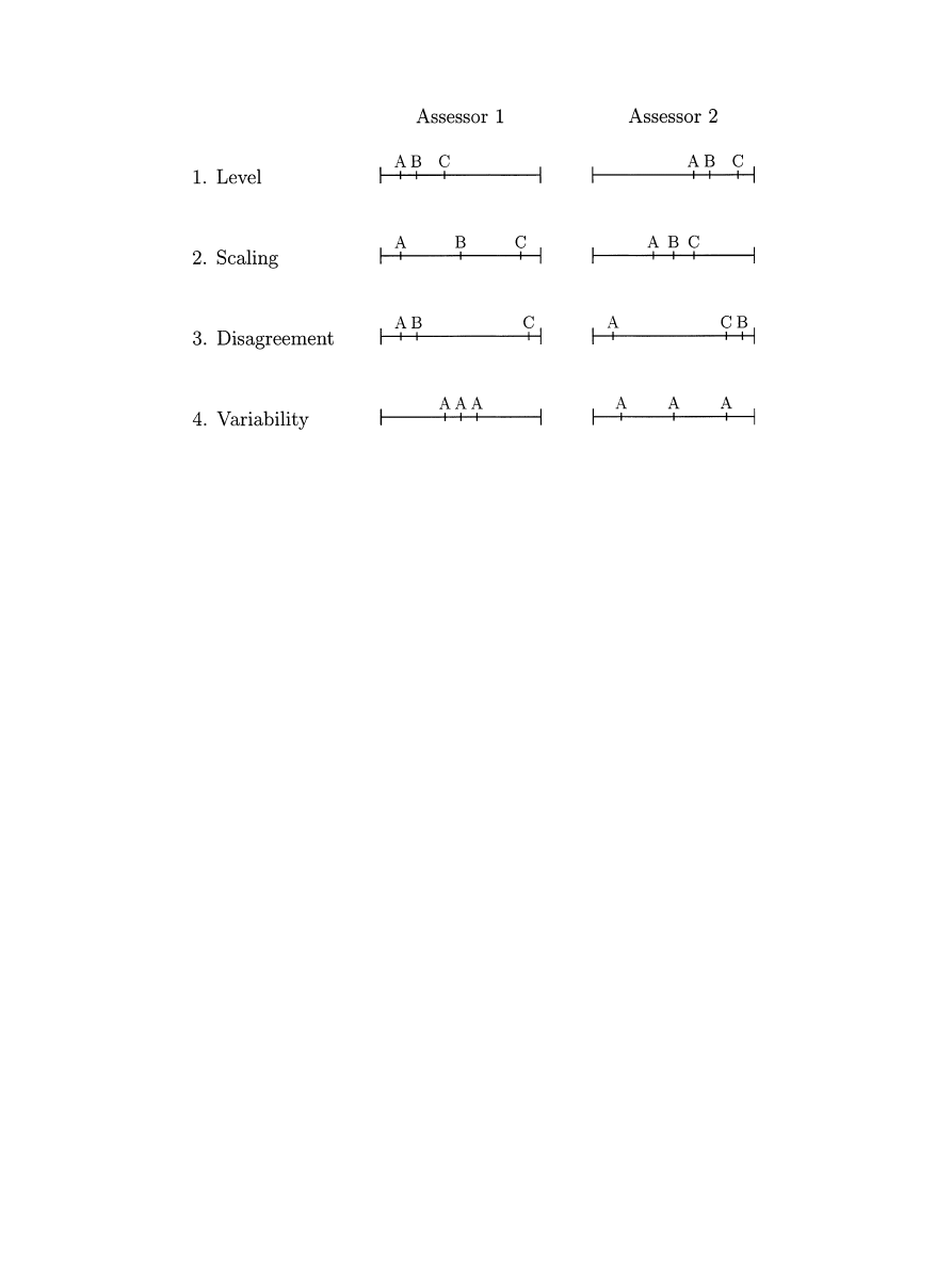
illustrates what differences

we may encounter on a univariate scale. Together, scal-
ing differences and disagreements constitute the asses-
sorsample interaction. The disagreement part of the
interaction is, apart fromthe exact inverse ranking,
what

Stone and Sidel (1985)

refers to as ‘cross-over’

interaction. And the scaling part corresponds to ‘mag-
nitude interaction’ in the terminology of

Stone and Sidel

(1985)

.

0950-3293/03/$ - see front matter # 2003 Elsevier Science Ltd. All rights reserved.
doi:10.1016/S0950-3293(03)00007-7

Food Quality and Preference 14 (2003) 425–434

www.elsevier.com/locate/foodqual

* Tel.: [phone]; fax: [phone].

E-mail address:

[e-mail] (P.B. Brockhoff).

We start out with a discussion of how the acknowl-

edgement of the possible differences illustrated in

Fig. 1

leads to the so-called basic assessor model. Next, the
generalized assessor model is presented. This is the key
model for the entire approach. The following two sec-
tions will then more precisely state which significance
tests we performand which individual values we com-
pute. A short section gives the principles of the under-
lying computations without going into details and
finally an example is given showing the features of this
approach using the available SAS

1

macro PANMO-

DEL. Some technical details are given in the

Appendix

.

2. The basic assessor model

The standard ANOVA model given by

(1)

accounts

for differences of type 1, 2 and 3, cf.

Fig. 1

. The assessor

level differences are the main effects (

a

). Scaling as well

as disagreement differences will come up as interaction
effects (

as

). Variability differences are not accounted

for in

(1)

: one of the standard assumptions behind usual

ANOVA is variance homogeneity. But it is easy to spe-
cify ‘the same’ model allowing for different assessor
variabilities:

Y

asr

¼

a

þ

s

þ

as

þ

"

asr

;

"

asr

N

0;

2

a

0

and

independent

ð

2Þ

So this model takes all four listed assessor differences
into account and will indeed serve as a basic ‘reference’
model for the approach of the paper.

Note that the only difference between

(1) and (2)

is

the subscript on the error variance

a

0

2

. This means that

a comparison of how well each of the two models fits

the data will lead to a statistical significance test for the
hypothesis of equal variances (‘variability homo-
geneity’). Following this maximum likelihood principle
of testing for effects we can achieve a test for disagree-
ment: we must specify a model including every type of
assessor differences except for the disagreement. This is
the basic assessor model as given a thorough treatment
in

Brockhoff and Skovgaard (1994)

:

Y

asr

¼

a

þ

a

s

þ

"

asr

;

"

asr

N

0;

2

a

and

independent

ð

3Þ

To explain how this model comes up, let us take the

reference model

(2)

as starting point and argue step by

step how to construct a model including assessor differ-
ences type 1, 2 and 4 and not type 3, cf.

Fig. 1

. Inclusion

of the

a

and

a

2

-parameters ensures that type 1 and type

4 are present. The

s

-parameters (sample main effects)

should also be there as we still want the model to
express sample differences. The only thing not reused
from

(2)

at this point is the interaction term

as

. First

note again that the assessorsample interaction effect
may be seen as a sum of scaling effects and non-linear
(non-scaling) effects:

Interaction ¼ Scaling þ Disagreement

Instead of the general interaction term

as

we must spe-

cify a termthat expresses scaling effects only. The dif-
ferences in scaling can be expressed by specifying
individual scaling constants ~

a

. Interpreting the sample

main effects

s

in

(2)

as true sample values of the sensory

property in question (on some common scale) the scal-
ing effect is then the product ~

a

s

. This should then be

substituted for

as

in

(2)

leading to

Fig. 1. The four basic assessor differences for a single sensory attribute. By disagreement we mean all interaction effect not attributable to scaling
differences. As indicated this will include ranking differences (apart fromthe exact inverse ranking that will come up as a scaling effect).

426

P.B. Brockhoff / Food Quality and Preference 14 (2003) 425–434

Y

asr

¼

a

þ

s

þ

~

a

s

þ

"

asr

¼

a

þ

1 þ ~

a

s

þ

"

asr

Renaming

a

¼

1 þ ~

a

, we obtain the basic assessor

model

(3)

. This shows that although at first sight, the

sample main effects seem to be missing in the assessor
model, they are indeed present as a part of the scaling
effect.

The sensitivity is defined as the squared ‘signal-to-

noise’ ratio:

Sensitivity

a

¼

2
a

=

2

a

Comparing data fits for model

(3)

with model

(2)

gives a test for disagreements. In fact, this comparison
amounts to a comparison of the estimated individual
variances in the two models: ^

2
a

0

and ^

2
a

. The former is

the actual within sample variation for each individual
whereas the latter also include the disagreement effects
(if any). We can thus by a comparison on individual
level obtain individual measures of disagreements as:

Disagreement

a

¼

ffiffiffiffiffiffiffiffiffiffiffiffiffiffiffiffiffi

2

a

2

a

0

q

:

Using the assessor model as reference model we will be
able to test for scaling effects by fitting a restricted ver-
sion with no scaling effects. We will also be able to test
for sensitivity differences using a similar approach. And
finally, applying the assessor model for each sensory
attribute will provide estimates for individual scalings,
variabilities, disagreements and sensitivities for each
attribute. These can be used to investigate by summary
statistics and/or plotting the individual differences in
further detail. We return to the interpretation of the
individual parameters in

Section 5

. In the basic assessor

model there is a simple one-way sample structure. In the
following it will be clear that it all generalizes to arbi-
trary complex sample structures without changing the
setup for testing and estimating individual differences.

3. The general assessor model

In most realistic situations, the experimental design

structure will have a complexity such that the basic
assessor model will be too simplistic. The complex
structure may include crossed and nested sample treat-
ment effects, order and carry-over effects, session and
blocking effects, etc. As indicated in

Brockhoff and

Skovgaard (1994)

it is possible to extend the basic

assessor model in such a way that one may include an
arbitrary complex structure while maintaining the
assessor part with individual differences in level, scaling
and variability in the model. In short, the generalization
is carried out by substituting for

s

in

(3)

the sumof all

effects in play. In our context in which information
about the assessor differences is the target, it means that
we can acknowledge the true structure of the data, and
still do all the testing outlined earlier.

For a precise definition of the generalized assessor

model we would have to introduce a notation for the
general linear model. Instead we illustrate how it works
for the example given in the present paper. We assume
now, more realistically, that the replications were car-
ried out in several sessions, and we want to account for
the replication main effects. Replication may here
represent a single session, if all samples are tested in
each session, or a ‘collection’ of sessions in time. The
general assessor model now becomes

Y

asr

¼

a

þ

a

s

þ

r

ð

Þ þ

"

asr

;

"

asr

N

0;

2

a

and

independent:

ð

3aÞ

This is then a model that allows for multiplicative
interaction between assessors and everything else, but
only through the same individual scaling constants. This
goes together with the following thinking: no matter
what goes on that might change the perception of the
samples, this will eventually ‘go through’ each indivi-
dual’s use of the scale before becoming an actual
observed sensory score. Fromthe point of view of the
present paper this generality does not change anything
regarding the target information: statistical significance
tests for individual differences together with individual
estimates for scaling, variability, disagreement and sen-
sitivity.

The general version of the reference model

(2)

may

now be written as

Y

asr

¼

a

þ

s

þ

r

þ

as

þ

ar

þ

"

asr

;

"

asr

N

0;

2

a

0

and

independent

ð

2aÞ

when, in the following, we refer to

(2a) and (3a)

we

think of these as the general definitions of the models.
These general models are really specified by a specifica-
tion of all effects one would include in an ANOVA
model except for all effects related to assessors, we call
these the sample structure effects.

4. Statistical significance tests

We will performsignificance tests for the following

four assessor effects:

(I) Variability differences (4. in

Fig. 1

)

(II) Presence of disagreements (3 in

Fig. 1

)

(III) Scaling differences (2. in

Fig. 1

)

(IV) Sensitivity differences

P.B. Brockhoff / Food Quality and Preference 14 (2003) 425–434

427

More formally this corresponds to the testing of the

following hypotheses:

H

(I)

:

2

1

¼ ¼

2

A

(versus

(2a)

)

H

(II)

: Model

(3a)

holds true (versus

(2a)

)

H

(III)

:

1

¼ ¼

A

(versus

(3a)

)

H

(IV)

:

2

1

2

1

¼ ¼

2

A

2

A

(versus

(3a)

)

The test in

(I)

is carried out as a Bartlett corrected w

2

-

test as in

Brockhoff and Skovgaard (1994).

1

The more

general sample structure does not give any difficulties
for the Bartlett test. The tests in

(II), (III) and (IV)

are

based on the maximum likelihood method, in which two
nested models are compared by the likelihood ratio sta-
tistic. We use here approximate F-test statistics as
described in

Brockhoff (1998a)

.

The test for equal sensitivities in

(IV)

is new in this

context. In

Brockhoff and Skovgaard (1994)

it was

shown that the quantities

a

2

/

a

2

are measures of indivi-

dual sensitivities that relate closely to F-test statistics
fromindividually performed ANOVAs. This, however,
is only true if in fact there are no disagreements. We
also see that the tests in

(III) and (IV)

are carried out

‘versus

(3a)

’. Froma strictly statistical point of view this

means that we assume that the assessor model

(3a)

holds truly, and under that assumption we test the scal-
ing and sensitivity differences. However, if disagreement
is present the tests still make sense, but the interpreta-
tion of scaling (and consequently of sensitivity) changes:
it has now a ‘consensus’ interpretation. If an individual
does not agree with the panel as a whole he/she will get
lower scaling and sensitivity values. To understand this,
one may take a look at the basic assessor model

(3)

. The

scalings appear as individual regression coefficients in
regressions on the common (‘consensus’) values of the
samples

s

. If an individual ranks entirely different than

the consensus he/she may very well obtain an individual
regression coefficient of zero although he/she uses all of
the scale. And as the sensitivities are direct functions of
the scalings the same interpretation applies: an individual
may be a good ‘discriminator’ as measured by the indivi-
dual F-test statistic, but if his/her ranks of discrimination
do not agree with the panel as a whole, he/she will not be
called ‘sensitive’ in the sense of the present paper.

5. Individual parameters

In addition to the four significance tests an important

source of information are the estimated individual

parameters. We let now p, p=1,. . .,P, be a numbering of
the sensory attributes. We have then as an output from
the macro individual scalings, variabilities (standard
deviations), disagreements and (‘signed’) sensitivities for
each combination of assessor and attribute:

Scalings :

^

ap

Standard deviations :

^

a

0;p

Disagreements :

ffiffiffiffiffiffiffiffiffiffiffiffiffiffiffiffiffiffiffiffiffiffi

^

2

ap

2

a

0;p

q

Signed sensitivities :

^

ap

=^

ap

The ‘signed’ sensitivities will have the same sign as the
scaling factor. Note that the standard deviations are the
real individual variability measures, that is, the individually
sized residuals fromthe reference model

(2a)

. These figures

summarize what goes on in the panel with respect to scal-
ing, variability, disagreement and sensitivity. The inter-
pretations should be combined with the outcomes of the
significance tests. Two different aims emerge at this point:

Within panel comparisons of the assessors.

Between panel comparisons, when several panels
evaluated the same kind of samples.

And the possible tools for this may be categorized as:

1. Tabulation.
2. Plotting.
3. Further statistical analysis.

It is beyond the scope of this paper to cover all six

combinations of aims and tools. A few tables and plots
for the within panel comparisons of the assessors are
given. For each of the four effects an assessor-by-attri-
bute table is presented. If the effect is significant for an
attribute the values for the two most extreme assessors
are given. Biplots of the full matrix of individual values
are used subsequently.

6. Computations

In order to obtain the tests of the previous section we

must be able to maximize the likelihood for each of the
four models:

1. Model

(2a)

2. Model

(3a)

3. Model

(3a)

with the additional restriction that

1

¼ ¼

A

.

4. Model

(3a)

with the additional restriction that

2
1

=

2

1

¼ ¼

2
A

=

2

A

.

For 1, 2 and 3 this was derived for the basic assessor

model in

Brockhoff and Skovgaard (1994)

and this can

1

The formula for the Bartlett test in

Brockhoff and Skovgaard

(1994)

has a misprint: The symbols R and P must be interchanged.

428

P.B. Brockhoff / Food Quality and Preference 14 (2003) 425–434

be generalized directly to the more general setting of the
present paper. The model

(2a)

is simply fitted by fitting

for each assessor the model given by the sample struc-
ture effects. The general assessor model

(3a)

is fitted by

a type of alternating least squares algorithmalternating
between individual regressions (for ‘known’ values of
the sample structure effects) and weighted ANOVAs
(for ‘known’ values of the individual parameters

a

,

a

and

a

). The model

(3a)

with the homogeneous scaling

restriction

1

= =

A

is fitted by a simplified version

of the alternating algorithmjust outlined. In this case
the algorithmcorresponds to an iterative weighted least
squares procedure. The derivation of an algorithmfor
the model

(3a)

with the homogeneous sensitivity

restriction

2
1

=

2

1

¼ ¼

2
A

=

2

A

requires a little con-

sideration, but follows along the same lines. Details are
given in the

Appendix

.

All computations presented in the paper are imple-

mented as the SAS

1

macro PANMODEL that is avail-

able

through

the

author’s

homepage:

http://

www.dina.kvl.dk/ per. The later example will illustrate
what the macro provides and what it can do. No exact
SAS

1

syntax will be given as this may be subject to

change over time. The macro is self-explanatory.

7. Example

We consider here data froma study on frozen peas,

see

Bech, Hansen, and Wienberg (1997)

. Sixteen pea

samples were profiled by a panel of 11 assessors. They
were evaluated in three replicates using 14 descriptors
measured by a continuous line scale from 0 to 15. We
applied the PANMODEL macro with the sample main
effects on 16 levels and the replication main effect on
three levels as the sample structure effects, cf.

(2a) and

(3a)

. The current version of the macro PANMODEL

takes as input a SAS

1

data set with the entire sensory

data as it would be prepared to performregular analysis
of variances for each attribute. The output fromPAN-
MODEL is three plain text-files (ASCII):

1. A log-file with results of data checks, iteration

convergence

information

and

detailed

sig-

nificance test results.

2. A result file with summary tables of the sig-

nificance tests and extreme individuals.

3. A data file with the estimated individual standard

deviations, disagreements, scalings and sensitiv-
ities for each assessor and attribute.

The data check is an automated procedure that

checks whether there are some ‘singularities’ in the data
that make it impossible to carry out the analyses. And if
this is the case the ‘singularities’ are removed and the
removal registered in the log-file. For instance, it will

take out an assessor for a given attribute, if the assessor
has exactly the same score (possibly missing) for all
observations on that attribute. It makes no sense to
look for a scaling and variability value for such an
assessor. This data check makes the macro robust
against programbreak downs for ‘m

essy’ data set

(imbalance, lots of missing values, low information
data, too many specified attributes, etc.).

The current version of the PANMODEL macro pro-

vides first of all a table corresponding to

Table 1

. In

Table 1

the main significance results are presented. We

see that for all attributes except for mealiness and juici-
ness there is a significant difference (on 5% level) in the
assessor’s variability. Whenever not specified we use the
5% test level. There are only significant disagreement
problems in few cases, but the assessors do indeed use
the scale differently for almost all attributes (except for
pea odour). And perhaps the most interesting of them
all: for all attributes except for pea taste the assessors
have different sensitivities. The assessors did vary (sig-
nificantly) in their variability on pea taste and they also
differed in the scaling, but apparently these two effects
cancel each other out such that the sensitivites are not
significantly different. For mealiness and juiciness, for
which the variabilities were homogeneous, the differ-
ences in scaling imply differences in the sensitivity.

Next the PANMODEL macro gives for each of the

four features tables of the most extreme individuals. In

Table 2

we see the least and the most reproducible

assessor for each attribute when in fact significant dif-
ferences exist. These standard deviations should be
interpreted in light of the line scale [0,15]. A standard
deviation of 2.10 for pea odour assed by assessor 6
expresses that the average deviation fromhis/her aver-
age value for replications of identical samples is 2.10 for
assessor 6. Using the standard normal population

Table 1
Summary of statistical tests of individual differences

Attribute

Variability

Disagreement

Scaling

Sensitivity

Pea odour

***

***

Pod odour

**

**

***

Sweet odour

***

**

***

Earthy odour

***

***

***

Pea taste

***

**

*

Pod taste

**

*

***

***

Sweet taste

*

*

*

*

Bitterness

***

***

**

Earthy taste

***

*

***

***

Crispiness

***

**

***

***

Juiciness

***

***

Hardness

***

***

***

Mealiness

***

***

Skin viscosity

**

**

***

* 5% significance.
** 1% significance.
*** 0.1% significance.

P.B. Brockhoff / Food Quality and Preference 14 (2003) 425–434

429

interpretation, this means that his/her distribution (at
least

approximately

95%

of

it)

will

span

22.10=4.20 on each side of the average value. A

span of more than 8 is large on a [0,15] line scale. In
general the smallest standard deviation seems to be
clearly below 1 corresponding to a span between 2 and
4. Overall, assessor 1 and in particular assessor 6 seem
to be the least reproducible, whereas assessor 8 and
assessor 11 are the most reproducible.

Turning to

Table 3

we see the similar presentation of

the disagreement results. There were only significant
disagreements for five attributes and individual values
are hence only given for these attributes. The inter-
pretation of the disagreement values differs in principle
fromthe other three values. A significant disagreement
effect means that the disagreements overall are different
fromzero, and not necessarily different fromassessor to
assessor. For pod odour the most agreeing individual
was assessor 1, and assessor 2 was the most disagreeing.
The sizes of these disagreement effects can be inter-
preted as ‘disagreement induced standard deviations’ on
the [0,15] line scale. For further insight in the kind of
disagreement present for a given attribute further plot-
ting or tabulation is necessary. A plot like Fig. 3 in

Brockhoff and Skovgaard (1994)

would illustrate the

individual contributions to the disagreement. We will
not pursue this further here.

In

Table 4

the most extreme scalings are presented.

Recall that these in general have a ‘consensus’ inter-
pretation, cf.

Section 4

. The interpretation of the scaling

sizes depends on how we parametrize the asssessor
model. As pointed out in the Appendix, the PANMO-
DEL macro standardizes the sample structure values,
such that they have a standard deviation of 1. One may
roughly think of the sample structure values lying
between 2 and 2. A scaling of, say, 2 then means that
this individual uses from 4 to 4 on each side of his/hers
average value. Again this is on the [0,15] sensory scale.
Using the outlined standardization enables direct scal-
ing comparisons across attributes.

Finally in

Table 5

we see the signed sensitivities. Small

values indicate low sensitivity and large values indicate
high sensitivity. As discussed in

Section 4

they also have

‘consensus’ interpretations, in the sense that a disagree-
ing assessor will tend to be non-sensitive although he/
she may have a high individual F-test statistic. The size
of the sensitivities are mainly to be used in a relative
manner, although since we know the size interpretations
of both numerator and denominator this could be
transformed into a direct interpretation of the sensitiv-
ity. In practice, however, this approach seems not very
informative. Rather one can say that an individual with
a sensitivity of 2 is twice as sensitive as an individual
with a sensitivity of 1. And since the scalings are directly
comparable across attributes, the same goes for the
sensitivities.

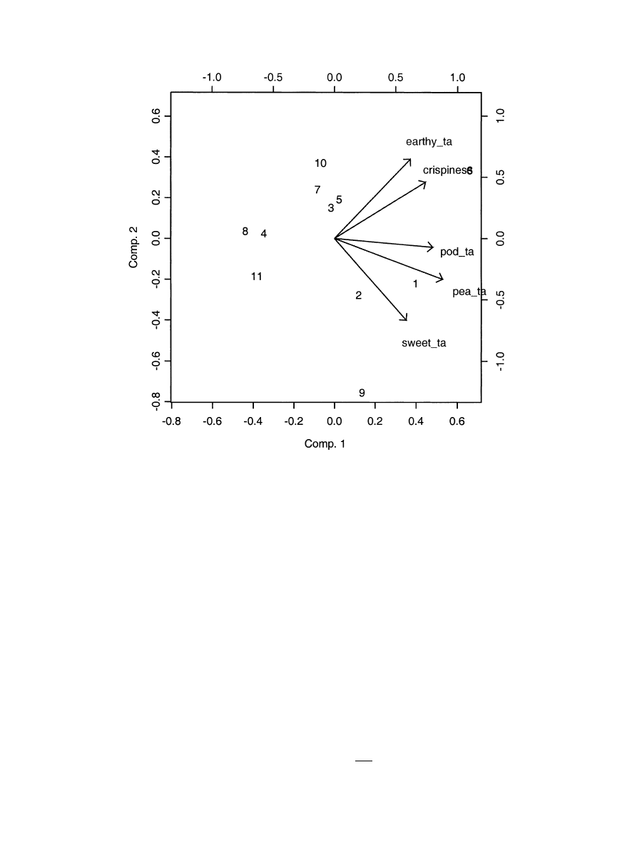
Finally, the macro provides for each of the four fea-

tures an AQ matrix of numbers, where Q is the num-
ber of attributes. The use of biplots as a visualization
tool is an obvious idea. In

Figs. 2 and 3

biplots of the

sensitivities and the disagreement contributions are
shown using only the attributes for which statistical
significances were seen. It is seen that assessors 1, 9, 7
and 8 are the most extreme wrt. discrimination: assessor
9 is particularly sensitive to crispiness and juiciness,

Table 2
The smallest and largest individual standard deviations ^

a

0;p

for the

attributes exhibiting significant variability differences

Attribute

1

2

3 4

5

6

7

8

9

10

11

Pea odour

2.10

0.68

Pod odour

2.01 0.83

Sweet odour

1.93 0.76

Earthy odour

2.13

0.45

Pea taste

1.63

0.72

Pod taste

2.01

0.83

Sweet taste

1.98

0.87

Bitterness

0.81

2.04

Earthy taste

1.26

0.30

Crispiness

2.22

0.60

Hardness

2.04

0.71

Skin viscosity

0.79

1.49

Table 3
The smallest and largest individual disagreement contributions

ffiffiffiffiffiffiffiffiffiffiffiffiffiffiffiffiffiffiffiffiffiffi

^

2

ap

^

2

a

0;p

q

for the attributes exhibiting significant disagreement

Attribute

1

2

3

4

5

6

7

8

9

10

11

Pea taste

0.61

1.69

Pod taste

1.78

0.76

Sweet taste

0.81

2.06

Earthy taste

0.40

1.94

Crispiness

2.02

0.70

Table 4
The smallest and largest individual scalings ^

ap

for the attributes

exhibiting significant scaling differences

Attribute

1

2

3

4

5

6

7

8

9

10 11

Pod odour

0.21

2.90

Sweet odour

0.11

1.83

Earthy odour

0.37 2.04

Pea taste

1.97

0.80

Pod taste

0.56

1.99

Sweet taste

0.76

2.88

Bitterness

3.04

1.06

Earthy taste

0.11

2.19

Crispiness

0.35

3.65

Juiciness

3.72

0.92

Hardness

2.62

0.38

Mealiness

3.90

1.51

Skin viscosity 2.50

1.12

430

P.B. Brockhoff / Food Quality and Preference 14 (2003) 425–434

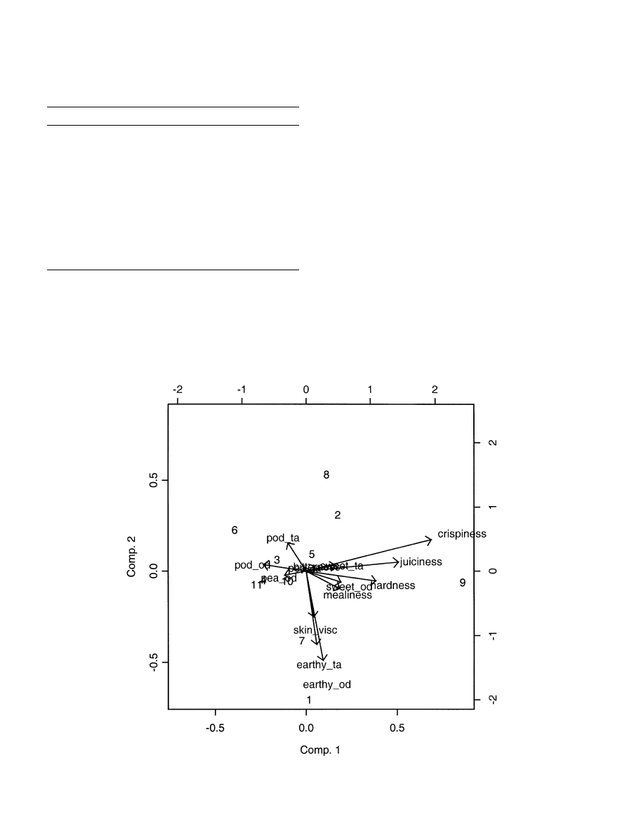
whereas assessor 1 and 7 are particularly sensitive to
earthy taste/odour, whith assessor 8 being particularly
insensitive in that respect. Assessors 4, 6, 8, 9 and 11 are
the most extreme wrt. disagreement: assessors 6 and 9 is
the mostly disagreeing persons overall, assessor 4, 8 and
11 are the mostly agreeing persons in the panel.

8. Discussion

A parametric model based approach based on repe-

ated use of maximum likelihood methods was presented
as a tool to investigate individual differences in sensory
profile data. A common objection to the maximum
likelihood approach is the complexity and the need for
complex iterative procedures that may fail to converge
in realistic situations. This is overcome by the publically
available SAS

1

macro PANMODEL, in which the

model specification is exactly like most SAS

1

proce-

dures. And the used iterative procedures are robust
alternating algorithms based on regular SAS

1

proce-

dures such that missing values, etc. is handled auto-
matically. Anyway, the user does not in general have to
worry about these iterations.

But, of course, the entire mystery of the world is not

solved in this paper. As was pointed out in

Section 5

we

only addressed a minor part of the possible combina-
tions of aims and tools: tabulation and plotting of
within panel comparisons of assessors. For between
panel comparisons it will be more relevant to study the
assessor-to-assessor

distributions

of the

individual

effects, as for instance in

Brockhoff (1998a)

, where a

Table 5
The smallest and largest individual sensitivities ^

ap

=^

ap

for the attri-

butes exhibiting significant sensitivity differences

Attribute

1

2

3

4

5

6

7

8

9

10

11

Pea odour

0.13

0.81

Pod odour

0.10

1.74

Sweet odour

0.10

1.12

Earthy odour 2.00

0.11

Pod taste

0.29

1.58

Sweet taste

1.53 0.37

Bitterness

1.89 0.58

Earthy taste 1.69 0.17
Crispiness

0.16

3.14

Juiciness

0.52

2.79

Hardness

2.21

0.26

Mealiness

2.26

0.91

Skin viscosity 2.02

0.59

Fig. 2. Biplot of sensitivities.

P.B. Brockhoff / Food Quality and Preference 14 (2003) 425–434

431

subsequent ANOVA was performed on individual
parameter values. An important example of subsequent
statistical analysis would be to performformal tests as
the basis of the

Tables 2–5

instead of just showing the

two most extremes. This has number one priority for
improvement of the approach and the macro. Sub-
sequent tests like that could also be used to distinguish
in more detail between the different types of assessors.
As mentioned we do not address individual differences
in the multivariate structure.

As given here the approach is ready to be used for

panel

training

purposes,

panel

performance

doc-

umentation and as a sensory research tool. But we do
not address, as mentioned in

Section 1

, how/if this

should imply anything for the analysis of sample differ-
ences for which usually some kind of mixed model is
employed. In

Smith, Cullis, Brockhoff, and Thompson

(in press)

an analysis based on mixed multiplicative

models is suggested.This approach can be seen as a
combination of the heterogeneous scaling and varia-
bility approach having the assessors in focus, with a
mixed model approach having the samples in focus. A
comparison of results for the pea data example is also

given in that paper. More sensometric research is
needed to investigate the possible implications of such
an approach on the sensory tradition of analysis of
variance.

Acknowledgements

The research was partly supported by the Danish

FØTEK 2 Programme.The author is grateful to Pascal
Schlich, INRA, Dijon, France for a number of helpful
comments improving the presentation considerably.

Appendix. Algorithm for model

(3a)

with homogeneous

sensitivities

The hypothesis of homogeneous sensitivities

2
1

=

2

1

¼

¼

2
A

=

2

A

¼

c

can equivalently be expressed as

a

¼

a

c

;

c >

0;

a ¼

1; . . . ; A

For the basic assessor model this means that

Fig. 3. Biplot of disagreements.

432

P.B. Brockhoff / Food Quality and Preference 14 (2003) 425–434

Y

asr

¼

a

þ

s

a

þ

"

asr

;

"

asr

N

0;

2
a

=c

2

and

independent

or equivalently using a more compact notation

Y

asr

N

a

þ

a

a

;

2
a

=c

2

ð

4Þ

Assume we know the individual parameters

a

and

a

.

We can then rewrite

(4)

as

Y

asr

a

a

N

s

;

1=c

2

This is a standard ANOVA model for the transformed
observations and we can thus find estimates for c and

s

.

For known c and

s

the basic assessor model may be

rewritten

cY

asr

N c

a

þ

c

s

ð

Þ

a

;

2
a

that is, we need for each assessor to ‘solve’ a univariate
linear regression model with the additional restriction
that the variance must be the square of the slope:

X

i

N þ t

i

;

2

;

i ¼

1; . . . ; n

ð

5Þ

Minus twice the log-likelihood for this model is

2Log-likelihood ;

ð

Þ ¼

n

log

2

þ

1

2

X

n

i¼

1

x

i

t

i

ð

Þ

2

Differentiating and solving the equations to maximize
this function with respect to and gives

^ ¼

SP

tx

ffiffiffiffiffiffiffiffiffiffiffiffiffiffiffiffiffiffiffiffiffiffiffiffiffiffiffiffi

SP

2

tx

þ

4nSS

x

p

2n

ð

6Þ

^ ¼ x" ^t"

ð

7Þ

where

x" ¼

1
n

X

n

i¼

1

x

i

; x" ¼

1
n

X

n

i¼

1

x

i

; SP

tx

¼

X

n

i¼

1

x

i

x"

ð

Þ

t

i

t"

;

SS

x

¼

X

n

i¼

1

x

i

x"

ð

Þ

2

It is now easy to check by insertion in a given case

which one of the two possible -values gives the highest
likelihood.

So the algorithmfor the general assessor m

odel

M

1

with

the

homogeneous

sensitivity

restriction

becomes (we let N denote the total number of non-
missing observations for the sensory attribute in ques-
tion):

1. Make starting values for the

a

- and

a

-parameters

(fromthe fit of the general assessor model).

2. Make an ANOVA on the transformed observa-

tions with a model given by the sample struc-
ture effects, yielding c^ and ‘predicted’ values of
the sample structure effects for each single
observation in the data set. Denote these ^

i

,

i

=1,. . .,N.

3. Standardize the n

i

-parameters according to:

P

N

i¼

1

i

¼

0;

1

N

X

N

i¼

1

2
i

¼

1

4. Find individual parameters ^

a

and ^

a

accord-

ing to

(6) and (7)

applied for each assessor

using as x

i

the sensory score for the assessor

in question multiplied by c^ and as t

i

¼

c^

^

i

where the ^

i

is the predicted value of the

sample structure effect for the observation for
the assessor in question.

5. Repeat 2–4 until convergence.

The standardization over all observations in 3. is

slightly different than the standardization used in

Brockhoff and Skovgaard (1994)

: there we standardize

only over the different sample parameters. Such an
approach would not be feasible for complex sample
structures. The more general standardization above is
used throughout in this paper and in the SAS

1

Macro

PANMODEL. The choice of standardization does not
affect the test statistics, but does affect the estimates of
scaling. So to compare results across experiments one
must make sure that the same standardization is used,
for instance by applying the macro PANMODEL in all
analyses.

References

Bech, A. C., Hansen, M., & Wienberg, L. (1997). Application of house

of quality in translation of consumer needs into sensory attributes
measurable by descriptive sensory analysis. Food Quality and Pref-
erence

, 8, 329–348.

Brockhoff, P. M. (1998a). Assessor modelling. Food Quality and Pref-

erence

, 9, 87–89.

Brockhoff, P. B. (1998b). Discussion contribution. Food Quality and

Preference

, 9, 160–162.

Brockhoff, P. M., & Skovgaard, I. M. (1994). Modelling individual

differences between assessors in sensory evaluations. Food Quality
and Preference

, 5, 215–224.

Lundahl, D. S., & McDaniel, M. R. (1990). Use of contrasts for the

evaluation of panel inconsistency. Journal of Sensory Studies, 5,
265–277.

P.B. Brockhoff / Food Quality and Preference 14 (2003) 425–434

433

Lundahl, D. S., & McDaniel, M. R. (1991). Influence of panel incon-

sistency on the outcome of sensory evaluations from descriptive
panels. Journal of Sensory Studies, 6, 145–157.

Naes, T., & Solheim, R. (1991). Detection and interpretation of var-

iation within and between assessors in sensory profiling. Journal of
Sensory Studies

, 6, 159–177.

Naes, T., & Langsrud, O. (1998). Fixed or randomassessors in sensory

profiling?. Food Quality and Preference, 9(3), 145–152.

Smith, A., Cullis, B., Brockhoff, P. B., & Thompson, R. Multiplicative

mixed models for the analysis of sensory evaluation data. Food
Quality and Preference

doi:10.1016/S0950-3293(03)00014–4.

Steinsholt, K. (1998). Are assessors levels of a split-plot factor in the

analysis of variance of sensory profile experiments? Food Quality
and Preference

, 9(3), 153–156.

Stone, H., & Sidel, J. (1985). Sensory evaluation practices. Orlando,

FL: Academic Press.

434

P.B. Brockhoff / Food Quality and Preference 14 (2003) 425–434