Emissions and Economic Analysis of Ground Source Heat Pumps in Wisconsin

ENERGY CENTER

OF WISCONSIN

report

report

report

report

report

report

report

report

report

report

report

report

report

report

report

report

report

report

report

report

report

report

report

report

report

report

energy

center

Research Report

201-1

Emissions and Economic Analysis

of Ground Source Heat Pumps in

Wisconsin

December 2000

Research Report

201-1

Emissions and Economic Analysis of Ground

Source Heat Pumps in Wisconsin

December 2000

Prepared by

Global Energy Options

4634 Bonner Lane

Madison, WI 53704-1327

608.244.6436

Oak Ridge National Laboratories

1000 Bethel Valley Rd.

Oak Ridge, TN 37831-6070

865.574.2015

Contact: George Penn

Global Energy Options

Prepared for

ENERGY CENTER

OF WISCONSIN

595 Science Drive

Madison, WI 53711-1076

Phone: 608.238.4601

Fax: 608.238.8733

Email: ecw@ecw.org

WWW

ECW

ORG

This report was prepared as an account of work sponsored by the Energy Center of Wisconsin (

ECW

). Neither

ECW

, participants in

ECW

, the organization(s) listed herein, nor any person on behalf of any of the

organizations mentioned herein:

(a) makes any warranty, expressed or implied, with respect to the use of any information, apparatus, method,

or process disclosed in this report or that such use may not infringe privately owned rights; or

(b) assumes any liability with respect to the use of, or damages resulting from the use of, any information,

apparatus, method, or process disclosed in this report.

Project Manager

Craig Schepp
Energy Center of Wisconsin

Acknowledgements

Thanks to Steve Carlson from CDH Energy Corporation and G. Hetherington, A. Hubbard, and E. Mosher from
the Wisconsin Department of Natural Resources.

This report is funded by the Wisconsin Department of Administration, Division of Energy and
Intergovernmental Relations, through the Wisconsin Energy Bureau under the terms and conditions of this
Agreement.

Table of Contents

Abstract ........................................................................................................................................... i

Report Summary...........................................................................................................................i i

Introduction....................................................................................................................................1

History.................................................................................................................................1
Approach .............................................................................................................................2
What We Hoped to Learn ....................................................................................................2
Key Findings........................................................................................................................3

Methods...........................................................................................................................................4

Scenarios...............................................................................................................................4
Energy Use Analysis............................................................................................................5
HVAC Equipment Types and Efficiencies..........................................................................6

Systems Modeled.......................................................................................................... 6
Estimated Average Efficiencies ........................................................................................ 7

Emissions Analysis..............................................................................................................7

Daytypes ..................................................................................................................... 9
Sensitivity Analysis .................................................................................................... 10

Customer Economics..........................................................................................................11

Results...........................................................................................................................................13

Emissions Results ..............................................................................................................13
Emissions Breakeven..........................................................................................................19
Economics Results .............................................................................................................19

Discussion.....................................................................................................................................25

Introduction........................................................................................................................25
Interpretation of Results....................................................................................................25

Emissions.................................................................................................................. 25
Breakeven Emissions ................................................................................................... 26
Economics ................................................................................................................. 27
Impactors................................................................................................................... 28

Conclusions........................................................................................................................30
Recommendations ..............................................................................................................30
Limitations and Future Research........................................................................................31

References ....................................................................................................................................32

Appendix A- Emissions Model Input Data..............................................................................A-1

Appendix B- Sample Emissions Results .................................................................................B-1

iii

Tables and Figures

Table 1

Emissions Results – Green Bay..............................................................................iv

Table 2

Energy & Economics Results – Green Bay..............................................................v

Table 3

Scenarios for Which Analyses Were Performed.......................................................4

Table 4

HDD and CDD Estimates........................................................................................5

Table 5

Estimated Average Efficiencies: Commercial Buildings ...........................................7

Table 6

Estimated Average Efficiencies: Residential Type Buildings...................................7

Table 7

Daytypes Used for Emissions Analysis..................................................................9

Table 8

Emissions Sensitivity Analysis..............................................................................10

Table 9

Rates Used for Economic Analysis........................................................................11

Table 10

Blended Rates.........................................................................................................12

Table 11

Large School Emissions Results (Natural Gas Heating).........................................13

Table 12

Small School Emissions Results (Natural Gas Heating).........................................14

Table 13

Office Emissions Results (Natural Gas Heating)...................................................14

Table 14

Commercial Development Emissions Results (Natural Gas Heating) ...................15

Table 15

Residential Emissions Results (Natural Gas Heating) ...........................................15

Table 16

Commercial Development Emissions Results (LP Gas Heating)...........................16

Table 17

Residential Emissions Results (LP Gas Heating)...................................................16

Table 18

Commercial Development Emissions Results (Fuel Oil Heating)..........................17

Table 19

Residential Emissions Results (Fuel Oil Heating)..................................................17

Table 20

Commercial Development Emissions Results (Electric Heating)...........................18

Table 21

Residential Emissions Results (Electric Heating)...................................................18

Table 22

Large School Energy and Economics Results.........................................................20

Table 23

Small School Energy and Economics Results.........................................................21

Table 24

Office Energy and Economics Results ...................................................................22

Table 25

Community Development Energy and Economics Results ...................................23

Table 26

Residential Energy and Economics Results............................................................24

Table A-1

Alliant (WP&L) Power Plant Characteristics ..................................................... A-2

Table A-2

Alliant (WP&L) Emissions Rate Data ................................................................ A-3

Table A-3

Daytype Definitions........................................................................................... A-4

Table A-4

Season Definitions............................................................................................... A-5

Table B-1

Emissions Analysis Sample Output Table: Large School, WPS, Green Bay.......B-1

Abstract

A result of the combined sponsorship of the Wisconsin Focus on Energy program, the Wisconsin
Geothermal Association, and the Energy Center of Wisconsin, the research underlying this report
has two main objectives. First, the research team investigated the impact on emissions resulting
from the application of ground source heat pumps (GSHP). Second, the team estimated the
resultant customer economics for application of this technology in new buildings being
constructed in Wisconsin.

We analyzed building energy use for each of the 8760 hours that make up the year. We then
compared this energy use to Wisconsin’s current operation of power plants that provide power
throughout Wisconsin to estimate impacts on several component emissions, assuming economic
dispatch. Finally, we estimated customer economic indicators related to installing GSHPs. Our
investigation included five building types in three different climate regimes, served by three
different utilities.

Based on the energy use of GSHP and conventional HVAC systems, we determined the potential
emissions reductions for each building type in each weather/utility area. For commercial buildings
our calculations indicate significant reductions in CO

emissions, as well as reductions in NO

and particulates in all but one scenario, while SO

emissions always increase. Finally, mercury

(Hg) emissions show less consistency; depending on the building type and weather regime, Hg
either slightly increases or slightly decreases. Conversely, all types of emissions primarily
increased from application of GSHP’s in the residential sector where natural or LP gas is
available. However, GSHPs installed in the residential sector where the home would otherwise be
heated with oil or electricity resulted in emissions reductions.

Finally, we analyzed the economics of this technology compared to conventional systems
appropriate for each building type, from the building owner’s perspective. We have found that
GSHPs can be an economically viable HVAC system for commercial buildings under certain
conditions. The economic viability in the residential sector appears more tenuous.

Our results suggest that designers of Wisconsin Public Benefits programs should consider this
technology in the future for commercial buildings in Wisconsin. For residential buildings Public
Benefits should consider promoting this technology where neither natural gas nor LP gas is
available. Wisconsin Public Benefits initiatives may also consider promotions in the residential
sector if needed to improve economies of scale in Wisconsin markets. In addition, the results also
suggest that electric utilities may want to examine this technology for inclusion in their future
commercial energy efficiency programs.

vii

Report Summary

Introduction

Precedent shows that Ground Source Heat Pumps (GSHP) provide superior HVAC performance
for many buildings, while offering improved efficiency and lower operating costs than
conventional HVAC systems. Further, the EPA has demonstrated significant reductions in most
emissions from the national deployment of this technology. This has led the EPA and DOE to
join forces in a variety of efforts to facilitate the increased application of GSHP technologies.

The Focus on Energy program, the Wisconsin Geothermal Association, and the Energy Center of
Wisconsin seek to learn how the economics and emissions benefits apply to the application of
this technology in new buildings built throughout Wisconsin. Global Energy Options was
retained to develop estimates of economics and emissions impacts for a variety of application
scenarios. Oak Ridge National Laboratory was also a major contributor and partner in this project
providing in-kind support to perform energy and economic analysis for several of the scenarios.

Methods

This report documents the environmental impacts of the technology, in the form of emissions
reductions. We also estimate the typical economic capabilities of this technology, from the
building operator’s perspective. Results outline fifteen scenarios, which are based on three
weather regimes, combined with matching utility generation:

•

Green Bay weather and Wisconsin Public Service

•

Madison weather with Alliant Energy, and

•

Eau Claire weather and Northern States Power

In addition, five “building types” were analyzed against these weather and utility combinations:

•

Large School

•

Small School

•

Office

•

Community Development, and

•

Residential

viii

ORNL and CDH Energy used DOE2 or TRANSYS to estimate energy use for each scenario.
These simulation models are standard and respected tools. Global Energy Options developed a
model in Excel to calculate the emissions for each building, using the annual hourly energy
outputs from ORNL and CDH Energy. This model estimates the emissions from power plants
and from burning natural gas at the site. The emission levels estimated include:

•

Carbon Dioxide – CO

•

Sulfur Dioxide - SO

•

Nitrous Oxides – NO

•

Particulates, and

•

Mercury - Hg

In addition, we have estimated the economics for installing GSHPs in the buildings in lieu of the
most probable conventional technologies. The conventional technologies compared for each of the
building types include:

•

For the school and office scenarios – water-cooled chillers with VAV/reheat distribution

systems and gas boilers for reheat and special heating needs. Gas water heating was also
assumed.

•

For the mixed multifamily and residential scenarios - high efficiency gas furnace and

conventional air conditioning systems. Gas water heating was also assumed.

The results of this research are expressed in indicators that we believe will be useful to a variety
of audiences. We have estimated, for each scenario, the following annual emissions indicators:

•

Building CO

, SO

, NO

, particulate, and mercury savings in pounds

•

Percent CO

, SO

, NO

, particulate, and mercury reductions

•

Savings of CO

, SO

, NO

, particulate, and mercury in pounds per ft

We have also estimated the following annual energy and economic indicators:

•

Total kWh, therm and resource energy savings, total energy cost savings and payback

•

Total kWh, therm and resource energy savings, and total energy cost savings as a percent of

the conventional technology application

•

Total kWh, therm and resource energy savings, and total energy cost savings per ft

Results

We hope to simplify the presentation of the myriad results for this project with the following
tables. These tables show only the results for the scenario located in the Focus on Energy
territory. The tables for other cities in Wisconsin are shown in the “Results” section of the
report.

The first set of tables frames the environmental impacts. The second set frames the economic
impacts.

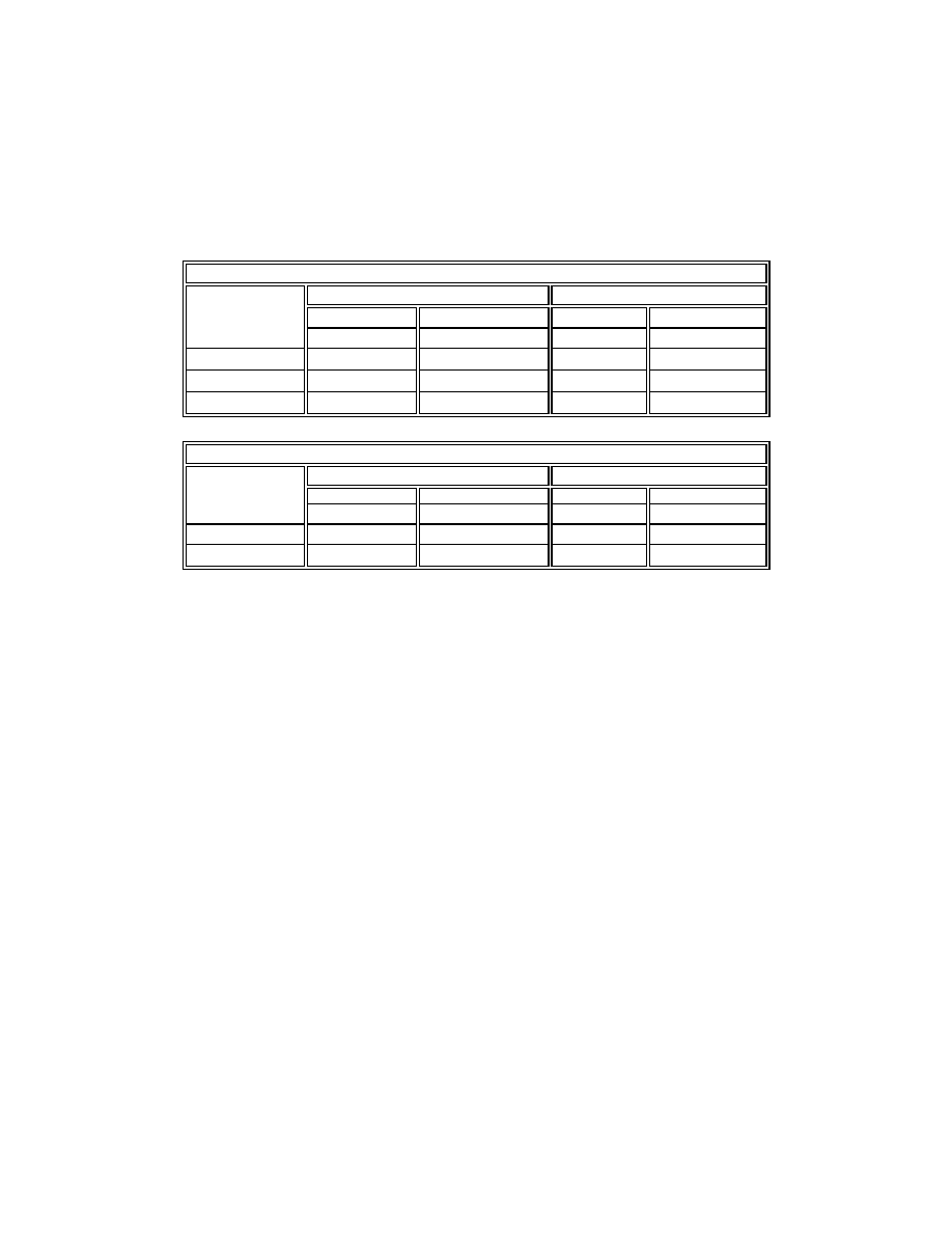
Emissions
The following tables show the savings in each emission component from installing GSHPs in lieu
of the conventional alternative. (Note: With all emissions results, a negative number indicates that
there are greater emissions of this component when GSHPs are employed).

Table 1 – Emissions Results – Green Bay

C O 2

S O 2

N O x

P a r t i c u l a

Large School

Emissions Reductions

8 5 2 , 3 4 1

- 1 , 1 0 6

1 6 8

- 5

- 0 . 0 0 2 9

Emissions Reductions (%)

13.88%

- 6 . 6 2 %

1 . 2 0 %

- 0 . 4 2 %

- 3 . 4 1 %

Emissions Reductions

2 . 1 9

-2.84 x10

- 3

4.31x10

- 4

-1.33 x

- 7 . 3 4

Small School

Emissions Reductions

1 9 0 , 0 4 5

- 5 2

1 3 6

0 . 0 0 0 2

Emissions Reductions (%)

15.40%

- 1 . 6 3 %

4 . 9 7 %

3 . 6 1 %

1 . 1 7 %

Emissions Reductions

2 . 7 5

-7.50 x10

- 4

1.96 x10

1.26 x10

- 4

2.74 x

Office

Emissions Reductions

1 4 1 , 8 9 4

- 3 6

1 0 4

1.49 x10

Emissions Reductions (%)

8 . 8 2 %

- 0 . 7 8 %

2 . 7 1 %

1 . 9 8 %

0 . 6 4 %

Emissions Reductions

2 . 0 6

-5.27 x 10

- 4

1.51 x10

9.91 x10

- 5

2.15 x10

Community Development (Mixed Residential)

Emissions Reductions

- 2 8 0 , 3 3 8

- 4 , 0 3 1

- 2 , 3 2 2

- 2 2 6

- 0 . 0 1 7 7

Emissions Reductions (%)

- 6 . 5 7 %

- 3 5 . 7 5 %

- 2 4 . 2 3 %

- 2 6 . 5 1 %

- 3 1 . 0 9 %

Emissions Reductions

- 1 . 5 2

-2.18 x10

- 2

- 1 . 2 5

-1.22 x10

Residential (Home)

Emissions Reductions

- 1 , 3 3 1

- 1 6

- 9

- 1

Emissions Reductions (%)

- 5 . 4 5 %

- 2 2 . 6 2 %

- 1 6 . 3 1 %

- 1 7 . 6 2 %

- 2 0 . 0 5 %

Emissions Reductions
( l b s / f t 2 )

- 0 . 9 7

-1.17 x10

- 2

- 6 . 9 0

x10

- 3

- 6 . 6 7 x 1 0

- 4

- 5 . 1 5

x10

- 8

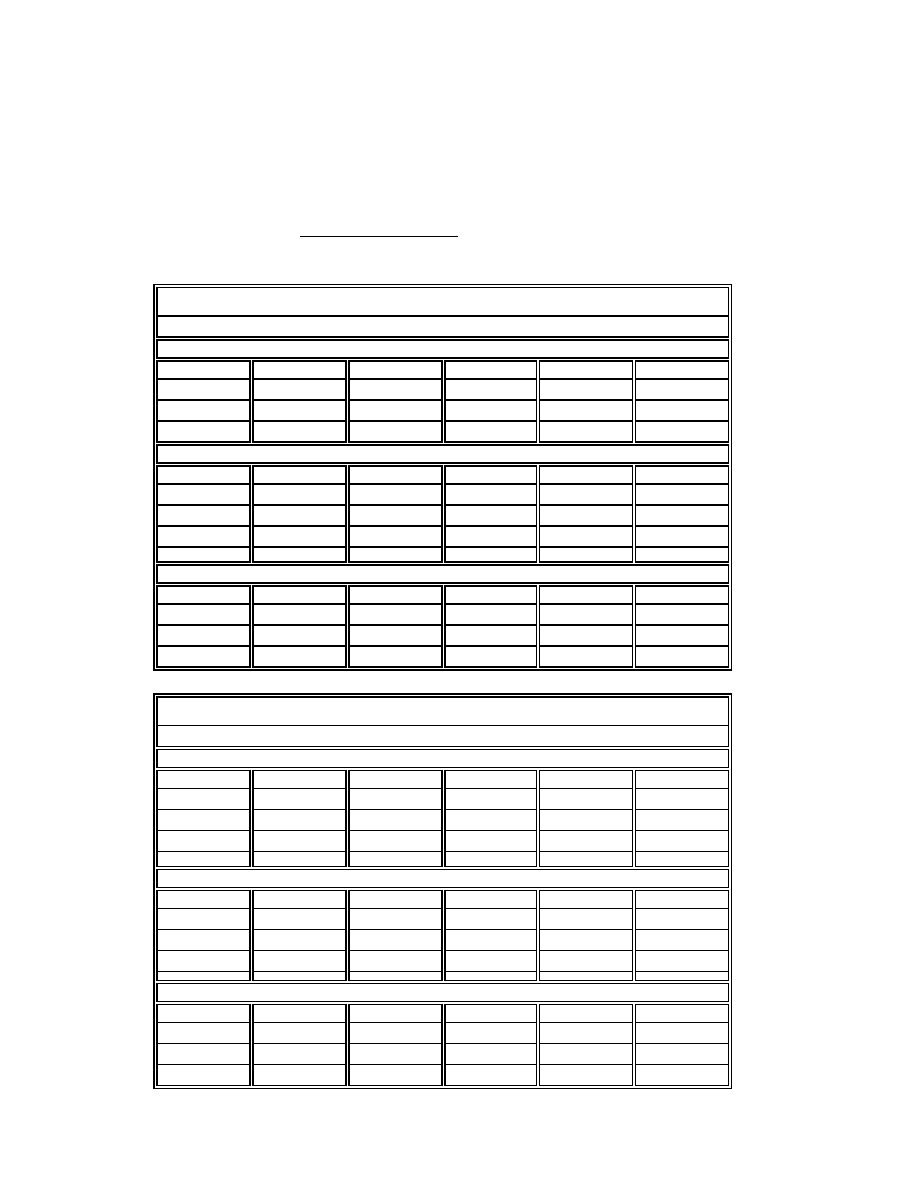
Table 2 – Energy & Economics Results – Green Bay

K W h s /

Y e a r

T h e r m s

/ Year

R e s o u r c e

( k B t u h s )

C o s t s

P a y b a

c k

P a y b a c k

w / R e a l

E s t a t e

Large School

Energy and Cost Savings

1 0 0 , 6 3 3

8 , 3 5 3 , 8 9 9 $ 3 5 , 5 9

9 . 8

1 . 6

Energy and Cost Savings

- 6 . 6 %

100.0%

23.2%

16.6%

Energy and Cost Savings

- 0 . 4 3

0 . 2 6

2 1 . 4

$ 0 . 0 9

Small School

Energy and Cost Savings

- 7 , 6 5 3

1 7 , 5 4 5

1 , 6 7 6 , 1 4 1

$ 5 , 4 0 6

2 4 . 3

1 4 . 7

Energy and Cost Savings
( % )

- 1 . 6 %

7 1 . 4 %

2 2 . 6 %

1 5 . 6 %

Energy and Cost Savings
(per ft2)

- 0 . 1 1

0 . 2 5

2 4 . 3

$ 0 . 0 8

Office

Energy and Cost Savings

- 5 , 1 5 0

1 2 , 9 9 7

1 , 2 4 6 , 9 6 9

$ 5 , 8 8 1

2 2 . 3

1 3 . 5

Energy and Cost Savings
( % )

- 0 . 7 %

7 0 . 2 %

1 4 . 7 %

1 3 . 2 %

Energy and Cost Savings
(per ft2)

- 0 . 0 7

0 . 1 9

1 8 . 1

$ 0 . 0 9

Community Development (Mixed Residential)

Energy and Cost Savings

7 7 , 9 0 1

1 , 5 3 9 , 0 5 7 $ 1 3 , 7 4

1 3 . 9

Energy and Cost Savings

- 3 5 . 6 %

1 0 0 . 0 %

6 . 1 %

8 . 6 %

Energy and Cost Savings

- 3 . 3 0

0 . 4 2

8 . 3 2

$ 0 . 0 7

Residential (Home)

Energy and Cost Savings

- 2 , 4 0 8

2 9 1

4 , 4 4 4

$ 7 5

2 4 . 1

Energy and Cost Savings

- 2 2 . 4 %

1 0 0 . 0 %

3 . 2 %

8 . 2 %

Energy and Cost Savings

- 1 . 7 6

0 . 2 1

3 . 2 4

$ 0 . 0 5

Discussion, Conclusions and Recommendations

The results summarized above imply that emissions reductions and customer economic benefits
depend on a complicated set of factors. These factors are discussed elsewhere in the report.
However, we can make some conclusions about the general viability of GSHPs in Wisconsin
based on the present mix of generation plants (i.e. this analysis is a snapshot in present time).

Economics

Emissions
The results show that there are significant reductions in CO

emissions from application of

GSHPs in the commercial sector. There are also typically small reductions in NO

and

particulates. However, there are typically small increases in SO

emissions. Finally, mercury

emissions are more variable in whether emissions increase or decrease; yet the levels of change are
very small for this pollutant.

The emissions results from use of GSHPs in Community Development and Residential
applications where natural gas is available show a different story. With one exception,
application of GSHPs in residential type buildings results in increased emissions as compared to
the conventional alternatives.

We ran the Community Development and Residential applications scenarios where natural gas is
not available and oil, LP gas or electric heating would be employed. The results of these analyses
are given in more detail later in the report. However, we can note that compared with LP gas the
results are similar to that of natural gas – increased emissions. Compared with oil and electric,
however, there are CO

reductions from the application of GSHPs in residential buildings.

Emissions Breakeven
The Center requested that we look at breakeven heating and cooling COP values for GSHPs such
that the CO

emissions savings are about zero. We performed a tertiary analysis for the Green

Bay Small School, Office, and Residential scenarios and found the following.

For commercial buildings the analysis shows that CO

emissions savings are positive for the

modeled buildings. Therefore, CO

emissions savings of zero can be achieved at lower COPs than

those found for our scenarios. The COPs found in our initial research approximate 3.0 for heating
and 3.6 for cooling. Our breakeven analysis suggests that CO

emissions savings would be about

zero given GSHP COPs of 2.4 for heating and 2.9 for cooling. This suggests that a reduction of
approximately 20% in heating and cooling COPs for the GSHP system would produce no CO

emissions savings for commercial buildings.

For residential buildings the analysis shows that CO

emissions savings are negative for the initial

modeling of the home HVAC requirements. In this case we needed to ask how high the heating
COP and cooling EER need to be for there to be no increases in CO

emissions. These efficiencies

would have to be raised to a heating COP of 5.1 and a cooling EER of 22.1 to reduce CO

emissions increases to zero. This pair of values is not technically achievable with present
technologies.

xii

Economics
For the Large School, the payback periods are good at between 7.1 and 10.5 years depending on
the city. The payback periods for installation of GSHPs in the Small School and the Office
building are two to four times longer (between 15.2 and 27.6 years).

This difference is primarily driven by the loop technology employed. The Large School is being
built in Fond du Lac in the near future and has been analyzed using a pond loop configuration –
the school needs these ponds to meet site drainage requirements. The Small School and Office
buildings were analyzed using vertical loops – which are significantly more expensive to install.

For the commercial type applications considered (schools, offices), we have also calculated the
payback from “real estate savings.” Where building owners see the value in reduced mechanical
room floor space requirements from not installing the conventional system, the payback periods
can be significantly shortened. For this analysis the Large School payback periods went down to
between 1.2 and 1.7 years. For the Small School and Office scenarios, the payback periods went
down to between 9.2 and 16.7 years.

Further, proponents of GSHP systems are confident that there are savings in O&M from
applying this technology. However, we can find no research to support this belief. Therefore, we
have not analyzed the impact of reduced O&M on payback periods.

The Community Development scenario has reasonable economics because the loop costs are
based on costs for an actual installation, in Louisiana. There, a large contract was let for loop
installations and economies of scale resulted in lower loop installation costs. Our analysis
suggests that for this scenario the payback periods range from 9.6 to 13.9 years.

The Residential scenario suggests long payback periods from application of GSHPs. This is due
to the low costs to install a simple furnace and A/C combination. Here the payback periods range
from 24.1 to 26.2 years.

Conclusions
There are significant emissions advantages to using GSHPs in the commercial sector. However,
there appear to be no emissions advantages to replacing efficient natural or LP gas furnaces with
GSHPs in the residential sector. There are emissions advantages in the residential sector when
GSHPs are compared to oil or electric heating in homes. These conclusions are based on current
mixes of utility power plants. Future changes in the power plant mixes will affect the results and
conclusions. In general, the lower the reliance on coal to generate electricity, the better will be the
emissions impact of installing GSHPs.

The payback periods for application of GSHPs in the residential sector are long , exceeding 20 or

xiii

more years in all cases. However, there are situations where GSHPs can be applied to commercial
buildings resulting in reasonable payback periods of less than 15 years. And, where real estate
savings are considered, the payback periods can shorten to less than two years for some
commercial applications.

Recommendations
While there are significant emissions advantages to using GSHPs in commercial buildings, the
economic analysis suggests there will need to be market supports to improve early economics
and develop significant, and possibly sustainable, market penetration.

We recommend that Public Benefits institutions and/or interested utilities provide programs to
help develop the infrastructure and market for GSHPs in the commercial sector.

It is clear the there are no environmental benefits to installing GSHPs in the residential sector in
colder climates where natural or LP gas is the alternative and coal is the primary fuel for power
plants. There are environmental benefits for homes where oil or electricity are the alternatives.

Given our findings, we recommend that Public Benefits institutions not spend much effort on
increasing the market share for GSHPs in the residential sector. However, we note an exception
to this suggestion if facilitating applications in the residential sector is required to build the
infrastructure so that capable contractors are available to install this technology in the commercial
sector. We also recommend this effort if the GSHPs will displace oil or electric heating in the
home.

Introduction

Introduction

History

Previous research indicates that Ground Source Heat Pumps (GSHP) provide superior HVAC
performance for all building types, while offering improved efficiency and lower operating costs
than conventional HVAC systems.

Various projects reviewing potential energy and energy cost savings for the installation of
GSHPs, in lieu of conventional technologies, reveal significant benefits. A general consensus in
the GSHP engineering industry indicates savings commonly in the order of 20% for commercial
buildings. Recent work by ASHRAE, the Ground Source Heat Pump Consortium, EPA and
others seems to substantiate this expectation. However, extant research, while conducted
throughout the United States, features fledgling or robust markets for GSHP systems; this does
not yet include Wisconsin.

The research reveals, as with many alternative technologies, a greater cost for installing GSHP
systems than for most conventional systems. While some GSHP proponents are quick to point
out exceptions (in some commercial buildings), the industry generally accepts a higher installation
cost for this less frequently specified technology. Prevailing research suggests an average cost
premium for installing GSHPs in commercial buildings between 10% and 20%. Typical cost
premiums in Wisconsin are uncertain because of limited experience with this technology. Indeed,
because of the lack of infrastructure, and the resultant “fears” of engineers toward applying this
technology, assistance may be initially necessary to ensure the installation of some early,
demonstrative systems.

The EPA has reported significant reductions in most emissions from the national deployment of
this technology, which has led the EPA and DOE to join forces in a variety of efforts to facilitate
the increased application of GSHP technologies. These organizations expect to invest in the
development of this technology in excess of $100 million between 1994 and 2004. Further, they
expect to facilitate an increase in annual installations from about 40,000 heat pumps per year, to
400,000 per year over the same time period.

Reports suggesting national capabilities for emissions reductions are encouraging. However, none
of these estimates apply specifically to Wisconsin. Theoretically, the confluence of weather
regimes and electric generation mixes could result in different emissions savings potential in
Wisconsin than the rest of the country at large.

Emissions and Economic Analysis of Ground Source Heat Pumps in Wisconsin

The Focus on Energy program, the Wisconsin Geothermal Association, and the Energy Center of
Wisconsin seek to learn how the emission and economic benefits apply to the application of this
technology in new buildings built throughout Wisconsin. Global Energy Options was retained to
develop estimates of economics and emissions impacts for a variety of application scenarios.

Approach

This report provides Wisconsin specific estimates of the impact on emissions from installing
GSHPs. It also provides estimates of economic benefits to building owners who install GSHPs
over the most appropriate conventional technology. We focus on the application of this
technology in new buildings.

We analyzed typical hourly energy use by the modeled buildings, and then compared this energy
use to the hourly operation of power plants throughout Wisconsin, assuming economic dispatch.
Our analysis includes buildings in three different climate regimes, served by three different
utilities. Modeling for five different building types results in fifteen scenarios. Our intense hourly
analysis ensures accurate results, hence ensuring a high degree of reliability upon which to base
policy decisions.

While this project was initially commissioned to determine the benefits of applying this
technology in the Focus on Energy territory (23 northeast counties served by WPS), we
ambitiously decided to expand the scope of the work to include the whole state. Today’s
modeling tools allowed us to cost effectively expand the scenarios to other weather regimes and
utility costing structures. And our choice of three different weather/utility points of analysis
allow for the interpolation of the results, somewhat reliably, to other parts of the state.

Originally we chose to analyze only four building types against our weather/utility dimension: a
school, an office, a community development, and a residence. However, CDH Energy was
conducting a feasibility study for a large school in Fond du Lac that is considering the GSHP
option. CDH Energy ran a DOE2 analysis of this building in the two other weather regimes for
us, adding a second school option for us to analyze.

What we Hoped to Learn

We hoped to determine if the application of GSHP technologies to buildings constructed in
Wisconsin offered environmental and economic benefits commensurate with the findings in other
parts of the North American continent.

We also hoped to determine if application of this technology afforded benefits to both the
commercial and residential new construction markets alike, or if application proved more
beneficial to one of these markets than to the other.

Introduction

Key Findings

The results show that there are significant reductions in CO

emissions from application of

GSHPs in the commercial sector. There are also typically small reductions in NO

and

Particulates. However, there are typically small increases in SO

emissions. Finally, mercury

emissions are more variable in whether emissions increase or decrease; yet the levels of change are
very small for this pollutant.

The emissions results from use of GSHPs to residential type applications shows a different
story. With one exception, application of GSHPs in residential type buildings results in increased
emissions as compared to the conventional alternatives.

The Community Development scenario has reasonable economics because the loop costs are
based on costs for a project implemented in Louisiana. There, a large contract was let for loop
installations and economies of scale resulted in lower loop installation costs. Our analysis
suggests that for this scenario the payback periods range from 9.6 to 13.9 years. This analysis
does not account for the additional cost of bringing a gas pipeline to the subdivision. If added,
the GHP payback period would be less.

Emissions and Economic Analysis of Ground Source Heat Pumps in Wisconsin

The Residential scenario suggests long payback periods for GSHPs. This is due to the low cost
to install a simple furnace and A/C combination. For the small house (1370 ft2) modeled here,
payback ranges from 24.1 to 26.2 years. Payback improves with increasing house size and loads.

Methods

Methods

Scenarios

We selected five building types and three weather regimes for which we have estimated
environmental and economic benefits. For analyzing the customer economics, we used rates for
the utility that serves each weather-regime city. Analyzing these dimensions results in fifteen
scenarios for which we provide results.

These scenarios are shown in the following table.

Table 3 - Scenarios for Which Analyses Were Performed

Building Type

Building Size (ft

)

Weather Location

Electric Utility

Large School

390,000

Green Bay

WPS

Large School

390,000

Madison

Alliant Energy

Large School

390,000

Eau Claire

NSP

Small School

69,000

Green Bay

WPS

Small School

69,000

Madison

Alliant Energy

Small School

69,000

Eau Claire

NSP

Office

69,000

Green Bay

WPS

Office

69,000

Madison

Alliant Energy

Office

69,000

Eau Claire

NSP

Community
Development

185,000

Green Bay

WPS

Community
Development

185,000

Madison

Alliant Energy

Community
Development

185,000

Eau Claire

NSP

Residence

1,370

Green Bay

WPS

Residence

1,370

Madison

Alliant Energy

Residence

1,370

La Crosse

NSP

The scope of the project did not allow us to model every commercial building type. We selected
schools and offices because these types of buildings are enjoying the most robust application of
GSHPs in other parts of the country.

Emissions and Economic Analysis of Ground Source Heat Pumps in Wisconsin

We added the community development scenario because we are aware of sustainable communities
that are assessing the use of GSHPs. ORNL has done significant analysis of projects of this type
in other parts of the country and found it easy to modify past modeling for Wisconsin building
code and weather parameters. A residential scenario is included to determine the benefits for this
market. The building sizes are functions of existing projects modeled by both ORNL and CDH
Energy.

We chose Green Bay, Madison, and Eau Claire because, from a state perspective, there are
reasonable differences among the weather regimes, and there are ASHRAE TMY (typical
meteorological year) data available for these cities. While a more northerly city like Rhinelander
would provide more diversity, no reliable weather data exists for that or nearby cities. The
heating degree-days (HDD) and cooling degree-days (CDD) estimates for each city are:

Table 4

C i t y

HDD

CDD

Madison

7 , 3 6 6

5 5 4

Green Bay

8 , 1 6 9

4 1 6

Eau Claire

8 , 4 1 7

5 0 5

La Crosse

7 , 8 1 4

8 3 4

Note: the Residential scenario analysis was conducted using La Crosse weather data because of
technical difficulties in TRANSYS using Eau Claire weather data.

Energy Use Analysis

GEO worked with ORNL and CDH Energy to develop hourly profiles of electric and gas
consumption for each of the scenarios analyzed. The proposed project included analysis from
ORNL for one residential and three commercial scenarios. Coincidentally, CDH Energy was
performing a feasibility analysis for a large school in Fond du Lac that was considering using
GSHPs, and participating in Alliant Energy’s Shared Savings program.

The Center asked GEO to add this school to its list of scenarios and asked CDH Energy to
provide 8760 hour energy use data to GEO. CDH Energy provided the data for the three weather
regimes considered.

Both ORNL and CDH Energy used DOE2 energy simulation software to develop energy use
profiles for the schools and the office. Profiles for the community development and residential
building scenarios were developed using TRANSYS. The building energy simulation industry
commonly uses and respects the reliability of both of these building energy use simulation
software packages.

As suggested earlier, we developed the profiles for the Large School scenarios based on a school

Methods

that will be built by the Fond du Lac school district in the next year. An existing school in
Lincoln, Nebraska forms the basis for the Small School scenario. ORNL has performed in-depth
comparisons of the Lincoln school with GSHPs to other identical schools in the Lincoln School
District to develop reliable comparisons of the school economics. ORNL modified the model
developed for this school to apply to Wisconsin commercial building code requirements and the
weather data for the three chosen cities.

For example, the prescriptive UAo values for commercial buildings under the building codes are
about those shown in the table below.

Maximum UAo for WI Commercial Buildings

Madison

Eau Claire

Green Bay

Roof Values

UAo =

0.051

0.047

0.049

R =

19.8

21.5

20.6

Above Grade Wall Values

UAo =

0.121

0.114

0.116

R =

8.2

8.7

8.6

Also, Wisconsin Commercial Building Code requires a minimum of 7.5 CFM per person for most
applications compared to ASHRAE 90.1, which suggests 15 CFM per person.

Similarly, the office building is based on an office in Tennessee for which ORNL has done
extensive HVAC technology comparison analyses. Again, we adjusted this building model for
Wisconsin commercial building code requirements and weather.

The Community Development scenario is based on a GSHP installation in Louisiana, which
includes where a variety of residential building types (mixed residential). The GSHPs replaced
standard air conditioning and gas furnaces. ORNL again chose to model this type of application
because it had done significant modeling and analysis of this project both before and after the
retrofit.

The home used for the residential scenario is located in Sun Prairie, Wisconsin, and was part of an
earlier Center project to look at the feasibility and economics of installing GSHPs in Wisconsin
homes. Data that ORNL could modify were available from earlier analyses of this home.

Using the building simulation models, ORNL and CDH Energy provided GEO with hourly
annual building kWh and therm uses. These two firms also used these energy uses to develop the
customer economics for these scenarios.

Emissions and Economic Analysis of Ground Source Heat Pumps in Wisconsin

HVAC equipment types and efficiencies

Some readers will want to know the efficiency assumptions used for the GSHPs and
conventional systems equipment. With the tools used to analyze HVAC options and energy use,
such as DOE2 and TRANSYS, equipment efficiency is not a single-point input. Instead, building
simulation experts use equipment performance tables from manufacturers.

However, when the simulation is completed, these experts are able to estimate the energy
weighted average efficiencies of the HVAC equipment. Rather than provide these estimates in
another section, we indicate them below.

Systems Modeled
We chose our base conventional system configurations based on what the market would typically
install for each type and size facility.

For the schools and office building, the base system is a water-cooled chiller with VAV/reheat
distribution system. The heating is provided using gas boilers. This includes winter heating load,
reheat as needed year round, and preheating ventilation air.

The GSHPs systems modeled for these buildings have separate heat pumps supplying space
heating and cooling to each defined zone. Most of these heat pumps are between 2 and 6 tons.
Some larger heat pumps are used for larger zones and to boost the temperature of make-up air.
These buildings do contain (smaller) gas boilers. These boilers are primarily needed for preheating
makeup air. This is because heat pumps are typically not designed to provide the necessary
temperature increase for the coldest Wisconsin winter days. The boilers might also provide heat
to some special areas like entrance vestibules if the design engineer uses this approach.

For all commercial buildings, regardless of the HVAC system installed, we assumed gas water
heating.

The Community Development scenario consists of a mix of various single family, duplex and
apartment buildings. The Residential scenario is based on a home in Sun Prairie in which a GSHP
was installed. Therefore, the base technologies for these scenarios are the same. We modeled
these buildings with furnaces and central air conditioning for the conventional base. For the
buildings modeled with conventional HVAC systems, we assumed the water heating is done by
gas. For the GSHP buildings, we assumed water heating is done by electric, with some of this
covered by an on-demand desuperheater.

Estimated average efficiencies
We have estimated the average efficiencies for each of the building and system types based on
BTU outputs and kWh or therm inputs (purchased). While there is some variation among the
cities because the weather varies a little over the year, we present an approximate number to

Methods

reflect the state average. These estimates are provided to allow the reader to get a sense of the
overall system efficiencies.

Table 5- Estimated Average Efficiencies: Commercial Buildings

Conventional System Efficiencies

GSHP System Efficiencies

Heating

Cooling

Heating

Cooling

Percent

kW/ton = EER

COP

COP = EER

Large School

7 8 %

1.4 = 8.6

3 . 3

3.1 = 10.6*

Small School

7 8 %

1.6 = 7.5

3 . 4

3.4 = 11.6

Office

7 8 %

1.4 = 8.6

3 . 0

3.6 = 12.3

Table 6- Estimated Average Efficiencies: Residential Type Buildings

Conventional System Efficiencies

GSHP System Efficiencies

Heating

Cooling

Heating

Cooling

Percent

EER

COP

EER

Community

9 2 %

1 2 . 4

3 . 3

1 3 . 2

Residential

9 2 %

1 2 . 0

3 . 5

1 7 . 0

*The CDH report for this building suggests that the modeling underestimates the cooling COP,
and believes that the actual cooling COP is higher than 3.1.

Emissions Analysis

While ORNL and CDH Energy were developing hourly energy use data, GEO developed a model
to estimate the impacts of these energy use profiles on emissions. As stated earlier, we chose to
analyze emissions from electricity use on an hourly basis to ensure confidence and reliability in
the environmental impact implications.

A major part of analyzing the viability of Ground Source Heat Pumps (GSHPs) is to determine
the amounts of pollutants emitted into the air during their use and to compare these emissions to
those of conventional HVAC systems. The aim of the analysis is to discern whether installing a
GSHP system in place of a conventional HVAC system reduces air emissions.

GEO developed three spreadsheet-based air emissions models representing the generation
characteristics of Alliant Energy, Wisconsin Public Service (WPS), and Northern States Power
(NSP) to calculate and compare air emissions between GSHP and conventional HVAC systems.
The models are similar to each other, and each uses the same process to calculate air emissions.
The only differences are the input data that represent a particular utility’s mix of generation, and
the specific hourly demand input data based on weather data for a city within each utility’s
service territory. Each air emissions model works as follows.

Emissions and Economic Analysis of Ground Source Heat Pumps in Wisconsin

Input data are first collected and placed in each model corresponding to the proper utility. The
input data include:

•

power plant unit characteristics such as nameplate capacity (MW), heat rate (Btu/kWh),
fuel cost (cents/kWh), and yearly outage data;

•

power plant air emissions factors in pounds per million Btu (lbs/MMbtu) for carbon
dioxide (CO

), sulfur dioxide (SO

), oxides of nitrogen (NO

), particulate matter, and

mercury (Hg). The model converts the emissions factors to lbs/kWh;

•

utility system hourly load data in MW for one year (8760 hours);

•

air emissions factors for natural gas, LP gas and oil combustion by HVAC equipment for
the above pollutants; and

•

hourly demand data in kW and therms over one year (8760 hours) for the GSHP and
conventional HVAC systems being compared.

More information on model input data is found in Appendix A.

Next, the model calculates how much energy in MWh each power plant unit contributes to
meeting the system demand for each hour of the year. This is done by first modifying the MW
capacity of each unit according to the percentage of generation that the utility owns, and reducing
the capacity according to (planned and unplanned) outage data. Then each power plant unit is
dispatched in order based first on fuel cost, then on heat rate, and then on MW capacity. In some
cases this dispatch order was modified to account for actual MWhs generated by a power plant,
according to historical information. If system demand cannot be met despite dispatching all of the
utility’s power plants, additional power plants representing bulk power purchases by the utility
are added to the dispatch. The characteristics and air emissions factors for these additional plants
are modeled based on a utility’s existing mix of generation. The energy produced due to bulk
power purchases constitute a small percentage of the total energy produced by the utility over
the year, hence they do not have a significant impact on air emissions results.

The energy produced by each power plant unit is then multiplied by the air emission factors to
determine the total amount of air pollutants each plant contributes in the test year. An average air
emission factor in lbs/kWh is then calculated for each pollutant.

The model then takes the hourly kW and therm data for the GSHP and conventional HVAC
systems being considered and calculates total electrical and natural gas energy used by these
systems over the year. The results are multiplied by the average air emissions factors to
determine the total number of pounds of air pollutants produced during the year when the GSHP
and conventional HVAC systems are operated. We then calculate the differences in total air
emissions between the two systems.

Methods

Daytypes
The air emissions model calculates the energy produced by the utility, average air emission
factors in lbs/kWh, and the energy used by the GSHP and the conventional HVAC systems
according to daytypes. Daytypes are a means of describing a utility system or demand-side
characteristic that corresponds to certain groups or categories of days during the year. For
example, a daytype called the Summer Weekday High could correspond to the one summer
weekday where system demand was highest.

A list of the daytypes used in the air emissions model and their abbreviations is shown in the
table below. This set of daytypes is one version that has been used by demand-side management
(DSM) planners in the past. Definitions of the daytypes used can be found in Appendix D.

Table 7 - Daytypes Used for Emissions Analysis

Winter

Summer

Spring/Fall

Weekday High

WWHigh

SWHigh

SFWHigh

Weekday Medium

WWMed

SWMed

SFWMed

Weekday Low

WWLow

SWLow

SFWLow

Weekend/Holiday All

WWHAll

SWHAll

SFWHAll

Emissions and Economic Analysis of Ground Source Heat Pumps in Wisconsin

Sensitivity Analysis
A sensitivity analysis was performed on the electric air emissions model to determine to what
degree differences in air emissions between a GSHP and a conventional HVAC system changed
when the dispatch order of the power plants changed. Two model runs using the original Large
School scenario kW and therm demand data in the Alliant Energy model were performed. The
first run dispatched power plants “properly,” meaning that the plants were dispatched first
according to fuel cost, then heat rate and power plant size. The second run dispatched power
plants “randomly,” without regard to fuel cost, heat rate, or plant size, although an overall
“rough” dispatch order was maintained where hydroelectric and nuclear plants were dispatched
first, followed by coal-fired plants, oil-fired plants, and natural gas-fired plants. This analysis
does not include gas use by the school as it is designed to test the sensitivity to power plant
dispatch assumptions.

The results of the sensitivity analysis shows (Table 8 below) that air emissions do not differ
greatly whether power plants are properly or randomly dispatched. This suggests that, while it is
important that all of a utility’s mix of generation is represented in the model, modeling how
power plants are dispatched with great accuracy (which can present many difficulties) is not
crucial when calculating air emissions.

Table 8

- Emissions Sensitivity Analysis

(1)

CO2

SO2

Particulate

Mercury

Proper Dispatch

(2)

(lbs)

-317,013

-1,900

-1,298

-57

-0.0069

Random Dispatch

(2)

(lbs)

-317,103

-1,847

-1,332

-59

-0.0069

Difference

(3)

(lbs)

-53

0.00%

Difference (%)

-0.028%

2.79%

-2.62%

-3.51%

0.00%

(1) Electric use considered only; does not include air emissions due natural gas combustion by the VAV Chiller systems
(2) Negative values mean that replacing the VAV Chiller with the GSHP results in increased air emissions.
(3) Differences in air emissions between proper and random dispatch cases are expressed with respect to proper dispatch.

The emission figures above are presented in terms of changes only for each type of pollutant
when comparing GSHPs to VAV/chiller/reheat systems. We simplified here because the tables
would have been too complex to also include totals. These indices will allow a variety of
audiences to gain insights regarding the emissions reductions capabilities of GSHPs in Wisconsin.

For each building/utility/weather scenario we present emissions savings of each type of pollutant.
Further, we estimate emissions reductions as a percentage of the emissions that would be created
by installing the GSHP system. This is provided to assist in comparing savings across building
types. Thus, negative values imply that the GSHP option will result in increased emissions of
that type.

Methods

Finally, we calculate emissions reductions per square foot of conditioned space to allow
comparison across building type and size.

Customer Economics

As with the emissions analysis, the economics analysis follows from the energy use analysis.
The 8760 demand profiles allowed us to apply the commercial rates for each utility to each of the
on-peak and off-peak hours for that utility.

The rates used for each utility are shown in the following table

Table 9

Rates Used for Economic Analyses

Rates

On-Pk Hrs

Off-Pk

Hrs

On-Pk

$ / k W h

Off-Pk
$ / k W h

On-Pk

$ / k W

Ratchet

$ / k W

$ / t h e r m

Large School

WPS

Estimated

8am-10pm

WkDays

A l l

Others

$ 0 . 0 2 7 3 $ 0 . 0 1 9 3

6 . 8 8

0 . 9 5

$ 0 . 3 8 9 1

Alliant

CP-1/Gc-2

8am-10pm

WkDays

A l l

Others

$ 0 . 0 2 8 8 $ 0 . 0 2 0 3

7 . 2 4

1 . 0 0

$ 0 . 4 5 0 0

NSP

Estimated

8am-10pm

WkDays

A l l

Others

$ 0 . 0 2 9 9 $ 0 . 0 2 1 1

7 . 5 3

1 . 0 4

$ 0 . 5 4 5 6

Small School

WPS

Cg-

1TOU/GRg

~8am-9pm

WkDays

A l l

Others

$ 0 . 0 3 4 7 $ 0 . 0 2 2 3

4 . 7 5

0 . 6 5

$ 0 . 3 6 5 8

Alliant

Cg-2/Gc-2

8am-10pm

WkDays

A l l

Others

$ 0 . 0 2 6 7 $ 0 . 0 2 6 7

5 . 7 5

1 . 0 0

$ 0 . 4 6 0 0

NSP

Cg-9/Gg-1

9am-9pm WkDays

A l l

Others

$ 0 . 0 3 8 5 $ 0 . 0 2 5 6

6 . 1 0

1 . 0 0

$ 0 . 5 2 5 0

O f f i c e

WPS

Cg-

1TOU/GRg

~8am-9pm

WkDays

A l l

Others

$ 0 . 0 3 4 7 $ 0 . 0 2 2 3

4 . 7 5

0 . 6 5

$ 0 . 3 6 5 8

Alliant

Cg-2/Gc-2

8am-10pm

WkDays

A l l

Others

$ 0 . 0 2 6 7 $ 0 . 0 2 6 7

5 . 7 5

1 . 0 0

$ 0 . 4 6 0 0

NSP

Cg-9/Gg-1

9am-9pm WkDays

A l l

Others

$ 0 . 0 3 8 5 $ 0 . 0 2 5 6

6 . 1 0

1 . 0 0

$ 0 . 5 2 5 0

C o m m u n i t y / R e s

WPS

Rg-1/CG-FM

- -

$0.0586 $0.0586

- -

$0.5080

Alliant

Gs-1/Gg-1

- -

$0.0593 $0.0593

- -

$0.5670

NSP

Rg-1/Rg-1

- -

$0.0671 $0.0671

- -

$0.5250

The next table shows the blended equivalent rates for each facility and technology scenario. The
blended rates for GSHPs are typically lower than for VAV/reheat systems because GSHPs have
lower peak monthly demands than VAV/reheat systems during the summer peak periods.

Emissions and Economic Analysis of Ground Source Heat Pumps in Wisconsin

Table 10 - Blended Rates

L a r g e
School

VAV Elect

GSHP Elec

VAV Gas

GSHP Gas

WPS

$ 0 . 0 6 9 0

$ 0 . 0 6 6 1

$ 0 . 3 8 9

$ 0 . 0 0 0

Alliant

$ 0 . 0 7 2 6

$ 0 . 0 6 9 5

$ 0 . 4 5 0

$ 0 . 0 0 0

NSP

$ 0 . 0 7 5 5

$ 0 . 0 7 2 3

$ 0 . 5 4 6

$ 0 . 0 0 0

S m a l l
School

VAV Elect

GSHP Elec

VAV Gas

GSHP Gas

WPS

$ 0 . 0 5 0 4

$ 0 . 0 5 1 7

$ 0 . 4 1 5

$ 0 . 5 3 6

Alliant

$ 0 . 0 5 3 0

$ 0 . 0 5 5 4

$ 0 . 4 8 0

$ 0 . 5 3 5

NSP

$ 0 . 0 5 5 1

$ 0 . 0 5 6 5

$ 0 . 5 8 2

$ 0 . 6 2 3

O f f i c e

VAV Elect

GSHP Elec

VAV Gas

GSHP Gas

WPS

$ 0 . 0 5 0 7

$ 0 . 0 4 9 6

$ 0 . 4 6 3

$ 0 . 5 8 3

Alliant

$ 0 . 0 5 3 6

$ 0 . 0 5 2 1

$ 0 . 5 0 3

$ 0 . 5 5 2

NSP

$ 0 . 0 6 2 9

$ 0 . 0 6 1 2

$ 0 . 6 0 0

$ 0 . 6 1 6

C o m m u n i t y

VAV Elect

GSHP Elec

Furnace Gas

GSHP Gas

WPS

$ 0 . 0 6 4 1

$ 0 . 0 6 2 6

$ 0 . 6 3 4

- -

Alliant

$ 0 . 0 6 4 2

$ 0 . 0 6 3 0

$ 0 . 6 7 0

- -

NSP

$ 0 . 0 7 2 5

$ 0 . 0 7 1 0

$ 0 . 7 3 1

- -

R e s i d e n t i a l

VAV Elect

GSHP Elec

Furnace Gas

GSHP Gas

WPS

$ 0 . 0 6 4 7

$ 0 . 0 6 3 6

$ 0 . 7 4 5

- -

Alliant

$ 0 . 0 6 5 4

$ 0 . 0 6 4 3

$ 0 . 7 7 1

- -

NSP

$ 0 . 0 7 3 2

$ 0 . 0 7 2 2

$ 0 . 8 5 6

- -

The economics presented later in this report are given in terms of savings only in electric and gas
costs, rather than in terms of total or partial facility costs with savings. We did this because
different energy accounting was used by CDH Energy and ORNL. While the modeling was done
differently, the results are equally valid and we report the savings only to prevent confusion.

CDH Energy modeled the energy use of most, but not all, components of the Large School
scenario. That is, they modeled energy use and costs of lighting & equipment, space heating &
cooling, and pumps and fans. However, they did not model water heating because gas would be
used equally to heat water with either HVAC system.

ORNL modeled the energy using systems differently. They modeled total facility energy and
several of the components - including HVAC, water heating, and dehumidification.

We have taken the economics information provided by CDH Energy and ORNL and synthesized
these into indices that we believe allow a variety of audiences to gain insights regarding the
economic viability of GSHPs in Wisconsin.

For each building/utility/weather scenario we analyzed total kWh and therm savings as well as
total annual energy cost savings and payback. Further, we estimate savings as a percentage of the

Methods

energy that would be used by the VAV system - including percentage of energy cost savings.
This is provided to assist in comparing savings across building types. Finally, we calculate
savings per square foot of conditioned space to allow comparison across building type and size.

Emissions and Economic Analysis of Ground Source Heat Pumps in Wisconsin

Results

Results

The results of this research are presented as a series of tables showing both the impact on
emissions and the economics of installing GSHPs in each of the five building types. Each table
represents a building type and within the tables the results for each of the city/utility/weather
scenarios are enumerated.

Each table therefore shows results for three sub-scenarios – representing each city/utility pair. In
addition the results are presented in three ways:

•

First we show the absolute emissions, energy and cost savings, and payback for each scenario

•

Below this, the results are presented in terms of percentage savings compared to the

conventional system emissions or energy and cost requirements

•

Finally, the results are presented on a square foot of conditioned space basis

We believe these presentation approaches will facilitate useful policy discussion.

Emissions Results

The following tables show the results of the emissions impacts where natural gas is the
alternative fuel for heating energy. These five tables are followed by tables showing the emissions
analyses where LP, oil, and electricity are assumed as the alternative heating fuel.

Table 11 - Large School Emissions Results

Natural Gas Heating

Sq. Ft. =

3 9 0 , 0 0 0

Emissions Reductions (pounds/year)

CO2

SO2

NOx

Particulate

Green Bay

8 5 2 , 3 4 1

- 1 , 1 0 6

1 6 8

- 5

- 0 . 0 0 2 9

Madison

6 5 1 , 5 3 3

- 1 , 5 0 7

- 2 6 3

- 0 . 0 0 3 5

Eau Claire

9 1 0 , 7 4 2

- 3 5 2

5 1 9

2 7

- 0 . 0 0 0 6

Emissions Reductions (%)

CO2

SO2

NOx

Particulate

Green Bay

1 3 . 8 8 %

- 6 . 6 2 %

1 . 2 0 %

- 0 . 4 2 %

- 3 . 4 1 %

Madison

1 1 . 5 6 %

- 5 . 4 1 %

- 1 . 3 1 %

0 . 9 8 %

- 3 . 4 3 %

Eau Claire

1 9 . 5 0 %

- 4 . 0 6 %

5 . 1 2 %

3 . 0 4 %

- 0 . 9 0 %

Emissions Reductions (pounds/ft2/year)

CO2

SO2

NOx

Particulate

Green Bay

2 . 1 9

- 2 . 8 4

4.31 x10

- 1 . 3 3

- 7 . 3 4

Madison

1 . 6 7

- 3 . 8 6

- 6 . 7 3

2.23 x10

- 9 . 0 7

Eau Claire

2 . 3 4 -9.0 x10

- 4

1.3 x10

- 3

6.9 x10

- 5

-1.5 x10

- 9

Emissions and Economic Analysis of Ground Source Heat Pumps in Wisconsin

Table 12 - Small School Emissions Results

Natural Gas Heating

Sq. Ft. =

6 9 , 0 0 0

Emissions Reductions (pounds/year)

CO2

SO2

NOx

Particulate

Green Bay

1 9 0 , 0 4 5

- 5 2

1 3 6

0 . 0 0 0 2

Madison

1 7 0 , 6 0 7

- 7 0

1 0 6

0 . 0 0 0 1

Eau Claire

1 9 2 , 9 3 4

- 7

1 5 8

1 1

0 . 0 0 0 3

Emissions Reductions (%)

CO2

SO2

NOx

Particulate

Green Bay

1 5 . 4 0 %

- 1 . 6 3 %

4 . 9 7 %

3 . 6 1 %

1 . 1 7 %

Madison

1 4 . 7 0 %

- 1 . 3 0 %

2 . 7 1 %

5 . 0 5 %

0 . 7 0 %

Eau Claire

1 9 . 8 3 %

- 0 . 4 4 %

7 . 8 7 %

6 . 2 0 %

2 . 6 5 %

Emissions Reductions (pounds/ft2/year)

CO2

SO2

NOx

Particulate

Green Bay

2 . 7 5

- 7 . 5 0

1.96 x10

1.26 x10

2.74 x10

Madison

2 . 4 7

- 1 . 0 1

1.54 x10

1.29 x10

2.03 x10

Eau Claire

2 . 8 0

- 1 . 0 7

2.30 x10

1.57 x10

4.72 x10

Table

13 - Office Emissions Results

Natural Gas Heating

Sq. Ft. =

6 9 , 0 0 0

Emissions Reductions (pounds/year)

CO2

SO2

NOx

Particulate

Green Bay

1 4 1 , 8 9 4

- 3 6

1 0 4

1.49 x10

Madison

1 2 4 , 2 4 2

2 2

1 1 8

3.37 x10

Eau Claire

1 3 4 , 8 3 5

- 5

1 1 0

1.84 x10

Emissions Reductions (%)

CO2

SO2

NOx

Particulate

Green Bay

8 . 8 2 %

- 0 . 7 8 %

2 . 7 1 %

1 . 9 8 %

0 . 6 4 %

Madison

8 . 0 7 %

0 . 2 7 %

2 . 0 7 %

3 . 1 5 %

1 . 1 5 %

Eau Claire

1 0 . 9 9 %

- 0 . 2 0 %

3 . 9 0 %

2 . 9 6 %

1 . 0 5 %

Emissions Reductions (pounds/ft2/year)

CO2

SO2

NOx

Particulate

Green Bay

2 . 0 6

- 5 . 2 7

1.51 x10

9.91 x10

2.15 x10

Madison

1 . 8 0

3.12 x10

1.71 x10

1.14 x10

4.89 x10

Eau Claire

1 . 9 5

- 7 . 3 1

1.59 x10

1.05 x10

2.67 x10

Results

Table 14 – Community Development Emissions

Natural Gas Heating

Sq. Ft. =

1 8 5 , 0 0 0

Emissions Reductions (pounds/year)

CO2

SO2

NOx

Particulate

Green Bay

- 2 8 0 , 3 3 8

- 4 , 0 3 1

- 2 , 3 2 2

- 2 2 6

- 0 . 0 1 7 7

Madison

- 2 2 5 , 8 2 0

- 6 , 4 6 3

- 3 , 7 2 3

- 1 4 3

- 0 . 0 2 1 7

Eau Claire

5 7 , 9 4 2

- 2 , 0 4 6

- 1 , 4 1 5

- 1 4 4

- 0 . 0 1 3 1

Emissions Reductions (%)

CO2

SO2

NOx

Particulate

Green Bay

- 6 . 5 7 %

- 3 5 . 7 5 %

- 2 4 . 2 3 %

- 2 6 . 5 1 %

- 3 1 . 0 9 %

Madison

- 5 . 4 2 %

- 3 3 . 5 0 %

- 2 6 . 3 4 %

- 2 2 . 5 1 %

- 3 0 . 0 3 %

Eau Claire

1 . 7 0 %

- 3 3 . 9 5 %

- 1 9 . 7 4 %

- 2 3 . 3 0 %

- 3 0 . 0 2 %

Emissions Reductions (pounds/ft2/year)

CO2

SO2

NOx

Particulate

Green Bay

- 1 . 5 2

- 2 . 1 8

- 1 . 2 5

- 1 . 2 2

- 9 . 5 6

Madison

- 1 . 2 2

- 3 . 4 9

- 2 . 0 1

- 7 . 7 1

- 1 . 1 7

Eau Claire

0 . 3 1

- 1 . 1 1 x

- 7 . 6 5

- 7 . 8 0

- 7 . 0 9

Table 15 - Residential Emissions Results

Natural Gas Heating

Sq. Ft. =

1 , 3 7 0

Emissions Reductions (pounds/year)

CO2

SO2

NOx

Particulate

Green Bay

- 1 , 3 3 1

- 1 6

- 9

- 1

- 7 . 0 5

Madison

- 1 , 2 1 4

- 2 5

- 1 5

- 1

- 8 . 5 7

La Crosse

- 1 1 5

- 7

- 5

- 1

- 4 . 7 2

Emissions Reductions (%)

CO2

SO2

NOx

Particulate

Green Bay

- 5 . 4 5 %

- 2 2 . 6 2 %

- 1 6 . 3 1 %

- 1 7 . 6 2 %

- 2 0 . 0 5 %

Madison

- 5 . 1 4 %

- 2 1 . 1 5 %

- 1 7 . 3 7 %

- 1 5 . 2 1 %

- 1 9 . 3 0 %

La Crosse

- 0 . 6 3 %

- 2 0 . 0 3 %

- 1 2 . 8 8 %

- 1 4 . 5 7 %

- 1 7 . 8 0 %

Emissions Reductions (pounds/ft2/year)

CO2

SO2

NOx

Particulate

Green Bay

- 0 . 9 7

- 1 . 1 7

- 6 . 9 0

- 6 . 6 7

- 5 . 1 5

Madison

- 0 . 8 9

- 1 . 8 5

- 1 . 0 9

- 4 . 2 3

- 6 . 2 5

La Crosse

- 0 . 0 8

- 5 . 4 3

- 3 . 9 4

- 3 . 9 0

- 3 . 4 5

Emissions and Economic Analysis of Ground Source Heat Pumps in Wisconsin

Residential options

where LP, oil, and electricity are assumed as the heating fuels for the

conventional systems.

Table 16 - Community Development Emissions Results

LP Gas Heating

Sq. Ft. =

1 8 5 , 0 0 0

Emissions Reductions (pounds/year)

CO2

SO2

NOx

Particulate

Green Bay

- 1 2 7 , 5 5 7

- 4 , 0 3 4

- 1 , 9 0 9

- 2 4 6

- 0 . 0 1 7 7

Madison

- 8 0 , 4 6 9

- 6 , 4 6 6

- 3 , 3 3 0

- 1 6 2

- 0 . 0 2 1 7

Eau Claire

2 1 5 , 6 6 2

- 2 , 0 4 9

- 9 8 8

- 1 6 5

- 0 . 0 1 3 1

Emissions Reductions (%)

CO2

SO2

NOx

Particulate

Green Bay

- 2 . 8 8 %

- 3 5 . 7 9 %

- 1 9 . 1 0 %

- 2 9 . 6 3 %

- 3 1 . 0 9 %

Madison

- 1 . 8 7 %

- 3 3 . 5 2 %

- 2 2 . 9 2 %

- 2 6 . 3 9 %

- 3 0 . 0 3 %

Eau Claire

6 . 0 5 %

- 3 4 . 0 2 %

- 1 3 . 0 2 %

- 2 7 . 6 5 %

- 3 0 . 0 2 %

Emissions Reductions (pounds/ft2/year)

CO2

SO2

NOx

Particulate

Green Bay

- 0 . 6 9

- 2 . 1 8

- 1 . 0 3

- 1 . 3 3

- 9 . 5 6

Madison

- 0 . 4 3

- 3 . 5 0

- 1 . 8 0

- 8 . 7 6

- 1 . 1 7

Eau Claire

1 . 1 7

- 1 . 1 1

- 5 . 3 4

- 8 . 9 4

- 7 . 0 9

Table 17 – Residential Emissions Results

LP Gas Heating

Sq. Ft. =

1 , 3 7 0

Emissions Reductions (pounds/year)

CO2

SO2

NOx

Particulate

Green Bay

- 7 6 1

- 1 6

- 8

- 1

- 7 . 0 5

Madison

- 6 9 5

- 2 5

- 1 4

- 1

- 8 . 5 7

LaCrosse

3 9 3

- 7

- 4

- 1

- 4 . 7 2

Emissions Reductions (%)

CO2

SO2

NOx

Particulate

Green Bay

- 3 . 0 4 %

- 2 2 . 6 4 %

- 1 3 . 3 0 %

- 1 9 . 3 8 %

- 2 0 . 0 5 %

Madison

- 2 . 8 8 %

- 2 1 . 1 6 %

- 1 5 . 4 8 %

- 1 7 . 3 5 %

- 1 9 . 3 0 %

LaCrosse

2 . 0 9 %

- 2 0 . 0 6 %

- 9 . 3 0 %

- 1 6 . 7 4 %

- 1 7 . 8 0 %

Emissions Reductions (pounds/ft2/year)

CO2

SO2

NOx

Particulate

Green Bay

- 0 . 5 6

- 1 . 1 7

- 5 . 7 7

- 7 . 2 3

- 5 . 1 5

Madison

- 0 . 5 1

- 1 . 8 5

- 9 . 8 7

- 4 . 7 3

- 6 . 2 5

LaCrosse

0 . 2 9

- 5 . 4 4

- 2 . 9 4

- 4 . 4 0

- 3 . 4 5

The following tables show the emissions analyses for the Community Development and

Results

Table 18 – Community Development Emissions

Fuel Oil Heating

Sq. Ft. =

1 8 5 , 0 0 0

Emissions Reductions (pounds/year)

CO2

SO2

NOx

Particulate

Green Bay

4 9 , 0 7 4

- 8 5

- 2 , 0 9 9

- 2 5 8

- 0 . 0 1 3 4

Madison

8 7 , 5 7 2

- 2 , 7 0 9

- 3 , 5 1 1

- 1 7 3

- 0 . 0 1 7 6

Eau Claire

3 9 8 , 0 0 4

2 , 0 2 8

- 1 , 1 8 5

- 1 7 8

- 0 . 0 0 8 7

Emissions Reductions (%)

CO2

SO2

NOx

Particulate

Green Bay

1 . 0 7 %

- 0 . 5 6 %

- 2 1 . 4 1 %

- 3 1 . 5 0 %

- 2 1 . 8 8 %

Madison

1 . 9 6 %

- 1 1 . 7 5 %

- 2 4 . 4 8 %

- 2 8 . 7 4 %

- 2 3 . 0 5 %

Eau Claire

1 0 . 6 3 %

2 0 . 0 8 %

- 1 6 . 0 2 %

- 3 0 . 3 1 %

- 1 8 . 0 2 %

Emissions Reductions (pounds/ft2/year)

CO2

SO2

NOx

Particulate

Green Bay

0 . 2 7

- 4 . 6 0

- 1 . 1 3

- 1 . 4 0

- 7 . 2 4

Madison

0 . 4 7

- 1 . 4 6

- 1 . 9 0

- 9 . 3 7

- 9 . 4 9

Eau Claire

2 . 1 5

1.10 x10

- 6 . 4 0

- 9 . 6 0

- 4 . 6 9

Table 19 - Residential Emissions Results

Fuel Oil Heating

Sq. Ft. =

1 , 3 7 0

Emissions Reductions (pounds/year)

CO2

SO2

NOx

Particulate

Green Bay

- 1 0 1

- 1

- 9

- 1

- 5 . 4 4

Madison

- 9 6

- 1 2

- 1 4

- 1

- 7 . 1 1

LaCrosse

9 8 1

- 5

- 1

- 3 . 2 9

Emissions Reductions (%)

CO2

SO2

NOx

Particulate

Green Bay

- 0 . 3 9 %

- 1 . 4 5 %

- 1 4 . 6 7 %

- 2 0 . 4 2 %

- 1 4 . 8 1 %

Madison

- 0 . 3 9 %

- 8 . 9 9 %

- 1 6 . 3 4 %

- 1 8 . 6 2 %

- 1 5 . 5 0 %

LaCrosse

5 . 0 5 %

1 1 . 3 2 %

- 1 0 . 9 2 %

- 1 8 . 0 2 %

- 1 1 . 7 7 %

Emissions Reductions (pounds/ft2/year)

CO2

SO2

NOx

Particulate

Green Bay

- 0 . 0 7

- 9 . 0 3

- 6 . 2 9

- 7 . 5 5

- 3 . 9 7

Madison

- 0 . 0 7

- 8 . 7 5

- 1 . 0 3

- 5 . 0 3

- 5 . 1 9

LaCrosse

0 . 7 2

4.15 x10

- 3 . 4 0

- 4 . 6 9

- 2 . 4 0

Emissions and Economic Analysis of Ground Source Heat Pumps in Wisconsin

Table 20 - Community Development Emissions

Electric Heating

Sq. Ft. =

1 8 5 , 0 0 0

Emissions Reductions (pounds/year)

CO2

SO2

NOx

Particulate

Green Bay

2 , 9 1 4 , 3 9

9 , 7 6 0

7 , 6 4 8

6 9 3

0 . 0 4 7 6

Madison

2 , 7 1 2 , 3 8

1 5 , 8 1 1

1 0 , 9 9 3

4 7 8

0 . 0 5 7 6

Eau Claire

2 , 1 8 8 , 7 9

5 , 4 1 1

5 , 6 8 7

5 0 1

0 . 0 3 6 8

Emissions Reductions (%)

CO2

SO2

NOx

Particulate

Green Bay

6 8 . 2 5 %

8 6 . 5 5 %

7 9 . 8 2 %

8 1 . 3 7 %

8 3 . 5 7 %

Madison

3 8 . 1 8 %

3 8 . 0 4 %

3 8 . 1 1 %

3 8 . 0 9 %

3 8 . 0 5 %

Eau Claire

3 9 . 5 4 %

4 0 . 1 3 %

3 9 . 8 6 %

3 9 . 6 1 %

3 9 . 3 4 %

Emissions Reductions (pounds/ft2/year)

CO2

SO2

NOx

Particulate

Green Bay

1 5 . 7 5

5.28 x10

4.13 x10

3.75 x10

2.57 x10

Madison

1 4 . 6 6

8.55 x10

5.94 x10

2.58 x10

3.11 x10

Eau Claire

1 1 . 8 3

2.92 x10

3.07 x10

2.71 x10

1.99 x10

Table 21 - Residential Emissions Results

Electric Heating

Sq. Ft. =

1 , 3 7 0

Emissions Reductions (pounds/year)

CO2

SO2

NOx

Particulate

Green Bay

1 0 , 5 9 9

3 6

2 8

1.73 x10

Madison

9 , 2 6 7

5 4

3 8

1.97 x10

LaCrosse

6 , 7 5 2

1 7

1.14 x10

Emissions Reductions (%)

CO2

SO2

NOx

Particulate

Green Bay

2 9 . 1 6 %

2 9 . 0 9 %

2 9 . 2 0 %

2 9 . 2 1 %

2 9 . 1 0 %

Madison

2 7 . 1 9 %

2 7 . 1 0 %

2 7 . 1 4 %

2 7 . 1 1 %

LaCrosse

2 6 . 8 2 %

2 7 . 1 2 %

2 6 . 9 8 %

2 6 . 8 6 %

2 6 . 6 9 %

Emissions Reductions (pounds/ft2/year)

CO2

SO2

NOx

Particulate

Green Bay

7 . 7 4

2.59 x10

2.03 x10

1.84 x10

1.26 x10

Madison

6 . 7 6 3.95 x10

- 2

2.74 x10

1.19 x10

1.44 x10

LaCrosse

4 . 9 3

1.21 x10

1.28 x10

1.13 x10

8.30 x10

Results

Emissions Breakeven

The Center requested that we look at breakeven heating and cooling COP values for GSHPs such
that the CO

emissions savings are about zero. We performed a simple analysis for the Green

Bay Small School and Office and the Residential scenarios only and found the following.

For commercial buildings the analysis shows that CO

emissions savings are positive for the

modeled buildings. Therefore, CO

emissions savings of zero can be achieved at lower COPs than

those found for our scenarios. The COPs found in our initial research approximate 3.0 for heating
and 3.6 for cooling. Our breakeven analysis suggests that CO

emissions savings would be about

zero given GSHP COPs of 2.4 for heating and 2.9 for cooling. This suggests that a reduction of
approximately 20% in heating and cooling COPs for the GSHP system would produce no CO

emissions savings for commercial buildings.

For residential buildings the analysis shows that CO

emissions savings are negative for the initial

modeling of the home HVAC requirements. In this case we needed to ask how high the heating
COP and cooling EER need to be for there to be no increases in CO

emissions. These efficiencies

would have to be raised to a heating COP of 5.1 and a cooling EER of 22.1 to reduce CO

emissions increases to zero. This pair of values is not technically achievable.

Economics Results

The following tables show the results of the economics analyses.

The “Payback-Energy Only” figures show the payback when only energy savings are considered
in calculating the payback.

The “Payback-w/Real Estate” figures show the payback including both energy savings and real
estate cost savings from installing GSHPs. (Based on 1.5% of the floor area freed up and $50/ft2
unfinished construction costs).

There are no “Payback-w/Real Estate” figures for the Community Development and Residential
building types because there are no real estate savings for these scenarios.

Emissions and Economic Analysis of Ground Source Heat Pumps in Wisconsin

Table 22- Large School Energy & Economics Results

Sq. Ft. =

3 9 0 , 0 0 0

Incremental Costs =

$ 3 5 0 , 0 0 0

Energy and Cost Savings (Annual)

kWhs

Therms

Resource

(kBtuhs)

Energy Costs

Payback –

Energy Only

Payback –

w/Real Estate

Green Bay

- 1 6 6 , 9 5 0

1 0 0 , 6 3 3

8 , 3 5 3 , 8 9 9

$ 3 5 , 5 9 0

9 . 8

1 . 6

Madison

- 1 3 2 , 4 9 9

7 7 , 2 2 4

6 , 3 6 5 , 7 4 3

$ 3 3 , 2 2 8

1 0 . 5

1 . 7

Eau Claire

- 1 2 6 , 1 0 6

9 2 , 1 0 4

7 , 9 1 9 , 2 0 1

$ 4 9 , 3 4 3

7 . 1

1 . 2

Energy and Cost Savings (%)

kWhs

Therms

Resource

(kBtuhs)

Energy Costs

Green Bay

- 6 . 6 %

100.0%

23.2%

16.6%

Madison

- 5 . 3 %

100.0%

19.2%

15.5%

Eau Claire

- 5 . 0 %

100.0%

22.5%

20.4%

Energy and Cost Savings (per ft2/year)

kWhs

Therms

Resource

(kBtuhs)

Energy Costs

Green Bay

- 0 . 4 3

0 . 2 6

2 1 . 4

$ 0 . 0 9

Madison

- 0 . 3 4

0 . 2 0

1 6 . 3

$ 0 . 0 9

Eau Claire

- 0 . 3 2

0 . 2 4

2 0 . 3

$ 0 . 1 3

Table 23 – Small School Energy & Economics Results

Sq. Ft. =

6 9 , 0 0 0

Incremental Costs =

$ 1 3 1 , 0 0 0

Energy and Cost Savings (Annual)

kWhs

Therms

Resource

(kBtuhs)

Energy Costs

Payback –

Energy Only

Payback –

w/Real Estate

Green Bay

- 7 6 5 3

1 7 5 4 5

1 , 6 7 6 , 1 4 1

$ 5 , 4 0 6

2 4 . 3

1 4 . 7

Madison

- 5 5 9 2

1 5 5 1 9

1 , 4 9 4 , 6 4 4

$ 5 , 6 8 1

2 3 . 1

1 4 . 0

Eau Claire

- 4 3 4 1

1 6 9 2 9

1 , 6 4 8 , 4 5 3

$ 8 , 6 2 3

1 5 . 2

9 . 2

Energy and Cost Savings (%)

kWhs

Therms

Resource

(kBtuhs)

Energy Costs

Green Bay

- 1 . 6 %

7 1 . 4 %

2 2 . 6 %

1 5 . 6 %

Madison

- 1 . 2 %

7 3 . 4 %

2 1 . 3 %

1 6 . 0 %

Eau Claire

- 0 . 9 %

6 9 . 6 %

2 2 . 2 %

2 1 . 1 %

Energy and Cost Savings (per ft2/year)

kWhs

Therms

Resource

(kBtuhs)

Energy Costs

Green Bay

- 0 . 1 1

0 . 2 5

2 4 . 3

$ 0 . 0 8

Madison

- 0 . 0 8

0 . 2 2

2 1 . 7

$ 0 . 0 8

Eau Claire

- 0 . 0 6

0 . 2 5

2 3 . 9

$ 0 . 1 2

Results

Table 24 – Office Energy & Economics Results

Sq. Ft. =

6 9 , 0 0 0

Incremental Costs =

$ 1 3 1 , 0 0 0

Energy and Cost Savings (Annual)

kWhs

Therms

Resource

(kBtuhs)

Energy Costs

Payback –

Energy Only

Payback –

w/Real Estate

Green Bay

- 5 1 5 0

1 2 9 9 7

1 , 2 4 6 , 9 6 9

$ 5 , 8 8 1

2 2 . 3

1 3 . 5

Madison

2 7 5 4

1 0 1 8 7

1 , 0 4 6 , 8 9 8

$ 6 , 1 1 8

2 1 . 4

1 3 . 0

Eau Claire

- 5 4 0 7

1 2 0 1 4

1 , 1 4 6 , 0 3 8

$ 7 , 9 8 7

1 6 . 4

9 . 9

Energy and Cost Savings (%)

kWhs

Therms

Resource

(kBtuhs)

Energy Costs

Green Bay

- 0 . 7 %

7 0 . 2 %

1 4 . 7 %

1 3 . 2 %

Madison

0 . 4 %

6 9 . 1 %

1 2 . 6 %

1 4 . 1 %

Eau Claire

- 0 . 8 %

6 6 . 7 %

1 3 . 5 %

1 5 . 4 %

Energy and Cost Savings (per ft2)

kWhs

Therms

Resource

(kBtuhs)

Energy Costs

Green Bay

- 0 . 0 7

0 . 1 9

1 8 . 1

$ 0 . 0 9

Madison

0 . 0 4

0 . 1 5

1 5 . 2

$ 0 . 0 9

Eau Claire

- 0 . 0 8

0 . 1 7

1 6 . 6

$ 0 . 1 2

Table 25 - Community Development Energy & Economics

Sq. Ft. =

1 8 5 , 0 0 0

Energy and Cost Savings (Annual)

kWhs

Therms

Resource

(kBtuhs)

Energy Costs

Payback

Green Bay

- 6 1 0 5 1 3

7 7 9 0 1

1 , 5 3 9 , 0 5 7

$ 1 3 , 7 4 7

1 3 . 9

Madison

- 5 7 3 8 8 4

7 4 1 1 3

1 , 5 3 5 , 3 0 2

$ 1 5 , 5 7 8

1 2 . 2

Eau Claire

- 6 3 9 3 1 9

8 0 4 2 0

1 , 4 9 6 , 0 1 3

$ 1 5 , 9 9 4

1 1 . 9

Energy and Cost Savings (%)

kWhs

Therms

Resource

(kBtuhs)

Energy Costs

Green Bay

- 3 5 . 6 %

1 0 0 . 0 %

6 . 1 %

8 . 6 %

Madison

- 3 3 . 1 %

1 0 0 . 0 %

6 . 0 %

9 . 4 %

Eau Claire

- 3 6 . 9 %

1 0 0 . 0 %

5 . 8 %

8 . 7 %

Energy and Cost Savings (per ft2)

kWhs

Therms

Resource

(kBtuhs)

Energy Costs

Green Bay

- 3 . 3 0

0 . 4 2

8 . 3 2

$ 0 . 0 7

Madison

- 3 . 1 0

0 . 4 0

8 . 3 0

$ 0 . 0 8

Eau Claire

- 3 . 4 6

0 . 4 3

8 . 0 9

$ 0 . 0 9

Emissions and Economic Analysis of Ground Source Heat Pumps in Wisconsin

Table 26 – Residential Energy & Economics Results

Sq. Ft. =

1 , 3 7 0

Energy and Cost Savings (Annual)

kWhs

Therms

Resource

(kBtuhs)

Energy Costs

Payback

Green Bay

- 2 4 0 8

2 9 1

4 , 4 4 4

$ 7 5

2 4 . 1

Madison

- 2 2 7 6

2 6 4

3 , 0 9 6

$ 6 9

2 6 . 2

La Crosse

- 2 2 5 4

2 5 9

2 , 8 2 1

$ 7 0

2 5 . 8

Energy and Cost Savings (%)

kWhs

Therms

Resource

(kBtuhs)

Energy Costs

Green Bay

- 2 2 . 4 %

1 0 0 . 0 %

3 . 2 %

8 . 2 %

Madison

- 2 1 . 2 %

1 0 0 . 0 %

2 . 3 %

7 . 6 %

La Crosse

- 2 0 . 9 %

1 0 0 . 0 %

2 . 1 %

6 . 9 %

Energy and Cost Savings (per ft2/year)

kWhs

Therms

Resource

(kBtuhs)

Energy Costs

Green Bay

- 1 . 7 6

0 . 2 1

3 . 2 4

$ 0 . 0 5

Madison

- 1 . 6 6

0 . 1 9

2 . 2 6

$ 0 . 0 5

La Crosse

- 1 . 6 5

0 . 1 9

2 . 0 6

$ 0 . 0 5

Discussion

Discussion

Introduction

The research reveals, as with many alternative technologies, a greater cost for installing GSHP
systems than for most conventional systems. While some GSHP proponents are quick to point
out exceptions, (in some commercial buildings), the industry generally accepts that there will be a
higher installation cost for this less frequently specified technology. Prevailing research suggests
an average cost premium for installing GSHPs in commercial buildings between 10% and 20%.
Typical cost premiums in Wisconsin are uncertain because of limited experience with this
technology. Indeed, because of the lack of infrastructure, and the resultant “fears” of engineers
toward applying this technology, assistance may be initially necessary to ensure the installation
of some early, demonstrative systems.

Reports suggesting national capabilities for emissions reductions is encouraging. However, none
of these estimates apply specifically to Wisconsin. Theoretically, the confluence of weather
regimes and electric generation mixes could result in different emissions savings potential in
Wisconsin than the rest of the country.

Interpretation of Results

The tables in the previous section indicate varying results in terms of both emissions reductions
and economics.

Emissions and Economic Analysis of Ground Source Heat Pumps in Wisconsin

Emissions
There is a clear dichotomy between commercial and residential types of buildings with regard to
the potential for reducing emissions by installing GSHPs. Commercial buildings reduce most
emissions (but not all) while residential applications result in increased emissions when GSHPs
are installed where NG is available.

We believe this primarily is a function of air conditioning requirements and secondarily impacted
by base technology differences.

Air conditioning requirements are substantially higher in commercial buildings than in residential
buildings throughout the U.S. This is primarily driven by the internal gains in commercial
buildings from lighting, equipment (increasingly computers), and people loads (and required
ventilation). Conversely, air conditioning requirements in residential buildings is much lower.

The emissions reductions in commercial buildings are primarily driven by substituting GSHP
systems that provide cooling comfort at higher efficiencies than the alternative VAV/reheat
systems that would have been installed.

The reason Wisconsin residential buildings using GSHPs produce more emissions is that heating
is shifted from “cleaner” gas to “dirtier” electric, and there is too little cooling to reduce emissions
(through higher SEERs) to offset increases in emissions from this shift of heating fuel.

As we look south, the heating load decreases and cooling requirements increase. Therefore, it is
not hard to understand that while GSHPs increase emissions in homes in the northern tier of the
country, they may be effective at decreasing emissions in residential building applications south
of Wisconsin.

Another Wisconsin reality that results in negative emissions impact from GSHPs in the
residential sector compared to the commercial sector is the preponderance of high efficiency
furnaces. We modeled the residential scenarios assuming a condensing furnace would have been
installed if the GSHP system was not. Thus less gas is burned reducing the emissions for the base
case in the residential sector. On the other hand, the typical boilers installed in commercial
buildings are about 80% efficient. Shifting this inefficient gas heating to more efficient heat pump
heating provides more emissions reductions per square foot than in the residential buildings.

Again, as we look south, more 80% efficient furnaces are installed in homes – improving the
emissions reductions from installing GSHPs.

Discussion

Breakeven Emissions
While our breakeven analysis is not robust, it does provide some insights into systems
capabilities for emissions savings.

For commercial buildings the analysis shows that CO

emissions savings can be achieved for

GSHP COPs as low as about 2.4 for Heating, and 2.9 for Cooling (~20% lower than modeled).
Thus, with incentives, there would be room for scaling the incentives to the system efficiencies
above some minimal COPs. We suggest that if such scaling is considered, a more robust analysis
than we performed should be conducted.

The results also show that for residences, there is no breakeven against the furnace and central
A/C combination in Wisconsin. This is because there is not enough air conditioning load in
Wisconsin homes to provide the CO

emissions reductions to overcome the CO

emissions

increase from shifting gas heating to electric (albeit high efficiency) in the home. We believe that
the CO

emissions savings can be achieved for some homes somewhere south of Illinois. We

suggest that there is no reason to develop any direct incentives for installing GSHPs in Wisconsin
homes. However, our experience suggests that programs that improve HVAC contractors’
capabilities and confidence with this technology improve the infrastructure needed to install
GSHP systems in commercial buildings.

Economics
Estimating economics is a little more slippery than estimating emissions savings capabilities, due
to many more potentially confounding factors. One primary assumption is the type of loop field
installed for the GSHP system. There are many others that can result in an incremental cost
increase for the GSHP system from 0% to 40% above the cost of the conventional system. The
most commonly accepted average cost increase is about 20% for commercial buildings.

The tables in the previous section show the payback periods for each of the scenarios modeled. It
is easily observed that the payback periods vary widely. There are logical reasons for this.

Large School - The Large School scenarios are based on a system that has recently been
approved to be installed in a 390,000 ft

school in Fond du Lac, Wisconsin. This school has the

good fortune (from a GSHP perspective) of having to install a couple of large area (and 20 feet
deep) runoff retention ponds. These ponds allow the school to install pond loops rather than the
typical vertical loop system.

Because of this, the incremental cost is only $350,000 (which is not high given the size of the
school). This low incremental cost leads to payback periods of between 7.1 and 10.5 years.
When the building owner sees value in the utilization of floor space that would otherwise have

Emissions and Economic Analysis of Ground Source Heat Pumps in Wisconsin

been allocated to the VAV/reheat systems, the payback periods are in the order of 1.2 to 1.7
years.

Small School and Office - The payback periods for the Small School and Office scenarios are
noticeably longer: Between 15.2 and 24.2 years for the Small School and between 20.0 and 27.6
years for the Office.

The primary reason that these payback periods are longer is that the incremental cost for
installing the GSHP system is significantly higher. This is true because ORNL modeled these
systems with vertical loops (as opposed to the pond loop in the Large School scenario). It is
reasonable to assume that vertical loops might be installed in many cases because this is the most
common loop configuration for commercial buildings.

Where the building owner accepts the real estate benefit of this technology, the payback periods
become more reasonable: Between 9.2 and 14.7 years for the Small School and between 12.1 and
16.7 years for the Office. Real estate benefit is derived from the reduced mechanical room floor
space requirements afforded by installing GSHPs.

It should be noted that the Small School scenario is modeled after systems installed in the Lincoln
(Nebraska) School District. It has been shown that the GSHP system installation at several
schools in this district were installed for the same cost as VAV/reheat systems installed in other
schools in the district. That is, the incremental cost was $0 – providing an immediate payback.
Thus, while typical, the long payback periods we present in this analysis do not preclude cases
where the payback periods might be much shorter.

Community Development – The payback periods for the Community Development scenarios are
reasonable compared to the residential scenario, even though this application is primarily
residential in nature. The reason for this is that ORNL has experience that shows that when a
large community GSHP project is bid out in whole, the cost of installing the loops for a
community scenario can be significantly reduced. It is clear, as with any non-standard
technology, that the cost to install GSHPs is high until an infrastructure is developed to design
and install the technology – leading to confidence, competence and competition.

Based on energy savings alone the payback periods range between 11.9 and 13.9 years. There is
no real estate value from employing GSHPs in this and the residential sector. That is because the
GSHP air handler takes as much room as a furnace and the value of basement space in a home
does not hold the value of commercial space.

Residential – In this study, GSHPs do not offer environmental benefits for the typical home; the
economics also are not favorable. The 24.1 to 26.2 year payback periods may make this

Discussion

technology appear risky to most homeowners. However, because the cost of the system will be
put in the new home mortgage, the homeowner can see a positive cash flow from this technology.

Impactors
There are a variety of parameters that impact the difference in emissions and economics across
the scenarios. These impactors also play a role in the viability of this technology in Wisconsin
compared to other states.

Weather – Wisconsin’s cooler climate lowers the potential emissions reductions and lengthens
the payback periods.

Research shows that warmer weather improves the emissions reductions and economics of
installing GSHPs. This is because more air conditioning results in more emissions savings from
cooling to offset the emissions increase from shifting heating from gas to electricity (albeit
efficient electric heating).

The emissions and economics advantages of GSHPs are greater as one moves south.

Ventilation Requirements – Wisconsin’s ventilation code requirements are lower than those
recommended by ASHRAE Standard 62, lowering the potential emissions reductions and
lengthening the payback periods.

ASHRAE 62 – 1989 recommends a typical 15 cubic feet per minute (CFM) of ventilation per
person in many commercial spaces. The new Wisconsin Commercial Building code allows
engineers to design for 7.5 CFM per person. This lowers the ventilation air heating and cooling
requirements and reduces the energy savings over what they would be if the buildings were
designed for 15 CFM per person.

The Large School scenario analysis is based on 15 CFM while the other scenarios are based on
7.5 CFM. If the Small School and Office buildings were modeled with 15 CFM, the emissions
and economic results would likely improve slightly to moderately.

Conventional system application – The viability of GSHPs in the residential sector is challenged
by the saturation of condensing furnaces installed in the Wisconsin market.

In the commercial sector installed boilers typically operate at about 80% efficiency. This tends to
improve the emissions and economics capabilities compared to the residential sector. As a result
of many years of utility energy efficiency programs, about 85% of furnaces installed in
Wisconsin homes are condensing – with an efficiency of greater than 90%.

Emissions and Economic Analysis of Ground Source Heat Pumps in Wisconsin

This and the high levels of construction requirements in the residential building code have reduced
the energy requirements for both heating and cooling to a level that forces a long payback period
for the incremental cost of installing the GSHP loop.

Electric and gas commodity costs – The low costs of electricity and gas in Wisconsin has a
negative impact on the economics of GSHPs.

GSHP systems are installed more frequently in parts of the country that have high electric and
gas costs. This is because the economics of this system depend on saving on energy costs. Where
the costs of energy are higher, the savings are high for a given percentage of energy use
reductions.

Our analysis is based on present costs of electric and gas to Wisconsin building owners. This
analysis does not account for a potential greater escalation of gas rates compared to electric rates.
Some believe that laying the infrastructure of gas piping throughout Wisconsin will result in gas
rates increasing faster than electric. This would tend to tilt the economics in favor of GSHP
systems.

Generation mix – Wisconsin’s mix of generating plant types is typical. This mix results in
emissions savings, from installing GSHPs, that are likely typical in other parts of the U.S with
similar weather regimes.

The cleaner and greener the electricity generation, the greater the emissions savings potential are
likely to be from application of GSHPs. That is, where larger fractions of the total MWh
generation are produced by hydro, wind, and nuclear, the emissions savings potential from this
technology are likely to be greater compared to using gas heating.

Technology Infrastructure – It is generally accepted that the lack of technology infrastructure to
specify, design and install GSHPs results in higher cost of installation of these systems in
Wisconsin compared to the conventional alternatives.

States that are interested in the public benefits of GSHPs are investing in building the local
infrastructure for the technology with the expectation that the cost premiums will be reduced and
the technology will become more competitive.

Value of real estate – GSHP systems infringe upon less of the conditioned space than to
VAV/reheat systems. Where the Wisconsin building owner sees this value, this can improve the
economics of installing this technology.

Discussion

For schools, this freed up area can result in lower building costs if considered at the design stage
of the construction of the new building. Or the school might see value in having more classroom
or common space.

For the office, this space can easily translate to more rentable space – translating into higher rent
income. In Madison, space in newer buildings is presently running between $14 and $18 per ft

per year. This can be significant. For example, a 69,000 ft

office renting out at $15/ ft

/year and

renting an additional 1.5% of this space out can reduce the payback period from the 20.0 to 27.6
years suggested earlier to 5.9 to 6.5 years.

Conclusions

This research suggests that there is significant potential reduction of most emissions from
installing GSHPs in at least some types of commercial buildings. The results also show that
installing GSHPs in residential-type buildings results in increased emissions where natural or LP
gas is the alternative. Where oil or electric heating is the alternative, there are potential emissions
reductions in the residential sector.

The economics analyses also show that for many cases the payback periods from installing
GSHPs in both commercial and residential buildings can be high when energy benefits alone are
considered. These payback periods are significantly shortened where the building owner sees the
benefit of having to construct less square footage for the equivalent public or commercial
enterprise, or if this space can be rented out instead of containing the air handling units.

Recommendations

Based on the results of this work, we believe commercial GSHP systems should be considered in
programs that will be delivered under the Public Benefits. We also believe some utilities might be
interested in including this technology in their commercial energy efficiency program portfolios.
These recommendations are based on the fact that while there are environmental benefits to
installing GSHPs in commercial buildings, the payback periods for many potential applications
may be somewhat long and education and incentive programs may be needed to facilitate the
development of a sustainable market for GSHPs in Wisconsin.

We do not see any direct reason for promoting residential GSHP systems where natural or LP gas
are available. However, it may be appropriate to promote this technology where the alternative
heating fuels are oil or electricity. Also, there may be a short term indirect reason for promoting
this technology in the residential sector. We have observed that in most parts of the country
where this technology is building momentum, the infrastructure was built by first training HVAC
and loop contractors in the residential sector. After these local contractors gain confidence in the
residential sector, they find it easier to graduate to installing the systems in commercial buildings.

Emissions and Economic Analysis of Ground Source Heat Pumps in Wisconsin

If the Public Benefits industry finds it difficult to build direct commercial capabilities, it might
consider starting in the residential sector – with the goal of not supporting residential systems
when the commercial system infrastructure is adequate.

Limitations and Future Research

Our research was necessarily limited to a few building type and HVAC system configuration
scenarios. There are a variety of other commercial building types in which GSHPs might be
installed. It is uncertain that the emissions and economics results shown here can be applied
accurately to other building types (such as health care, restaurant, etc).

Also, the GSHP system costs used by ORNL were taken from other parts of the country and
adjusted for Wisconsin. Other cost considerations might arise that could impact the economics.

Further, all of this work is based on modeled energy use for each scenario. While, the ORNL
analyses were calibrated to actual billing data for actual buildings they have researched, it is not
certain that the energy and economic results are fully transferable to Wisconsin.

Finally, we compared the GSHP systems to only VAV/reheat systems in this work. We chose
the VAV/reheat conventional system because it is probably the most common system installed in
the size buildings we reviewed. Comparing GSHPs against other conventional systems, such as
single zone rooftop units, might (or might not) provide different results.

Having pointed out these limitations, we are confident that the results presented here reasonably
reflect the emissions and economic capabilities of this technology for the Wisconsin scenarios
identified.

Further research to consider might include modeling other building types in the same cities.
Further research might also include monitoring some future installations of commercial systems
to compare against modeled capabilities and developing some emissions and economic indices for
this technology compared to other conventional systems.

References

References

Cane, D., A. Morrison, C. Ireland, J. Garnet. 1998. Survey and Analysis of Maintenance and
Service Costs in Commercial Building Geothermal Systems. Washington D.C.: Geothermal Heat
Pump Consortium.

Cane, Douglas P.E., Blair Clemes, and Andrew Morrison. 1996. Experiences with Commercial
Ground-Source Heat Pumps. American Society of Heating, Refrigerating, and Air Conditioning
Engineers, Inc. (ASHRAE) Journal. Atlanta, GA: ASHRAE.

Caneta Research, Inc. for American Society of Heating, Refrigerating, and Air Conditioning
Engineers, Inc. 1995. Operating Experiences with Commercial Ground-Source Heat Pumps.
ASHRAE Project 863, Final Report. Atlanta, GA: ASHRAE.

Carlson, Steven W. 1997. Enhanced Residential Heat Pumps: Wisconsin Case Study Results.
Madison, WI: Energy Center of Wisconsin.

CDH Energy. 2000. Fond du Lac High School Geothermal Heat Pump Feasibility Study.
Janesville, WI: CDH Energy. (unpublished)

Dinse, David R. P.E. 1998. Geothermal System for School. American Society of Heating,
Refrigerating, and Air Conditioning Engineers, Inc. (ASHRAE) Journal. Atlanta, GA: ASHRAE.

Martin, Micheala A., David J. Durfee, and Patrick J. Hughes. 1999. Comparing Maintenance
Costs of Geothermal Heat Pump Systems with Other HVAC Systems in Lincoln Public Schools:
Repair, Service, and Corrective Actions. ASHRAE Transactions 1999, V. 105, Pt. 2. Atlanta,
GA: American Society of Heating, Refrigerating, and Air Conditioning Engineers, Inc.

Federal Energy Regulatory Commission website: www.ferc.fed.us

Henderson, Hugh I. Jr. 1999. Implications of Measured Commercial Building Loads on
Geothermal System Sizing. ASHRAE Transactions 1999, V. 105, Pt. 2. Atlanta, GA: American
Society of Heating, Refrigerating, and Air Conditioning Engineers, Inc.

Knudsen, Stephen A. 1990. Masters Thesis: The Potential for Reducing Carbon Dioxide
Emissions for a Coal Burning Wisconsin Electric Utility. Madison, WI: University of Wisconsin.

L’Ecuyer, Michael, Cathy Zoi, and John S. Hoffman.1993. Space Conditioning: The Next
Frontier: The Potential of Advanced Residential Space Conditioning Technologies for Reducing

Emissions and Economic Analysis of Ground Source Heat Pumps in Wisconsin

Pollution and Saving Consumers Money. (EPA 430-R-93-004. April 1993). Washington, D.C.:
United States Environmental Protection Agency.

Northern States Power Company (Wisconsin). 1998. Annual Report to the Public Service
Commission. Madison, Wisconsin: NSPW.

Public Service Commission of Wisconsin. 1998 Advance Plan 7, (Technical Document D24).
Madison, WI: PSCW.

Rafferty, Kevin.1995.A Capital Cost Comparison of Commercial Ground-Source Heat Pump
Systems. ASHRAE Transactions 1995, V. 101, Pt. 2. Atlanta, GA: American Society of Heating,
Refrigerating, and Air Conditioning Engineers, Inc.

U.S. Department of Energy, Energy Information Administration. 1998. Cost and Quality of Fuels
for Electric Utility Plants 1998 Tables. (DOE/EIA-0191(98). June 1998). Washington D.C.: U.S.
Department of Energy, Energy Information Administration, Office of Coal, Nuclear, Electric, and
Alternate Fuels.

U.S. Environmental Protection Agency, Office of Air Quality Planning and Standards. 1997.
Locating and Estimating Air Emissions from Sources of Mercury and Mercury Compounds.
(EPA-454/R-97-012. December 1997). Research Triangle Park, NC: U.S. Environmental
Protection Agency, Office of Air Quality Planning and Standards.

U.S. Department of Energy, Energy Information Administration. 1997. Electric Power Annual
1997, Volume II. (. DOE/EIA-0348(97)/2. October 1998). Washington D.C.: U.S. Department of
Energy, Energy Information Administration, Office of Coal, Nuclear, Electric, and Alternate
Fuels.

U.S. Department of Energy, Energy Information Administration. 1997. Inventory of Power
Plants in the United States 1997 (as of January 1, 1997). (DOE/EIA-0095(97). December 1997).
Washington D.C.: U.S. Department of Energy, Energy Information Administration, Office of
Coal, Nuclear, Electric , and Alternate Fuels.

U.S. Department of Energy, Energy Information Administration. 1999. Inventory of Power
Plants in the United States 1999 (with Data as of January 1, 1999). (DOE/EIA-0095(99).
November 1999) Washington D.C.: U.S. Department of Energy, Energy Information
Administration, Office of Coal, Nuclear, Electric , and Alternate Fuels.

Wisconsin Department of Administration, Wisconsin Energy Bureau. 1998. Wisconsin Energy
Statistics 1998. Madison, WI.: Wisconsin Department of Administration, Wisconsin Energy

References

Bureau.

Wisconsin Department of Administration, Wisconsin Energy Bureau. 1999. Wisconsin Energy
Statistics 1999. Madison, WI: Wisconsin Department of Administration, Wisconsin Energy
Bureau.

Wisconsin Department of Natural Resources. 1998. 1998 Wisconsin Air Emission Inventory.
Madison, WI: Wisconsin Department of Natural Resources. (unpublished.)

Wisconsin Department of Natural Resources and Public Service Commission of Wisconsin.
1996. Wisconsin Greenhouse Gas Emission Reduction Cost Study. Report 2: Projections of
Greenhouse Gas Emissions for Wisconsin. (PUBL AM186-95. 1996). Madison, WI: Wisconsin
Department of Natural Resources and Public Service Commission of Wisconsin.

Wisconsin Power and Light Company (Alliant Utilities).1998. Annual Report to the Public
Service Commission. Madison, WI: WP&L.

Wisconsin Public Service Corporation. 1998. Annual Report to the Public Service Commission.
Madison, WI: WPS.

Appendix A- Model Input Data

A-1

Appendix A- Emissions Model Input Data

Note: all data are for 1998 except where noted.

Power plant unit characteristics

Data for power plant unit characteristics for 1998 are available for nearly all power plants
operated by Wisconsin utilities. The following data for each power plant unit is entered into the
model:

•

Name of plant and unit number

•

Type of fuel used (coal, fuel oil, natural gas)

•

Nameplate capacity (MW)

•

Percentage ownership by the utility (%)

•

Heat rate (Btu/kWh)

•

Average fuel costs (cents/kWh)

•

Scheduled maintenance (number of weeks)

•

Forced outage rates - full (%)

•

Forced outage rates – partial (%)

Additional data describing the annual energy produced by power plant (MWh) and hydroelectric
capacity factors were also used in the model.

Emissions and Economic Analysis of Ground Source Heat Pumps in Wisconsin

A-2

The following table presents a sample of some of the power plant operations data used in
modeling emissions production for each HVAC technology.

Table A-1: Alliant (WP&L) Power Plant Characteristics

NAMEPLATE

PLANT

NUMBER

NAME OF

PLANT

FUEL

CAPACITY

(MW)

OWNERSHIP

( % )

WP&L

CAPACITY

(MW)

AVE. HEAT

RATE

(BTU/kWh)

AVE. FUEL

COST

(c/kWh)

Various
Hydro

Hydro

37.5

100.0%

37.5

0.000

Kewaunee

Nuclear - Uranium

535.0

41.0%

219.4

0.488

Columbia 1

Subbituminous
Coal

512.0

46.2%

236.5

10,403

1.049

Columbia 2

Subbituminous
Coal

511.0

46.2%

236.1

10,502

1.054

Edgewater 3

Bituminous Coal

60.0

100.0%

60.0

12,332

1.467

Edgewater 4

Bituminous Coal

330.0

68.2%

225.1

9,679

1.166

Edgewater 5

Bituminous Coal

380.0

75.0%

285.0

10,263

1.295

Nelson
Dewey 1

Bituminous Coal

100.0

100.0%

100.0

10,880

1.278

Nelson
Dewey 2

Bituminous Coal

100.0

100.0%

100.0

10,407

1.243

Blackhawk 3

Natural Gas

25.0

100.0%

25.0

15,427

5.069

Blackhawk 4

Natural Gas

25.0

100.0%

25.0

16,620

5.458

Rock River 1

Bituminous Coal

75.0

100.0%

75.0

10,850

1.366

Rock River 2

Bituminous Coal

75.0

100.0%

75.0

11,237

1.418

Rock River 3

Natural Gas

27.0

100.0%

27.0

19,140

6.980

Rock River 4

Natural Gas

15.0

100.0%

15.0

21,147

7.955

Rock River 5

Natural Gas

51.0

100.0%

51.0

13,832

4.475

Rock River 6

Natural Gas

51.0

100.0%

51.0

13,461

4.212

Sheepskin 1

Natural Gas

40.0

100.0%

40.0

16,848

5.876

S.Fond du Lac
CT1

Natural Gas

86.0

100.0%

86.0

15,049

4.596

S.Fond du Lac
CT2

Natural Gas

86.0

100.0%

86.0

14,915

4.613

S.Fond du Lac
CT3

Natural Gas

86.0

100.0%

86.0

14,581

4.497

S.Fond du Lac
CT4

Natural Gas

86.0

100.0%

86.0

14,387

4.371

Portable 4

Fuel Oil #2

0.5

100.0%

0.5

17,203

6.200

Pur Pwr-Coal
50

Bituminous Coal

50.0

100.0%

50.0

10,644

------

Pur Pwr-Coal
100

Bituminous Coal

100.0

100.0%

100.0

10,644

------

Pur Pwr-Coal
150

Bituminous Coal

150.0

100.0%

150.0

10,644

------

Pur Pwr-Coal
200

Bituminous Coal

200.0

100.0%

200.0

10,644

------

Appendix A- Model Input Data

A-3

Pur Pwr-NGas
25

Natural Gas

25.0

100.0%

25.0

14,800

------

Pur Pwr-NGas
75

Natural Gas

75.0

100.0%

75.0

14,800

------

Pur Pwr-NGas
125

Natural Gas

125.0

100.0%

125.0

14,800

------

TOTAL MW

2953

Air emissions factors

Air emissions factors for carbon dioxide (CO

), sulfur dioxide (SO

), oxides of nitrogen (NO

particulate matter, and mercury (Hg) in lbs/MMbtu for power plants are available from the
Wisconsin Department of Natural Resources (DNR). Much of the data are from 1998 Wisconsin
Air Emission Inventory database (unpublished). Other air emissions data are from DNR
documents that list 1990, 1994, and forecasted emissions factors as well as PSC and DOE
sources. The air emissions model converts all emissions factors listed in lbs/MMbtu to lbs/kWh.

Emissions factors for natural gas, LP gas and oil combustion by GSHP and conventional HVAC
systems for CO

, SO

, NO

, particulate, and mercury in lbs/therm were obtained from Allen

Hubbard of the DNR, citing U.S. Environmental Protection Agency (EPA) AP-42 documents.

The following table presents a sample of some of the power plant emissions data used in
modeling emissions production for each HVAC technology.

Table A-2: Alliant (WP&L) Emissions Rate Data

C O 2

Lbs/mmBTU

S O 2

Lbs/mmBTU

N O x

Lbs/mmBTU

P a r t i c u l a t e

Lbs/mmBTU

Mercury (Hg)

Lbs/mmBTU

Various Hydro

Kewaunee

Columbia 1

2 1 3 . 0 0

1 . 0 8 4 2

0 . 4 7

0 . 0 5 0

5.12E-06

Columbia 2

2 1 3 . 0 0

0 . 8 7 3 0

0 . 4 4

0 . 0 2 6

4.21E-06

Edgewater 3

2 0 8 . 0 0

2 . 0 4 0 0

1 . 9 6

0 . 0 9 6

4.48E-06

Edgewater 4

2 0 8 . 0 0

2 . 0 4 0 0

1 . 9 7

0 . 1 0 0

4.48E-06

Edgewater 5

2 1 3 . 0 0

0 . 6 6 0 0

0 . 3 7

0 . 0 0 3

4.48E-06

Nelson Dewey 1

2 0 8 . 0 0

1 . 8 3 1 9

0 . 8 7

0 . 0 3 0

4.64E-06

Nelson Dewey 2

2 0 8 . 0 0

1 . 4 8 6 4

0 . 8 8

0 . 0 2 6

4.67E-06

Blackhawk 3

1 1 7 . 0 0

0 . 0 0 0 6

0 . 1 3

0 . 0 0 5

3.80E-10

Blackhawk 4

1 1 7 . 0 0

0 . 0 0 0 6

0 . 2 3

0 . 0 0 5

3.80E-10

Rock River 1

2 0 8 . 0 0

1 . 0 0 6 2

1 . 1 2

0 . 0 2 6

4.40E-06

Rock River 2

2 0 8 . 0 0

0 . 9 0 5 3

0 . 9 8

0 . 0 1 1

4.34E-06

Rock River 3

1 1 7 . 0 0

0 . 0 0 0 6

0 . 4 5

0 . 0 4 3

1.00E-09

Rock River 4

1 1 7 . 0 0

0 . 0 0 7 0

0 . 4 1

0 . 0 4 3

1.00E-09

Emissions and Economic Analysis of Ground Source Heat Pumps in Wisconsin

A-4

Rock River 5

1 1 7 . 0 0

0 . 0 0 0 6

0 . 4 5

0 . 0 4 3

1.00E-09

Rock River 6

1 1 7 . 0 0

0 . 0 0 0 6

0 . 4 6

0 . 0 4 3

1.00E-09

Sheepskin 1

1 1 7 . 0 0

0 . 0 0 2 3

0 . 4 3

0 . 0 4 1

1.00E-09

S. Fond du Lac CT1

1 1 7 . 0 0

0 . 0 0 0 2

0 . 0 9

0 . 0 0 8

1.00E-09

S. Fond du Lac CT2

1 1 7 . 0 0

0 . 0 0 0 2

0 . 0 9

0 . 0 0 8

1.00E-09

S. Fond du Lac CT3

1 1 7 . 0 0

0 . 0 0 0 2

0 . 0 9

0 . 0 0 8

1.00E-09

S. Fond du Lac CT4

1 1 7 . 0 0

0 . 0 0 0 2

0 . 0 9

0 . 0 0 8

1.00E-09

Portable 4

1 6 0 . 4 0

0 . 2 3 0 0

0 . 3 4

0 . 0 1 1

9.10E-07

Pur Power-Coal 50

2 0 8 . 0 0

1 . 0 0 6 2

1 . 1 2

0 . 0 2 6

4.40E-06

Pur Power-Coal
1 0 0

2 0 8 . 0 0

1 . 8 3 1 9

0 . 8 7

0 . 0 3 0

4.64E-06

Pur Power-Coal
1 5 0

2 0 8 . 0 0

1 . 0 0 6 2

1 . 1 2

0 . 0 3 0

4.40E-06

Pur Power-Coal
2 0 0

2 0 8 . 0 0

1 . 0 0 6 2

1 . 1 2

0 . 0 3 0

4.40E-06

Pur Power-NGas
2 5

1 1 7 . 0 0

0 . 0 0 0 6

0 . 1 3

0 . 0 0 5

3.80E-10

Pur Power-NGas
7 5

1 1 7 . 0 0

0 . 0 0 0 2

0 . 0 9

0 . 0 0 8

1.00E-09

Pur Power-NGas
1 2 5

1 1 7 . 0 0

0 . 0 0 0 2

0 . 0 9

0 . 0 0 8

1.00E-09

Utility system hourly load data

System load data are available for 8760 hours for WPS, NSP, and the WP&L portion of Alliant
for 1998, from the Federal Energy Regulatory Commission (FERC) website. Frank Arevalo of
Alliant Energy confirmed that the 1998 FERC data listed for WP&L, which was in two parts
due, most likely, to the merger, was WP&L hourly data only. System load data for NSP includes
both Wisconsin and Minnesota service territories.

Daytypes
Twelve daytypes and four seasons were developed for the 1998 calendar year for the air
emissions model.

Table A-3 – Daytype Definitions

Daytype Name and Abbreviation

Number of

Days

Description

Winter Weekday High (WWHigh)

Winter day when maximum hourly

system peak occurs

Winter Weekday Medium (WWMed)

Winter days when next 6 highest

hourly system peaks occur

Winter Weekday Low (WWLow)

Appendix A- Model Input Data

A-5

All remaining winter weekdays

Winter Weekend/ Holiday All (WWHAll)

All winter weekend and holiday days

Summer Weekday High (SWHigh)

Summer day when maximum hourly

system peak occurs

Summer Weekday Medium (SWMed)

Summer days when next 6 highest
hourly system peaks occur

Summer Weekday Low (SWLow)

All remaining summer weekdays

Summer Weekend/ Holiday All (SWHAll)

All summer weekend and holiday

days

Spring/Fall Weekday High (SFWHigh)

Two spring and/or fall days when
maximum hourly system peaks occur

Spring/Fall Weekday Medium (SFWMed)

Spring and/or fall days when next 12

highest hourly system peaks occur

Spring/Fall Weekday Low (SFWLow)

112

All remaining spring and fall

weekdays

Spring/Fall Weekend/ Holiday All
(SFWHAll)

All spring and fall weekend and
holiday days

Table A-4 – Season Definitions

Season

Months

Winter

December, January, February

Summer

June, July, August

Spring/Fall

March, April, May, September, October, November

Appendix B – Sample Results

B-1

Appendix B- Sample Emissions Results

This appendix shows the output table for one of the fifteen scenarios analyzed for impact on
emissions from installing a GSHP in lieu of the conventional VAV Chiller system.

This sample is for the application of GSHPs in the Large School served by WPS using Green Bay
weather data.
Table B1

Wisconsin Public Service Corp.

Fond du Lac; Large School

Economic

D i s p a t c h

kWh and Therm Usage and
S a v i n g s

V A V

C h i l l e r

V A V

C h i l l e r

GHP

S a v i n g s

k W h

T h e r m s

k W h

T h e r m s

k W h s

T h e r m s

Summer Weekday High (SWHigh)

3,480

2,244

1,236

Summer Weekday Medium (SWMed)

39,666

33,879

6,220

Summer Weekday Low (SWLow)

210,418

273

179,890

29,982

241

Summer Weekend/Holiday All
(SWHAll)

66,708

58,949

7,759

Winter Weekday High (WWHigh)

10,937

633

11,843

-1,850

875

Winter Weekday Medium (WWMed)

66,369

4,779

75,738

-9,616

4,909

Winter Weekday Low (WWLow)

501,656

39,089

580,304

-77,456

38,717

Winter Weekend/Holiday All (WWHAll)

174,000

21,045

226,480

-52,479

21,045

Spring/Fall Weekday High (SFWHigh)

11,453

12,390

2,261

Spring/Fall Weekday Medium
(SFWMed)

114,547

1,213

118,638

-3,540

1,922

Spring/Fall Weekday Low (SFWLow)

988,658

20,360

1,036,007

-51,099

19,658

Spring/Fall Weekend/Holiday All
(SFWHAll)

346,596

13,126

365,078

-18,482

13,126

Energy Use and Savings Totals

2,534,488

100,633

2,701,440

-167,065

100,633

Generation System Emissions
F a c t o r s

C O 2

S O 2

N O x

P a r t i c

H g

lbs/kWh

Summer Weekday High (SWHigh)

1.9699

0.0059

0.0055

0.0005

2.87 x10

Summer Weekday Medium (SWMed)

1.9786

0.0061

0.0055

0.0005 2.93 X10

Summer Weekday Low (SWLow)

1.9812

0.0064

0.0054

0.0005 3.12X10

-8

Summer Weekend/Holiday All
(SWHAll)

1.9500

0.0067

0.0051

0.0005 3.25X10

-8

Winter Weekday High (WWHigh)

1.9846

0.0061

0.0055

0.0005 2.98X10

-8

Winter Weekday Medium (WWMed)

1.9826

0.0064

0.0054

0.0005 3.10X10

-8

Winter Weekday Low (WWLow)

1.9797

0.0066

0.0053

0.0005 3.23X10

-8

Winter Weekend/Holiday All (WWHAll)

1.9123

0.0066

0.0048

0.0004 3.22X10

-8

Emissions and Economic Analysis of Ground Source Heat Pumps in Wisconsin

B-2

Spring/Fall Weekday High (SFWHigh)

1.9866

0.0063

0.0055

0.0005 3.06X10

-8

Spring/Fall Weekday Medium
(SFWMed)

1.9838

0.0065

0.0054

0.0005 3.14X10

-8

Spring/Fall Weekday Low (SFWLow)

1.9716

0.0067

0.0052

0.0005 3.26X10

-8

Spring/Fall Weekend/Holiday All
(SFWHAll)

1.8829

0.0065

0.0045

0.0004 3.19X10

-8

Direct Natural Gas

C O 2

S O 2

N O x

P a r t i c

H g

Combustion Emissions Factors

lbs/Therm

lbs/Ther

11.70

0.0001

0.0100

0.0007 2.55X10

-8

VAV Chiller

Emissions from Electric Use

C O 2

( l b s )

SO2 (lbs)

N O x

( l b s )

P a r t i c

( l b s )

H g

( l b s )

Summer Weekday High (SWHigh)

6,855

20.64

19.21

1.76 9.99X10

-5

Summer Weekday Medium (SWMed)

78,482

240.25

218.74

20.06 1.16X10

-3

Summer Weekday Low (SWLow)

416,888

1,353.74

1,133.85

103.03 6.56X10

-3

Summer Weekend/Holiday All
(SWHAll)

130,080

445.20

338.55

30.35 2.17X10

-3

Winter Weekday High (WWHigh)

21,705

67.24

60.23

5.51 3.26X10

-4

Winter Weekday Medium (WWMed)

131,584

425.27

358.78

32.78 2.05X10

-3

Winter Weekday Low (WWLow)

993,130

3,331.15

2,651.56

239.17 1.62X10

-2

Winter Weekend/Holiday All (WWHAll)

332,747

1,149.19

836.11

75.48 5.61X10

-3

Spring/Fall Weekday High (SFWHigh)

22,752

72.32

62.58

5.72 3.50X10

-4

Spring/Fall Weekday Medium
(SFWMed)

227,241

743.36

615.63

56.07 3.60X10

-3

Spring/Fall Weekday Low (SFWLow)

1,949,218

6,595.61

5,150.13

461.82 3.22X10

-2

Spring/Fall Weekend/Holiday All
(SFWHAll)

652,589

2,250.70

1,564.69

145.00 1.11X10

-2

Total Emissions from Electric
U s e

4,963,271

16,694.68

13,010.05

1,176.75

0.0814

VAV Chiller

Emissions from Natural Gas

C o m b u s t i o n

C O 2

( l b s )

SO2 (lbs)

N O x

( l b s )

P a r t i c

( l b s )

H g

( l b s )

Summer Weekday High (SWHigh)

0.00

Summer Weekday Medium (SWMed)

0.00

0.05

0.00 1.34X10

-7

Summer Weekday Low (SWLow)

3,197

0.02

2.73

0.19 6.97X10

-6

Summer Weekend/Holiday All
(SWHAll)

758

0.00

0.65

0.05 1.65X10

-6

Winter Weekday High (WWHigh)

7,401

0.04

6.33

0.44 1.61X10

-5

Winter Weekday Medium (WWMed)

55,916

0.29

47.79

3.35 1.22X10

-4

Winter Weekday Low (WWLow)

457,339

2.35

390.89

27.36 9.97X10

-4

Winter Weekend/Holiday All (WWHAll)

246,221

1.26

210.45

14.73 5.37X10

-4

Appendix B – Sample Results

B-3

Spring/Fall Weekday High (SFWHigh)

531

0.00

0.45

0.03 1.16X10

-6

Spring/Fall Weekday Medium
(SFWMed)

14,196

0.07

12.13

0.85 3.09X10

-5

Spring/Fall Weekday Low (SFWLow)

238,213

1.22

203.60

14.25 5.19X10

-4

Spring/Fall Weekend/Holiday All
(SFWHAll)

153,569

0.79

131.26

9.19 3.35X10

-4

Total Emissions from Natural
Gas

1,177,403

6.04

1,006.33

70.44

0.0026

VAV Chiller

C O 2

( l b s )

SO2 (lbs)

N O x

( l b s )

P a r t i c

( l b s )

H g

( l b s )

Grand Total Air Emissions

6,140,673

16,700.71

14,016.37

1,247.19

0.0839

GSHP

Emissions from Electric Use

C O 2

( l b s )

SO2 (lbs)

N O x

( l b s )

P a r t i c

( l b s )

H g

( l b s )

Summer Weekday High (SWHigh)

4,420

13.31

12.39

1.14 6.44X10

-5

Summer Weekday Medium (SWMed)

67,033

205.20

186.83

17.13 9.94X10

-4

Summer Weekday Low (SWLow)

356,406

1,157.34

969.35

88.08 5.61X10

-3

Summer Weekend/Holiday All
(SWHAll)

114,950

393.42

299.18

26.82 1.92X10

-3

Winter Weekday High (WWHigh)

23,503

72.81

65.22

5.97 3.53X10

-4

Winter Weekday Medium (WWMed)

150,157

485.30

409.42

37.40 2.34X10

-3

Winter Weekday Low (WWLow)

1,148,829

3,853.40

3,067.26

276.67 1.87X10

-2

Winter Weekend/Holiday All (WWHAll)

433,106

1,495.79

1,088.28

98.25 7.30X10

-3

Spring/Fall Weekday High (SFWHigh)

24,613

78.24

67.70

6.18 3.79X10

-4

Spring/Fall Weekday Medium
(SFWMed)

235,356

769.91

637.62

58.07 3.73X10

-3

Spring/Fall Weekday Low (SFWLow)

2,042,572

6,911.49

5,396.78

483.94 3.37X10

-2

Spring/Fall Weekend/Holiday All
(SFWHAll)

687,388

2,370.72

1,648.12

152.73 1.16X10

-2

Total Emissions from Electric
U s e

5,288,333

17,806.92

13,848.14

1,252.39

0.0868

GSHP

Total Emissions from Natural

Gas

C O 2

( l b s )

SO2 (lbs)

N O x

( l b s )

P a r t i c

( l b s )

H g

( l b s )

Summer Weekday High (SWHigh)

0.00

Summer Weekday Medium (SWMed)

0.00

Summer Weekday Low (SWLow)

0.00

Summer Weekend/Holiday All
(SWHAll)

0.00

Winter Weekday High (WWHigh)

0.00

Winter Weekday Medium (WWMed)

0.00

Winter Weekday Low (WWLow)

0.00

Winter Weekend/Holiday All (WWHAll)

0.00

Spring/Fall Weekday High (SFWHigh)

0.00

Emissions and Economic Analysis of Ground Source Heat Pumps in Wisconsin

B-4

Spring/Fall Weekday Medium
(SFWMed)

0.00

Spring/Fall Weekday Low (SFWLow)

0.00

Spring/Fall Weekend/Holiday All
(SFWHAll)

0.00

Total Emissions from Natural
Gas

0.00

0.0000

GHP

C O 2

( l b s )

SO2 (lbs)

N O x

( l b s )

P a r t i c

( l b s )

H g

( l b s )

Grand Total Air Emissions

5,288,333

17,806.92

13,848.14

1,252.39

0.0868

GSHP v. VAV/Chiller

Emissions Reductions from

Electric Use

C O 2

( l b s )

SO2 (lbs)

N O x

( l b s )

P a r t i c

( l b s )

H g

( l b s )

Summer Weekday High (SWHigh)

2,435

7.33

6.82

0.63 3.55X10

-5

Summer Weekday Medium (SWMed)

11,450

35.05

31.91

2.93 1.70X10

-4

Summer Weekday Low (SWLow)

60,482

196.40

164.50

14.95 9.52X10

-4

Summer Weekend/Holiday All
(SWHAll)

15,130

51.78

39.38

3.53 2.52X10

-4

Winter Weekday High (WWHigh)

-1,798

-5.57

-4.99

-0.46 -2.70X10

Winter Weekday Medium (WWMed)

-18,574

-60.03

-50.64

-4.63 -2.90X10

Winter Weekday Low (WWLow)

-155,699

-522.25

-415.70

-37.50 -2.54X10

Winter Weekend/Holiday All (WWHAll)

-100,358

-346.60

-252.17

-22.77 -1.69X10

Spring/Fall Weekday High (SFWHigh)

-1,862

-5.92

-5.12

-0.47 -2.87X10

Spring/Fall Weekday Medium
(SFWMed)

-8,116

-26.55

-21.99

-2.00 -1.29X10

Spring/Fall Weekday Low (SFWLow)

-93,354

-315.88

-246.65

-22.12 -1.54X10

Spring/Fall Weekend/Holiday All
(SFWHAll)

-34,798

-120.02

-83.43

-7.73 -5.89X10

Total Emissions Reductions

C O 2

( l b s )

SO2 (lbs)

N O x

( l b s )

P a r t i c

( l b s )

H g

( l b s )

from Electric Use

-325,062

-1,112.25

-838.09

-75.64

-0.0054

GSHP v. VAV Chiller

Emissions Reductions from

Natural Gas

C O 2

( l b s )

SO2 (lbs)

N O x

( l b s )

P a r t i c

( l b s )

H g

( l b s )

Summer Weekday High

0.00

Summer Weekday Medium

0.00

0.05

0.00

Summer Weekday Low

3,197

0.02

2.73

0.19

Summer Weekend/Holiday All

758

0.00

0.65

0.05

Appendix B – Sample Results

B-5

Winter Weekday High

7,401

0.04

6.33

0.44

Winter Weekday Medium

55,916

0.29

47.79

3.35

Winter Weekday Low

457,339

2.35

390.89

27.36

Winter Weekend/Holiday All

246,221

1.26

210.45

14.73

Spring/Fall Weekday High

531

0.00

0.45

0.03

Spring/Fall Weekday Medium

14,196

0.07

12.13

0.85

Spring/Fall Weekday Low

238,213

1.22

203.60

14.25

Spring/Fall Weekend/Holiday All

153,569

0.79

131.26

9.19

Total Emissions Reductions

C O 2

( l b s )

SO2 (lbs)

N O x

( l b s )

P a r t i c

( l b s )

H g

( l b s )

from Natural Gas

1,177,403

6.04

1,006.33

70.44

0.0026

GSHP v. VAV Chiller

C O 2

( l b s )

SO2 (lbs)

N O x

( l b s )

P a r t i c

( l b s )

H g

( l b s )

Grand Total Air Emissions

R e d u c t i o n s

852,341

-1,106

168

-5

-0.0029

Fond du Lac; Large School

CO2 (%)

SO2 (%)

NOx (%)

P a r t i c

( % )

Hg (%)

Percent Air Emissions

R e d u c t i o n s

13.88%

-6.62%

1.20%

-0.42%

-3.41%

ENERGY CENTER

OF WISCONSIN

595 Science Drive

Madison, WI 53711

Phone: 608.238.4601

Fax: 608.238.8733

Email:

ecw@ecw.org

www.ecw.org

Wyszukiwarka

Podobne podstrony:
Fit sphere unwrapping and performance analysis of 3D fingerprints
Babi Yar Message and Writing Analysis of the Poem
Crime and Punishment Analysis of the Character Raskol
A systematic review and meta analysis of the effect of an ankle foot orthosis on gait biomechanics a
Crime and Punishment Analysis of the Character Raskolnikov
Pride and Prejudice Analysis of the Theme of the Novel
The energy consumption and economic costs of different vehicles used in transporting woodchips Włoch
Economic Analysis of Law
Energy and CO2 analysis of poplar and maize crops for biomass production in Italy Włochy 2016
An agro economic analysis of willow cultivation in Poland 2006
Romeo and Juliet Analysis of how Prejudice Leads to Violen doc
Energetic and economic evaluation of a poplar cultivation for the biomass production in Italy Włochy
[2006] Analysis of a Novel Transverse Flux Generator in direct driven wind turbine
Kruczkowska, Joanna Who Gets Translated and Why Anthologies of Twentieth Century Greek Poetry in Po
Beowulf, Byrhtnoth, and the Judgment of God Trial by Combat in Anglo Saxon England
Elites, Language, and the Politics of Identity The Norwegian Case in the Comparative Perspective (G
ebooksclub org Dickens and the Daughter of the House Cambridge Studies in Nineteenth Century Literat

więcej podobnych podstron