1

Unknown Malicious Code Detection – Practical Issues
Robert Moskovitch, Yuval Elovici
Deutsche Telekom Laboratories at Ben Gurion University, Ben Gurion University, Beer Sheva, Israel

[e-mail]

[e-mail]

Abstract: The recent growth in Internet usage has motivated the creation of new malicious code for
various purposes, including information warfare. Today’s signature-based anti-viruses can detect
accurately known malicious code but are very limited in detecting new malicious code. New malicious
codes are being created every day, and their number is expected to increase in the coming years.
Recently, machine learning methods, such as classification algorithms, were used successfully for the
detection of unknown malicious code. These studies were based on a test collection with a limited
size of less than 3,000 files, and the proportions of malicious and benign files in both the training and
test sets were identical. These test collections do not correspond to real life conditions, in which the
percentage of malicious files is significantly lower than that of the benign files. In this study we present
a methodology for the detection of unknown malicious code. The executable binary code is
represented by n-grams. We performed an extensive evaluation using a test collection of more than
30,000 files, in which we investigated the imbalance problem. Five levels of Malicious Files
Percentage (MFP) in the training set (16.7, 33.4, 50, 66.7 and 83.4%) were used to train classifiers.
17 levels of MFP (5, 7.5, 10, 12.5, 15, 20, 30, 40, 50, 60, 70, 80, 85, 87.5, 90, 92.5 and 95%) were set
in the test set to represent various benign/malicious files ratio during the detection. Our evaluation
results suggest that varying classification algorithms react differently to the various benign/malicious
files ratio. For 10% MFP in the test set, representing real life conditions, in general the highest
performance achieved for the use of less than 33.3% MFP in the training set, and in specific
classifiers was above 95% of accuracy was achieved. Additionally we present a chronological
evaluation, in which the dataset from 2000 to 2007 was divided to training sets and tests sets.
Evaluation results show that an update in the training set is needed.

Keywords: Malicious Code Detection, Anti Virus, Machine Learning, Text Categorization, Imbalance
Problem.

1. Introduction
The term malicious code (malcode) commonly refers to pieces of code, not necessarily executable
files, which are intended to harm, generally or in particular, the specific owner of the host. Malcodes
are classified, mainly based on their transport mechanism, into five main categories: worms, viruses,
Trojans and new group that is becoming more common, which is comprised of remote access Trojans
and backdoors. The recent growth in high-speed internet connections and in internet network services
has led to an increase in the creation of new malicious codes for various purposes, based on
economic, political, criminal or terrorist motives (among others). Some of these codes have been used
to gather information, such as passwords and credit card numbers, as well as behavior monitoring.
Current anti-virus technology is primarily based on two approaches: signature-based methods, which
rely on the identification of unique strings in the binary code; while being very precise, it is useless
against unknown malicious code. The second approach involves heuristic-based methods, which are
based on rules defined by experts, which define a malicious behavior, or a benign behavior, in order
to enable the detection of unknown malcodes [Gryaznov, 1999]. Other proposed methods include
behavior blockers, which attempt to detect sequences of events in operating systems, and integrity
checkers, which periodically check for changes in files and disks. However, besides the fact that these
methods can be bypassed by viruses, their main drawback is that, by definition, they can only detect
the presence of a malcode after it has been executed.
Therefore, generalizing the detection methods to be able to detect unknown malcodes is crucial.
Recently, classification algorithms were employed to automate and extend the idea of heuristic-based
methods. As we will describe in more detail shortly, the binary code of a file is represented by n-grams
and classifiers are applied to learn patterns in the code and classify large amounts of data. A classifier
is a rule set which is learnt from a given training-set, including examples of classes, both malicious
and benign files in our case. Recent studies, which we survey in the next section, have shown that
this is a very successful strategy. However, these studies present evaluations based on test
collections, having similar proportion of malicious versus benign files in the test collections (50% of
malicious files). This proportion has two potential drawbacks. These conditions do not reflect real life
situation, in which malicious code is commonly significantly less than 50% and additionally these

conditions, as will be shown later, might report optimistic results. Recent survey

1

made by McAfee

indicates that about 4% of search results from the major search engines on the web contain malicious
code. Additionally, Shin et al [2006] found that above 15% of the files in the KaZaA network contained
malicious code. Thus, we assume that the percentage of malicious files in real life is about or less
than 10%, but we also consider other percentages.
In this study, we present a methodology for malcode categorization based on concepts from text
categorization. We present an extensive and rigorous evaluation of many factors in the methodology,
based on eight types of classifiers. The evaluation is based on a test collection 10 times larger than
any previously reported collection, containing more than 30,000 files. We introduce the imbalance
problem, which refers to domains in which the proportions of each class instances is not equal, in the
context of our task, in which we evaluate the classifiers for five levels of malcode content
(percentages) in the training-set and 17 (percentages) levels of malcode content in the test-set. We
start with a survey of previous relevant studies. We describe the methods we used, including:
concepts from text categorization, data preparation, and classifiers. We present our results and finally
discuss them.

1.1 Detecting Unknown Malcode via Data Mining
Over the past five years, several studies have investigated the direction of detecting unknown
malcode based on its binary code. Shultz et al. [2001] were the first to introduce the idea of applying
machine learning (ML) methods for the detection of different malcodes based on their respective
binary codes. They used three different feature extraction (FE) approaches: program header, string
features and byte sequence features, in which they applied four classifiers: a signature-based method
(anti-virus), Ripper – a rule-based learner, Naïve Bayes and Multi-Naïve Bayes. This study found that
all of the ML methods were more accurate than the signature-based algorithm. The ML methods were
more than twice as accurate when the out-performing method was Naïve Bayes, using strings, or
Multi-Naïve Bayes using byte sequences. Abou-Assaleh et al. [2004] introduced a framework that
used the common n-gram (CNG) method and the k nearest neighbor (KNN) classifier for the detection
of malcodes. For each class, malicious and benign, a representative profile was constructed and
assigned a new executable file. This executable file was compared with the profiles and matched to
the most similar. Two different data sets were used: the I-worm collection, which consisted of 292
Windows internet worms and the win32 collection, which consisted of 493 Windows viruses. The best
results were achieved by using 3-6 n-grams and a profile of 500-5000 features. Kolter and Maloof
[2004] presented a collection that included 1971 benign and 1651 malicious executables files. N-
grams were extracted and 500 features were selected using the information gain measure [Mitchell,
1997]. The vector of n-gram features was binary, presenting the presence or absence of a feature in
the file and ignoring the frequency of feature appearances (in the file). In their experiment, they
trained several classifiers: IBK (KNN), a similarity based classifier called TFIDF classifier, Naïve
Bayes, SVM (SMO) and Decision tree (J48). The last three of these were also boosted. Two main
experiments were conducted on two different data sets, a small collection and a large collection. The
small collection included 476 malicious and 561 benign executables and the larger collection included
1651 malicious and 1971 benign executables. In both experiments, the four best-performing
classifiers were Boosted J48, SVM, boosted SVM and IBK. Boosted J48 out-performed the others.
The authors indicated that the results of their n-gram study were better than those presented by
Shultz and Eskin [2001]. Recently, Kolter and Maloof [2006] reported an extension of their work, in
which they classified malcodes into families (classes) based on the functions in their respective
payloads. In the categorization task of multiple classifications, the best results were achieved for the
classes' mass mailer, backdoor and virus (no benign classes). In attempts to estimate the ability to
detect malicious codes based on their issue dates, these techniques were trained on files issued
before July 2003, and then tested on 291 files issued from that point in time through August 2004.
The results were, as expected, lower than those of previous experiments. Those results indicate the
importance of maintaining the training set by acquisition of new executables, in order to cope with
unknown new executables. Henchiri and Japkowicz [2006] presented a hierarchical feature selection
approach which enables the selection of n-gram features that appear at rates above a specified
threshold in a specific virus family, as well as in more than a minimal amount of virus classes
(families). They applied several classifiers: ID3, J48 Naïve Bayes, SVM- and SMO to the data set
used by Shultz et al. [2001] and obtained results that were better than those obtained through
traditional feature selection, as presented in [Shultz et al., 2001], which mainly focused on 5-grams.

1

McAfee

Study

Finds

4

Percent

of

Search

Results

Malicious,By

Frederick

Lane,June

4,

2007

[

http://www.newsfactor.com/story.xhtml?story_id=010000CEUEQO

]

However, it is not clear whether these results are more reflective of the feature selection method or
the number of features that were used.

1.2 The Imbalance Problem
The class imbalance problem was introduced to the machine learning research community about a
decade ago. Typically it occurs when there are significantly more instances from one class relative to
other classes. In such cases the classifier tends to misclassify the instances of the low represented
classes. More and more researchers realized that the performance of their classifiers may be
suboptimal due to the fact that the datasets are not balanced. This problem is even more important in
fields where the natural datasets are highly imbalanced in the first place [Chawla et al, 2004], like the
problem we describe.

2. Methods

2.1 Data Set Creation
We created a data set of malicious and benign executables for the Windows operating system, as this
is the system most commonly used and most commonly attacked. To the best of our knowledge and
according to a search of the literature in this field, this collection is the largest one ever assembled

and used for research. We acquired the malicious files from the VX Heaven website

2

. After removing

obfuscated and compressed files, we had 7688 malicious files. To identify the files, we used the

Kaspersky

3

anti-virus and the Windows version of the Unix ‘file’ command for file type identification.

The files in the benign set, including executable and DLL (Dynamic Linked Library) files, were
gathered from machines running Windows XP operating system on our campus. The benign set
contained 22,735 files. The Kaspersky anti-virus program was used to verify that these files do not
contain any malicious code.

2.2 Data Preparation and Feature Selection
We parsed the files using several n-gram lengths moving windows, denoted by n. Vocabularies of
16,777,216, 1,084,793,035, 1,575,804,954 and 1,936,342,220, for 3-gram, 4-gram, 5-gram and 6-
gram respectively were extracted. Later each n-gram term was represented using its Term Frequency
(TF), which is the number of its appearances in the file, divided by the term with the maximal
appearances. Thus each term was represented by a value in the range [0,1].
In machine learning applications, the large number of features (many of which do not contribute to the
accuracy and may even decrease it) in many domains presents a huge problem. Moreover, in our
problem, the reduction of the amount of features is crucial, but must be performed while
simultaneously maintaining a high level of accuracy. This is due to the fact that, as shown earlier, the
vocabulary size may exceed billions of features, far more than can be processed by any feature
selection tool within a reasonable period of time. Additionally, it is important to identify those terms
that appear in most of the files, in order to avoid vectors that contain many zeros. Thus, we first
extracted the top features based on the Document Frequency (DF) measure, which is the number of
files the term was found at. We selected the top 5,500 features which appear in most of the files,
(those with high DF scores). Later, three feature selection methods were applied to each of these two
sets. Since it is not the focus of this paper, we will describe the feature selection preprocessing very
briefly. We used a filters approach, in which the measure was independent of any classification
algorithm to compare the performances of the different classification algorithms. In a filters approach,
a measure is used to quantify the correlation of each feature to the class (malicious or benign) and
estimate its expected contribution to the classification task. We used three feature selection
measures. As a baseline, we used the document frequency measure DF (the amount of files in which
the term appeared in), Gain Ratio (GR) [Mitchell, 1997] and Fisher Score (FS) [Golub et al., 1999].
We selected the top 50, 100, 200 and 300 features based on each of the feature selection techniques.

2.3 Classification Algorithms
We employed four commonly used classification algorithms: Artificial Neural Networks (ANN),
Decision Trees (DT), Naïve Bayes (NB), as well as Support Vector Machines (SVM) with three kernel
functions. We briefly describe the classification algorithms we used in this study.

2

http://vx.netlux.org

3

http://www.kaspersky.com

2.3.1 Artificial Neural Networks
An Artificial Neural Network (ANN) [Bishop, 1995] is an information processing paradigm inspired by
the way biological nervous systems, such as the brain, process information. The key element is the
structure of the information processing system, which is a network composed of a large number of
highly interconnected neurons working together in order to approximate a specific function. An ANN is
configured for a specific application, such as pattern recognition or data classification, through a
learning process during which the individual weights of different neuron inputs are updated by a
training algorithm, such as back-propagation. The weights are updated according to the examples the
network receives, which reduces the error function.

2.3.2 Decision Trees
Decision tree learners [Quinlan, 1993] are a well-established family of learning algorithms. Classifiers
are represented as trees whose internal nodes are tests of individual features and whose leaves are
classification decisions (classes). Typically, a greedy heuristic search method is used to find a small
decision tree, which is induced from the data set by splitting the variables based on the expected
information gain. This method correctly classifies the training data. Modern implementations include
pruning, which avoids the problem of over-fitting. In this study, we used J48, the Weka [Witten and
Frank, 2005] version of the C4.5 algorithm [Quinlan, 1993]. An important characteristic of decision
trees is the explicit form of their knowledge, which can be easily represented as rules.

2.3.3 Naïve Bayes
The Naïve Bayes classifier is based on the Bayes theorem, which in the context of classification
states that the posterior probability of a class is proportional to its prior probability, as well as to the
conditional likelihood of the features, given this class. If no independent assumptions are made, a
Bayesian algorithm must estimate conditional probabilities for an exponential number of feature
combinations. Naive Bayes simplifies this process by assuming that features are conditionally
independent, given the class, and requires that only a linear number of parameters be estimated. The
prior probability of each class and the probability of each feature, given each class is easily estimated
from the training data and used to determine the posterior probability of each class, given a set of
features. Empirically, Naive Bayes has been shown to accurately classify data across a variety of
problem domains [Domingos and Pazzani, 1997].

2.3.4 Support Vector Machines
SVM is a binary classifier, which finds a linear hyperplane that separates the given examples of two
classes known to handle large amounts of features. Given a training set of labeled examples in a
vector format, the SVM attempts to specify a linear hyperplane that has the maximal margin, defined
by the maximal (perpendicular) distance between the examples of the two classes. The examples
lying closest to the hyperplane are known as the supporting vectors. The normal vector of the
hyperplane is a linear combination of the supporting vectors multiplied by LaGrange multipliers
(alphas). Often the data set cannot be linearly separated, so a kernel function K is used. The SVM
actually projects the examples into a higher dimensional space to create a linear separation of the
examples.

3 Evaluation

3.1 Research Questions
We wanted to evaluate the proposed methodology for the detection of unknown malicious codes
through two main experiments. The first experiment was designed to determine the best conditions,
including three aspects:
1. Which n-gram is the best: 3, 4, 5 or 6?
2. Which top-selection is the best: 50, 100, 200 or 300 and which features selection: DF, FS or GR?
After identifying the best conditions, we performed a second experiment to investigate the imbalance
problem introduced earlier. Additionally, we performed a chronological evaluation on the ANN as we
will elaborate later.

3.1.1 Evaluation Measures
For evaluation purposes, we measured the True Positive Rate (TPR) measure, which is the number of
positive instances classified correctly, as shown in Equation 1, False Positive Rate (FPR), which is the
number of negative instances misclassified (Equation 1), and the Total Accuracy, which measures the

number of absolutely correctly classified instances, either positive or negative, divided by the entire
number of instances shown in Equation 2.

|

|

|

|

|

|

FN

TP

TP

TPR

+

=

;

|

|

|

|

|

|

TN

FP

FP

R

FP

+

=

(1)

|

|

|

|

|

|

|

|

|

|

|

|

FN

TN

FP

TP

TN

TP

Accuracy

Total

+

+

+

+

=

(2)

3.2 Experiments and Results

3.2.1 Experiment 1 – Tuning Phase
To answer the three questions, presented earlier, we designed a wide and comprehensive set of
evaluation runs, including all the combinations of the optional settings for each of the aspects, in a 5-
fold cross validation format for all four classifiers. Note that the files in the test-set were not in the
training-set representing unknown files to the classifier.

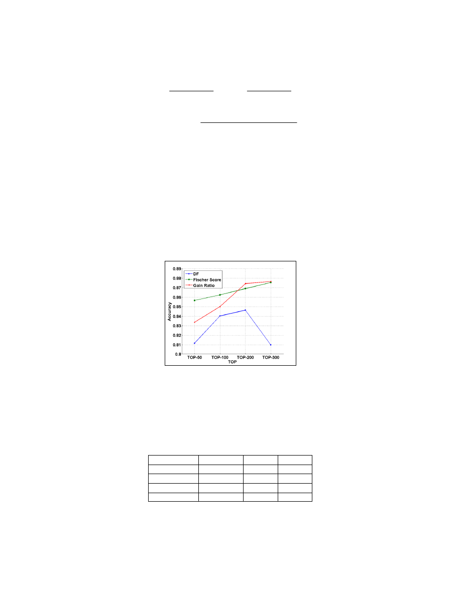
Feature Selections and Top Selections. Figure 1 presents the mean accuracy of the three feature
selections and the four top selections. Generally, the Fisher score was the best method, starting with
high accuracy even with 50 features. Unlike the others, in which the 300 features out-performed, the
DF’s accuracy decreased after the selection of more than 200 features, while the GR accuracy
significantly increased as more features were added.

Figure 1. The FS lead to very good results even with just 50 features and increased as the number of
features increased. At 200 features, the accuracy of GR increased significantly and the accuracy of
DF decreased.

In Table 1, we present the results of each classifier under the conditions, in which the highest mean
performance observed for all the classifiers: top 300 features selected by Fisher score where each
feature is 5-gram represented by TF from the top 5500 features. The DT and ANN outperform and
have low false positive rates, while the SVM-LIN also performed very well. The poor performance of
the Naïve Bayes may be explained by the features independence assumption of the NB classifier.

Table 1: The DT and ANN out-performed, while maintaining low levels of false positives.

Classifier

Accuracy

FP

FN

ANN

0.941

0.033

0.134

DT

0.943

0.039

0.099

NB

0.697

0.382

0.069

SVM-LIN

0.921

0.033

0.214

3.2.2 Experiment 2 – The Imbalance Problem
In the second experiment we present our main contribution, which was never investigated before. In
this set of experiments, we used the top 300 features selected by Fisher Score where each feature is

5-gram represented by TF from the top 5500 features (selected from the entire n-grams based on the
DF measure). We created five levels of Malicious Files Percentage (MFP) in the training set (16.7,
33.4, 50, 66.7 and 83.4%). For example, when referring to 16.7%, we mean that 16.7% of the files in
the training set were malicious and 83.4% were benign. The test set represents the real-life situation,
while the training set represents the set-up of the classifier, which is controlled. While we assume that
a MFP above 30% (of the total files) is not a realistic proportion in real networks, but we examined
high rates in order to gain insights into the behavior of the classifiers in these situations. Our study
examined 17 levels of MFP (5, 7.5, 10, 12.5, 15, 20, 30, 40, 50, 60, 70, 80, 85, 87.5, 90, 92.5 and
95%) in the test set. Eventually, we ran all the product combinations of five training sets and 17 test
sets, for a total of 85 runs for each classifier. We created two sets of data sets in order to perform a 2-
fold cross validation-like evaluation to make the results more significant.

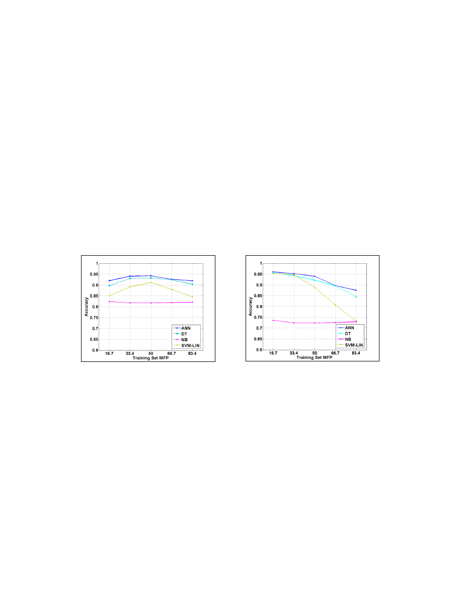
Training-Set Malcode Percentage. Figure 2 presents the mean accuracy (for all the MFP levels in
the test-sets) of each classifier for each training MFP level. The ANN and DT had the most accurate,
and relatively stable, performance across the different MFP levels in the training set, SVM-LIN
performed well, but not consistently, while NB generally performed poorly.

10% Malcode Percentage in the Test Set. We consider the 10% MFP level in the test set as a
realistic scenario. Figure 3 presents the mean accuracy in the 2-fold cross validation of each classifier
for each malcode content level in the training set, with a fixed level of 10% MFP in the test set.
Accuracy levels above 95% were achieved when the training set had a MFP of 16.7%, while a rapid
decrease in accuracy was observed when the MFP in the training set was increased. Thus, the
optimal proportion of malicious files in a training set for practical purposes should be less than 30%
malicious files.

Figure 2. Mean accuracy for various MFPs in the
test set. ANN and DT out-performed, with
consistent accuracy, across the different malcode
content levels.

Figure 3. Detection accuracy for 10% Malcode in
the test set. Greater than 95% accuracy was
achieved for the scenario involving a low level
(16.7%) of malicious file content in the training
set.

3.2.3 Experiment 3 – Chronological Evaluation
In this experiment we wanted to evaluate the importance and need in updating the training set. The
question was how important it is to update the repository of malicious and benign files and whether in
specific years the files were more contributive to the accuracy, when introduced in the training set or
in the test set. In order to answer these questions we divided the entire test collection into years from
2000 to 2007, in which the files were created. We had 7 training sets, in which each file contained
files from 2000 to 2006 (according to the year). Each training set was evaluated separately on each
following year till 2007. Additional we had two experimental setups, in which the training set had
16.6% MFP and 50% MFP, while the MFP at the test was set to 10% representing real life conditions.
We present the results of the chronological evaluation when we used the ANN classifier which
outperformed in the previous experiments.
Figure 4 presents the results when having 50% MFP at the training set. Generally, at most of the
cases the accuracy was between 0.9, out of when using the 2000 training set and when testing on
2006 and 2007. When testing on 2007 examples a decrease in the accuracy was observed, while
when the training set of till 2006 was used the highest accuracy was achieved.

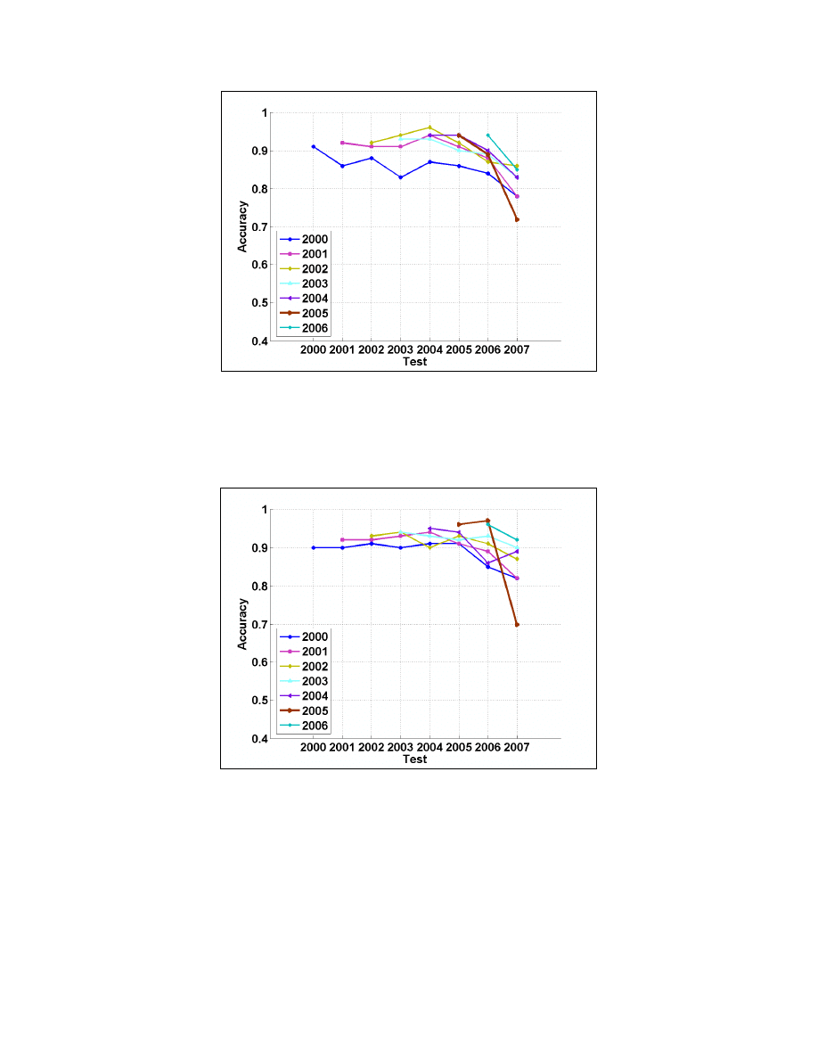
Figure 4. The results for having 50% MFP at the training set and 10% MFP at the test set. A

decrease in the performance is observed at the 2007 test set.

Figure 5 presents the results when 16.6% MFP was in the training set. Generally the accuracy was
higher, as expected, and there is a quite clear trend, in which as the training set is more updated the
accuracy is higher, out of the training set of till 2005 which had bad performance when testing on
2007.

Figure 5. The results for having 16.6% MFP at the training set and 10% MFP at the test set. A

decrease in the performance is observed at the 2007 test set.

4 Discussion and Conclusions
We presented a methodology for the representation of malicious and benign executables for the task
of unknown malicious code detection. This methodology enables the highly accurate detection of
unknown malicious code, based on previously seen other examples, while maintaining low levels of
false alarms. In order to reduce the number of n-gram features, which ranges from millions to billions,
we first used the DF measure to select the top 5500 features. Based on experiment 1, the Fisher
Score feature selection outperformed the other methods and using the top 300 features resulted in
the best performance. Generally, the ANN and DT achieved high mean accuracies, exceeding 94%,
with low levels of false alarms.

In the second experiment, we examined the relationship between the MFP in the test set, which
represents real-life scenario, and in the training-set, which being used for training the classifier. In this
experiment, we found that there are classifiers which are relatively inert to changes in the MFP level
of the test set. In general, the best mean performance (across all levels of MFP) was associated with
a 50% MFP in the training set (Fig. 2). However, when setting a level of 10% MFP in the test-set, as a
real-life situation, we looked at the performance of each level of MFP in the training set. A high level
of accuracy (above 95%) was achieved when less than 33% of the files in the training set were
malicious, while for specific classifiers, the accuracy was poor at all MFP levels (Fig. 3).
In the third experiment we wanted to learn the importance in updating the training set along the time.
Thus, we divided the test collection into years and evaluated training sets of selected years on the
next years. For 16% MFP in the training set and 10% MFP in the test set we found that the accuracy
was high most of the time, while in 2007 it slightly decreased. As was presented in the second
experiment 16.6% MFP in the training set was better.
Based on our extensive and rigorous experiments, we conclude that when one sets up a classifier for
use in a real-life situation, he should consider the expected proportion of malicious files in the stream
of data. Since we assume that, in most real-life scenarios, low levels of malicious files are present,
training sets should be designed accordingly. As future work we plan to apply this method on a dated
test collection, in which each file has its initiation date, to evaluate the real capability to detect
unknown malcode, based on previous known malcodes.

References

Abou-Assaleh, T., Cercone, N., Keselj, V., and Sweidan, R., N-gram Based Detection of New
Malicious Code, Proceedings of the 28th Annual International Computer Software and Applications
Conference, (2004).
Bishop, C., Neural Networks for Pattern Recognition. Clarendon Press, Oxford (1995).
Chawla, N. V., Japkowicz, N., and Kotcz, A. (2004) Editorial: special issue on learning from
imbalanced data sets. SIGKDD Explorations Newsletter 6(1):1-6.
Domingos, P., and Pazzani, M. (1997) On the optimality of simple Bayesian classifier under zero-one
loss, Machine Learning, 29:103-130.
Freund, Y., and Schapire, R.E. (1997) Decision-theoretic generalization of on-line learning and an
application to boosting, Journal of Computer and System Sciences, vol. 55, no. 1, pp. 119–139.
Gryaznov, D. Scanners of the Year 2000: Heuritics, Proceedings of the 5th International Virus
Bulletin, 1999.
Golub, T., Slonim, D., Tamaya, P., Huard, C., Gaasenbeek, M., Mesirov, J., Coller, H., Loh, M.,
Downing, J., Caligiuri, M., Bloomfield, C., and E. Lander, E. (1999) Molecular classification of cancer:
Class discovery and class prediction by gene expression monitoring, Science, 286:531-537.
Henchiri, O. and Japkowicz, N., A Feature Selection and Evaluation Scheme for Computer Virus
Detection. Proceedings of ICDM-2006: 891-895, Hong Kong, 2006.
Kolter, J.Z. and Maloof, M.A. (2004). Learning to detect malicious executables in the wild, in
Proceedings of the Tenth ACM SIGKDD International Conference on Knowledge Discovery and Data
Mining, 470–478. New York, NY: ACM Press.
Kolter J., and Maloof M., Learning to Detect and Classify Malicious Executables in the Wild, Journal of
Machine Learning Research, 7, 2721-2744, (2006).
Mitchell T. (1997) Machine Learning, McGraw-Hill.
Quinlan, J.R. (1993) C4.5: programs for machine learning. Morgan Kaufmann Publishers, Inc., San
Francisco, CA, USA.
Schultz, M., Eskin, E., Zadok, E., and Stolfo, S. (2001) Data mining methods for detection of new
malicious executables, in Proceedings of the IEEE Symposium on Security and Privacy, 2001, pp.
178-184.
Salton, G., Wong, A., and Yang, C.S. (1975) A vector space model for automatic indexing,
Communications of the ACM, 18:613-620.
Witten, I.H., and Frank, E. (2005) Data Mining: Practical machine learning tools and techniques, 2nd
Edition, Morgan Kaufmann Publishers, Inc., San Francisco, CA, USA.
S. Shin, J. Jung, H. Balakrishnan, Malware Prevalence in the KaZaA File-Sharing Network, Internet
Measurement Conference (IMC), Brazil, October 2006.

Robert Moskovitch is a PhD student at the Deutsche Telekom Laboratories at
Ben Gurion University, Israel. He has been working on several research
domains focusing on information retrieval, text categorization, machine learning
in security systems and data mining in general.

Deutsche Telekom Laboratories at Ben Gurion University
Robert Moskovitch
POB 653, Beer Sheva 84105, Israel
[phone] (Tel)
[phone]

(Fax)

[phone] (Mobile)
e-mail:

[e-mail]

www.bgu.ac.il/t-laboratories

Yuval Elovici is a senior lecturer at the Department of Information Systems
Engineering, Ben-Gurion University. He holds B.Sc. and M.Sc. degrees in
Computer and Electrical Engineering from the Ben-Gurion University of the
Negev, and a Ph.D. in Information Systems from Tel-Aviv University. His main
research interests are Computer and Network Security, Information Warfare,
Machine Learning and Information Retrieval. Currently he is the director of the
Deutsche Telekom Laboratories at Ben-Gurion University.

Deutsche Telekom Laboratories at Ben Gurion University
Dr. Yuval Elovici
Director
POB 653, Beer Sheva 84105, Israel
[phone] (Tel)
[phone]

(Fax)

[phone] (Mobile)
e-mail:

[e-mail]

www.bgu.ac.il/t-laboratories

www.ise.bgu.ac.il/faculty/elovici/