APPLIED OPTICS AND OPTICAL ENGINEERING, VOL. Xl

CHAPTER 1

Basic Wavefront Aberration Theory

for Optical Metrology

JAMES C. WYANT

Optical Sciences Center, University of Arizona

and

WYKO Corporation, Tucson, Arizona

KATHERINE CREATH

Optical Sciences Center

University of Arizona, Tucson, Arizona

I.

II.

III.

IV.

V.

VI.

VII.

VIII.

IX.

X.

XI.

XII.

Sign Conventions
Aberration-Free Image
Spherical Wavefront, Defocus, and Lateral Shift
Angular, Transverse, and Longitudinal Aberration
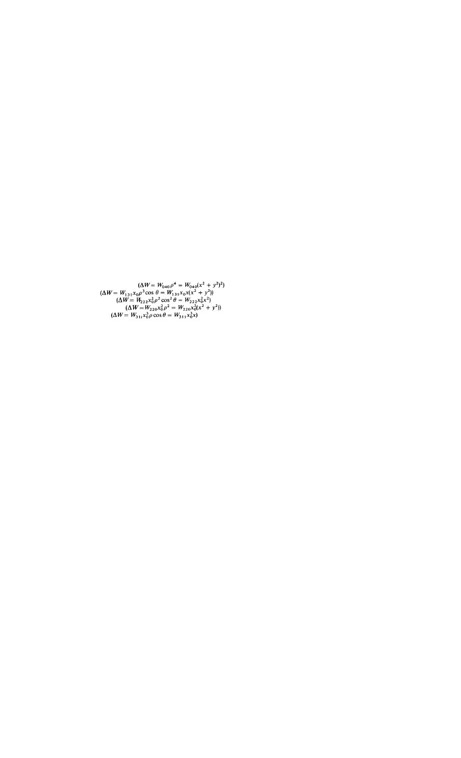
Seidel Aberrations
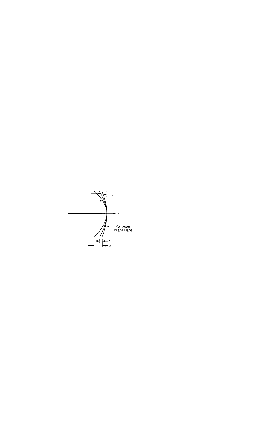
A. Spherical Aberration
B. Coma
C. Astigmatism
D. Field Curvature
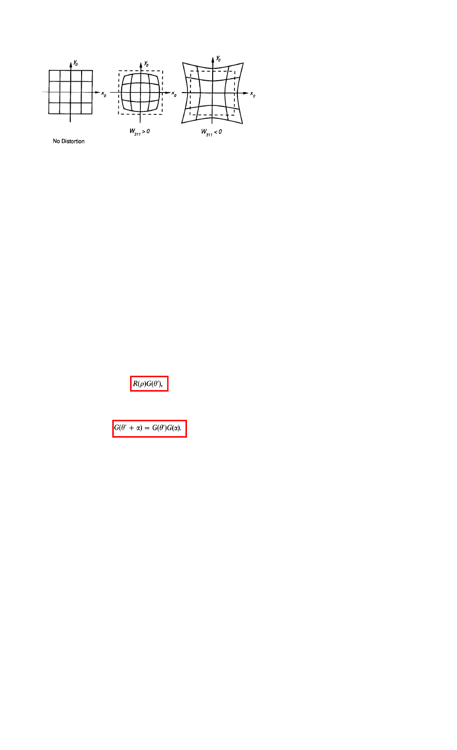
E. Distortion
Zernike Polynomials
Relationship between Zernike Polynomials and Third-Order
Aberrations
Peak-to-Valley and RMS Wavefront Aberration
Strehl Ratio
Chromatic Aberrations

Aberrations Introduced by Plane Parallel Plates
Aberrations of Simple Thin Lenses

2
4
9

12
15
18

22
24
26
28
28

35
36
38

40
40
46

XIII. Conics 48

A. Basic Properties

48

B. Spherical Aberration

50

C. Coma 51
D. Astigmatism 52

XIV. General Aspheres

52

References 53

1

Copyright © 1992 by Academic Press, Inc.

All rights of reproduction in any form reserved.

ISBN 0-12-408611-X

28

JAMES C. WYANT AND KATHERINE CREATH

VI. ZERNIKE POLYNOMIALS

Often, to aid in the interpretation of optical test results it is convenient to

express wavefront data in polynomial form. Zernike polynomials are often

Sagittal Focal Surface

Petzval Surface

Tangential Focal Surface

F

IG

.

33. Focal surfaces in presence of field curvature and astigmatism.

1. BASIC WAVEFRONT ABERRATION THEORY

29

Barrel Distortion

F

IG

. 34. Distortion,

Pincushion Distortion

used for this purpose since they are made up of terms that are of the

same

form as the types of aberrations often observed in optical tests

(Zernike,

1934). This is not to say that Zernike polynomials are the best polynomials

for fitting test data. Sometimes Zernike polynomials give a terrible represen-
tation of the wavefront data. For example, Zernikes have little value when air
turbulence is present. Likewise, fabrication errors present in the single-point
diamond turning process cannot be represented using a reasonable number
of terms in the Zernike polynomial. In the testing of conical optical elements,
additional terms must be added to Zernike polynomials to accurately
represent alignment errors. Thus,

the reader should be warned that the blind

use of Zernike polynomials to represent test results can lead to disastrous
results.

Zernike polynomials have several interesting properties. First, they are

one of an infinite number of complete sets of polynomials in two real
variables,

ρ

and

θ′

that are orthogonal in a continuous fashion over the

interior of a unit circle. It is important to note that the

Zernikes are

orthogonal only in a continuous fashion over the interior of a unit circle, and
in general they will not be orthogonal over a discrete set of data points within
a unit circle.

Zernike polynomials have three properties that distinguish them from

other sets of orthogonal polynomials. First, they have simple rotational
symmetry properties that lead to a polynomial product of the form

(49)

where G

(θ′

)

is a continuous function that repeats itself every 2

π

radians and

satisfies the requirement that rotating the coordinate system by an angle

α

does not change the form of the polynomial. That is,

(50)

30

JAMES C. WYANT AND KATHERINE CREATH

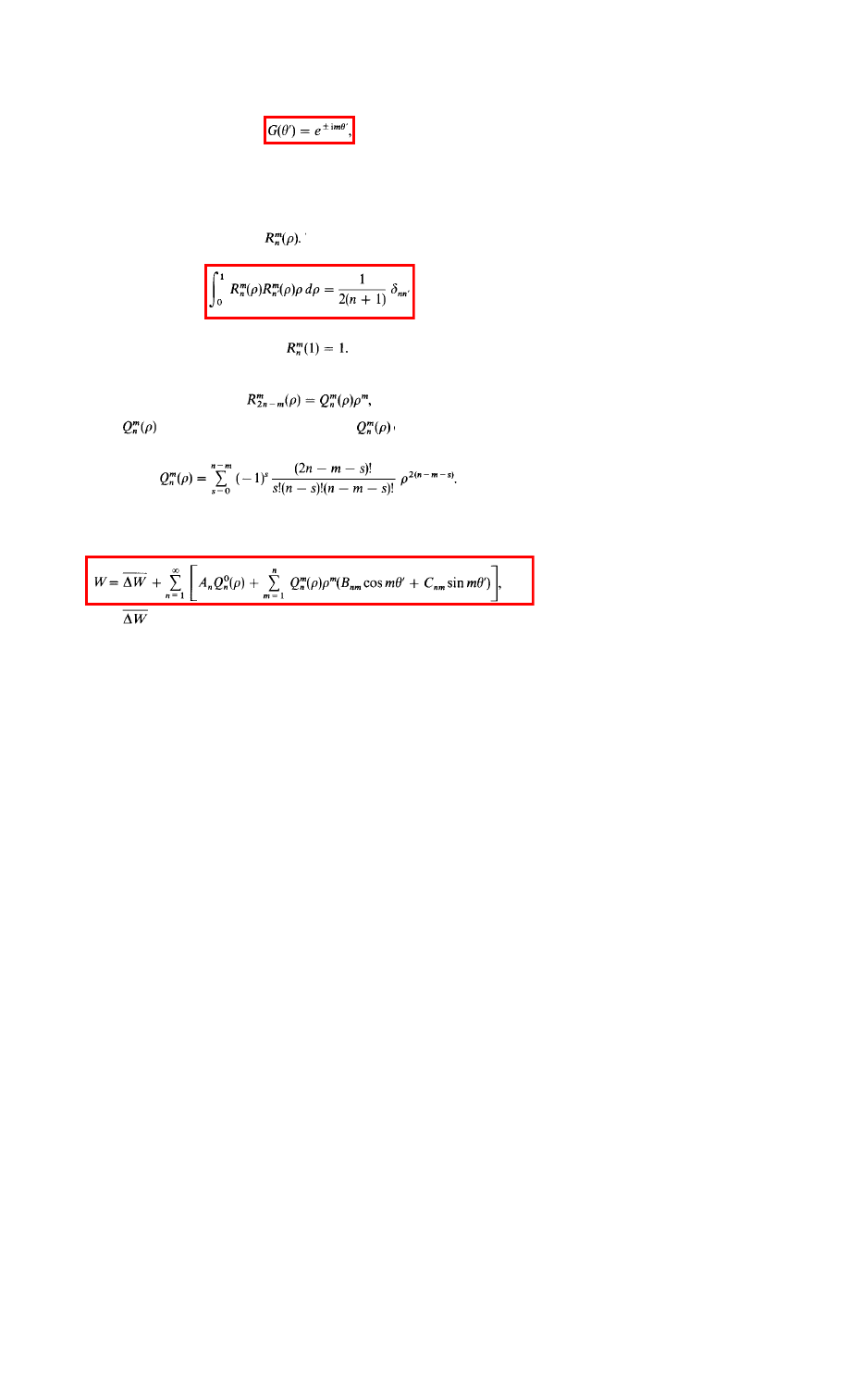
The set of trigonometric functions

(51)

where m is any positive integer or zero, meets these requirements.

The second property of Zernike polynomials is that the radial function

must be a polynomial in

ρ

of degree

n

and contain no power of

ρ

less than

m.

The third property is that R(p) must be even if

m

is even, and odd if

m

is odd.

The radial polynomials can be derived as a special case of Jacobi

polynomials, and tabulated as Their orthogonality and normalization
properties are given by

(52)

and

(53)

It is convenient to factor the radial polynomial into

(54)

where is a polynomial of order

2(n

-

m).

can be written generally

as

(55)

In practice, the radial polynomials are combined with sines and cosines

rather than with a complex exponential. The final Zernike polynomial series
for the wavefront OPD

∆

W can be written as

(56)

where is the mean wavefront OPD, and A

n

, B

nm

, and C

nm

are individual

polynomial coefficients. For a symmetrical optical system, the wave aberra-
tions are symmetrical about the tangential plane and only even functions of

θ′

are allowed. In general, however, the wavefront is not symmetric, and both
sets of trigonometric terms are included.

Table III gives a list of 36 Zernike polynomials, plus the constant term.

(Note that the ordering of the polynomials in the list is not universally
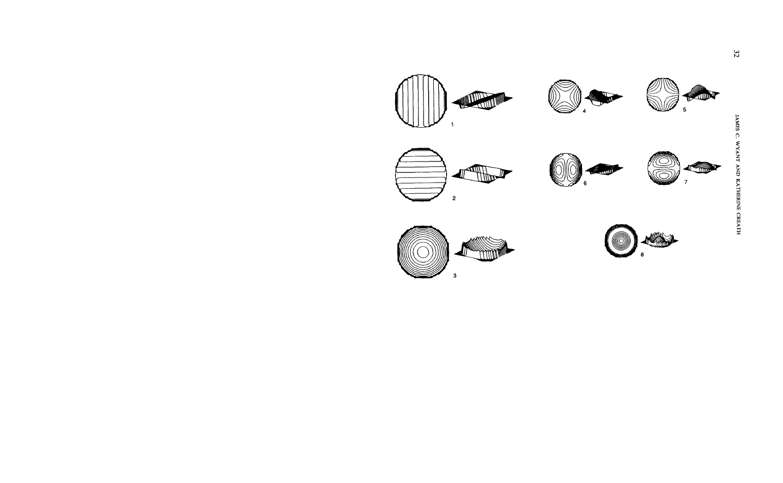
accepted, and different organizations may use a different ordering.) Figures 35
through 39 show contour maps of the 36 terms. Term #0 is a constant or
piston term, while terms # 1 and # 2 are tilt terms. Term # 3 represents focus.
Thus, terms # 1 through # 3 represent the Gaussian or paraxial properties of

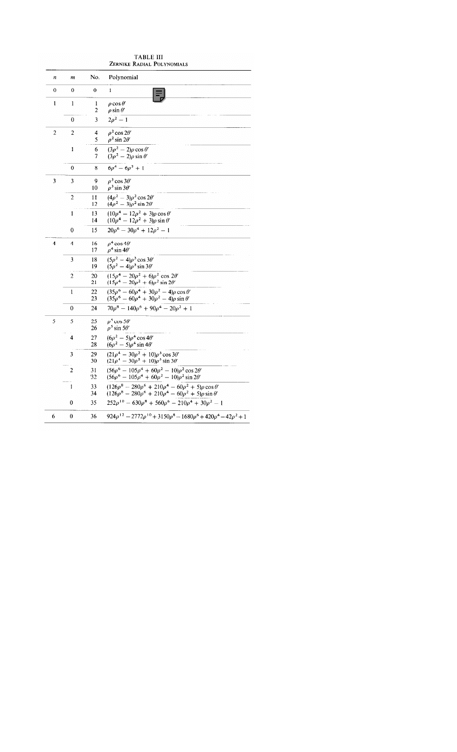
1. BASIC WAVEFRONT ABERRATION THEORY

31

n=1

FIRST-ORDER PROPERTIES

n=2

THIRD-ORDER ABERRATIONS

TILT

FOCUS

F

IG

. 35.

Two- and three-dimensional plots of Zernike poly-

nomials # 1 to # 3.

ASTIGMATISM AND DEFOCUS

COMA AND TILT

THIRD-ORDER SPHERICAL AND DEFOCUS

F

IG

. 36. Two- and three-dimensional plots of Zernike poly

nomials #4 to # 8.

FIFTH-ORDER

ABERRATIONS

ABERRATIONS

F

IG

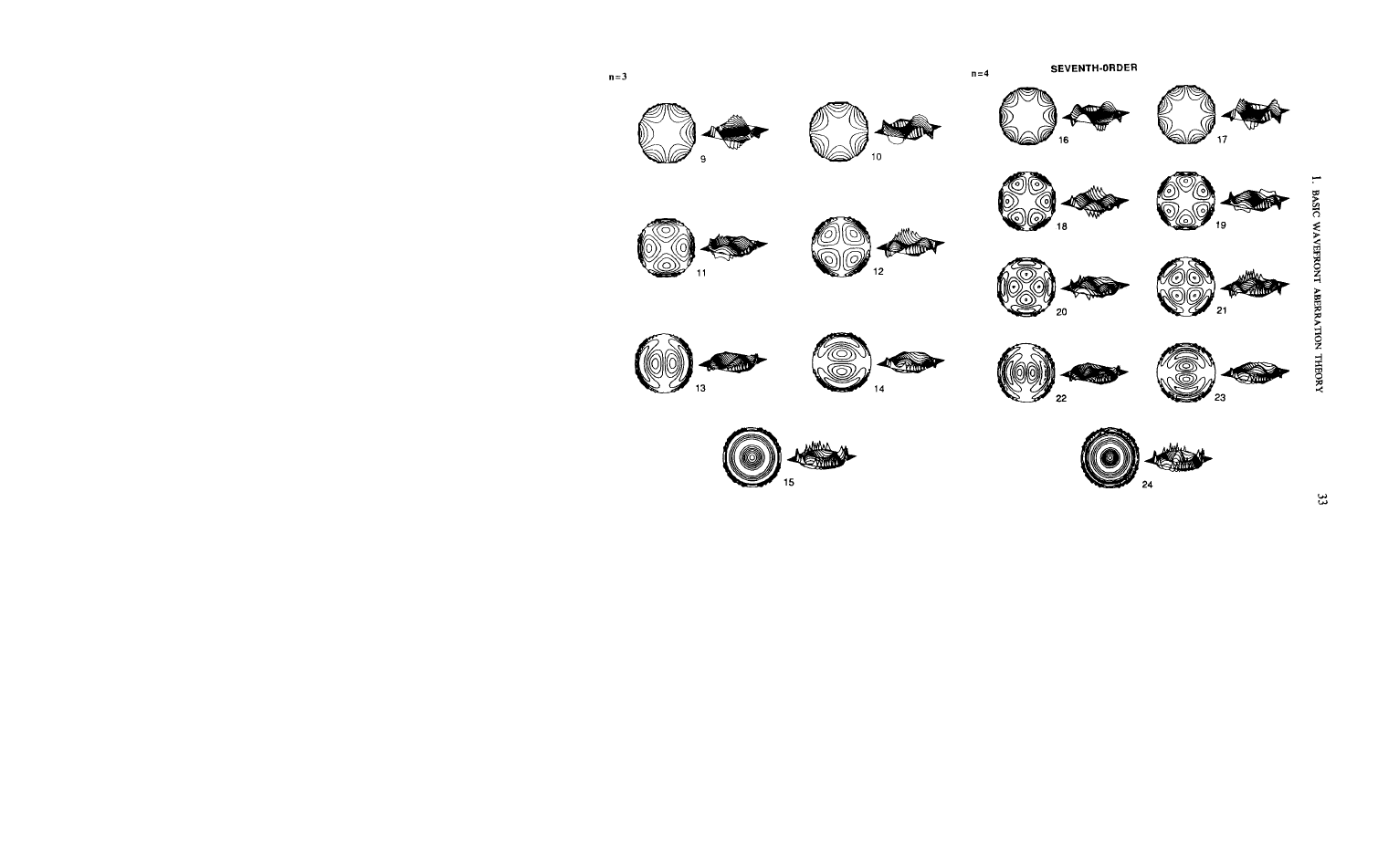
. 37. Two- and three-dimensional plots of Zernike poly-

nomials # 9 to # 15.

FIG. 38. Two- and three-dimensional plots of Zernike poly-

nomials # 16 to # 24.

34

JAMES C. WYANT AND KATHERINE CREATH

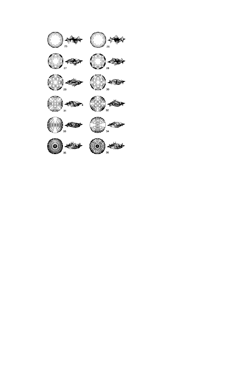
n=5,6

NINTH- & ELEVENTH-ORDER ABERRATIONS

F

IG

. 39. Two- and three-dimensional plots of Zernike polynomials # 25 to # 36.

the wavefront. Terms # 4 and # 5 are astigmatism plus defocus. Terms # 6
and #7 represent coma and tilt, while term #8 represents third-order
spherical and focus. Likewise, terms # 9 through # 15 represent fifth-order
aberration, # 16 through # 24 represent seventh-order aberrations, and # 25
through # 35 represent ninth-order aberrations.

Each term contains the

appropriate amount of each lower order term to make it orthogonal to each
lower order term. Also, each term of the Zernikes minimizes the rms
wavefront error to the order of that term. Adding other aberrations of lower
order can only increase the rms error. Furthermore, the average value of each
term over the unit circle is zero.

1. BASIC WAVEFRONT ABERRATION THEORY

35

VII. RELATIONSHIP BETWEEN ZERNIKE POLYNOMIALS AND

THIRD-ORDER ABERRATIONS

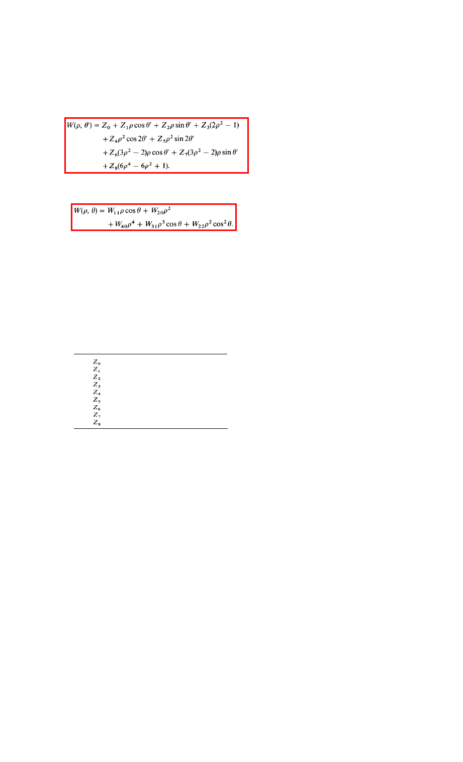
First-order wavefront properties and third-order wavefront aberration

coefficients can be obtained from the Zernike polynomials coefficients. Using
the first nine Zernike terms Z

0

to Z

8

, shown in Table III, the wavefront can

be written as

(57)

The aberrations and properties corresponding to these Zernike terms are
shown in Table IV. Writing the wavefront expansion in terms of field-
independent wavefront aberration coefficients, we obtain

(58)

Because there is no field dependence in these terms, they are not true Seidel
aberrations. Wavefront measurement using an interferometer only provides
data at a single field point. This causes field curvature to look like focus, and

distortion to look like tilt. Therefore, a number of field points must be
measured to determine the Seidel aberrations.

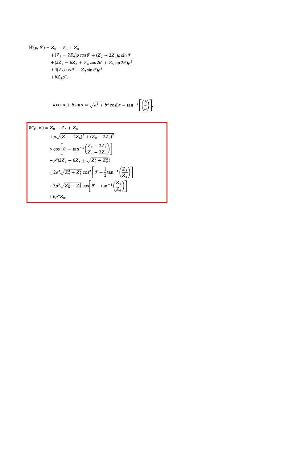
Rewriting the Zernike expansion of Eq. (57), first- and third-order field-

independent wavefront aberration terms are obtained. This is done by

TABLE IV

A

BERRATIONS

C

ORRESPONDING TO THE

F

IRST

N

INE

Z

ERNIKE

T

ERMS

piston
x-tilt
y-tilt
focus
astigmatism @ 0

o

& focus

astigmatism @ 45

o

& focus

coma & x-tilt
coma & y-tilt
spherical & focus

36

JAMES C. WYANT AND KATHERINE CREATH

grouping like terms, and equating them with the wavefront aberration
coefficients:

piston

tilt

focus + astigmatism

coma

spherical

(59)

Equation (59) can be rearranged using the identity

(60)

yielding terms corresponding to field-independent wavefront aberration
coefficients:

piston

tilt

focus

astigmatism

coma

spherical

(61)

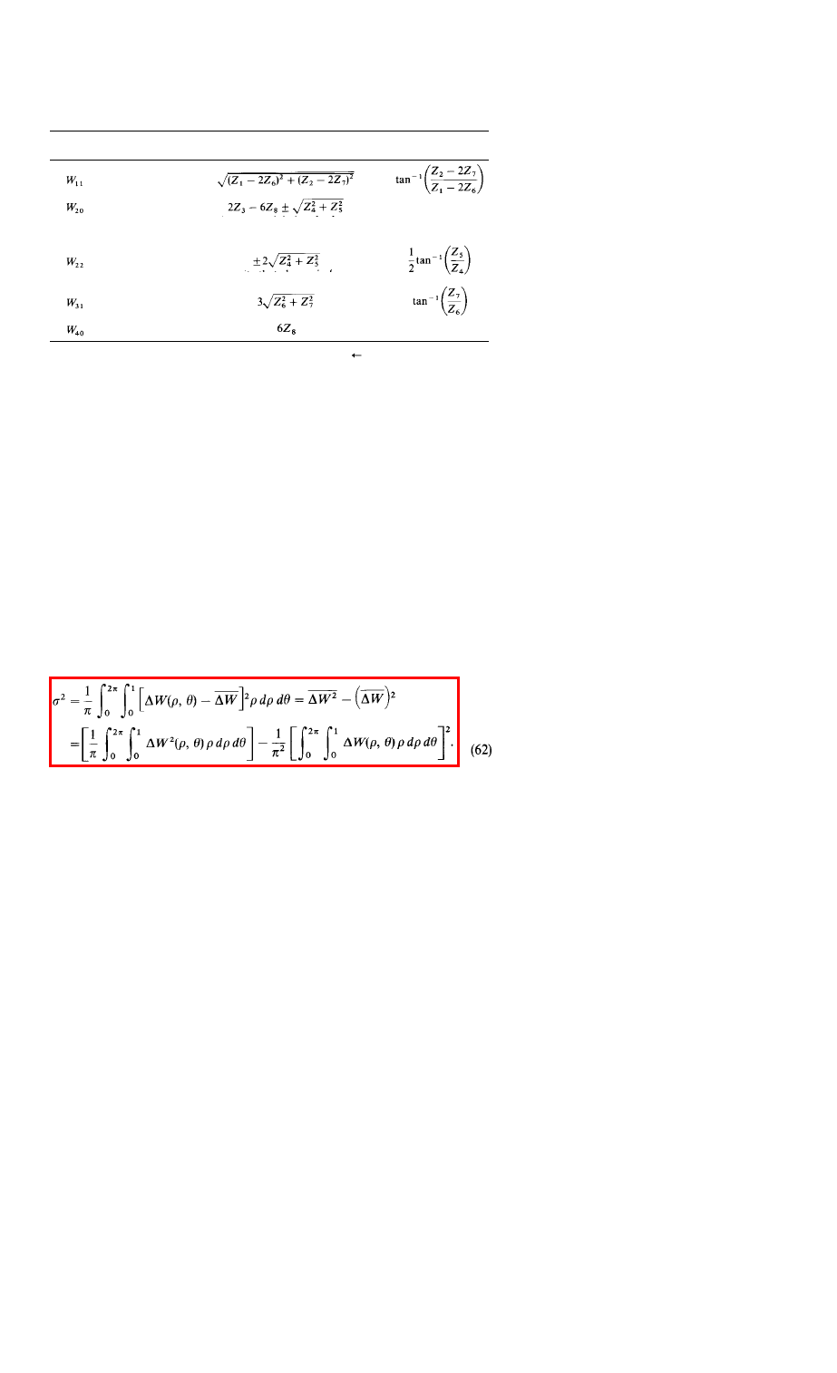
The magnitude, sign, and angle of these field-independent aberration terms
are listed in Table V. Note that focus has the sign chosen to minimize the
magnitude of the coefficient, and astigmatism uses the sign opposite that
chosen for focus.

VIII. PEAK-TO-VALLEY AND RMS WAVEFRONT ABERRATION

If the wavefront aberration can be described in terms of third-order

aberrations, it is convenient to specify the wavefront aberration by stating the
number of waves of each of the third-order aberrations present.

This method

1. BASIC WAVEFRONT ABERRATION THEORY

37

TABLE V

T

HIRD

-O

RDER

A

BERRATIONS IN

T

ERMS OF

Z

ERNIKE

C

OEFFICIENTS

Term Description

tilt

focus

Magnitude

sign chosen to minimize absolute value

of magnitude

Angle

astigmatism

sign opposite that chosen in focus term

coma

spherical

Note: For angle calculations, if denominator < 0, then angle angle + 180

o

.

for specifying a wavefront is of particular convenience if only a single third-
order aberration is present. For more complicated wavefront aberrations it is
convenient to state the

peak-to-valley (P-V)

sometimes called peak-to-peak

(P-P) wavefront aberration. This is simply the maximum departure of the
actual wavefront from the desired wavefront in both positive and negative
directions. For example, if the maximum departure in the positive direction is

+0.2 waves and the maximum departure in the negative direction is -0.1

waves, then the P-V wavefront error is 0.3 waves.

While using P-V to specify wavefront error is convenient and simple, it

can be misleading. Stating P-V is simply stating the maximum wavefront
error, and it is telling nothing about the area over which this error is

occurring. An optical system having a large P-V error may actually perform
better than a system having a small P-V error.

It is generally more

meaningful to specify wavefront quality using the rms wavefront error.

Equation (62) defines the rms wavefront error

σ

for a circular pupil, as

well as the variance

σ

2

. ∆

W

(ρ, θ)

is measured relative to the best fit spherical

wave, and it generally has the units of waves.

∆

W is the mean wavefront

OPD.

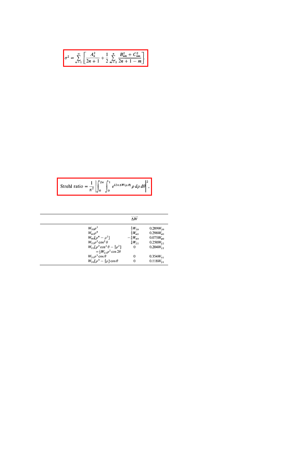
If the wavefront aberration can be expressed in terms of Zernike polynomials,

38

JAMES C. WYANT AND KATHERINE CREATH

the wavefront variance can be calculated in a simple form by using the
orthogonality relations of the Zernike polynomials. The final result for the

entire unit circle is

(63)

Table VI gives the relationship between

σ

and mean wavefront aberration for

the third-order aberrations of a circular pupil. While Eq. (62) could be used to
calculate the values of

σ

given in Table VI, it is easier to use linear

combinations of the Zernike polynomials to express the third-order aberra-
tions, and then use Eq. (63).

IX. STREHL RATIO

While

in the absence of aberrations, the intensity is a maximum at the

Gaussian image point.

If aberrations are present this will in general no longer

be the case.

The point of maximum intensity is called diffraction focus,

and for

small aberrations is obtained by finding the appropriate amount of tilt and

defocus to be added to the wavefront so that the wavefront variance is a
minimum.

The ratio of the intensity at the Gaussian image point (the origin of the

reference sphere is the point of maximum intensity in the observation plane)

in the presence of aberration, divided by the intensity that would be obtained
if no aberration were present, is called the Strehl ratio,

the Strehl definition,

or the Strehl intensity. The Strehl ratio is given by

TABLE VI

RELATIONSHIPS BETWEEN W

AVEFRONT

A

BERRATION

M

EAN AND RMS FOR

F

IELD

-I

NDEPENDENT

T

HIRD

-O

RDER

A

BERRATIONS

Aberration

∆

W

σ

Defocus
Spherical
Spherical & Defocus
Astigmatism
Astigmatism & Defocus

Coma
Coma & Tilt

(64)

1. BASIC WAVEFRONT ABERRATION THEORY

39

where

∆

W in units of waves is the wavefront aberration relative to the

reference sphere for diffraction focus. Equation (64) may be expressed in the
form

Strehl ratio =

(65)

If the aberrations are so small that the third-order and higher-order powers of
2

π

A W can be neglected, Eq. (65) may be written as

Strehl ratio

(66)

where

σ

is in units of waves.

Thus, when the aberrations are small, the Strehl ratio is independent of

the nature of the aberration and is smaller than the ideal value of unity by an
amount proportional to the variance of the wavefront deformation.

Equation (66) is valid for Strehl ratios as low as about 0.5. The Strehl ratio

is always somewhat larger than would be predicted by Eq. (66). A better
approximation for most types of aberration is given by

Strehl ratio

(67)

which is

good for Strehl ratios as small as 0.1.

Once the normalized intensity at diffraction focus has been determined,

the quality of the optical system may be ascertained using the Marécha1
criterion.

The Marécha1 criterion states that a system is regarded as well

corrected if the normalized intensity at diffraction focus is greater than or
equal to 0.8, which corresponds to an rms wavefront error

≤λ/14.

As mentioned in Section VI, a useful feature of Zernike polynomials is that

each term of the Zernikes minimizes the rms wavefront error to the order of
that term. That is, each term is structured such that adding other aberrations
of lower orders can only increase the rms error.

Removing the first-order

Zernike terms of tilt and defocus represents a shift in the focal point that
maximizes the intensity at that point. Likewise, higher order terms have built
into them the appropriate amount of tilt and defocus to minimize the rms

wavefront error to that order.

For example, looking at Zernike term 8 in

Table III shows that for each wave of third-order spherical aberration
present, one wave of defocus should be subtracted to minimize the rms
wavefront error and find diffraction focus.