

Excel 2002 Advanced Level
Table of Contents
Page
3
© MTC Training Solutions Ltd
Table of Contents
..........................................................................................18

Excel 2002 Advanced Level
Page
4
© MTC Training Solutions Ltd

Excel 2002 Advanced Level
Table of Contents
Page
5
© MTC Training Solutions Ltd


Excel 2002 Advanced Level
Introduction
Page
7
© MTC Training Solutions Ltd
Introduction
Excel ’2003 is a powerful spreadsheet application that allows users to produce tables
containing calculations and graphs. These can range from simple formulae through to
complex functions and mathematical models.
How to use this guide
This manual should be used as a point of reference following attendance of the advanced
level Excel ’2003 training course. It covers all the topics taught and aims to act as a
support aid for any tasks carried out by the user after the course.
The manual is divided into sections, each section covering an aspect of the introductory
course. The table of contents lists the page numbers of each section and the table of
figures indicates the pages containing tables and diagrams.
Objectives
Sections begin with a list of objectives each with its own check box so that you can mark
off those topics that you are familiar with following the training.
Instructions
Those who have already used a spreadsheet before may not need to read explanations on
what each command does, but would rather skip straight to the instructions to find out
how to do it. Look out for the hand icon
which precedes a list of instructions.
Appendices
The Appendices list the toolbars mentioned within the manual with a breakdown of their
functions and tables of shortcut keys.
Keyboard
Keys are referred to throughout the manual in the following way:
[ENTER] – denotes the return or enter key, [DELETE] – denotes the Delete key and so
on.
Where a command requires two keys to be pressed, the manual displays this as follows:

Excel 2002 Advanced Level
Introduction
Page
8
© MTC Training Solutions Ltd
[CTRL][P] – this means press the letter “p” while holding down the Control key.
Commands
When a command is referred to in the manual, the following distinctions have been made:
When menu commands are referred to, the manual will refer you to the menu bar –
E.g. “Choose File from the menu bar and then Print”.
When dialog box options are referred to, the following style has been used for the
text – “In the
Page Range
section of the Print dialog, click the
Current Page
option”
Dialog box buttons are shaded and boxed – “Click OK to close the Print dialog and
launch the print.”
Notes
Within each section, any items that need further explanation or extra attention devoted to
them are denoted by shading. For example:
“Excel will not let you close a document that you haven’t already saved
changes to without prompting you to save.”
Tips
At the end of each section there is a page for you to make notes on and a “Useful
Information” heading where you will find tips and tricks relating to the topics described
within the section.

Excel 2002 Advanced Level
Using advanced Worksheet functions
Page
9
© MTC Training Solutions Ltd
Section 1
Using advanced Worksheet functions
Objectives
By the end of this section you will be able to:
Create and use names in workbooks
Understand and use conditional formulae
Set up lookup tables and use LOOKUP
functions
Use the Goal Seek
Use the Solver
Excel 2002 Advanced Level
Using advanced Worksheet functions
Page
10
Names
When entering formulae or referring to any area on the spreadsheet, it is usual to refer to a
"range". For example, B6 is a range reference; B6:B10 is also a range reference. A
problem with this sort of reference is that it is not always easy to remember what cells to
reference. It may be necessary to write down the range, or select it, which often means
wasting time scrolling around the spreadsheet. Instead, Excel offers the chance to name
ranges on the spreadsheet, and to use these names to select cells, refer to them in formulae
or use them in Database, Chart or Macro commands.
Defining names
There are a number of ways to set up names on a spreadsheet. A common way is to use
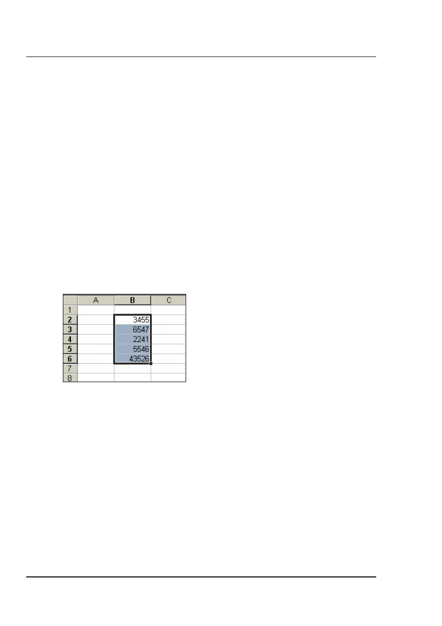
the Insert, Name, Define menu. In the example, there is a range of revenue figures that
could be named "REVENUE";
To name cells:
Mouse
1.
Select the cells you wish to name.
2.
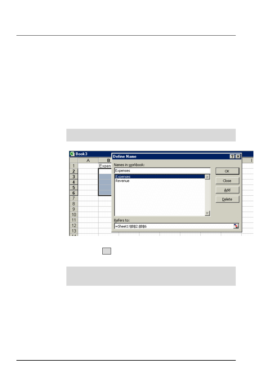
Choose Insert, Name, Define. The following dialog box appears;
© MTC Training Solutions Ltd

Excel 2002 Advanced Level
Using advanced Worksheet functions
Page
11
3.
The cursor flashes in the Names in workbook box, and below,
in the Refers to box, the range reference appears (notice that the
range is absolute).
4.
To name the cells, simply type a name in the Names in
workbook
box and choose OK.
A range can include any selection of cells, not necessarily a contiguous
row or column. Names can be up to 255 characters in length, must start
with a letter and cannot include spaces. Names are not case-sensitive.
In the example, these cells would be called REVENUE. From now on, any reference to
the range C3:C6 can be made with the name REVENUE. Notice that the name box, on
the left-hand side of the formula bar now displays the name REVENUE. It will do so
whenever cells C3:C6 are selected;
© MTC Training Solutions Ltd
Excel 2002 Advanced Level
Using advanced Worksheet functions
Page
12
Defining Names Automatically
Alternatively, cells can be named using text already on the spreadsheet. For instance, in a
spreadsheet, a column heading may have already been entered in cell C1 called
EXPENSES. This text can be used to name the cells below.
To define a name automatically:
Mouse
1.
Select cells C2:C6 and choose Insert, Name, Define.
The dialog box will automatically suggest the name EXPENSES because it
is entered in the cell above the selected cells;
2.
Choose OK and, again, the name appears in the Name box on the
formula bar.
This procedure works equally well with text entered to the left of a row of
data. For example, figures in cells B10:E10 can be named with the text in
cell A10;
Creating Names
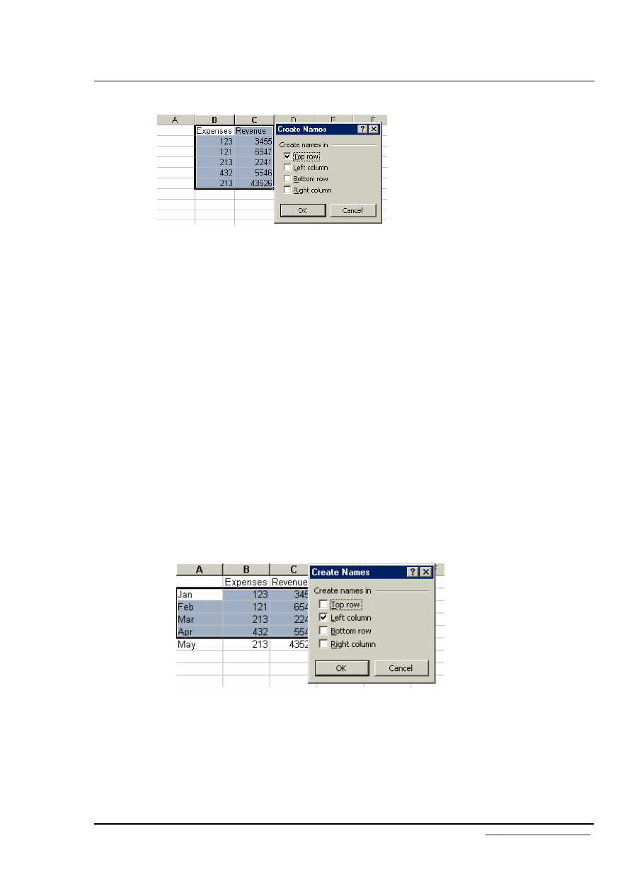
If appropriate names are already on the spreadsheet, Insert, Name, Create can be used as
an alternative to Define Name. This command is particularly useful for creating several
names at once;
© MTC Training Solutions Ltd
Excel 2002 Advanced Level
Using advanced Worksheet functions
Page
13
The above spreadsheet contains column headings to denote each month's figures. All
these figures could be named by the appropriate month using Insert, Name, Create. This
option requires not just the data to be selected, but the cells containing the names as well.
To create names:
Mouse
1.
Select cells B5:G8, and choose Insert, Name, Create. Excel will
automatically generate names in the top row of the selection, in
other words cells B6:B8 will be named JAN, C6:C8 FEB etc.
2.
To prove that these names have been created, choose Insert, Name,
Define, and the new names should be displayed.
The Create Names command can often lead to names intersecting each other. For
example, you may also want to name the rows of figures in the spreadsheet by their
respective countries;
Now the cells containing figures may form part of either the month name or the country
name. For instance, cell C6 is part of the range FEB, but also part of Britain. This cell can
actually be referred to using both names (in any order, separated by a space). Excel
knows that the name "FEB Britain" (or "Britain FEB") refers to the intersection point of
those two ranges, i.e. cell C6. These intersecting names can be used in formulae to refer
to specific cells (see later).
© MTC Training Solutions Ltd
Excel 2002 Advanced Level
Using advanced Worksheet functions
Page
14
USING NAMES
Goto
The GOTO feature can be used to go to a specific cell address on the spreadsheet. It can
also be used in conjunction with names.
To goto a name:
Mouse
1.
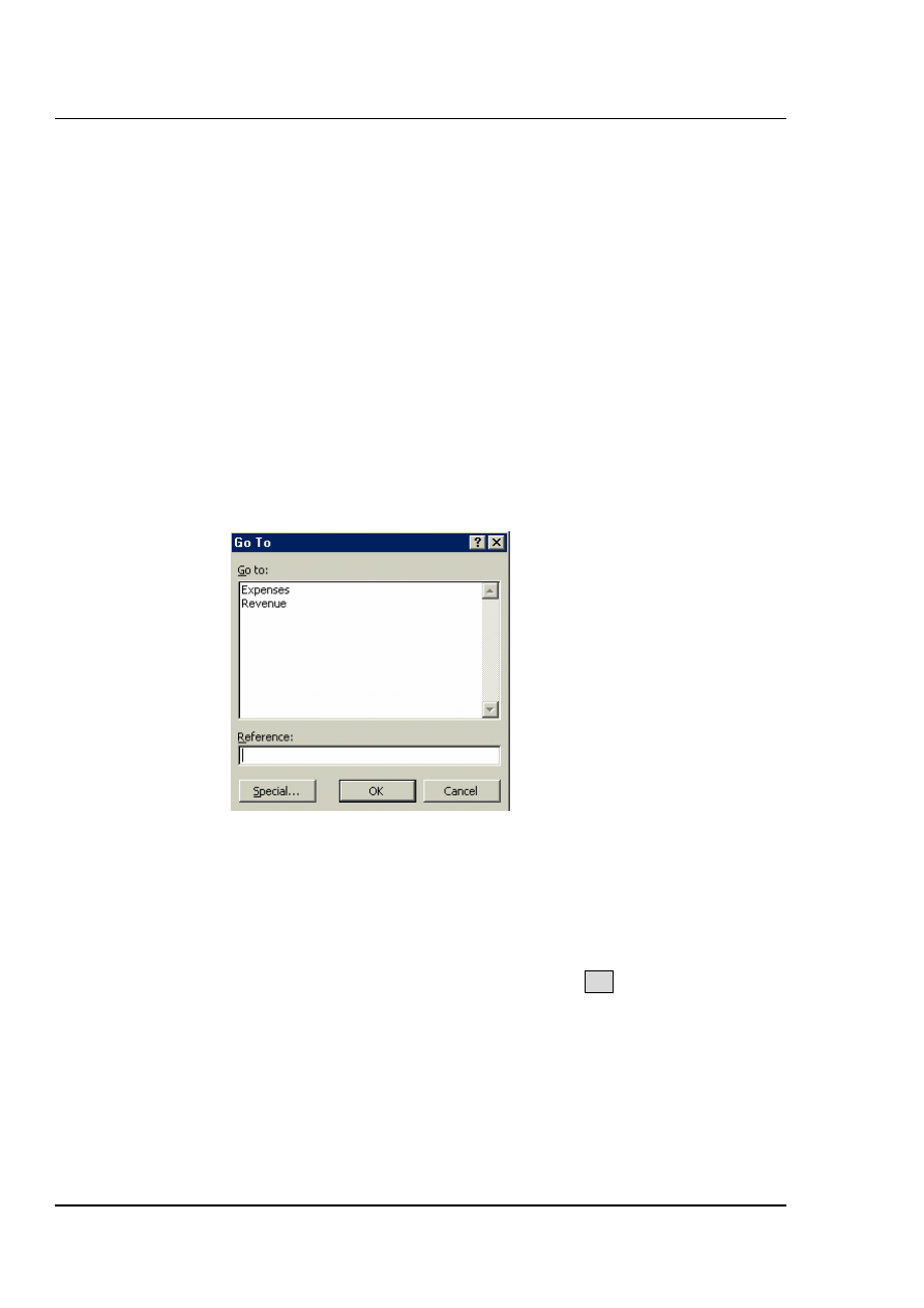
Choose Edit, Go To
Or
Keyboard
Press [F5]. The following dialog box appears;
2.
Click on the name required, then choose OK.
Not only does the cell pointer move to the correct range, but it also selects it. This can be
very useful for checking that ranges have been defined correctly, and also for listing all
the names on the spreadsheet.
You can also go to a specific cell that has been used in two range names. The previous
example mentioned cell C6, the intersection of the FEB and Britain ranges.
© MTC Training Solutions Ltd
Excel 2002 Advanced Level
Using advanced Worksheet functions
Page
15
To move to a cell that belongs to two ranges:
Keyboard
1.
Press [F5] and type the first range name in the Reference box,
then type a space and the second range name.
2.
Click OK. The pointer immediately jumps to the correct cell.
Names in Formulae
Names can be used in any simple formula, as well as any of Excel's built-in functions.
Instead of typing cell references or selecting cells, simply type the name or paste the
name into the formula.
=SUM(REVENUE)
=AVERAGE(INTEREST)
An intersecting name can be used, e.g.;
=France APR
=France APR + Germany MAY
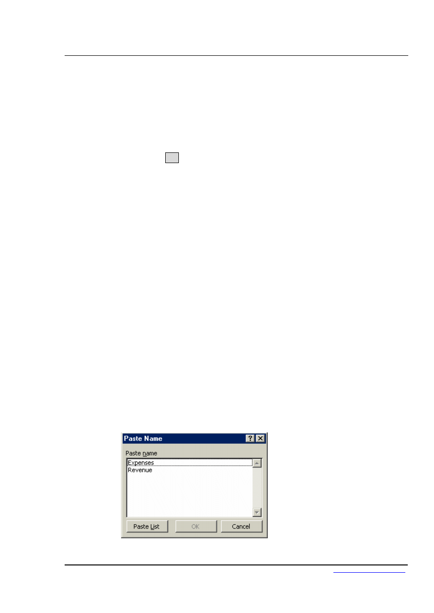
To avoid typing a name, choose from a list and paste in the required name.
To paste a name into a formula:
Mouse
1.
Choose Insert, Name, Paste.
© MTC Training Solutions Ltd
Excel 2002 Advanced Level
Using advanced Worksheet functions
Page
16
Or
Keyboard
Press [F3]
2.
Click on the required name and choose OK
To avoid typing altogether, choose Insert, Function, select the required
Category and Function, and click on OK. Then choose Insert, Name,
Paste, select the required name and click on OK. Then enter the formula.
Applying Names
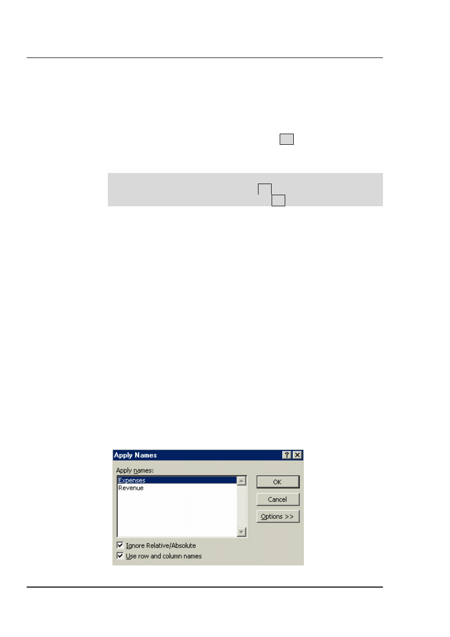
When a cell has already been referred to in a formula, and is then named, the name will
not automatically appear in the formula. Similarly, if a cell is referred to by its address
rather than its name, the name will not automatically appear. To replace all references
with names, the names must be applied.
Suppose a formula is written to sum cells B6:G6;
=SUM(B22:G22)
The formula makes no reference to the range "Britain", even though this range has been
named.
To replace cell references with range names:
Mouse
1.
Choose Insert, Name, Apply. The following dialog box appears;
© MTC Training Solutions Ltd

Excel 2002 Advanced Level
Using advanced Worksheet functions
Page
17
© MTC Training Solutions Ltd
2.
Click on the name you want, and choose OK.
To apply other names at the same time, use [Ctrl] and click on the
required names. The formula will now show the range names instead of
the cell references.
The Apply Names command works throughout the spreadsheet, so wherever the cell
reference to the name you chose appeared, the name is now in its place.

Excel 2002 Advanced Level
Using advanced Worksheet functions
Page
18
© MTC Training Solutions Ltd
Conditional & Logical Functions
Excel has a number of logical functions which allow you to set various "conditions" and
have data respond to them. For example, you may only want a certain calculation
performed or piece of text displayed if certain conditions are met. The functions used to
produce this type of analysis are found in the Insert, Function menu, under the heading
LOGICAL.
IF STATEMENTS
The IF function is used to analyse data, test whether or not it meets certain conditions and
then act upon its decision. The formula can be entered either by typing it or by pasting it
from the Formula, Paste Function box. Typically, the IF statement is accompanied by
three arguments enclosed in one set of parentheses; the condition to be met (logical_test);
the action to be performed if that condition is true (value_if_true); the action to be
performed if false (value_if_false). Each of these is separated by a comma, as shown;
=IF( logical_test , value_if_true , value_if_false)
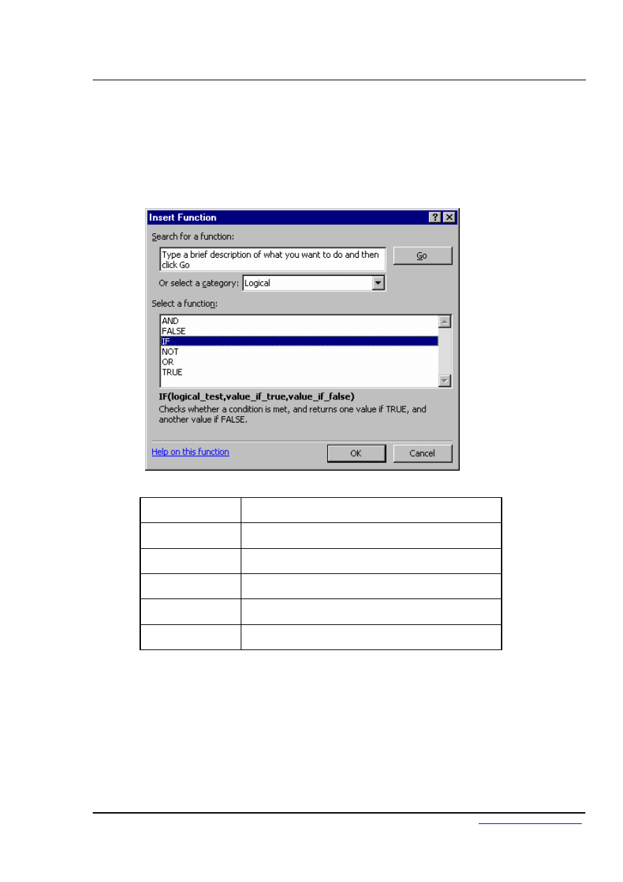
To view IF function syntax:
Mouse
1.
Click the Insert, Function menu.
2.
From the resulting dialog box, click on the LOGICAL category on
the left and the IF function on the right.
3.
The three arguments can be seen at the bottom of the screen;
Logical Test
Excel 2002 Advanced Level
Using advanced Worksheet functions
Page
19
This part of the IF statement is the "condition", or test. You may want to test to see if a
cell is a certain value, or to compare two cells. In these cases, symbols called LOGICAL
OPERATORS are useful;
>
greater than
<
less than
> =
greater than or equal to
< =
less than or equal to
=
equal to
< >
not equal to
Therefore, a typical logical test might be B1 > B2, testing whether or not the value
contained in cell B1 of the spreadsheet is greater than the value in cell B2. Names can
also be included in the logical test, so if cells B1 and B2 were respectively named SALES
and TARGET, the logical test would read SALES > TARGET. Another type of logical
test could include text strings. If you want to check a cell to see if it contains text, that
text string must be included in quotation marks. For example, cell C5 could be tested for
the word YES as follows; C5="YES".
© MTC Training Solutions Ltd
Excel 2002 Advanced Level
Using advanced Worksheet functions
Page
20
It should be noted that Excel's logic is, at times, brutally precise. In the above example,
the logical test is that sales should be greater than target. If sales are equal to target, the IF
statement will return the false value. To make the logical test more flexible, it would be
advisable to use the operator > = to indicate "meeting or exceeding".
Value if True / False
Provided that you remember that TRUE value always precedes FALSE value, these two
values can be almost anything. If desired, a simple number could be returned, a
calculation performed, or even a piece of text entered. Also, the type of data entered can
vary depending on whether it is a true or false result. You may want a calculation if the
logical test is true, but a message displayed if false. (Remember that text to be included in
functions should be enclosed in quotes).
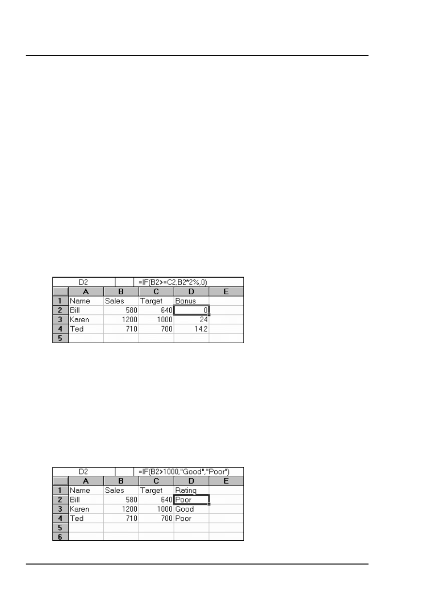
Taking the same logical test mentioned above, if the sales figure meets or exceeds the
target, a BONUS is calculated (e.g. 2% of sales). If not, no bonus is calculated so a value
of zero is returned. The IF statement in column D of the example reads as follows;
=IF(B2>=C2,B2*2%,0)
You may, alternatively, want to see a message saying "NO BONUS". In this case, the true
value will remain the same and the false value will be the text string "NO BONUS";
=IF(B2>=C2,B2*2%,"NO BONUS")
A particularly common use of IF statements is to produce "ratings" or "comments" on
figures in a spreadsheet. For this, both the true and false values are text strings. For
example, if a sales figure exceeds a certain amount, a rating of "GOOD" is returned,
otherwise the rating is "POOR";
=IF(B2>1000,"GOOD","POOR")
© MTC Training Solutions Ltd
Excel 2002 Advanced Level
Using advanced Worksheet functions
Page
21
NESTED IF
When you need to have more than one condition and more than two possible outcomes, a
NESTED IF is required. This is based on the same principle as a normal IF statement, but
involves "nesting" a secondary formula inside the main one. The secondary IF forms the
FALSE part of the main statement, as follows;
=IF(1st logic test , 1st true value , IF(2nd logic test , 2nd true value , false value))
Only if both logic tests are found to be false will the false value be returned. Notice that
there are two sets of parentheses, as there are two separate IF statements. This process can
be enlarged to include more conditions and more eventualities - up to seven IFs can be
nested within the main statement. However, care must be taken to ensure that the correct
number of parentheses are added.
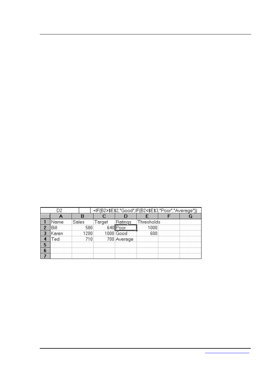
In the example, sales staff could now receive one of three possible ratings ;
=IF(B2>1000,"GOOD",IF(B2<600,"POOR","AVERAGE"))
To make the above IF statement more flexible, the logical tests could be amended to
measure sales against cell references instead of figures. In the example, column E has
been used to hold the upper and lower sales thresholds.
=IF(B2>$E$2,"GOOD",IF(B2<$E$3,"POOR","AVERAGE"))
(If the IF statement is to be copied later, this cell reference should be absolute).
© MTC Training Solutions Ltd
Excel 2002 Advanced Level
Using advanced Worksheet functions
Page
22
Statistical If Statements
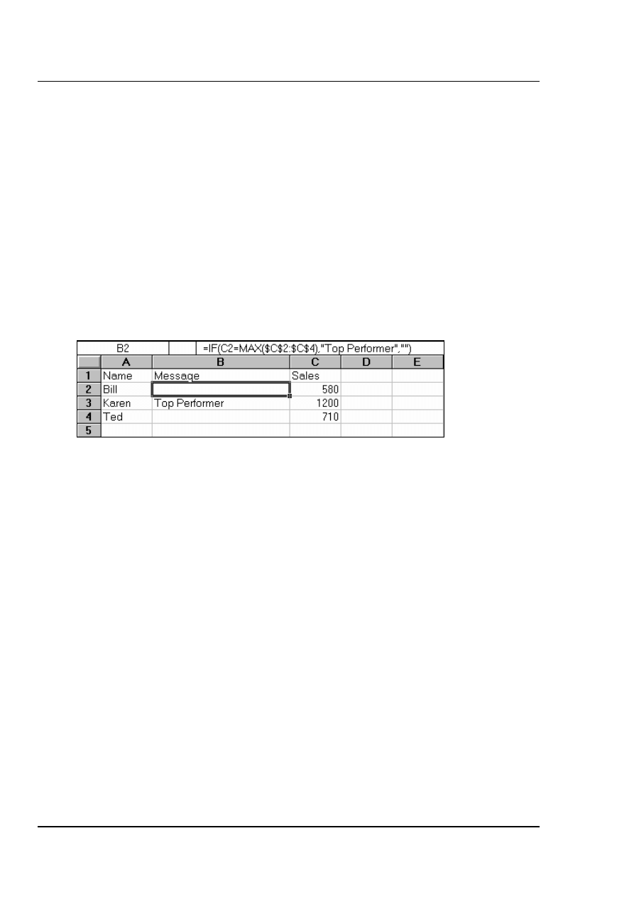
A very useful technique is to display text or perform calculations only if a cell is the
maximum or minimum of a range. In this case the logical test will contain a nested
statistical function (such as MAX or MIN). If, for example, a person's sales cell is the
maximum in the sales column, a message stating "Top Performer" could appear next to
his or her name. If the logical test is false, a blank message could appear by simply
including an empty set of quotation marks. When typing the logical test, it should be
understood that there are two types of cell referencing going on. The first is a reference to
one person's figure, and is therefore relative. The second reference represents the RANGE
of everyone's figures, and should therefore be absolute.
=IF(relative cell = MAX(absolute range) , "Top Performer" , "")
In this example the IF statement for cell B2 will read;
=IF(C2=MAX($C$2:$C$4),"Top Performer","")
When this is filled down through cells B3 and B4, the first reference to the individual's
sales figure changes, but the reference to all three sales figures ($C$2:$C$4) should
remain constant. By doing this, you ensure that the IF statement is always checking to see
if the individual's figure is the biggest out of the three.
A further possibility is to nest another IF statement to display a message if a value is the
minimum of a range. Beware of syntax here - the formula could become quite unwieldy!
© MTC Training Solutions Ltd
Excel 2002 Advanced Level
Using advanced Worksheet functions
Page
23
AND, OR, NOT
Rather than create large and unwieldy formulae involving multiple IF statements, the
AND, OR and NOT functions can be used to group logical tests or "conditions" together.
These three functions can be used on their own, but in that case they will only return the
values "TRUE" or "FALSE". As these two values are not particularly meaningful on a
spreadsheet, it is much more useful to combine the AND, OR and NOT functions within
an IF statement. This way, you can ask for calculations to be performed or other text
messages to appear as a result.
And
This function is a logical test to see if all conditions are true. If this is the case, the value
"TRUE" is returned. If any of the arguments in the AND statement are found to be false,
the whole statement produces the value "FALSE". This function is particularly useful as a
check to make sure that all conditions you set are met.
Arguments are entered in the AND statement in parentheses, separated by commas, and
there is a maximum of 30 arguments to one AND statement. The following example
checks that two cells, B1 and B2, are both greater than 100.
=AND(B1>100,B2>100)
If either one of these two cells contains a value less than a hundred, the result of the AND
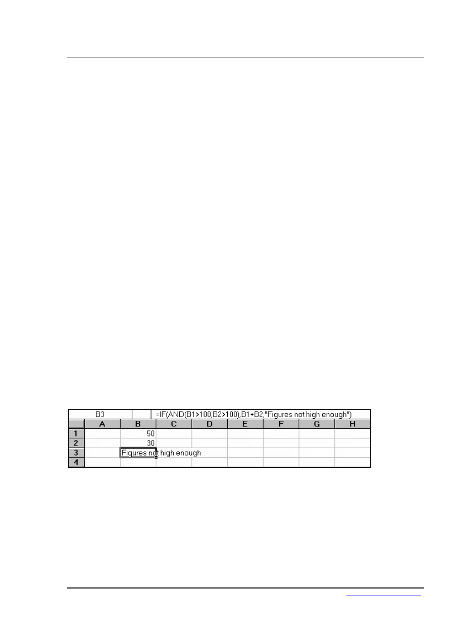
statement is "FALSE". This can now be wrapped inside an IF function to produce a more
meaningful result. You may want to add the two figures together if they are over 100, or
display a message indicating that they are not high enough.
=IF(AND(B1>100,B2>100),B1+B2,"Figures not high enough")
Another application of ANDs is to check that a number is between certain limits. The
following example checks that a number is between 50 and 100. If it is, the value is
entered. If not, a message is displayed;
=IF(AND(B1>50,B1<100),B1,"Number is out of range")
© MTC Training Solutions Ltd
Excel 2002 Advanced Level
Using advanced Worksheet functions
Page
24
Or
This function is a logical test to see if one or more conditions are true. If this is the case,
the value "TRUE" is returned. If just one of the arguments in the OR statement is found to
be true, the whole statement produces the value "TRUE". Only when all arguments are
false will the value "FALSE" be returned. This function is particularly useful as a check
to make sure that at least one of the conditions you set is met.
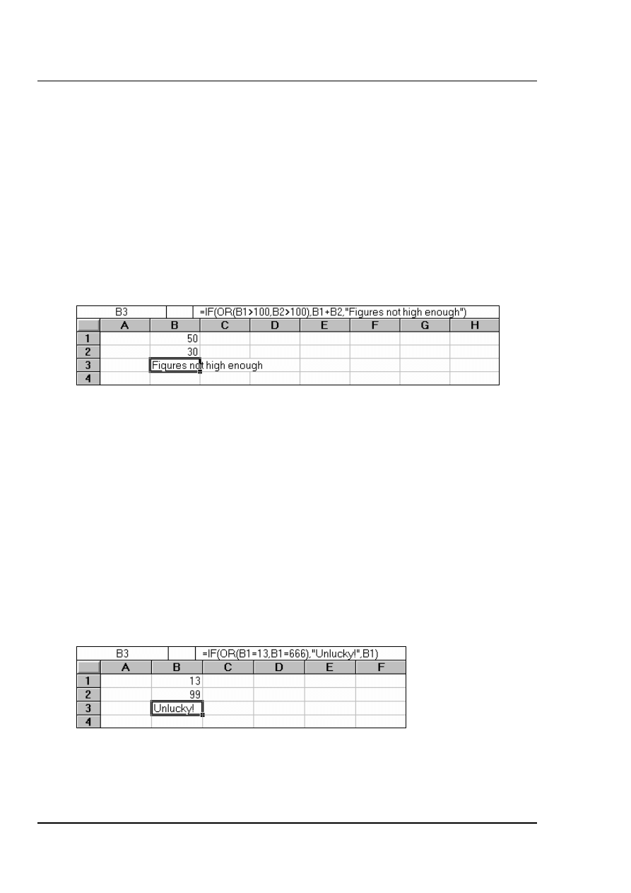
=IF(OR(B1>100,B2>100),B1+B2,"Figures not high enough")
In the above formula, only one of the numbers in cells B1 and B2 has to be over 100 in
order for them to be added together. The message only appears if neither figure is high
enough.
Not
NOT checks to see if the argument is false. If so, the value "TRUE" is returned. It is best
to use NOT as a "provided this is not the case" function. In other words, so long as the
argument is false, the overall statement is true. In the example, the cell contents of B1 is
returned unless the number 13 is encountered. If B1 is found to contain 13, the message
"Unlucky!" is displayed;
=IF(NOT(B1=13),B1,"Unlucky!")
The NOT function can only contain one argument. If it is necessary to check that more
than one argument is false, the OR function should be used and the true and false values
of the IF statement reversed. Suppose, for example, a check is done against the numbers
13 and 666;
=IF(OR(B1=13,B1=666),"Unlucky!",B1)
© MTC Training Solutions Ltd

Excel 2002 Advanced Level
Using advanced Worksheet functions
Page
25
© MTC Training Solutions Ltd
Lookup Functions
As already mentioned, Excel can produce varying results in a cell, depending on
conditions set by you. For example, if numbers are above or below certain limits,
different calculations will be performed and text messages displayed. The usual method
for constructing this sort of analysis is using the IF function. However, as already
demonstrated, this can become large and unwieldy when you want multiple conditions
and many possible outcomes. To begin with, Excel can only nest seven IF clauses in a
main IF statement, whereas you may want more than eight logical tests or "scenarios". To
achieve this, Excel provides some LOOKUP functions. These functions allow you to
create formulae which examine large amounts of data and find information which
matches or approximates to certain conditions. They are simpler to construct than nested
IFs and can produce many more varied results.
LOOKUP
Before you actually start to use the various LOOKUP functions, it is worth learning the
terms that you will come across, what they mean and the syntax of the function
arguments.
Vector Lookup
A vector is a series of data that only occupies one row or column. LOOKUP will look
through this row or column to find a specific value. When the value is found, a
corresponding "result" in the adjacent row or column is returned. For example, column D
of a spreadsheet may contain figures, and the adjacent column E contain corresponding
text. LOOKUP will search for the requested figure in column D and return the
corresponding text from column E.
The syntax for LOOKUP is as follows;
=LOOKUP( lookup_value , lookup_vector , result_vector )
The lookup_value represents the number or text entry to look for; the lookup_vector is the
area in which to search for the lookup_value; the result_vector is the adjacent row or
column where the corresponding value or text is to be found.
It is essential that data in the lookup vector is placed in ascending order,
i.e. numbers from lowest to highest, text from A to Z. If this is not done, the
LOOKUP function may return the wrong result.

Excel 2002 Advanced Level
Using advanced Worksheet functions
Page
26
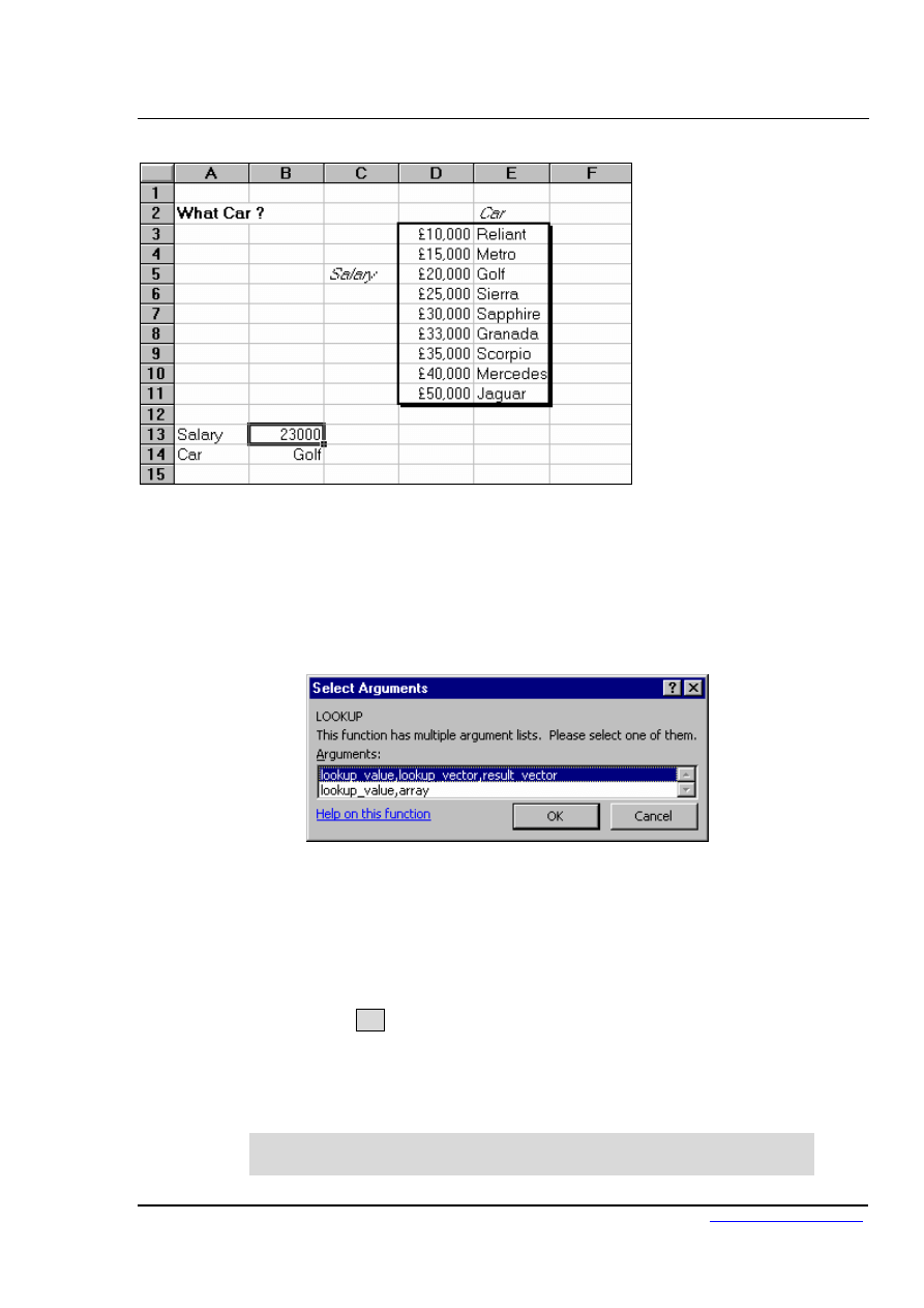
In the diagram, column D contains varying salaries, against which there is a company car
in column E which corresponds to each salary. For example, a £20030 salary gets a Golf,
a £35000 salary gets a Scorpio. A LOOKUP formula can be used to return whatever car is
appropriate to a salary figure that is entered. In this case, the lookup_value is the cell
where the salary is entered (B13), the lookup_vector is the salary column (D3:D11), and
the result_vector is the car column (E3:E11). Hence the formula;
=LOOKUP(B13,D3:D11,E3:E11)
Typing 40000 in cell B13 will set the lookup_value. LOOKUP will search through the
lookup_vector to find the matching salary, and return the appropriate car from the
result_vector, which in this case is Mercedes.
Alternatively, the formula could be simplified and cell references avoided by using
Formula, Define Name to give appropriate range names. Call B13 Salary, D3:D11
Salaries and E3:E11 Cars. The LOOKUP formula could then be simplified to;
=LOOKUP(Salary,Salaries,Cars)
One of the advantages of the LOOKUP function is that if the exact lookup_value is not
found, it will approximate to the nearest figure below the requested value. For instance, if
a user enters a Salary of 23000, there is no figure in the Salaries range which matches
this. However, the nearest salary below 23000 is 20030, so the corresponding car is
returned, which is a Golf. This technique is very useful when the lookup_vector indicates
grades or "bands". In this case, anyone in the salary "band" between 20030 and 25000
gets a Golf. Only when their salary meets or exceeds 25000 do they get a Sierra.
© MTC Training Solutions Ltd
Excel 2002 Advanced Level
Using advanced Worksheet functions
Page
27
There may be occasions where the lookup_value is below the lowest value in the vector.
In this case the #N/A message is displayed.
To insert a lookup function:
Mouse
1.
2.
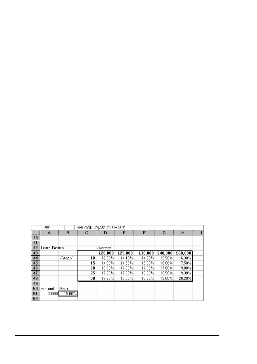
Use the Insert, Function menu and click on the LOOKUP &
REFERENCE category, then on the LOOKUP function on the
right.
When OK is chosen, another dialog box appears displaying the two
versions of LOOKUP. There are two syntax forms; the first is the
"array" and the second the "vector".
The second of these forms, the "vector" LOOKUP is by far the most useful,
and it is recommended that you only use this form.
© MTC Training Solutions Ltd
Excel 2002 Advanced Level
Using advanced Worksheet functions
Page
28
HLOOKUP
The horizontal LOOKUP function (HLOOKUP) can be used not just on a "vector" (single
column or row of data), but on an "array" (multiple rows and columns). HLOOKUP
searches for a specified value horizontally along the top row of an array. When the value
is found, HLOOKUP searches down to a specified row and enters the value of the cell.
This is useful when data is arranged in a large tabular format, and it would be difficult for
you to read across columns and then down to the appropriate cell. HLOOKUP will do this
automatically.
The syntax for HLOOKUP is;
=HLOOKUP( lookup_value , table_array , row_index_number)
The lookup_value is, as before, a number, text string or cell reference which is the value
to be found along the top row of the data; the table_array is the cell references (or range
name) of the entire table of data; the row_index_number represents the row from which
the result is required. This must be a number, e.g. 4 instructs HLOOKUP to extract a
value from row 4 of the table_array.
It is important to remember that data in the array must be in ascending order. With a
simple LOOKUP function, only one column or row of data, referred to as a vector, is
required. HLOOKUP uses an array (i.e. more than one column or row of data). Therefore,
as HLOOKUP searches horizontally (i.e. across the array), data in the first row must be in
ascending order, i.e. numbers from lowest to highest, text from A to Z. As with
LOOKUP, if this rule is ignored, HLOOKUP will return the wrong value.
As an example, a user may have a spreadsheet which displays various different rates of
interest for a range of amounts over different time periods;
© MTC Training Solutions Ltd

Excel 2002 Advanced Level
Using advanced Worksheet functions
Page
29
© MTC Training Solutions Ltd
Whatever the amount a customer wants to borrow, he may pay up to five different rates of
interest depending on whether the loan is over 10, 15 or more years. The HLOOKUP
function will find a specific amount, then move down the array to find the appropriate
interest rate for the required time period.
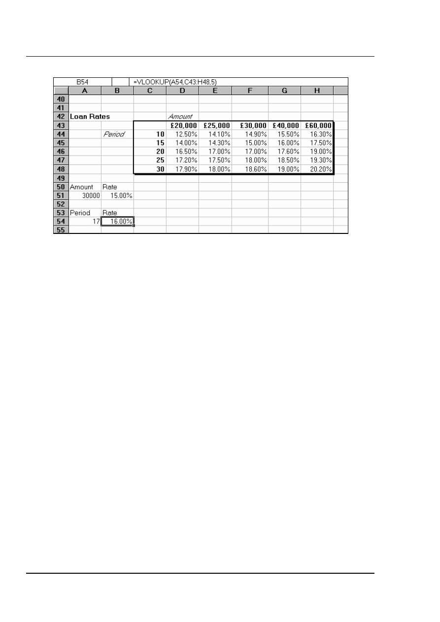
Designate cell A51 as the cell to hold the amount, i.e. the lookup_value; cells C43:H48
are the table_array; the row_index_number will be 2 if a customer wants the loan over 10
years, 3 if he wants the loan over 15 years, and so on. Cell B51 holds this formula;
=HLOOKUP(A51,C43:H48,3)
The above formula looks along the top row of the array for the value in cell A51 (30000).
It then moves down to row 3 and returns the value 15.00%, which is the correct interest
rate for a £30000 loan over 15 years. (Range names could be used here to simplify the
formula).
As with the LOOKUP function, the advantage of HLOOOKUP is that it does not
necessarily have to find the exact lookup_value. If, for example, you wanted to find out
what interest rate is applicable to a £28000 loan, the figure 28000 can be entered in the
lookup_value cell (A51) and the rate 14.30% appears. As before, Excel has looked for the
value in the array closest to, but lower than, the lookup_value.
VLOOKUP
The VLOOKUP function works on the same principle as HLOOKUP, but instead of
searching horizontally, VLOOKUP searches vertically. VLOOKUP searches for a
specified value vertically down the first column of an array. When the value is found,
VLOOKUP searches across to a specified column and enters the value of the cell. The
syntax for the VLOOKUP function follows the same pattern as HLOOKUP, except that
instead of specifying a row index number, you would specify a column index number to
instruct VLOOKUP to move across to a specific column in the array where the required
value is to be found.
=VLOOKUP( lookup_value , table_array , col_index_number )
In the case of VLOOKUP, data in the first column of the array should be in ascending
order, as VLOOKUP searches down this column for the lookup_value.
In the same spreadsheet as before, a VLOOKUP formula could be used to search for a
specific time period, then return the appropriate rate for a fixed amount. In the following
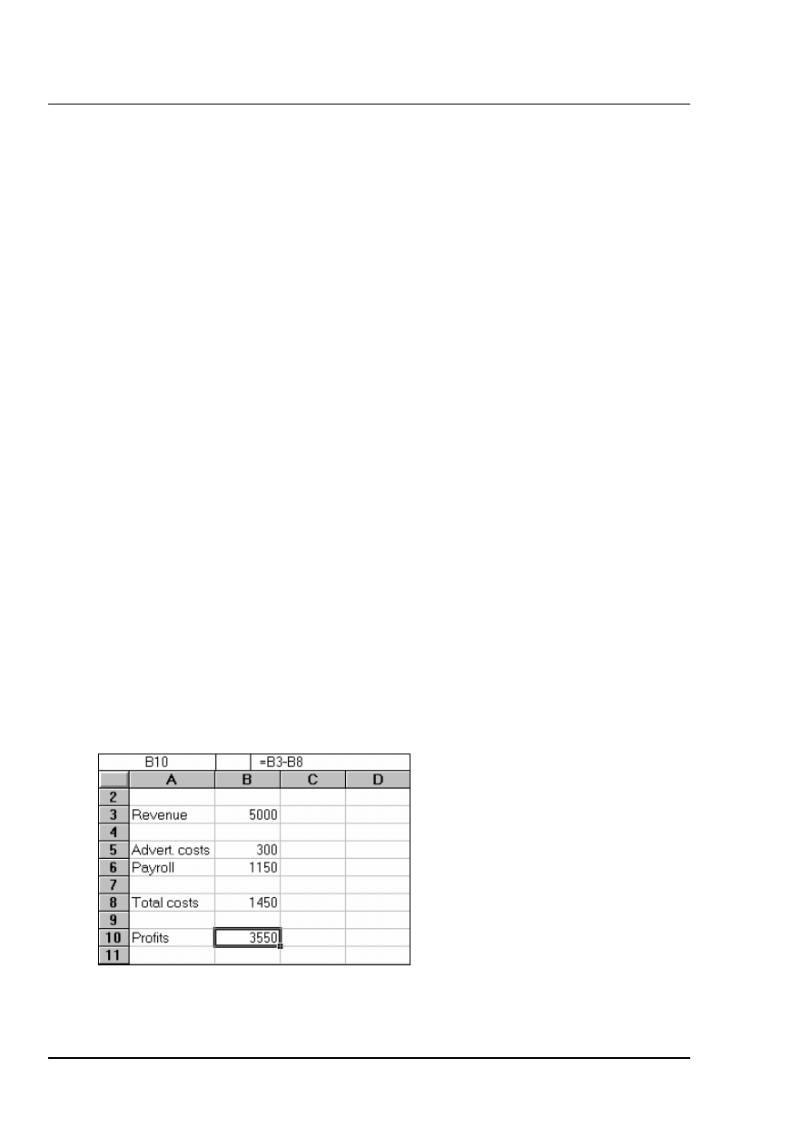
example, a time period is entered in cell A54 and in B54 the VLOOKUP formula is
contained;
Excel 2002 Advanced Level
Using advanced Worksheet functions
Page
30
Cell B54 holds this formula;
=VLOOKUP(A54,C43:H48,5)
The cell A54 is the lookup_value (time period), the table_array is as before, and for this
example rates are looked up for a loan of £40000, hence the column_index_number 5. By
changing the value of cell A54, the appropriate rate for that time period is returned.
Where the specific lookup_value is not found, VLOOKUP works in the same way as
HLOOKUP. In other words, the nearest value in the array that is less than the
lookup_value will be returned. So, a £40000 loan over 17 years would return an interest
rate of 16.00%.
NESTED LOOKUPS
One of the limitations of the horizontal and vertical LOOKUP functions is that for every
lookup_value changed, the column or row index number stays constant. Using our
example, the HLOOKUP will search for any amount, but always for the same time
period. Conversely, the VLOOKUP will search for any time period, but always for the
same amount. In both cases, if you want to alter the time period and the amount the
formula must be edited to alter the column or row index number.
There is, however, a technique whereby one LOOKUP function is "nested" within
another. This looks up one value, which will then be used in a second LOOKUP formula
as a column or row index number. Using this technique allows you to, say, enter a time
period and an amount and see the correct interest rate.
Because nested LOOKUPs have more than one lookup_value, more than one array is
needed. This second array should consist of the column or row numbers to be used in the
LOOKUP formula. The example shows our main interest rates spreadsheet, with an
additional two columns of data;
© MTC Training Solutions Ltd

Excel 2002 Advanced Level
Using advanced Worksheet functions
Page
31
Column J contains all the same time periods as column C, but alongside this are numbers
2 to 6, indicating the row_index_number to be returned for the appropriate time period.
To look up this value, use a simple vector LOOKUP formula, where K50 is the required
time period, J43:J47 is the lookup_vector and K43:K47 is the result_vector;
LOOKUP(K50,J43:J47,K43:K47)
Notice there is no equals sign, because this formula is not being entered in a cell of its
own. The formula will return a value between 2 and 6 which will be used as a
row_index_number in a HLOOKUP formula. This HLOOKUP will look in the main
interest rate table for an amount typed in by you, and will respond to the
row_index_number returned from the nested LOOKUP formula. The cells J50 and K50
hold the amount and time period to be typed in by you, and the entire nested HLOOKUP,
typed in J52, is as follows;
=HLOOKUP(J50,C43:H48,LOOKUP(K50,J43:J47,K43:K47))
In the example, the time period 25 is vertically looked up in column J and the
corresponding value 5 is returned. Also, the amount 40000 is horizontally looked up in
the main table, with a row_index_number of 5. The end result is an interest rate of
18.50%. Simply by changing cells J50 and K50, the correct interest rate is always
returned for the amount and period typed in.
© MTC Training Solutions Ltd
Excel 2002 Advanced Level
Using advanced Worksheet functions
Page
32
Goal Seeking and Solving
Excel has a number of ways of altering conditions on the spreadsheet and making
formulae produce whatever result is requested. Excel can also forecast what conditions on
the spreadsheet would be needed to optimise the result of a formula. For instance, there
may be a profits figure that needs to be kept as high as possible, a costs figure that needs
to be kept to a minimum, or a budget constraint that has to equal a certain figure exactly.
Usually, these figures are formulae that depend on a great many other variables on the
spreadsheet. Therefore, you would have to do an awful lot of trial-and-error analysis to
obtain the desired result. Excel can, however, perform this analysis very quickly to obtain
optimum results. The Goal Seek command can be used to make a formula achieve a
certain value by altering just one variable. The Solver can be used for more painstaking
analysis where many variables could be adjusted to reach a desired result. The Solver can
be used to not only obtain a specific value, but to maximise or minimise the result of a
formula (e.g. maximise profits or minimise costs).
GOAL SEEK
The Goal Seek command is used to bring one formula to a specific value. It does this by
changing one of the cells that is referenced by the formula. Goal Seek asks for a cell
reference that contains a formula (the Set cell). It also asks for a value, which is the figure
you want the cell to equal. Finally, Goal Seek asks for a cell to alter in order to take the
Set cell to the required value.
In the example spreadsheet, cell B8 contains a formula that sums advertising and payroll
costs. Cell B10 contains a profits formula based on the revenue figure, minus the total
costs.
A user may want to see how a profit of 4000 can be achieved by altering payroll costs.
© MTC Training Solutions Ltd

Excel 2002 Advanced Level
Using advanced Worksheet functions
Page
33
To launch the Goal seeker:
Mouse
1.
Click on the cell whose value you wish to set. (The Set cell must
contain a formula).
2.
Choose Tools, Goal Seek from the menu, and the following dialog
box appears:
The Goal Seek command automatically suggests the active cell as the Set
cell. This can be overtyped with a new cell reference or you may click on
the appropriate cell on the spreadsheet.
3.
Now enter the desired value this formula should reach. Click inside
the TO VALUE box and type in the value you want your selected
formula to equal.
4.
Finally, click inside the BY CHANGING CELL box and either
type or click on the cell whose value can be changed to achieve the
desired result.
5.
Click the OK button and the spreadsheet will alter the cell to a
value sufficient for the formula to reach your goal. Goal Seek also
informs you that the goal was achieved;
© MTC Training Solutions Ltd

Excel 2002 Advanced Level
Using advanced Worksheet functions
Page
34
6.
You now have the choice of accepting the revised spreadsheet, or
returning to the previous values. Click OK to keep the changes, or
Cancel to restore previous values.
Goal Seek can be used repeatedly in this way to see how revenue or other
costs could be used to influence the final profits. Simply repeat the above
process and alter the changing cell reference.
The changing cell must contain a value, not a formula. For example, if you
tried to alter profits by changing total costs, this cell contains a formula
and Goal Seek will not accept it as a changing cell. Only the advertising
costs or the payroll cells can be used as changing cells.
Goal Seek will only accept one cell reference as the changing cell, but
names are acceptable. For instance, if a user had named either cells B5 or
B6 as "Advert_costs" or "Payroll" respectively, these names could be
typed in the BY CHANGING CELL box. For goal-seeking with more than
one changing cell, use the Solver.
Goal-Seeking with Charts
Goal Seek can be used in conjunction with Excel's charting facility. Usually, when [Ctrl]
is used with the mouse to select chart data, handles appear which permit dragging of the
data up or down to a particular value. This then updates the corresponding figure on the
spreadsheet. However, if the data that is dragged is the result of a formula, Goal Seek
asks which cell to change in order to make the formula equal the required value. The
following example shows a spreadsheet and embedded chart:
© MTC Training Solutions Ltd

Excel 2002 Advanced Level
Using advanced Worksheet functions
Page
35
© MTC Training Solutions Ltd
To use goal seeker with charts:
Mouse
1.
Double click to edit the chart, and then [Ctrl] click on the series
item you want to change – this could be a column or a plot point
depending on the type of graph you have.
2.
Use the black handle markers to drag up or down altering the value
of the plot point. If the plot point value you are changing is the
result of a formula, when the mouse is released, you are returned to
the spreadsheet and the Goal Seek dialog box appears.
The box informs you that you are changing the value of a cell, which is a
formula. Therefore, it asks which cell to change in order to make the
formula cell attain the value to which it was dragged.
3.
Choose the appropriate cell, and click OK. You are returned to the
chart window.

Excel 2002 Advanced Level
Using advanced Worksheet functions
Page
36
SOLVER
For more complex trial-and-error analysis the Excel Solver should be used. Unlike Goal
Seek, the Solver can alter a formula not just to produce a set value, but to maximise or
minimise the result. More than one changing cell can be specified, so as to increase the
number of possibilities, and constraints can be built in to restrict the analysis to operate
only under specific conditions.
The basis for using the Solver is usually to alter many figures to produce the optimum
result for a single formula. This could mean, for example, altering price figures to
maximise profits. It could mean adjusting expenditure to minimise costs, etc. Whatever
the case, the variable figures to be adjusted must have an influence, either directly or
indirectly, on the overall result, that is to say the changing cells must affect the formula to
be optimised. Up to 200 changing cells can be included in the solving process, and up to
100 constraints can be built in to limit the Solver's results.
Solver Parameters
The Solver needs quite a lot of information in order for it to be able to come up with a
realistic solution. These are the Solver parameters
To set up the Solver:
Mouse
1.
Choose Tools, Solver from the menu. A dialog box appears as
follows:
© MTC Training Solutions Ltd

Excel 2002 Advanced Level
Using advanced Worksheet functions
Page
37
Like Goal Seek, the Set Cell is the cell containing the formula whose value
is to be optimised. Unlike Goal Seek, however, the formula can be
maximised or minimised as well as set to a specific value.
2.
Decide which cells the Solver should alter in order to produce the
Set Cell result. You can either type or click on the appropriate
cells, and [Ctrl] click if non-adjacent cell references are required.
When using a complex spreadsheet, or one that was created by someone
else, there is an option to let the Solver guess the changing cells. Usually it
will select the cells containing values that have an immediate effect on the
Set Cell, so it may be a good idea to amend this.
Constraints
Constraints prevent the Solver from coming up with unrealistic solutions.
To build constraints into your Solver parameters:
1.
In the Solver dialog, choose Add
2.
This dialog box asks you to choose a cell whose value will be kept
within certain limits. It can be any cell or cells on the spreadsheet
(simply type the reference or select the range).
3.
This cell can be subjected to an upper or lower limit, made to equal
a specific value or forced to be a whole number. Drop down the
arrow in the centre of the Constraint box to see the list of choices:-
To set an upper limit, click on the <= symbol; for a lower limit, >=;
the = sign for a specific value and the int option for an integer
(whole number).
4.
Once the OK button is chosen, the Solver Parameter dialog box re
displays and the constraint appears in the window at the bottom.
This constraint can be amended using the Change button, or
removed using the Delete button.
© MTC Training Solutions Ltd

Excel 2002 Advanced Level
Using advanced Worksheet functions
Page
38
When maximising or minimising a formula value, it is important to include constraints
which set upper or lower limits on the changing values. For instance, when maximising
profits by changing sales figures, the Solver could conceivably increase sales to infinity.
If the sales figures are not limited by an upper constraint, the Solver will return an error
message stating that the cell values do not converge. Similarly, minimising total costs
could be achieved by making one of the contributing costs infinitely less than zero. A
constraint should be included, therefore, to set a minimum level on these values.
The example here shows the number of cases for five London hospitals, split into three
types: Elective, Emergency and Day cases. Below this are the respective costs of each
type of case for each hospital, and finally the total costs (number multiplied by price) for
each type in each hospital. All these figures are totalled in column H, to arrive at a final
total costs figure in cell H17.
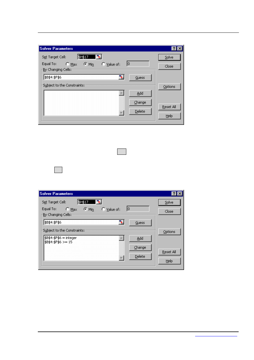
Call up the Tools, Solver command from the menu. The Set Cell in this case will be H17,
the total costs cell. It can be assumed that the costs of cases cannot be changed, only the
number in each hospital, therefore the changing cells will be B4:F6:
© MTC Training Solutions Ltd
Excel 2002 Advanced Level
Using advanced Worksheet functions
Page
39
The problem is that, if Solve is chosen now, the number of cases could reduce to
infinitely below zero and produce an error message. Fortunately, constraints can be built
in to force each hospital to have a minimum number of cases, and for there to be a total
number of cases overall. Choose the Add option to add a constraint, highlight the cells
B4:F6, drop down the arrow and click on >= to set a minimum limit. Here, type whatever
the minimum number of cases should be. To avoid the error message, simply type 1 and
choose OK. Also, as hospital cases cannot be fractions, add another constraint to force
these cells to be integers. Finally, a constraint could be added to set a total number of
cases (cell H7). The Solver parameters should now appear as follows:
When Solve is chosen, the Solver carries out its analysis and finds a solution. This may be
unsatisfactory, as it has calculated that the best way to minimise costs is to put the
majority of cases in St George's as day patients. Further constraints could now be added
to force the Solver to place minimum numbers of cases in the other hospitals, or set a
maximum limit on St Georges' day cases.
© MTC Training Solutions Ltd

Excel 2002 Advanced Level
Using advanced Worksheet functions
Page
40
Solver and Scenario Manager
The Solver uses sophisticated numeric analysis and iterative methods to perform trial-
and-error calculations very quickly. The original values of the spreadsheet, therefore,
have a profound effect on the result of a Solver solution. It may be the case that there is
no concrete solution to a spreadsheet problem, and the Solver may produce a "best guess"
within the specified constraints. Changing the original values and running the Solver
again may produce a different result, and it may therefore by helpful to save the different
"scenarios" that are produced. It may also be necessary to save scenarios where
constraints have either been added, removed or amended. Using Excel's Scenario
Manager can facilitate this, by allowing you to save each new Solver solution and
compare it to previous ones. For most complex spreadsheet problems, the Solver and
Scenario Manager are used together.
Saving Solver Solutions
When the Solver finds a solution that seems feasible, you may want to save it.
Save a solution as a Scenario:
Mouse
1.
Once Solver has found a solution, choose Save Scenario from the
dialog box. The scenario can be named and either the new values
kept or the original values restored.
To view a saved Scenario:
Mouse
1.
To see those results again, choose Tools, Scenarios from the menu,
and all named scenarios will be listed;
© MTC Training Solutions Ltd

Excel 2002 Advanced Level
Using advanced Worksheet functions
Page
41
© MTC Training Solutions Ltd
2.
Click on the appropriate name and choose Show to display the
results. Typically, a scenario only holds the results of the changing
cells set in any Solver Parameters. Choosing Edit from the
Scenario Manager allows these values to be changed, or the
Scenario renamed.

Excel 2002 Advanced Level
Using advanced Worksheet functions
Page
42
Reports
Once a Solver solution is obtained, a report can be generated to summarise the changes
that have been made and how accurately the constraints have been satisfied. When
changing cells have integer constraints, the only meaningful type of report is an Answer
Report, which gives details of the target cell's original value and new value, the changes
to the adjustable cells as well as all constraints.
To create a solver report:
Mouse
1.
Click Answer Report from the Solver Solution dialog box.
Excel generates the report in a new window behind the current
worksheet.
2.
To see the report, choose Window, Answer Report 1 from the
menu:
© MTC Training Solutions Ltd

Excel 2002 Advanced Level
Using advanced Worksheet functions
Page
43
© MTC Training Solutions Ltd
☺
Useful Information
Typical Solver Models
It is usual to employ the Solver with relatively large spreadsheets, or where lots of
variable data combine to produce a single formula result, such as a net profit figure or a
total cost figure. In the EXCEL\EXAMPLES\SOLVER sub directory, there are a number
of example worksheets which are suitable for use with the Solver.

Excel 2002 Advanced Level
Using advanced Worksheet functions
Page
44
© MTC Training Solutions Ltd
.
Notes

Excel 2002 Advanced Level
Using advanced Worksheet functions
Page
45
© MTC Training Solutions Ltd

Excel 2002 Advanced Level
Views, Scenarios & Reports
Page
46
© MTC Training Solutions Ltd
Section 2
Views, Scenarios & Reports
By the end of this section you will be able to:
Create Views
Switch between Views
Create Scenarios
Switch between Scenarios
Print Views and Scenarios in a report

Excel 2002 Advanced Level
Views, Scenarios & Reports
Page
47
Views & Scenarios
Excel's Custom Views are used to save and recall different display settings and print
options. The Scenario Manager allows you to store changes to spreadsheet data and
perform "what if" analysis.
Custom Views
Custom views allow you to save different display and print settings, and impose them
quickly and easily on the worksheet at any time. The settings which can be saved include
print settings, row heights and column widths, display settings, selected cells, window
size and positions, settings for panes and frozen titles. This can be advantageous when
dealing with large worksheets where switching from one area to another might otherwise
be awkward. It also allows a number of different print settings - including print area - to
be saved as part of the same worksheet file.
Typical Custom View Model
In the example above, Sales, Costs and Profits data can be seen at the top of the screen,
with an embedded line chart underneath. There is also an embedded pie chart, which, at
the moment, can only be seen by scrolling down the spreadsheet. It would be useful to be
able to "swap" between the line chart and the pie chart while still able to see the
spreadsheet figures. It may also be helpful to define different page settings, depending on
© MTC Training Solutions Ltd
Excel 2002 Advanced Level
Views, Scenarios & Reports
Page
48
whether the line chart or pie chart are being printed. By defining different spreadsheet
"views", it is possible to toggle between the different charts and keep the data on the
screen at all times. It is also possible to print a different header when a different type of
chart is displayed.
Defining a View
Before defining a view, you should ensure that the display options, zoom percentage,
print settings etc. are as you wish to record them.
To create a view:
Mouse
1.
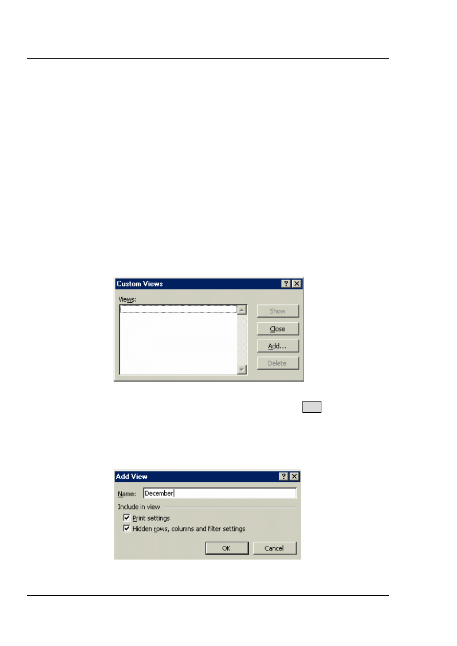
Click View from the menu bar and choose Custom Views. The
following dialog box will appear:
2.
From the Custom Views dialog box, choose Add.
3.
Choose whether or not to include print settings or hidden rows and
columns as part of the View by checking the required options.
© MTC Training Solutions Ltd

Excel 2002 Advanced Level
Views, Scenarios & Reports
Page
49
© MTC Training Solutions Ltd
4.
Enter the name under which this view is to be saved and click on
OK.
Once a view has been defined, the display and print settings of the worksheet can be
changed (for example in our typical model you may want a view to display the pie chart
next to the data with an appropriate header when printing). You can then set up a View
that would save those settings.
Showing a View
Having defined as many views as are needed for the current worksheet, you can switch
between them.
To show a view:
Mouse
1.
Choose Window, View, then highlight the name of the desired
view.
2.
Click on the Show button. If Print or Print Preview commands are
executed, the correct settings (including the header) will be apply
to each view.
To delete a view:
Mouse
1.
Choose Window, View, then highlight the name of the desired
view.
2.
Click the Delete button.
Scenario Manager
The purpose of the Scenario Manager is to allow you to save a number of alternative
inputs for specific cells which affect the results in a worksheet. For example, you may
want to see the results of changes in costs figures, and their impact on profits. A variety
of different costs figures could be saved as different "scenarios", and each one loaded in
turn to produce comparisons.
Excel 2002 Advanced Level
Views, Scenarios & Reports
Page
50
Load the Scenario Manager
Once you have constructed your worksheet with the appropriate data and formulae, you
are ready to set up scenarios.
To set up scenarios:
Mouse
1.
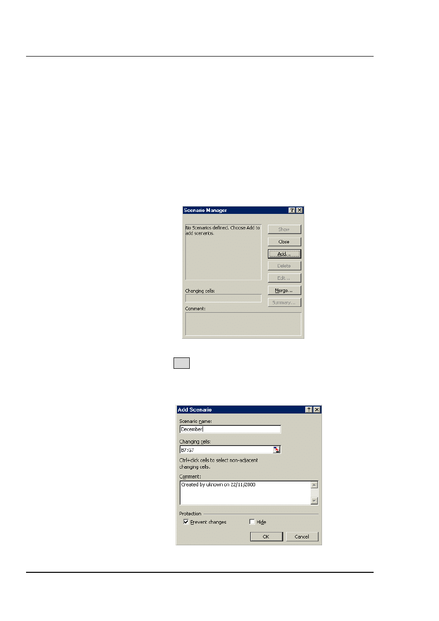
Choose Tools from the menu bar and click Scenarios. The
Scenario Manager dialog box will appear:
2.
Click the Add button to name your scenario and define the
Changing cells
(the cells containing the values you want to
vary for each scenario). The following dialog will appear:
© MTC Training Solutions Ltd

Excel 2002 Advanced Level
Views, Scenarios & Reports
Page
51
3.
Type a name in the box marked
Scenario name
.
4.
Click the button to the right of the
Changing Cells
box to
collapse the dialog allowing you to view the worksheet and select
the cells containing the variables. Non consecutive cells may be
selected using [Ctrl] and click. Click the button to expand the Add
Scenario dialog once more.
5.
Click OK to add the Scenario. The following dialog box will
appear:
6.
Type the value for the first changing cell that you want to save
under the current scenario name. Press [TAB] to move to the next
changing cell and type a value for that changing cell. Repeat the
process until all changing cell values have been set for the current
scenario.
7.
Click the OK button to return to the Scenario Manager dialog
8.
Click OK again to exit the Scenario Manager.
Or
Click the Add button to define another scenario.
9.
When all scenarios have been added, click OK to return to the
Scenario Manager dialog and OK to exit the Scenario Manager.
Showing a Scenario
When several scenarios have been created, each one in turn can be shown. The values
associated with that scenario will appear in the designated Changing Cells, and all the
dependant formulae on the worksheet will update. Any charts dependant on the changing
© MTC Training Solutions Ltd

Excel 2002 Advanced Level
Views, Scenarios & Reports
Page
52
values will also update. The Scenario Manager dialog box will remain on screen,
allowing you to click on an alternative scenario name and show it instead.
To show scenarios:
Mouse
1.
Choose Tools from the menu bar and click Scenarios. The
Scenario Manager dialog box will appear listing saved scenarios:
2.
Double-click the scenario name whose values you want on the
worksheet. The values will appear in the changing cells.
3.
The dialog box remains on-screen allowing you to double-click
other scenario names and see how the changing values affect the
data. Click OK to exit the Scenario Manager dialog.
Editing a Scenario
There are two main ways in which you might wish to change an existing scenario. You
might want to amend the values of the changing cells, or add or delete changing cells.
The approach is slightly different for each of these tasks.
© MTC Training Solutions Ltd

Excel 2002 Advanced Level
Views, Scenarios & Reports
Page
53
© MTC Training Solutions Ltd
To change values in a scenario
Mouse
1.
Choose Tools, Scenarios to open the Scenario Manager dialog box.
2.
Select the name of the scenario to be edited.
3.
Click on the Edit button and click OK from the Edit Scenario
dialog.
4.
Change the values as required, and click on the OK button. This
procedure can be repeated if necessary to edit other scenarios.
To add changing cells:
Mouse
1.
Choose Tools, Scenarios to open the Scenario Manager dialog box.
2.
Select the name of the scenario to be edited.
3.
Click on the Edit button and click the button to the right of the
Changing cells
box to collapse the Edit Scenario dialog.
4.
Hold down the [CTRL] key as you click and drag across the cells
that you want to add. Click the button to expand the dialog.
5.
Click OK to confirm the addition.
6.
Enter the value for the newly added changing cell in the Changing
cells dialog and click OK to confirm.
7.
Click Close to exit the Scenario Manager.
To remove changing cells:
Mouse
1.
Choose Tools, Scenarios to open the Scenario Manager dialog box.
2.
Select the name of the scenario to be edited.
3.
Click on the Edit button.

Excel 2002 Advanced Level
Views, Scenarios & Reports
Page
54
© MTC Training Solutions Ltd
4.
Drag across the cell references of the cells you want to remove
from the
Changing cells
box and press [DELETE].
5.
Click OK to confirm the deletion and OK again to close the
Changing cells dialog.
6.
Click Close to exit the Scenario Manager.
Deleting a Scenario
To delete a scenario:
Mouse
1.
Choose Tools, Scenarios to open the Scenario Manager dialog box.
2.
Select the name of the scenario to be deleted.
3.
Click Delete button.
You can’t undo the deletion of a scenario.
Print Reports
When you have Views and/or Scenarios defined in one worksheet, there are occasions
where you want to print all the views, perhaps with each of the scenarios. Rather than
accessing each view and scenario in turn and manually sending them to print, Excel
allows you to send them all together by creating a report.
The Report Manager
The tool you use to build reports is the Report Manager. This allows you to specify the
sections you want in your report. Sections can be a defined View which you can also
combine with a Scenario if necessary. Each section will print on a separate page.
To access the Report Manager:
Mouse
1.
Choose View from the menu bar and click Report Manager. The
following dialog box will appear:-
Excel 2002 Advanced Level
Views, Scenarios & Reports
Page
55
Create a Report
Once the Report Manager dialog is displayed, you can create new reports using the
defined Views and Scenarios, edit existing reports or delete them.
To add a report:
Mouse
1.
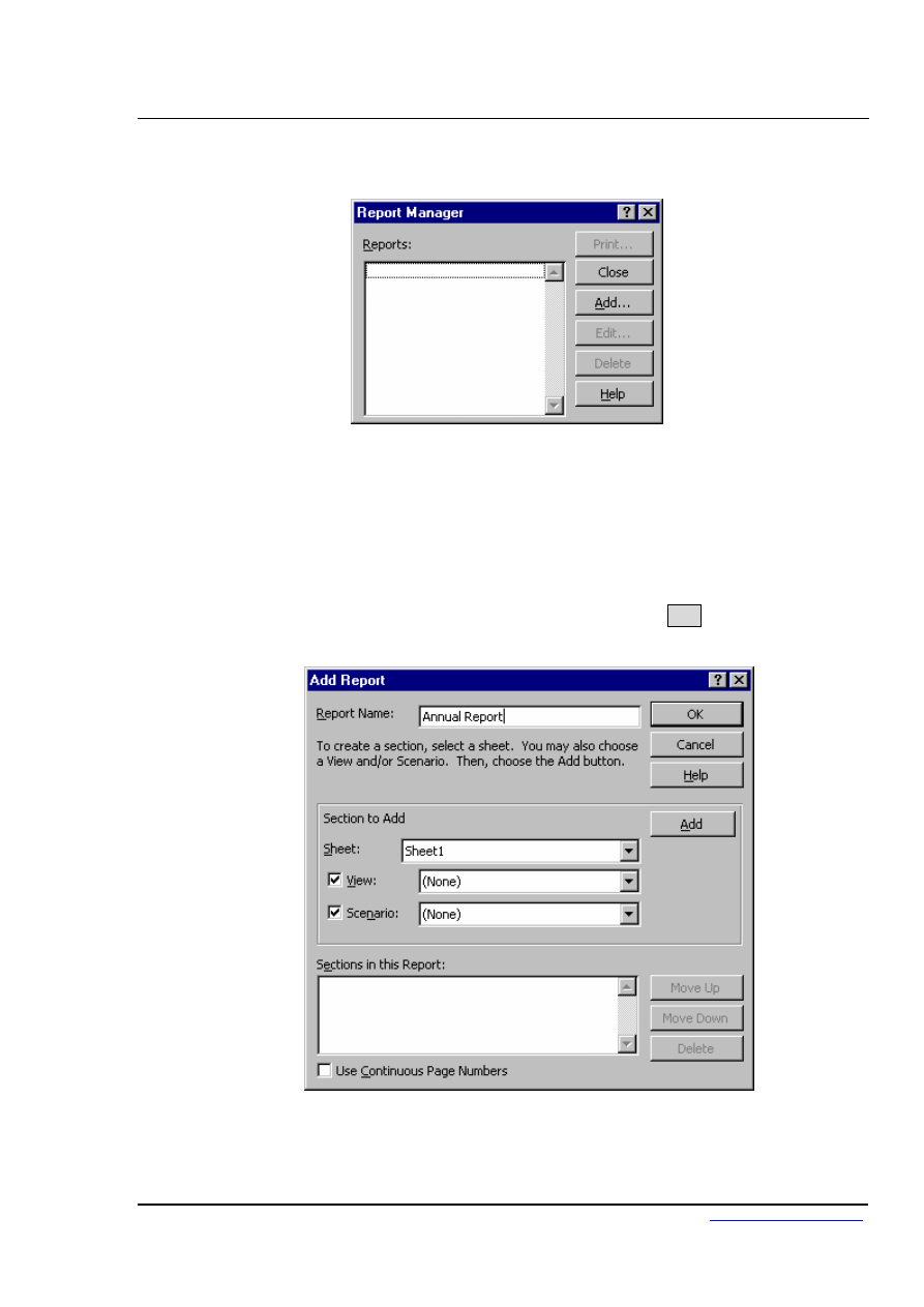
From the Report Manager dialog, click the Add button. The
following dialog box will be displayed:-
2.
Type a name for your report in the
Report Name
text box.
© MTC Training Solutions Ltd

Excel 2002 Advanced Level
Views, Scenarios & Reports
Page
56
3.
Select the sheet containing the Views and Scenarios you have
defined by clicking the drop-down list arrow to the right of the box
labelled
Sheet
.
4.
Build the sections by choosing a View from the drop-down list
labelled
View
, and a Scenario from the drop-down list labelled
Scenario
. Click the Add button to add the section to the report.
5.
Repeat steps 3 and 4 until you have built all the sections you want
to print. They will appear listed in the
Sections in this
Report
box at the bottom of the dialog.
6.
If you want to reorganise the sections, click the section you want to
move and use the Move Up and Move down buttons to position it
in the correct place. You can also delete a selected section with the
Delete button.
7.
If you want consecutive page numbering throughout your report,
check the
Use
Continuous Page Numbers
box.
8.
Click the OK button to save the Report and return to the previous
dialog.
You don’t have to include both a View and a Scenario per section. If your
report only comprises Views, uncheck the Scenario box and conversely, if
your report only comprises Scenarios, uncheck the Views box.
© MTC Training Solutions Ltd

Excel 2002 Advanced Level
Views, Scenarios & Reports
Page
57
Print a Report
Once your report has been set up, you can send it to print. There is no facility to preview
what the hard copy of your report will look like, however, when you issue the print
command, Excel will actually run through each view and scenario on-screen, before
sending it to the printer.
To print a report:
Mouse
1.
Choose View from the menu bar and then Report Manager.
2.
Click the report that you want to print and then click the
button.
3.
Type the number of copies of the report you want to print and click
OK.
Edit a Report
You may need to change a report subsequent to setting it up.
To edit a report:
Mouse
1.
Choose View from the menu bar and then Report Manager.
2.
Click the report that you want to print and then click the
Edit
button.
3.
Make changes to the report by adding new sections, deleting
sections or reorganising them (see the section entitled Create a
report earlier in this section for details).
4.
Click OK to save the changes.
© MTC Training Solutions Ltd
Excel 2002 Advanced Level
Views, Scenarios & Reports
Page
58
Delete a Report
Reports you have set up in any one work session are saved when you save the file. If you
want to delete them, you can do so using the Report Manager dialog.
To delete a report:
Mouse
1.
Choose View from the menu bar and click Report Manager.
2.
Select the report that you want to delete and click the
Delete
button.
3.
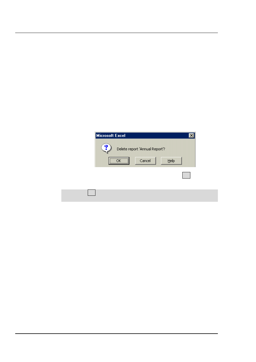
Excel will ask you to confirm the deletion. Click OK to delete the
report or cancel to abandon the deletion.
If you click OK when Excel asks you if you want to delete a report, you
can’t undo the deletion.
© MTC Training Solutions Ltd

Excel 2002 Advanced Level
Views, Scenarios & Reports
Page
59
© MTC Training Solutions Ltd
☺
Useful Information
Rather than recording macros to set print areas throughout a workbook and print them
out, define them as Views first. Your macro only then needs to record you switching to
each View in turn and printing it.

Excel 2002 Advanced Level
Views, Scenarios & Reports
Page
60
© MTC Training Solutions Ltd
.
Notes

Excel 2002 Advanced Level
Views, Scenarios & Reports
Page
61
© MTC Training Solutions Ltd

Excel 2002 Advanced Level
Using Excel to Manage Lists
Page
62
© MTC Training Solutions Ltd
Section 3
Using Excel to Manage Lists
Objectives
By the end of this section you will be able to:
Set up an Excel list
Sort the list
Create list subtotals
Add, edit and delete list items using the data
form
Use AutoFilter to find specific list data
Use the Advanced filtering tools
Analyse list data with data and pivot tables

Excel 2002 Advanced Level
Using Excel to Manage Lists
Page
63
© MTC Training Solutions Ltd
Excel Lists
Although Excel's primary function is as a Spreadsheet, it can also be used for a number of
list operations. It is possible to store, and manipulate information (customer records, staff
records, or stock inventories for example) on an Excel worksheet, organise it in different
ways, and "query" the list to extract information which meets specific, user-defined
criteria. The list is effectively treated as a database.
In order to use Excel's database capacity, information must be laid out in rows and
columns subject to certain constraints. There are some database terms with which the
user should become familiar:
List Terminology
Row and column content
The information being stored must be divided up into categories. For example,
information on staff might include Firstname, Lastname, and Department. In an Excel
List, each category must be entered in a separate column. Do not mix text and numbers
in a column – the data must belong to the same category of information and therefore
should be the same data type. Do not use spaces in front of column entries, use alignment
buttons instead if you need to move data away from the column edges.
Column labels
This is the title at the top of each column, describing the category of information which it
contains. Each label name must be unique and must be made up of text rather than
numbers or calculations. The column names must appear directly above the list
information - they may not be separated from the rest of the list by a blank row. Format
your column labels to distinguish them from the list data.
List size and location
The List is the whole collection of information, all Fields, Fieldnames and Records and
should be laid out as a regular block of data.
• A list can be up to 256 columns wide by 65536 rows (an entire worksheet).
• Do not place more than one list on a worksheet. If you want more than one list in a
workbook, place each list on a separate sheet.

Excel 2002 Advanced Level
Using Excel to Manage Lists
Page
64
© MTC Training Solutions Ltd
• Leave at least one blank row and one blank column between the list and other data on
the worksheet.
• Place additional data diagonally below and to the right of your list. This ensures that
data will not be affected when you filter the list.
Miscellaneous
• Excel does not distinguish between upper and lower case characters in a list, unless
you use the Case-sensitive sort option.
• When you use formulae in lists, Excel uses the results of the formulae.

Excel 2002 Advanced Level
Using Excel to Manage Lists
Page
65
Sorting Data
Although not confined to database information, the sorting facility in Excel is particularly
appropriate for changing the order in which records are listed. Remember to save the file
containing the database information prior to sorting.
If you will need to restore the original record order, it is a good idea to include a column
of record numbers before sorting the database. This can be achieved simply by adding a
column with a suitable heading, and using the fill handle or the data series command to
enter consecutive numbers adjacent to each record.
To perform a single-level sort:
Mouse
1.
Select a cell in the list within the column by which you want to
sort.
2.
Click the Sort Ascending or Sort Descending button from the
toolbar.
Excel automatically selects the entire list for sorting. It compares the top
rows of your list for formatting differences. If there is a difference in the
formatting of the top row, Excel identifies that row as column labels and
excludes it from the sort. This ensures the column labels will not be sorted
with the rest of the data.
To perform a multi-level sort:
Mouse
1.
Select the data to be sorted. This will include all fields and all
records, including the field names.
Ensure that all fields are selected, otherwise part of each record will be
sorted, while part remains stationary. This could result in situations
where a client name is listed beside the wrong address.
2.
Choose Data, from the menu bar, then Sort... The following dialog
box will appear in which from which you may specify the Sort
fields and the Sort order.
ta, from the menu bar, then Sort... The following dialog
box will appear in which from which you may specify the Sort
fields and the Sort order.
© MTC Training Solutions Ltd

Excel 2002 Advanced Level
Using Excel to Manage Lists
Page
66
3.
From the Sort By drop-down list, select the field you want to use
as the main sort order. Select the Ascending or Descending radio
buttons depending on which order you wish the data sorted in.
4.
Specify any sub-sorts using the Then By drop-down lists to pick
the subsequent fields to sort by when duplicates occur in the main
sort field.
5.
Click OK.
Although there appears to be a maximum of three sort keys available, the user can in fact
manipulate the database with a series of sorts to achieve the same results as if there were
several sort keys. Excel will observe any sort keys specified, but where there are
duplicates and no subsequent sort key to differentiate between them, Excel will maintain
the order from previous sorts. In this way, if the user wishes to sort using more than three
sort keys, sort on the least important keys first, then on the more important ones in a
second operation.
Custom Sorting Options
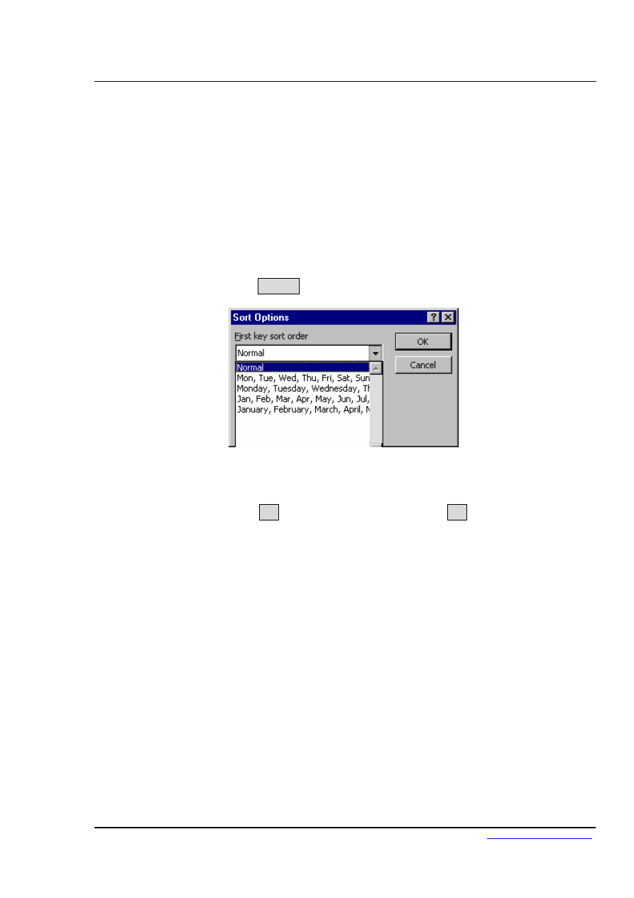
The ascending and descending sort orders rearrange your list by alphabetical, numerical,
reverse alphabetical or reverse numerical order. For some types of data, such as months,
this may not be the order that you need to use. You can use one of the custom sort orders
provided with the Excel program to rearrange your data in chronological order by day of
the week or by month.
© MTC Training Solutions Ltd
Excel 2002 Advanced Level
Using Excel to Manage Lists
Page
67
To sort by a custom sort order:
Mouse
1.
Place the active cell within the list.
2.
Choose Data from the menu bar, then Sort.
3.
From the Sort By drop-down list, select the column by which you
want to sort.
4.
Click on Options.
5.
From the First Key Sort Order drop-down list, select a custom
sort order.
6.
Click on OK to return to the Sort dialog and OK again to perform
the sort.
Creating a custom sort order
When sorting by ascending, descending or chronological order is not suitable for the data
in a list, you can create a custom sort order. Custom sort orders enable you to give Excel
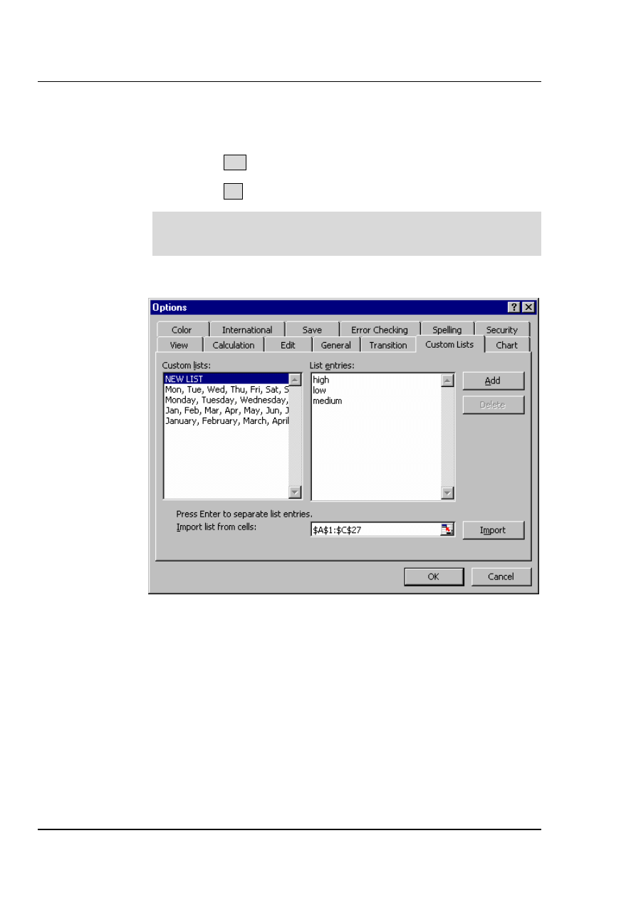
the exact order to rearrange data. Custom sort orders are helpful for data such as Low,
Medium, High, where neither alphabetical nor an existing custom sort order will provide
the desired results.
To create a custom sort order:
Mouse
1.
Choose Tools from the menu bar, then Options.
2.
Activate the Custom Lists tab.
3.
In the Custom Lists box, verify that New List is selected.
© MTC Training Solutions Ltd
Excel 2002 Advanced Level
Using Excel to Manage Lists
Page
68
4.
In the List Entries box, type each unique entry in the order you
want to sort the entries. Separate the entries by pressing [ENTER].
5.
Click Add.
6.
Click OK.
Custom sort orders are saved with the Excel ’2003 program settings and
are available for use with all worksheets. You can use a custom list with
the AutoFill feature.
© MTC Training Solutions Ltd
Excel 2002 Advanced Level
Using Excel to Manage Lists
Page
69
Adding subtotals to a list
Automatic subtotals are useful in summarising the data contained in a list. Subtotals are
created by using an Excel summary function such as SUM(), COUNT() or AVERAGE().
To use the subtotals, your data must be organised in a properly designed list and sorted
according to the column by which you want to summarise the data.
To add subtotals to a list:
Mouse
1.
Sort the list according to the column by which you want to
summarise the data.
2.
Choose Data from the menu bar, then Subtotals.
3.
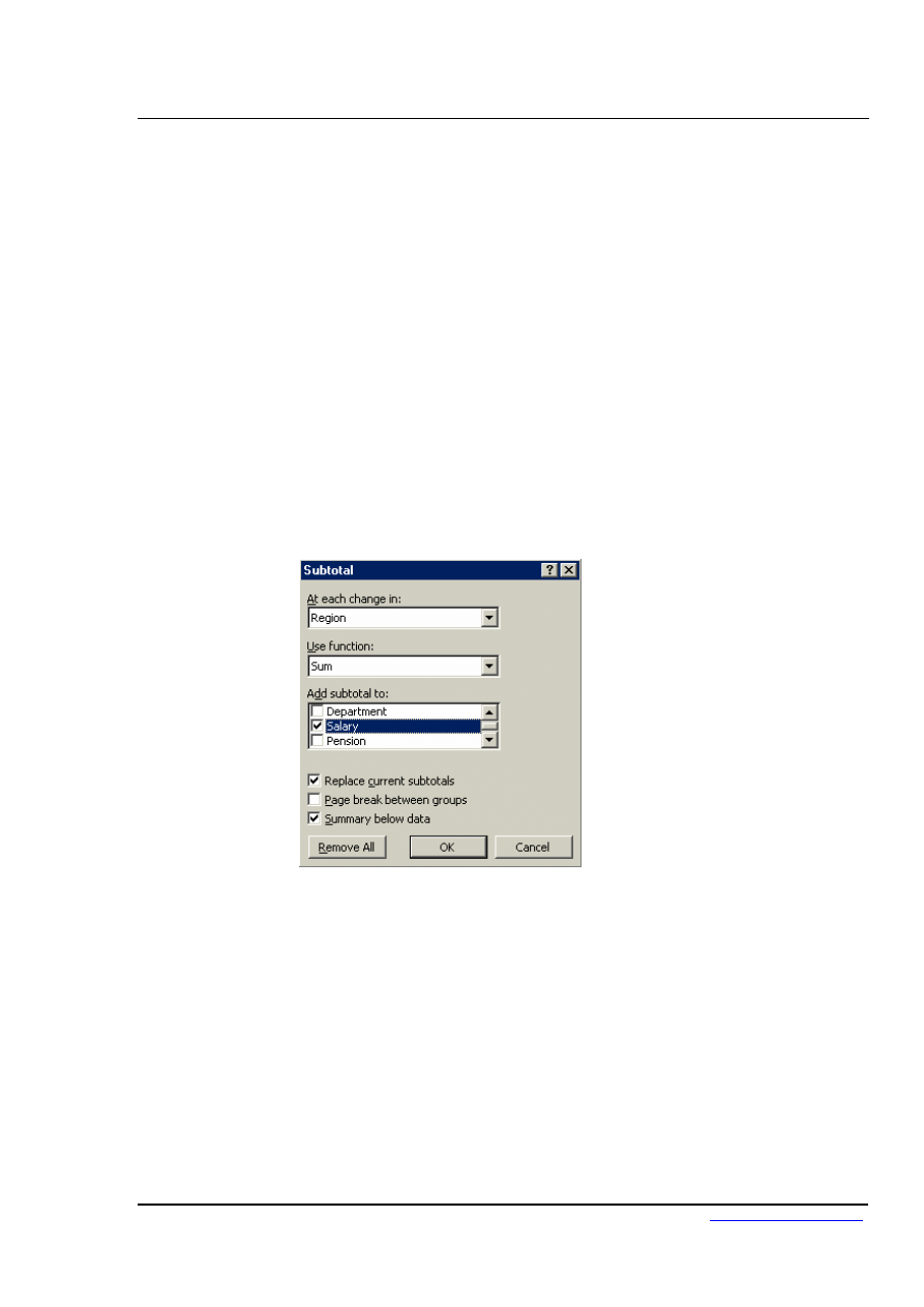
From the At Each Change In drop-down list, select the field by
which you want to summarise the data.
4.
From the Use Function drop-down list, select the summary
function you want to use to generate the subtotals.
5.
In the Add Subtotal To box, check the column to which you
want the function to be applied.
© MTC Training Solutions Ltd

Excel 2002 Advanced Level
Using Excel to Manage Lists
Page
70
© MTC Training Solutions Ltd
heck the options for replacing the current subtotals (if
any), inserting a page break for each summary group, and inserting
6.
If desired, c
the summary below each group.
7.
Click OK.
When you use the Data, Subtotals command, it adds its own Grand Total,
so you should not use the SUM() function in your list. If you use the Data,
Subtotals command, the SUM() function will be inaccurate since it
includes the subtotals in the calculation.
To
mo
thin the subtotalled list.
2.
Choose Data from the menu bar, then Subtotals.
re
ve subtotals from a list:
Mouse
1.
Select a single cell somewhere wi
3.
Click Remove All and then OK.
Examining subtotals
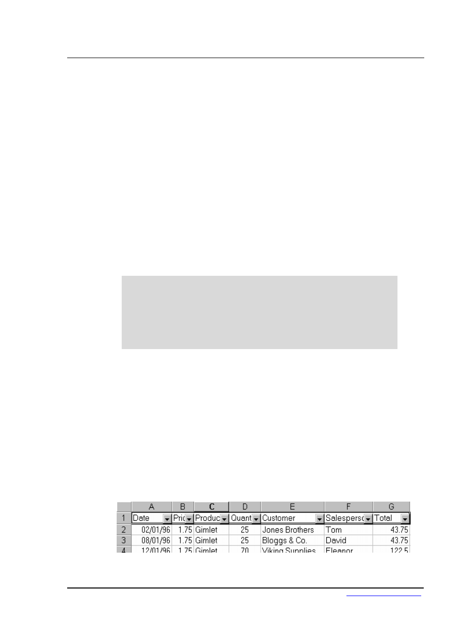
When you insert automatic subtotals, Excel creates an outline of your data. The outline
enables you
e outline buttons
below the Nam
the list data,
not the subtotal rows.
to show or hide certain sections of data by clicking on th
e box on the formula bar. Grand total values are derived from
Outline
buttons
Excel 2002 Advanced Level
Using Excel to Manage Lists
Page
71
Filtering a List
When you filter a list, you display only the sets of data that meet a certain set of search
conditions called criteria. The AutoFilter feature enables you to specify those search
conditions from the list.
When you use the Data, Filter, AutoFilter command, drop-down list arrows are displayed
next to each of the column labels in the list. When you open a drop-down list, a list of all
the unique entries for that column is displayed. By selecting one of the entries from the
drop-down list, called a filter criterion you instruct Excel what to search for. Then Excel
filters the list so that only the sets of data that contain the entry you selected will be
displayed. When Filter mode is active, arrows for the columns with filter criterion
selected appear in blue on the worksheet, row numbers appear in blue, and the status bar
displays either the number of rows that meet the criteria, or the text “Filter mode”. The
sets of data that do not meet the criteria remain in the list but they are hidden.
If you select a single cell in the list before choosing Data, Filter,
AutoFilter, drop-down list arrows are applied to all of the column labels
in your list. If you select multiple column labels before choosing Data,
Filter, AutoFilter, drop-down list arrows are displayed only for the
selected columns, thus restricting which columns you can apply filters to.
In either case, the entire list is filtered. Also, you can filter only one list at
a time on a worksheet.
To filter a list using AutoFilter:
Mouse
1.
Place the active cell anywhere within your list.
2.
Choose Data from the menu bar, Filter, AutoFilter. Your list
column labels will appear with drop-down list arrows to the right.
3.
Click the drop-down arrow for the column that you want to filter
by to display the unique values from that column. Select the value
you are filtering for.
© MTC Training Solutions Ltd

Excel 2002 Advanced Level
Using Excel to Manage Lists
Page
72
© MTC Training Solutions Ltd
4.
Repeat step 3 until you have set filter criteria for all columns that
you wish to filter by.
5.
The list will show only those rows that match your criteria.
Whilst a filter is active, if you print the worksheet, only visible rows will be
output, so you can print out multiple views of your data from an individual
list.
Removing a single column filter:
Mouse
1.
You can see which columns have filter criteria active because the
drop-down list arrows are blue. Click the drop-down list arrow for
the column whose criteria you wish to remove.
2.
Select All at the top of the list.
Removing all column filters:
Mouse
1.
Choose Data from the menu bar, then Filter, Show All.
Custom criteria
When you specify a filter criterion for a column from unique entries listed in the
AutoFilter drop-down list, you can only select one filter criterion at a time. The Custom
filter criterion enables you to filter a list to display sets of data that contain either of two
unique entries in a column. This creates an OR condition. To meet the filter criteria, a
set of data must meet either the first filter criterion or the second filter criterion.
You can also use the Custom criterion choice to find values that fall within a range.
When you specify custom criteria, select a comparison operator from the drop-down list
and then either type in a value or select it from the criteria drop-down list.
When you use custom criteria, you need to understand the comparison operators that
Excel offers you. The table below outlines these:
Excel 2002 Advanced Level
Using Excel to Manage Lists
Page
73
© MTC Training Solutions Ltd
Operator Meaning
= Equal
to
> Greater
than
< Less
than
>=
Greater than or
equal to
<=
Less than or equal
to
<>
Not equal to
To specify “either/or” custom criteria:
Mouse
1.
Click on the AutoFilter drop-down for the desired column.
2.
Select Custom.
3.
In the Custom AutoFilter dialog box from the first criteria drop-
down list select one of the filter criteria. (The default operator is
=).
4.
Click on Or.
5.
From the second operator drop-down list, select a comparison
operator.
6.
From the second criteria drop-down list select the other filter
criterion.
7.
Click OK. The filtered list shows the sets of data that meet either
the first or the second specified criterion for the column.
Excel 2002 Advanced Level
Using Excel to Manage Lists
Page
74
© MTC Training Solutions Ltd
Using custom criteria to find a range of values:
Mouse
1.
Click the drop-down arrow for the column label whose range of
values you want to filter by.
This will typically be numbers or dates
2.
Click Custom. From the resulting dialog box, select the
comparison operator to control the lower limiting value, for
example > or >=.
3.
From the first criteria drop-down list, select a value or type the
value in.
4.
Click OK
Or
Choose an upper limiting value by selecting a comparison operator
from the second operator drop-down list and selecting a second
criterion from the second criteria drop-down list or typing one in.
Click OK.
Wildcards
You can use wildcards to search for text in common within the unique entries, even
though the entire entry might not match. For example, searching for all of the sets of data
that have entries in the last-name column that begin with “M” might display two Moores
(where the entire entry matches) but might also display Madding and Martinez (where the
entire entry does not match).
Wildcard Finds
Example
*
asterisk
Any set of characters
that are in the same
position as the asterisk
*.xls finds Filter.xls and
sortdata.xls
? question mark
Any
single
character
that is in the same
position as the ?
B?t finds Bat, Bit, But
and Bet
~ tilde
A question mark or an
asterisk
Who~? Finds the text
“Who?”

Excel 2002 Advanced Level
Using Excel to Manage Lists
Page
75
© MTC Training Solutions Ltd
To filter a list using wildcards:
Mouse
1.
With AutoFilter active, select the drop-down list arrow to the right
of the column you want to use to filter the data.
Wildcards only work when filtering columns containing text
2.
Choose Custom.
3.
Ensure that the operator is set to =.
4.
Type the pattern of letters you are filtering by with the asterisks
and/or question marks inserted in the appropriate positions.
5.
Click OK.
Turning off AutoFilter
When you no longer need to filter your data, you can switch the AutoFilter off in the
following way:
To switch off AutoFilter:
Mouse
1.
Choose Data from the menu bar, then Filter.
2.
The AutoFilter option on the submenu will appear ticked showing
that AutoFilter is currently active. Click AutoFilter to remove the
tick and deactivate the AutoFilter.
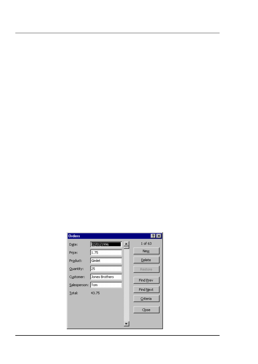
Excel 2002 Advanced Level
Using Excel to Manage Lists
Page
76
Data Form
Once the List area has been defined, you may choose to view and operate on the records
via the Excel Data Form. This is a dialog box that enables you to enter, edit or find sets
of data. Working with a data form can be a time-saving tool when maintaining data in
lists.
To activate the Data form:
1.
Click on a cell within the list.
2.
Choose Data from the menu bar, then Form..
The Data Form Screen
A dialog box will appear on screen, displaying the name of the worksheet containing the
list across the title bar. Each column name will be listed down the left hand side of the
dialog box, and the details for one record will be displayed.
Moving
There is a vertical scrollbar which can be used to move up and down through the
available records. The current record number will appear at the top right of the Data
Form, and will adjust as you move through the records.
© MTC Training Solutions Ltd
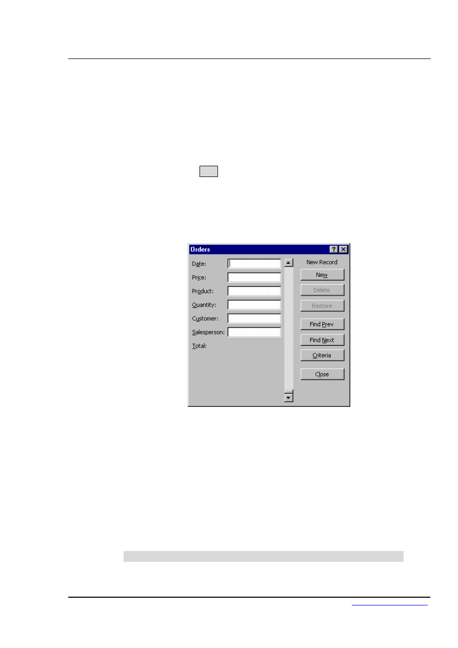
Excel 2002 Advanced Level
Using Excel to Manage Lists
Page
77
A series of buttons appears down the right hand side of the Data Form. These can be
used to perform a number of different operations on the data.
To add records using the data form:
Mouse
1.
Click on the New button to add a new record to the database.
2.
The record number display will change to New Record, and the
fields beside each fieldname will be cleared, waiting for you to
input information.
3.
Use Tab or [Shift] Tab to move from field to field.
To delete records using the data form:
Mouse
1.
Move to the record you want to delete.
2.
Click on the Delete button in order to delete the record currently on
display.
This operation cannot be reversed.
© MTC Training Solutions Ltd

Excel 2002 Advanced Level
Using Excel to Manage Lists
Page
78
© MTC Training Solutions Ltd
Edit or Restore Records
You may click in any of the text boxes and edit the information it contains. If you click
on the Restore button before moving away from the record displayed, the changes will be
undone and the original information on that record will be restored.
Search for Specific Records
It is possible to specify particular field contents and require Excel to identify those
records matching your specifications. This can be done using the Criteria button.
Entering Search Criteria
At the most basic level, either text or numeric data can be entered so that Excel will find
those records where the relevant field exactly matches what you have entered. Excel is
not case sensitive when matching criteria, so text can be entered in upper or lower case.
Excel will find those records which match the data entered in the criteria range, but will
also match any records where the initial letters match the specified data. For example,
searching for the first name Rob will find all exact matches, but will also match any
records where the first name happens to be Robert or Robin.
When using the Data Form, if you wish to confine the search results to only those records
where the first name is Rob, it would be necessary to enter the formula =Rob in the
appropriate field in the Criteria form.
Criteria Entered
Results Matched
Rob
Rob; Robert; Robin
=Rob Rob
Finding Ranges of Records
Relative or Comparison operators such as < or > can be entered with data. For example,
<25 entered in a field entitled Age would limit the view to only those persons whose age
was less than 25.
Relative Operators
Definition
= Equal
to
< Less
than
<=
Less than or Equal to
> Greater
than
>=
Greater than or Equal to
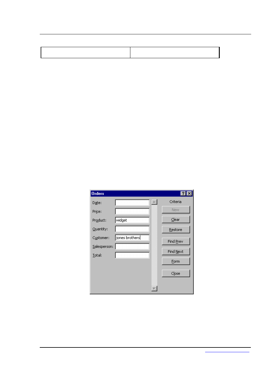
Excel 2002 Advanced Level
Using Excel to Manage Lists
Page
79
<>
Not Equal to
Comparison operators may also be used on fields containing text information. Entering
<C in a field entitled Surname would limit the view to only those persons whose name
began with either A or B.
Entering the = symbol on its own in a field would allow Excel to find those records where
that field was blank. The <> symbol on its own in a field would identify records where
that field was not blank.
Date searches may also be carried out using either exact matches or in combination with
comparison operators. To find records dated earlier than 20th January 1993, you could
enter <20/1/93.
Multiple Criteria Using the Data Form
A combination of different specifications may be entered in different fields and Excel will
find only those records which meet all specifications. For example, if you enter Widget
as the Product and Jones Brothers as the Customer, Excel will find only those orders
which fulfil both criteria.
© MTC Training Solutions Ltd

Excel 2002 Advanced Level
Using Excel to Manage Lists
Page
80
© MTC Training Solutions Ltd
To find records by setting criteria:
Mouse
1.
Click Criteria
2.
A blank form will display. Use the [TAB] key to move to the text
box for the field where you want to set the criteria and type it in.
3.
Click Find Next to jump down to the first matching record in the
list. Clicking Find Next will subsequently allow you to move
through the matching records one by one until Excel bleeps,
signalling there are no more matches. Click Find Previous to jump
to matching records in an upwards direction.
Clear Criteria
When you click the Criteria button Excel offers you a dialog where you can set criteria.
Your last criteria will have been stored and remembered and will still be visible in the
relevant text boxes.
To clear criteria:
Mouse
1.
Click the Clear button.
To return to the data form:
Mouse
1.
Click on the Form button to return you to the Data Form

Excel 2002 Advanced Level
Using Excel to Manage Lists
Page
81
Advanced Filtering
Sometimes, the filter criteria that you specify with AutoFilter will not yield the necessary
results. For example, you cannot use AutoFilter to filter a list to display the more
complex criteria of two separate AND conditions combined with an OR condition. To do
this, you must use the Advanced Filter option. This relies on you setting up and defining
a Criteria range on the worksheet where the data to be matched can be entered.
Set Criteria
The Criteria range usually consists of a copied set of the list column names, and a blank
row immediately beneath into which you can type the data to be matched. It is a good
idea to copy the column names from the top of the database into the area to be used as a
criteria range, as this reduces the chance of there being any discrepancy between the two
sets of names.
In fact, not all the column labels need to be included in the criteria range. It could be
restricted to only those labels on which you wished to search, and those labels included
could be displayed in a different order. Usually, however, the names are copied complete
from the top of the list.
To define the Criteria range:
Mouse
1.
Select the copied set of column labels and the blank row
immediately beneath them and choose Insert from the menu bar,
then Name, Define.
2.
Type the word Criteria into the name box and press [ENTER].
You do not have to name the cells with the range name Criteria, but it will
ensure that Excel automatically picks the correct group of cells as the
criteria carrying cells whenever you use the Advanced Filter.
© MTC Training Solutions Ltd

Excel 2002 Advanced Level
Using Excel to Manage Lists
Page
82
To run an advanced filter:
Mouse
1.
Enter criteria in the blank row of the criteria range under the
appropriate column label(s).
2.
Ensure that either a cell in the list is selected
3.
Choose Data from the menu bar, then Filter, Advanced Filter.
Excel will hide the records which do not match the search settings.
To remove a filter:
Mouse
1.
When finished viewing the results of the Filter operation, choose
Data, Filter, Show All.
Entering Search Criteria
At a basic level criteria entered in the Criteria range is subject to the same limitations as
were outlined in the Data Form section, but making use of a user defined Criteria range
rather than the Criteria section of the Data Form allows more complex searches to be
performed.
It is important to remember to delete old criteria before applying a new filter. Otherwise
the true results of a filter will not be shown. For example, if the first filter is applied with
Johnson entered under Surname, and a subsequent filter is carried out for those who work
in Finance, it is essential that the Name specification is cleared unless you deliberately
wish to confine the filter to those people called Johnson who happen to work in the
Finance department.
As with the Data Form, Excel will find records matching text information entered in the
Criteria range, and records where the initial letters match the specified data. When
working with a user defined criteria range, if you wish to confine filter results to only
those records where, for example, the first name is Rob, it would be necessary to enter the
formula ="=Rob" in the Criteria range under the appropriate column label.
Criteria Entered
Results Matched
Rob
Rob; Robert; Robin
© MTC Training Solutions Ltd

Excel 2002 Advanced Level
Using Excel to Manage Lists
Page
83
© MTC Training Solutions Ltd
="=Rob" Rob
Wildcards with Text Criteria
One variation on searches for text criteria consists of using text Wildcard symbols. In
fact Wildcards may be used for searches using the Data Form screen also. The two
Wildcard symbols may be familiar to users of other PC systems.
The Asterisk
The Asterisk (*) may be substituted for any group of characters. Searching for *Banking
would find both Development Banking and Merchant Banking. If no Wildcard symbols
are included in the search criteria, Excel usually assumes that there is an asterisk at the
end of the specification, so it will match the data specified and any records where the
initial data is the same.
The Question Mark
The Question Mark (?) may be substituted for any single character. The question mark
identifies the position of the wildcard character within the string of text. T?m would find
Tim or Tom. ?a would find all records where the second letter in the appropriate field
was an A. Once again, Excel will assume that there is an asterisk on the end of the search
specification unless otherwise informed. Entering T?m in a Firstname field would find
Tim, Tom and Tommy. Use the syntax ="=T?m" to confine the searches to three
characters in length.
Multiple Criteria
Hitherto, the Criteria range has been described as a copied set of field names followed by
a blank row, into which you may enter search specifications under the appropriate column
names. As with the Data Form criteria screen, you may choose to enter criteria in the
blank row under more than one field name. Entering Finance as the department and 7 as
the grade for example, would find only those persons who met both criteria.
Multiple criteria on the same row dictates that the first specification AND all other
specifications must be met in order for Excel to find the record. (See also use of the
AND() function under Calculated Criteria).
Using Multiple Rows in the Criteria Range
There may be situations where you wish to find members of either Finance or Infen. In
such an instance the Criteria range can be extended to include a second row into which
you may enter specifications:
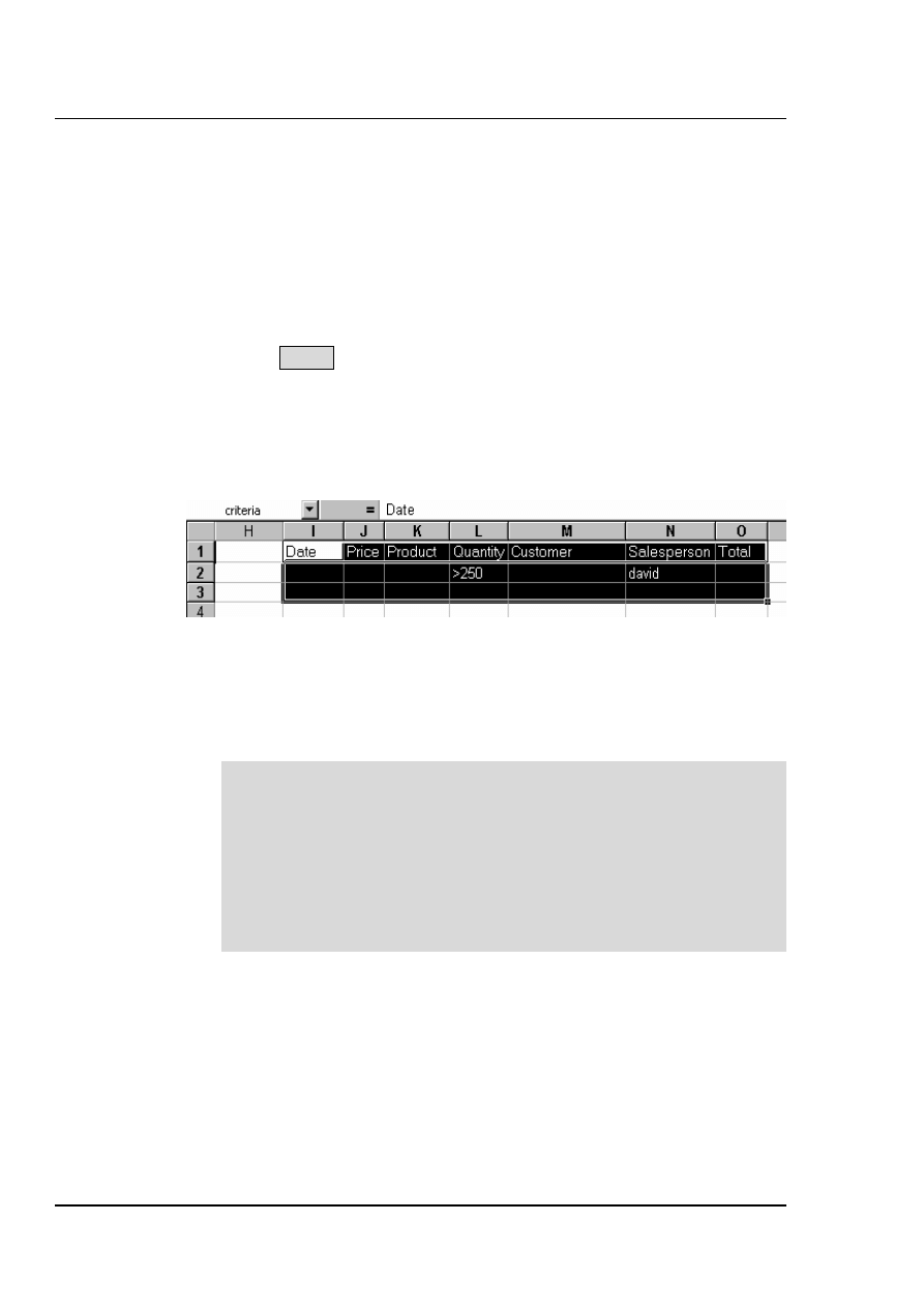
Excel 2002 Advanced Level
Using Excel to Manage Lists
Page
84
Extending the criteria range for OR criteria:
Mouse
1.
First delete the current Criteria range name. Choose Insert from
the menu bar, then Name, Define.
2.
Select Criteria from the names list inside the dialog and click
Delete.
3.
Highlight the entire region to be redefined as the Criteria range -
i.e. the copied set of Column names and the two rows (or more)
immediately below, and choose Insert from the menu bar, then
Name, Define.
4.
Type the word Criteria into the name box. and press [ENTER].
Now, entering search specifications in all rows within the range will allow Excel to
identify all those records which meet the specifications in either the first OR the second
row etc. (See also use of the OR() function under Calculated Criteria).
The Criteria range may be extended to include three or more rows of user
defined search criteria if required.
To return to using just one row of user defined information in the Criteria
range, select the area to be included and redefine the Criteria range
again. This is important because searching for data when a row in the
Criteria range has been left blank, will result in Excel finding every record
in the database. In effect, you have asked Excel to find all records where
the contents of any field can be anything at all.
Checking the Criteria range
If you are getting surprising results when you filter your data, it may be because your
criteria range contains unlabelled cells or extra rows that you thought you had removed
from the range.
It is easy to double check the currently defined Criteria range at any time by making use
of the range name which Excel applies to it. Using the [F5] function key will result in a
dialog box showing all the currently named ranges on the worksheet. Click on the name
© MTC Training Solutions Ltd
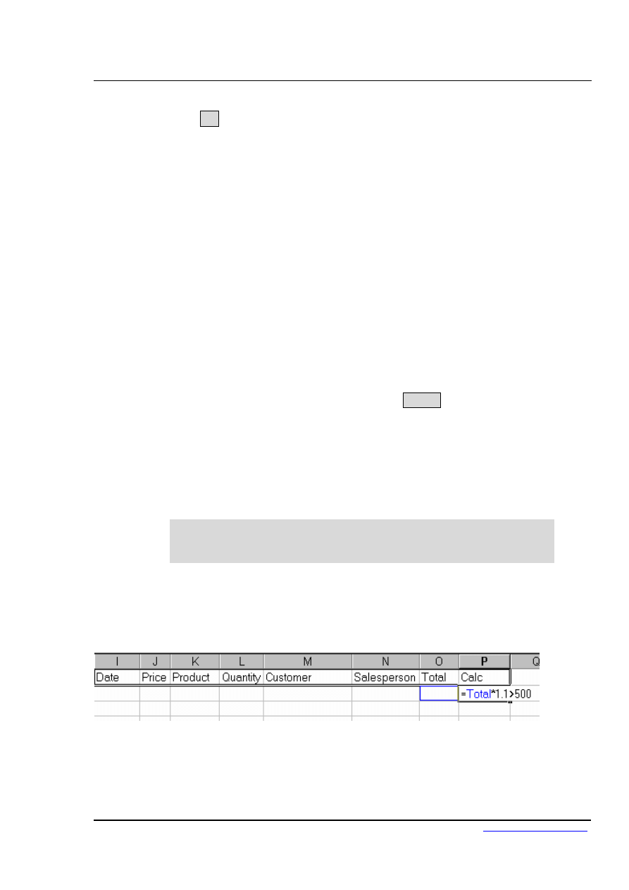
Excel 2002 Advanced Level
Using Excel to Manage Lists
Page
85
Criteria and choose OK. The area covered by that name will be highlighted. You may
choose to alter the selection and redefine the Criteria range again to adjust it.
Calculated Criteria
You may also choose to find data subject to calculated criteria rather than exactly
matching data or using comparison operators or wildcard characters. This would let you
find data that matches the result of a formula, rather than a value that you have entered
directly
To use calculated criteria:
Mouse
1.
Include in the Criteria range one column name which is not used in
the list - Calc for example.
2.
Choose Insert from the menu bar, then Name, Define. Select
Criteria from the names list and click Delete.
3.
Select the column labels (including Calc or whatever you have
named it) plus at least one row below them depending on whether
you need use multiple OR conditions to filter your data.
4.
Choose Insert from the menu bar, then Name, Define. Type
Criteria into the Name box and press [ENTER]
Below the calculated fieldname in the criteria range, you must enter a
formula which refers to the cells contained in the first record of the
database. The formula must result in a TRUE or FALSE answer.
In the example below, in order to find only those records where the value of an order
would increase to over 500 if a 10% increase was applied, the formula shown could be
entered in the Calc column.
When entered, the calculated formula displays on the worksheet as TRUE or FALSE
depending on the figures contained in the first record of the database to which the formula
specifically refers. The underlying formula displays in the formula bar as usual.
© MTC Training Solutions Ltd
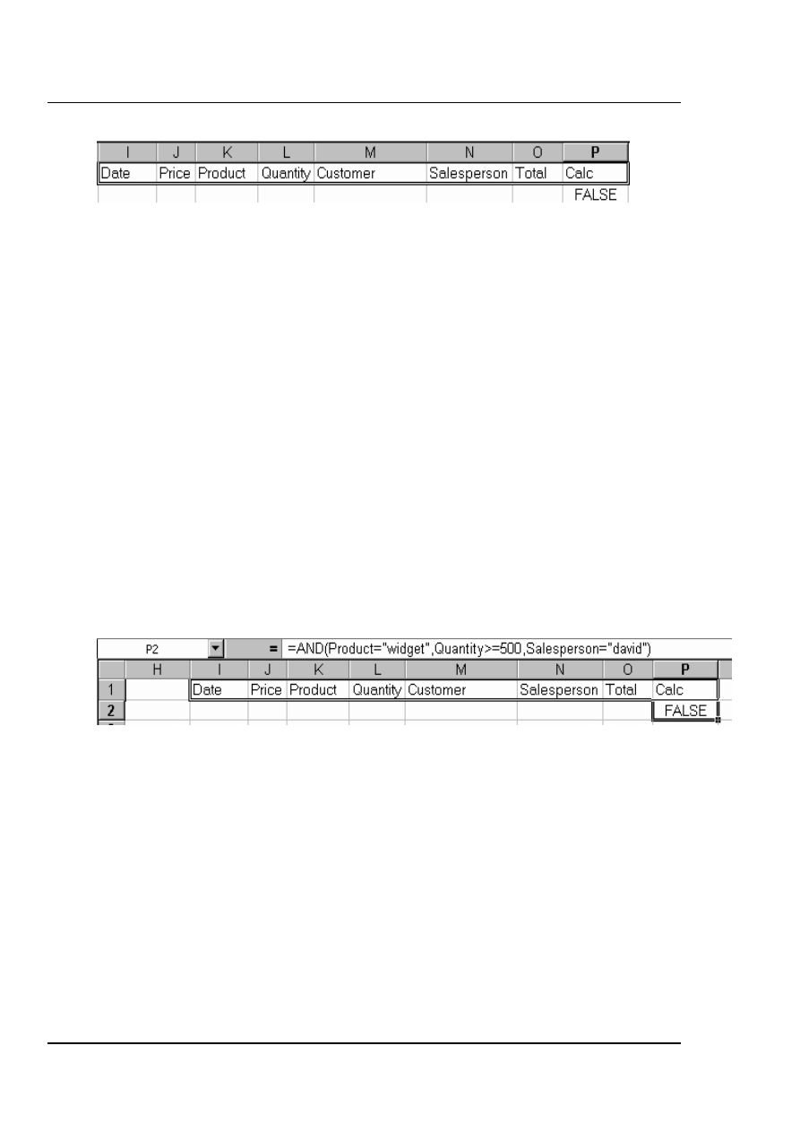
Excel 2002 Advanced Level
Using Excel to Manage Lists
Page
86
You may use calculated fields to refer to and manipulate cells within the first record of
the database, and to refer to cells outside of the database area. For example, the threshold
figure of 500 might be held in an input cell outside the database. If this was the case, that
cell reference could be included in the calculated search criteria, but the reference to it
would need to be absolute or fixed.
Calculated Criteria using Functions
Some of Excel's Logical Functions are particularly suited to setting Criteria for a list
search. Rather than having to extend the criteria range, you can specify criteria as
arguments within the AND(), OR() or NOT() functions.
=AND()
If there are several specifications, every one of which must be met by all records found,
use the AND() function and refer once again to the cells contained in the first record of
the database. Text entries must be enclosed in double quotes. The AND() function may
contain up to 30 comma separated arguments
Referring to the database in the diagram below, for example, if the Quantity must be
greater than or equal to 500, the Product a Widget and the Salesperson David, the
calculated function might be set as appears on the Formula bar:
© MTC Training Solutions Ltd
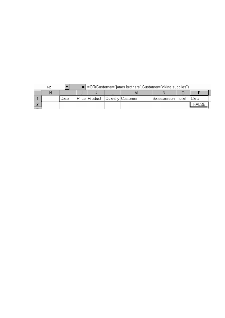
Excel 2002 Advanced Level
Using Excel to Manage Lists
Page
87
=OR()
Searching for two different entries in the same field would necessitate the use of the OR()
function. You may wish to locate all the records where the Customer is either Jones
Brothers or Viking Supplies. Obviously the AND() function will be inappropriate,
because the customer cannot be both companies simultaneously. Instead, the calculation
might be:
Excel will find any records where any one of the arguments contained in the OR()
function is met. The OR() function may contain up to 30 comma separated logical
arguments.
=NOT()
The NOT() function can be used to exclude records meeting certain criteria from the find
operation. Entering a calculation such as:
=NOT(product="Gimlet")
will allow Excel to find all those records where the Product is anything other than a
Gimlet. The NOT() function contains only one argument. It can be combined with other
functions, for example:
=AND(NOT(product="Gimlet"),quantity<20)
will find all those orders for items other than Gimlets where the Quantity ordered was less
than 20.
© MTC Training Solutions Ltd

Excel 2002 Advanced Level
Using Excel to Manage Lists
Page
88
Copying filtered data
You can use the Data, Filter, Advanced Filter command to copy the sets of data that meet
the criteria in the Criteria range to another location on the worksheet.
To copy filtered data to another location:
Mouse
1.
Set the Criteria range.
2.
Place the active cell within the list.
3.
Choose Data from the menu bar, then Filter, Advanced Filter.
4.
In the resulting dialog box, choose Copy to Another Location.
5.
In the Copy To text box, enter a worksheet cell that represents the
top left-hand corner of where you would like the results.
6.
Click OK.
Data copied
to here
If you want to copy only certain columns from the matching sets of data,
enter the column labels exactly as they appear in the list in the location
you want to copy to. When you run the filter, set the Copy To range
reference to the cells where you have typed the column labels.
© MTC Training Solutions Ltd

Excel 2002 Advanced Level
Using Excel to Manage Lists
Page
89
© MTC Training Solutions Ltd
Unique
There is a check box [ ] allowing you to select Unique records only. This may be useful
if, for example, the Copy To range does not include all the column labels. There may be
several records where the Product and Customer are the same. If the Quantity, Date and
Salesperson are not included in the Copy To range, this could result in several seemingly
identical records being extracted. Checking the Unique records only check box before
choosing OK would result in Excel extracting only the first record in each instance.

Excel 2002 Advanced Level
Using Excel to Manage Lists
Page
90
© MTC Training Solutions Ltd
List Statistics
There are several Excel functions which are specifically designed to enable you to
analyse database information. A selection of these appear in the table below.
Database Functions
Function Purpose
DCOUNT(Database,Field,Criteria)
To count the number of records in a list
which meet specified criteria. This
function will only count value cells.
DCOUNTA(Database,Field,Criteria)
To count the number of records in a list
which meet specified criteria. This
function includes text and value cells.
DSUM(Database,Field,Criteria)
To add the contents of the chosen field in
a list, subject to any specified criteria.
DMIN(Database,Field,Criteria)
To find the minimum value in the chosen
field in a list, subject to any specified
criteria.
DMAX(Database,Field,Criteria) To
find the maximum value in the chosen
field in a list, subject to any specified
criteria.
DAVERAGE(Database,Field,Criteria)
To find the average value of the chosen
field in a list, subject to any specified
criteria.
DGET(Database,Field,Criteria) To
return the contents of the chosen field
subject to any specified criteria. This
function is only valid where a single record
meets the criteria set.
DPRODUCT(Database,Field,Criteria) To
multiply the contents of the chosen
field in a list, subject to any specified
criteria.
In all cases, if the Criteria range is blank, these functions will apply to the entire list area.
Once data is entered in the Criteria range, the results of the Database functions will adjust
to reflect only those records meeting the criteria.
The arguments for all of these functions are identical, and the easiest way to incorporate
them into a worksheet is by using the Paste Function dialog.
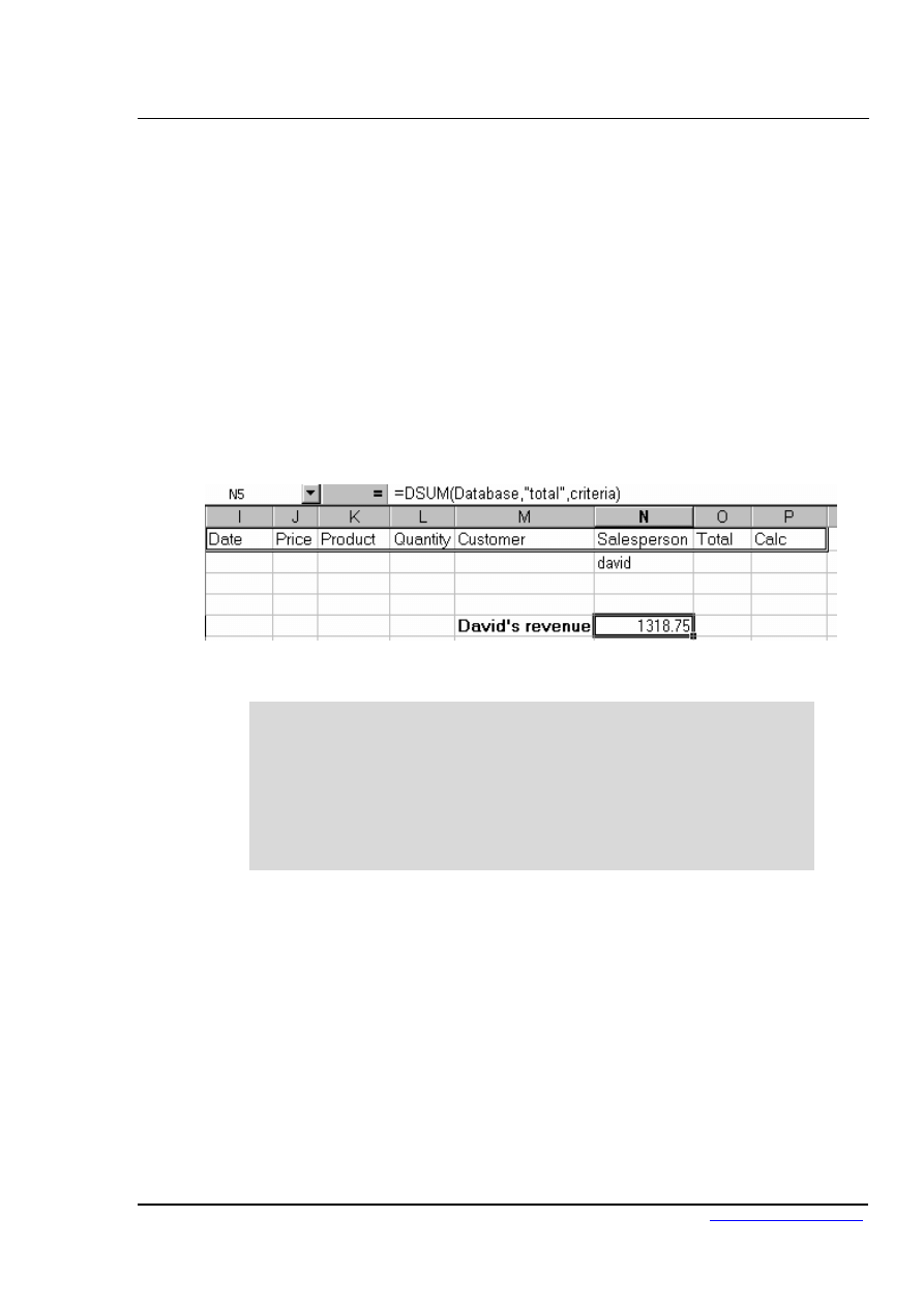
Excel 2002 Advanced Level
Using Excel to Manage Lists
Page
91
To enter a database function on the worksheet:
Mouse
1.
Click the Function Wizard button from the standard toolbar.
2.
In the function category list, select Database.
3.
From the function name list choose the database function you
require: e.g.=DMAX()
4.
Enter the three arguments, list range, field name and criteria range.
5.
Press [ENTER]
If you have assigned the range name Database to your list area and
Criteria to your criteria range you use [F3] to paste the names in.
The field may be entered as a number or as text. Obviously, if the field on
which the function is to operate is the fifth column within the database, you
could enter the number 5 as the field argument. Alternatively, the field
name could be entered as text, in which case it would need to be enclosed
in double quotes:
=DMAX(database,"Price",criteria)
In the above example, the formula shown on the formula bar above has been entered into
the cell to the right of the label “David’s revenue”. This formula sums the total column
ut only where the order was placed through the salesperson David. All the database
nctions look at what has been entered in the criteria range in order to give their results.
b
fu
© MTC Training Solutions Ltd

Excel 2002 Advanced Level
Using Excel to Manage Lists
Page
92
Pivot Tables
A pivot table can summarise large amounts of data using specified calculations and
formats. It is called a pivot table because the headings can be rotated around the data to
view or summarise it in different ways.
The source data can be:
• An Excel worksheet database/list or any range that has labelled columns.
• A collection of ranges to be consolidated. The ranges must contain both labelled rows
and columns.
• A database file created in an external application such as Access or Dbase.
The data in a pivot table cannot be changed as it is the summary of other data. The data
itself can be changed and the pivot table recalculated. The pivot table can be reformatted.
To create a pivot table:
Mouse
1.
Select a cell within your list.
2.
Choose Data from the menu bar, then PivotTable and Pivot Chart
report.
3.
Choose Microsoft Excel List or Database.
© MTC Training Solutions Ltd
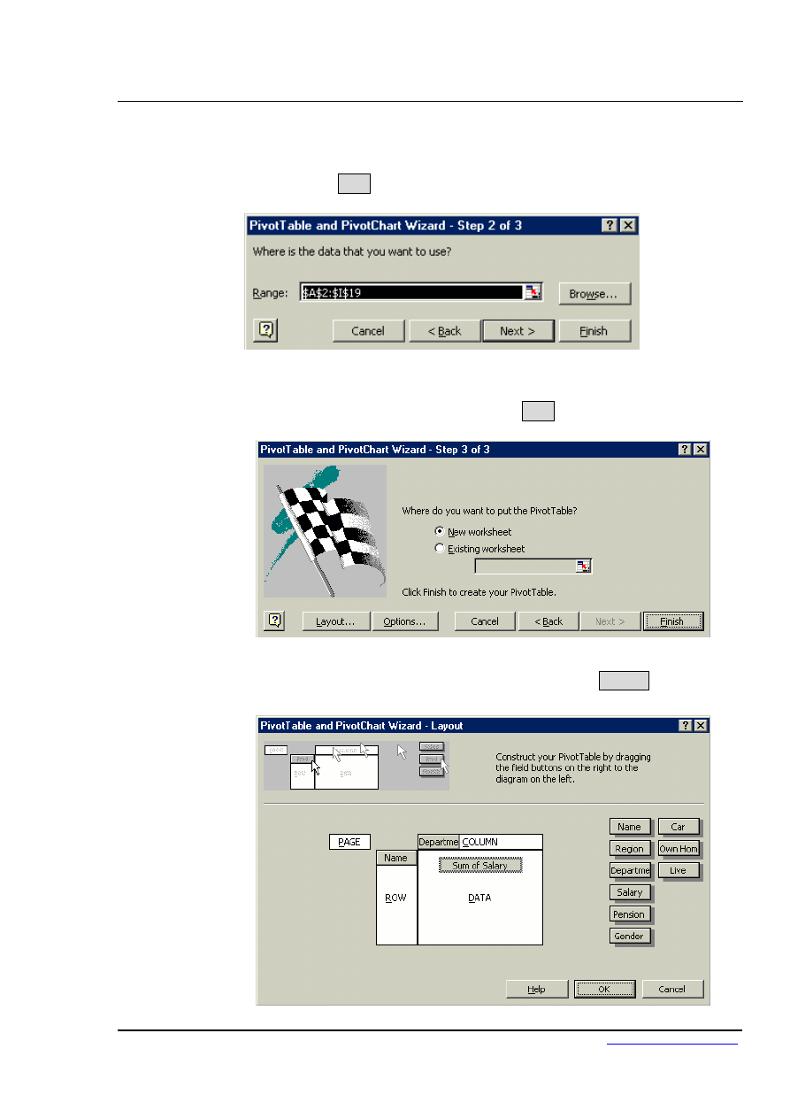
Excel 2002 Advanced Level
Using Excel to Manage Lists
Page
93
4.
Choose Pivot Table
5.
Choose the Next button to go to step 2 of the wizard.
6.
This step verifies where your list data is. Provided the active cell
was within your list when you launched the pivot table wizard, the
worksheet range will be your list. Click Next.
7.
Step 3 is where your will select the destination for you Pivot Table
and decide on the layout of the your Table. Click on Layout.
© MTC Training Solutions Ltd

Excel 2002 Advanced Level
Using Excel to Manage Lists
Page
94
8.
This screen will enable you to define your Pivot Table. A list of
column labels will appear to the right of the screen. Drag and drop
the field buttons for the ROWS, COLUMNS and PAGE labels.
Each row, column or page can have more than one label.
9.
Drag column labels to the DATA area for the fields to summarise.
Excel assumes SUM as the calculation method for numeric fields
and COUNT for non-numeric fields. You can change the
calculation method by double-clicking the field in the DATA area.
10.
Format your summary field in the DATA area by double-clicking it
and choosing Number. Click OK, and then Click OK on the
Layout screen.
11.
Select a destination for your pivot table and click Finish
Managing pivot tables
When data is changed in the pivot table source list, the pivot table does not automatically
recalculate.
© MTC Training Solutions Ltd

Excel 2002 Advanced Level
Using Excel to Manage Lists
Page
95
To refresh a pivot table:
Mouse
1.
Select any cell in the pivot table to be refreshed.
2.
Choose Data from the menu bar, Refresh
Or
Click the refresh button on the Pivot table toolbar
Modifying a pivot table
Adding or deleting fields can modify a pivot table.
To modify a pivot table:
Mouse
1.
Select any cell in the pivot table to be modified.
2.
Choose Data from the menu bar, then PivotTable or click the Pivot
Table Wizard button on the Pivot table toolbar, then click on
layout.
To swap pivot table row and column headings:
Mouse
1.
Using the Pivot Table Toolbar, drag and drop the column or row
headings on and off the Pivot Table
Changing the data that appears in the pivot table:
1.
Click on the down arrow next to the column or row headings
within the pivot table
© MTC Training Solutions Ltd
2.
From the drop down box uncheck the data that you do not want
shown, click on OK

Excel 2002 Advanced Level
Using Excel to Manage Lists
Page
96
© MTC Training Solutions Ltd
Grouping pivot table items
Data can be summarised into higher level categories by grouping items within pivot table
fields. Depending on the data in the field there are three ways to group items:
• Group selected items into specified categories.
• Automatically group numeric items
• Automatically group dates and times
To group selected items:
Mouse
1.
Select the items to group. Select adjacent items by clicking and
dragging or non-adjacent items by selecting each item whilst
holding [CTRL].
2.
Choose Data from the menu bar, then Group and Outline, Group
To group numeric items into ranges:
Mouse
1.
Select a single item.
2.
Choose Data from the menu bar, then Group and Outline, Group
3.
Excel displays a dialog box in which to enter starting, ending and
interval values. Enter appropriate values
4.
Click OK.
To group a date or time in a range:
Mouse
1.
Select a single item.
2.
Choose Data from the menu bar, then Group and Outline, Group.

Excel 2002 Advanced Level
Using Excel to Manage Lists
Page
97
© MTC Training Solutions Ltd
3.
Excel displays a dialog box in which to enter starting, ending and
interval values.
4.
Enter appropriate values and click OK.
Creating a Pivot Table Chart
Mouse
1.
Select a cell within your list.
2.
Choose Data from the menu bar, then PivotTable and Pivot Chart
report.
3.
Choose Microsoft Excel List or Database.
4.
Choose PivotChart (with Pivot Table), click on Next
5.
Follow though the steps as before click on Finish
6.
A chart sheet will appear displaying your Chart
7.
All of the modifying features work in the same way as a standard
pivot table.
8.
To change the format of the chart see Section Four

Excel 2002 Advanced Level
Using Excel to Manage Lists
Page
98
© MTC Training Solutions Ltd
☺
Useful Information
If you are experiencing problems analysing list data check the following:-
•
Your list is correctly set up with the first row containing the column labels identifying
data in each of the columns and no blank rows between the headings and the first row
of data.
•
Your column headings are not ambiguous - ie they cannot be confused with function
names or range names.
•
Your column headings are formatted to make them stand out from the data.
•
Your column headings ideally should not contain spaces - you can remove the spaces
completely or replace them with an underscore (_) character.
•
Your criteria range should only contain a row of headings and blank rows below. The
headings must exactly match the headings at the top of your list.
•
Problems sometimes occur if the criteria range looks blank but perhaps has a space in
it.

Excel 2002 Advanced Level
Using Excel to Manage Lists
Page
99
© MTC Training Solutions Ltd
.
Notes

Excel 2002 Advanced Level
Charts
Page
100
© MTC Training Solutions Ltd
Section 4
Charts
Objectives
By the end of this section you will be able to:
Create embedded charts
Create separate page charts
Change chart types and formats
Add and remove chart data
Add trend lines to charts
Create picture charts
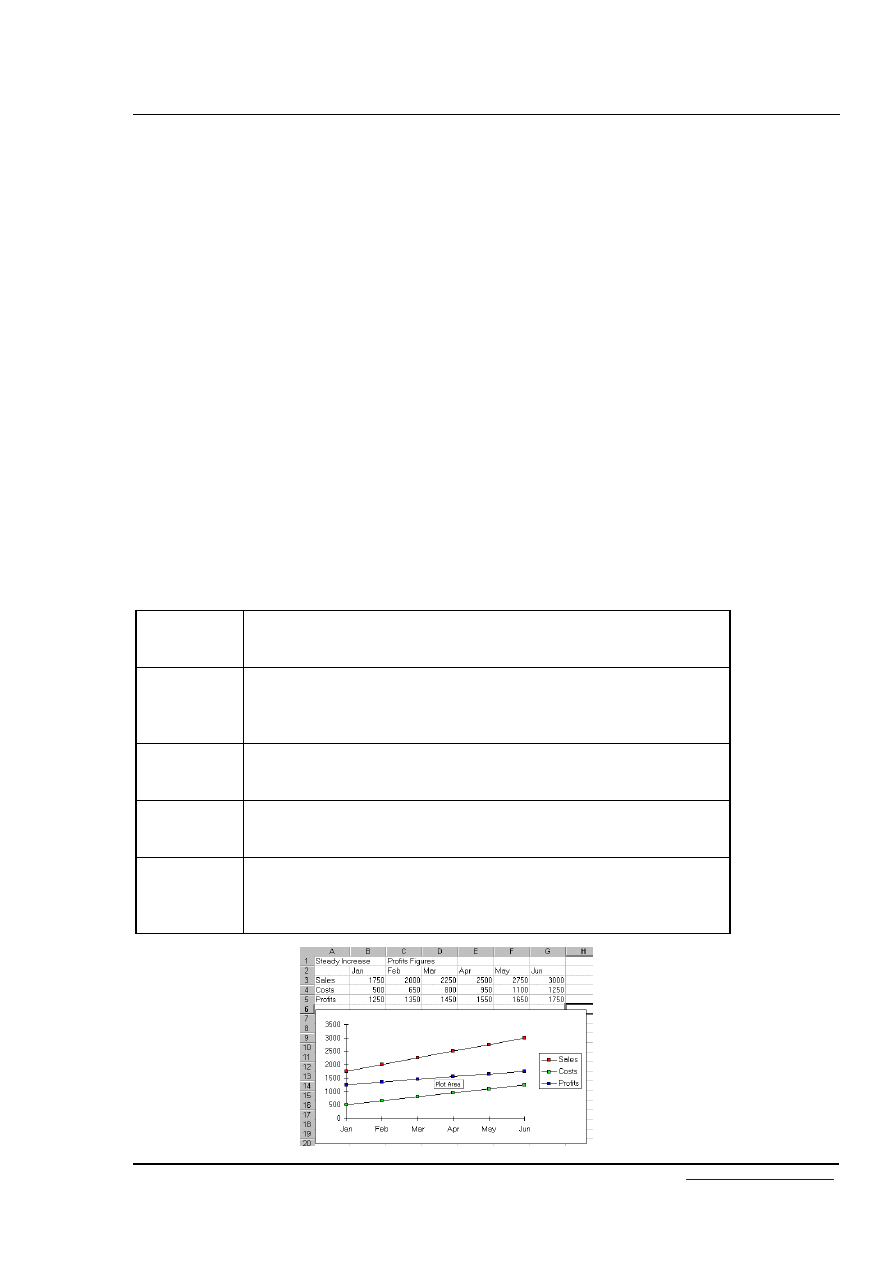
Excel 2002 Advanced Level
Charts
Page
101
Introduction to Charting
One of the most impressive aspects of Excel is its charting ability. There are endless
variations available, allowing you to produce a chart, edit and format it, include notes,
arrows, titles and various other extras as desired. This manual will look at many of the
issues involved in producing and formatting Excel charts.
Charts are based on data contained in Excel Worksheets. It is necessary to understand
how Excel picks up the data to be used in a chart because the way in which the data is laid
out will influence how the chart is presented.
Terminology
As a starting point, there are some terms used in charting which should be understood by
you. The terms defined below relate to the example car sales worksheet and column chart
which appear beneath the table:
Data Point
An individual figure on the spreadsheet which is reflected in the
chart e.g. Fred's Orion sales figure
Data Series
A collection of related data points, e.g. all of Fred's figures,
which will appear on a chart as markers (bars, for example) of
the same colour
Legend
The "key" to the chart, identifying which patterns/colours relate
to which data series
Marker
A bar, column, or slice of pie for example, representing a data
point
Category
The category axis appears across the bottom of a graph (pie
charts excepted) and the categories are listed here. Points
within the different data series are grouped by category
© MTC Training Solutions Ltd

Excel 2002 Advanced Level
Charts
Page
102
© MTC Training Solutions Ltd
Excel Charts
Excel offers a wide range of types and formats from which you can choose when
producing charts. However, the charts themselves can exist in different forms and it is
important to understand the difference between them. The first form is an embedded
chart, the second is a separate chart page.
Embedded Charts
An embedded chart appears on the worksheet where it was created. It is an embedded
object, which does not normally appear in its own window, and has no separate existence
apart from the worksheet. The chart is saved only when the worksheet file itself is saved,
and will be printed with the worksheet in which it is embedded. The Chart Wizard will
ask you whether you want an embedded or separate chart when you first create one.
Separate Chart Pages
A chart sheet, although linked to the worksheet whose figures it represents, exists as a
separate page in a workbook.

Excel 2002 Advanced Level
Charts
Page
103
© MTC Training Solutions Ltd
ChartWizard
Excel has a 4-step process for creating a chart, called the ChartWizard. Each step
explains what you are supposed to do at each stage. The steps are as follows:
• Choose the type of chart
• Check that you have selected the correct data
• Choose the Chart Options required, i.e. labels, title or legend
• Choose whether you want the chart on a new sheet or as an object in a sheet
To create a chart using the wizard:
Mouse
1.
Before proceeding with the above steps you should select the data
you want to chart. When selecting this data, you must include at
least one series of numbers. You may also wish to include text
headings above and/or alongside your figures as it may be helpful
to see these on the chart. The following illustration depicts a
typical selection for charting.
2.
Click on the ChartWizard button on the Standard toolbar – the
ChartWizard dialog will open and guide you through the four steps
of the ChartWizard.
3.
Step 1 – choose the type of chart required. Use the Press and hold
to view sample button to see what the chart will look like. Click
Next to move to Step 2.
4.
Step 2 – specify the data to be plotted on the chart – these will be
the cells you selected before launching the Chart Wizard. If you
have changed your mind and no need to include extra cells, you
can select them now by clicking in the Data Range text box. Click
Next to move to the next step.
5.
Step 3 – change the way the data in the chart looks. This is where
you can turn on and off some of the standard options for the chart
type you selected.

Excel 2002 Advanced Level
Charts
Page
104
© MTC Training Solutions Ltd
Chart Element
Description
Titles
This is the area where you can specify the
titles to have on the chart (i.e. X-axis “1998”,
Z-axis “GBP”
Axes
Here you specify whether you want a Y/Z
axis and whether you are using timescales to
plot your data
Gridlines
The gridline tab allows you to switch on and
off horizontal and vertical gridlines
Legend
Use this tab to switch the legend on and off
or reposition it
Data Labels
The Data Labels tab allows you to display the
amount each point represents or display the
label (i.e. in the example above, each
cylinder would have Qtr1, Qtr2 displayed as
appropriate at the top of each data marker)
Data Table
The Data Table tab will display a grid
underneath the chart that will show the
information that is being plotted.
Make your choices and click Next.
6.
The final step allows you to add the chart either as a new chart
sheet or as an embedded object that will print alongside the data it
represents. Make your choice and click Finish.
Moving and resizing embedded charts
Once the chart object has been created and stored as an embedded object, you can move
and resize it.
To move an embedded chart:
Mouse
1.
Click just inside the chart frame border and hold the mouse button
down as you drag. Release the mouse when the chart is in the
desired location.

Excel 2002 Advanced Level
Charts
Page
105
© MTC Training Solutions Ltd
To resize an embedded chart:
Mouse
1.
Click just inside the Chart frame border.
2.
Position the mouse over one of the handles provided at the object’s
corners.
3.
Drag up, down, left or right.
Hold down the [ALT] key if you wish the chart to resize by snapping to the
cell gridlines
Creating Separate Chart Pages
The wizard will offer you the option of creating an embedded or a separate page chart,
however, there is a very quick way of producing a separate page chart using Excel’s
default chart settings.
To create a separate chart file:
Keyboard
1.
Select the data to be charted, including row and column headings
2.
Tap the [F11] function key.
This technique will result in a chart window appearing on screen, reflecting the worksheet
data which was selected. The default graph settings are for a 2-dimensional column chart.

Excel 2002 Advanced Level
Charts
Page
106
Data Layout
Depending on the "shape" of the selected data, Excel will assign categories and data
series to either the rows or columns of information. Usually it will be assumed that there
are more categories than data series, therefore, if there are more rows than columns of
selected information, the data series will be based on columns, with the legend labels
being picked up from the row across the top of the selected area and the category labels
being picked up from the leftmost column:
0
500
1000
1500
2000
2500
3000
3500
Jan
Feb
Mar
Apr
May
Jun
Sales
Costs
Profits
If there are more columns than rows in the selected area, the data series will be based on
rows, with the legend labels being picked up from the leftmost column and the category
labels taken from the top row of the selected area:
© MTC Training Solutions Ltd
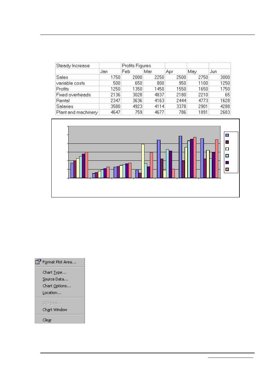
Excel 2002 Advanced Level
Charts
Page
107
0
1000
2000
3000
4000
5000
6000
Sales
variable
costs
Profits
Fixed
overheads
Rental
Salaries
Plant and
machinery
Jan
Feb
Mar
Apr
May
Jun
If the number of rows and columns is the same, Excel will opt for data series in rows. It
is possible to override the choice made by Excel in how the data series and categories are
decided. Details of this procedure will be found under the section on manipulating data.
Shortcut Menus
You may be familiar with the Shortcut menus associated with the selected cell(s) on the
Excel worksheet. When working on a chart - either embedded on a worksheet or in its
own window, clicking on the chart with the secondary mouse button will call up a
Charting Shortcut menu.
The Shortcut menu will contain a selection of choices from some of
the Standard Menu bar options mostly relating to the chart as an
embedded object - almost like a graphic on the worksheet.
© MTC Training Solutions Ltd
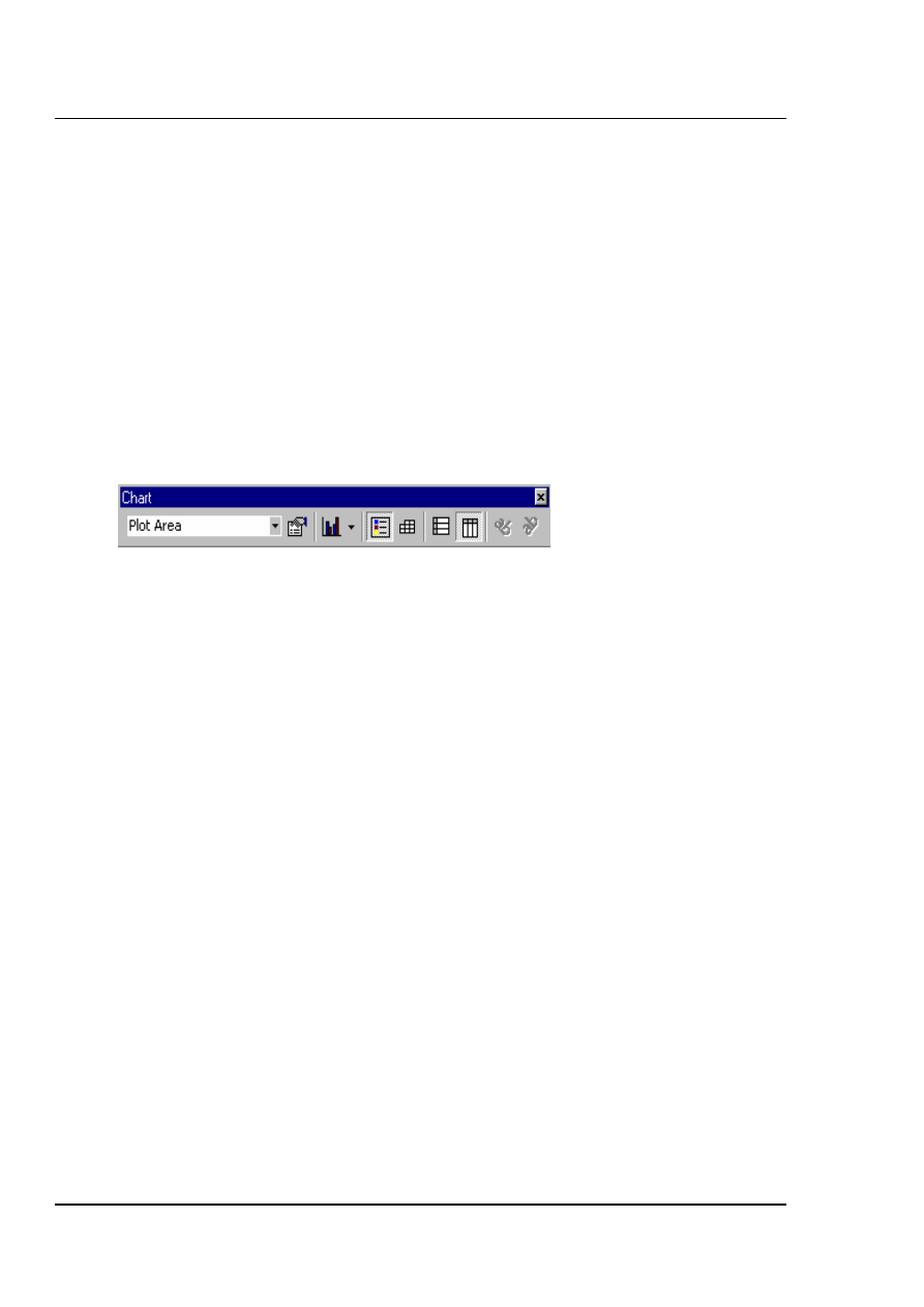
Excel 2002 Advanced Level
Charts
Page
108
Chart Toolbar
There is a Chart toolbar in Excel which includes tools for many of the most commonly
accessed charting options. The toolbar will usually appear on screen automatically when
a chart (either embedded or separate) is active. When dealing with an embedded chart,
you may find that the Chart toolbar vanishes if an area on the worksheet is selected, then
reappears when the chart is selected.
If you deliberately hide the Chart toolbar while the chart is selected, it will no longer
appear automatically on selecting the chart.
© MTC Training Solutions Ltd

Excel 2002 Advanced Level
Charts
Page
109
Chart Types
There are several different types of chart available within Excel. The type to choose will
vary depending on the data involved and what information the chart is intended to convey
or highlight. Practice will improve your instinct on which type of chart to use in each
instance. Initially it may be useful to try different types until the result is reasonably
close to your requirements, and then add custom formats and elements as desired. Some
chart types are very specialised and may only be of use to particular business sectors.
Available types
Click on the Chart button from the chart toolbar to see the chart types
available.
Selecting any of the types listed will apply a given chart type to the active
chart. The most useful types available and some of their applications have
been summarised below:
Area
Area charts can be 2 or 3-dimensional. They are used to compare the change in volume
of a data series over time, emphasising the amount of change rather than the rate of
change. Area charts show clearly how individual data series contribute to make up the
whole volume of information represented in the graph.
Bar
Bar charts can be 2 or 3-Dimensional. They are used to show individual figures at a
specific time or to compare different items. Categories are listed vertically, so that bars
appear on the horizontal, thus there is less emphasis on time flow. Bars extending to the
right represent positive values while those extending left represent negative values.
Column
Column charts can be 2 or 3-Dimensional. They are frequently used to show variation of
different items over a period of time. Categories (often days or months for example,
representing a progression of time) are listed horizontally and columns are displayed side
by side, making for easy comparisons.
Two variations on the theme of Column charts are represented by further tools on the
Chart toolbar. The Stacked Column chart can be used to show variations over a period of
time, but also shows how each data series contributes to the whole. A further variation on
© MTC Training Solutions Ltd

Excel 2002 Advanced Level
Charts
Page
110
© MTC Training Solutions Ltd
the 3-D column chart produces 3-D columns in a 3-D plot area, receding away from the
viewer.
Line
Line charts can be 2 or 3-Dimensional. Line charts are used to compare trends over time.
There are similarities with Area charts, but line charts tend to emphasise the rate of
change rather than volume of change over time. 3-D lines appear as "ribbons" which can
be easier to see on the chart.
Pie
Pie charts can be 2 or 3-Dimensional. They are used to compare the size of the parts with
the whole. Only one data series can be plotted, making up 100%. Pie charts within their
own window can be made to "explode" by dragging one or more pieces of pie away from
the centre.
Radar
Each category in a radar chart has its own axis radiating from the centre point. Data
points are plotted along each spoke, and data points belonging to the same series are
connected by lines.
XY Scatter Charts
XY charts are used to compare two different numeric data series, and can be useful in
determining whether one set of figures might be dependent on the other. They are also
useful if the data on the X axis represents uneven intervals of time or increments of
measurement.
Combination
A combination chart allows you to overlay one 2-Dimensional chart type on top of
another. This can be useful for comparing different types of data, or for charting data
requiring two different axis scales. Once the combination chart has been set up, the
actual type of the main or overlay chart can be changed by you.
3-D Surface
3-D Surface charts present information in an almost topographical layout. They can be
used to pinpoint the high and low points resulting from two changing variables. It can be
helpful to think of a 3-D surface chart as a 3-D Column chart which has had a rubber
sheet stretched over the tops of the columns.
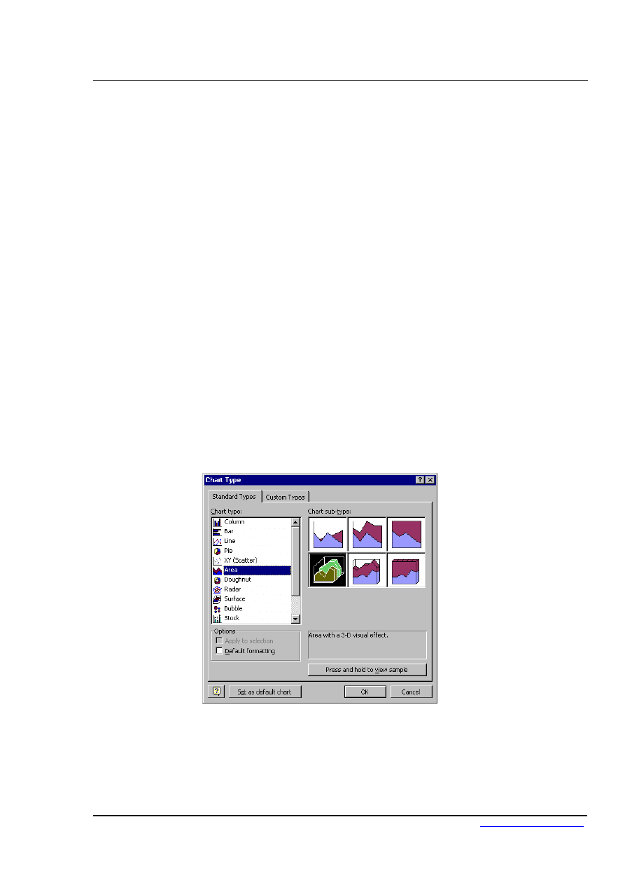
Excel 2002 Advanced Level
Charts
Page
111
To change the chart type:
Mouse
1.
Select the created chart.
2.
Click the chart type button from the Chart toolbar.
3.
Click on the chart that you want to use to plot your data. The
selected type will be applied to your chart.
Default Chart type
The default graph setting in Excel is set to a simple 2-dimensional column chart, however
you can change the default to any of the types offered within the chart type dialog.
To set the default chart type:
Mouse
1.
Choose Chart from the menu bar, then Chart type.
2.
Select the chart type from the list and click on the specific format
that you want the chart to have from the gallery of pictures on the
right.
© MTC Training Solutions Ltd
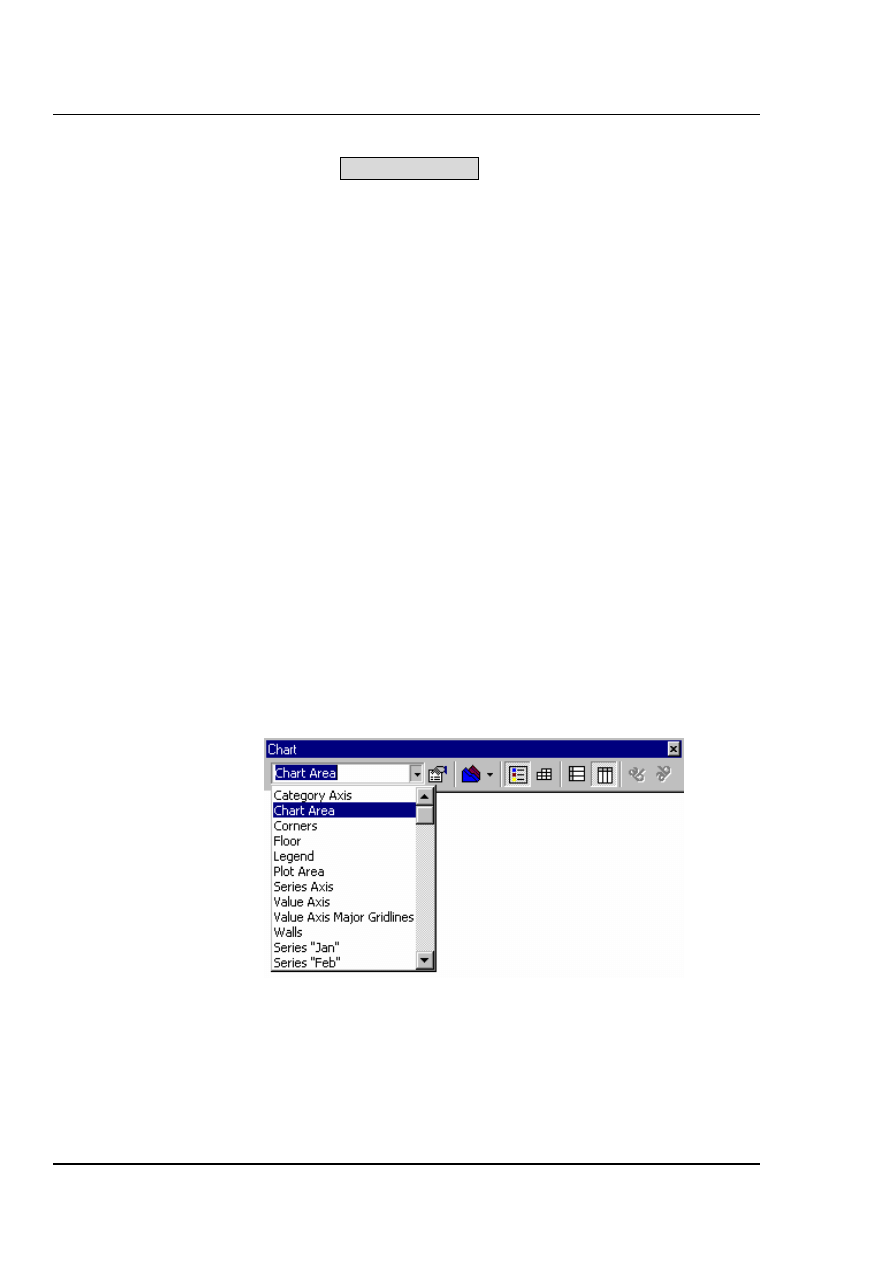
Excel 2002 Advanced Level
Charts
Page
112
3.
Click the Set as default chart button.
New charts created from now on will use the default format as defined by you.
Formatting Charts
There are several different ways of formatting the various elements in a chart. Some
formats, such as adding a legend can be applied to a chart using the Chart toolbar.
Calling up the Shortcut menu on a Chart will also allow you to access the dialog boxes
which can be used to change formatting on the entire chart.
Format chart elements
Your chart is made up of many different elements each of which can be formatted. You
must select the particular element that you want to format prior to changing it.
To select a chart element:
Mouse
1.
Select your chart by clicking on it.
2.
Click the drop-down list arrow to the right of the chart element list
box on the charting toolbar. A list of all the chart elements will
appear.
3.
Click on the element you wish to select.
Format Chart Area
You may choose to add a Border to the chart, or add patterns and shading to its
background.
© MTC Training Solutions Ltd
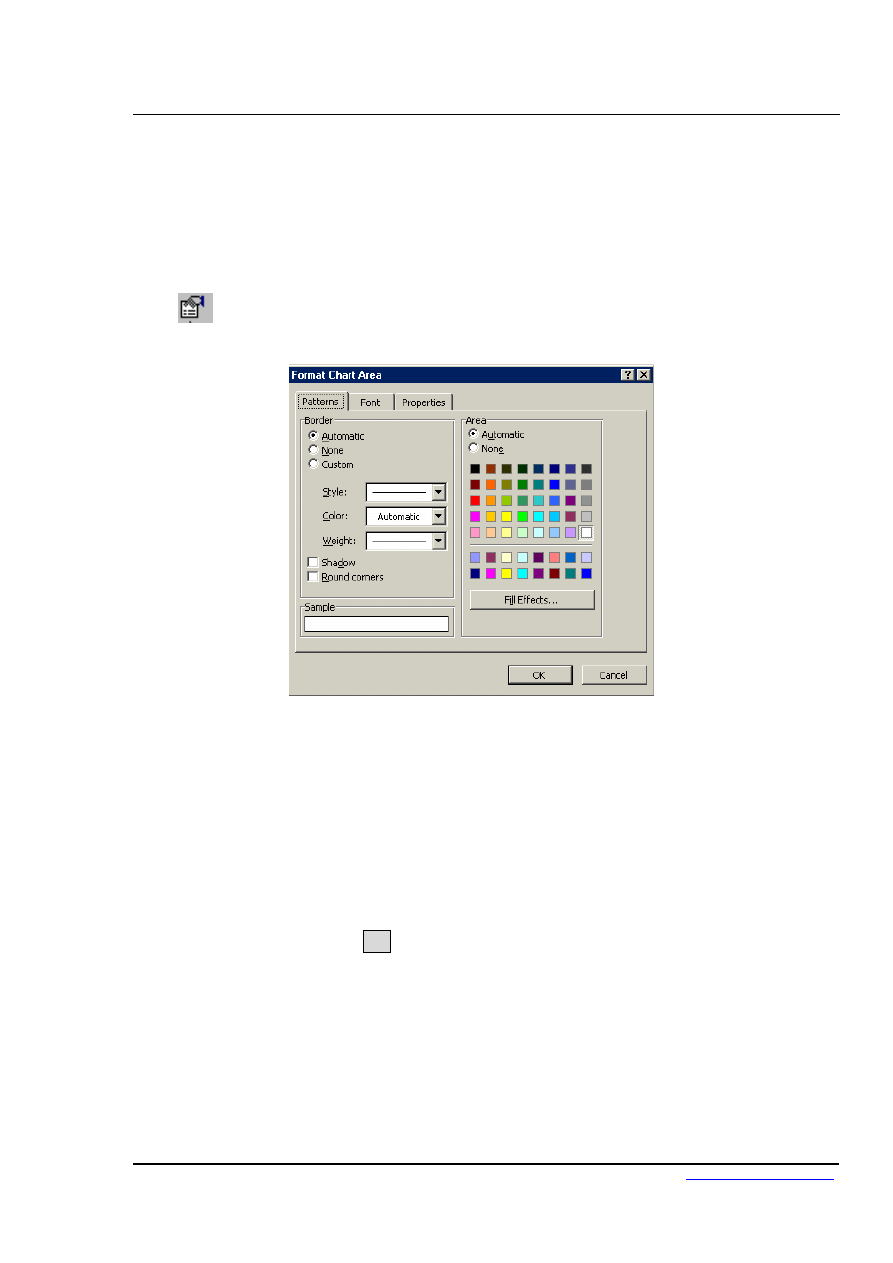
Excel 2002 Advanced Level
Charts
Page
113
To format the chart area:
Mouse
1.
Select the chart area.
2.
Click the Format selected item button from the Chart toolbar. The
following dialog box will appear:
3.
Set the Border option to add a border around the outside of the
chart area.
4.
Use the Area option to specify background colours.
5.
Click the Font tab to set font formatting options for the whole
chart.
6.
Click the Options tab for settings determining how the chart will
move and print.
7.
Click on OK when the desired settings have been selected.
© MTC Training Solutions Ltd
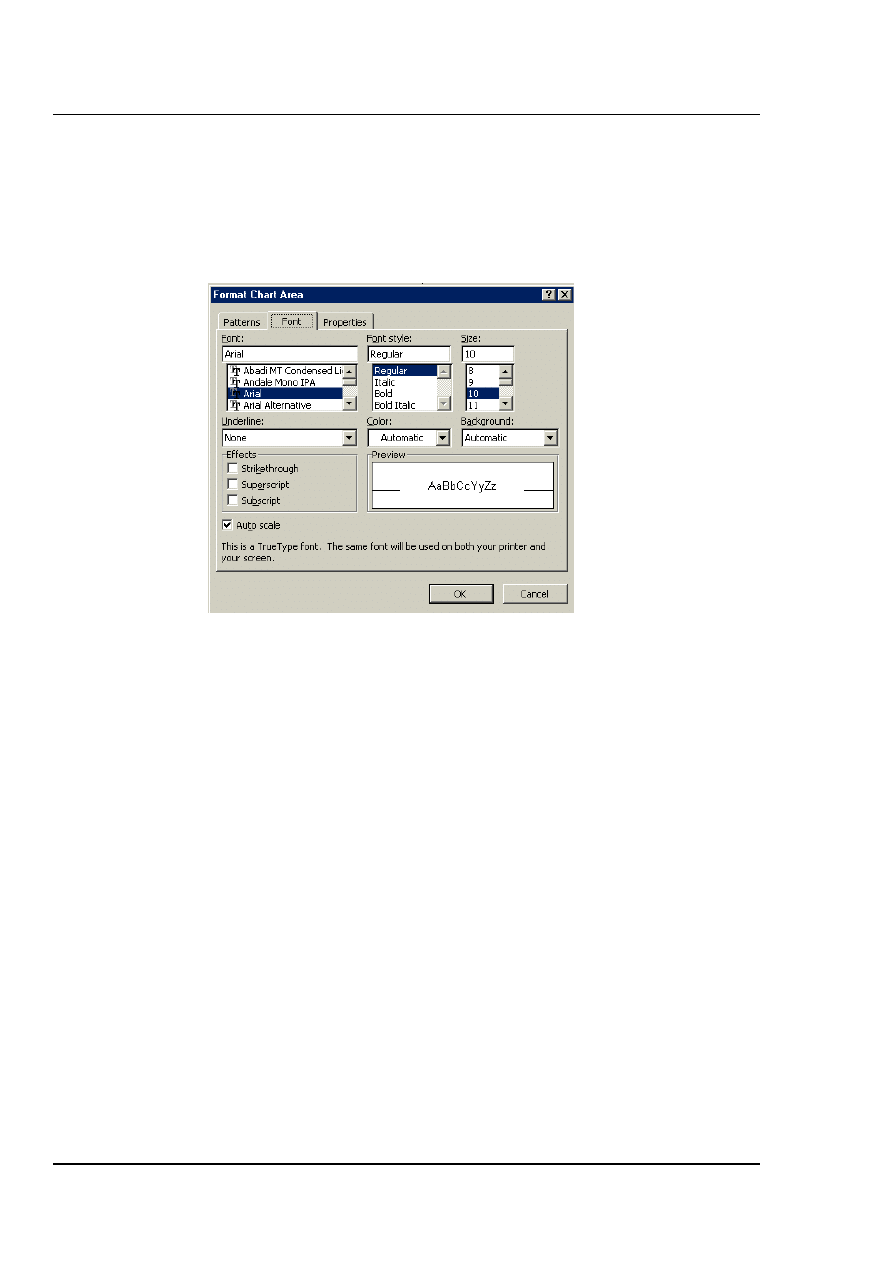
Excel 2002 Advanced Level
Charts
Page
114
Font
From here, you can choose the desired Font for the legend (or other selected text), the
Font Style and the Size.
Special effects such as Strikeout or Underline may be applied to the selected text by
clicking the appropriate Check boxes [ ]. The Colour to be applied to the selected text
may be chosen from a drop down list, and the Sample area will change to reflect the
chosen settings. A further refinement allows you to dictate how the Background behind
the text will appear.
© MTC Training Solutions Ltd
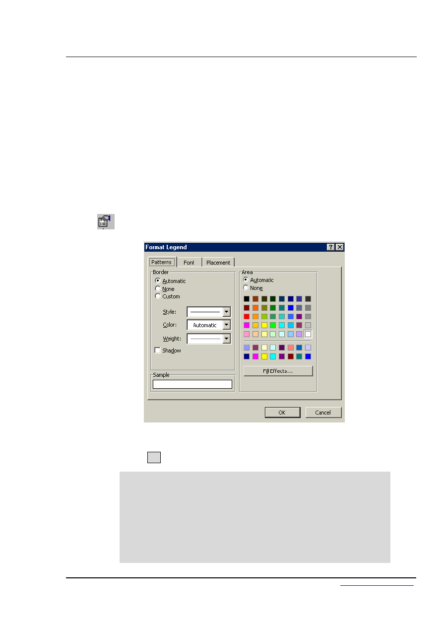
Excel 2002 Advanced Level
Charts
Page
115
Formatting the Legend
The Legend can be selected and formatting like the other chart elements The legend can
be positioned manually simply by pointing and dragging it to a new position on the chart,
but there are some preset positions which can be selected from this dialog box.
To format the legend:
Mouse
1.
Select the Legend.
2.
Click the Format selected item button from the Chart toolbar.
3.
When all the options have been dealt with satisfactorily, click on
OK.
All your selections will now be applied to the legend. Note that the legend
cannot actually be resized. Changing the font size will cause the size of
the overall legend to adjust, but it cannot be resized by dragging on the
selection handles. No chart element which shows white selection handles
(rather than the usual black) can be resized by dragging.
Dragging the legend to a new position on the chart will sometimes affect
the shape of the legend and the size of the chart. The legend may be
placed overlapping the chart, but if it is dragged to the edge of the chart
© MTC Training Solutions Ltd

Excel 2002 Advanced Level
Charts
Page
116
© MTC Training Solutions Ltd
area, thin black lines will appear, indicating that the chart will be moved
aside to make room for the new legend position.
Note that the text appearing in the Legend box is picked up from the
worksheet data. Edit the text on the worksheet in order to change the
legend text (the legend text can also be altered manually - see later section
on Manipulating Chart Data). The legend may be deleted by selecting it
and pressing the Delete key on the keyboard.
Unattached Text
Floating text may be typed directly onto the Chart, then dragged to the desired position.
To add floating text to a chart:
Mouse
1.
With your chart selected, type the text you want to see displayed on
it and press [ENTER].
2.
Move the text to the desired location by clicking and dragging it.
Basic Chart Formats
In addition to double clicking in order to edit specific chart elements, you may use the
Chart Options item from the Chart Menu bar to access a variety of formatting options.
To add chart elements:
Mouse
1.
With the chart selected, choose Chart from the menu bar, then
Chart Options.
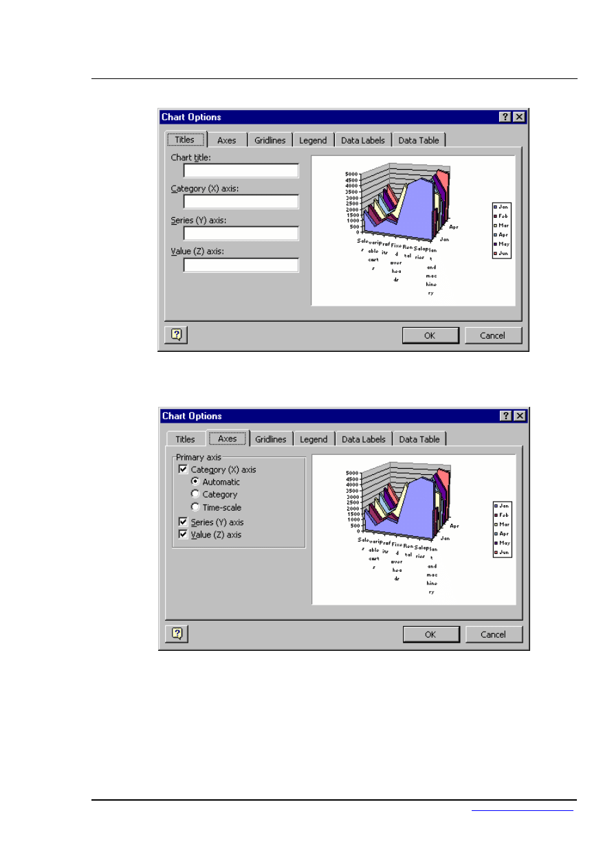
Excel 2002 Advanced Level
Charts
Page
117
2.
Use the Titles tab to specify which titles you want attached to the
chart itself and the various axes.
3.
Use the Axes tab to add or remove axes, or to change the format
of the category axis if you want a timescale.
es
tab to add or remove axes, or to change the format
of the category axis if you want a timescale.
© MTC Training Solutions Ltd
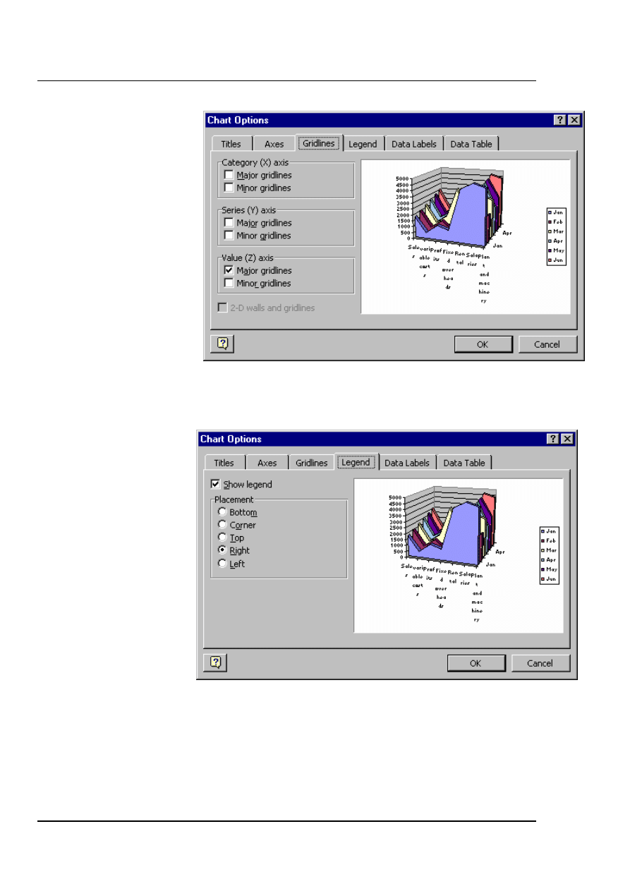
Excel 2002 Advanced Level
Charts
Page
118
4.
Use the Gridlines tab to add the horizontal and/or vertical lines to
your chart. These can be useful in helping you to distinguish the
exact values of the data markers or separate the categories.
5.
Use the Legend tab to switch the Legend on and off and change
its position.
© MTC Training Solutions Ltd
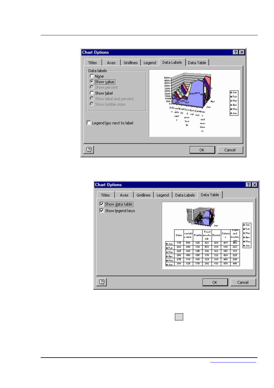
Excel 2002 Advanced Level
Charts
Page
119
6.
Use the Data Labels tab to write the values or the labels on the
data markers.
7.
Use the Data Table tab to add the plot data so that it is visible on
the chart itself.
8.
When all options have been set, click OK.
© MTC Training Solutions Ltd

Excel 2002 Advanced Level
Charts
Page
120
Formatting Axes
The axes can be formatted to appear in different ways, or the scales of the axes can be
changed.
To format the Category (X) Axis:
Mouse
1.
Use the drop-down list of elements on the Chart Toolbar to select
“category axis”.
2.
Click the Format selected chart element button from the Chart
© MTC Training Solutions Ltd
Custom will allow you to define the Style, Colour and Weight of
appear
toolbar. The following dialog box appears:
3.
From the Patterns tab, you can affect the line displayed on the
selected axis. Automatic will apply the default thin black line.
the line. The option for None will suppress the axis from showing.
Under Tick Mark Type, you may click on the appropriate option
button to specify that tick marks on the axis will appear on the
inside or outside of the axis line, cross the axis line, or not
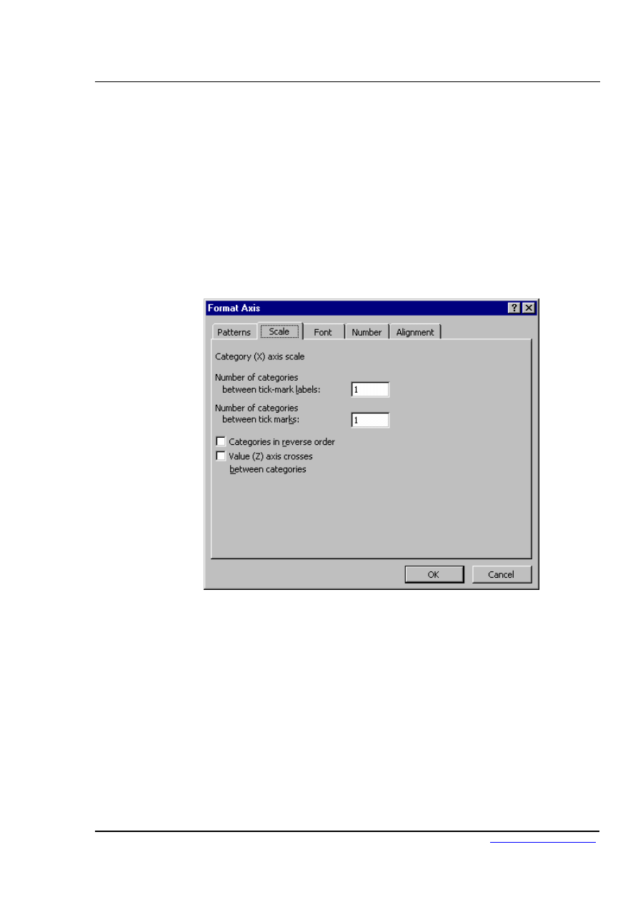
Excel 2002 Advanced Level
Charts
Page
121
© MTC Training Solutions Ltd
u to dictate where the Labels
associated with the selected axis will display. This can be at the
4.
Use the Scale tab to specify at where the value axis will appear,
which categories are labelled, and how many categories will appear
is will also affect the
location of tick marks on the axis. Categories may be displayed in
d to
cross at the last plotted category on the chart.
Font tab to specify font formatting for the axis labels.
at all. Minor tick marks can also be included (click on the Scale...
button to set the intervals for major and minor tick marks).
The Tick Labels section allows yo
High Values end of the axis, the low values end of the axis, next to
the axis, or completely suppressed.
between each pair of tick marks.
A series of check boxes [ ] allows you to dictate whether or not
the Value Axis crosses between categories. The default setting is to
have this box checked, which produces a Value Axis at the edge of
a given category. Unchecking this box will result in a Value Axis
which cuts down the middle of a category. Th
reverse order if desired, and the Value Axis may be require
5.
Use the
6.
Use the Number tab to specify number formatting for the axis
labels.
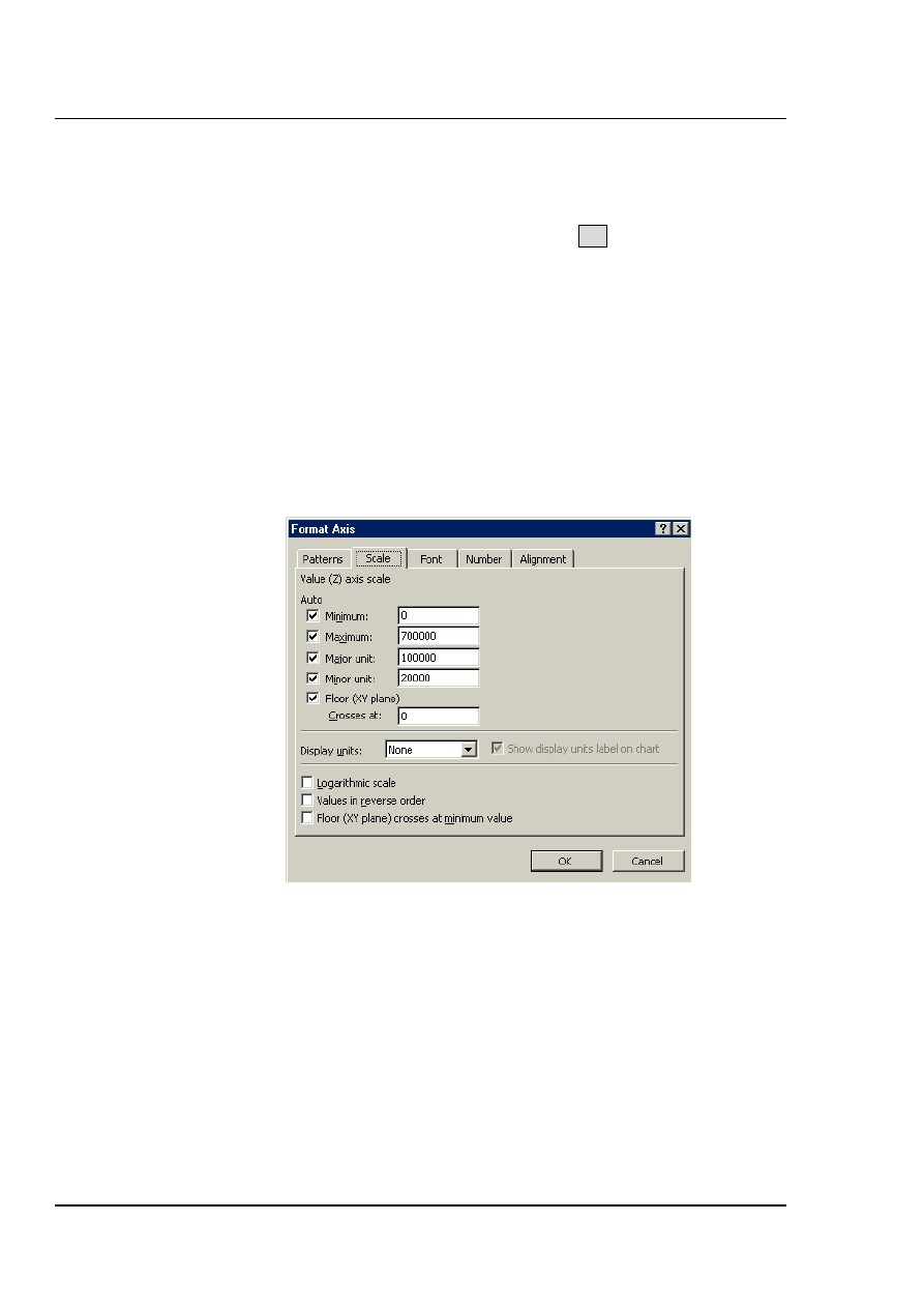
Excel 2002 Advanced Level
Charts
Page
122
7.
Use the Alignment tab to specify the orientation of the category
labels.
8.
When all options have been set, click OK to apply them to your
chart.
t the Value (Y) axis:
eps described above for the category axis.
2.
The Scale tab will have different options relating to the values on
ay also be set. You may dictate the point
at which the value and category axes cross, whether or not the axes
are plotted on a Logarithmic Scale, or whether to have the values
There are several formatting options which are particular to 3-dimensional charts. While
To forma
Mouse
1.
Follow st
the axis.
From the Scale tab, you may specify the Minimum and Maximum
values to appear on the axis. The intervals to be used as Major and
Minor units on the axis m
plotted in Reverse order.
3-D Chart Formatting Options
working on a 3-D chart, many settings can be adjusted by accessing the Format, 3-D
View option from the menu bar.
© MTC Training Solutions Ltd

Excel 2002 Advanced Level
Charts
Page
123
© MTC Training Solutions Ltd
influence the degree of elevation, perspective, or rotation of your
chart. A sample chart within the 3-D view dialog box reflects the new views as you
change these factors.
ping
values into the appropriate sections within the dialog box, or by clicking on the arrow
ple chart. The latter technique is obviously easier.
resents a view level with the centre of
the plot area.
ith 3-D Pie Charts, the range varies from 10°, almost level with the edge of
surface of the pie.
views the chart from the front, 90°would view it from the side, and 180°
would allow you to see it from the back - effectively reversing the order of the data series for
Depending on the data being displayed, some data markers on a 3-D chart may be
obscured. It is possible to adjust the view so that your data may be seen to its best
advantage. You may
Elevation, Rotation and Perspective (if it is available) can be adjusted either by ty
buttons displayed around the sam
Elevation
Elevation dictates the height from which you view the data. Ranging from 90°(above the
plot area) to -90°(below the plot area), where 0° rep
W
the pie, to 80°, looking down on the
Rotation
Rotation allows you to turn the graph on its vertical axis. The range goes from 0° to
360°, where zero
the chart display.
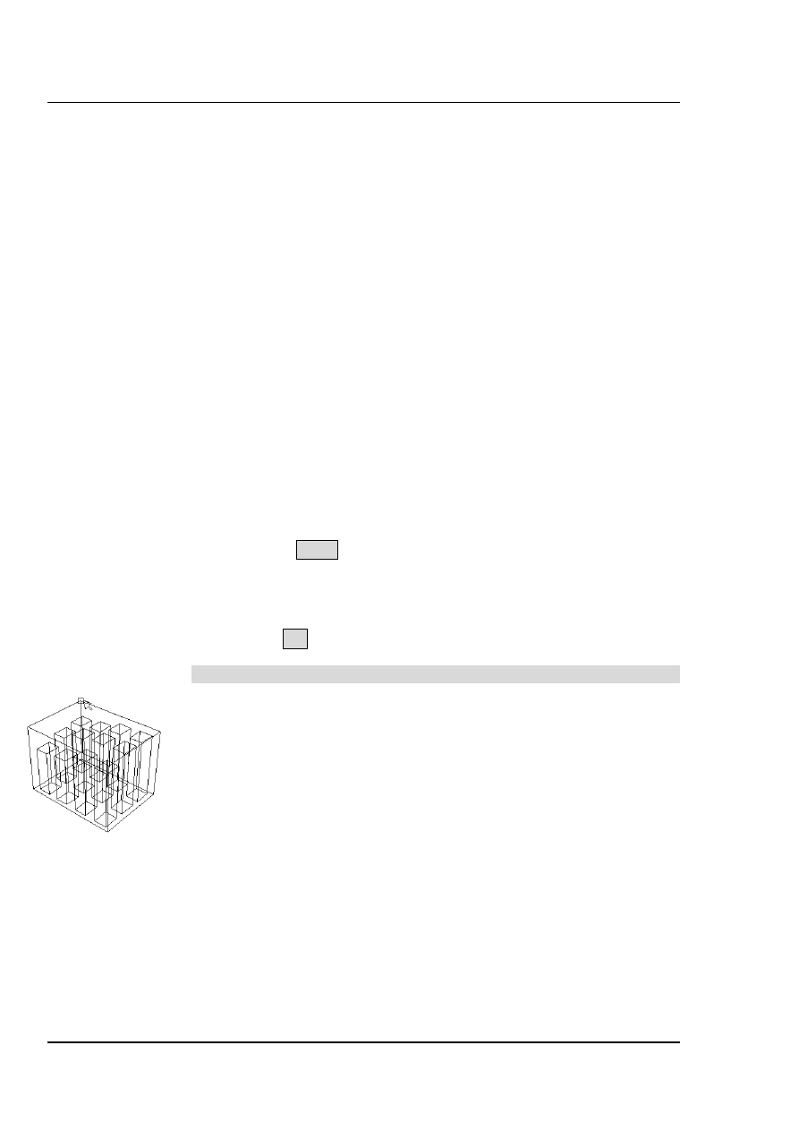
Excel 2002 Advanced Level
Charts
Page
124
Perspective
© MTC Training Solutions Ltd
er.
Yo
also affect the height of the graph in relation to its width and whether or not you
wa
setting would preclude the use of
pe
cale a 3-D chart so that, where
possible, it is sim
size to its 2-D equivalent.
To format the 3-D view:
3-D view.
t the appropriate options.
Perspective can be changed to make the data at the back of a 3-D chart appear more
distant. A perspective of zero means that the farthest edge of the chart will appear as
equal in width to the nearest edge. Increasing perspective (up to a maximum of 100) will
make the farthest edge appear proportionally small
u may
nt the axes to remain at right angles. This latter
rspective in 3-D charts. Auto-scaling allows Excel to s
ilar in
Mouse
1.
Choose Chart from the menu bar, then
2.
Selec
3.
ut keep the
Choose Apply to apply your changes to your chart b
dialog box visible for more changes.
Or
Click OK to close the dialog and apply your changes.
The rotation and elevation of a 3-D chart can also be adjusted manually.
o adju
rea should display the
word "Corners"). Black selection handles should now appear.
2.
Drag one of the selection handles to a new position. Excel will
display a 3-D framework indicating the new chart aspect. Release
when the desired display has been achieved.
T
st rotation and elevation manually:
Mouse
1.
Select any corner of the chart (the reference a

Excel 2002 Advanced Level
Charts
Page
125
© MTC Training Solutions Ltd
Manipulating Chart Data
Delete a Series Manually
It is possible to delete a series from a chart simply by selecting it, then pressing the delete
key.
To delete a data series:
Keyboard
1.
Select the series you wish to delete.
2.
Press [DELETE].
Add a Series Manually
A series may be added to a chart
To add a new data series to a chart:
Mouse
1.
Select the worksheet cells containing the relevant data (including
the label to be used if labels were included in the original data).
2.
Copy this data to the clipboard in the usual way.
3.
Activate the chart by clicking on it and choose Edit, Paste. The
data series will appear in the chart.
The added series will invariably come in as the final data series, but the
order can be changed by you as outlined under Edit Series - Plot Order
later in this document.

Excel 2002 Advanced Level
Charts
Page
126
© MTC Training Solutions Ltd
The Series Function
If a data series on a chart is selected, the reference area will display the underlying
formula. It can be useful to know what elements go to make up the Series function, as
you may edit it manually if desired. The Series function includes four arguments:
=SERIES(Series_Name,Categories_Ref,Values_Ref,Plot_Order)
The Series Name can be a reference (Worksheet!Cell) to the cell where the name of this
particular data series is being held, or it may consist of text typed in by you and enclosed
in quotation marks. The Series Name will be picked up in the legend to describe the data
series.
The Categories Reference refers to the worksheet name and range of cells where the
Category (or x-axis) labels are to be found. If the data series are in rows, the category
references will refer to the labels at the top of each column and vice versa.
The Values Reference refers to the worksheet name and the range of cells containing the
actual values for this data series which are to be plotted on the y-axis (or z-axis on a 3-D
chart).
The Plot Order number dictates the order in which the selected data series is plotted on
the chart and listed on the legend.
Often, instead of amending the Series function manually, you may find it easier to edit a
data series using the menu option covered in the next section.
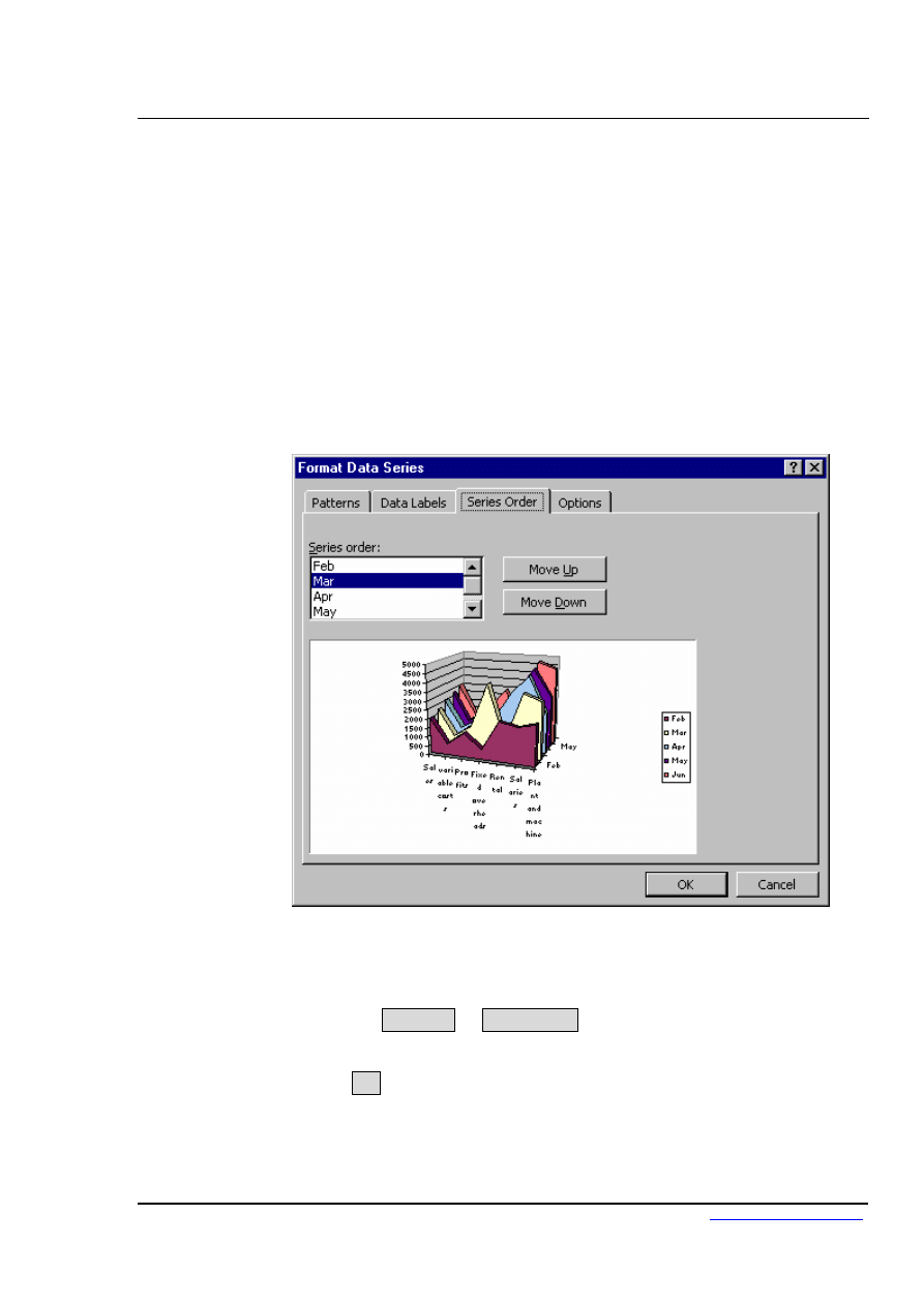
Excel 2002 Advanced Level
Charts
Page
127
Chart, Edit Series
To change a series plot order:
Mouse
1.
Select any series on the chart
2.
Click the Format selected chart item button on the Chart toolbar.
The following dialog box will appear:
3.
Click the Series Order tab.
4.
Click on the series name whose order you want to change.
5.
Click the Move Up or Move Down buttons to change the order of
the selected series.
6.
Click OK to close the dialog and apply the new order.
© MTC Training Solutions Ltd

Excel 2002 Advanced Level
Charts
Page
128
© MTC Training Solutions Ltd
Changing the series properties
Name
On an existing series, the default setting will be a reference to the worksheet name and
cell reference where the name of the current data series is to be found. This name will
also be reflected in the legend. This relates to the Series Name section of the SERIES
function. You can override the settings for the series manually.
If the worksheet containing the source data is open, clicking on the button on the right of
the text box will activate the underlying worksheet where the referenced area will be
surrounded by a marquee. You may choose to drag over a different area in the worksheet,
(the dialog box will remain on top of other windows) or may choose to type in text
describing the data series instead. If this is done, the SERIES function underlying the
selected data series will adjust to reflect the change.
Category X axis Labels
This section corresponds with the Category Reference section of the SERIES function. It
will reference the worksheet name and range of cells where the category or x-axis labels
are to be found. If the worksheet containing the source data is open, clicking on the
button to the right of this text box will activate the underlying worksheet where the
referenced area will be surrounded by a marquee. If you wish to amend the references, it
is possible to drag over a new area on the worksheet (the dialog box will remain on top of
other windows), or to type in the desired references manually.
Values
(Note: If you is working on a 3-D Chart, the y-axis will be assigned the series name, and
values will be plotted on the z-axis.)
This text box corresponds with the Value Reference section of the SERIES function. It
will reference the worksheet name and range of cells where the actual values to be plotted
on the y-axis may be found. If the worksheet containing the source data is open, clicking
on the button to the right of this text box will activate the underlying worksheet where the
referenced area will be surrounded by a marquee. If you wish to amend the references, it
is possible to drag over a new area on the worksheet, or to type in the desired references
manually.
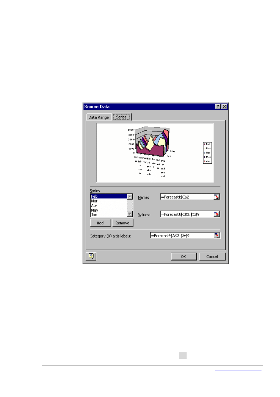
Excel 2002 Advanced Level
Charts
Page
129
To change series properties:
Mouse
1.
Choose Chart from the menu bar, then Source Data. The following
dialog box will appear:
2.
Ensure the Series tab is selected. Select the series whose
properties you want to change.
3.
Use the Name text box either to select a cell containing or type a
new name for the series.
4.
Use the Values text box to select the cells on the worksheet that
contain the values to be plotted on the chart for the selected series.
5.
Use the Category X-Axis labels text box to select the cells on the
worksheet containing the items you want as labels on the category
axis.
6.
When all options have been set, click OK.
© MTC Training Solutions Ltd

Excel 2002 Advanced Level
Charts
Page
130
© MTC Training Solutions Ltd
Charting with Blocks of Data
As it is possible to select separate ranges in Excel, it is possible to produce charts based
on non-contiguous data. This is vital if some of the information on the worksheet is to be
omitted. There are some guidelines to be aware of however. The layout of data is
important as was demonstrated at the beginning of this document. The selected ranges
must amount to a regular block with consistent height and width measurements so that
Excel can interpret it correctly, with categories and data series matching up.
Once the data has been successfully selected, choose File, New and click on Chart before
clicking on OK, or tap [F11].
An extension of this idea leads to the fact that ranges from separate worksheet files can be
included in a single chart. Simply select the worksheet data to be included (subject to the
layout provisos above), copy to the clipboard then paste them into the chart.
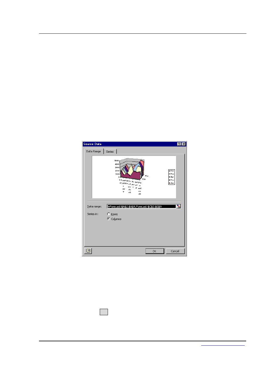
Excel 2002 Advanced Level
Charts
Page
131
Swapping the x and y axes
It has been seen that Excel will assign either rows or columns of data to be categories (as
opposed to data series) on the assumption that there will be more categories than data
series in the chart. Frequently this will produce satisfactory results, but there may be
times when you wishes to override Excel's decision.
To swap the x and y axes:
Mouse
1.
Select the chart.
2.
Choose Chart from the menu bar, then Source data.
3.
Ensure the Data Series tab is selected.
4.
Click the Rows or Columns option button (depending on what
the current orientation is) to change the order in which the items
are plotted.
5.
Click OK to confirm your changes.
© MTC Training Solutions Ltd

Excel 2002 Advanced Level
Charts
Page
132
© MTC Training Solutions Ltd
Using Charts to change Data
Another interesting aspect to Excel Charts hinges on the fact that a chart is linked to its
source data. You will probably have observed that changing a figure in a supporting
spreadsheet will affect a dependent chart. The marker representing that figure will adjust
to reflect the new value.
On a 2-dimensional chart this can be turned around to allow you to adjust a marker and
have the worksheet figure update automatically.
To change the value of a data marker:
Mouse
1.
Hold down [CTRL] and click on the data marker (bar, column etc.)
to be adjusted.
2.
A black selection handle will appear on the marker. Drag this to a
new position, and while doing so, a moving tick mark on the y-axis
indicates the current value. This will also be reflected in the
reference area.
3.
Release the marker at the new position and the relevant figure in
the worksheet will update.
The above procedure only works if the data marker represents a simple
number. If the marker represents a dependent formula, the Goal Seek
dialogue box will appear. You will then be asked which cell can be
changed in order to bring the dependent formula up or down to the value
to which you have dragged it.
This option will not work with 3-D charts.

Excel 2002 Advanced Level
Charts
Page
133
© MTC Training Solutions Ltd
Picture Charts
It is possible to substitute pictures or symbols representing data for the usual Excel chart
markers. You may use ready-made bitmap files, or may choose to draw his or her own
pictures for use in the chart. Any picture which can be copied to the clipboard may be
used for Picture Charts.
Create a Picture Chart
In order to create a Picture Chart, you should start by preparing a 2-D column, bar or line
chart in the usual way.
To replace data markers with pictures:
Mouse
1.
Select the data series whose markers you want to replace with
pictures.
2.
Choose Insert from the menu bar, then Picture, From File.
3.
Excel will offer you a file open dialog. Point Excel to the ClipArt
folder.
The position of this folder may vary depending on the installation of Office
’2003. It is generally a subfolder of the Microsoft Office folder.
4.
Select the picture you want to use and click OK. The picture will
appear in place of the previous data marker.

Excel 2002 Advanced Level
Charts
Page
134
If the picture is being pasted into a column or bar chart, it tends to stretch out to the same
size as the column or bar which it is replacing. This frequently results in distortion. You
may adjust this as necessary and the process for doing so is described over the
page.Formatting the Picture Chart
To format the picture settings:
Mouse
1.
Select one of the pictures by clicking on it.
2.
Choose Format from the menu bar, then Selected data series.
3.
From the resulting dialog box, ensure that the Patterns tab is
selected and click Fill Effects.
© MTC Training Solutions Ltd

Excel 2002 Advanced Level
Charts
Page
135
4.
Ensure the Picture tab is selected.
5.
Use the Format options to adjust whether the picture stretches to
the value of the plot point, (Stretch) or whether you want to stack
miniaturised pictures 1 to 10 units (Stack and Scale).
6.
When the desired effect has been achieved, click OK.
If the Stretch option button is selected, this indicates that the picture is sizing itself to
reflect the appropriate data. You may choose the Stack option to have the picture appear
in it's original size and stack copies to represent the value for each data point. Stack and
Scale will allow you to define precisely how much data is represented by each stacked
picture.
Remove Pictures from Chart
In order to revert to the normal chart markers, simply select the data series with pictures
and format the patterns back to a colour.
© MTC Training Solutions Ltd

Excel 2002 Advanced Level
Charts
Page
136
© MTC Training Solutions Ltd
☺
Useful Information
You can copy and paste any chart created in Excel into a Word document or a PowerPoint
slide.

Excel 2002 Advanced Level
Charts
Page
137
© MTC Training Solutions Ltd
.
Notes

Excel 2002 Advanced Level
Charts
Page
138
© MTC Training Solutions Ltd

Excel 2002 Advanced Level
Templates
Page
139
© MTC Training Solutions Ltd
Section 5
Templates
Objectives
By the end of this section you will be able to:
Use the standard Excel templates
Create Custom templates
Open and edit templates
Set template properties

Excel 2002 Advanced Level
Templates
Page
140
© MTC Training Solutions Ltd
Introduction to templates
A template is a file used as a form to create other workbooks, sheets and charts. New
workbooks created from the template contain the same layout, data, formulae, formats
and styles as those of the template. New sheets and charts inserted into a workbook are a
copy of the sheet or chart template.
Standard templates
Excel comes supplied with a selection of templates designed to help in the production of
common business and home financial tasks. These templates can be modified for
personal use.
To use a standard template:
Mouse
1.
Choose File from the menu bar, then New. Then select from the
general templates hyper-link on the task bar.
2.
Click the Spreadsheet Solutions tab to see a list of Excel
templates.
3.
Double-click on the icon for the template you wish to base the new
workbook on.
Custom templates
You can create your own workbook and sheet templates.
To create a workbook template:
Mouse
1.
Open or create the workbook to be used as the basis for the
template.
2.
Choose File from the menu bar, then Save As.
3.
Type the template name in the File name text box.

Excel 2002 Advanced Level
Templates
Page
141
© MTC Training Solutions Ltd
4.
Select Template from the Save as Type list. An .XLT extension
will be added to the template name.
5.
The folder where the file will be stored will automatically change
to Templates. By storing all .XLT files in the same folder Excel
recognises and keeps track of templates.
6.
Click OK to save the template.
To create a worksheet template:
Mouse
1.
In a new or existing workbook delete all the sheets except the one
to be used as the template.
2.
Choose File from the menu bar, then Save As.
3.
Type the template name in the File Name box.
4.
Select Template from the Save as Type list. An .XLT extension
will be added to the template name.
5.
The folder where the file will be stored will automatically change
to Templates. By storing all .XLT files in the same folder Excel
recognises and keeps track of templates.
6.
Click OK to save the template.
To base a new workbook on a template:
Mouse
1.
Choose File from the menu bar, then New
2.
The dialog box containing Excel’s own templates should now list
any custom templates that you have created.
3.
Click the icon for the template that you want to base the new
workbook on.
To add a worksheet based on a sheet template:
Mouse
1.
Click the right mouse button over a sheet tab and choose Insert.

Excel 2002 Advanced Level
Templates
Page
142
© MTC Training Solutions Ltd
2.
Double-click the icon for the worksheet template you want to base
the new sheet on.
Autotemplates
An autotemplate is a workbook saved as a template in the XLSTART folder or alternate
startup folder using the specific filename Book.xlt, sheet.xlt, dialog.xlt or macro.xlt.
Autotemplates if they exist will act as the basis for all new items you create in the Excel
environment.
The Book.xlt template becomes the default workbook. The Sheet.xlt template becomes
the default worksheet.
Opening and editing templates
Templates are files just like workbooks. If you need to change a template in any way,
simply open, edit and save in the normal way.
To open a template:
Mouse
1.
Choose File from the menu bar, then Open.
2.
Change the Look In location to the Templates folder.
3.
Double-click the name of the template you want to open.
To edit a template:
Mouse
1.
Make changes in the open template.
2.
Choose File from the menu bar, then Save.
Template properties
Files have various properties that are saved with them. Some properties, such as date
created and last saved date are included and updated automatically by Excel. Others,

Excel 2002 Advanced Level
Templates
Page
143
© MTC Training Solutions Ltd
such as title and subject must be entered manually by the user. Properties are helpful
when trying to locate files as you can use the properties to search.
To set template properties:
Mouse
1.
With the template open click File, Properties.
2.
Set the properties that apply to the template.
3.
Click OK.

Excel 2002 Advanced Level
Templates
Page
144
© MTC Training Solutions Ltd
☺
Useful Information
Templates can contain custom number formats and predefined styles.

Excel 2002 Advanced Level
Templates
Page
145
© MTC Training Solutions Ltd
.
Notes

Excel 2002 Advanced Level
Templates
Page
146
© MTC Training Solutions Ltd

Excel 2002 Advanced Level
Auditing
Page
147
© MTC Training Solutions Ltd
Section 6
Auditing
Objectives
By the end of this section you will be able to:
Use and understand tracers
Insert and use cell comments
Use validation circles
Use go to special

Excel 2002 Advanced Level
Auditing
Page
148
© MTC Training Solutions Ltd
Auditing features
Tracers
The precedent, dependent and error tracers display arrows on the worksheet to represent
the flow of computations:
Tracer Type
Arrow type
Formula Solid
blue
Error Solid
red
External reference or reference
to other worksheet
Dashed black with an icon
Comments
Comments are text or audio messages attached to cells usually giving a more detailed
explanation of a cells contents.
Validation circles
Validation circles are used to identify all cells that contain values that are outside the
limits set by using the Data, Validation menu option.
Go to Special
A method of selecting cells with particular contents or properties.

Excel 2002 Advanced Level
Auditing
Page
149
Precendents and Dependants
Precedents are cells referred to by other formulae. Dependants are cells containing
formulae that refer to other cells.
A direct precedent is a cell referred to by the formula in the active cell. An indirect
precedent is a cell referred to by a formula in a direct precedent cell or another indirect
precedent cell.
A direct dependant is a cell containing a formula that refers to the active cell. An indirect
dependent is a cell that contains a formula that refers to a direct dependant cell or another
indirect dependant cell.
You use the Auditing toolbar to set auditing options.
To view the Formula Auditing toolbar:
Mouse
1.
Choose Tools from the menu bar, then Auditing, Show Auditing
toolbar.
To audit for direct and indirect precedents:
Mouse
1.
Click on the cell you want to audit.
2.
Click the trace precedents button on the Auditing toolbar.
To audit for direct and indirect dependants:
Mouse
1.
Click on the cell you want to audit.
2.
Click the trace dependants button on the Auditing toolbar.
Click either button a second time to view indirect precedents or
dependants of the active cell.
© MTC Training Solutions Ltd

Excel 2002 Advanced Level
Auditing
Page
150
To remove the tracer arrows:
Mouse
1.
Click the remove precedent arrows to remove precedent tracers or
remove dependant arrows to remove dependant tracers.
Or
Click the remove all arrows button to remove both precedent and
dependant tracers.
© MTC Training Solutions Ltd

Excel 2002 Advanced Level
Auditing
Page
151
© MTC Training Solutions Ltd
Comments
When a cell has a comment attached, Celltips automatically display the comments added
when the mouse pointer rests over the cell. You can tell which cells have comments
attached as they have a comment indicator (a small red corner triangle).
To add a comment:
Mouse
1.
Click in the cell where you want to insert a comment.
2.
Choose Comment from the Insert menu.
3.
In the text box, type your comment.
4.
Click outside the text box to confirm the entry.
To view comments:
Mouse
1.
Position your mouse over the top of the cell that contains the
comment.
2.
Your comment will be displayed as a celltip.
To format comments:
Mouse
1.
Click the right-mouse button over the cell containing the comment
to format.
2.
Choose Show comment from the shortcut menu
3.
Choose Format from the menu bar, then comment to change the
font or the colour of the comment.

Excel 2002 Advanced Level
Auditing
Page
152
To edit comments:
Mouse
1.
Click on the cell that contains the comment you want to edit.
2.
Choose Edit Comment from the Insert menu.
3.
Click outside the comment box when you have finished.
Hiding and redisplaying comments:
Mouse
1.
You can hide an individual comment by clicking the right mouse
button over the cell that contains the comment and choosing Hide
comment from the shortcut menu.
2.
When you want to redisplay all individually hidden comments.
Choose View from the menu bar, then Comments and repeat.
To print comments:
Mouse
1.
On the File menu, choose Page Setup and click the Sheet tab.
2.
In the Comments box, choose At end of sheet
Or
Choose As displayed on sheet
3.
Click OK.
Reviewing comments:
Mouse
1.
Choose Comments on the View menu
2.
To view each comment in sequence click the Next Comment
button on the Reviewing toolbar.
© MTC Training Solutions Ltd

Excel 2002 Advanced Level
Auditing
Page
153
3.
To view the comments in reverse order, click the Previous
Comment button on the Reviewing toolbar.
© MTC Training Solutions Ltd

Excel 2002 Advanced Level
Auditing
Page
154
© MTC Training Solutions Ltd
☺
Useful Information
Auditing options can also be set using the Tools menu.

Excel 2002 Advanced Level
Auditing
Page
155
© MTC Training Solutions Ltd
.
Notes
Document Outline
- How to use this guide
- Names
- Conditional & Logical Functions
- Lookup Functions
- Goal Seeking and Solving
- SOLVER
- Views & Scenarios
- Excel Lists
- Sorting Data
- Adding subtotals to a list
- Filtering a List
- Data Form
- Advanced Filtering
- Copying filtered data
- List Statistics
- Pivot Tables
- Introduction to Charting
- ChartWizard
- Chart Types
- Manipulating Chart Data
- Picture Charts
- Introduction to templates
- Auditing features
- Precendents and Dependants
- Comments
Wyszukiwarka
Podobne podstrony:
Excel 2003 PL cwiczenia zaawansowane czex23
Excel 2003 PL Kurs
Microsoft Excel 2010 PL Jezyk VBA i makra Akademia Excela e21vba
Microsoft Excel dla Windows
Excel 2003 Programowanie Zapiski programisty
Excel 2003 PL cwiczenia praktyczne Wydanie II cwexc2
Excel 2003 PL Programowanie w VBA Vademecum profesjonalisty
excel 2003 pl kurs rozdział helion QLZRQABS235RF6JST6R6LU5DEUUVBRVWUZJX3SI
Excel 2003 PL cwiczenia praktyczne cwex23
Nowy Arkusz programu Microsoft Excel
EXCEL 2003 Kurs VBA
Pisanie makropoleceń w MS Excel 2003, Opisy programów FREE
Excel 2003 2007 Tworzenie makr w VBA Ćwiczenia zaawansowane
więcej podobnych podstron
