arXiv:1010.5885v1 [cond-mat.soft] 28 Oct 2010

Critical Scaling of Shearing Rheology at the Jamming Transition of Soft Core

Frictionless Disks

Peter Olsson

1

and S. Teitel

2

1

Department of Physics, Ume˚

a University, 901 87 Ume˚

a, Sweden

2

Department of Physics and Astronomy, University of Rochester, Rochester, NY 14627

(Dated: October 29, 2010)

We perform numerical simulations to determine the shear stress and pressure of steady-state

shear flow in a soft-disk model in two dimensions at zero temperature in the vicinity of the jamming
transition φ

J

. We use critical point scaling analyses to determine the critical behavior at jamming,

and we find that it is crucial to include corrections to scaling for a reliable analysis. We find that the
relative size of these corrections are much smaller for pressure than for shear stress. We furthermore
find a superlinear behavior for pressure and shear stress above φ

J

, both from the scaling analysis

and from a direct analysis of pressure data extrapolated to the limit of vanishing shear rate.

PACS numbers: 45.70.-n, 64.60.-i

Granular materials, supercooled liquids, and foams are

examples of systems that may undergo a transition from
a liquid-like to an amorphous solid state as some control
parameter is varied. It has been hypothesised that the
transitions in these strikingly different systems are con-
trolled by the same mechanism [1] and the term jamming
has been coined for this transition.

Much work on jamming has focused on a particularly

simple model, consisting of frictionless spherical particles
with repulsive contact interactions at zero temperature
[2]. The packing fraction (density) of particles φ is the
key control parameter in such systems. Jamming upon
compression, and jamming by relaxation from initially
random states, have been the focus of many investiga-
tions [2, 9, 11]. Another, physically realizable and impor-
tant case is jamming upon shear deformation. This has
been modeled both by simulations at a finite constant
shear strain rate ˙γ [3–8, 10], as well as by quasistatic
shearing [11, 15, 17], in which the system relaxes to its
energy minimum after each finite small strain increment.

Several attempts have been made to determine the crit-

ical packing fraction φ

J

and critical exponents, describing

behavior at shear driven jamming [3–8]. There is how-
ever little agreement on the values of the exponents and
there is thus a need for a thorough and careful investi-
gation of the jamming transition in the shearing ensem-
ble. It will also be interesting to compare the exponents
found from shearing rheology to those found from com-
pressing marginally jammed packings. In particular we
note the linear increase of pressure above jamming that
is observed in that system [2, 9], compared to the super-
linear behavior often reported in the sheared system for
pressure and/or shear stress [3, 4, 7, 8].

In this Letter we do a careful scaling analysis of high

precision data for both shear stress and pressure at shear
strain rates down to ˙γ = 10

−8

. Instead of relying on

visually acceptable data collapses we use a non-linear
minimization technique to determine the best fitting pa-
rameters. As in a recent analysis of energy-minimized

configurations [11] we find that it is necessary to include
corrections to scaling

, but also that the magnitude of the

corrections are markedly different for different quantities,
and, furthermore, that the neglect of these corrections is
a major reason for the differing values for the critical ex-
ponents in the literature. We find strong evidence for a
superlinear behavior of yield stress and pressure above
jamming from the scaling analysis, and also find inde-
pendent support for this result from pressure data ex-
trapolated to the limit of vanishing shear rate. We also
suggest a possible mechanism behind this behavior.

Following O’Hern et al. [2] we use a simple model of

bi-disperse frictionless soft disks in two dimensions with
equal numbers of disks with two different radii in the
ratio 1.4. Length is measured in units of the diameter
of the small particles, d

s

.

With r

ij

the distance be-

tween the centers of two particles and d

ij

the sum of

their radii, the interaction between overlapping particles
is V (r

ij

) = (ǫ/2)(1 − r

ij

/d

ij

)

2

. We use Lees-Edwards

boundary conditions [12] to introduce a time-dependent
shear strain γ = t ˙γ. With periodic boundary conditions
on the coordinates x

i

and y

i

in an L × L system, the

position of particle i in a box with strain γ is defined as

r

i

= (x

i

+ γy

i

, y

i

). We simulate overdamped dynamics

at zero temperature with the equation of motion [13],

dr

i

dt

= −C

X

j

dV (r

ij

)

dr

i

+ y

i

˙γ ˆ

x,

with ǫ = 1 and C = 1. The unit of time is τ

0

= d

s

/Cǫ.

All our simulations at the lower shear rates are from N ≥
65536 total particles.

Our basic scaling assumption describes how different

quantities, as e.g. shear stress, pressure, potential energy
and jamming fraction, depend on a change of length scale
with a scale factor b:

O(δφ, ˙γ, 1/L) = b

−

y

O

/ν

g

O

(δφb

1

/ν

, ˙γb

z

, b/L).

(1)

Here δφ = φ − φ

J

, y

O

is the critical exponent of the

observable O, ν is the correlation length exponent, and

2

10

−8

10

−7

10

−6

10

−5

10

−4

0.03

0.04

0.05

0.06

0.07

0.08

0.09

0.1

0.8416

0.8424

0.8428

0.8433

0.8436

0.8440

0.8444

˙γ

p/

˙γ

0.

3

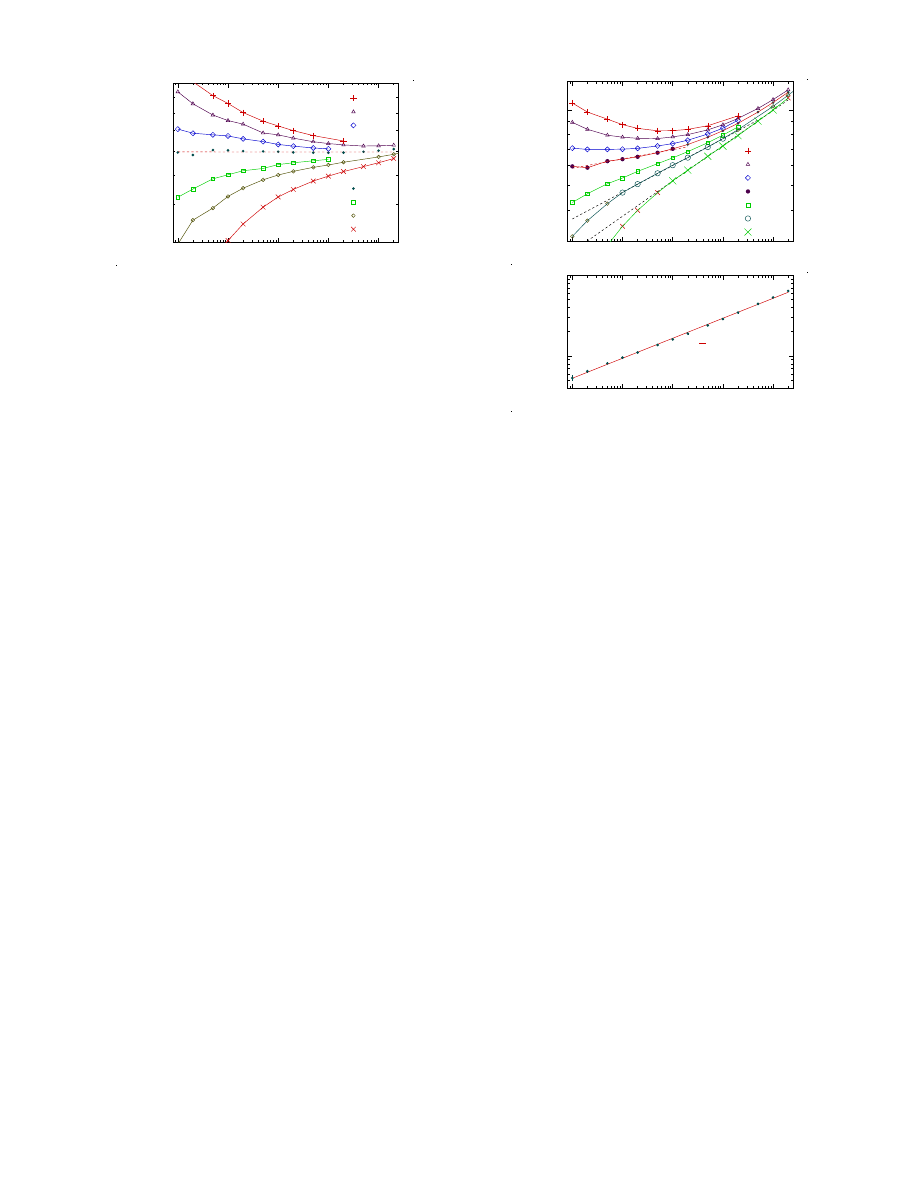
FIG. 1. Approximate determination of φ

J

and q

p

from Eq. (2)

without corrections to scaling. The figure shows pressure ver-
sus shear rate at several different packing fractions. The pres-
sure is shown as p/ ˙γ

0

.3

to make the behavior clearly visible.

This suggests that p ∼ ˙γ

q

1

with q

1

= 0.30 at φ

J 1

= 0.8433.

z is the dynamic critical exponent. Point J is at δφ = 0,

˙γ → 0, and an infinite system size, 1/L → 0; the scaling

relation describes the departure from the critical point in
these respective directions.

The above expression may be used as a starting point

for our analysis. We make use of data obtained at finite
shear rates and system sizes large enough that finite size
effects may be neglected — essentially the same approach
as in Ref. [3]. With b = ˙γ

−1

/z

in Eq. (1) and q

O

≡ y

O

/zν,

the scaling relation becomes

O(δφ, ˙γ) ∼ ˙γ

q

O

g

O

(δφ/ ˙γ

1

/zν

),

(2)

where the scaling function is a function of only a single
argument. At φ

J

we have O(φ

J

, ˙γ) ∼ ˙γ

q

O

which gives

a simple method for determining q

O

and φ

J

: Plot O

versus ˙γ on a double-log scale for several different φ. The
packing fraction for which the data fall on a straight line
is then our estimated φ

J

. Data above and below φ

J

,

respectively, should curve in opposite directions.

We start by applying this simple recipe to the pressure,

p, and will turn to the shear stress only as the next step.
Both these quantities are calculated, as in Ref. [2], from
the elastic forces only. Figure 1 shows pressure versus
shear rate at several different packing fractions. Antic-
ipating that the value of q

p

≈ 0.3, we plot p/ ˙γ

0

.3

vs ˙γ

in order to more clearly differentiate the behaviors near
φ

J

. It is then easy to identify the density with a recti-

linear behavior, and we find p ∼ ˙γ

q

1

with q

1

= 0.3 at

φ

J1

= 0.8433. Data at lower and higher densities curve

downwards and upwards, respectively. These values φ

J1

and q

1

are only first estimates of the jamming density

and the exponent, respectively; our final estimates turn
out to be just slightly different.

Figure 2 is the same kind of plot for the shear stress,

σ, and it is immediately clear that these data are not
directly amenable to the same kind of analysis; there is no
density with an algebraic behavor across the whole range
of shear rates. Before presenting our further analyses we

10

−8

10

−7

10

−6

10

−5

10

−4

0.003

0.004

0.005

0.006

0.007

0.008

0.009

0.01

0.8428

0.8436

0.8440

0.8444

(a)

0.8416

0.8424

0.8433

˙γ

σ

/

˙γ

0.

3

10

−8

10

−7

10

−6

10

−5

10

−4

10

−3

10

−2

h

0

˙γ

˜

ω

0

˜

ω

0

= 0.25

φ

J1

= 0.8433

q

1

= 0.30

g

1

= 0.0054

(b)

˙γ

σ

/

˙γ

q

1

−

g

1

FIG. 2. Shear stress σ versus shear rate ˙γ at several different
densities. Panel (a) shows that there is no density where σ
behaves algebraically across the extended range of shear rates,
however data across two orders of magnitude of ˙γ could, to
a reasonable approximation, be taken as algebraic. In that
vein, data limited to 10

−6

≤ ˙γ gives φ = 0.8416 (crosses) as a

good candidate for φ

J

(cf. Ref. [3]) whereas other ranges of ˙γ

would give other estimates. From a comparison with p/ ˙γ

q

1

=

const at φ

J 1

in Fig. 1, panel (b) shows the correction term

σ/ ˙γ

q

1

− g

1

at φ

J 1

, and it appears that this correction to a

very good approximation is ∼ ˙γ

˜

ω

0

, which has the same form

as standard corrections to scaling in critical phenomena.

note that this provides an explanation for the differing
values of both jamming density and exponents in the
literature. In Ref. [3] the jamming density was found to
be ≈ 0.8415 and the figure shows that data in the range
10

−6

≤ ˙γ ≤ 10

−4

would suggest φ = 0.8416 (crosses) as

a good candidate for φ

J

. However, it is clear that data

at the same density and lower shear rates deviate from
the algebraic behavior. Similarly, with access to σ down
to ˙γ = 10

−7

, φ = 0.8424 (open circles) would appear as a

good candidate for φ

J

, whereas data in the range 10

−8

≤

˙γ ≤ 10

−6

would suggest φ

J

= 0.8433 (solid dots). The

value of the effective exponent q

σ

also changes: for these

three different ranges of shear rates we find q

σ

= 0.44,

0.41, and 0.33, respectively. Note that this explanation
is at variance with Ref. [8] where the differing exponents
are attributed to using data from a too large range in φ.
That explanation is not applicable here since our analyses
only consider data right at the presumed φ

J

.

As a step towards the final analysis we now consider

the shear stress at φ

J1

and focus on the deviation from

the algebraic behavior ∼ ˙γ

q

1

. From Fig. 2(a) we note

that σ/ ˙γ

q

1

in the limit of low ˙γ appears to saturate at a

finite value, 0.005 < g

1

< 0.006 and so we plot σ/ ˙γ

q

1

− g

1

in Fig. 2(b). It is then possible to adjust g

1

such that the

3

remainder is algebraic in ˙γ,

σ(φ

J,0

, ˙γ)/ ˙γ

q

1

= g

1

+ ˙γ

˜

ω

0

h

0

,

(3)

with the exponent ˜

ω

0

≈ 0.25.

The importance of this observation lies in the fact that

standard corrections to scaling modify Eq. (1) to give
precisely this form [14],

O(δφ, ˙γ)/b

y

O

/ν

= g

O

(δφb

1

/ν

, ˙γb

z

) + b

−

ω

h

O

(δφb

1

/ν

, ˙γb

z

),

where h

O

is another scaling function and ω is the correc-

tion to scaling exponent. Using b = ˙γ

−1

/z

in the above

then gives

O(δφ, ˙γ)/ ˙γ

q

O

= g

O

(δφ/ ˙γ

1

/zν

) + ˙γ

ω/z

h

O

(δφ/ ˙γ

1

/zν

). (4)

Equation (3) is just the special case when δφ = 0.

The above analysis of σ relied on φ

J1

and q

1

deter-

mined from the pressure data without corrections to scal-
ing. We now set out to analyze both pressure and shear
stress directly from the scaling relation, Eq. (4), that in-
cludes the correction term, and determine the φ

J

, q

O

,

1/zν, and ω/z that allow for the best fit to Eq. (4). Here
g

O

and h

O

are scaling functions which we approximate

with fifth-order polynomials in x ≡ δφ/ ˙γ

1

/zν

. The actual

fits are done by minimizing χ

2

/dof with a Levenberg-

Marquardt method. The number of points in the fits
range from about 100 to 250 depending on the range of
data used in the fits.

In this kind of involved analysis it is crucial to validate

the results and to that end we use several different crite-
ria: (i) The first is to check the quality of the fits: Are
the deviations of the data from the scaling function con-
sistent with the statistical uncertainties? We use χ

2

/dof,

which should be close to unity to get a quantitative mea-
sure. (ii) A good quality of the fit does however not by
itself guarantee that the results are reliable. The sec-
ond check is therefore whether the fitting parameters are
reasonably independent of the precise range of the data
included in the fit. We do this by systematically varying
both the range of shear rates and the range of densi-
ties; fixing X = (φ − 0.8434)/ ˙γ

0

.26

we use the criterion

|X| < X

max

with X

max

= 0.2, 0.3, and 0.4. This restric-

tion does not reflect the size of the critical region but
rather that the polynomial approximation of the scaling
function breaks down for too large X. (iii) A final check
is whether the critical parameters from analyses of dif-
ferent quantities (here p and σ) agree with one another.

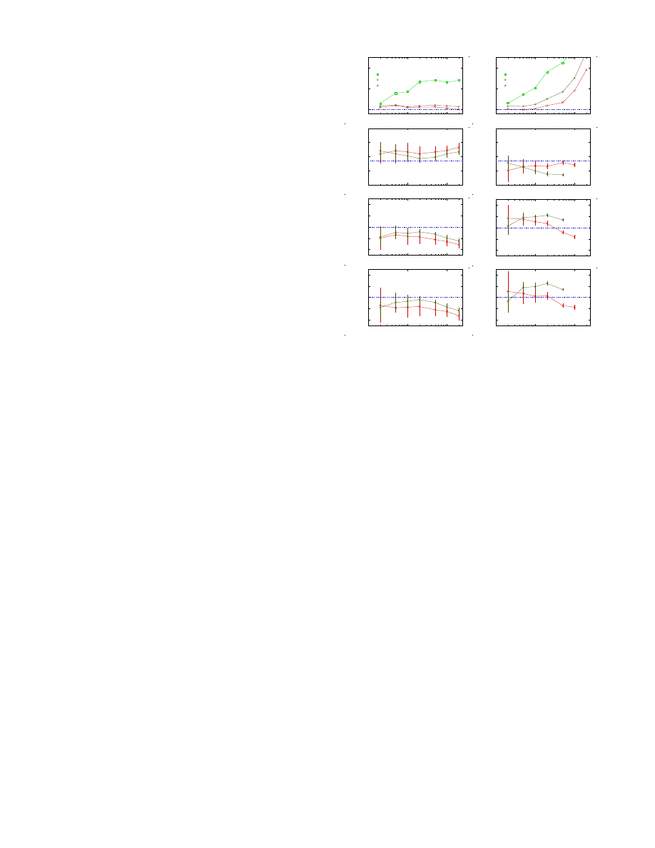
Figures 3 show χ

2

/dof and the key fitting parameters,

φ

J

, 1/zν, q

p

and q

σ

plotted against ˙γ

max

. For each quan-

tity the left and right panels are from analyses of pressure
and shear stress, respectively. First considering χ

2

/dof

in the first pair of panels, we note that the fits are only
good when the data are taken from a rather restrictive
interval in φ around φ

J

, |X| ≤ 0.3. For pressure there is a

good fit to the data over a very large interval—more than

10

−6

10

−5

10

−4

1

2

3

|X| ≤ 0.2

|X| ≤ 0.3

|X| ≤ 0.4

(a)

˙γ

max

χ

2

/d

of

10

−6

10

−5

10

−4

1

2

3

|X| ≤ 0.2

|X| ≤ 0.3

|X| ≤ 0.4

(b)

˙γ

max

χ

2

/d

of

10

−6

10

−5

10

−4

0.8433

0.8434

0.8435

0.8436

0.8437

(c)

˙γ

max

φ

J

10

−6

10

−5

10

−4

0.8433

0.8434

0.8435

0.8436

0.8437

(d)

˙γ

max

φ

J

10

−6

10

−5

10

−4

0.24

0.26

0.28

(e)

˙γ

max

1/

zν

10

−6

10

−5

10

−4

0.24

0.26

0.28

(f)

x

max

1/

zν

10

−6

10

−5

10

−4

0.26

0.28

0.30

(g)

˙γ

max

q

p

10

−6

10

−5

10

−4

0.26

0.28

0.30

(h)

˙γ

max

q

σ

FIG. 3. Results from scaling analyses that include corrections
to scaling. The left and right panels are from analyses of pres-
sure and shear stress, respectively. The first pair of panels,
which give χ

2

/dof, suggest that the analyses are only reliable

when data is used in a rather restrictive interval of φ − φ

J

,

|X| ≤ 0.3. For shear stress one also has to be restrictive in us-
ing data with larger ˙γ. From the following panels we read off
φ

J

= 0.84347, 1/zν = 0.26, and q

p

= q

σ

= 0.28. Combining

the last two (y = qzν) gives y

p

= y

σ

= 1.08.

four decades in ˙γ. For the shear stress the highest shear
rates should not be used, and reliable results are obtained
by restricting ˙γ to ˙γ ≤ 5 × 10

−5

when X

max

= 0.2 and

˙γ ≤ 1 × 10

−5

for X

max

= 0.3.

The next two panels show φ

J

from pressure and shear

stress, respectively, in good agreement with one an-
other; we estimate φ

J

= 0.84347 ± 0.00020 in agreement

with other recent determinations of φ

J

from quasistatic

simulations[11, 15]. Here and throughout, the error bars
in the figures are one standard deviation whereas the nu-
merical values give a min–max interval (± three standard
deviations) for the estimated quantities. To correctly in-
terpret these figures one should note that the fitted val-
ues for different ˙γ

max

and X

max

are based on different

subsets of the same data, and therefore are expected to
be strongly correlated. The main point is here to check
how robust the fitting parameters are to changes in the
precise data set, and the absence of clear trends in the
results is therefore an encouraging sign.

We further find 1/zν = 0.26 ± 0.02 and q = 0.28 ± 0.02.

Combining the two exponents we find y = qzν = 1.08 ±
0.03 (a strong correlation between q and 1/zν is re-
sponsible for the error estimate for y). Since y is just

4

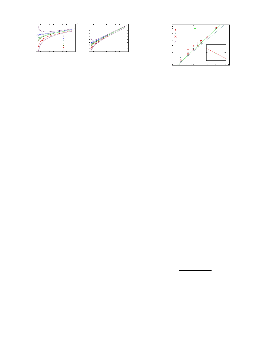
0.00

0.02

0.04

0.06

0.08

0.020

0.025

0.030

0.035

0.040

0.045

0.050

0.055

φ = 0.8424

φ = 0.8428

φ = 0.8432

φ = 0.8433

φ = 0.8434

φ = 0.8436

φ = 0.8440

˙γ

ω/z

p/

˙γ

q

p

0.00

0.02

0.04

0.06

0.08

0.002

0.004

0.006

0.008

0.010

˙γ

ω/z

σ

/

˙γ

q

σ

FIG. 4. Illustration of results of the scaling analysis. The
dashed lines are the behaviors at φ

J

for p and σ, respectively:

O(φ

J

, ˙γ)/ ˙γ

q

O

= g

O

(0) + ˙γ

ω/z

h

O

(0).

slightly above unity we have also reanalyzed the pres-
sure data with the assumption y

p

= 1. The fits then

become considerably worse and we conclude that the
data is strongly in favor of y

p

> 1. A similar analysis

of the shear stress is not conclusive. Using ν = 1.09
from Ref. [11] the dynamic critical exponent becomes
z = 3.5 ± 0.4. The correction to scaling exponent (not
shown) is ω/z = 0.29 ± 0.03, or ων = 1.10 ± 0.06, which,
again using ν = 1.09 [11], gives ω = 1.0 ± 0.1 in good
agreement with Ref. [11].

The analyses of both pressure and shear stress work

nicely when corrections to scaling are included. A draw-
back with including the corrections is—beside the more
difficult analyses—that it is no longer possible to deter-
mine φ

J

directly from a simple plot as in Fig. 1. The

most direct way to illustrate the determination of φ

J

is

shown in Fig. 4 which displays p/ ˙γ

q

p

and σ/ ˙γ

q

σ

against

˙γ

ω/z

, now with linear scales on both axes. Data at φ

J

should then fall on a straight line. Note the very different
size of the corrections, given by the slopes of the data.

For φ well above φ

J

the pressure decays algebraically in

˙γ and this gives a means to determine the limiting value

p(φ, ˙γ → 0). If we can get reliable values, p(φ, ˙γ → 0), at
densities sufficiently close above φ

J

it should be possible

to get another determination of y

p

, independent of the

scaling analysis. Fig. 5 shows some of our finite- ˙γ data
together with such extrapolated values for densities down
to φ = 0.848. Fitting to the five points from φ = 0.848
through 0.856 (0.5% through 1.5% above φ

J

) we find y =

1.09±0.04 shown by the solid line, in excellent agreement
with y = 1.08 from the scaling analysis. (The inset of
Fig. 5 shows how y depends on the assumed φ

J

.) Similar

results, y

p

≈ 1.1 have also been found before [16, 17].

The above results point to a good agreement between

the exponent obtained from the scaling analyses on the
one hand, and the ˙γ → 0 limit of the pressure above
φ

J

on the other. This is entirely in accordance with ex-

pectations from critical scaling. This is in contrast to
the claim in Ref. [8] that the critical region is extremely
narrow and doesn’t include densities away from φ

J

in the

limit ˙γ → 0; the yield stress is there taken to be governed
by a different regime with a different exponent, y

σ

= 3/2.

With the result y ≈ 1.1 from two different analy-

ses it becomes important to try and reconcile this with

0.005

0.01

0.05

10

−3

10

−2

˙γ = 10

−8

˙γ = 10

−7

˙γ = 10

−6

˙γ → 0

Slope = 1.09
Slope = 1

φ/φ

J

− 1

p(

φ

,

˙γ)

0.843

0.844

1.0

1.2

φ

J

y

FIG. 5. Alternative determination of the exponent y

p

. The

open circles are p(φ, ˙γ → 0) from extrapolations of p(φ, ˙γ).
Assuming φ

J

= 0.84347 the exponent becomes y = 1.09,

shown by the solid line. The dashed line corresponds to y = 1.
The inset shows how y depends on the assumed φ

J

.

the well established linear increase of the pressure when
marginally jammed packings are compressed above their
respective jamming densities [2, 9]. We speculate that the
reason for this is that the ensemble of configurations de-
pends in a non-trivial way on φ in the vicinity of φ

J

, and

that this is so since the dynamic process that generates
this ensemble

is itself very sensitive to φ. It is then rele-

vant to consider the behavior in the quasistatic limit and
to recall that the average time needed for the minimiza-
tion of energy in quasistatic simulations diverges as φ

J

is approached from above or from below. (This parallels
the more rapid jumping between jammed and unjammed
states reported in Ref. [15].) A dramatic change of the
dynamical process that generates the ensemble suggests
that the ensemble itself would depend on φ in a non-
trivial way.

To conclude, we have shown that pressure and shear

stress from shearing simulations are entirely consistent
with the assumption of a critical behavior when correc-
tions to scaling are included in the analysis. We find
φ

J

= 0.84347 ± 0.00020 and that at φ

J

, both p and σ

scale as ˙γ

q

with q = 0.28 ± 0.02. In the limit ˙γ → 0 both

p and σ vanish as (φ − φ

J

)

y

with y = 1.08 ± 0.03.

This work was supported by Department of En-

ergy Grant No. DE-FG02-06ER46298, Swedish Research
Council Grant No. 2007-5234, and a grant from the
Swedish National Infrastructure for Computing (SNIC)
for computations at HPC2N.

[1] A. J. Liu and S. R. Nagel, Nature (London) 396, 21

(1998).

[2] C. S. O’Hern, L. E. Silbert, A. J. Liu, and S. R. Nagel,

Phys. Rev. E 68, 011306 (2003).

[3] P. Olsson and S. Teitel, Phys. Rev. Lett. 99, 178001

(2007).

[4] T. Hatano, J. Phys. Soc. Jpn. 77, 123002 (2008).
[5] T. Hatano(2008), arXiv:0804.0477.
[6] M. Otsuki and H. Hayakawa, Phys. Rev. E 80, 011308

5

(2009).

[7] T. Hatano, Progr. Theor. Phys. Suppl. 184, 143 (2010).
[8] B. P. Tighe, E. Woldhuis, J. J. C. Remmers, W. van Saar-

loos, and M. van Hecke, Phys. Rev. Lett. 105, 088303
(2010).

[9] P. Chaudhuri, L. Berthier, and S. Sastry, Phys. Rev. Lett.

104

, 165701 (2010).

[10] T. Hatano, Phys. Rev. E 79, 050301 (2009).
[11] D. V˚

agberg, D. Valdez-Balderas, M. Moore, P. Olsson,

and S. Teitel(2010), arXiv:1010.4752.

[12] D. J. Evans and G. P. Morriss, Statistical Mechanics of

Nonequilibrium Liquids

(Academic Press, London, 1990).

[13] D. J. Durian, Phys. Rev. Lett. 75, 4780 (1995).
[14] K. Binder, Z. Phys. 43, 119 (1981).
[15] C. Heussinger and J.-L. Barrat, Phys. Rev. Lett. 102,

218303 (2009).

[16] T. S. Majmudar, M. Sperl, S. Luding, and R. P.

Behringer, Phys. Rev. Lett. 98, 058001 (2007).

[17] C. Heussinger, P. Chaudhuri, and J.-L. Barrat, Soft Mat-

ter 6, 3050 (2010).