2 ASOR BULLETIN, Volume 22 Number 2, June 2003

Refereed

Comparing ANN Based Models with ARIMA for Prediction of

Forex Rates

Joarder Kamruzzaman

a

and Ruhul A Sarker

b

Abstract

In the dynamic global economy, the
accuracy in forecasting the foreign currency
exchange (Forex) rates or at least
predicting the trend correctly is of crucial
importance for any future investment. The
use of computational intelligence based
techniques for forecasting has been proved
extremely successful in recent times. In this
paper, we developed and investigated three
Artificial Neural Network (ANN) based
forecasting models using Standard
Backpropagation (SBP), Scaled Conjugate
Gradient (SCG) and Backpropagation with
Baysian Regularization (BPR) for Australian
Foreign Exchange to predict six different
currencies against Australian dollar. Five
moving average technical indicators are
used to build the models. These models
were evaluated using three performance
metrics, and a comparison was made with
the best known conventional forecasting
model ARIMA. All the ANN based models
outperform ARIMA model. It is found that
SCG based model performs best when
measured on the two most commonly used
metrics and shows competitive results when
compared with BPR based model on the
third indicator. Experimental results
demonstrate that ANN based model can
closely forecast the forex market.


Introduction

The foreign exchange market has
experienced unprecedented growth over
the last few decades. The exchange rates
play an important role in controlling
dynamics of the exchange market. As a
result, the appropriate prediction of
exchange rate is a crucial factor for the
success of many businesses and fund
managers. Although the market is well-
known for its unpredictability and volatility,
there exist a number of groups (like Banks,
Agency and other) for predicting exchange
rates using numerous techniques.

Exchange rates prediction is one of the
demanding applications of modern time
series forecasting. The rates are inherently
noisy, non-stationary and deterministically
chaotic [3, 22]. These characteristics
suggest that there is no complete
information that could be obtained from the
past behaviour of such markets to fully
capture the dependency between the future
rates and that of the past. One general
assumption is made in such cases is that
the historical data incorporate all those
behaviour. As a result, the historical data is
the major player (/input) in the prediction
process. However, it is not clear how good
is these predictions. The purpose of this
paper is to investigate and compare two
well-known prediction techniques, under
different parameter settings, for several
different exchange rates.

For more than two decades, Box and
Jenkins’ Auto-Regressive Integrated
Moving Average (ARIMA) technique [1] has
been widely used for time series
forecasting. Because of its popularity, the
ARIMA model has been used as a
benchmark to evaluate many new modelling
approaches [8]. However, ARIMA is a
general univariate model and it is
developed based on the assumption that
the time series being forecasted are linear
and stationary [2].

The Artificial Neural Networks, the well-
known function approximators in prediction
and system modelling, has recently shown
its great applicability in time-series analysis
and forecasting [20-23]. ANN assists
multivariate analysis. Multivariate models
can rely on greater information, where not
only the lagged time series being forecast,
but also other indicators (such as technical,
fundamental, inter-marker etc. for financial
market), are combined to act as predictors.

a

Gippsland School of Computing and IT,

Monash University, Churchill, VIC 3842

b

School of CS, UNSW@ADFA, Canberra, ACT

2600

ASOR BULLETIN, Volume 22 Number 2, June 2003 3

In addition, ANN is more effective in
describing the dynamics of non-stationary
time series due to its unique non-
parametric, non-assumable, noise-tolerant
and adaptive properties. ANNs are
universal function approximators that can
map any nonlinear function without a priori
assumptions about the data [2].

In several applications, Tang and Fishwich
[17], Jhee and Lee [10], Wang and Leu [18],
Hill et al. [7], and many other researchers
have shown that ANNs perform better than
ARIMA models, specifically, for more
irregular series and for multiple-period-
ahead forecasting. Kaastra and Boyd [11]
provided a general introduction of how a
neural network model should be developed
to model financial and economic time
series. Many useful, practical
considerations were presented in their
article. Zhang and Hu [23] analysed
backpropagation neural networks' ability to
forecast an exchange rate. Wang [19]
cautioned against the dangers of one-shot
analysis since the inherent nature of data
could vary. Klein and Rossin [12] proved
that the quality of the data also affects the
predictive accuracy of a model. More
recently, Yao et al. [20] evaluated the
capability of a backpropagation neural-
network model as an option price
forecasting tool. They also recognised the
fact that neural-network models are context
sensitive and when studies of this type are
conducted, it should be as comprehensive
as possible for different markets and
different neural-network models.

In this paper, we apply ARIMA and ANNs
for predicting currency exchange rates of
Australian Dollar with six other currencies
such as US Dollar (USD), Great British
Pound (GBP), Japanese Yen (JPY),
Singapore Dollar (SGD), New Zealand
Dollar (NZD) and Swiss Franc (CHF). A
total 500 weeks (closing rate of the week)
data are used to build the model and 65
weeks data to evaluate the models. Under
ANNs, three models using standard
backpropagation, scaled conjugate gradient
and Baysian regression were developed.
The outcomes of all these models were
compared with ARIMA based on three
different error indicators. The results show
that ANN models perform much better than
ARIMA models. Scaled conjugate gradient
and Baysian regression models show
competitive results and these models
forecasts more accurately than standard

Backpropagation which has been studied
considerably in other studies.

After introduction, ARIMA, ANN based
forecasting models and the performance
metrics are briefly introduced. In the
following two sections, data collection and
experimental results are presented. Finally
conclusions are drawn.


ARIMA: An Introduction

The Box-Jenkins method [1 & 2] of
forecasting is different from most
conventional optimization based methods.
This technique does not assume any
particular pattern in the historical data of the
series to be forecast. It uses an iterative
approach of identifying a possible useful
model from a general class of models. The
chosen model is then checked against the
historical data to see whether it accurately
describes the series. If the specified model
is not satisfactory, the process is repeated
by using another model designed to
improve on the original one. This process is
repeated until a satisfactory model is found.

A general class of Box-Jenkins models for a
stationary time series is the ARIMA or
autoregression moving-average, models.
This group of models includes the AR
model with only autoregressive terms, the
MA models with only moving average
terms, and the ARIMA models with both
autoregressive and moving-average terms.
The Bob-Jenkins methodology allows the
analyst to select the model that best fits the
data. The details of AR, MA and ARIMA
models can be found in Jarrett [6 & 9]


Artificial Neural Network: An
Introduction

In this section we first briefly present
artificial neural networks and then the
learning algorithms used in this study to
train the neural networks.

Artificial Neuron

In the quest to build an intelligent machine
in the hope of achieving human like
performance in the field of speech and
pattern recognition, natural language
processing, decision making in fuzzy
situation etc. we have but one naturally
occurring model: the human brain itself, a

4 ASOR BULLETIN, Volume 22 Number 2, June 2003

highly powerful computing device. It follows
that one natural idea is to simulate the
functioning of brain directly on a computer.
The general conjecture is that thinking
about computation in terms of brain
metaphor rather than conventional
computer will lead to insights into the nature
of intelligent behavior. This conjecture is
strongly supported by the very unique
structure of human brain.

Digital computers can perform complex
calculations extremely fast without errors
and are capable of storing vast amount of
information. Human being cannot approach
these capabilities. On the other hand
humans routinely perform tasks like
common sense reasoning, talking, walking,
and interpreting a visual scene etc. in real
time effortlessly. Human brain consists of
hundred billions of neurons, each neuron
being an independent biological information
processing unit. On average each neuron is
connected to ten thousands surrounding
neurons, all act in parallel to build a
massively parallel architecture. What we do
in about hundred computational steps,
computers cannot do in million steps. The
underlying reason is that, even though each
neuron is an extremely slow device
compared to the state-of-art digital
component, the massive parallelism gives
human brain the vast computational power
necessary to carry out complex tasks.
Human brain is also highly fault tolerant as
we continue to function perfectly though
neurons are constantly dying. We are also
better capable of dealing with fuzzy
situations by finding closest matches of new
problem to the old ones. Inexact matching
is something brain-style model seem to be
good at, because of the diffuse and fluid
way in which knowledge is represented. All
these serve a strong motivation for the idea
of building an intelligent machine modeled
after biological neuron, now known as
artificial neural networks.

Artificial neural network models are very
simplified versions of our understanding of
biological neuron, which is yet far from
complete. Each neuron’s input fibre called
dendrite receives excitatory signals through
thousands of surrounding neurons’ output
fibre called axon. When the total summation
of excitatory signals becomes sufficient it
causes the neuron to fire sending excitatory
signal to other neurons connected to it.
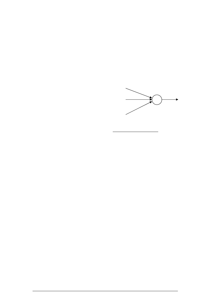
Figure 1 shows a basic artificial neural
network model. Each neuron receives an

input x

j

from other neuron j which is

multiplied by the connection strength called
weight

ω

j

(synaptic strength in biological

neuron) to produce total net input as the
weighted sum of all inputs as shown below.

x

j

j

j

net

∑

=

ω

The output of the neuron is produced by
passing the net input through an activation
function. The commonly used activation
functions are hard limiter, sigmoidal or
gaussian activation function.

Fig.1. An artificial neuron.

Neural Network Architecture

Neural networks can be very useful to
realize an input-output mapping when the
exact relationship between input-output is
unknown or very complex to be determined
mathematically. Because of its ability to
learn complex mapping, recently it has
been used for modelling nonlinear
economic relationship. By presenting a data
set of input-output pair iteratively, a neural
network can be trained to determine a set of
weights that can approximate the mapping.

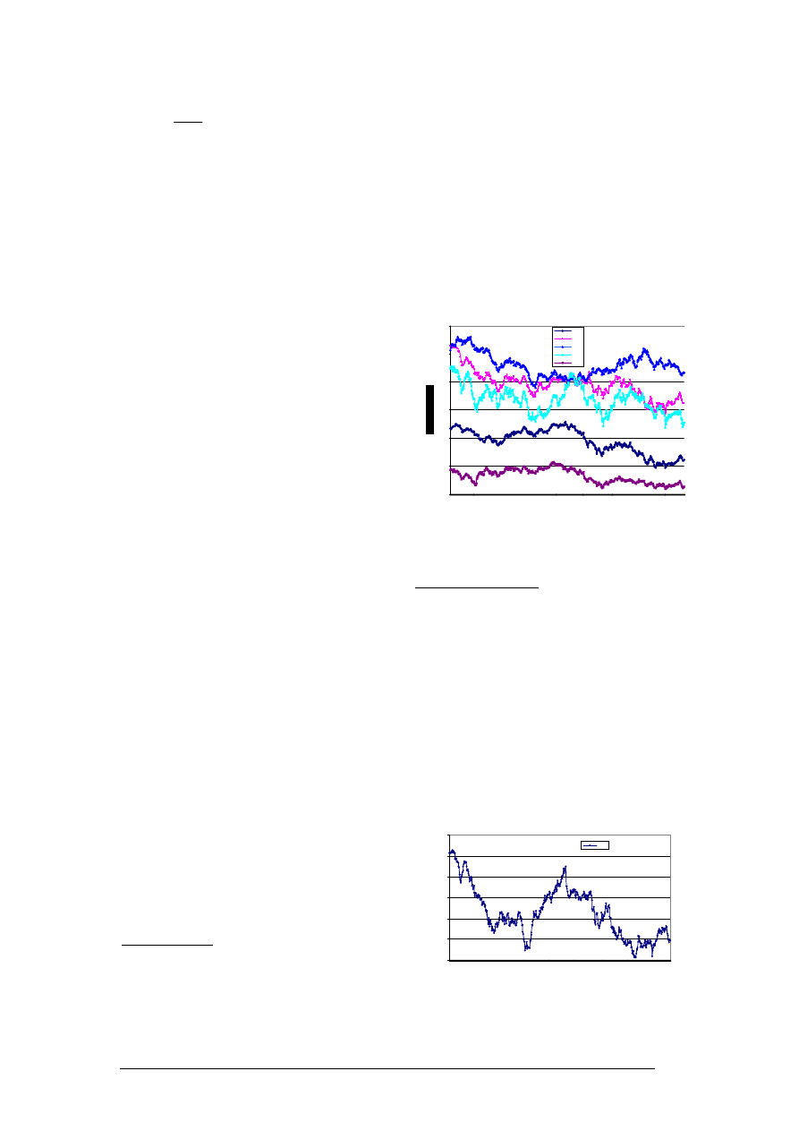
Multilayer feedforward network, as shown in
Fig. 2, is one of most commonly used
neural network architecture. It consists of
an input layer, an output layer and one or
more intermediate layer called hidden layer.
All the nodes at each layer are connected to
each node at the upper layer by
interconnection strength called weights. x

i

's

are the inputs,

ω

's are the weights, y

k

's are

output produced by the network. All the
interconnecting weights between layers are
initialized to small random values at the
beginning. During training inputs are
presented at the input layer and associated
target output is presented at the output
layer. A training algorithm is used to attain a
set of weights that minimizes the difference
the target output and actual output
produced by the network.

x

1

x

2

x

n

net

y=f(net)

output

ASOR BULLETIN, Volume 22 Number 2, June 2003 5

Fig. 2. A multiplayer feerforward ANN

structure.

There are many different neural net learning
algorithms found in the literature. No study
has been reported to analytically determine
the generalization performance of each
algorithm. In this study we experimented
with three different neural network learning
algorithms, namely standard
Backpropagation (BP), Scaled Conjugate
Gradient Algorithm (SCG) and
Backpropagation with regularization (BPR)
in order to evaluate which algorithm
predicts the exchange rate of Australian
dollar most accurately. In the following we
describe the three algorithms briefly.

Training Algorithms

Standard BP: BP [16] uses steepest
gradient descent technique to minimize the
sum-of-squared error E over all training
data. During training, each desired output d

j

is compared with actual output y

j

and E is

calculated as sum of squared error at the
output layer.

The weight

ω

j

is updated in the n-th training

cycle according to the following equation.

)

1

(

)

(

−

∆

+

∂

∂

−

=

∆

n

E

n

j

j

j

ω

α

ω

η

ω

The parameters

η

and

α

are the learning

rate and the momentum factor, respectively.
The learning rate parameter controls the
step size in each iteration. For a large-scale
problem Backpropagtion learns very slowly
and its convergence largely depends on
choosing suitable values of

η

and

α

by the

user.

SCGA: In conjugate gradient methods, a
search is performed along conjugate
directions, which produces generally faster
convergence than steepest descent
directions [5]. In steepest descent search, a

new direction is perpendicular to the old
direction. This approach to the minimum is
a zigzag path and one step can be mostly
undone by the next. In CG method, a new
search direction spoils as little as possible
the minimization achieved by the previous
one and the step size is adjusted in each
iteration. The general procedure to
determine the new search direction is to
combine the new steepest descent direction
with the previous search direction so that
the current and previous search directions
are conjugate as governed by the following
equations.

p

ω

ω

k

k

k

k

α

+

=

+1

,

p

ω

p

1

)

(

+

+

′

−

=

k

k

k

E

α

where p

k

is the weight vector in k-th

iteration, p

k

and p

k+1

are the conjugate

directions in successive iterations.

α

k

and

β

k

are calculated in each iteration. An
important drawback of CG algorithm is the
requirement of a line search in each
iteration which is computationally
expensive. Moller introduced the SCG to
avoid the time-consuming line search
procedure of conventional CG. SCG needs
to calculate Hessian matrix which is
approximated by

p

ω

p

ω

p

ω

k

k

k

k

k

k

k

k

k

E

E

E

λ

σ

σ

+

′

−

+

′

=

′′

)

(

)

(

)

(

where E' and E'' are the first and second
derivative of E. p

k

,

σ

k

and

λ

k

are the search

direction, parameter controlling the second
derivation approximation and parameter
regulating indefiniteness of the Hessian
matrix. Considering the machine precision,
the value of

σ

should be as small as

possible (

≤ 10

-4

). A detailed description of

the algorithm can be found in [15].

BPR: A desired neural network model
should produce small error on out of sample
data, not only on sample data alone. To
produce a network with better
generalization ability, MacKay [14]
proposed a method to constrain the size of
network parameters by regularization.
Regularization technique forces the network
to settle to a set of weights and biases
having smaller values. This causes the
network response to be smoother and less
likely to overfit [5] and capture noise. In
regularization technique, the cost function F
is defined as

j

y

k

i

x

i

ω

j
i

h

j

ji

ω

k
j

Output

Hidden layer

Input layer

6 ASOR BULLETIN, Volume 22 Number 2, June 2003

∑

=

−

+

=

n

j

j

n

E

F

1

2

1

ω

γ

γ

where E is the sum-squared error and

γ

(<1.0) is the performance ratio parameter,
the magnitude of which dictates the
emphasis of the training. A large

γ

will drive

the error E small whereas a small

γ

will

emphasize parameter size reduction at the
expense of error and yield smoother
network response. Optimum value of

γ

can

be determined using Bayesian
regularization in combination with
Levenberg-Marquardt algorithm [4]

Neural Network Forecasting Model

Technical and fundamental analyses are
the two major financial forecasting
methodologies. In recent times, technical
analysis has drawn particular academic
interest due to the increasing evidence that
markets are less efficient than was
originally thought [13]. Like many other
economic time series model, exchange rate
exhibits its own trend, cycle, season and
irregularity. In this study, we used time
delay moving average as technical data.
The advantage of moving average is its
tendency to smooth out some of the
irregularity that exits between market days
[21]. In our model, we used moving average
values of past weeks to feed to the neural
network to predict the following week’s rate.
The indicators are MA5, MA10, MA20,
MA60, MA120 and X

i

, namely, moving

average of one week, two weeks, one
month, one quarter, half year and last
week's closing rate, respectively. The
predicted value is X

i+1.

So the neural

network model has 6 inputs for six
indicators, one hidden layer and one output
unit to predict exchange rate. Historical data
are used to train the model. Once trained
the model is used for forecasting.

Experimental Results

In this section, we present the data
collection procedure and the results of
experiments.

Data Collection

The data used in this study is the foreign
exchange rate of six different currencies
against Australian dollar from January 1991
to July 2002 made available by the Reserve

Bank of Australia. We considered exchange
rate of US dollar, British Pound, Japanese
Yen, Singapore dollar, New Zealand dollar
and Swiss Franc. As outlined in an earlier
section, 565 weekly data was considered of
which first 500 weekly data was used in
training and the remaining 65 weekly data
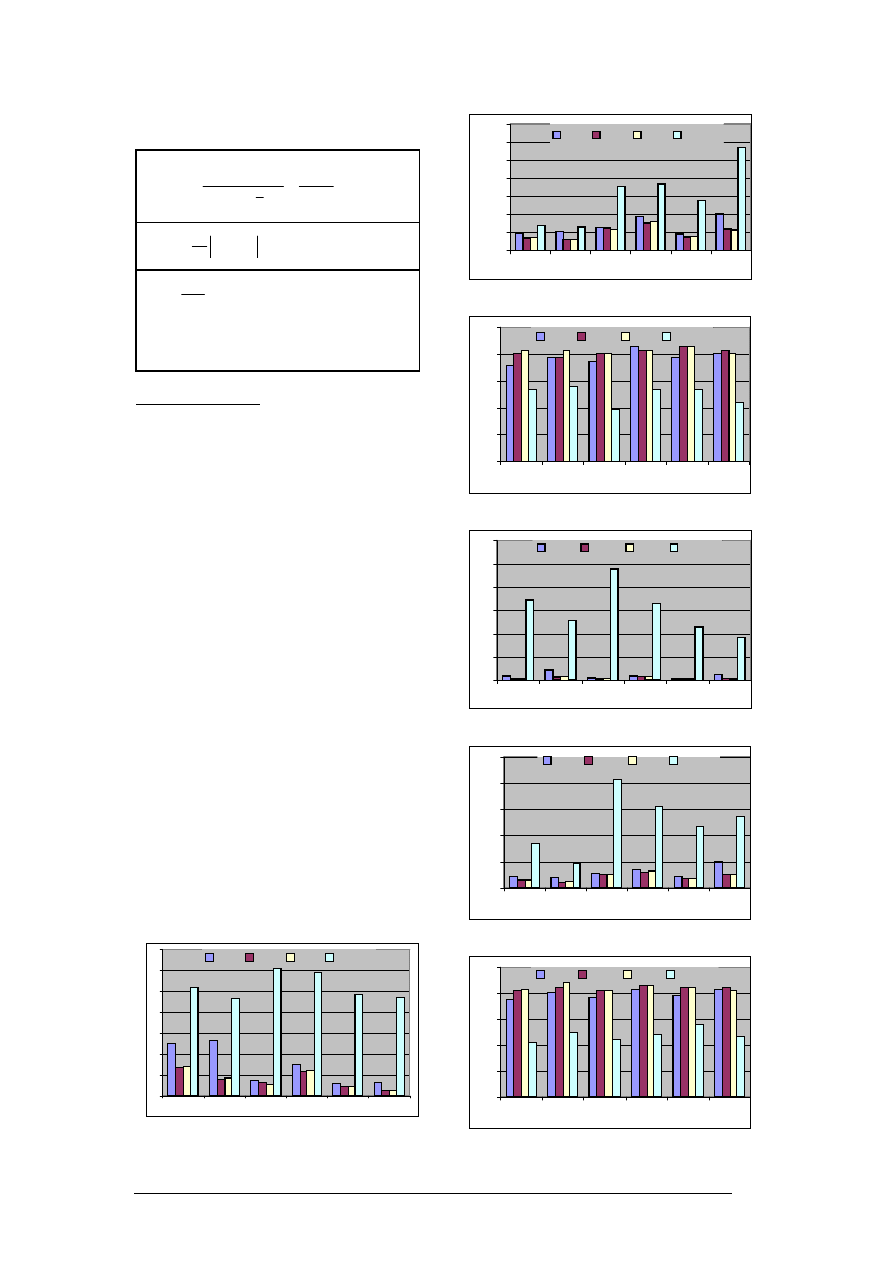
for evaluating the model. The plots of
historical rates for US Dollar (USD), Great
British Pound (GBP), Singapore Dollar
(SGD), New Zealand Dollar (NZD) and
Swiss Franc (CHF) are shown in Figure 3,
and for Japanese Yen (JPY) in Figure 4.

0.3

0.5

0.7

0.9

1.1

1.3

1.5

1

51

101

151

20

25

30

35

40

45

50

551

W eek N um b er

USD

SGD

NZD

CHF

GBP

Figure 3. Historical rates for USD, GBP,

SGD, NZD and CHF

Performance Metrics

The forecasting performance of the above
mentioned models is evaluated against
three widely used statistical metric, namely,
Normalized Mean Square Error (NMSE),
Mean Absolute Error (MAE) and Directional
Symmetry (DS). These criteria are defined
in Table 1. NMSE and MAE measure the
deviation between actual and forecasted
value. Smaller values of these metrics
indicate higher accuracy in forecasting. DS
measures correctness in predicted
directions and higher value indicates
correctness in trend prediction.

55

65

75

85

95

105

115

1

51

101

151

201

251

301

351

401

451

501

551

Week Number

Ex

ch

an

g

e R

at

e

JPY

Figure 4. Historical rates Japanese Yen

ASOR BULLETIN, Volume 22 Number 2, June 2003 7

Table 1: Performance metrics used in the

experiment.

∑

−

∑

−

∑

−

=

=

k

k

k

k

k

k

k

k

k

x

x

x

x

x

NMSE

N

x

)

(

)

(

)

(

ˆ

ˆ

2

2

2

2

1

σ

x

x

k

k

N

MAE

ˆ

1

−

=

∑

=

k

k

d

N

DS

100

,







≥

−

−

=

−

−

otherwise

0

)

ˆ

ˆ

(

)

(

if

0

1

1

1

x

x

x

x

k

k

k

k

k

d

Simulation Results

Simulation was performed with different
neural networks and ARIMA model. The
performance of a neural network depends
on a number of factors, e.g., initial weights
chosen, different learning parameters used
during training (described in section 2.3)
and the number of hidden units. For each
algorithm, we trained 30 different networks
with different initial weights and learning
parameters. The number of hidden units
was varied between 3~7 and the training
was terminated at iteration number between
5000 to 10000. The simulation was done in
MATLAB using modules for SBP, SCG and
BPR from neural network toolbox. The best
results obtained by each algorithm are
presented below. The ARIMA model (with
parameters setting 1,0,1) was run from
Minitab on a IBM PC.

After a model is built, exchange rate is
forecasted for each currency over the test
data. Prediction performance is measured
in terms of MNSE, MAE and DS over 35
weeks and 65 weeks by comparing the
forecasted and actual exchange rate.
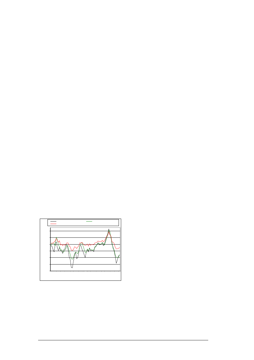
Figures 5(a)~(c) and 6(a)~(c) present the
performance metrics graphically over 35
and 65 weeks respectively.

0

0.2

0.4

0.6

0.8

1

1.2

1.4

USD

GBP

JPY

SGD

NZD

CHF

SBP

SCG

BPR

ARIMA

Fig. 5(a) NMSE over 35 weeks

0

0.005

0.01

0.015

0.02

0.025

0.03

0.035

USD

GBP

JPY

SGD

NZD

CHF

SBP

SCG

BPR

ARIMA

Fig. 5(b) MAE over 35 weeks

0

20

40

60

80

100

USD

GBP

JPY

SGD

NZD

CHF

SBP

SCG

BPR

ARIMA

Fig. 5(c) DS over 35 weeks

0

0.5

1

1.5

2

2.5

3

USD

GBP

JPY

SGD

NZD

CHF

SBP

SCG

BPR

ARIMA

Fig. 6(a) NMSE over 65 weeks

0

0.01

0.02

0.03

0.04

0.05

USD

GBP

JPY

SGD

NZD

CHF

SBP

SCG

BPR

ARIMA

Fig. 6(b) MAE over 65 weeks

0

20

40

60

80

100

USD

GBP

JPY

SGD

NZD

CHF

SBP

SCG

BPR

ARIMA

Fig. 6(c) DS over 65 weeks

8 ASOR BULLETIN, Volume 22 Number 2, June 2003

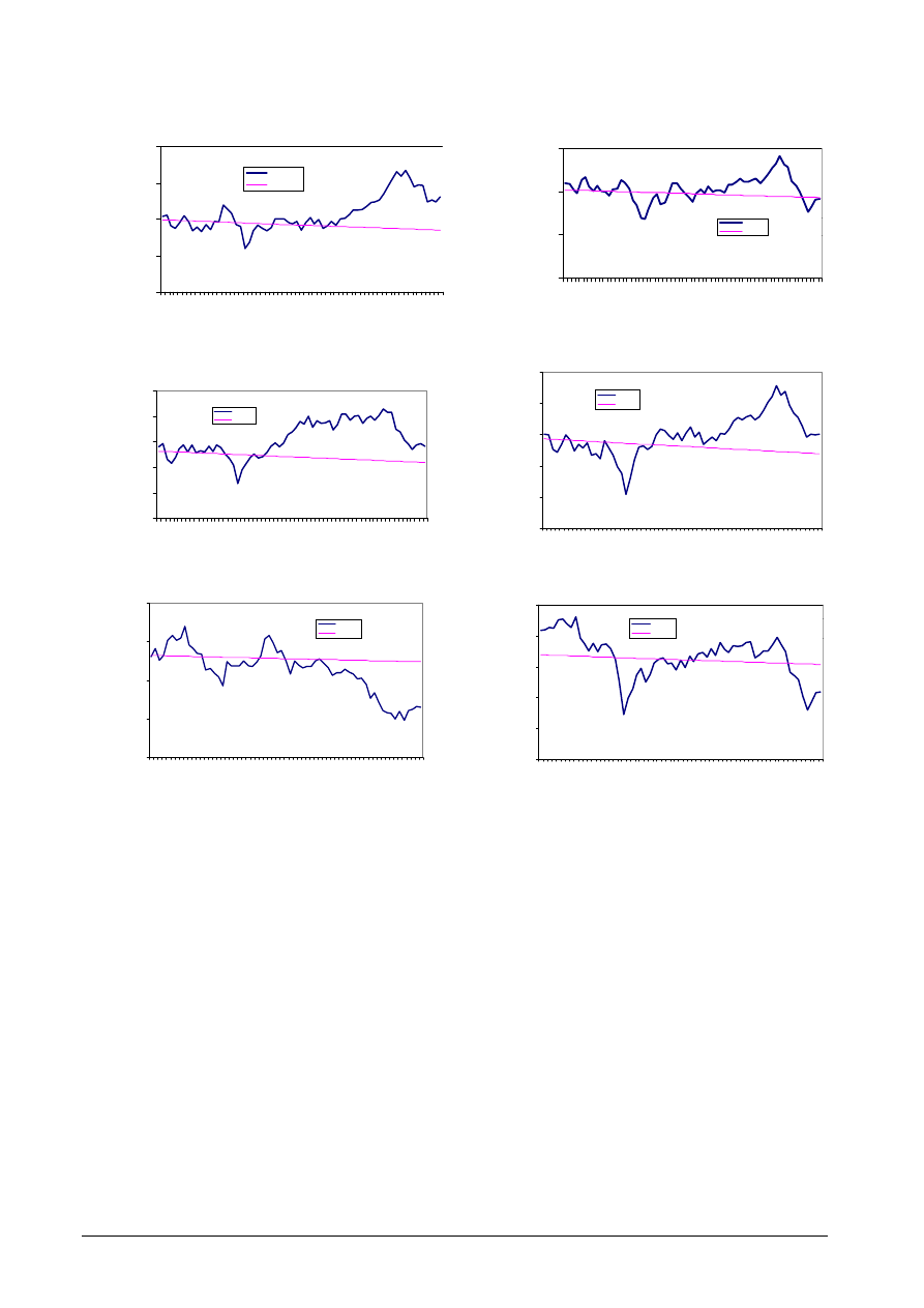
From Figures 5, 6 and 8, it is clear that the
quality of forecast with ARIMA model
deteriorates with the increase of the number
of periods for the forecasting (/testing)
phase. In other words, ARIMA could be
suitable for shorter term forecasting than
longer term. However, the results show that
neural network models produce better
performance than the conventional ARIMA
model for both shorter and longer term
forecasting which means ANN is more
suitable for financial modelling.

As we can see in Figure 5 and 6, both SCG
and BPR forecasts are better than SBP in
terms of all metrics. In our experiment this
is consistently observed in all other
currencies also. In terms of the most
commonly used criteria, i.e., NMSE and
MAE, SCG perform better than BPR in all
currencies except Japanese Yen. In terms
indicator DS, SCG yields slightly better
performance in case of Swiss France, BPR
slightly better in US Dollar and British
Pound, both perform equally in case of
Japanese Yen, Singapore and New
Zealand Dollar. Although we reported only
the best predictions in this paper, a sample
outputs based on error indicator NMSE for
the best and worst predictions produced by
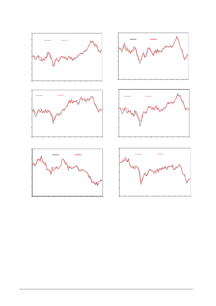
SBP for British-Pound are shown in Figure
7. The actual and forecasted time series of
six currency rates using ARIMA, and SCG
model are shown in Figures 8 and 9
respectively. From Figures 5 and 6, one can
easily imagine the superiority of ANN based
models over ARIMA.

0.33

0.34

0.35

0.36

0.37

0.38

0.39

1

5

9 13 17 21 25 29 33 37 41 45 49 53 57 61 65

Week

MNS

E

Actual

Predict-SBP(best)

Predict-SBP(worst)

Figure 7. Sample worst and best predictions

Conclusion

In this study, we investigated three ANN
based forecasting models to predict six
foreign currencies against Australian dollar
using historical data and moving average
technical indicators, and a comparison was
made with traditional ARIMA model. All the

ANN based models outperformed ARIMA
model measured on three different
performance metrics. Results demonstrate
that ANN based model can forecast the
Forex rates closely. Among the three ANN
based models, SCG based model yields
best results measured on two popular
metrics and shows results comparable to
BPR based models when measured on the
indicator DS.


References

[1] G. E. P. Box and G. M. Jenkins, Time
Series Analysis: Forecasting and Control,
Holden-Day, San Francosco, CA.

[2] L. Cao and F. Tay, “Financial
Forecasting Using Support Vector
Machines,” Neural Comput & Applic, vol.
10, pp.184-192, 2001.

[3] G. Deboeck, Trading on the Edge:
Neural, Genetic and Fuzzy Systems for
Chaotic Financial Markets, New York Wiley,
1994.

[4] F. D. Foresee and M.T. Hagan, “Gauss-
Newton approximation to Bayesian
regularization,” Proc. IJCNN 1997, pp.
1930-1935.

[5] M.T. Hagan, H.B. Demuth and M.H.
Beale, Neural Network Design, PWS
Publishing, Boston, MA, 1996.

[6] J. Hanke and A. Reitsch, Business
Forecasting, Allyn and Bacon, Inc., Boston,
1986.

[7] T. Hill, M. O’Connor and W. Remus,
“Neural Network Models for Time Series
Forecasts,” Management Science, vol. 42,
pp 1082-1092, 1996.

[8] H. B. Hwarng and H. T. Ang, “A Simple
Neural Network for ARMA(p,q) Time
Series,”

OMEGA: Int. Journal of

Management Science, vol. 29, pp 319-333,
2002.

[9] J. Jarrett, Business Forecasting
Methods, Basil Blackwell, Oxford, 1991.

[10] W. C. Jhee and J. K. Lee,
“Performance of Neural Networks in
Managerial Forecasting,” Intelligent
Systems in Accounting, Finance and
Management, vol. 2, pp 55-71, 1993.

ASOR BULLETIN, Volume 22 Number 2, June 2003 9

[11] I. Kaastra and M. Boyd, “Designing a
Neural Network for Forecasting Financial
and Economic Time-Series,”
Neurocomputing, vol. 10, pp215-236, 1996.

[12] B. D. Klein and D. F. Rossin, “Data
Quality in Neural Network Models: Effect of
Error Rate and Magnitude of Error on
Predictive Accuracy,” OMEGA: Int. Journal
of Management Science, vol. 27, pp 569-
582, 1999.

[13] B. LeBaron, “Technical trading rule
profitability and foreign exchange
intervention,” Journal of Int. Economics, vol.
49, pp. 124-143, 1999.

[14] D.J.C. Mackay, “Bayesian
interpolation,” Neural Computation, vol. 4,
pp. 415-447, 1992.

[15] A.F. Moller, “A scaled conjugate
gradient algorithm for fast supervised
learning,” Neural Networks, vol. 6, pp.525-
533, 1993.

[16] D.E Rumelhart, J.L. McClelland and the
PDP research group, Parallel Distributed
Processing, vol. 1, MIT Press, 1986.

[17] Z. Tang and P. A. Fishwich, “Back-
Propagation Neural Nets as Models for
Time Series Forecasting,” ORSA Journal on
Computing, vol. 5(4), pp 374-385, 1993.

[18] J. H.Wang and J. Y. Leu, “Stock Market
Trend Prediction Using ARIMA-based
Neural Networks,” Proc. of IEEE Int. Conf.
on Neural Networks, vol. 4, pp. 2160-2165,
1996.

[19] S. Wang (1998) An Insight into the
Standard Back-Propagation Neural Network
Model for Regression Analysis, OMEGA:
Int. Journal of Management Science, 26,
pp133-140.

[20]J. Yao, Y. Li and C. L. Tan, “Option
Price Forecasting Using Neural Networks,”
OMEGA: Int. Journal of Management
Science, vol. 28, pp 455-466, 2000.

[21] J. Yao and C.L. Tan, “A case study on
using neural networks to perform technical
forecasting of forex,” Neurocomputing, vol.
34, pp. 79-98, 2000.

[22] S. Yaser and A. Atiya, “Introduction to
Financial Forecasting,“ Applied Intelligence,
vol. 6, pp 205-213, 1996.

[23] G. Zhang and M. Y. Hu, “Neural
Network Forecasting of the British
Pound/US Dollar Exchange Rate,” OMEGA:
Int. Journal of Management Science, 26, pp
495-506, 1998.

10 ASOR BULLETIN, Volume 22 Number 2, June 2003

0.44

0.48

0.52

0.56

0.6

1

11

21

31

41

51

61

Actual

Forecast

(a) USD/AUD

0.28

0.32

0.36

0.4

1

11

21

31

41

51

61

A ctual

Forecast

(b) GBP/AUD

50

55

60

65

70

75

1

11

21

31

41

51

61

A ctual

Forecast

(c) JPY/AUD

0.8

0.85

0.9

0.95

1

1.05

1

11

21

31

41

51

61

A ctual

Forecast

(d) SGD/AUD

1.1

1.15

1.2

1.25

1.3

1

11

21

31

41

51

61

A ctual

Forecast

(e) NZD/AUD

0.7

0.75

0.8

0.85

0.9

0.95

1

11

21

31

41

51

61

A ctual

Forecast

(f) CHF/AUD

Figure 8. Forecasting of different currencies by ARIMA model over 65 weeks.

ASOR BULLETIN, Volume 22 Number 2, June 2003 11

0.44

0.46

0.48

0.5

0.52

0.54

0.56

0.58

0.6

1

11

21

31

41

51

61

Actual

Forecast

50

55

60

65

70

75

1

11

21

31

41

51

61

Actual

Forecast

0.8

0.85

0.9

0.95

1

1.05

1

11

21

31

41

51

61

Actual

Forecast

0.3

0.31

0.32

0.33

0.34

0.35

0.36

0.37

0.38

0.39

0.4

1

11

21

31

41

51

61

Actual

Forecast

1.1

1.14

1.18

1.22

1.26

1.3

1

11

21

31

41

51

61

Actual

Forecast

0.7

0.75

0.8

0.85

0.9

0.95

1

1

11

21

31

41

51

61

Actual

Forecast

(a) USD/AUD

(b) GBP/AUD

(c) JPY/AUD

(d) SGD/AUD

(e) NZD/AUD

(f) CHF/AUD

Figure 9. Forecasting of different currencies by SCG based neural network model over 65 weeks.