1

Advanced mathematics

for budgets

Chapter

2

2

2.1

Forecasting techniques

Forecasting methods budget, forecast or project by extending historical data into the future,
the various techniques include:



High-low technique



The ‘line of best fit’ using human judgement



Regression analysis (or ‘least squares method’)



Time series

In this chapter we will look at “regression analysis” and “time series” only as we have
already looked at high-low technique” and “line of best for” in an early chapter.

All the above methods normally focus on creating a linear relationship for sales or cost
forecasting, normally expressed as;

Y= a + bX

Once a trend can be found by using the above methods, this linear forecasting function can be
used in order to forecast for other activity levels. Interpolation is when you are estimating an
activity; within the given range of the data, you would have used to produce the trend with.
This is more likely to be accurate than ‘extrapolation’ techniques, which is estimating outside
of the given range of data you have.

Note: using historical information may not always be a good guidance for forecasting the
future.

2.2

Regression analysis (or ‘least squares method’)

Regression analysis (or ‘method of least squares’) uses a formulae (provided in the exam) in
order to calculate a more scientific ‘line of best fit’. It is therefore harder to understand,
however far more accurate. It creates a model (Y = a + bX) that can be used as a forecasting
technique.

Formulae provided in your exam

Y = a + bX

b = n∑XY – (∑X)(∑Y)
n∑X

2

– (∑X)

2

a = Y – bX

3

Example 2.1

Tastes like cac but boy does it sell Ltd, installs and fills up regularly canned vending
machines selling a whole range of fizzy pop brands in restaurant, pubs and hotels. At present
it is trying to predict sales forecasts for some new vending machines being sold in Spain and
has obtained the following information from vending machines installed in other Countries
with similar climates.

Temperature (Celsius)

Canned drinks sold per day

30

1,400

32

1,520

26

1,220

22

1,000

18

900

Using regression analysis, produce a trend or sales function, which can be used to
forecast the level of sales per day according to temperature?

Using the trend function you have produced, forecast what the level of sales will be if the
temperature was 24 or 40 degrees Celsius?

How reliable would the forecast be at 24 degrees compared to 40 degrees?


Assumptions of regression analysis

1. Assumes a linear relationship (this can be tested by reliability methods such as

correlation coefficient, discussed below, whereby close to one would indicate a
perfect linear relationship).

2. Generally interpolation is more accurate than extrapolation as it is looking at data that

has occurred as opposed to data that has never occurred.

3. Relies on historical information which is sometimes no guidance to the future.
4. Assumes there is an actual relationship between X and Y whereby it maybe just a

coincidence.

Correlation coefficient measures the strength of the relationship between X and Y, always
giving a value between the range between -1 and +1, indicating how perfect your relationship
is between X and Y and also whether the relationship is a positive or negative one.

The formula is not given in the exam (however correlation is not specifically mentioned in
your syllabus) but is very similar to the regression formulae just used.

Correlation coefficient (r) = n∑XY – (∑X)(∑Y)

√ ((n∑X

2

– (∑X)

2

)( n∑Y

2

– (∑Y)

2

))

4

Coefficient of determination measures how much a particular variable is determined or
explained by another. To calculate this you simply square the correlation coefficient therefore
obtaining r

2

. It will provide you with a percentage and the higher the percentage the more

determined or explained a variable is by another.


Example 2.2

Calculate the correlation coefficient for Tastes like CAC but boy does it sell Ltd, based
upon your previous calculations in example 2.1?

Calculate the coefficient of determination (r

2

) for Tastes like CAC but boy does it sell

Ltd? What does it mean?



2.3

Time series

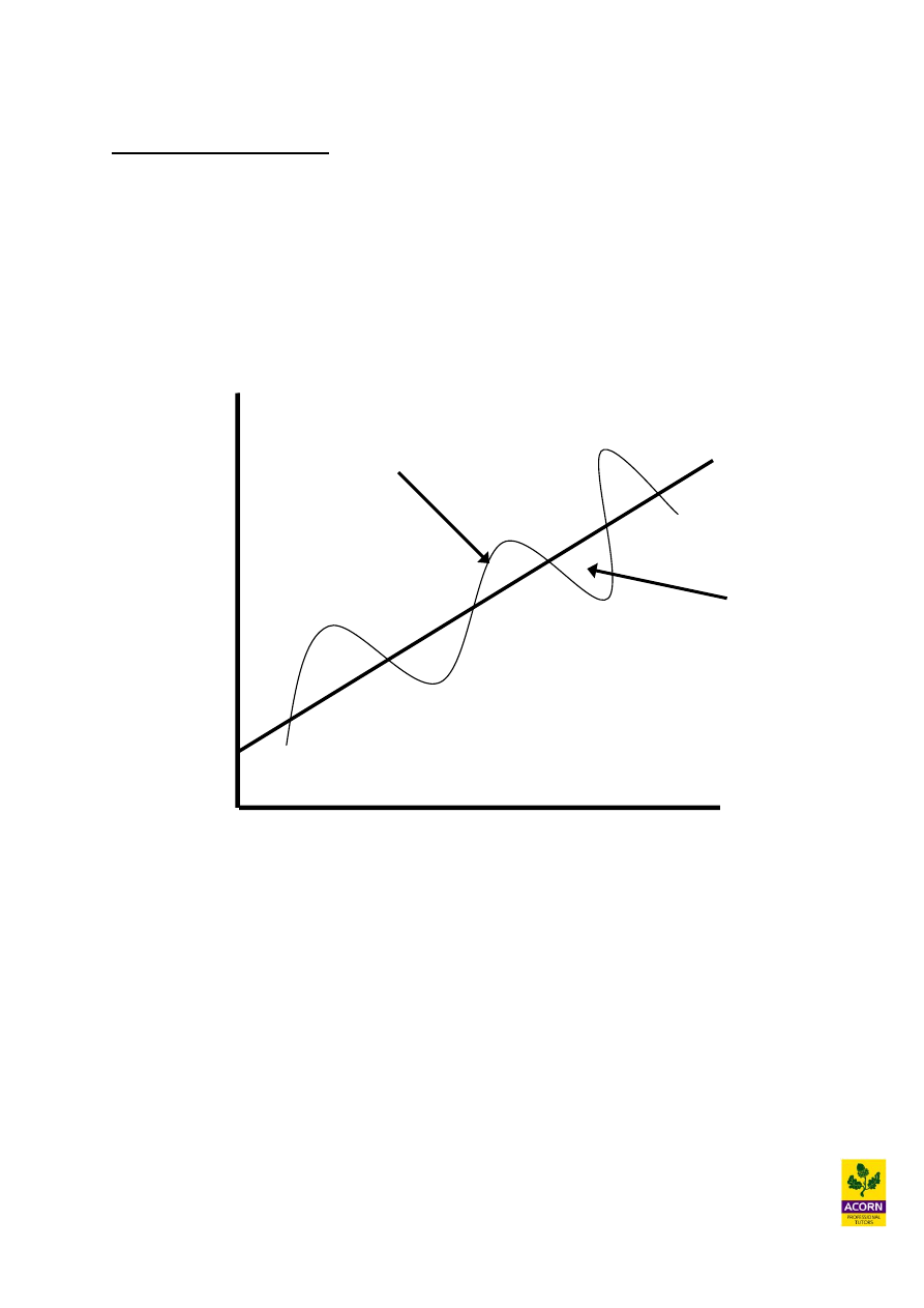
A time series is historical values recorded over time, such as total cost against output or
monthly sales against time.

The components of a time series

Trend (T)

Is the long-term movement of sales or costs over time e.g. ‘deseasonalised data’

Seasonal variations (SV)

Is the adjustment to the trend due to ‘seasonality’ in order to forecast more effectively

e.g. weather factors or the nature of the business

Cyclical variations (CV)

Is the adjustment to the trend due to the business or economic cycle

e.g. periodic booms and recessions

Random variations (RV)

Non-recurring incidents, which are uncertain events

e.g. war, technological change or severe weather or natural disasters

5

Two models for forecasting

Additive model

TS = T + (+/-) SV

Multiplicative model TS = T x SV (as a decimal or index value)

Trend (T) or Y = a + bX

You can even build into both of these models cyclical and even random variations, but exam
questions never normally have done this.

The trend and seasonal variation can be found by the technique of ‘moving averages’

If time slices are even



List vertically your time series or historical data.



Identify the ‘four point moving average’ when the time slices are even e.g. four
quarters over the year.



Find the mid-point or average of all the ‘four point moving averages’ you have

calculated, a trend can now be found and so can too any seasonal variations.



If a large number of seasonal variations exist in the same seasons within your time

series, an average would be calculated for the forecasting model.

Output

Time

SV

T

Actual data (TS)

6

If time slices are odd



List vertically your time series or historical data.



Identify the ‘three point moving average’ normally when the time slices are odd e.g.
only three periods considered in one year.



This would also be your mid-point or average you have already calculated due the

periods being odd rather than even, so a trend can now be found and so can too any
seasonal variations.



If a large number of seasonal variations exist in the same seasons within your time

series, an average would be calculated for the forecasting model.

Example 2.3

TS

‘4’ moving

T SV SV

(Ice cream sold)

average

(additive) (multiplicative)

Year 1 Qtr 1 390

Qtr 2 400

Qtr 3 500

Qtr 4 200

Year 2 Qtr 1 410

Qtr 2 450

Qtr 3 600

Qtr 4 250

Calculate a forecasting model from the above data? What would your forecast be for the
sales in Year 4 Qtr 2?

7

Example 2.4 – Worked example (CIMA past exam question)

Z plc has found that it can estimate future sales using time-series analysis and regression
techniques. The following trend equation has been derived:

y = 25,000 + 6,500x

where y is the total sales units per quarter, and x is the time period reference number.

Z has also derived the following set of seasonal variation index values for each quarter using a
multiplicative (proportional) model:

Quarter 1 = 70
Quarter 2 = 90
Quarter 3 = 150
Quarter 4 = 90

Using the above model, calculate the forecast for sales units for the third quarter of year
7, assuming that the first quarter of year 1 is time period reference number 1.

Tip : The forecast for future unit sales is expressed as

Y = a + bX

a = fixed sales regardless of the activity level (time)
b = variable sales driven by the activity level (time)
x = the activity level (time)

Y = 25,000 + 6,500X

This represents the forecast trend for unit sales. The long-term movement of sales units
forecast over time which would be ‘deseasonalised data’ and therefore must be adjusted by a
seasonalised index value of 150 (or 1.5) in order to predict accurately the number of sales
units forecast. The index value of 150 would be used because we are estimating sales for the
third quarter of year 7.

1. Work out the forecast trend for sales units

Y = 25,000 + 6,500X

Y = 25,000 + 6,500 (27 see note 1)

Y = 25,000 + 175,500

Y = 200,500 units

Note 1
(6 years x 4 quarters) + 3 quarters in year 7 = 27 quarters

8

2. Adjust this for the seasonal index value of 150

200,500 x 1.5 = 300,750 units



Example 2.5

South Eastern Railway have created a trend equation for the number of passengers in a
quarter of a year to be Y = 20,000 + 1,800X.

Y = Total number of passengers in a given quarter
X = The time period (Year 1 Qtr 1 X= 1, Year 1 Qtr 2 X = 2 etc.)

You are also provided with the following actual data for passengers carried in the first year
(year 1).

Qtr 1 20,000
Qtr 2 25,500
Qtr 3 28,800
Qtr 4 19,000

Using the multiplicative model, estimate the number of passengers to be carried in the
first quarter of year 2?

9

2.4

Limiting or principle budget factors

A limiting factor or principle budget factor means you do not have enough of a resource of
some kind, in order to produce or sell all you would like, it is a scarce resource, which is in
short supply that would cause this. The analysis would maximise contribution for an
organisation, by allocating the scarce resource to producing goods, which earn the highest
amount of contribution per unit of scarce resource available.

Examples of limiting factors



Shortages in demand



Shortages in material



Shortages in labour hours



Shortages in machine hours



Shortages in money

Method for limiting factor analysis



Identify the limiting factor – This is that resource which is scarce and the aim being

to produce until the limiting factor is fully utilised. Examples of this are labour or
materials.



Contribution per unit – Calculate contribution for each of the products that are

being manufactured which use the limiting factor. Contribution is sales less variable
costs.



Limiting factor used in each product – Calculate how much of the limiting factor is

used in the manufacture of each product.



Contribution per unit of limiting factor – Calculate how much contribution is

earned per unit of the limiting factor used in the production of each product. To work
this out we simply divide the contribution per unit by the limiting factor used in each
product.



Rank - In order of highest contribution per unit of limiting factor, and then

manufacture that product which yields the most contribution per limiting factor first,
then the next highest after demand has been met on the first. This should continue
until all the limiting factor resource has been used.

Contribution per unit =

Sales price per unit less all variable cost per unit (it ignores all fixed cost).

10

Contribution earned per unit of scarce resource =

Contribution per unit

Number of units of scarce resource required in order to produce it

Example 2.6 – Worked example (CIMA past exam question)

The following details relate to ready meals that are prepared by a food processing company:

Ready meal

K

L

M

$/meal

$/meal

$/meal

Selling price

5

3

4.40

Ingredients

2

1

1.30

Variable conversion costs

1.60

0.80

1.85

Fixed conversion costs

0·50

0·30

0·60

Profit

0·90

0·90

0·65

Oven time (minutes per ready meal)

10

4

8

Each of the meals is prepared using a series of processes, one of which involves cooking the
ingredients in a large oven. The availability of cooking time in the oven is limited and,
because each of the meals requires cooking at a different oven temperature, it is not possible
to cook more than one of the meals in the oven at the same time.

The fixed conversion costs are general fixed costs that are not specific to any type of ready
meal.

Rank in terms of the profitability of the manufacture of these meals.

They have identified that cooking time is our limiting factor and so we need to work out
contribution per minute of cooking time and then rank them in order of profitability.

Meal

K

L

M

Selling price

$5

$3

$4.40

Ingredients

($2)

($1)

($1.30)

Variable conversion costs

($1.60)

($0.80)

($1.85)

Contribution

$1.40

$1.20

$1.25

Cooking time per meal

10

4

8

Contribution per minute

$1.40/10 = $0.14

$1.20/4 = $0.30

$1.25/8 = $0.16

Rank

3

1

2

11

Example 2.7

Cosmetics R Us Plc do 3 forms of cosmetic surgery, which are face jobs, gut tucks and lipo
suctions.

Estimated demand

FJ

GT

LS

In 1 year

10,000

2,000

3,000

Average consultancy fee

£3,000

£1,500

£2,000

Surgeon cost
(£500 per hour)

£1,500

£250

£750

Variable overhead per operation

£600 £100

£300

Fixed overhead will be £750,000 a month. Unfortunately due to most surgeons working
within this field only wanting to work within the NHS, Cosmetics R Us can only employ 20
consultants working only a 42 week year for 5 days a week, each surgeon willing to perform
operations for up to 40 hours a week.

Prepare calculations showing the number of each of the operations that Cosmetics R Us
must perform in order to maximise contribution? What would be the profit earned for
the period?

Example 2.8

What if you were told that because of high competition, there is pressure on waiting lists
for FJs and therefore Cosmetics R Us must fulfil all operations on FJ first?

12

2.5

Break even analysis or cost volume profit (CVP) analysis

Cost-volume-profit (CVP) analysis looks at how profit changes when there are changes in

variable costs, sales price, fixed costs and quantity.

It is a good example of “what if?” analysis and it in particular looks at sales minus variable
costs which is known as contribution. It allows management to understand the level of sales
needed to cover all costs of a project and what level of sales is needed start making profits.

To break even would mean an organisation would be earning no profit and no loss.

Sales revenue = All variable and fixed cost

Main assumptions in this model are that selling price, fixed costs and variable costs are
constant.

Formulae to learn

Contribution per unit = sales price per unit less variable cost per unit

Break-even volume = Fixed overhead
Contribution per unit

The number of units you would need to sell in order to earn enough contribution to cover the
fixed overhead e.g. the number of units sold where the contribution would equal the fixed
overhead.

The contribution to sales ratio (C/S ratio)

The contribution to sales (or C/S) ratio (also called the profit-volume or P/V ratio) would
calculate how much contribution a product would earn for every £1 of sales generated,
expressed as a decimal or percentage. For example a 0.4 or 40% C/S ratio, would mean 40
pence of contribution is earned for every £1 of sales generated.

C/S ratio =

Contribution per unit

Sales price per unit

C/S ratio = Total contribution
Total sales revenue

13

Break-even revenue

The sales revenue earned that would give no profit and no loss. It can be calculated by
multiplying the break-even volume (above) by the products selling price, or alternatively by
using the following formulae.

= Fixed overhead
C/S ratio

Margin of safety

Measures the sensitivity of the budgeted sales volume compared with the break-even sales
volume. The difference between the level of sales activity achieved and the level of sales
activity required to break-even in absolute or percentage terms.

Margin of safety (units) = Budgeted sales volume less Break-even sales volume

Margin of safety (%) = Budgeted sales less Break-even sales volume x 100

Budgeted sales volume

Number of units sold to achieve a target profit

= Fixed cost + Target profit
Contribution per unit

14

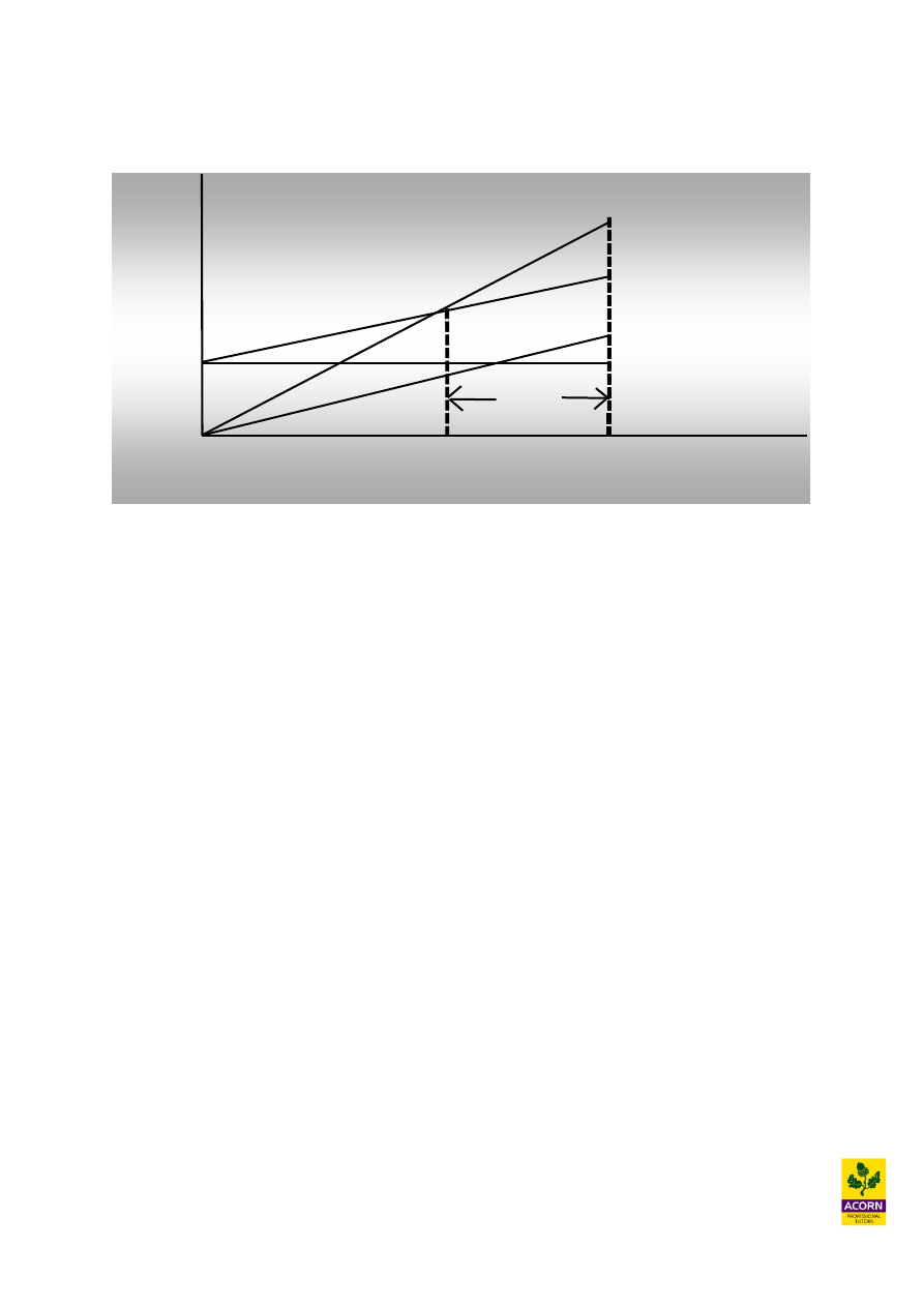
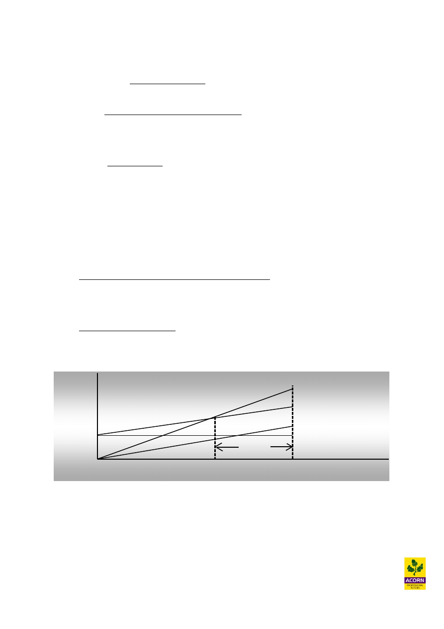
Break-even charts

Indicates graphically profit and losses at different levels of sales volume achieved.

Output (units)

Margin

of

safety

Budgeted

or actual

sales

Break-

even

point

Sales

revenue

Total

costs

Variable costs

Fixed costs

Cost and

revenue £

0



Where sales revenue is greater than total cost it means that profits are being

generated.



Where sales revenue is less than total cost it means that losses are being incurred.



Where sales revenue equals total costs (intersection of the sales revenue line and total

costs line) it means that no profit or loss is occurring. This is the break-even point.



Variable costs vary directly with output, as more output is produced then more

variable costs are incurred.



Fixed costs do not vary with output and are constant for a range of output produced.

They are incurred even when there is no output at the beginning of production. This is
because they are costs that must be incurred to support manufacture such as
machinery or a warehouse.



The total costs line is a representation of the combined variable and fixed costs. This

is why at nil output it has a cost which represents fixed costs, and then as output
increases the total cost line varies with it and in parallel with the variable cost line.



The margin of safety is the extra amount of sales that is expected to be generated

when the budget or actual sales is compared to the break-even level of sales.

15

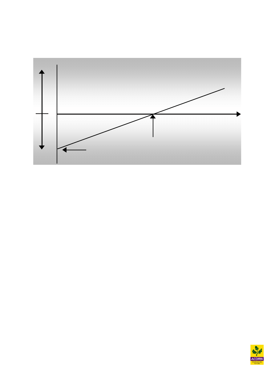
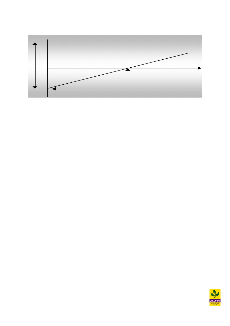
Profit volume charts

A variation of a break-even chart, indicating graphically the relationship between profit and
losses at different levels of sales volume achieved.

Loss = fixed

costs at zero

sales activity

Break-

even

point

Sales

Loss

£

£

Profit

0

The profit volume chart is a summarisation of the break even chart, whereby the line
represents total profit (sales less all costs). When the line rises above the horizontal axis it
means that production is beginning to yield a profit, before this point it means that production
is yielding a loss. The break-even point where no profit or loss is being made is where this
profit line intersected the horizontal axis.

Assumptions

1. Single product or single mix of products
2. Fixed cost, variable cost and selling price are constant
3. The level of production will equal the level of sales

16

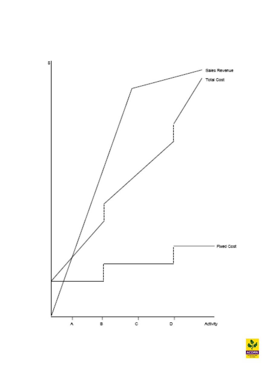
Example 2.9 – (CIMA past exam question)

Diagram showing costs and revenues over a range of activity levels

17

You are required to interpret the diagram and explain how it illustrates issues that the
operational managers should consider when making decisions. (Note: your answer
must include explanations of the Sales Revenue, Total Cost and Fixed Cost lines, and
the significance of each of the activity levels labelled A, B, C, D).

Example 2.10

Z-Boxes sell for £299 and their variable production cost is £99. The research and
development, and fixed production overheads for the year are £1.2 million.

a) Calculate the break-even level of sales volume and revenue?
b) Calculate the break-even revenue using C/S ratio?
c) The budget revenue is £2.99 million; calculate the margin of safety in units and as

a percentage?

d) Produce a break-even chart and profit-volume chart using the information

above?

e) How many Z-Boxes must be sold to achieve £500,000 profit

18

2.6

Multiple product scenarios

Break-even analysis can also be used to work out either a break-even volume or revenue,
given a multiple product scenario. This is achieved using the ‘average contribution per unit’
or ‘average C/S ratio per unit’ for all products together.

This calculation will only work providing the sales mix remains constant. Change the
mix and the C/S ratio or contribution per unit of the mix of the products will change; hence
you would need to again work out the break-even volume or revenue.


Example 2.11

Me ole cock spaniel plc makes 3 products, details as follows:

Apples (£) Pears (£) Cockneys (£)

Selling price

60

80

40

Variable cost

(20)

(30)

(20)

Contribution

40

50

20

Sales (units)

2,000

3,000

5,000

Fixed overhead for the year £800,000

Calculate the break-even level of sales?






Example 2.12 – (CIMA past exam question)


A company provides a number of different services to its customers from a single office. The
fixed costs of the office, including staff costs, are absorbed into the company’s service costs
using an absorption rate of $25 per consulting hour based on a budgeted activity level of
100,000 hours each period.

Fee income and variable costs are different depending on the services provided, but the
average contribution to sales ratio is 35%.

Calculate the breakeven fee income?

19

Key summary of chapter

Regression analysis (or ‘method of least squares’) uses a formulae (provided in the exam) in
order to calculate a more scientific ‘line of best fit’. It is therefore harder to understand,
however far more accurate. It creates a model (Y = a + bX) that can be used as a forecasting
technique.

Formulae provided in your exam

Y = a + bX

b = n∑XY – (∑X)(∑Y)
n∑X

2

– (∑X)

2

a = Y – bX

Correlation coefficient measures the strength of the relationship between X and Y, always
giving a value between the range between -1 and +1, indicating how perfect your relationship
is between X and Y and also whether the relationship is a positive or negative one.


Correlation coefficient (r) = n∑XY – (∑X)(∑Y)

√ ((n∑X

2

– (∑X)

2

)( n∑Y

2

– (∑Y)

2

))

Coefficient of determination measures how much a particular variable is determined or
explained by another. To calculate this you simply square the correlation coefficient therefore
obtaining r

2

. It will provide you with a percentage and the higher the percentage the more

determined or explained a variable is by another.

Time series

A time series is historical values recorded over time, such as total cost against output or
monthly sales against time.

Two models for forecasting

Additive model

TS = T + (+/-) SV

Multiplicative model TS = T x SV (as a decimal or index value)

Trend (T) or Y = a + bX

A limiting factor or principle budget factor means you do not have enough of a resource in
order to produce or sell all you would like.

20

Method for limiting factor analysis



Identify the limiting factor



Contribution per unit



Limiting factor used in each product



Contribution per unit of limiting factor



Rank

Contribution per unit =

Sales price per unit less all variable cost per unit (it ignores all fixed cost).

Contribution earned per unit of scarce resource =

Contribution per unit

Number of units of scarce resource required in order to produce it

Break even analysis or cost volume profit (CVP) analysis

Cost-volume-profit (CVP) analysis looks at how profit changes when there are changes in

variable costs, sales price, fixed costs and quantity.

Formulae to learn

Contribution per unit = Sales price per unit less variable cost per unit

Break-even volume = Fixed overhead
Contribution per unit sold

21

Contribution to Sales ratio (C/S ratio)

= Contribution per unit
Sales price per unit

or = Total contribution from a product sold
Total sales revenue earned from a product sold

Break-even revenue

=

Fixed overhead

C/S ratio

or = Break-even volume x Sales price per unit sold

Margin of safety (units)

= Budgeted sales volume less Break-even sales volume

Margin of safety (%)

= Budgeted sales volume less Break-even sales volume x 100

Budgeted sales

Number of units sold to achieve a target profit

= Fixed cost + Desired profit
Contribution per unit

Break-even charts

Output (units)

Margin

of

safety

Budgeted

or actual

sales

Break-

even
point

Sales revenue

Total costs

Variable costs

Fixed costs

Cost and

revenue £

0

22

Profit volume charts:

Loss = fixed

costs at zero

sales activity

Break-

even

point

Sales

Loss

£

£

Profit

0

23

Solutions to lecture examples

24

Chapter 2

Example 2.1

Temperature is the independent variable as the number of cans that are sold is determined by
how hot it is on a given day. Therefore temperature is the “X” variable, and so number of
cans sold must be the “Y” variable.

Temperature (X)

X²

Drinks sold (Y)

XY

30

900

1,400

42,000

32

1,024

1,520

48,640

26

676

1,220

31,720

22

484

1,000

22,000

18

324

900

16,200

128

3,408

6,040

160,560

“∑” means sum of or total, so therefore:

∑x = 128, ∑y = 6,040, ∑x² = 3,408, (∑x)² = 128² = 16,384, ∑xy = 160,560

b = n∑XY – (∑X)(∑Y)
n∑X

2

– (∑X)

2

n = the number of data items

Therefore:

b = 5(160,560) – (128)(6,040)
5(3,408) – 16,384

b = 802,800 – 773,120
17,040 – 16,384

b = 29,680
656

b = 45 cans sold for every degree increase in temperature (rounded to the nearest can)

25

__ __
a = Y – bX
__
Y = average or mean of Y = 6,040 / 5 = 1,208
__
X = average or mean of X = 128 / 5 = 25.6

a = 1,208 – (45 x 25.6)

a = 56 cans sold regardless of temperature

Y = 56 + 45X

Forecast for 24 degrees 56 + 45(24) = 1,136 cans sold

Forecast for 40 degrees 56 + 45(40) = 1,856 cans sold

Forecasting within the range e.g. interpolation (24 degrees) should be more accurate than
extrapolation e.g. outside the range (40 degrees), as an example what if 40 degrees is far
too hot for any tourist to go out from their villa, not many drinks would be sold if this was the
case.



Example 2.2

Correlation coefficient

= 0.989

Co efficiency of determination

= 0.989

2

=0.978

Therefore 97.8% of the change in sales is caused by the change in temperature; this I
would say is a fairly reliable forecasting method to use.

26

Example 2.3

TS

‘4’ moving

T

SV

SV

(Ice cream sold)

average

(additive) (multiplicative)

SV = TS-T SV = TS/T

Year 1 Qtr 1 390

Qtr 2 400

372.5

Qtr 3 500

375.0

+125

1.333

377.5

Qtr 4 200

383.75

-183.75

0.521

390.0

Year 2 Qtr 1 410

402.5

+7.5

1.018

415.0

Qtr 2 450

421.25

+28.75

1.068

427.5

Qtr 3 600

Qtr 4 250

The seasonal variations above, give a seasonal variation for each quarter e.g. quarter one will
always be adjusted by +7.5 or 1.018 within the forecasting model. Should you have more
than one seasonal variation for each quarter then find an average and use this instead.

The trend as a base year begins in year 1 Qtr 3 at 375, it moved from 375 to 421.25 in ‘3
movements’ so for forecasting purposes (421.25-375)/3 movements = 15.4 increase in your
forecasting model for each future quarter you are predicting for (starting at 375 in year 1 Qtr
3.

Therefore using the additive model as an example the trend would be Y = 375 + 15.4X

Where Y is the trend and X the quarter (Yr 1 Qtr 4 = 1, Yr 2 Qtr 1 = 2, Yr 2 Qtr 2 = 3…and
so on). Once the trend has been found this is then adjusted for the seasonal variation by
multiplying or adding, depending on what model you are using.

So using the additive model to predict Year 4 Qtr 2:

Y = 375 + 15.4(11)
Y = 544.4

544.4 + 28.75 = 573 units forecast for this period.

27

Example 2.5

South Eastern Railway

TS

T

SV = TS/T

20,000

21,800

0.92

25,500

23,600

1.08

28,800

25,400

1.13

19,000

27,200

0.69

SV do not need to be averaged as you only have the first years SV anyway for each quarter.

Year 2 Qtr 1 20,000 + 1,800(5) x 0.92 = 26,680 forecast for the number of passengers.

28

Example 2.7

FJ

GT

LS

Number of hours per operation

3

0.5

1.5

Contribution per operation (£)

900

1,150

950

Contribution per LF
(Operating hours)

300

2,300

633

RANKING

3

rd

1

st

2

nd

They should perform

1

st

GT 0.5 Hrs x 2,000 max demand =

1,000 Hrs

2

nd

LS 1.5 Hrs x 3,000 max demand =

4,500 Hrs

3

rd

(28,100 Hrs remaining/3 Hrs an operation

9,367 operation performed x 3 Hrs =

28,100 Hrs

33,600 Hrs

Budgeted profit will be about £4.58 million

£000s

FJ 9,367 x (3,000 - 2,100) =

8,430.3

GT 2,000 x (1,500 - 350) =

2,300.0

LS 3,000 x (2,000 - 1,050) =

2,850.0

Contribution

13,580.3

Fixed cost (750 x 12 months)

(9,000)

Profit

4,580.3

An alternative method could have been used above. Calculation of contribution could have
been worked out on the basis of surgeon hours x contribution per hour for each product

29

Example 2.8


FJs (NO CHOICE) 10,000 x 3 Hrs =

30,000

GT 2,000 x 0.5 Hrs (most profitable next)

1,000

LS 2,600 Hrs (balance) / 1.5 Hrs = 1,733 operations
x 1.5 Hrs

2,600

33,600

If you produce a budget now, the profit would be lower, as less profitable FJs are being
substituted for more profitable LS.

Example 2.9 – (CIMA past exam question)

Explanation of sales revenue line

The sales revenue line shows the amount of sales earned throughout the different level of
activities. It can be seen that between zero and somewhere between activity B and C there is a
constant rise or straight line increase in sales revenue. This means that the unit price charged is
the same and volume sold has been increasing at a constant rate.

Beyond the point between B and C sales revenue increases at a much slower rate, this indicates
that selling price per unit is too high and in order to achieve previous rates of growth there has
to be a reduction in unit price.

Explanation of the fixed cost line

A fixed cost is a cost which cannot be easily identified or related to a cost per unit or
activity of any kind e.g. a cost which remains constant when the production of a good or
service within the organisation rises or falls.

Fixed cost over the long-term will normally display the characteristics of ‘stepped’ cost
behaviour. That is the cost remains constant but only within a certain range of production.
Once this range of production is exceeded the fixed cost will rise.

In the diagram we can see that the fixed cost line is stepped. Between the zero activity and up
to activity level B fixed costs are constant. At zero activity fixed costs need to be spent such as
machinery and buildings in order to manufacture products.

If we were to increase our level of activity beyond level B there needs to be an increase in
fixed costs and then the costs are constant up to activity level D. There is another increase in
fixed costs at activity D when looking beyond this point and then the costs are constant again.

30

These sudden stepped increases in fixed costs could be due to the factory reaching full
capacity and then extra leasehold expenses will need to be incurred in order to obtain more
buildings, if production is to increase or expand further.

Another example is supervisor’s salaries, they could be paid fixed salaries, but supervision
is limited to how many workers that can be supervised. Once the size of the workforce
exceeds a certain range another supervisor will need to be employed.

Explanation of the total cost line

Total costs include both fixed costs and variable costs. Variable costs are costs that can be
easily identified or related to a cost per unit or activity level of some kind e.g. a cost
which rises or falls directly with the production/provision of a good or service within an
organisation. Examples could include labour piece work schemes e.g. a factory worker
that gets paid for each unit they make or the cost of material/components for the
production or assembly of a product.

All variable cost starts from the origin of the graph indicating the cost is nil if the activity
level is zero. Variable cost does not necessarily behave in a linear manner e.g. a constant
amount incurred for each unit of activity. It can behave in a curvilinear (non-linear)
manner as well, in which case the variable cost line would be curved not straight.

In the diagram it can be seen that at activity zero total cost is equal to fixed costs. At this
point there are no variable costs as there is no activity only fixed costs. Between activity
levels zero and B we can see that total cost line is increasing at constant level. The constant
increase is due to variable costs being incurred as a result of increasing activity.

Total costs increases in a stepped fashion at activity levels B and D because of the costs
behaviour of fixed costs as mentioned previously. It can be seen that variable costs are
increasing at the same constant rate within total costs up to activity level D, after this point
it can be seen that the total costs line increases more steeply. This is due to increased
variable costs per unit.

Issues to consider when making decisions

At activity level A it can be seen from the diagram the sales revenue line intersects the
total cost line indicating that this is the point when the company makes no loss or profit i.e.
breakeven. Any activity beyond this point sales revenue will exceed total costs causing the
company to make a profit, and anything below this activity, total costs will exceed sales
revenue causing the company to make losses.

After activity level B fixed costs will increases sharply because of perhaps new investment
required in the manufacturing process and profits will be reduced compared to just before
activity level B. The operational mangers needs to consider whether the sales revenue
forecast is likely to hold true, if not then profits can be reduced significantly as a result of
this investment.

31

Between activity levels B and C the sales revenue line has a much higher gradient line than
total costs and the company is earning greater profits as it increases its activity. Profits are
maximised just before point C when beyond this point the sales revenue line is increasing
at a slower rate when compared to total costs.

At activity level D there is another sharp increase in fixed costs and also variable costs are
rising at steeper gradient to sales revenue. The operational manger should recommend to
the company to continue to produce activity as long as the extra revenue is greater than the
extra cost or variable cost.

32

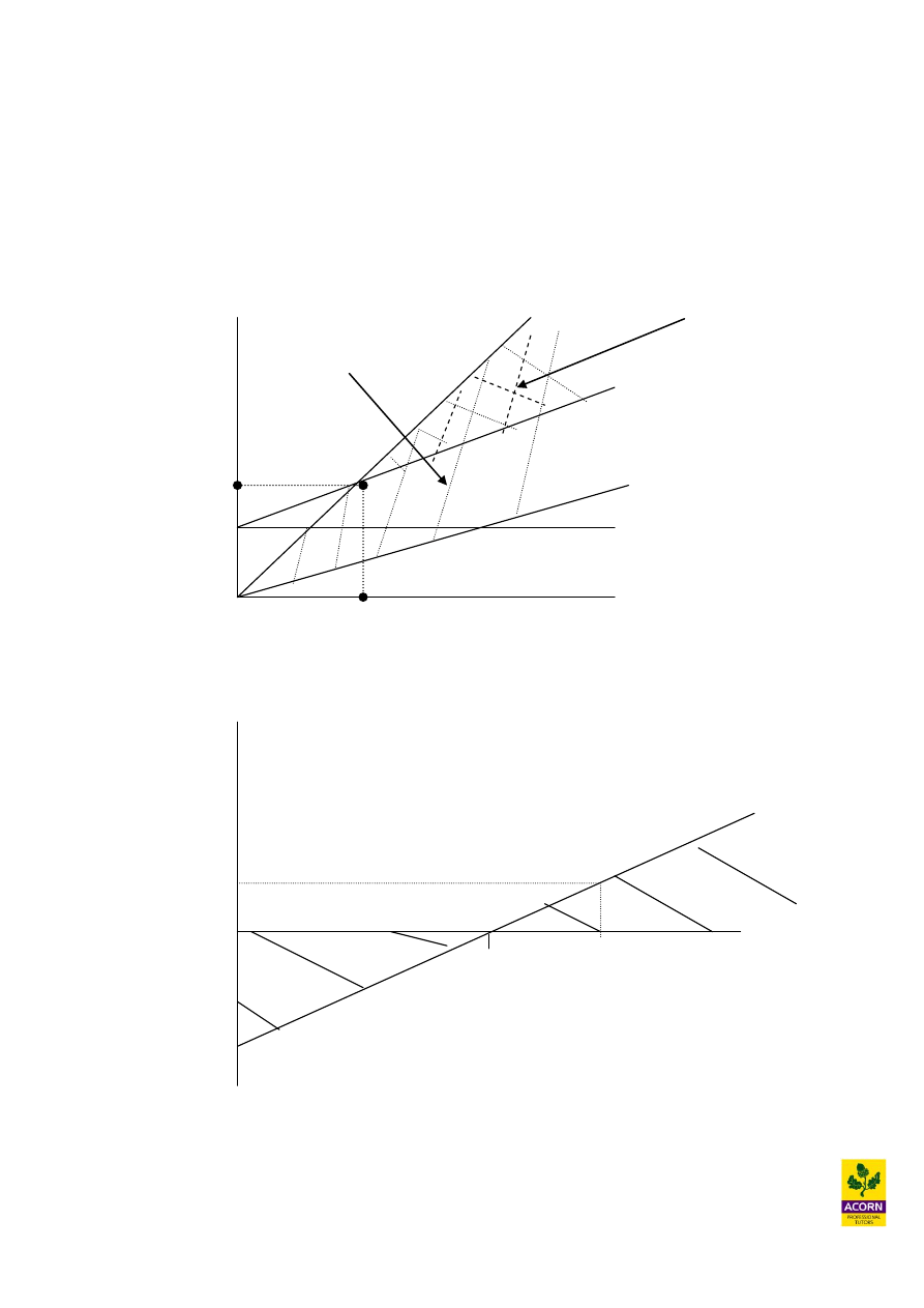
Example 2.10

a) 1.2 million/£200 = 6,000 units, 6,000 units x £299 = £1,794,000
b) £1.2 million/0.6689 = £1,793,990
c) £2.99 million/£299 = budget volume 10,000 (10,000 - 6,000 = 4,000 margin of

safety) or (4,000/10,000 = 40%)

d) See charts below

e) (1.2m + 0.5m)/£200 = 8,500 units

6,000

Fixed

Cost

Variable

cost

Sal
es

Output

£

1.794 m

Total Cost

Area of

contribution

Area of

profit

£

10,000

+ 0.8m

Output

6,000

-1.2 m

LOSS

PROFIT

Sales

33

Example 2.11

Average contribution per unit

2,000 x £40 = 80,000
3,000 x £50 = 150,000
5,000 x £20 = 100,000
Total 330,000 / 10,000 units = £33 average contribution per unit

OR 2/10 x £40 + 3/10 x £50 + 5/10 x £20 = £33 average contribution per unit

£800,000 / £33 per unit = 24,242 units sold (in the mix 2:3:5)

Break-even revenue
£
Apples 2/10 x 24,242 units sold = 4,848 x £60 = 290,880
Pears 3/10 x 24,242 units sold = 7,273 x £80 = 581,840
Cockneys 5/10 x 24,242 units sold = 12,121 x £40 = 484,840

24,242 1,357,560

Alternative method would be to use the average C/S ratio

Apples 0.666 x 0.2 =

0.133

Pears 0.625 x 0.3 =

0.1875

Cockneys 0.500 x 0.5 =

0.25

0.5705

£800,000/0.5705 = £1,402,278 (close enough to £1,357,560 above!!!)

34

Example 2.12 – (CIMA past exam question)

A company provides a number of different services to its customers from a single office.
The fixed costs of the office, including staff costs, are absorbed into the company’s service
costs using an absorption rate of $25 per consulting hour based on a budgeted activity level
of 100,000 hours each period.

Fee income and variable costs are different depending on the services provided, but the
average contribution to sales ratio is 35%.

Calculate the breakeven fee income.

Break-even revenue = Fixed overhead / C/S ratio

Therefore: $2,500,000 / 0.35 = $7,142,857