Using Spatio-Temporal Information in API Calls with
Machine Learning Algorithms for Malware Detection

Faraz Ahmed, Haider Hameed, M. Zubair Shafiq, Muddassar Farooq

Next Generation Intelligent Networks Research Center (nexGIN RC)

National University of Computer and Emerging Science (FAST-NUCES)

Islamabad 44000, Pakistan

{faraz.ahmed,haider.hameed,zubair.shafiq,muddassar.farooq}@nexginrc.org

ABSTRACT

Run-time monitoring of program execution behavior is widely
used to discriminate between benign and malicious processes
running on an end-host. Towards this end, most of the ex-
isting run-time intrusion or malware detection techniques
utilize information available in Windows Application Pro-
gramming Interface (API) call arguments or sequences. In
comparison, the key novelty of our proposed tool is the use
of statistical features which are extracted from both spatial
(arguments) and temporal (sequences) information available
in Windows API calls. We provide this composite feature set
as an input to standard machine learning algorithms to raise
the final alarm. The results of our experiments show that
the concurrent analysis of spatio-temporal features improves
the detection accuracy of all classifiers. We also perform the
scalability analysis to identify a minimal subset of API cat-
egories to be monitored whilst maintaining high detection
accuracy.

Categories and Subject Descriptors

D.4.6 [Security and Protection]: Invasive software (e.g.,
viruses, worms, Trojan horses); I.5 [Computing Method-
ologies]: Pattern Recognition

General Terms

Algorithms, Experimentation, Security

Keywords

API calls, Machine learning algorithms, Malware detection,
Markov chain

1.

INTRODUCTION

The API calls facilitate user mode processes to request a

number of services from the kernel of Microsoft Windows
operating system. A program’s execution flow is essentially

Permission to make digital or hard copies of all or part of this work for
personal or classroom use is granted without fee provided that copies are
not made or distributed for profit or commercial advantage and that copies
bear this notice and the full citation on the first page. To copy otherwise, to
republish, to post on servers or to redistribute to lists, requires prior specific
permission and/or a fee.
AISec’09,

November 9, 2009, Chicago, Illinois, USA.

Copyright 2009 ACM 978-1-60558-781-3/09/11 ...$10.00.

equivalent to the stream of API calls [2]. Moreover, the Mi-
crosoft Windows provides a variety of API

1

calls of different

functional categories – registry, memory management, sock-
ets, etc. Every API call has a unique name, set of arguments
and return value. The number and type of arguments may
vary for different API calls. Likewise, the type of return
value may also differ.

In the past, a significant amount of research has been fo-

cused on leveraging information available in API calls for
monitoring a program’s behavior. The behavior of a pro-
gram can potentially highlight anomalous and malicious ac-
tivities.

The seminal work of Forrest et al.

in [9] lever-

aged temporal information (fixed length sequences of system
calls) to discriminate between benign and malicious Unix
processes [16]. Later, Wepsi et al. proposed an improved
version with variable length system call sequences [17]. In
a recent work, the authors propose to extract semantics by
annotating call sequences for malware detection [6]. The
use of flow graphs to model temporal information of system
calls has been proposed in [5]. An important shortcoming
of these schemes is that a crafty attacker can manipulate
temporal information to circumvent detection [12], [15].

Subsequently, Mutz et al. proposed a technique that uti-

lizes information present in system call arguments and re-
turn values [11].

The results of their experiments reveal

that using spatial information enhances the robustness of
their proposed approach to mimicry attacks and other eva-
sion attempts. Another technique, M-LERAD, uses simple
white-lists of fixed-length sequences and system call argu-
ment values for anomaly detection [14]. The authors report
that the accuracy of the composite scheme is better than
either of the standalone spatial and temporal approaches.

In this paper, we propose a composite malware detection

scheme that extracts statistical features from both spatial
and temporal information available in run-time API calls
of Windows operating systems. The thesis of our approach
is that leveraging spatio-temporal information in run-time
API calls with machine learning algorithms can significantly
enhance the malware detection accuracy. Figure 1 provides
the architecture of our proposed scheme. Our tool consists
of two modules: (1) offline training module applies machine
learning algorithms on the available data to develop a train-
ing model, and (2) online detection module extracts spatio-
temporal features at run-time and compares them with the

1

The latest Microsoft Windows operating systems pro-

vide both Native API (system calls) and Windows API.
Throughout this paper, by API we refer to both of them
unless stated otherwise.

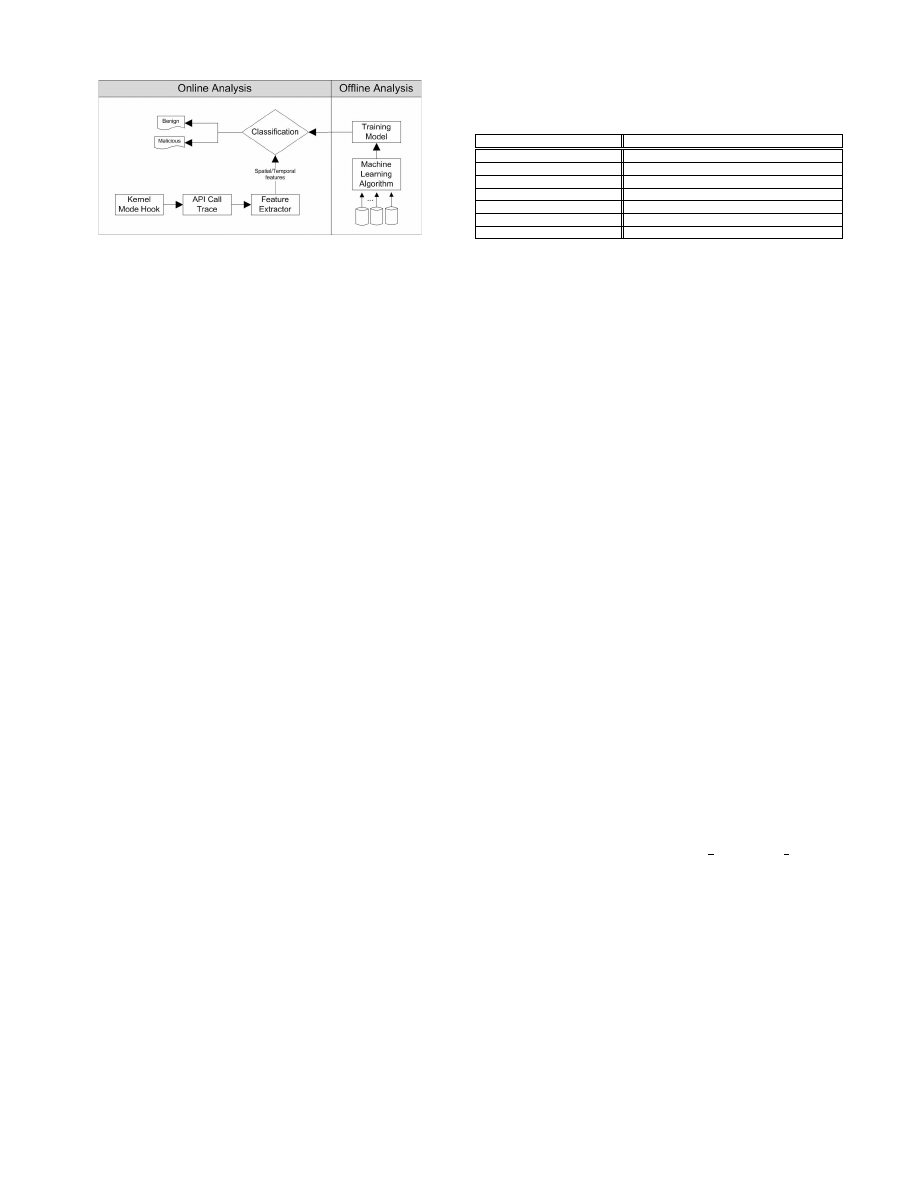
Figure 1: Block diagram of our proposed malware
detection tool

training model to classify a running process as benign or
malware.

In our scheme, spatial features are generally statistical

properties such as means, variances and entropies of address
pointers and size parameters. The temporal information is
modeled using n

th

order discrete time Markov chain with

k states, where each state corresponds to a particular API
call. In the training phase, two separate Markov chains are
constructed for benign and malicious traces that result in k

n

different transition probabilities for each chain. The less ‘dis-
criminative’ transitions are pruned by using an information-
theoretic measure called information gain (IG). Γ transi-
tions with the highest values of IG are selected as boolean
features. The extracted spatial and temporal features are
then given as input to the standard machine learning algo-
rithms for classification.

We have used a commercial API call tracer that uses the

kernel-mode hook to record the logs for running processes
on Microsoft Windows XP. To reduce the complexity of run-
time tracing, we have short-listed 237 core API calls from
six different functional categories such as socket, memory
management, processes, and threads etc. We have collected
system call logs of 100 benign programs. Moreover, we have
collected system call traces of 117 trojans, 165 viruses and
134 worms. These malware are obtained from a publicly
available collection called ‘VX Heavens Virus Collection’ [3].
The results of our experiments show that our system pro-
vides an accuracy of 0.98 on the average. We have also car-
ried out the scalability analysis to identify a minimal subset
of API categories to be monitored whilst maintaining high
detection accuracy. The results of the scalability analysis
show that monitoring only memory management and file
I/O API calls can provide an accuracy of 0.97.

The rest of the paper is organized as follows. In the next

section we provide an introduction to the Windows API. In
Section 3, we explore different design dimensions to extract
information – spatial and temporal – available in the Win-
dows API calls. In Section 4, we present the mathematical
formulation of our problem and then use it to model and
quantify spatio-temporal features. In Section 5, we present
details of our dataset, experimental setup and discuss the
results of experiments. Section 6 concludes the paper with
an outlook to our future research. We provide brief details
of machine learning classifiers in the accompanying technical
report [4].

Table 1: Categorization of API calls used in this
study

API Category

Explanation

Registry

registry manipulation

Network Management

manage network related operations

Memory Management

manage memory related functionalities

File Input/Output (I/O)

operations like reading from disk

Socket

socket related operations

Processes & Threads

manage processes and thread

Dynamic-Link Libraries

manipulations of DLLs

2.

WINDOWS APPLICATION PROGRAM-
MING INTERFACE (API)

Microsoft provides its Windows application developers with

the standard API enabling them to carry out an easy and
rapid development process. The Windows API provides all
basic functionalities required to develop a program. There-
fore, a developer does not need to write the codes for basic
functionalities from scratch. One of the reasons for popu-
larity of Windows operating system among developers is its
professionally documented and diverse Windows API. An
application developer can simply call the appropriate func-
tions in the Windows API to create rich and interactive en-
vironments such as graphical user interfaces. Due to their
widespread usage, the functionality of all Windows applica-
tions depends on the Windows API [2]. Therefore, a Win-
dows application can be conceptually mapped to a stream
of Windows API calls. Monitoring the call stream can effec-
tively provide insights into the behavior of an application.
For example, a program calling WriteFile is attempting to
write a file on to the hard disk and a program calling Re-
gOpenKey is in fact trying to access some key in the Windows
registry. The Windows API provides thousands of distinct
API calls serving diverse functionalities. However, we have
short-listed 237 API calls which are widely used by both
benign Windows applications and malware programs. We
refer to the short-listed calls as the core-functionality API
calls.

We further divide the core-functionality API calls into

seven different categories: (1) registry, (2) network manage-
ment, (3) memory management, (4) file I/O, (5) socket, (6)
processor and threads, and (7) dynamically linked libraries
(DLLs). A brief description of every category is provided
in Table 1. The majority of benign and malware programs
use API calls from one or more of the above-mentioned cat-
egories. For example, a well-known Bagle malware creates
registry entries uid and frun in HKEY CURRENT USER\
SOFTWARE\Windows. It also collects the email addresses
from a victim’s computer by searching files with the exten-
sions .wab, .txt, .htm, .html. Moreover, Bagle opens a socket
for communicating over the network.

3.

MONITORING PROGRAM BEHAVIOR
USING WINDOWS API CALLS

The API calls of different programs have specific patterns

which can be used to uniquely characterize their behavior.
In this section, we report comparative analysis of the behav-
ior of benign and malware programs. The objective of the
study is to build better insights about the data model used
by our malware detection scheme. We will explore design

options for our scheme along two dimensions: (1) local vs.
global, and (2) spatial vs. temporal.

3.1

Dimension 1: Local/Global Information

The execution of a program may result in a lengthy trace

of API calls with several thousand core-functionality entries.
The information can either be extracted locally (considering
individual API calls) or globally (considering API trace as
a whole). The feature extraction process done locally has a
number of advantages: (1) the extracted information is spe-
cific to an instance of a particular type of an API call, and (2)
a large number of features can be extracted. However, it is
well-known that locally extracted features are vulnerable to
basic evasion attempts such as obfuscation by garbage call
insertion [15], [12]. In comparison, the globally extracted
features are more robust to basic evasion attempts. There-
fore, we extract global information by taking into account
complete API call streams rather than the individual calls.

3.2

Dimension 2: Spatial/Temporal Informa-
tion

Recall that every API call has a unique name, a set of

arguments and a return value. Moreover, different API calls
may have different number (or type) of arguments and dif-
ferent type of return value. We can extract two types of
information from a given stream of API calls: (1) spatial in-
formation (from arguments and return values of calls), and
(2) temporal information (from sequence of calls). We first
build intuitive models of spatial and temporal information,
which are followed by formal models.

3.2.1

Spatial Information.

All API functions have a predefined set of arguments. Let

us discuss the type and the number of arguments. The argu-
ments of API calls are generally address pointers or variables
that hold crisp numerical values. In [14], the authors have
used white-lists (containing valid values) for a particular ar-
gument of a given API call. However, using the actual val-
ues of arguments to design features is not a good idea given
the ease of their manipulation. To this end, we propose to
use statistical characteristics of same arguments of an API
call across its different invocations. We use statistical and
information theoretic measures – such as mean, variance,
entropy, minimum, and maximum values of the pointers –
that are passed as arguments in API calls.

Table 2 provides examples of the spatial information that

can be extracted from API call arguments.

LocalAlloc

function belongs to memory management API and has two
input arguments: uFlags and uBytes. uBytes argument de-
termines the number of bytes that need to be allocated from
the heap memory. It is evident from Table 2 that LocalAl-
locuBytesMean – mean of uBytes parameter of LocalAlloc
call – has relatively low values for benign programs com-
pared with different types of malware.

hMem parameter

of GlobalFree function has significantly large variance for
benign programs as compared to all types of malware.

3.2.2

Temporal Information.

Temporal information represents the order of invoked API

calls. The majority of researchers have focused on using the
temporal information present in the stream of API calls.
Call sequences and control flow graphs are the most popular
techniques [9], [5]. It has been shown that certain call se-

quences are typical representations of benign programs. For
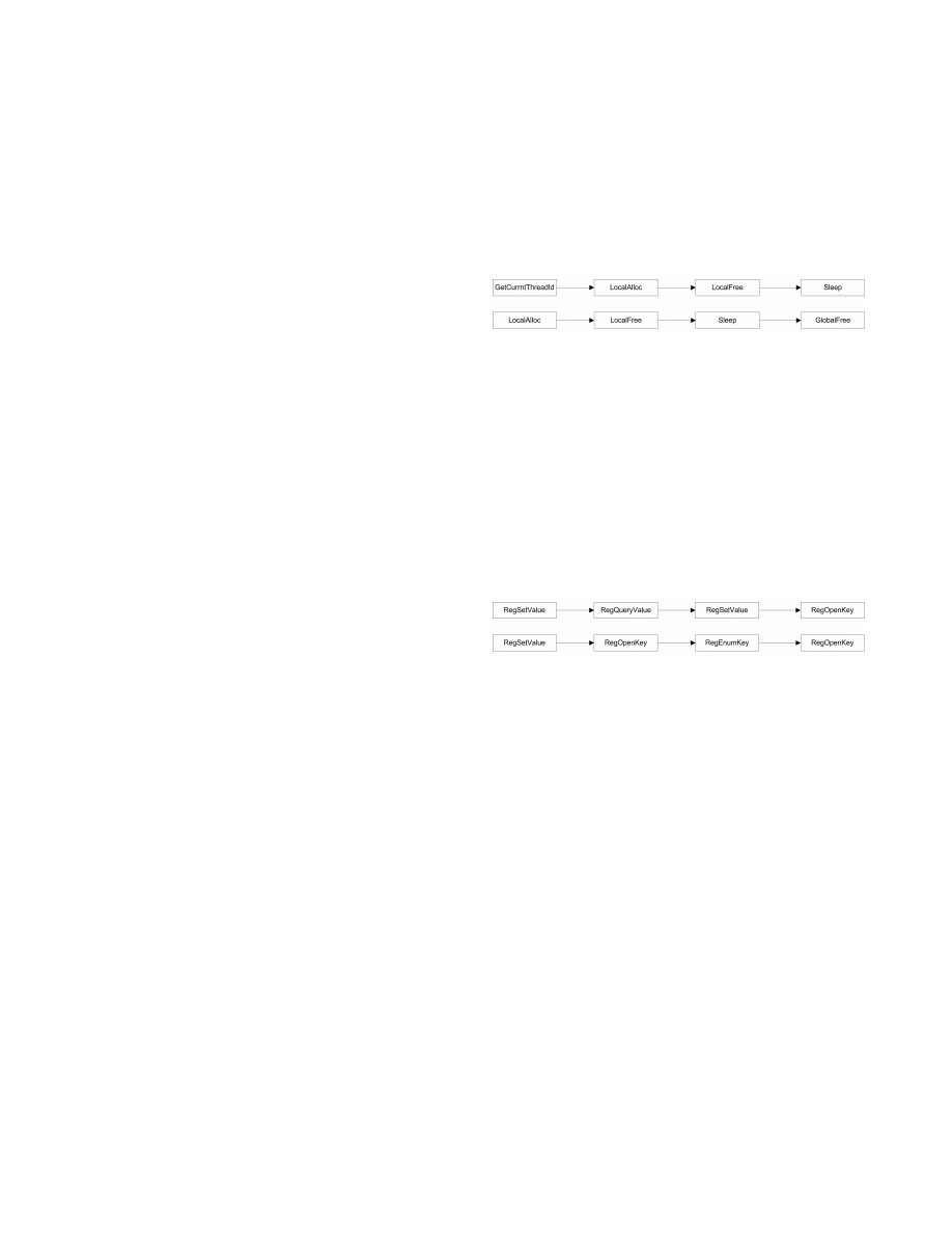
example, Table 2 and Figure 2 contain two sequences which
occur frequently in API call traces of benign programs and
are absent from API call traces of malware software. These
API calls are related to the memory management function-
ality. We have observed that benign programs – mostly for
graphics-related activities – extensively utilize memory man-
agement functionalities. Intuitively speaking, malware writ-
ers suffice on lean and mean implementations of malware
programs with low memory usage so that they can remain
unnoticed for as long as possible.

Figure 2:

API call sequences present in benign

traces and absent in malware traces

Similarly, it is shown that certain call sequences form sig-

natures of malware software. Figure 3 shows two API call
sequences which frequently occur in execution traces of mal-
ware but are absent from the traces of a benign program.
The API functions in these sequences are generally used to
access the Windows registry – a gateway to the operating
system. A malware is expected to use these API calls to ac-
cess and alter information in the registry file. Two sequences
shown in Figure 3 represent a program which first makes a
query about a registry entry and then sets it with a proper
value. The second sequence opens a registry key, retrieves
data in the key and then alters it.

Figure 3:

API call sequences present in malware

traces and absent in benign traces

Having developed an intuitive model of our data we will

now focus on the formal modeling of spatial and temporal
information.

4.

MODELING AND QUANTIFICATION OF
SPATIO-TEMPORAL INFORMATION

We have already explained in Section 3 that we can ex-

tract two types of information – spatial and temporal – from
API calls. In this section, we present formal models to sys-
tematically quantify these features. We start by presenting
a formal definition of API calls that will help in better un-
derstanding of the formal model for spatio-temporal infor-
mation.

4.1

Formal Definitions

An API call i can be formally represented by a tuple (T

i

)

of the form:

(S

i

, F

(i,1)

, F

(i,2)

, ..., F

(i,}(i))

, R

i

),

(1)

where S

i

is its identity (string name), R

i

is its return value,

and }(i) is its number of arguments. The range of }(i) in
our study is given by R(}) = {0, 1, 2, 3, 4, 5}.

The Windows operating system and third-parties provide

a large set S

T

of API calls.

Each call is represented by

Table 2: Examples of information extracted from API calls

Benign

Malware

Information

Installations

Network Utilities

Misc.

Trojans

Viruses

Worms

LocalAllocuBytesMean

48.80

18.33

59.72

95.95

111.02

100.41

GlobalFreehMemVar

261.08

298.77

274.56

58.13

49.63

51.46

Seq−1

33.33

66.67

47.83

0.00

0.00

0.00

Seq−2

33.33

66.67

44.93

0.00

0.00

0.00

a unique string S

i

∈ S

T

. In our study, we only consider

a core-functionality subset S ⊂ S

T

.

S is further divided

into seven functional subsets: (1) socket S

sock

, (2) mem-

ory management S

mm

, (3) processes and threads S

proc

, (4)

file I/O S

io

, (5) dynamic linked libraries S

dll

, (6) registry

S

reg

, and (7) network management S

nm

.

That is, S ⊇

(S

sock

S

S

mm

S

S

proc

S

S

io

S

S

dll

S

S

reg

S

S

nm

).

A trace of API calls (represented by Θ

P

) is retrieved by

executing a given program (P ). The trace length (|Θ

P

|) is an

integer variable. Θ

P

is an ordered set which is represented

as:

< T

(p,1)

, T

(p,2)

, ..., T

(p,|Θ

P

|)

>

(2)

It is important to note that executing a given program P

on different machines with different hardware and software
configurations may result in slightly different traces. In this
study, we assume that such differences, if any, are practically
negligible. We are now ready to explore the design of spa-
tial and temporal features on the basis of above-mentioned
formal representations of API calls.

4.2

Spatial Features

API calls have input arguments and return values which

can be utilized to extract useful features. Recall that the
majority of these arguments are generally address pointers
and size parameters. We now present the modeling process
of spatial information.

4.2.1

Modeling Spatial Information.

The address pointers and size parameters can be ana-

lyzed to provide a valuable insight about the memory ac-
cess patterns of an executing program. To this end, we have
handpicked arguments from a number of API calls such as
CreateThread, GetFileSize, SetFilePointer, etc. The se-
lected fields of API call arguments, depending on the cat-
egory of API call, can reflect the behavior of a program
in terms of network communication (S

sock

), memory access

(S

mm

), process/thread execution (S

proc

) and file I/O (S

io

).

We now choose appropriate measures to quantify the se-
lected spatial information.

4.2.2

Quantification.

We use fundamental statistical and information theoretic

measures to quantify the spatial information. These mea-
sures include mean (µ), variance (σ

2

), entropy (H), mini-

mum (min), and maximum (max) of given values. Mathe-
matically, for F

(i,j)

∈ ∆

F

(i,j)

, we define the statistical prop-

erties mentioned above for j

th

argument of an i

th

API call

as:

µ = E{F

(i,j)

} =

X

a

k

∈∆

F(i,j)

a

k

. Pr{F

(i,j)

= a

k

}

σ

2

= var{F

(i,j)

} =

X

a

k

∈∆

F(i,j)

(a

k

−E{F

(i,j)

})

2

.Pr{F

(i,j)

= a

k

}

H{F

(i,j)

} = −

X

a

k

∈∆

F(i,j)

a

k

log

2

(a

k

)

min{F

(i,j)

} = a

∗
k

| a

∗
k

≤ a

k

, ∀ a

k

∈ ∆

F

(i,j)

max{F

(i,j)

} = a

∗
k

| a

∗
k

≥ a

k

, ∀ a

k

∈ ∆

F

(i,j)

4.3

Temporal Features

Given a trace (represented by Θ

P

) for the program P , we

can treat every call S

i

as an element of S

p

= < S

0

, S

1

, ...,

S

|Θ

P

|

>, where S

p

represents a sequence of API calls. With-

out the loss of generality, we can also treat every consec-
utive n calls in S

p

as an element. For example, if S

p

=

< a, b, c, d, e >, and we consider two consecutive calls as an
element (n = 2), we get the sequence as < ab, bc, cd, de >.
This up-scaling also increases the dimensionality of the dis-
tribution from k to k

n

. This process not only increases the

underlying information but may also result in sparse dis-
tributions because of lack of training data. Therefore, an
inherent tradeoff exists between the amount of information,
characterized by entropy, and the minimum training data
required to build a model. Consequently, selecting appro-
priate value of n is not a trivial task and several techniques
are proposed to determine its appropriate value.

It is important to note that the up-scaled sequence with

n = 2 is in fact a simple joint distribution of two sequences
with n = 1, and so on. The joint distribution may contain
some redundant information which is relevant for a given
problem. Therefore, we need to remove the redundancy for
accurate analysis. To this end, we have analyzed a number
of statistical properties of the call sequences.

A relevant

property that has provided us interesting insights into the
statistical characteristics of call sequences is the correlation
in call sequences [13].

4.3.1

Correlation in Call Sequences.

Autocorrelation is an important statistic for determining

the order of a sequence of states. Autocorrelation describes
the correlation between the random variables in a stochastic
process at different points in time or space. For a given lag
t, the autocorrelation function of a stochastic process, X

m

(where m is the time/space index), is defined as:

ρ[t] =

E{X

0

X

t

} − E{X

0

}E{X

t

}

σ

X

0

σ

X

t

,

(3)

where E{.} represents the expectation operation and σ

X

m

is the standard deviation of the random variable at time/space

0

1

2

3

4

5

6

7

8

9

0

0.2

0.4

0.6

0.8

1

Lag

Sample Autocorrelation

(a) Matlab

0

1

2

3

4

5

6

7

8

9

0

0.2

0.4

0.6

0.8

1

Lag

Sample Autocorrelation

(b)
Trojan.Win32.Aimbot-
ee

0

1

2

3

4

5

6

7

8

9

0

0.2

0.4

0.6

0.8

1

Lag

Sample Autocorrelation

(c)
Virus.Win32.Flechal

0

1

2

3

4

5

6

7

8

9

0

0.2

0.4

0.6

0.8

1

Lag

Sample Autocorrelation

(d) Worm.Win32.ZwQQ.a

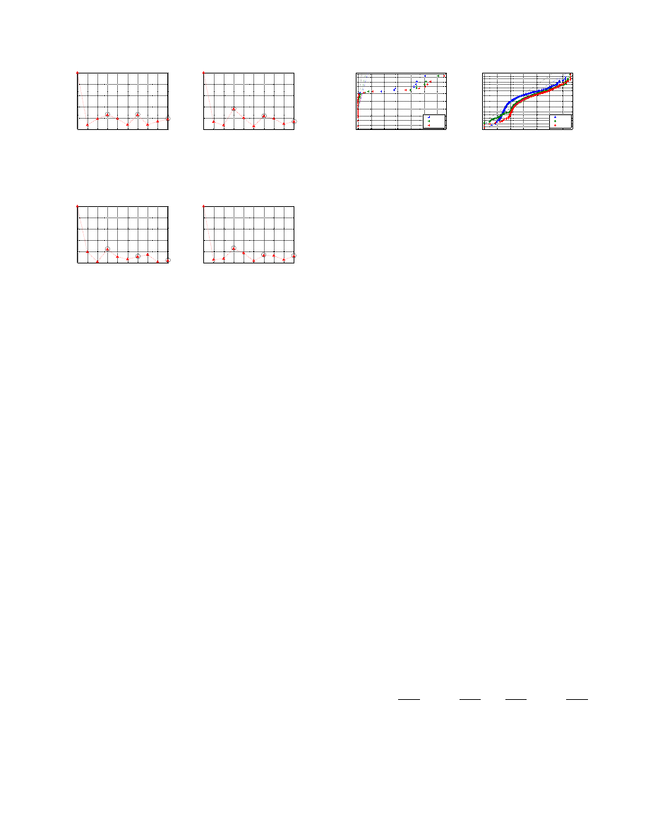
Figure 4: Sample autocorrelation functions of API
call sequences show peaks at n = 3, 6, and 9 for be-
nign, trojan, virus, and worm executables.

lag m. The value of the autocorrelation function lies in the
range [−1, 1], where ρ[t] = 1 means perfect correlation at lag
t (which is obviously true for n = 0), and ρ[t] = 0 means no
correlation at all at lag t.

To observe the dependence level in call sequences S

p

, we

calculate sample autocorrelation functions for benign and
malware programs. Figure 4 shows the sample autocorrela-
tion functions plotted versus the lag. It is evident that call
sequences show a 3

rd

order dependence because the autocor-

relation shows peaks at n = 3, 6, 9, ... in most of the cases.
This fact will be useful as we develop our statistical model
of call sequences.

4.3.2

Statistical Model of Call Sequences.

We can model API call sequence using a discrete time

Markov chain [7]. Note that the Markov chain represents
the conditional distribution. The use of conditional distri-
bution, instead of joint distribution, reduces the size of the
underlying sample space which, for the present problem, cor-
responds to removing the redundant information from the
joint distribution.

The order of a Markov chain represents the extent to

which past states determine the present state, i.e., how many
lags should be examined when analyzing higher orders. The
correlation analysis is very useful for analyzing the order of a
Markov chain process. The rationale behind this argument
is that if we take into account the past states, it should re-
duce the surprise or the uncertainty in the present state [7].
The correlation results highlight the 3

rd

order dependence in

call sequences; therefore, we use a 3

rd

order Markov chain.

Markov chain used to model the conditional distribution

has k states, where k = |S|. The probabilities of transitions
between these states are detailed in state transition matrix
T . An intuitive method to present T is to couple consecu-

0

0.1

0.2

0.3

0.4

0.5

0.6

0.01

0.02

0.05

0.10

0.25

0.50

0.75

0.90

0.95

0.98

0.99

IG

Probability

Trojan
Virus
Worm

(a) Spatial features

0

0.05

0.1

0.15

0.2

0.25

0.3

0.001

0.003

0.01

0.02

0.05

0.10

0.25

0.50

0.75

0.90

0.95

0.98

0.99

0.997

0.999

IG

Probability

Trojan
Virus
Worm

(b) Temporal features

Figure 5:

Normal probability distribution plot of

Information Gain (IG) for spatial and temporal fea-
tures

tive states together; as a result, we represent the 3

rd

order

Markov chain in the form of the state transition matrix T .

T =

2
6

6

6

6

6

6

6

6

6

6

4

t

(0,0),(0,0)

t

(0,0),(0,1)

. . .

t

(0,0),(k,k)

t

(0,1),(0,0)

t

(0,1),(0,1)

. . .

t

(0,1),(k,k)

.

.

.

.

.

.

. .

.

.

.

.

t

(0,k),(0,0)

t

(0,k),(0,1)

. . .

t

(0,k),(k,k)

t

(1,k),(0,0)

t

(1,k),(0,1)

. . .

t

(1,k),(k,k)

.

.

.

.

.

.

. .

.

.

.

.

t

(k,k),(0,0)

t

(k,k),(0,1)

. . .

t

(k,k),(k,k)

3
7

7

7

7

7

7

7

7

7

7

5

In the following text, we explore the possibility of using

probabilities in transition matrix T to quantify temporal
features of API calls.

4.3.3

Quantification.

We consider each transition probability a potential fea-

ture. However, in the transition matrix we have k

n

distinct

transition probabilities. To select the most discriminative
features, we use a feature selection procedure. To this end,
we populate two training Markov chains each from a few
benign and malware traces. Several information-theoretic
measures are proposed in the literature to evaluate the dis-
criminative quality of attributes, such as information gain
(IG ∈ [0, 1]). Information gain measures the reduction in
uncertainty if the values of an attribute are known [7]. For a
given attribute X and a class attribute Y ∈ {Benign, Malware},
the uncertainty is given by their respective entropies H(X)
and H(Y ). Then the information gain of X with respect to
Y is given by IG(Y ; X):

IG(Y ; X) = H(Y ) − H(Y |X)

We compute information gain for each element of T . For a

given element, with a counts in the benign training matrix
and b counts in the malware training matrix, IG can be
computed by [10]:

IG(a, b) = −

a

a + b

. log

2

a

a + b

−

b

a + b

. log

2

b

a + b

Finally, all potential features are sorted based on their re-

spective IG values to an ordered set T

IG

. We select T

IG

Γ

⊂

T

IG

as the final boolean feature set containing Γ transitions

with top values of IG. For this study we have used Γ = 500.

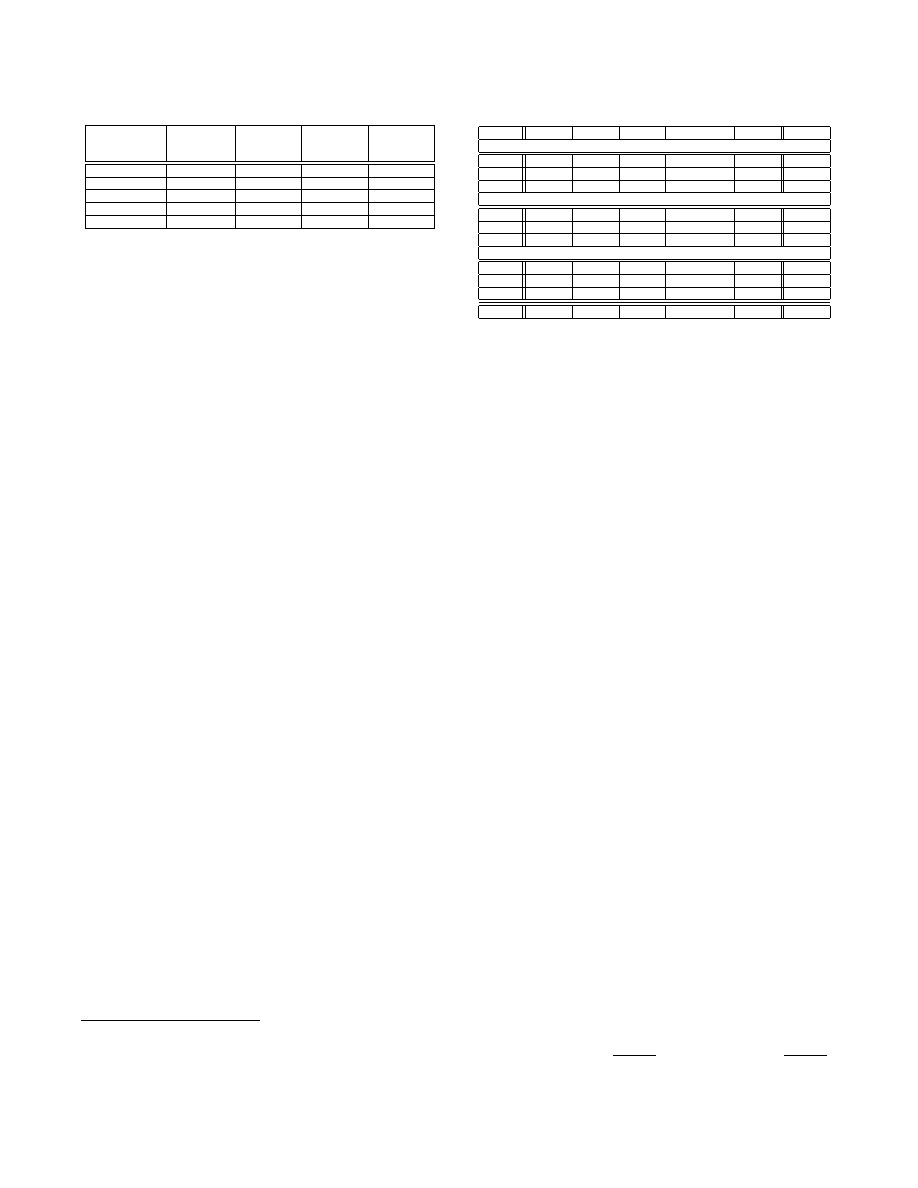
Table 3: Statistics of executable files used in this
study

Executable

Quantity

Avg.

Min.

Max.

(Type)

File Size

File Size

File Size

(KB)

(KB)

(KB)

Benign

100

1, 263

4

104, 588

Trojan

117

270

1

9, 277

Virus

165

234

4

5, 832

Worm

134

176

3

1, 301

Total

516

50

2

1, 332

4.4

Discussion

We have discussed the formal foundation of our spatio-

temporal features’ set extracted from the traces of API calls.
To analyze the classification potential of these features, we
use definition of information gain (IG). The values of IG
approaching one represent features with a higher classifica-
tion potential and vice-versa.

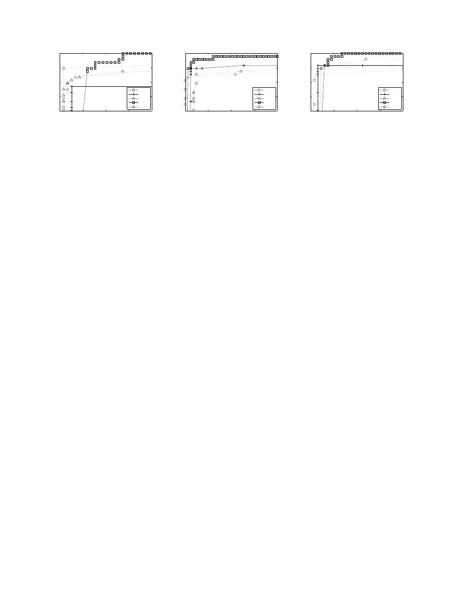
Figure 5 shows the normal probability plot of IG of spa-

tial and temporal features for trojans, viruses and worms.
It is interesting to see in Figure 5 the ‘skewed’ nature of the
IG distribution of spatial features. The majority of spatial
features have very low values of IG, but some of them also
have IG values as high as 0.7. The high IG features can
prove valuable in achieving high accuracy. In comparison,
the IG distribution of temporal features is fairly regular with
most of the IG values lie in the range of [0.0,0.4]. Another
important observation is that the means of IG distribution
of spatial features are 0.10, 0.09 and 0.08 for worms, viruses
and trojans respectively. Similarly, the means of IG dis-
tribution of temporal features are 0.16, 0.14 and 0.12 for
worms, viruses and trojans respectively. Intuitively speak-
ing – on the basis of IG values – we expect that trojans will
be most difficult to classify, followed by viruses and worms
respectively.

5.

CLASSIFICATION RESULTS AND DIS-
CUSSIONS

In this section, we explain the experiments undertaken to

evaluate the classification accuracy of our spatio-temporal
malware detection scheme. We have designed two sets of
experiments to evaluate the performance of different com-
ponents of our technique in a systematic manner. In the
first set of experiments (Experiment-1), we investigate the
merit of using spatio-temporal features’ set over standalone
spatial or temporal features’ set. We take the accuracy from
(Experiment-1) as a benchmark and then in the second set
of experiments (Experiment-2) we carry out a scalability
analysis to identify a minimal subset of API categories that
has the potential to deliver the same accuracy. In both sets
of experiments, we use the optimal configurations of differ-
ent classification algorithms

2

to achieve the best ROC (Re-

ceiver Operating Characteristics) curve for them. We first
provide a brief description of our dataset and then discuss
the accuracy results.

2

In this paper, we have used instance based learner (IBk),

decision tree (J48), Na¨ıve Bayes (NB), inductive rule learner
(RIPPER), and support vector machine (SMO) machine
learning classification algorithms [18].

Table 4: Detection accuracy for spatial (S), tempo-
ral (T) and combined (S&T) features

Alg.

IBk

J48

NB

RIPPER

SMO

Avg.

Trojan

S

0.926

0.910

0.777

0.871

0.760

0.849

T

0.958

0.903

0.945

0.932

0.970

0.942

S&T

0.963

0.908

0.966

0.959

0.970

0.953

Virus

S

0.915

0.940

0.859

0.949

0.915

0.916

T

0.937

0.956

0.974

0.945

0.971

0.957

S&T

0.954

0.963

0.990

0.954

0.968

0.966

Worm

S

0.973

0.961

0.946

0.963

0.806

0.930

T

0.942

0.968

0.962

0.953

0.963

0.958

S&T

0.958

0.966

0.984

0.975

0.963

0.969

Avg.

0.963

0.947

0.980

0.963

0.968

0.963

5.1

Dataset

The dataset used in this study consists of 416 malware and

100 benign executables. All of them are in Win32 portable
executable format.

The benign executables are obtained

from a freshly installed copy of Windows XP and applica-
tion installers. The malware executables are obtained from
a publicly available database called ‘VX Heavens Virus Col-
lection’ [3]. Table 3 provides the basic statistics of the exe-
cutables used in our study. These statistics show the diver-
sity of the executables in terms of their file sizes. We have
logged the API call traces of these files by executing them
on a freshly installed Windows XP. The logging process is
carried out using a commercial API call tracer [1]. The API
call logs obtained for this study are publicly available at
http://www.nexginrc.org/.

5.2

Experimental Setup

We now explain the experimental setup used in our study.

We have combined the benign executable trace with each
type of the malware to create three separate datasets –
benign-trojan, benign-virus and benign-worm. A stratified
10-fold cross validation procedure is followed for all experi-
ments reported later in this section. In this procedure, we
partition each dataset into 10 folds where 9 of them are used
for training and the left over fold is used for testing. This
process is repeated for all folds and the reported results are
an average of all folds.

For two-class problems, such as malware detection, the

classification decision of an algorithm may fall into one of the
four categories: (1) True Positive (TP) – correct classifica-
tion of a malicious executable as malicious, (2) True Neg-
ative (TN) – correct classification of a benign executable
as benign, (3) False Positive (FP) – wrong classification
of a benign executable as malicious, and (4) False Nega-
tive (FN) – wrong classification of a malicious executable
as benign.

We have carried out the standard ROC analysis to eval-

uate the accuracy of our system. ROC curves are exten-
sively used in machine learning and data mining to depict
the tradeoff between the true positive rate and the false pos-
itive rate of a given classifier. We quantify the accuracy (or
detection accuracy) of each algorithm by using the area un-
der ROC curve (0 ≤ AUC ≤ 1). The high values of AUCs
reflect high tp rate (=

T P

T P +F N

) and low fp rate (=

F P

F P +T N

)

[8]. At AUC = 1, tp rate = 1 and fp rate = 0.

Table 5: Detection accuracy results with different
feature sets (spatio-temporal) for all malware types
used in this study.

Alg.

IBk

J48

NB

RIPPER

SMO

Avg.

S

sock

0.524

0.479

0.513

0.520

0.513

0.510

S

mm

0.966

0.946

0.952

0.942

0.926

0.946

S

proc

0.901

0.912

0.944

0.934

0.938

0.926

S

io

0.809

0.782

0.841

0.823

0.839

0.819

S

dll

0.804

0.713

0.790

0.724

0.743

0.755

S

reg

0.962

0.922

0.923

0.929

0.937

0.935

S

nm

0.500

0.480

0.501

0.499

0.521

0.500

S

mm

S

S

io

0.975

0.950

0.986

0.956

0.963

0.966

S

mm

S

S

reg

0.962

0.951

0.950

0.953

0.926

0.948

S

io

S

S

reg

0.810

0.773

0.867

0.798

0.840

0.818

S

proc

S

S

io

0.973

0.924

0.988

0.941

0.961

0.957

S

proc

S

S

reg

0.905

0.919

0.946

0.916

0.937

0.924

S

mm

S

S

proc

0.939

0.948

0.953

0.951

0.956

0.949

5.3

Experiment-1

In the first set of experiments, we evaluate the accuracy

of spatial and temporal features separately as well as their
combination for detecting trojans, viruses and worms. The
detection accuracy results from Experiment-1 are tabu-
lated in Table 4. The bold values highlight the best accuracy
results for a particular classifier and the malware type.

It is interesting to note in Table 4 that spatial and tem-

poral features alone can provide on the average detection
accuracies of approximately 0.898 and 0.952 respectively.
However, the combined spatio-temporal features’ set provide
an average detection accuracy of 0.963 – approximately 5%
improvement over standalone features’ set.

It is interesting to see that the difference in the relative

detection accuracies of all classification algorithms is on the
average 4−5%. The last row of Table 4 provides the average
of best results obtained for all malware types with each clas-
sification algorithm. NB with spatio-temporal features’ set
provides the best detection accuracy of 0.980. It is closely
followed by SMO which provides the detection accuracy of
0.968. On the other hand, J48 provides the lowest accuracy
of 0.947. Another important observation is that once we use
the combined spatio-temporal features, the classification ac-
curacies of NB for trojan and virus categories significantly
improves to 0.966 and 0.990 respectively.

An analysis of Table 4 highlights the relative difficulty

of detecting trojans, viruses and worms.

The lowest de-

tection accuracy is obtained for trojans because trojans are
inherently designed to appear similar to benign programs.
Worms are the easiest to detect while viruses stand in be-
tween. Note that this empirical outcome is consistent with
our prediction in Section 4.4 based on the IG values of the
extracted features for these malware types.

We also show ROC plots in Figure 6 for detection accuracy

of different types of malware for all classification algorithms
by using spatio-temporal features. The plots further vali-
date that the tp rate of NB quickly converges to its highest
values. The ROC plots also confirm that trojans are the
most difficult to detect while it is relatively easier to detect
worms.

5.4

Experiment-2

The processing and memory overheads of monitoring run-

time API calls and storing their traces might lead to sig-

nificant performance bottlenecks. Therefore, we have also
performed a scalability analysis to quantify the contribution
of different functional categories of API calls towards the
detection accuracy. By using this analysis, we can identify
redundant API categories; as a result, we can find the min-
imal subset of API categories that provide the same detec-
tion accuracy as in Experiment-1. This analysis can help
in improving the efficiency and performance of our proposed
scheme.

We have performed this analysis in a systematic manner.

First we evaluate the detection accuracy of individual API
categories namely S

sock

, S

mm

, S

proc

, S

io

, S

dll

, S

reg

, and S

nm

.

The results of our scalability experiments are tabulated in
Table 5. We can conclude from Table 5 that the detection
accuracies of S

mm

, S

reg

, S

proc

, and S

io

is very promising. We

have tried all possible combinations (

4

C

2

= 6) of the promis-

ing functional categories. The results of our experiments
show that S

mm

S

S

io

provides the best detection accuracy

of 0.966. We have also tried higher-order combinations of
API categories but the results do not improve significantly.

6.

CONCLUSION AND FUTURE WORK

In this paper, we have presented our run-time malware

analysis and detection scheme that leverages spatio-temporal
information available in API calls. We have proven our the-
sis that combined spatio-temporal features’ set increases the
detection accuracy than standalone spatial or temporal fea-
tures’ set. Moreover, our scalability analysis shows that our
system achieves the detection accuracy of 0.97 by only mon-
itoring API calls from memory management and file I/O
categories.

It is important to emphasize that spatial and temporal

features use completely different data models; therefore, in-
tuitively speaking they have the potential to provide an ex-
tra layer of robustness to evasion attempts. For example, if
a crafty attacker manipulates the sequence of system calls
to evade temporal features, then spatial features will help to
sustain high detection accuracy and vice-versa. In future, we
want to quantify the effect of evasion attempts by a crafty
attacker on our scheme.

Acknowledgments

The research presented in this paper is supported by the
grant # ICTRDF/AN/2007/37, for the project titled AIS-
GPIDS, by the National ICT R&D Fund, Ministry of In-
formation Technology, Government of Pakistan. The infor-
mation, data, comments, and views detailed herein may not
necessarily reflect the endorsements of views of the National
ICT R&D Fund.

7.

REFERENCES

[1] API Monitor - Spy and display API calls made by

Win32 applications, available at
http://www.apimonitor.com.

[2] Overview of the Windows API, available at

http://msdn.microsoft.com/en-us/library/
aa383723(VS.85).aspx.

[3] VX Heavens Virus Collection, VX Heavens,

http://vx.netlux.org/.

[4] F. Ahmed, H. Hameed, M.Z. Shafiq, M. Farooq,

“Using Spatio-Temporal Information in API Calls with

0

0.05

0.1

0.15

0.2

0.8

0.85

0.9

0.95

1

fp rate

tp rate

IBK
J48
Ripper
NB
SMO

(a) Trojan-Benign (Zoomed)

0

0.05

0.1

0.15

0.2

0.8

0.85

0.9

0.95

1

fp rate

tp rate

IBK
J48
Ripper
NB
SMO

(b) Virus-Benign (Zoomed)

0

0.05

0.1

0.15

0.2

0.8

0.85

0.9

0.95

1

fp rate

tp rate

IBK
J48
Ripper
NB
SMO

(c) Worm-Benign (Zoomed)

Figure 6: ROC plots for detecting malicious executables using spatial and temporal features.

Machine Learning Algorithms for Malware Detection
and Analysis”, Technical Report,
TR-nexGINRC-2009-42, 2009, available at
http://www.nexginrc.org/papers/tr42-faraz.pdf

[5] P. Beaucamps J.-Y. Marion, “Optimized control flow

graph construction for malware detection”,
International Workshop on the Theory of Computer
Viruses (TCV), France, 2008.

[6] M. Christodorescu, S. Jha, S.A. Seshia, D. Song, R.E.

Bryant, “Semantics-Aware Malware Detection”, IEEE
Symposium on Security and Privacy (S&P), IEEE
Press, USA, 2005.

[7] T.M. Cover, J.A. Thomas, “Elements of Information

Theory”, Wiley-Interscience, 1991.

[8] T. Fawcett, “ROC Graphs: Notes and Practical

Considerations for Researchers”, Techincal Report, HP
Labs, CA, 2003-4, USA, 2003.

[9] S. Forrest, S.A. Hofmeyr, A. Somayaji, T.A.

Longstaff, “A Sense of Self for Unix Processes”, IEEE
Symposium on Security and Privacy (S&P), IEEE
Press, pp. 120-128, USA, 1996

[10] J. Han, M. Kamber, “Data Mining: Concepts and

Techniques”, Morgan Kaufmann, 2000.

[11] D. Mutz, F. Valeur, C. Kruegel, G. Vigna,

“Anomalous System Call Detection”, ACM

Transactions on Information and System Security
(TISSEC), 9(1), pp. 61-93, ACM Press, 2006.

[12] C. Parampalli, R. Sekar, R. Johnson, “A Practical

Mimicry Attack Against Powerful System-Call
Monitors”, ACM Symposium on Information,
Computer and Communications Security (AsiaCCS),
pp. 156-167, Japan, 2008.

[13] M.Z. Shafiq, S.A. Khayam, M. Farooq, “Embedded

Malware Detection using Markov n-grams”, Detection
of Intrusions and Malware, and Vulnerability
Assessment (DIMVA), pp. 88-107, Springer, France,
2008.

[14] G. Tandon, P. Chan, “Learning Rules from System

Call Arguments and Sequences for Anomaly
Detection”, ICDM Workshop on Data Mining for
Computer Security (DMSEC), pp. 20-29, IEEE Press,
USA, 2003.

[15] D. Wagner, P. Soto, “Mimicry Attacks on Host-Based

Intrusion Detection Systems”, ACM Conference on
Computer and Communications Security (CCS), pp.
255-264, ACM Press, USA, 2002.

[16] C. Warrender, S. Forrest, B. Pearlmutter, “Detecting

Intrusions Using System Calls: Alternative Data
Models”, IEEE Symposium on Security and Privacy
(S&P), pp. 133-145, IEEE Press, USA, 1999.

[17] A. Wespi, M. Dacier, H. Debar, “Intrusion Detection

Using Variable-Length Audit Trail Patterns”, Recent
Advances in Intrusion Detection (RAID), pp. 110-129,
Springer, France, 2000.

[18] I.H. Witten, E. Frank, “Data mining: Practical

machine learning tools and techniques”, Morgan
Kaufmann, 2nd edition, USA, 2005.