
Advanced Mechanics

This page intentionally left blank

Advanced Mechanics
From Euler’s Determinism to Arnold’s Chaos
S. G. Rajeev
Department of Physics and Astronomy, Department of Mathematics
University of Rochester, Rochester, NY14627
3

3
Great Clarendon Street, Oxford, OX2 6DP,
United Kingdom
Oxford University Press is a department of the University of Oxford.
It furthers the University’s objective of excellence in research, scholarship,
and education by publishing worldwide. Oxford is a registered trade mark of
Oxford University Press in the UK and in certain other countries
c
S. G. Rajeev 2013
The moral rights of the author have been asserted
First Edition published in 2013
Impression: 1
All rights reserved. No part of this publication may be reproduced, stored in
a retrieval system, or transmitted, in any form or by any means, without the
prior permission in writing of Oxford University Press, or as expressly permitted
by law, by licence or under terms agreed with the appropriate reprographics
rights organization. Enquiries concerning reproduction outside the scope of the
above should be sent to the Rights Department, Oxford University Press, at the
address above
You must not circulate this work in any other form
and you must impose this same condition on any acquirer
Published in the United States of America by Oxford University Press
198 Madison Avenue, New York, NY 10016, United States of America
British Library Cataloguing in Publication Data
Data available
Library of Congress Control Number: 2013938985
ISBN 978–0–19–967085–7
ISBN 978–0–19–967086–4 (pbk.)
Printed and bound by
CPI Group (UK) Ltd, Croydon, CR0 4YY

This book is dedicated to Sarada Amma and Gangadharan Pillai, my parents.

This page intentionally left blank

Preface
Classical mechanics is the oldest and best understood part of physics. This does not mean
that it is cast in marble yet, a museum piece to be admired reverently from a distance.
Instead, mechanics continues to be an active area of research by physicists and mathemati-
cians. Every few years, we need to re-evaluate the purpose of learning mechanics and look
at old material in the light of modern developments.
The modern theories of chaos have changed the way we think of mechanics in the
last few decades. Previously formidable problems (three body problem) have become
easy to solve numerically on personal computers. Also, the success of quantum mechan-
ics and relativity gives new insights into the older theory. Examples that used to be
just curiosities (Euler’s solution of the two center problem) become starting points for
physically interesting approximation methods. Previously abstract ideas (Julia sets) can
be made accessible to everyone using computer graphics. So, there is a need to change
the way classical mechanics is taught to advanced undergraduates and beginning graduate
students.
Once you have learned basic mechanics (Newton’s laws, the solution of the Kepler
problem) and quantum mechanics (the Schr¨
odinger equation, hydrogen atom) it is time
to go back and relearn classical mechanics in greater depth. It is the intent of this book
to take you through the ancient (the original meaning of “classical”) parts of the subject
quickly: the ideas started by Euler and ending roughly with Poincar´
e. Then we take up the
developments of twentieth century physics that have largely to do with chaos and discrete
time evolution (the basis of numerical solutions).
Although some knowledge of Riemannian geometry would be helpful, what is needed
is developed here. We will try to use the minimum amount of mathematics to get as deep
into physics as possible. Computer software such as Mathematica, Sage or Maple are very
useful to work out examples, although this book is not about computational methods.
Along the way you will learn about: elliptic functions and their connection to the
arithmetic-geometric-mean; Einstein’s calculation of the perihelion shift of Mercury; that
spin is really a classical phenomenon; how Hamilton came very close to guessing wave
mechanics when he developed a unified theory of optics and mechanics; that Riemannian
geometry is useful to understand the impossibility of long range weather prediction; why
the maximum of the potential is a stable point of equilibrium in certain situations; the
similarity of the orbits of particles in atomic traps and of the Trojan asteroids.
By the end you should be ready to absorb modern research in mechanics, as well as
ready to learn modern physics in depth.
The more difficult sections and problems that you can skip on a first reading are marked
with asterisks. The more stars, the harder the material. I have even included some problems
whose answers I do not know, as research projects.
Mechanics is still evolving. In the coming years we will see even more complex problems
solved numerically. New ideas such as renormalization will lead to deeper theories of chaos.
Symbolic computation will become more powerful and change our very definition of what

viii
Preface
constitutes an analytic solution of a mechanical problem. Non-commutative geometry could
become as central to quantum mechanics as Riemannian geometry is to classical mechanics.
The distinction between a book and a computer will disappear, allowing us to combine text
with simulations. A mid-twenty-first century course on mechanics will have many of the
ingredients in this book, but the emphasis will be different.

Acknowledgements
My teacher, A. P. Balachandran, as well as my own students, formed my view of mechanics.
This work is made possible by the continued encouragement and tolerance of my wife. I also
thank my departmental colleagues for allowing me to pursue various directions of research
that must appear esoteric to them.
For their advice and help I thank Sonke Adlung and Jessica White at Oxford University
Press, Gandhimathi Ganesan at Integra, and the copyeditor Paul Beverley. It really does
take a village to create a book.

This page intentionally left blank

Contents
The Variational principle of mechanics
Deduction from quantum mechanics
The orbit of a planet lies on a plane which contains the Sun
The line connecting the planet to the Sun sweeps equal areas
in equal times
Planets move along elliptical orbits with the Sun at a focus
The ratio of the cube of the semi-major axis to the square
of the period is the same for all planets

xii
Contents
Infinitesimal canonical transformations
Symmetries and conservation laws
Hamiltonian formulation of geodesics
Geodesic formulation of Newtonian mechanics
Geodesics in general relativity
The classical limit of the Schr¨
Hamilton–Jacobi equation in Riemannian manifolds
10.1 The simple harmonic oscillator
10.2 The general one-dimensional system
10.3 Bohr–Sommerfeld quantization
10.5 The relativistic Kepler problem
10.6 Several degrees of freedom
11.5 Montgomery’s pair of pants
12 The restricted three body problem

Contents
xiii
12.6 The second derivative of the potential
14 Poisson and symplectic manifolds
14.1 Poisson brackets on the sphere
15.1 First order symplectic integrators
15.2 Second order symplectic integrator
15.3 Chaos with one degree of freedom
16 Dynamics in one real variable
17 Dynamics on the complex plane
17.3 Dynamics of a Mobius transformation
18.2 Diagonalization of matrices
18.3 Normal form of circle maps

This page intentionally left blank

2.1
The catenoid.
10
3.1
Elliptic curves.
15
4.1
The potential of the Kepler problem.
24
6.1
Orbits of the damped harmonic oscillator.
34
6.2
The stereographic co-ordinate on the sphere.
36
6.3
The Lorenz system.
41
12.1 Hill’s regions for ν = 0.2. The orbit cannot enter the gray region, which
shrinks as H grows.
99
15.1 Symplectic integration of the pendulum.
119
15.2 Non-symplectic integration of the pendulum.
119
15.3 The Chirikov standard map for the initial point p = 0.1, q = 1 and
various values of K.
122
16.1 The cobweb diagram of f (x) = 2.9x(1
− x) with initial point x
0
= 0.2.
129
16.2 The cobweb diagram of f (x) = 3.1x(1
− x) showing a cycle of period 2.
131
16.3 The cobweb diagram of f (x) = 3.4495x(1
− x) showing a cycle of period 4.
133
16.4 The cycles of the map f (x) = μ sin(πx) for the range 0 < μ < 1.
135
17.1 Julia sets for z
2
+ c for various values of c.
146
17.2 More Julia sets.
146
17.3 Orbits of a hyperbolic Mobius transformation.
147
17.4 The Mandelbrot set.
147

This page intentionally left blank

Many problems in physics involve finding the minima (more generally extrema) of functions.
For example, the equilibrium positions of a static system are the extrema of its potential
energy; stable equilibria correspond to local minima. It is a surprise that even dynamical
systems, whose positions depend on time, can be understood in terms of extremizing a
quantity that depends on the paths: the action. In fact, all the fundamental physical laws
of classical physics follow from such variational principles. There is even a generalization to
quantum mechanics, based on averaging over paths where the paths of extremal action make
the largest contribution. In essence, the calculus of variations is the differential calculus of
functions that depend on an infinite number of variables. For example, suppose we want
to find the shortest curve connecting two different points on the plane. Such a curve can
be thought of as a function (x(t), y(t)) of some parameter (like time). It must satisfy the
boundary conditions
x(t
1
) = x
1
, y(t
1
) = y
1
x(t
2
) = x
2
, y(t
2
) = y
2
where the initial and final points are given. The length is
S[x, y] =
t
2
t
1
˙x
2
+ ˙
y
2
dt
This is a function of an infinite number of points because we can make some small
changes δx(t), δy(t) at each time t independently. We can define a differential, the
infinitesimal change of the length under such a change:
δS =
t
2
t
1
˙xδ ˙x + ˙
yδ ˙
y
˙x
2
+ ˙
y
2
dt
Generalizing the idea from the calculus of several variables, we expect that at the ex-
tremum, this quantity will vanish for any δx, δy. This condition leads to a differential
equation whose solution turns out to be (no surprise) a straight line. There are two key
ideas here. First of all, the variation of the time derivative is the time derivative of the
variation:
δ ˙x =
d
dt
δx

2
The variational principle
This is essentially a postulate on the nature of the variation. (It can be further justified
if you want.) The second idea is an integration by parts, remembering that the variation
must vanish at the boundary (we are not changing the initial and final points).
δx(t
1
) = δx(t
2
) = 0 = δy(t
1
) = δy(t
2
)
Now,
˙x
˙x
2
+ ˙
y
2
d
dt
δx =
d
dt
˙x
˙x
2
+ ˙
y
2
δx
−
d
dt
˙x
˙x
2
+ ˙
y
2
δx
and similarly with δy. Then
δS =
t
2
t
1
d
dt
˙x
˙x
2
+ ˙
y
2
δx +
˙
y
˙x
2
+ ˙
y
2
δy
dt
−
t
2
t
1
d
dt
˙x
˙x
2
+ ˙
y
2
δx +
d
dt
˙
y
˙x
2
+ ˙
y
2
δy
dt
The first term is a total derivative and becomes
˙x
˙x
2
+ ˙
y
2
δx +
˙
y
˙x
2
+ ˙
y
2
δy
t
2
t
1
= 0
because δx and δy both vanish at the boundary. Thus
δS =
−
t
2
t
1
d
dt
˙x
˙x
2
+ ˙
y
2
δx +
d
dt
˙
y
˙x
2
+ ˙
y
2
δy
dt
In order for this to vanish for any variation, we must have
d
dt
˙x
˙x
2
+ ˙
y
2
= 0 =
d
dt
˙
y
˙x
2
+ ˙
y
2
That is because we can choose a variation that is only non-zero in some tiny (as small you
want) neighborhood of a particular value of t. Then the quantity multiplying it must vanish,
independently at each value of t. These differential equations simply say that the vector
( ˙x, ˙
y) has constant direction: (
˙x
√
˙x
2
+ ˙y
2
,
˙y
√
˙x
2
+ ˙y
2
) is just the unit vector along the tangent.
So the solution is a straight line. Why did we do all this work to prove an intuitively obvious
fact? Because sometimes intuitively obvious facts are wrong. Also, this method generalizes
to situations where the answer is not at all obvious: what is the curve of shortest length
between two points that lie entirely on the surface of a sphere?

Euler–Lagrange equations
3
In many problems, we will have to find the extremum of a quantity
S[q] =
t
2
t
1
L[q, ˙
q, t]dt
where q
i
(t) are a set of functions of some parameter t. We will call them position and time
respectively, although the actual physical meaning may be something else in a particular
case. The quantity S[q], whose extremum we want to find, is called the action. It depends
on an infinite number of independent variables, the values of q at various times t. It is
the integral of a function (called the Lagrangian) of position and velocity at a given time,
integrated on some interval. It can also depend explicitly on time; if it does not, there are
some special tricks we can use to simplify the solution of the problem.
As before, we note that at an extremum S must be unchanged under small variations
of q. Also we assume the identity
δ ˙
q
i
=
d
dt
δq
i
We can now see that
δS =
t
2
t
1
i
δ ˙
q
i
∂L
∂ ˙
q
i
+ δq
i
∂L
∂q
i
dt
=
t
2
t
1
i
dδq
i
dt
∂L
∂ ˙
q
i
+ δq
i
∂L
∂q
i
dt
We then do an integration by parts:
=
t
2
t
1
i
d
dt
δq
i
∂L
∂ ˙
q
i
dt
+
t
2
t
1
i
−
d
dt
∂L
∂ ˙
q
i
+
∂L
∂q
i
δq
i
dt
Again in physical applications, the boundary values of q at times t
1
and t
2
are given. So
δq
i
(t
1
) = 0 = δq
i
(t
2
)
Thus
t
2
t
1
i
d
dt
δq
i
∂L
∂ ˙
q
i
dt =
δq
i
∂L
∂ ˙
q
i
t
2
t
1
= 0
and at an extremum,

4
The variational principle
t
2
t
1
i
−
d
dt
∂L
∂ ˙
q
i
+
∂L
∂q
i
δq
i
dt = 0
Since these have to be true for all variations, we get the differential equations
−
d
dt
∂L
∂ ˙
q
i
+
∂L
∂q
i
= 0
This ancient argument is due to Euler and Lagrange, of the pioneering generation that
figured out the consequences of Newton’s laws. The calculation we did earlier is a special
case. As an exercise, re-derive the equations for minimizing the length of a curve using the
Euler–Lagrange equations.
The Variational principle of mechanics
Newton’s equation of motion of a particle of mass m and position q moving on the line,
under a potential V (q), is
m¨
q =
−
∂V
∂q
There is a quantity L(q, ˙
q) such that the Euler–Lagrange equation for minimizing S =
L[q, ˙
q]dt is just this equation.
We can write this equation as
d
dt
[m ˙
q] +
∂V
∂q
= 0
So if we had
m ˙
q =
∂L
∂ ˙
q
,
∂L
∂q
=
−
∂V
∂q
we would have the right equations. One choice is
L =
1
2
m ˙
q
2
− V (q)
This quantity is called the Lagrangian. Note that it is the difference of kinetic and
potential energies, and not the sum. More generally, the coordinate q may be replaced by a
collection of numbers q
i
, i = 1,
· · · , n which together describe the instantaneous position of
a system of particles. The number n of such variables needed is called the number of degrees
of freedom. Part of the advantage of the Lagrangian formalism over the older Newtonian
one is that it allows even curvilinear co-ordinates: all you have to know are the kinetic
energy and potential energy in these co-ordinates. To be fair, the Newtonian formalism is
more general in another direction, as it allows forces that are not conservative (a system
can lose energy).

Deduction from quantum mechanics
∗
5
Example 1.1: The kinetic energy of a particle in spherical polar co-ordinates is
1
2
m
˙r
2
+ r
2
˙
θ
2
+ r
2
sin
2
θ ˙
φ
2
Thus the Lagrangian of the Kepler problem is
L =
1
2
m
˙r
2
+ r
2
˙
θ
2
+ r
2
sin
2
θ ˙
φ
2
+
GM m
r
Deduction from quantum mechanics
Classical mechanics is the approximation to quantum mechanics, valid when the action
is small compared to Planck’s constant
∼ 6 × 10
−34
m
2
kg s
−1
. So we should be able
to deduce the variational principle of classical mechanics as the limit of some principle
of quantum mechanics. Feynman’s action principle of quantum mechanics says that the
probability amplitude for a system to start at q
1
at time t
1
and end at q
2
at time t
2
is
K(q
, q
|t) =
q
(t
2
)=q
2
q
(t
1
)=q
1
e
i
S
[q]
Dq
This is an infinite dimensional integral over all paths (functions of time) that satisfy these
boundary conditions. Just as classical mechanics can be formulated in terms of the differen-
tial calculus in function spaces (variational calculus), quantum mechanics uses the integral
calculus in function spaces. In the limit of small
the oscillations are very much more pro-
nounced: a small change in the path will lead to a big change in the phase of the integrand,
as the action is divided by
. In most regions of the domain of integration, the integral
cancels itself out: the real and imaginary parts change sign frequently. The exception is the
neighborhood of an extremum, because the phase is almost constant and so the integral
will not cancel out. This is why the extremum of the action dominates in the classical limit
→ 0. The best discussion of these ideas is still in Feynman’s classic paper Feynman (1948).
1.3.1
The definition of the path integral
Feynman’s paper might alarm readers who are used to rigorous mathematics. Much of the
work of Euler was not mathematically rigorous either: the theorems of variational calculus
are from about 1930s (Sobolev, Morse et al.), about two centuries after Euler. The theory
of the path integral is still in its infancy. The main step forward was by Wiener who
defined integrals of the sort we are using, except that instead of being oscillatory (with the
i in the exponential) they are decaying. A common trick is to evaluate the path integral
for imaginary time, where theorems are available, then analytically continue to real time
when the mathematicians aren’t looking. Developing an integral calculus in function spaces
remains a great challenge for mathematical physics of our time.
Problem 1.1: Find the solution to the Euler–Lagrange equations that minimize
S[q] =
1
2
a
0
˙
q
2
dt

6
The variational principle
subject to the boundary conditions
q(0) = q
0
,
q(a) = q
1
Problem 1.2: Show that, although the solution to the equations of a harmonic
oscillator is an extremum of the action, it need not be a minimum, even locally.
Solution
The equation of motion is
¨
q + ω
2
q = 0
which follows from the action
S[q] =
1
2
t
2
t
1
˙
q
2
− ω
2
q
2
dt
A small perturbation q
→ q + δq will not change the boundary conditions if δq,
vanish at t
1
, t
2
. It will change the action by
S[q + δq] = S[q] +
t
2
t
1
˙
qδ ˙
q
− ω
2
qδq
dt +
1
2
t
2
t
1
(δ ˙
q)
2
− ω
2
(δq)
2
dt
The second term will vanish if q satisfies the equations of motion. An example
of a function that vanishes at the boundary is
δq(t) = A sin
nπ(t
− t
1
)
t
2
− t
1
,
n
∈ Z
Calculate the integral to get
S[q + δq] = S[q] + A
2
t
2
− t
1
4
nπ
t
2
− t
1
2
− ω
2
If the time interval is long enough t
2
− t
1
>
nπ
ω
such a change will lower the
action. The longer the interval, the more such variations exist.
Problem 1.3: A steel cable is hung from its two end points with co-ordinates
(x
1
, y
1
) and (x
2
, y
2
). Choose a Cartesian co-ordinate system with the y-axis ver-
tical and the x-axis horizontal, so that y(x) gives the shape of the chain. Assume
that its weight per unit length is some constant μ. Show that the potential
energy is
μ
x
2
x
1
1 + y
2
(x)y(x)dx
Find the condition that y(x) must satisfy in order that this be a minimum. The
solution is a curve called a catenary. It also arises as the solution to some other
problems. (See next chapter.)

Recall that if q is a Cartesian co-ordinate,
p =
∂L
∂ ˙
q
is the momentum in that direction. More generally, for any co-ordinate q
i
the quantity
p
i
=
∂L
∂ ˙
q
i
is called the generalized momentum conjugate to q
i
. For example, in spherical polar co-
ordinates the momentum conjugate to φ is
p
φ
= mr
2
˙
φ
You can see that this has the physical meaning of angular momentum around the
third axis.
This definition of generalized momentum is motivated in part by a direct consequence of
it: if L happens to be independent of a particular co-ordinate q
i
(but might depend on ˙
q
i
),
then the momentum conjugate to it is independent of time, that is, it is conserved:
∂L
∂q
i
= 0 =
⇒
d
dt
∂L
∂ ˙
q
i
= 0
For example, p
φ
is a conserved quantity in the Kepler problem. This kind of information
is precious in solving a mechanics problem; so the Lagrangian formalism which identi-
fies such conserved quantities is very convenient to actually solve for the equations of a
system.

8
Conservation laws
L can have a time dependence through its dependence of q, ˙
q as well as explicitly. The total
time derivative is
dL
dt
=
i
˙
q
i
∂L
∂q
i
+
i
¨
q
i
∂L
∂ ˙
q
i
+
∂L
∂t
The E-L equations imply
d
dt
i
p
i
˙
q
i
− L
=
−
∂L
∂t
,
p
i
=
∂L
∂ ˙
q
i
In particular, if L has no explicit time dependence, the quantity called the hamiltonian,
H =
i
p
i
˙
q
i
− L
is conserved.
∂L
∂t
= 0 =
⇒
dH
dt
= 0
What is its physical meaning? Consider the example of a particle in a potential
L =
1
2
m ˙
q
2
− V (q)
Since the kinetic energy T is a quadratic function of ˙
q, and V is independent of ˙
q,
p ˙
q = ˙
q
∂T
∂ ˙
q
= 2T
Thus
H = 2T
− (T − V ) = T + V
Thus the hamiltonian, in this case, is the total energy.
More generally, if the kinetic energy is quadratic in the generalized velocities ˙
q
i
(which
is true very often) and if the potential energy is independent of velocities (also true often),
the hamiltonian is the same as energy. There are some cases where the hamiltonian and
energy are not the same though: for example, when we view a system in a reference frame
that is not inertial. But these are unusual situations.

Minimal surface of revolution
9
Although the main use of the variational calculus is in mechanics, it can also be used to
solve some interesting geometric problems. A minimal surface is a surface whose area is
unchanged under small changes of its shape. You might know that for a given volume, the
sphere has minimal area. Another interesting question in geometry is to ask for a surface
of minimal area which has a given curve (or a disconnected set of curves) as boundary.
The first such problem was solved by Euler. What is the surface of revolution of minimal
area, with given radii at the two ends? Recall that a surface of revolution is what you get
by taking some curve y(x) and rotating it around the x-axis. The cross-section at x is a
circle of radius y(x), so we assume that y(x) > 0. The boundary values y(x
1
) = y
1
and
y(x
2
) = y
2
are given. We can, without loss of generality, assume that x
2
> x
1
and y
2
> y
1
.
What is the value of the radius y(x) in between x
1
and x
2
that will minimize the area of this
surface?
The area of a thin slice between x and x + dx is 2πy(x)ds where ds =
1 + y
2
dx is the
arc length of the cross-section. Thus the quantity to be minimized is
S =
x
2
x
1
y(x)
1 + y
2
dx
This is the area divided by 2π.
We can derive the Euler–Lagrange equation as before: y is analogous to q and x is
analogous to t. But it is smarter to exploit the fact that the integrand is independent of x:
there is a conserved quantity
H = y
∂L
∂y
− L. L = y(x)
1 + y
2
That is
H = y
y
2
1 + y
2
− y
1 + y
2
H
1 + y
2
=
− y
y
=
y
2
H
2
− 1
y
y
1
dy
y
2
H
2
− 1
= x
− x
1
The substitution
y = H cosh θ
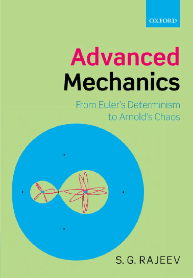
10
Conservation laws
Fig. 2.1
The catenoid.
evaluates the integral:
H[θ
− θ
1
] = x
− x
1
θ =
x
− x
1
H
+ θ
1
y = H cosh
x
− x
1
H
+ θ
1
The constants of integration are fixed by the boundary conditions
y
1
= H cosh θ
1
y
2
= H cosh
x
2
− x
1
H
+ θ
1
The curve y = H cosh
x
H
+ constant
is called a catenary; the surface you get by re-
volving it around the x-axis is the catenoid (see Fig. 2.1). If we keep the radii fixed and
move the boundaries far apart along the x-axis, at some critical distance, the surface will
cease to be of minimal area. The minimal area is given by the disconnected union of two
disks with the circles as boundaries.
Problem 2.1: The Lagrangian of the Kepler problem (Example 1.1) does not
depend on the angle. What is the conserved quantity implied by this fact?
Problem 2.2: A soap bubble is bounded by two circles of equal radii. If the
bounding circles are moved apart slowly, at some distance the bubble will break
into two flat disks. Find this critical distance in terms of the bounding radius.

Consider a mass g suspended from a fixed point by a rigid rod of length l. Also, it is only
allowed to move in a fixed vertical plane.
The angle θ from the lowest point on its orbit serves as a position co-ordinate. The
kinetic energy is
T =
1
2
ml
2
˙
θ
2
and the potential energy is
V(θ) = mgl(1
− cos θ)
Thus
T
− V = ml
2
1
2
˙
θ
2
−
g
l
(1
− cos θ)
The overall constant will not matter to the equations of motion. So we can choose as
Lagrangian
L =
1
2
˙
θ
2
−
g
l
(1
− cos θ)
This leads to the equation of motion
¨
θ +
g
l
sin θ = 0
For small angles θ
π this is the equation for a harmonic oscillator with angular frequency
ω =
g
l
But for large amplitudes of oscillation the answer is quite different. To simplify calculations
let us choose a unit of time such that, g = l; i.e., such that ω = 1. Then
L =
1
2
˙
θ
2
− (1 − cos θ)

12
The simple pendulum
We can make progress in solving this system using the conservation of energy
H =
˙
θ
2
2
+ [1
− cos θ]
The key is to understand the critical points of the potential. The potential energy has
a minimum at θ = 0 and a maximum at θ = π. The latter corresponds to an unstable equi-
librium point: the pendulum standing on its head. If the energy is less than this maximum
value
H < 2
the pendulum oscillates back and forth around its equilibrium point. At the maximum
angle, ˙
θ = 0 so that it is given by a transcendental equation
1
− cos θ
0
= H
The motion is periodic, with a period T that depends on energy. That is, we have
sin θ(t + T ) = sin θ(t)
It will be useful to use a variable which takes some simple value at the maximum deflection;
also we would like it to be a periodic function of the angle. The condition for maximum
deflection can be written
2
H
sin
θ
0
2
=
±1
This suggests that we use the variable
x =
2
H
sin
θ
2
so that, at maximum deflection, we simply have x =
±1. Define also a quantity that
parametrizes the energy
k =
H
2
,
x =
1
k
sin
θ
2
Changing variables,
˙x =
1
2k
cos
θ
2
˙
θ,
˙x
2
=
1
4k
2
1
− sin
2
θ
2
˙
θ
2
=
1
4
1
k
2
− x
2
˙
θ
2

Primer on Jacobi functions
13
Conservation of energy becomes
2k
2
= 2
˙x
2
k
−2
− x
2
+ 2k
2
x
2
Thus we get the differential equation
˙x
2
= (1
− x
2
)(1
− k
2
x
2
)
This can be solved in terms of Jacobi functions, which generalize trigonometric functions
such as sin and cos.
The functions sn(u, k), cn(u, k), dn(u, k) are defined as the solutions of the coupled ordinary
differential equation (ODE)
sn
= cn dn,
cn
=
−sn dn, dn
=
−k
2
sn cn
with initial conditions
sn = 0,
cn = 1,
dn = 1,
at u = 0
It follows that
sn
2
+ cn
2
= 1,
k
2
sn
2
+ dn
2
= 1
Thus
sn
2
=
1
− sn
2
1
− k
2
sn
2
Thus we see that
x(t) = sn(t, k)
is the solution to the pendulum. The inverse of this function (which expresses t as a function
of x) can be expressed as an integral
t =
x
0
dy
(1
− y
2
)(1
− k
2
y
2
)
This kind of integral first appeared when people tried to find the perimeter of an ellipse.
So it is called an elliptic integral.
The functions sn, cn, dn are called elliptic functions. The name is a bit unfortunate,
because these functions appear even when there is no ellipse in sight, such as in our case.
The parameter k is called the elliptic modulus.

14
The simple pendulum
Clearly, if k = 0, these functions reduce to trigonometric functions:
sn(u, 0) = sin u,
cn(u, 0) = cos u,
dn(u, 0) = 1
Thus, for small energies k
→ 0 and our solution reduces to that of the harmonic
oscillator.
From the connection with the pendulum it is clear that the functions are periodic, at least
when 0 < k < 1 (so that 0 < H < 2 and the pendulum oscillates around the equilibrium
point). The period of oscillation is four times the time it takes to go from the bottom to
the point of maximum deflection
T = 4K(k),
K(k) =
1
0
dy
(1
− y
2
)(1
− k
2
y
2
)
This integral is called the complete elliptic integral. When k = 0, it evaluates to
π
2
so that
the period is 2π. That is correct, since we chose the unit of time such that ω =
l
g
= 1 and
the period of the harmonic oscillator is
2π
ω
. As k grows, the period increases: the pendulum
oscillates with larger amplitude. As k
→ 1 the period tends to infinity: the pendulum has
just enough energy to get to the top of the circle, with velocity going to zero as it gets
there.
Given the position x and velocity ˙x at any instant, they are determined for all future times
by the equations of motion. Thus it is convenient to think of a space whose co-ordinates
are (x, ˙x). The conservation of energy determines the shape of the orbit in phase space.
˙x
2
= (1
− x
2
)(1
− k
2
x
2
)
In the case of a pendulum, this is an extremely interesting thing called an elliptic curve.
The first thing to know is that an elliptic curve is not an ellipse. It is called that because
elliptic functions can be used to parametrically describe points on this curve:
˙x = sn
(u, k),
x = sn(u, k)
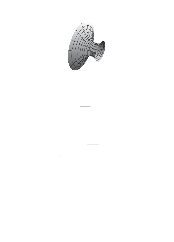
For small k an elliptic curve looks more or less like a circle, but as k > 0 it is deformed
into a more interesting shape. When k
→ 1 it tends to a parabola (see Fig. 3.1).
Only the part of the curve with real x between 1 and
−1 has a physical significance in
this application. But, as usual, to understand any algebraic curve it helps to analytically
continue into the complex plane. The surprising thing is that the curve is then a torus; this
follows from the double periodicity of sn, which we prove below.
Imaginary time
15
–1.0
–0.5
–0.5
0.5
1.0
–1.0
0.5
1.0
x
x
Fig. 3.1
Elliptic curves.
3.3.1
Addition formula
Suppose x
1
is the position of the pendulum after a time t
1
has elapsed, assuming that at
time zero, x = 0 as well. Similarly, let x
2
be the position at some time t
2
. If t
3
= t
1
+ t
2
,
and x
3
is the position at time t
3
, it should not be surprising that x
3
can be found once we
know x
1
and x
2
. What is surprising is that x
3
is an algebraic function of the positions. This
is because of the addition formula for elliptic functions:
x
1
0
dy
(1
− y
2
)(1
− k
2
y
2
)
+
x
2
0
dy
(1
− y
2
)(1
− k
2
y
2
)
=
x
3
0
dy
(1
− y
2
)(1
− k
2
y
2
)
x
3
=
x
1
(1
− x
2
2
)(1
− k
2
x
2
2
) + x
2
(1
− x
2
1
)(1
− k
2
x
2
1
)
1
− k
2
x
2
1
x
2
2
If k = 0, this is just the addition formula for sines:
sin[θ
1
+ θ
2
] = sin θ
1
1
− sin
2
θ
2
+ sin θ
2
1
− sin
2
θ
1
.
This operation x
1
, x
2
→ x
3
satisfies the conditions for an abelian group. The point of
stable equilibrium x = 0, ˙x = 1 is the identity element. The inverse of x
1
is just
−x
1
. You can
have fun trying to prove algebraically that the above operation is associative. (Or die trying.)
The replacement t
→ it has the effect of reversing the sign of the potential in Newton’s
equations, ¨
q =
−V
(q). In our case, ¨
θ =
− sin θ, it amounts to reversing the direction of
the gravitational field. In terms of co-ordinates, this amounts to θ
→ θ + π. Under the
transformations t
→ it, θ → θ + π, the conservation of energy

16
The simple pendulum
k
2
=
˙
θ
2
4
+ sin
2
θ
2
goes over to
1
− k
2
=
˙
θ
2
4
+ sin
2
θ
2
The quantity k
=
√
1
− k
2
is called the complementary modulus. In summary, the simple
pendulum has a symmetry
t
→ it, θ → θ + π, k → k
This transformation maps an oscillation of small amplitude (small k) to one of large
amplitude (k close to 1).
This means that if we analytically continue the solution of the pendulum into the com-
plex t-plane, it must be periodic with period 4K(k) in the real direction and 4K(k
) in the
imaginary direction.
3.4.1
The Case of
H = 1
The minimum value of energy is zero and the maximum value for an oscillation is 2. Exactly
half way is the oscillation whose energy is 1; the maximum angle is
π
2
. This orbit is invariant
under the above transformation that inverts the potential: either way you look at it, the
pendulum bob is horizontal at maximum deflection. In this case, the real and imaginary
periods are of equal magnitude.
Landen, and later Gauss, found a surprising symmetry for the elliptic integral K(k) that
allows a calculation of its value by iterating simple algebraic operations. In our context it
means that the period of a pendulum is unchanged if the energy H and angular frequency ω
are changed in a certain way that decreases their values. By iterating this we can make the
energy tend to zero, but in this limit we know that the period is just 2π over the angular
frequency. In this section we do not set ω = 1 but we continue to factor out ml
2
from the
Lagrangian as before. Then the Lagrangian L =
1
2
˙
θ
2
− ω
2
[1
− cos θ] and H have dimensions
of the square of frequency.
Let us go back and look at the formula for the period:
T =
4
ω
K(k),
K(k) =
1
0
dx
(1
− x
2
)(1
− k
2
x
2
)
,
2k
2
=
H
ω
2
If we make the substitution
x = sin φ

The arithmetic-geometric mean
∗
17
this becomes
T =
4
ω
π
2
0
dφ
1
− k
2
sin
2
φ
That is,
T (ω, b) = 4
π
2
0
dφ
ω
2
cos
2
φ + b
2
sin
2
φ
where
b =
ω
2
−
H
2
Note that ω > b with ω
→ b implying H → 0. The surprising fact is that the integral
remains unchanged under the transformations
ω
1
=
ω + b
2
,
b
1
=
√
ωb
T (ω, b) = T (ω
1
, b
1
)
Exercise 3.1: Prove this identity. First put y = b tan φ to get T (ω, b) =
2
∞
−∞
dy
√
(ω
2
+y
2
)(b
2
+y
2
)
. Then make the change of variable y = z +
√
z
2
+ ωb.
This proof, due to Newman, was only found in 1985. Gauss’s and Landen’s proofs
were much clumsier. For further explanation, see McKean and Moll (1999).
That is, ω is replaced by the arithmetic mean and b by the geometric mean.
Recall that given two numbers a > b > 0, the arithmetic mean is defined by
a
1
=
a + b
2
and the geometric mean is defined as
b
1
=
√
ab
As an exercise it is easy to prove that in general a
1
≥ b
1
. If we iterate this
transformation,
a
n
+1
=
a
n
+ b
n
2
,
b
n
+1
=
a
n
b
n
the two sequences converge to the same number, a
n
→ b
n
as n
→ ∞. This limiting value is
called the Arithmetic-Geometric Mean AGM(a, b).
Thus, the energy of the pendulum tends to zero under this iteration applied to ω and b,
since ω
n
→ b
n
; and the period is the limit of
2π
ω
n
:
T (ω, b) =
2π
AGM(ω, b)

18
The simple pendulum
The convergence of the sequence is quite fast, and gives a very accurate and elementary
way to calculate the period of a pendulum, i.e., without having to calculate any integral.
3.5.1
The arithmetic-harmonic mean is the geometric mean
Why would Gauss have thought of the arithmetic-geometric mean? This is perhaps puzzling
to a modern reader brought up on calculators. But it is not so strange if you know how to
calculate square roots by hand.
Recall that the harmonic mean of a pair of numbers is the reciprocal of the mean of
their reciprocals. That is
HM(a, b) =
1
1
2
1
a
+
1
b
=
2ab
a + b
Using (a + b)
2
> 4ab, it follows that
a
+b
2
> HM(a, b). Suppose that we define an iterative
process whereby we take the successive arithmetic and harmonic means:
a
n
+1
=
a
n
+ b
n
2
,
b
n
+1
= HM(a
n
, b
n
)
These two sequences approach each other, and the limit can be defined to be the
arithmetic-harmonic mean (AHM).
AHM(a, b) = lim
n
→∞
a
n
In other words, AHM(a, b) is defined by the invariance properties
AHM(a, b) = AHM
a + b
2
, HM(a, b)
,
AHM(λa, λb) = λAHM(a, b)
What is this quantity? It is none other than the geometric mean! Simply verify that
√
ab =
a + b
2
2ab
a + b
Thus iterating the arithmetic and harmonic means with 1 is a good way to calculate the
square root of any number. (Try it.)
Now you see that it is natural to wonder what we would get if we do the same thing
one more time, iterating the arithmetic and the geometric means.
AGM(a, b) = AGM
a + b
2
,
√
ab
I don’t know if this is how Gauss discovered it, but it is not such a strange idea.
Exercise 3.2: Relate the harmonic-geometric mean, defined by the invariance
below to the AGM.
HGM(a, b) = HGM
2ab
a + b
,
√
ab

Doubly periodic functions
∗
19
We are led to the modern definition: an elliptic function is a doubly periodic analytic func-
tion of a complex variable. We allow for poles, but not branch cuts: thus, to be precise, an
elliptic function is a doubly periodic meromorphic function of a complex variable.
f (z + m
1
τ
1
+ m
2
τ
2
) = f (z)
for integer m
1
, m
2
and complex numbers τ
1
, τ
2
which are called the periods. The points at
which f takes the same value form a lattice in the complex plane. Once we know the values
of f in a parallelogram whose sides are τ
1
and τ
2
, we will know it everywhere by translation
by some integer linear combination of the periods. In the case of the simple pendulum
above, one of the periods is real and the other is purely imaginary. More generally, they
could both be complex numbers; as long as the area of the fundamental parallelogram is
non-zero, we will get a lattice. By a rotation and a rescaling of the variable, we can always
choose one of the periods to be real. The ratio of the two periods
τ =
τ
2
τ
1
is thus the quantity that determines the shape of the lattice. It is possible to take some
rational function and sum over its values at the points z + m
1
τ
1
+ m
2
τ
2
to get a doubly
periodic function, provided that this sum converges. An example is
P
(z) =
−2
∞
m
1
,m
2
=−∞
1
(z + m
1
τ
1
+ m
2
τ
2
)
3
The power 3 in the denominator is the smallest one for which this sum converges; the
factor of
−2 in front is there to agree with some conventions. It has triple poles at the
origin and all points obtained by translation by periods m
1
τ
1
+ m
2
τ
2
. It is the derivative of
another elliptic function called
P, the Weierstrass elliptic function. It is possible to express
the Jacobi elliptic functions in terms of the Weierstrass function; these two approaches
complement each other. See McKean and Moll (1999) for more on these matters.
Problem 3.3: Show that the perimeter of the ellipse
x
2
a
2
+
y
2
b
2
= 1 is equal to
4a
1
0
1−k
2
x
2
1−x
2
dx, where k =
1
−
b
2
a
2
.
Problem 3.4: Using the change of variable x →
1
√
1−k
2
x
2
, show that K(k
) =
1
k
1
dx
√
[x
2
−1][1−k
2
x
2
]
.
Problem 3.5: Calculate the period of the pendulum with ω = 1, H = 1 by
calculating the arithmetic-geometric mean. How many iterations do you need
to get an accuracy of five decimal places for the AGM?
Problem 3.6**: What can you find out about the function defined by the
following invariance property?
AAGM(a, b) = AAGM
a + b
2
, AGM(a, b)

This page intentionally left blank

Much of mechanics was developed in order to understand the motion of planets. Long before
Copernicus, many astronomers knew that the apparently erratic motion of the planets can
be simply explained as circular motion around the Sun. For example, the Aryabhateeyam
written in ad 499 gives many calculations based on this model. But various religious taboos
and superstitions prevented this simple picture from being universally accepted. It is ironic
that the same superstitions (e.g., astrology) were the prime cultural motivation for studying
planetary motion. Kepler himself is a transitional figure. He was originally motivated by
astrology, yet had the scientific sense to insist on precise agreement between theory and
observation.
Kepler used Tycho Brahe’s accurate measurements of planetary positions to find a set of
important refinements of the heliocentric model. The three laws of planetary motion that he
discovered started the scientific revolution which is still continuing. We will rearrange the
order of presentation of the laws of Kepler to make the logic clearer. Facts are not always
discovered in the correct logical order: reordering them is essential to understanding them.
The orbit of a planet lies on a plane which contains the Sun
We may call this the zeroth law of planetary motion: this is a significant fact in itself. If the
direction of angular momentum is preserved, the orbit would have to lie in a plane. Since
L = r × p, this plane is normal to the direction of L. In polar co-ordinates in this plane,
the angular momentum is
L = mr
2
dφ
dt
that is, the moment of inertia times the angular velocity. In fact, all the planetary orbits lie
on the same plane to a good approximation. This plane is normal to the angular momentum
of the original gas cloud that formed the solar system.
The line connecting the planet to the Sun sweeps equal areas
in equal times
This is usually called the second law of Kepler. Since the rate of change of this area is
r
2
2
dφ
dt
,
this is the statement that
r
2
dφ
dt
= constant
22
The Kepler problem
This can be understood as due to the conservation of angular momentum. If the force
is always directed towards the Sun, this can be explained.
Planets move along elliptical orbits with the Sun at a focus
This is the famous first law of Kepler. It is significant that the orbit is a closed curve and
that it is periodic: for most central potentials neither statement is true.
An ellipse is a curve on the plane defined by the equation, in polar co-ordinates r, φ
ρ
r
= 1 + cos φ
For an ellipse, the parameter must be between 0 and 1 and is called the eccentricity.
It measures the deviation of an ellipse from a circle: if = 0 the curve is a circle of radius
ρ. In the opposite limit
→ 1 (keeping ρ fixed) it approaches a parabola. The parameter ρ
measures the size of the ellipse.
A more geometrical description of the ellipse is this: Choose a pair of points on the plane
F
1
, F
2
, the focii. If we let a point move on the plane such that the sum of its distances to
F
1
and F
2
is a constant, it will trace out an ellipse.
Exercise 4.1: Derive the equation for the ellipse above from this geometrical
description. (Choose the origin of the polar co-ordinate system to be F
1
. What
is the position of the other focus?)
The line connecting the two farthest points on an ellipse is called its major
axis; this axis passes through the focii. The perpendicular bisector to the major
axis is the minor axis. If these are equal in length, the ellipse is a circle; in this
case the focii coincide. Half of the length of the major axis is called a usually.
Similarly, the semi-minor axis is called b.
Exercise 4.2: Show that the major axis is
2ρ
1−
2
and that the eccentricity is
=
1
−
b
2
a
2
.
The eccentricity of planetary orbits is quite small: a few percent. Comets,
some asteroids and planetary probes have very eccentric orbits. If the eccen-
tricity is greater than one, the equation describes a curve that is not closed,
called a hyperbola. In the Principia, Newton proved that an elliptical orbit
can be explained by a force directed towards the Sun that is inversely pro-
portional to the square of distance. Where did he get the idea of a force
inversely proportional to the square of distance? The third law of Kepler provides
a clue.
The ratio of the cube of the semi-major axis to the square
of the period is the same for all planets
It took 17 years of hard work for Kepler to go from the second Law to this third law. Along
the way, he considered and discarded many ideas on planetary distances that came from
astrology and Euclidean geometry (Platonic solids).

The shape of the orbit
23
If, for the moment, we ignore the eccentricity (which is anyway small) and consider just
a circular orbit of radius r, this is saying that
T
2
∝ r
3
We already know that the force on the planet must be pointed toward the Sun, from the
conservation of angular momentum. What is the dependence of the force on distance that
will give this dependence of the period? Relating the force to the centripetal acceleration,
m
v
2
r
= F (r)
Now, v = r ˙
θ and ˙
θ =
2π
T
for uniform circular motion. Thus
T
2
∝
r
F (r)
So we see that F (r)
∝
1
r
2
.
Hooke, a much less renowned scientist than Newton, verified using a mechanical model
that orbits of particles in this force are ellipses. He made the suggestion to Newton, who
did not agree at that time. Later, while he was writing the Principia, Newton discovered a
marvelous proof of this fact using only geometry (no calculus). Discoveries are often made
by a collaborative process involving many people, not just a lone genius.
From the fact that the ratio
T
2
r
3
is independent of the planet, we can conclude that the
acceleration is independent of the mass of the planet: that the force is proportional to the
product of masses. Thus we arrive at Newton’s Law of Gravity:
The gravitational force on a body due to another is pointed along the line
connecting the bodies; it has magnitude proportional to the product of masses
and inversely to the square of the distance.
We now turn to deriving the shape of a planetary orbit from Newton’s law of gravity. The
Lagrangian is, in plane polar co-ordinates centered at the Sun,
L =
1
2
m
˙r
2
+ r
2
˙
φ
2
+
GM m
r
From this we deduce the momenta
p
r
= m ˙r,
p
φ
= mr
2
˙
φ
and the hamiltonian
H =
p
2
r
2m
+
p
2
φ
2mr
2
−
GM m
r
24
The Kepler problem
Since
∂H
∂φ
= 0, it follows right away that p
φ
is conserved.
H =
p
2
r
2m
+ V (r)
where
V (r) =
p
2
φ
2mr
2
−
GM m
r
is an effective potential, the sum of the gravitational potential and the kinetic energy due
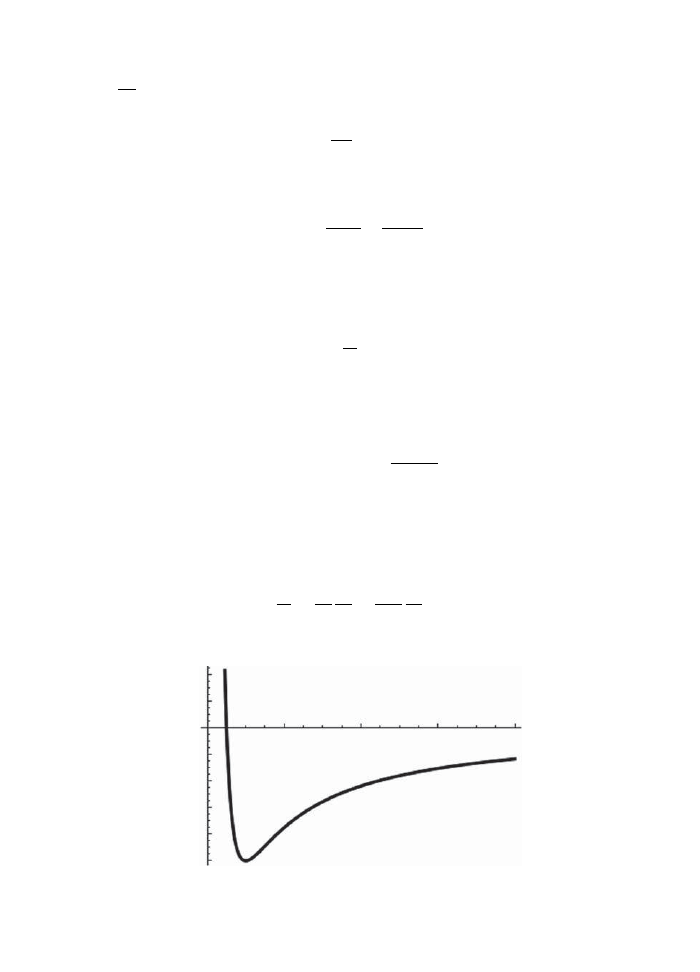
to angular motion (see Fig. 4.1).
So,
˙r =
p
r
m
˙
p
r
=
− V
(r)
Right away, we see that there is a circular orbit at the minimum of the potential:
V
(r) = 0 =
⇒ r =
p
2
φ
GM m
2
More generally, when H < 0, we should expect an oscillation around this minimum,
between the turning points, which are the roots of H
− V (r) = 0. For H > 0 the particle
will come in from infinity and, after reflection at a turning point, escape back to infiinity.
The shape of the orbit is given by relating r to φ. Using
dr
dt
=
dφ
dt
dr
dφ
=
p
φ
mr
2
dr
dφ
2
–0.10
–0.08
–0.06
–0.04
–0.02
0.02
0.04
4
6
8
Fig. 4.1
The potential of the Kepler problem.
The shape of the orbit
25
This suggests the change of variable
u = A +
ρ
r
, =
⇒
dr
dt
=
−
p
φ
mρ
du
dφ
=
−
p
φ
mρ
u
for some constants A, ρ that we will choose for convenience later. We can express the
conservation of energy
H =
1
2
m ˙r
2
+ V (r)
as
H =
p
2
φ
2mρ
2
u
2
+
p
2
φ
2mρ
2
(u
− A)
2
−
GM m
ρ
(u
− A)
2mρ
2
H
p
2
φ
= u
2
+ (u
− A)
2
−
2GM m
2
ρ
p
2
φ
(u
− A)
We can now choose the constants so that the term linear in u cancels out
A =
−1, ρ =
p
2
φ
GM m
2
and
u
2
+ u
2
=
2
2
= 1 +
2p
2
φ
H
(GM )
2
m
3
A solution is now clear
u = cos φ
or
ρ
r
= 1 + cos φ
This is the equation for a conic section of eccentricity . If H < 0, so that the planet
cannot escape to infinity, this is less than one, giving an ellipse as the orbit.
Problem 4.3: Show that among all Kepler orbits of the same angular momen-
tum, the circle has the least energy.
Problem 4.4: What would be the shape of the orbit if the gravitational poten-
tial had a small correction that varies inversely with the square of the distance?
Which of the laws of planetary motion would still hold?

26
The Kepler problem
Problem 4.5: The equation of motion of a classical electron orbiting a nucleus
is, including the effect of radiation,
d
dt
[ ˙
r + τ∇U] + ∇U = 0, U = −
k
r
The positive constants τ, k are related to the charge and mass of the particles.
Show that the orbits are spirals converging to the center. This problem was
solved in Rajeev (2008).

If the distance between any two points on a body remains constant as it moves, it is a
rigid body. Any configuration of the rigid body can be reached from the initial one by a
translation of its center of mass and a rotation around it. Since we are mostly interested in
the rotational motion, we will only consider the case of a body on which the total force is
zero: the center of mass moves at a constant velocity. In this case we can transform to the
reference frame in which the center of mass is at rest: the origin of our co-ordinate system
can be placed there. It is not hard to put back in the translational degree of freedom once
rotations are understood.
The velocity of one of the particles making up the rigid body can be split as
v = Ω × r
The vector
Ω is the angular velocity: its direction is the axis of rotation and its magnitude
is the rate of change of its angle. The kinetic energy of this particle inside the body is
1
2
[
Ω × r]
2
ρ(
r)d
3
r
Here ρ(
r) is the mass density at the position of the particle; we assume that it occupies
some infinitesimally small volume d
3
r. Thus the total rotational kinetic energy is
T =
1
2
[
Ω × r]
2
ρ(
r)d
3
r
Now, (
Ω × r)
2
= Ω
2
r
2
− (Ω · r)
2
= Ω
i
Ω
j
r
2
δ
ij
− r
i
r
j
, so we get
T =
1
2
Ω
i
Ω
j
ρ(
r)
r
2
δ
ij
− r
i
r
j
d
3
r
Define the moment of inertia to be the symmetric matrix
I
ij
=
ρ(
r)
r
2
δ
ij
− r
i
r
j
d
3
r

28
The rigid body
Thus
T =
1
2
Ω
i
Ω
j
I
ij
Being a symmetric matrix, there is an orthogonal co-ordinate system in which the
moment of inertia is diagonal:
T =
1
2
I
1
Ω
2
1
+ I
2
Ω
2
2
+ I
3
Ω
2
3
The eigenvalues I
1
, I
2
, I
3
are called the principal moments of inertia. They are positive
numbers because I
ij
is a positive matrix, i.e., u
T
Iu
≥ 0 for any u.
Exercise 5.1: Show that the sum of any two principal moments is greater than
or equal to the third one. I
1
+ I
2
≥ I
3
etc.
The shape of the body, and how mass is distributed inside it, determines the moment
of inertia. The simplest case is when all three are equal. This happens if the body is highly
symmetric: a sphere, a regular solid such as a cube. The next simplest case is when two
of the moments are equal and the third is different. This is a body that has one axis of
symmetry: a cylinder, a prism whose base is a regular polygon etc. The most complicated
case is when the three eigenvalues are all unequal. This is the case of the asymmetrical top.
The angular momentum of a small particle inside the rigid body is
dM
r × v =
ρ(
r)d
3
r
r × (Ω × r)
Using the identity
r × (Ω × r) = Ωr
2
− r (Ω · r) we get the total angular momentum of the
body to be
L =
ρ(
r)[r
2
Ω − r (Ω · r)]d
3
r
In terms of components
L
i
= I
ij
Ω
j
Thus the moment of inertia relates angular velocity to angular momentum, just as mass
relates velocity to momentum. The important difference is that moment of inertia is a
matrix so that
L and Ω do not have to point in the same direction. Recall that the rate
of change of angular momentum is the torque, if they are measured in an inertial reference
frame.
Euler’s equations
29
Now here is a tricky point. We would like to use a co-ordinate system in which the mo-
ment of inertia is a diagonal matrix; that would simplify the relation of angular momentum
to angular velocity:
L
1
= I
1
Ω
1
etc. But this may not be an inertial co-ordinate system, as its axes have to rotate with
the body. So we must relate the change of a vector (such as
L) in a frame that is fixed
to the body to an inertial frame. The difference between the two is a rotation of the body
itself, so that
d
L
dt
inertial
=
d
L
dt
+
Ω × L
This we set equal to the torque acting on the body as a whole.
Even in the special case when the torque is zero the equations of motion of a rigid body
are non-linear, since
Ω and L are proportional to each other:
d
L
dt
+
Ω × L = 0
In the co-ordinate system with diagonal moment of inertia
Ω
1
=
L
1
I
1
these become
dL
1
dt
+ a
1
L
2
L
3
= 0,
a
1
=
1
I
2
−
1
I
3
dL
2
dt
+ a
2
L
3
L
1
= 0,
a
2
=
1
I
3
−
1
I
1
dL
3
dt
+ a
3
L
1
L
2
= 0,
a
3
=
1
I
1
−
1
I
2
These equations were originally derived by Euler. Clearly, if all the principal moments of
inertia are equal, these are trivial to solve:
L is a constant.
The next simplest case
I
1
= I
2
= I
3
is not too hard either. Then a
3
= 0 and a
1
=
−a
2
.

30
The rigid body
It follows that L
3
is a constant. Also, L
1
and L
2
precess around this axis:
L
1
= A cos ωt,
L
2
= A sin ωt
with
ω = a
1
L
3
An example of such a body is the Earth. It is not quite a sphere, because it bulges at
the equator compared to the poles. The main motion of the Earth is its rotation around the
north–south axis once every 24 hours. But this axis itself precesses once every 26,000 years.
This means that the axis was not always aligned with the Pole Star in the distant past.
Also, the times of the equinoxes change by a few minutes each year. As early as 280 bc
Aristarchus described this precession of the equinoxes. It was Newton who finally explained
it physically.
The general case of unequal moments can be solved in terms of Jacobi elliptic functions; in
fact, these functions were invented for this purpose. But before we do that it is useful to
find the constants of motion. It is no surprise that the energy
H =
1
2
I
1
Ω
2
1
+
1
2
I
2
Ω
2
2
+
1
2
I
3
Ω
2
3
=
L
2
1
2I
1
+
L
2
2
2I
2
+
L
2
3
2I
3
is conserved. You can verify that the magnitude of angular momentum is conserved as well:
L
2
= L
2
1
+ L
2
2
+ L
2
3
Exercise 5.2: Calculate the time derivatives of H and L
2
and verify that they
are zero.
Recall that
sn
= cn dn,
cn
=
−sn dn, dn
=
−k
2
sn cn
with initial conditions
sn = 0,
cn = 1,
dn = 1,
at u = 0
Moreover
sn
2
+ cn
2
= 1,
k
2
sn
2
+ dn
2
= 1
Make the ansatz
L
1
= A
1
cn(ωt, k)
L
2
= A
2
sn(ωt, k),
L
3
= A
3
dn(ωt, k)

Jacobi’s solution
31
We get conditions
−ωA
1
+ a
1
A
2
A
3
= 0
ωA
2
+ a
2
A
3
A
1
= 0
−ωk
2
A
3
+ a
3
A
1
A
2
= 0
We want to express the five constants A
1
, A
2
, A
3
, ω, k that appear in the
solution in terms of the five physical parameters H, L, I
1
, I
2
, I
3
. Some serious
algebra will give
1
ω =
(I
3
− I
2
)(L
2
− 2HI
1
)
I
1
I
2
I
3
k
2
=
(I
2
− I
1
)(2HI
3
− L
2
)
(I
3
− I
2
)(L
2
− 2HI
1
)
and
A
2
=
(2HL
3
− L
2
)I
2
I
3
− I
2
etc.
The quantum mechanics of the rigid body is of much interest in molecular
physics. So it is interesting to reformulate this theory in a way that makes the
passage to quantum mechanics more natural. The Poisson brackets of angular
momentum derived later give such a formulation.
Problem 5.3: Show that the principal moments of inertia of a cube of constant
density are all equal. So, there is a sphere of some radius with the same moment
of inertia and density as the cube. What is its radius as a multiple of the side
of the cube?
Problem 5.4: More generally, show that the moment of inertia is proportional
to the identity matrix for all of the regular solids of Euclidean geometry. In ad-
dition to the cube, these are the tetrahedron, the octahedron, the dodecahedron
and the icosahedron. A little group theory goes a long way here.
Problem 5.5: A spheroid is the shape you get by rotating an ellipse around
one of its axes. If it is rotated around the major (minor) axis you get a pro-
late (oblate) spheroid. Find the principal moments of inertia for each type of
spheroid.
1
We can label our axes such that I
3
> I
2
> I
1
.

This page intentionally left blank

6
Geometric theory of ordinary
differential equations
Any problem in classical mechanics can be reduced to a system of ordinary differential
equations
dx
μ
dt
= V
μ
(x),
for μ = 1,
· · · , n
In general V
μ
can depend on the independent variable t in addition to x
μ
. But we will avoid
this by a cheap trick: if V
μ
(x, t) does depend on time, we will add an extra variable x
n
+1
and an extra component V
n
+1
(x
1
,
· · · , x
n
+1
) = 1. This says that x
n
+1
= t up to a constant,
so we get back the original situation. Similarly, if we have to solve an equation of order
higher than one, we can just add additional variables to bring it to this first order form.
Also, we will assume in this chapter that V
μ
are differentiable functions of x
μ
. Singular
cases have to be studied by making a change of variables that regularizes them (i.e., brings
them to non-singular form).
For more on this geometric theory, including proofs, study the classic texts (Lefschetz,
1977; Arnold, 1978).
We can regard the dependent variables as the co-ordinates of some space, called the phase
space.
1
The number of variables n is then the dimension of the phase space. Given the
variables x
μ
at one instant of the independent variable (“time”), it tells us how to deduce
their values a small time later: x
μ
(t + dt) = x
μ
(t) + V
μ
(x)dt. It is useful to have a physical
picture: imagine a fluid filling the phase space, and V
μ
(x) is the velocity of the fluid element
at x
μ
. At the next instant it has moved to a new point where there is a new value of the
velocity, which then tells it where to be at the instant after and so on. Thus, V
μ
defines
a vector field in phase space. Through every point in phase spaces passes a curve which
describes the time evolution of that point: it is called the integral curve of the vector field
V
μ
. These curves intersect only at a point where the vector field vanishes: these are fixed
points.
1
By “space” we mean “differential manifold.” It is a tradition in geometry to label co-ordinates by an
index that sits above (superscript) instead of a subscript. You can tell by the context whether x
2
refers to
the second component of some co-ordinate or the square of some variable x.
34
Geometric theory of ordinary differential equations
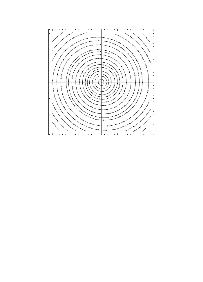
3
2
1
0
–1
–2
–3
–3
–2
–1
0
x
2
x
1
1
2
3
Fig. 6.1
Orbits of the damped harmonic oscillator.
Example 6.1: The equation of a damped simple harmonic oscillator
¨
q + γ ˙
q + ω
2
q = 0
is reduced to first order form by setting x
1
= q, x
2
= ˙
q so that
dx
1
dt
= x
2
,
dx
2
dt
=
−γx
2
− ω
2
x
1
The phase space in this case is the plane. The origin is a fixed point. The integral
curves are spirals towards the origin (see Fig. 6.1).
The simplest example of a differential manifold is Euclidean space. By introducing a
Cartesian co-ordinate system, we can associate to each point an ordered tuple of real num-
bers (x
1
, x
2
,
· · · , x
n
), its co-ordinates. Any function f : M
→ R can then be viewed as a
function of the co-ordinates. We know what it means for a function of several variables to
be smooth, which we can use to define a smooth function in Euclidean space. But there

Differential manifolds
35
is nothing sacrosanct about a Cartesian co-ordinate system. We can make a change of
variables to a new system
y
μ
= φ
μ
(x)
as long as the new co-ordinates are still smooth, invertible functions of the old. In particular,
this means that the matrix (Jacobian) J
μ
ν
=
∂φ
μ
∂x
ν
has non-zero determinant everywhere. In
fact, if we had the inverse function x
μ
= ψ
μ
(y) its Jacobian would be the inverse:
∂φ
μ
∂x
ν
∂ψ
ν
∂y
σ
= δ
μ
σ
But it turns out to be too strict to demand that the change of co-ordinates be smooth
everywhere: sometimes we want co-ordinates systems that are only valid in some subset of
Euclidean space.
Example 6.2: The transformation to the polar co-ordinate system on the plane
x
1
= r cos θ,
x
2
= r sin θ
is not invertible because θ and θ + 2π correspond to the same point. So we must
restrict to the range 0
≤ θ < 2π. Thus the polar system is valid on the plane
with the positive x
1
-axis removed. To cover all of Euclidean space, we must use,
in addition, another polar co-ordinate system with a different origin and an axis
that does not intersect this line. Most points will belong to both co-ordinate
patches, and the transformation between them is smooth. Together they cover
all of the plane.
We can abstract out of this the definition of a far-reaching concept. A dif-
ferential manifold is a set which can be written as a union of M =
α
U
α
; each
“co-ordinate patch” U
α
is in one–one correspondence x
α
: U
α
→ R
n
with some
domain of Euclidean space R
n
. Moreover, there are smooth invertible functions
(“co-ordinate transformations”) φ
αβ
: R
n
→ R
n
such that
x
α
= φ
αβ
(x
β
)
The point of this is that locally (in the neighborhood of a point) a differentiable
manifold looks like Euclidean space. But each such patch can be attached to
another, such that globally it looks very different. A sphere, a torus, a Klein
bottle are all examples of such manifolds.
Example 6.3: A sphere can be covered by two co-ordinate patches: one ex-
cluding the south pole and the other excluding the north pole. To get the
“stereographic co-ordinate” x of a point P
= S in the first patch, draw a straight
line that connects the south pole to P ; extend it until it meets the tangent plane
to the north pole (see Fig. 6.2). N itself has zero as the co-ordinate. As you move
closer to the south pole, the co-ordinate x moves off to infinity. That is why S
itself has to be excluded. Interchange N and S to get the other co-ordinate
patch.
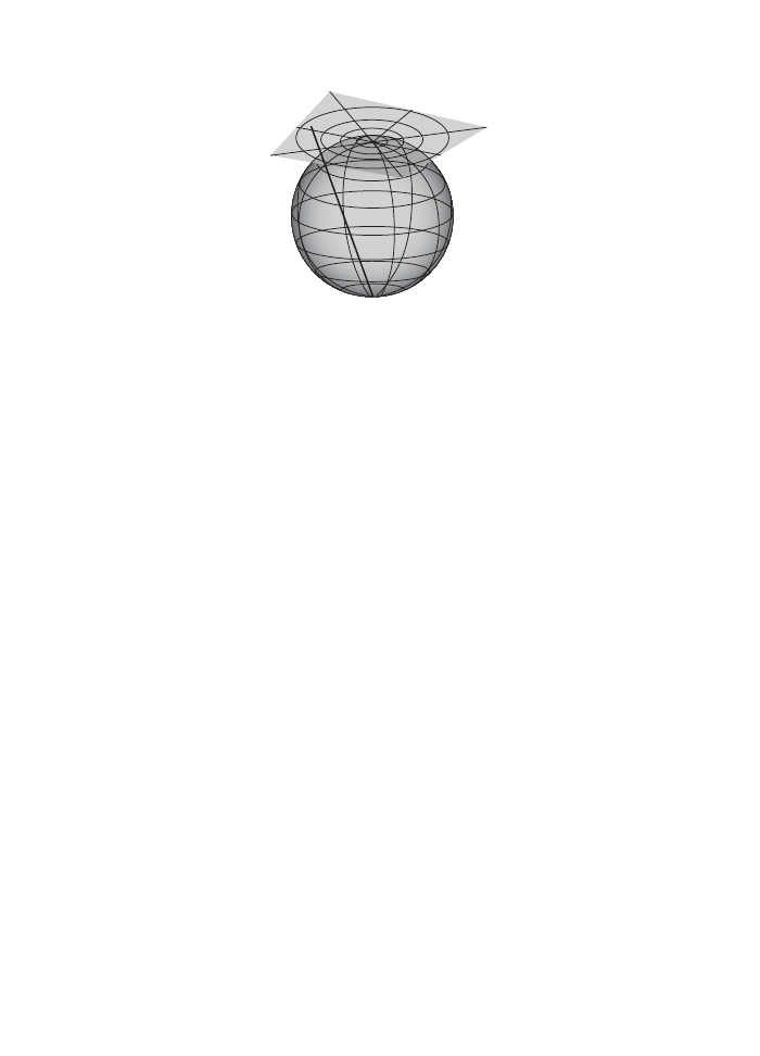
36
Geometric theory of ordinary differential equations
S
P
x(P)
Fig. 6.2
The stereographic co-ordinate on the sphere.
The basic object on a differential manifold is a smooth function; i.e., a function f : M
→ R
such that its restriction to each path is a smooth function of the co-ordinates. The set
of functions in the space M form a commutative algebra over the real number field: we
can multiply them by constants (real numbers); and we can multiply two functions to get
another:
f g(x) = f (x)g(x)
A derivation of a commutative algebra A is a linear map V : A
→ A that satisfies the
Leibnitz rule
V (f g) = (V f )g + f V (g)
We can add two derivations to get another. Also we can multiply them by real numbers
to get another derivation. The set of derivations of a commutative algebra form a module
over A; i.e., the left multiplication f V is also a derivation. In our case of functions in a
space, each component of the vector field is multiplied by the scalar f .
In this case, a derivation is the same as a first order differential operator or vector field:
V f = V
μ
∂
μ
f
The coefficient of the derivative along each co-ordinate is the component of the vector field
in the direction.
The product of two derivations is not in general a derivation: it does not satisfy the
Leibnitz rule:
V (W (f g)) = V ((W f )g + f W (g))
= V (W (f ))g + 2(W f )(V g) + f V (W (g))

Vector fields as derivations
37
But the commutator of two derivations, defined as
[V, W ] = V W
− W V
is always another derivation:
V (W (f g))
− W (V (fg)) = V (W (f))g + fV (W (g)) − W (V (f))g − fW (V (g))
In terms of components,
[V, W ]
μ
= V
ν
∂
ν
W
μ
− W
ν
∂
ν
V
μ
We sum over repeated indices as is the convention in geometry. The commutator of
vector fields satisfies the identities
[V, W ] + [W, V ] = 0
[[U, V ], W ] + [[V, W ], U ] + [[W, U ], V ] = 0
Any algebra that satisfies these identities is called a Lie algebra. The set of vector fields
on a manifold is the basic example. Lie algebras describe infinitesimal transformations.
Many of them are of great interest in physics, as they describe symmetries. More on this
later.
Example 6.4: The vector field
V =
∂
∂x
generates translations along x. Its integral curve is x(t) = x
0
+ t.
Example 6.5: On the other hand,
W = x
∂
∂x
generates scaling. That is, its integral curve is
x(u) = e
u
x
0
We see that these two vector fields have the commutator
[V, W ] = V
Example 6.6: Infinitesimal rotations around the three Cartesian axes on R
3
are described by the vector fields
L
x
=
−y
∂
∂z
+ z
∂
∂y
,
L
y
=
−z
∂
∂x
+ x
∂
∂z
,
L
z
=
−x
∂
∂y
+ y
∂
∂x

38
Geometric theory of ordinary differential equations
They satisfy the commutation relations
[L
x
, L
y
] = L
z
,
[L
y
, L
z
] = L
x
,
[L
z
, L
x
] = L
y
Given two vector fields V, W , we can imagine moving from x
0
along the integral
curve of V for a time δ
1
and then along that of W for some time δ
2
. Now suppose
we reverse the order by first going along the integral curve of W for a time δ
2
and then along that of V for a time δ
2
. The difference between the two endpoints
is order δ
1
δ
2
, but is not in general zero. It is equal to the commutator:
[V
ν
∂
ν
W
μ
− W
ν
∂
ν
V
μ
] δ
1
δ
2
Thus, the commutator of vector fields, which we defined above algebraically,
has a geometric meaning as the difference between moving along the integral
curves in two different ways. Such an interplay of geometry and algebra en-
riches both fields. Usually geometry helps us imagine things better or relate the
mathematics to physical situations. The algebra is more abstract and allows
generalizations to new physical situations that were previously unimaginable.
For example, the transition from classical to quantum mechanics involves non-
commutative algebra. These days we are circling back and constructing a new
kind of geometry, non-commutative geometry, which applies to quantum systems
(Connes, 1994).
A point at which a vector field vanishes is called a fixed point. An orbit that starts there
stays there. Thus equilibrium points of dynamical systems are fixed points. It is interesting
to ask what happens if we are close to but not at a fixed point. Being differentiable, the
components of the vector field can be expanded in a Taylor series. It makes sense to choose
a co-ordinate system whose origin is the fixed point. Thus
V
μ
(x) = V
μ
ν
x
ν
+ O(x
2
)
The matrix V
is the main actor now. Suppose it can be diagonalized: there is an invertible
real matrix S such that V
= S
−1
ΛS, and Λ is diagonal. Then we can make a linear change
of co-ordinates to bring the equations to the form
˙x
μ
= λ
μ
x
μ
+ O(x
2
)
The integral curves are,
x
μ
(t)
≈ A
μ
e
λ
μ
t
This remains small, and the approximation remains valid, as long as λ
μ
and t have opposite
signs; or if t is small. If all the eigenvalues are real and negative, we say that the fixed point
is stable. Forward time evolution will drive any point near the fixed point even closer to

Fixed points
39
it. If all the eigenvalues are positive, we have an unstable fixed point. Although for small
positive times the orbit is nearby, V
does not have enough information to determine the
fate of the orbit for large times. Such unstable orbits can for example, be dense (come as
close as necessary to every point in phase space).
If some λ are positive and some are negative, there is a subspace of the tangent space
at the fixed point containing the stable directions and a complementary one containing the
unstable directions. There is a neighborhood of the fixed point which can then be expressed
as a product of a stable and an unstable submanifold. But as we move away from the
fixed point, these need not be submanifolds at all: they might intersect, or one (or both)
of them might be dense. What if some of the eigenvalues vanish? Then the dynamics in
those directions is determined by going to the next order in the Taylor expansion. Whether
those directions are stable or not depends on the sign of the second derivative of V in those
directions.
A physically important case is when the characteristic values are complex.
Example 6.7: Let us return to the damped harmonic oscillator 6.1. Clearly
x = 0 is a fixed point and
V
=
0
1
−ω
2
−γ
The eigenvalues are λ
±
=
−
γ
2
± i
ω
2
−
γ
2
4
. As long as γ > 0, ω >
γ
2
, the orbits
are spirals converging to the fixed points:
x
1
= e
−
γ
2
t
A sin
ω
2
−
γ
2
4
t + φ
Since V
is real, its complex eigenvalues must come in pairs: if λ is an eigen-
value, so will be λ
∗
. Each such pair is associated to a plane in the tangent space
at the fixed point. If Reλ < 0, the orbits spiral towards the fixed point as t
→ ∞.
So complex eigenvalues are stable if Reλ < 0 and unstable if Reλ > 0.
Problem 6.1: What are the orbits of the over-damped harmonic oscillator:
Example 6.1 with γ > 0, ω
2
<
γ
2
4
? What are the orbits when γ < 0 but ω
2
>
γ
2
4
?
Also, analyze the case where γ > 0, ω
2
>
γ
2
4
.
Problem 6.2: Consider the torus T = S
1
× S
1
. We can think of it as the set
of points on the plane modulo translation by integers. Define the vector field
V = (1, γ) where γ is a real number. Show that if γ =
m
n
(for co-prime m, n) is
a rational number, the orbit is a closed curve that winds m times around the
first circle and n times around the second circle. Also, that if γ is irrational, the
orbit is dense: every point on the torus is within a distance of some point on
the orbit, for any .
Problem 6.3: Consider a two-dimensional ODE with a fixed point at which
the characteristic polynomial of the Jacobi matrix has unequal roots. Recall
that in this case, there is a change of co-ordinates which will bring this matrix
to diagonal form. Plot the orbits in each of the following cases:

40
Geometric theory of ordinary differential equations
1. The roots are real and non-zero: cases when they are both positive, one is
positive and one negative and both are negative.
2. One root is zero and the cases when the other root is positive or negative.
3. If the roots are complex, they must be complex conjugates of each other.
Plot the orbits for the cases when the real part is positive, zero and negative.
Problem 6.4*: Let β(α)
d
dα
be a vector field on the real line with a double zero
at the origin:
β(α) = β
2
α
2
+ β
3
α
3
+ β
4
(α)α
4
β
2
= 0, β
3
are constants and β
4
(α) is a smooth function in some neighborhood
of the origin. Show that there is a change of variables
x(α) = x
1
α + x
3
(α)α
3
such that the vector field can be brought to the standard form
β(α)
d
dα
= [1 + λx] x
2
d
dx
,
λ =
β
3
β
2
2
Here, x
3
(α) should be a smooth function in a neighborhood of the origin.
We require that x
1
= 0 so that the change of variables α → x is invertible in
a neighborhood of the origin. It will reverse the orientation if x
1
< 0 and not
otherwise.
Solution
We get
β
2
α
2
+ β
3
α
3
+ β
4
(α)α
4
dx
dα
= x
2
(α) + λx
3
(α)
Equating terms of order α
2
β
2
x
1
= x
2
1
=
⇒ x
1
= β
2
In order α
3
we get
β
3
x
1
= λx
3
1
Putting these in and simplifying we get a differential equation
β
2
+ β
3
α + β
4
(α)α
2
x
3
(α) + β
2
β
4
(α) + x
3
(α)
α
+
αx
3
(α)[3β
4
(α)
− x
3
(α)]
−
β
3
α
2
x
3
(α)
2
β
2
2
3β
2
+ α
2
x
3
(α)
= 0
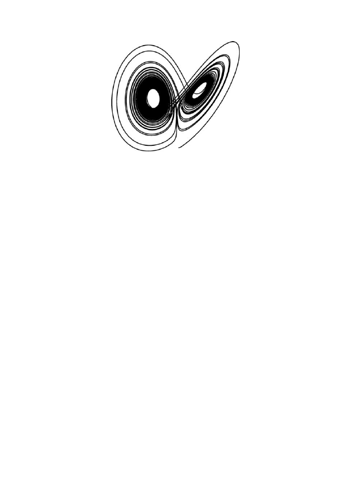
Fixed points
41
Fig. 6.3
The Lorenz system.
The singularity at α = 0 cancels out for the initial condition
x
3
(0) =
−β
4
(0)
yielding a solution in some neighborhood of α = 0. This problem arises in the
study of asymptotically free quantum field theories by G. ’t Hooft.
Problem 6.5: The Lorenz system is defined by
˙x = α(y
− x),
˙
y =
−xz + βx − y,
˙z = xy
− z
Write a computer program that solves it numerically and plots the integral
curves. Of special interest is to study the case β = 20 with α = 3 for the time
range 0 < t < 250 and initial condition x(0) = 0 = z(0), y(0) = 1. The orbit lies
on a submanifold called a strange attractor, shaped like the wings of a butterfly
(see Fig. 6.3). A small change in time can result in the system switching from
one wing to the other.

This page intentionally left blank

William Rowan Hamilton (1805–1865) was the Astronomer Royal for Ireland. In this capa-
city, he worked on two important problems of mathematical interest: the motion of celestial
bodies and the properties of light needed to design telescopes. Amazingly, he found that
the laws of mechanics and those of ray optics were, in the proper mathematical framework,
remarkably similar. But ray optics is only an approximation, valid when the wavelength of
light is small. He probably wondered in the mid nineteenth century: could mechanics be
the short wavelength approximation of some wave mechanics?
The discovery of quantum mechanics brought this remote outpost of theoretical physics
into the very center of modern physics.
Recall that to each co-ordinate q
i
we can associate a momentum variable,
p
i
=
∂L
∂ ˙
q
i
p
i
is said to be conjugate to q
i
. It is possible to eliminate the velocities and write the
equations of motion in terms of q
i
, p
i
. In this language, the equations will be a system of
first order ODEs. Recall that from the definition of the hamiltonian
L =
i
p
i
˙
q
i
− H
So if we view H(q, p) as a function of position and momentum, we get a formula for the
action
S =
i
p
i
˙
q
i
− H(q, p, t)
dt
Suppose we find the condition for the action to be an extremum, treating q
i
, p
i
as
independent variables:
δS =
i
δp
i
˙
q
i
+ p
i
d
dt
δq
i
− δp
i
∂H
∂p
i
− δq
i
∂H
∂q
i
dt = 0

44
Hamilton’s principle
We get the system of ODE
dq
i
dt
=
∂H
∂p
i
,
dp
i
dt
=
−
∂H
∂q
i
These are called Hamilton’s equations. They provide an alternative formulation of
mechanics.
Example 7.1: A particle moving on the line under a potential has
L =
1
2
m ˙
q
2
− V (q) and H =
p
2
2m
+ V (q)
It follows that
dq
dt
=
p
m
,
dp
dt
=
−V
(q)
Clearly, these are equivalent to Newton’s second law.
Example 7.2: For the simple pendulum
L =
1
2
˙
θ
2
− [1 − cos θ] , H =
p
2
θ
2
+ 1
− cos θ
In terms of the variable x =
1
k
sin
θ
2
L = 2k
2
˙x
2
1
− k
2
x
2
− x
2
It follows that
p =
∂L
∂ ˙x
= 4k
2
˙x
1
− k
2
x
2
,
H = 2k
2
1
− k
2
x
2
p
2
+ x
2
If we choose the parameter k such that H = 2k
2
the relation between p and
x becomes
p
2
=
1
− x
2
1
− k
2
x
2
This is another description of the elliptic curve, related rationally to the
more standard one:
y =
1
− k
2
x
2
p
4k
2
,
y
2
=
1
− x
2
1
− k
2
x
2
Example 7.3: A particle moving under a potential in three dimensions has
L =
1
2
m ˙
r
2
− V (r)
so that
H =
p
2
2m
+ V (
r)
˙
r =
p
m
,
˙
p = −∇V

Poisson brackets
45
For the Kepler problem
V (
r) = −
GM m
|r|
Being first order ODE, the solution for Hamilton’s equations is determined once the value
of (q
i
, p
i
) is known at one instant. The space M whose co-ordinates are (q
i
, p
i
) is the phase
space. Each point of phase space determines a solution of Hamilton’s equation, which we
call the orbit through that point. Hamilton’s equations tell us how a given point in phase
space evolves under an infinitesimal time translation: they define a vector field in the phase
space. By compounding such infinitesimal transformations, we can construct time evolution
over finite time intervals: the orbit is the integral curve of Hamilton’s vector field.
V
H
=
∂H
∂p
i
∂
∂q
i
−
∂H
∂q
i
∂
∂p
i
Since the state of the system is completely specified by a point in the phase space, any
physical observable must be a function f (q, p); that is, a function f : M
→ R of position
and momentum.
1
The hamiltonian itself is an example of an observable; perhaps the most
important one.
We can work out an interesting formula for the total time derivative of an observable:
df
dt
=
i
dq
i
dt
∂f
∂q
i
+
dp
i
dt
∂f
∂p
i
Using Hamilton’s equations this becomes
df
dt
=
i
∂H
∂p
i
∂f
∂q
i
−
∂H
∂q
i
∂f
∂p
i
Given any pair of observables, we define their Poisson bracket to be
{g, f} =
i
∂g
∂p
i
∂f
∂q
i
−
∂g
∂q
i
∂f
∂p
i
Thus
df
dt
=
{H, f}
1
Sometimes we would also allow an explicit dependence in time, but we ignore that possibility for the
moment.

46
Hamilton’s principle
A particular example is when f is one of the co-ordinates themselves:
{H, q
i
} =
∂H
∂p
i
,
{H, p
i
} = −
∂H
∂q
i
You may verify the canonical relations
{p
i
, p
j
} = 0 =
q
i
, q
j
,
p
i
, q
j
= δ
j
i
Here δ
j
i
=
1
if i = j
0
otherwise
is the Kronecker symbol.
Exercise 7.1: Show that the Poisson bracket satisfies the conditions for a Lie
algebra:
{f, g} + {g, f} = 0, {{f, g} , h} + {{g, h} , f} + {{h, f} , g} = 0
and in addition that
{f, gh} = {f, g} h + g {f, h}
Together these relations define a Poisson algebra.
The observables of quantum mechanics can still be thought of as functions in the phase
space. But then, the rule for multiplying observables is no longer the obvious one: it is
a non-commutative operation. Without explaining how it is derived, we can exhibit the
formula for this quantum multiplication law in the case of one degree of freedom:
f
∗g = fg −
i
2
∂f
∂p
∂g
∂q
−
∂f
∂q
∂g
∂p
+
1
2
i
2
2
∂
2
g
∂p
2
∂
2
f
∂q
2
−
∂
2
g
∂q
2
∂
2
f
∂p
2
+
· · ·
Or,
f
∗g = fg +
∞
r
=1
1
r!
−
i
2
r
∂
2r
g
∂p
r
∂
r
f
∂q
r
−
∂
r
g
∂q
r
∂
r
f
∂p
r
This is an associative, but not commutative, multiplication: (f
∗g)∗h = f∗(g∗h). (It can
be proved using a Fourier integral representation.) Note that the zeroth order term is the
usual multiplication and that the Poisson bracket is the first correction. In particular, in
quantum mechanics we have the Heisenberg commutation relations
[p, q] =
−i
where the commutator is defined as [p, q] = p
∗q − q∗p.

Canonical transformation
47
The constant functions are multiples of the identity in this
∗-product. We can define
the inverse, exponential and trace of an observable under the
∗-product by
f
∗ f
∗−1
= 1,
exp
∗
f = 1 +
∞
r
=1
1
r!
f
∗ f ∗ · · · (r times)f, trf =
f (q, p)
dqdp
(2π
)
n
The trace may not exist always: the identity has infinite trace. An eigenvalue of f is a
number λ for which f
− λ does not have an inverse. Any quantum mechanics problem
solved in the usual Heisenberg or Schr¨
odinger formulations can be solved in this method as
well. Which method you use is largely a matter of convenience and taste.
Thus, Poisson algebras are approximations to non-commutative but associative alge-
bras. Is there a non-commutative generalization of geometric ideas such as co-ordinates and
vector fields? This is the subject of non-commutative geometry, being actively studied by
mathematicians and physicists. This approach to quantization, which connects hamiltonian
mechanics to Heisenberg’s formulation of quantum mechanics, is called deformation quanti-
zation. Every formulation of classical mechanics has its counterpart in quantum mechanics;
each such bridge between the two theories is a convenient approach to certain problems.
Deformation quantization allows us to discover not only non-commutative geometry but
also new kinds of symmetries of classical and quantum systems where the rules for com-
bining conserved quantities of isolated systems is non-commutative: quantum groups. This
explained why certain systems that did not have any obvious symmetry could be solved
by clever folks such as Bethe, Yang and Baxter. Once the principle is discovered, it allows
solution of even more problems. But now we are entering deep waters.
Suppose we make a change of variables
q
i
→ Q
i
(q, p),
p
i
→ P
i
(q, p)
in the phase space. What happens to the Poisson brackets of a pair of observables under
this? Using the chain rule of differentiation
∂f
∂q
i
=
∂f
∂Q
j
∂Q
j
∂q
i
+
∂f
∂P
j
∂P
j
∂q
i
∂f
∂p
i
=
∂f
∂Q
j
∂Q
j
∂p
i
+
∂f
∂P
j
∂P
j
∂p
i
Using this, and some elbow grease, you can show that
{f, g} =
Q
i
, Q
j
∂f
∂Q
i
∂g
∂Q
j
+
{P
i
, P
j
}
∂f
∂P
i
∂g
∂P
j
+
P
i
, Q
j
∂f
∂P
i
∂g
∂Q
j
−
∂f
∂Q
j
∂g
∂P
i
So if the new variables happen to satisfy the canonical relations as well:
{P
i
, P
j
} = 0 =
Q
i
, Q
j
,
P
i
, Q
j
= δ
j
i

48
Hamilton’s principle
the Poisson brackets are still given by a similar expression:
{f, g} =
i
∂f
∂P
i
∂g
∂Q
i
−
∂f
∂Q
i
∂g
∂P
i
Such transformations are called canonical transformations; they are quite useful
in mechanics because they preserve the mathematical structure of mechanics. For example,
Hamilton’s equations remain true after a canonical transformation:
dQ
i
dt
=
∂H
∂P
i
dP
i
dt
=
−
∂H
∂Q
i
Example 7.4: The case of one degree of freedom. The interchange of position
and momentum variables is an example of a canonical transformation:
P =
−q, Q = p
Notice the sign.
Another example is the scaling
Q = λq,
P =
1
λ
p
Notice the inverse powers. More generally, the condition for a transformation
(q, p)
→ (Q, P ) to be canonical is that the area element dqdp be transformed to
dQdP . This is because, in the case of one degree of freedom, the Poisson bracket
happens to be the Jacobian determinant:
{P, Q} ≡
∂P
∂p
∂Q
∂q
−
∂Q
∂p
∂P
∂q
= det
⎡
⎢
⎢
⎣
∂Q
∂q
∂Q
∂p
∂P
∂q
∂P
∂p
⎤
⎥
⎥
⎦
For more degrees of freedom, it is still true that the volume element in phase
space in invariant,
"
i
dq
i
dp
i
=
"
i
dQ
i
dP
i
, under canonical transformations, a
result known as Liouville’s theorem. But the invariance of the phase space vol-
ume no longer guarantees that a transformation is canonical: the conditions for
that are stronger.
Infinitesimal canonical transformations
The composition of two canonical transformations is also a canonical transformation.
Sometimes we can break up a canonical transformation as the composition of infinitesimal
transformations. For example, when λ > 0, the following is a canonical transformation.
Q = λq,
P = λ
−1
p
Infinitesimal canonical transformations
49
A scaling through λ
1
followed by another through λ
2
is equal to one by λ
1
λ
2
. Conversely,
we can think of a scaling through λ = e
θ
as made of up of a large number n of scalings,
each through a small value
θ
n
. For an infinitesimally small Δθ,
ΔQ = qΔθ,
ΔP =
−pΔθ
These infinitesimal changes of co-ordinates define a vector field
V = q
∂
∂q
− p
∂
∂p
That is, the effect of an infinitesimal rotation on an arbitrary observable is
V f = q
∂f
∂q
− p
∂f
∂p
Now, note that this can be written as
V f =
{pq, f}
This is a particular case of a more general fact: every infinitesimal canonical transfor-
mation can be thought of as the Poisson bracket with some function, called its generating
function.
Remark 7.1: Infinitesimal canonical transformations are called hamiltonian
vector fields by mathematicians, the generating function being called the hamil-
tonian. You have to be careful to remember that in physics, hamiltonian means
the generator of a particular such transformation, time evolution. Mathematics
and physics are two disciplines divided by a common language.
Let us write an infinitesimal canonical transformation in terms of its
components
V = V
i
∂
∂q
i
+ V
i
∂
∂p
i
The position of the indices is chosen such that V
i
is the infinitesimal change in
q
i
and V
i
the change in p
i
.
q
i
→ Q
i
= q
i
+ V
i
Δθ,
p
i
→ P
i
= p
i
+ V
i
Δθ
for some infinitesimal parameter Δθ. Let us calculate to first order in Δθ:
Q
i
, Q
j
=
V
i
, q
j
+
q
i
, V
j
Δθ
{P
i
, P
j
} = ({V
i
, p
j
} + {p
i
, V
j
}) Δθ
P
i
, Q
j
= δ
j
i
+
V
i
, q
j
+
p
i
, V
j
Δθ

50
Hamilton’s principle
So the conditions for V to be an infinitesimal canonical transformation are
V
i
, q
j
+
q
i
, V
j
= 0
{V
i
, p
j
} + {p
i
, V
j
} = 0
V
i
, q
j
+
p
i
, V
j
= 0
In terms of partial derivatives
∂V
i
∂p
j
−
∂V
j
∂p
i
= 0
∂V
i
∂q
j
−
∂V
j
∂q
j
= 0
∂V
i
∂p
j
+
∂V
j
∂q
i
= 0
(7.1)
The above conditions are satisfied if
2
V
i
=
∂G
∂p
i
,
V
i
=
−
∂G
∂q
i
(7.2)
for some function G. The proof is a straightforward computation of second
partial derivatives:
∂V
i
∂p
j
−
∂V
j
∂p
i
=
∂
2
G
∂p
i
∂p
j
−
∂
2
G
∂p
i
∂p
j
= 0
etc.
Conversely, if (7.1) implies (7.2), we can produce the required function f as
a line integral from the origin to the point (q, p) along some curve:
G(q, p) =
(q,p)
(0,0)
V
i
dq
i
ds
− V
i
dp
i
ds
ds
In general such integrals will depend on the path taken, not just the endpoint.
But the conditions (7.1) are exactly what is needed to ensure independence on
the path.
3
Exercise 7.2: Prove this by varying the path infinitesimally.
Thus an infinitesimal canonical transformation is the same as the Poisson
bracket with some function, called its generator. By composing such infinitesimal
transformations, we get a curve on the phase space:
dq
i
dθ
=
G, q
i
,
dp
i
dθ
=
{G, p
i
}
2
There is an analogy with the condition that the curl of a vector field is zero; such a vector field would
be the gradient of a scalar.
3
We are assuming that any two curves connecting the origin to (q, p) can be deformed continuously into
each other. In topology, the result we are using is called the Poincar´
e lemma.
Symmetries and conservation laws
51
Now we see that Hamilton’s equations are just a special case of this. Time
evolution is a canonical transformation too, whose generator is the hamiltonian.
Every observable (i.e., function in phase space) generates its own canonical
transformation.
Example 7.5: A momentum variable generates translations in its conjugate
position variable.
Example 7.6: The generator of rotations is angular momentum along the axis
of rotation. For a rotation around the z-axis
x
→ cos θx − sin θy, y → sin θx + cos θy
p
x
→ cos θp
x
+ sin θp
y
,
p
y
→ − sin θp
x
+ cos θp
y
So we have
dx
dθ
=
−y,
dy
dθ
= x
dp
x
dθ
= p
y
,
dp
y
dθ
=
−p
x
The generator is
L
z
= xp
y
− yp
x
Symmetries and conservation laws
Suppose that the hamiltonian is independent of a certain co-ordinate q
i
; then the corres-
ponding momentum is conserved.
∂H
∂q
i
= 0 =
⇒
dp
i
dt
= 0
This is the beginning of a much deeper theorem of Noether that asserts that every con-
tinuous symmetry implies a conservation law. A symmetry is any canonical transformation
of the variables (q
i
, p
i
)
→ (Q
i
, P
i
) that leaves the hamiltonian unchanged:
{P
i
, P
j
} = 0 =
Q
i
, Q
j
,
P
i
, Q
j
= δ
j
i
H(Q(q, p), P (q, p)) = H(q, p)
A continuous symmetry is one that can be built up as a composition of infinitesimal
transformations. We saw that every such canonical transformation is generated by some
observable G. The change of any other observable f under this canonical transformation is
given by
{G, f}

52
Hamilton’s principle
In particular the condition that the hamiltonian be unchanged is
{G, H} = 0
But we saw earlier that the change of G under a time evolution is
dG
dt
=
{H, G}
So, the invariance of H under the canonical transformation generated by G is equivalent to
the condition that G is conserved under time evolution.
dG
dt
= 0
⇐⇒ {G, H} = 0
Example 7.7: Let us return to the Kepler problem, H =
p
2
2m
+ V (
r), where
V (
r) is a function only of the distance |r|. The components L
x
, L
y
, L
z
of angular
momentum
L = r × p
generate rotations around the axes x, y, z respectively. Since the hamiltonian is
invariant under rotations
{L, H} = 0
Thus the three components of angular momentum are conserved:
d
L
dt
= 0
This fact can also be verified directly as we did before.
Suppose that (p
i
, q
i
)
→ (P
i
, Q
i
) is a canonical transformation; that is, the functions
p
i
(P, Q), q
i
(P, q) satisfy the differential equations
k
∂p
i
∂P
k
∂p
j
∂Q
k
−
∂p
j
∂P
k
∂p
i
∂Q
k
= 0 =
k
∂q
i
∂P
k
∂q
j
∂Q
k
−
∂q
j
∂P
k
∂q
i
∂Q
k
k
∂p
i
∂P
k
∂q
j
∂Q
k
−
∂q
j
∂P
k
∂p
i
∂Q
k
= δ
j
i
Clearly this is an over-determined system: there are more equations (2n
2
− n) than un-
knowns (2n). The reason there are solutions is that not all of them are independent. In fact,
there are many solutions of this system, each determined by a function of 2n variables.

Generating function
53
Suppose we pick a function F (P, q) and solve the following system to determine p, q as
functions of P, Q.
p
i
=
∂F (P, q)
∂q
i
,
Q
i
=
∂F (P, q)
∂P
i
Then p
i
(P, Q), q
i
(P, q) determined this way will automatically satisfy the canonical Poisson
brackets. In order to be able to solve the above equation locally, the Hessian matrix
∂
2
F
(P,q)
∂P
i
∂q
j
must be invertible.
Example 7.8: The identity transformation is generated by F (P, q) = P
i
q
i
.
Example 7.9: If F (P, q) = λP
i
q
i
, we get p
i
= λP
i
, q
i
= λ
−1
Q
i
. That is, it gene-
rates scaling.
Example 7.10: A particular case is when q(P, Q) only depends on Q and not
on P ; that is a change of co-ordinates of the configuration space. Then F (P, q) =
P
i
Q
i
(q) where Q(q) is the inverse function of q(Q). Then p
i
(P, Q) is determined
by eliminating q in favor of Q on the RHS of
p
i
= P
j
∂Q
j
(q)
∂q
i
For a deeper study of the group theoretical meaning of canonical transfor-
mations, see Sudarshan and Mukunda (1974).
Problem 7.3: Show that the hamiltonian of the Kepler problem in spherical
polar co-ordinates is
H =
p
2
r
2m
+
L
2
2mr
2
−
k
r
,
L
2
= p
2
θ
+
p
2
φ
sin
2
θ
Show that L is the magnitude of angular momentum and that p
φ
= L
z
is
one of its components. Thus, show that
L
2
, L
z
= 0 =
H, L
2
.
Problem 7.4: Not all symmetries of equations of motion lead to conservation
laws. Show that if
r(t) is a solution to the equations of the Kepler problem, and
so is λ
2
3
r(λt) for any λ > 0. How should p(t) change under this transformation
so that Hamilton’s equations are preserved? Are the canonical commutation
relations preserved? Why can’t you construct a conservation law using this
symmetry?
Problem 7.5: Let h
t
= exp
∗
(
−tH) for some function H. Show that it satisfies
the differential equation
∂
∂t
h
t
(q, p) =
−H ∗ h
t
(q, p),
h
0
(q, p) = 1
Solve this differential equation in the case of the harmonic oscillator H =
1
2
p
2
+
1
2
ω
2
q
2
. (Use a Gaussian ansatz h
t
(q, p) = e
α
(t)p
2
+β(t)q
2
+γ(t)
in terms of the

54
Hamilton’s principle
ordinary exponential and determine the functions α, β, γ.) Show that the trace
tr h
t
=
#
n
=0
e
−ω(n+
1
2
)
and hence that tr (H
− λ)
∗−1
=
#
∞
n
=0
1
ω(n+
1
2
)−λ
. This
is one way to determine the spectrum of the quantum harmonic oscillator.
Problem 7.6: Show that the generating function of the canonical transforma-
tion from Cartesian (x
1
, x
2
) to polar co-ordinates (r, φ) in the plane is
p
r
x
2
1
+ x
2
2
+ p
φ
arctan
x
2
x
1
Problem 7.7: Show that the rotation through some angle t in the phase space,
P = cos t p + sin t q,
Q =
− sin t p + cos t q
is a canonical transformation. What is its generating function F (P, q)?

A basic problem in geometry is to find the curve of shortest length that passes through
two given points. Such curves are called geodesics. On the plane, this is a straight line. But
if we look at some other surface, such as the sphere, the answer is more intricate. Gauss
developed a general theory for geodesics on surfaces, which Riemann generalized to higher
dimensions. With the discovery of relativity it became clear that space and time are to be
treated on the same footing. Einstein discovered that the Riemannian geometry of space-
time provides a relativistic theory of gravitation. Thus, Riemannian geometry is essential
to understand the motion of particles in a gravitational field.
The theory of geodesics can be thought of a hamiltonian system, and ideas from me-
chanics are useful to understand properties of geodesics. In another direction, it turns out
that the motion of even non-relativistic particles of a given energy in a potential can be un-
derstood as geodesics of a certain metric (Maupertuis metric). Thus, no study of mechanics
is complete without a theory of geodesics.
Let x
i
for i = 1,
· · · , n be the co-ordinates on some space. In Riemannian geometry, the
distance ds between two nearby points x
i
and x
i
+ dx
i
is postulated to be a quadratic
form
1
ds
2
= g
ij
(x)dx
i
dx
νj
For Cartesian co-ordinates in Euclidean space, g
ij
are constants,
ds
2
=
i
dx
i
2
,
g
ij
= δ
ij
The matrix g
ij
(x) is called the metric. The metric must be a symmetric matrix with an
inverse. The inverse is denoted by g
ij
, with superscripts. Thus
g
ij
g
jk
= δ
i
k
1
It is a convention in geometry to place the indices on co-ordinates above, as superscripts. Repeated
indices are summed over. Thus g
ij
(x)dx
i
dx
j
stands for
#
ij
g
ij
(x)dx
i
dx
νj
. For this to make sense, you have
to make sure that no index occurs more than twice in any factor.

56
Geodesics
Although Riemann only allowed for positive metrics, we now know that the metric of
space-time is not positive: along the time-like directions, ds
2
is positive and along space-
like directions it is negative. We still require that the metric g
ij
be a symmetric invertible
matrix.
A curve is given parametrically by a set of functions x
i
(τ ) of some real parameter. The
length of this curve will be
l[x] =
g
ij
(x)
dx
i
dτ
dx
νj
dτ
dτ
This is the quantity to be minimized, if we are to get an equation for geodesics. But it
is simpler (and turns out to be equivalent) to minimize instead the related quantity (the
action of a curve)
S =
1
2
g
ij
(x)
dx
i
dτ
dx
j
dτ
dτ
Remark 8.1: Some mathematicians, making a confused analogy with mechan-
ics, call S the ‘energy’ of the curve instead of its action.
8.2.1
Curves minimizing the action and the length are the same
If we look at a finite sum instead of an integral,
1
2
#
x
2
a
and
#
|x
a
| are minimized by the
same choice of x
a
. But x
2
a
is a much nicer quantity than
|x
a
| : for example, it is differentiable.
Similarly, S is a more convenient quantity to differentiate, with the same extremum as
the length. This can be proved using a trick using Lagrange multipliers. First of all, we note
that the length can be thought of as the minimum of
S
1
=
1
2
g
ij
dx
i
dτ
dx
j
dτ
λ
−1
dτ +
λdτ
over all non-zero functions λ. Minimizing gives λ
−2
| ˙x|
2
= 1 =
⇒ λ = | ˙x|. At this minimum
S
1
[x] = l[x]. Now S
1
is invariant under changes of parameters
τ
→ τ
(τ ), λ
= λ
dτ
dτ
Choosing this parameter to be the arc length, S
1
reduces to the action. Thus they
describe equivalent variational problems. Moreover, at the minimum S, S
1
, l all agree.
The variational principle
57
8.2.2
The geodesic equation
Straightforward application of the Euler–Lagrange equation
d
dτ
∂L
∂ ˙x
i
−
∂L
∂x
i
= 0
with Lagrangian
L =
1
2
g
jk
˙x
j
˙x
k
leads to
∂L
∂ ˙x
i
= g
ij
˙x
j
and the geodesic equation
d
dτ
g
ij
dx
j
dτ
−
1
2
∂
i
g
jk
dx
j
dτ
dx
k
dτ
= 0
An equivalent formulation is
d
2
x
i
dτ
2
+ Γ
i
jk
dx
j
dτ
dx
k
dτ
= 0,
Γ
i
jk
=
1
2
g
il
[∂
j
g
kl
+ ∂
k
g
jl
− ∂
l
g
jk
]
The Γ
i
jk
are called Christoffel symbols. Calculating them for some given metric is one
of the joys of Riemannian geometry; an even greater joy is to get someone else to do the
calculation for you.
Proposition 8.2: Given an initial point P and a vector V at that point, there
is a geodesic that starts at P with V as its tangent.
This just follows from standard theorems about the local existence of so-
lutions of ODEs. The behavior for large τ can be complicated: geodesics are
chaotic except for metrics with a high degree of symmetry.
The following are more advanced points that you will understand only during
a second reading, or after you have already learned some Riemannian geometry.
Proposition 8.3: On a connected manifold, any pair of points are connected
by at least one geodesic.
Connected means that there is a continuous curve connecting any pair of
points (to define these ideas precisely we will need first a definition of a manifold,
which we will postpone for the moment). Typically there are several geodesics
connecting a pair of points, for example on the sphere there are at least two for
every (unequal) pair of points: one direct route and that goes around the world.

58
Geodesics
Proposition 8.4: The shortest length of all the geodesics connecting a pair of
points is the distance between them.
It is a deep result that such a minimizing geodesic exists. Most geodesics are
extrema, not always minima.
Gauss and Riemann realized that only experiments can determine whether
space is Euclidean. They even commissioned an experiment to look for depar-
tures from Euclidean geometry; and found none. The correct idea turned out to
be to include time as well.
The geometry of the sphere was studied by the ancients. There were two spheres of interest
to astronomers: the surface of the Earth and the celestial sphere, upon which we see the
stars. Eratosthenes (3rd century bc) is said to have invented the use of the latitude and
longitude as co-ordinates on the sphere. The (6th century ad) Sanskrit treatise Aryabhatiya,
uses this co-ordinate system for the sphere as well (with the city of Ujjaini on the prime
meridian) in solving several problems of spherical geometry. Predicting sunrise and sunset
times, eclipses, calculating time based on the length of the shadow of a rod, making tables
of positions of stars, are all intricate geometric problems.
The metric of a sphere S
2
in polar co-ordinates is
ds
2
= dθ
2
+ sin
2
θdφ
2
We just have to hold r constant in the expression for distance in R
3
in polar co-ordinates.
The sphere was the first example of a curved space. There are no straight lines on a sphere:
any straight line of R
3
starting at a point in S
2
will leave it. There are other subspaces of
R
3
such as the cylinder or the cone which contain some straight lines. The question arises:
what is the shortest line that connects two points on the sphere? Such questions were of
much interest to map makers of the nineteenth century, an era when the whole globe was
being explored. In the mid nineteenth century Gauss took up the study of the geometry of
distances on curved surfaces, metrics which were later generalized by Riemann to higher
dimensions.
The action of a curve on the sphere is
S =
1
2
˙
θ
2
+ sin
2
θ ˙
φ
2
dτ
The Euler–Lagrange equations of this variational principle give
δS =
˙
θδ ˙
θ + sin θ cos θ ˙
φ
2
δθ + sin
2
θ ˙
φδ ˙
φ
dτ
−¨θ + sin θ cos θ ˙φ
2
= 0
d
dτ
sin
2
θ ˙
φ
= 0

The sphere
59
The key to solving any system of ODEs is to identify conserved quantities. The obvious
conserved quantity is
p
φ
= sin
2
θ ˙
φ
The solution is simplest when p
φ
= 0. For these geodesics, φ is also a constant. Then, θ
is a linear function of τ. These are the meridians of constant longitude φ.
Geometrically, the longitudes are the intersection of a plane passing through the center
and the two poles with the sphere. More generally, the intersection of a plane that passes
through the center with the sphere is called a great circle. The longitudes are examples of
great circles. The only latitude that is a great circle is the equator.
Proposition 8.5: Any pair of distinct points on the sphere lie on a great circle.
A geodesic connecting them is an arc of this great circle.
There is a plane that contains the two points and the center. Its intersection
with the sphere gives the great circle containing the two points. We can always
choose one of the points as the origin of our co-ordinate system. By a rotation,
we can bring the other point to lie along a longitude. This reduces the problem
of solving the geodesic equation to the case we already solved above, without
solving the general case.
If you are uncomfortable with this slick use of co-ordinate systems, you can
solve the general geodesic equation for p
φ
= 0.
−¨θ +
cos θp
2
φ
sin
3
θ
= 0
Multiply by ˙
θ and integrate once to get
1
2
˙
θ
2
+
p
2
φ
2 sin
2
θ
= H
another constant of motion. Use
˙
θ
≡
dθ
dτ
= ˙
φ
dθ
dφ
=
p
φ
sin
2
θ
dθ
dφ
to get
p
2
φ
2 sin
4
θ
dθ
dφ
2
+
p
2
φ
2 sin
2
θ
= H
Or
dφ
dθ
=
p
φ
√
2H
1
sin θ
sin
2
θ
−
p
2
φ
2H
which can be solved in terms of trig functions.

60
Geodesics
8.3.1
The sphere can also be identified with the complex plane, with the point
at infinity added
Identify the complex plane with the tangent plane to the sphere at the south plane. Given a
point on the sphere, we can draw a straight line in R
3
that connects the north pole to that
line: continuing that line, we get a point on the complex plane. This is the co-ordinate of
the point. Thus the south pole is at the origin and the north point corresponds to infinity.
The metric of S
2
is
ds
2
= 4
d¯
zdz
(1 + ¯
zz)
2
,
z = tan
θ
2
e
iφ
The isometries of the sphere are fractional linear transformations by SU (2)
z
→
az + b
cz + d
,
a b
c d
¯
a ¯
c
¯
b ¯
d
=
1 0
0 1
Exercise 8.1: Verify by direct calculations that these leave the metric un-
changed. This is one way of seeing that SU (2)/
{1, −1} is the group of
rotations.
The metric of hyperbolic geometry is
ds
2
= dθ
2
+ sinh
2
θdφ
2
It describes a space of negative curvature. What this means is that two geodesics that
start at the same point in slightly different directions will move apart at a rate faster than
in Euclidean space. On a sphere, they move apart slower than in Euclidean space so it has
positive curvature. Just as the sphere is the set of points at a unit distance from the center,
Proposition 8.6: The hyperboloid is the set of unit time-like vectors in
Minkowski geometry R
1.2
. There is the co-ordinate system analogous to the
spherical polar co-ordinate system valid in the time-like interior of the light
cone:
(x
0
)
2
− (x
1
)
2
− (x
2
)
2
= τ,
x
0
= τ cosh θ, x
1
= τ sinh θ cos φ, x
2
= τ sinh θ sin φ
The Minkowski metric becomes
ds
2
= dτ
2
− τ
2
dθ
2
+ sinh
2
θdφ
2
Thus the metric induced on the unit hyperboloid
(x
0
)
2
− (x
1
)
2
− (x
2
)
2
≡ τ = 1,
is the one above.
By a change of variables,

Hamiltonian formulation of geodesics
61
Proposition 8.7: The hyperboloid can also be thought of as the upper half
plane with the metric
ds
2
=
dx
2
+ dy
2
y
2
,
y > 0
Proposition 8.8: The isometries are fractional linear transformations with real
parameters a, b, c, d:
z
→
az + b
cz + d
,
ad
− bc = 1
Exercise 8.2: Verify that these are symmetries of the metric.
Proposition 8.9: The geodesics are circles orthogonal to the real line.
If two points have the same value of x, the geodesic is just the line parallel to
the imaginary axis that contains them. Using the isometry above we can bring
any pair of points to this configuration. It is also possible to solve the geodesic
equations to see this fact.
Hamiltonian formulation of geodesics
The analogy with mechanics is clear in the variational principle of geometry. The Lagrangian
L =
1
2
g
ij
dx
i
dτ
dx
j
dτ
leads to the “momenta”
p
i
= g
ij
dx
j
dτ
The hamiltonian is
H = p
i
dx
i
dτ
− L
=
1
2
g
ij
p
i
p
j
Thus H has the physical meaning of half the square of the mass of the particle. It follows
that the geodesic equations can be written as
p
i
= g
ij
dx
j
dτ
,
d
dτ
p
i
=
1
2
[∂
i
g
jk
]p
j
p
k
It is obvious from mechanics that if the metric happens to be independent of a co-
ordinate, its conjugate momentum is conserved. This can be used to solve equations for a
geodesic on spaces like the sphere which have such symmetries.
A better point of view is to use the Hamilton–Jacobi equation, a first order partial dif-
ferential equation (PDE). When this equation is separable, the geodesics can be determined
explicitly.

62
Geodesics
Geodesic formulation of Newtonian mechanics
In the other direction, there is a way to think of the motion of a particle in a potential with
a fixed energy as geodesics. Suppose we have a particle (or collection of particles) whose
kinetic energy is given by a quadratic function of co-ordinates
T =
1
2
m
ij
(q)
dq
i
dt
dq
j
dt
For example, in the three body problem of celestial mechanics, i, j takes values 1 through
9: the first three for the position of the first particle and so on. Then the metric is a constant
matrix whose diagonal entries are the masses:
m
ij
=
⎡
⎣
m
1
1
3
0
0
0
m
2
1
3
0
0
0
m
3
1
3
⎤
⎦
The first 3
× 3 block gives the kinetic energy of the first particle, the next that of the
second particle and so on.
If the potential energy is V (x) we have the condition for the conservation of energy
1
2
m
ij
(q)
dq
i
dt
dq
j
dt
+ V (q) = E
If we only consider paths of a given energy E, Hamilton’s principle takes the form of
minimizing
S =
t
2
t
1
p
i
dq
i
dt
dt
since
Hdt = E[t
2
− t
1
] is constant. Solving for p
i
in terms of ˙
q
i
this becomes
S =
[E
− V (q)]m
ij
(q)
dq
i
ds
dq
j
ds
ds
where the parameter ds is defined by
ds
dt
= [E
− V (q)]
This can be thought of as the variational principle for geodesics of the metric
g
ij
= 2[E
− V (q)]m
ij
(q)dq
i
dq
j
Of course, this only makes sense in the region of space with E > V (q): that is the
only part that is accessible to a particle of total energy E. This version of the variational
principle is older than Hamilton’s and is due to Euler who was building on ideas of Fermat
and Maupertuis in ray optics. Nowadays it is known as the Maupertuis principle.

Geodesics in general relativity
∗
63
8.6.1
Keplerian orbits as geodesics
Consider the planar Kepler problem with hamiltonian
H =
p
2
r
2
+
p
2
φ
2r
2
−
k
r
The orbits of this system can be thought of as geodesic of the metric
ds
2
= 2
E +
k
r
dr
2
+ r
2
dφ
2
There is no singularity in this metric at the collision point r = 0: it can be removed
(“regularized”) by transforming to the co-ordinates ρ, χ:
r = ρ
2
,
θ = 2χ, =
⇒ ds
2
= ds
2
= 8
Eρ
2
+ k
dρ
2
+ ρ
2
dχ
2
This is just what we would have found for the harmonic oscillator (for E < 0): the
Kepler problem can be transformed by a change of variables to the harmonic oscillator.
When E = 0 (parabolic orbits) this is just the flat metric on the plane: parabolas are
mapped to straight lines by the above change of variables. For E > 0 (hyperbolic orbits) we
get a metric of negative curvature and for E < 0 (elliptic orbits) one of positive curvature.
These curvatures are not constant, however.
Geodesics in general relativity
By far the most important application of Riemannian geometry to physics is general rel-
ativity (GR), Einstein’s theory of gravitation. The gravitational field is described by the
metric tensor of space-time.
The path of a particle is given by the geodesics of this metric. Of special importance is
the metric of a spherically symmetric mass distribution, called the Schwarschild metric.
ds
2
=
$
1
−
r
s
r
%
dt
2
−
dr
2
1
−
r
s
r
− r
2
dθ
2
+ sin
2
θdφ
2
The parameter r
s
is proportional to the mass of the source of the gravitational field. For
the Sun it is about 1 km. To solve any mechanical problem we must exploit conservation
laws. Often symmetries provide clues to these conservation laws.
A time-like geodesic satisfies
$
1
−
r
s
r
%
˙t
2
−
˙r
2
1
−
r
s
r
− r
2
$
˙
θ
2
+ sin
2
θ ˙
φ
2
%
= H
Here the dot denotes derivatives w.r.t. τ . The constant H has to be positive; it can be
chosen to be one by a choice of units of τ.

64
Geodesics
Proposition 8.10: Translations in t and rotations are symmetries of the
Schwarschild metric. The angular dependence is the same as for the Minkowski
metric. The invariance under translations in t is obvious.
Proposition 8.11: Thus the energy and angular momentum of a particle mov-
ing in this gravitational field are conserved. The translation in t gives the
conservation of energy per unit mass
E = p
t
=
$
1
−
r
s
r
%
˙t
We can choose co-ordinates such that the geodesic lies in the plane θ =
π
2
.
By looking at the second component of the geodesic equation
d
dτ
r
2
dθ
dτ
= r
2
sin θ cos θ
dφ
dτ
2
We can rotate the co-ordinate system so that any plane passing through the
center corresponds to θ =
π
2
. The conservation of angular momentum, which is
a three-vector, implies also that the orbit lies in the plane normal to it. We are
simply choosing the z-axis to point along the angular momentum. Thus
$
1
−
r
s
r
%
˙t
2
−
˙r
2
1
−
r
s
r
− r
2
˙
φ
2
= H
Rotations in φ lead to the conservation of the third component of angular
momentum per unit mass
L =
−p
φ
= r
2
˙
φ.
This is an analog of Kepler’s law of areas. To determine the shape of the
orbit we must determine r as a function of φ.
In the Newtonian limit these are conic sections: ellipse, parabola or
hyperbola. Let u =
r
s
r
. Then
˙r = r
˙
φ =
r
r
2
L =
−lu
Here prime denotes derivative w.r.t. φ. Also l =
L
r
s
. So,
E
2
1
− u
−
l
2
u
2
1
− u
− l
2
u
2
= H
We get an ODE for the orbit
l
2
u
2
= E
2
+ H(u
− 1) − l
2
u
2
+ l
2
u
3

Geodesics in general relativity
∗
65
This is the Weierstrass equation, solved by the elliptic integral. Since we are
interested in the case where the last term (which is the GR correction) is small,
a different strategy is more convenient. Differentiate the equation to eliminate
the constants:
u
+ u =
H
2l
2
+
3
2
u
2
Proposition 8.12: In the Newtonian approximation the orbit is periodic. The
Newtonian approximation is
u
0
+ u
0
=
H
2l
2
=
⇒
u
0
=
H
2l
2
+ B sin φ
for some constant of integration B. Recall the equation for an ellipse in polar
co-ordinates
1
r
=
1
b
+
b
sin φ
Here, is the eccentricity of the ellipse: if it is zero the equation is that of a
circle of radius b. In general b is the semi-latus rectum of the ellipse. If 1 > > 0,
the closest and farthest approach to the origin are at
1
r
1,2
=
1
b
±
b
so that the
major axis is r
2
+ r
1
=
2b
1−
2
. So now we know the meaning of l and B in terms
of the Newtonian orbital parameters.
b = 2r
s
l
2
,
B =
b
r
s
8.7.1
The perihelion shift
Putting
u = u
0
+ u
1
to first order (we choose units with H = 1 for convenience)
u
1
+ u
1
=
3
2
u
2
0
=
3
8l
4
+
3B
2l
2
sin φ +
3
2
B
2
sin
2
φ
u
1
+ u
1
=
3
8l
4
+
3
4
B
2
+ 3
B
2l
2
sin φ
−
3
4
B
2
cos 2φ

66
Geodesics
Although the driving terms are periodic, the solution is not periodic because of the
resonant term sin φ in the RHS.
u
1
= periodic + constantφ sin φ
Proposition 8.13: In GR, the orbit is not closed. Thus GR predicts that as a
planet returns to the perihelion its angle has suffered a net shift. After rewriting
B, l, r
s
in terms of the parameters a, , T of the orbit, the perihelion shift is found
to be
24π
2
a
2
(1
−
2
)c
2
T
2
where a is the semi-major axis and T is the period of the orbit.
Exercise 8.3: Express the period of u(φ) in terms of a complete elliptic integral
and hence the arithmetic geometric mean (AGM). Use this to get the perihe-
lion shift in terms of the AGM. This perihelion shift agrees with the measured
anomaly in the orbit of Mercury.
At the time Einstein proposed his theory, such a shift in the perihelion
of Mercury was already known – and unexplained – for a hundred years! The
prediction of GR, 43
of arc per century, exactly agreed with the observation: its
first experimental test. For the Earth the shift of the perihelion is even smaller:
3.8
of arc per century. Much greater accuracy has been possible in determining
the orbit of the Moon through laser ranging. The results are a quantitative
vindication of GR to high precision.
Problem 8.4: The hyperboloid can also be thought of as the interior of the
unit disk
ds
2
=
dzd¯
z
(1
− ¯zz)
2
,
¯
zz < 1
What are the geodesics in this description?
Problem 8.5: Consider the metric ds
2
= ρ(y)
2
[dx
2
+ dy
2
] on the upper half
plane y > 0. Find the length of the geodesic whose end points (x, y) and
(x
, y) lie on a line parallel to the x-axis. Evaluate the special case ρ(y) = y
−1
corresponding to hyperbolic geometry.
Problem 8.6: Fermat’s principle of optics states that the path r(s) of a light
ray is the one that minimizes the path length
ds
n
(r(s))
where s is the Euclidean
arc length and n(
r) is the refractive index. Find the metric on space whose
geodesics are the light rays.
Problem 8.7*: Find a metric on the group of rotations whose geodesics are
the solutions of Euler’s equations for a rigid body with principal moments of
inertia I
1
, I
2
, I
3
.

Geodesics in general relativity
∗
67
Problem 8.8: A Killing vector field is an infinitesimal symmetry of a metric
tensor. That is, it leaves ds
2
= g
ij
(x)dx
i
dx
j
invariant under the infinitesi-
mal transformation x
i
→ x
i
+ v
i
(x). Show that this leads to the differential
equation
v
k
∂
k
g
ij
+ ∂
i
v
k
g
kj
+ ∂
j
v
k
g
ik
= 0
Show that corresponding to each Killing vector field is a conserved quantity,
when geodesic equations are thought of as a hamiltonian system. Find these
quantities for the infinitesimal rotations of the Euclidean metric.

This page intentionally left blank

We saw that the formulation of classical mechanics in terms of Poisson brackets allows a
passage into quantum mechanics: the Poisson bracket measures the infinitesimal departure
from commutativity of observables. There is also a formulation of mechanics that is con-
nected to the Schr¨
odinger form of quantum mechanics. Hamilton discovered this originally
through the analogy with optics. In the limit of small wavelength, the wave equation (which
is a second order linear PDE) becomes a first order (but non-linear) equation, called the
eikonal equation. Hamilton and Jacobi found an analogous point of view in mechanics. In
modern language, it is the short wavelength limit of Schr¨
odinger’s wave equation.
Apart from its conceptual value in connection with quantum mechanics, the Hamilton–
Jacobi equation also provides powerful technical tools for solving problems of classical
mechanics.
Recall that we got the Euler–Lagrange (E–L) equations by minimizing the action
S =
t
2
t
1
L(q, ˙
q)dt
over paths with fixed endpoints. It is interesting also to hold the initial point fixed and ask
how the action varies as a function of the endpoint. Let us change notation slightly and
call the end time t, and the variable of integration τ . Also let us call q(t) = q, the ending
position.
S(t, q) =
t
t
1
L(q(τ ), ˙
q(τ ))dτ
From the definition of the integral, we see that
dS
dt
= L
But,
dS
dt
=
∂S
∂t
+
∂S
∂q
i
˙
q
i

70
Hamilton–Jacobi theory
so that
∂S
∂t
= L
−
∂S
∂q
i
˙
q
i
If we vary the path
δS =
∂L
∂ ˙
q
i
δq
i
t
t
1
−
t
t
1
∂L
∂q
i
−
d
dt
∂L
∂ ˙
q
i
dt
In deriving the E–L equations we could ignore the first term because the variation
vanished at the endpoints. But looking at the dependence on the ending position, and
recalling that
∂L
∂
˙q
i
= p
i
, we get
∂S
∂q
i
= p
i
Thus,
∂S
∂t
= L
− p
i
˙
q
i
In other words
∂S
∂t
=
−H
So we see that the final values of the variables conjugate to t, q
i
are given by the derivatives
of S.
This allows us rewrite content of the action principle as a partial differential equation: we
replace p
i
by
∂S
∂q
i
in the hamiltonian to get
∂S
∂t
+ H
q,
∂S
∂q
= 0
Example 9.1: For the free particle H =
p
2
2m
and
∂S
∂t
+
1
2m
∂S
∂q
2
= 0
A solution to this equation is
S(t, q) =
−Et + pq

The Euler problem
71
for a pair of constants E, p satisfying
E =
p
2
2m
Thus, the solution to the Hamilton–Jacobi (H–J) equation in this case is a sum of
terms each depending only on one of the variables: it is separable. Whenever the
H–J equation can be solved by such a separation of variables, we can decompose
the motion into one-dimensional motions, each of which can be solved separately.
Example 9.2: The planar Kepler problem can be solved by separation of
variables as well. In polar co-ordinates
H =
p
2
r
2m
+
p
2
φ
2mr
2
−
k
r
so that the H–J equation is
∂S
∂t
+
1
2m
∂S
∂r
2
+
1
2mr
2
∂S
∂φ
2
−
k
r
= 0
Since t, φ do not appear explicitly (i.e., they are cyclic variables), their
conjugates can be assumed to be constants. So we make the ansatz
S(t, r, θ, φ) =
−Et + R(r) + Lφ
yielding
1
2m
dR
dr
2
+
L
2
2mr
2
−
k
r
= E
Euler solved many problems in mechanics. One of them was the motion of a body under the
influence of the gravitational field of two fixed bodies. This does not occur in astronomy,
as the two bodies will themselves have to move under each other’s gravitational field.
But centuries later, exactly this problem occurred in studying the molecular ion H
+
2
: an
electron orbiting two protons at fixed positions. Heisenberg dusted off Euler’s old method
and solved its Schr¨
odinger equation: the only exact solution of a molecule. The trick is to
use a generalization of polar co-ordinates, in which the curves of constant radii are ellipses
instead of circles. Place the two fixed masses at points
±σ along the z-axis. If r
1
and r
2
are
distances of a point from these points, the potential is
V =
α
1
r
1
+
α
2
r
2
with
r
1,2
=
(z
∓ σ)
2
+ x
2
+ y
2
We can use ξ =
r
1
+r
2
2σ
, η =
r
2
−r
1
2σ
as co-ordinates.

72
Hamilton–Jacobi theory
Exercise 9.1: Note that |ξ| ≥ 1 while |η| ≤ 1. What are the surfaces where ξ
is a constant and where η is a constant?
As the third co-ordinate we can use the angle φ of the cylindrical polar
system:
x = σ
(ξ
2
− 1)(1 − η
2
) cos φ,
y = σ
(ξ
2
− 1)(1 − η
2
) sin φ,
z = σξη
This is an orthogonal co-ordinate system, i.e., the metric is diagonal:
ds
2
= σ
2
(ξ
2
− η
2
)
dξ
2
ξ
2
− 1
+
dη
2
1
− η
2
+ σ
2
(ξ
2
− 1)(1 − η
2
)dφ
2
Exercise 9.2: Prove this form of the metric. It is useful to start with the metric
in cylindrical polar co-ordinates ds
2
= dρ
2
+ ρ
2
dφ
2
+ dz
2
and make the change
of variables ρ = σ
(ξ
2
− 1)(1 − η
2
) and z as above.
Now the Lagrangian is
L =
1
2
mσ
2
(ξ
2
− η
2
)
˙
ξ
2
ξ
2
− 1
+
˙
η
2
1
− η
2
+
1
2
mσ
2
(ξ
2
− 1)(1 − η
2
) ˙
φ
2
− V (ξ, η)
leading to the hamiltonian
H =
1
2mσ
2
(ξ
2
− η
2
)
(ξ
2
− 1)p
2
ξ
+ (1
− η
2
)p
2
η
+
1
ξ
2
− 1
+
1
1
− η
2
p
2
φ
+ V (ξ, η)
and the H–J equation
E =
1
2mσ
2
(ξ
2
− η
2
)
(ξ
2
− 1)
∂S
∂ξ
2
+ (1
− η
2
)
∂S
∂η
2
+
1
ξ
2
− 1
+
1
1
− η
2
∂S
∂θ
2
+ V (ξ, η)
The potential can be written as
V (ξ, η) =
−
1
σ
α
1
ξ
− η
+
α
2
ξ + η
=
1
σ(ξ
2
− η
2
)
{(α
1
+ α
2
)ξ + (α
1
− α
2
)η
}
Since φ is cyclic we set
∂S
∂φ
= L a constant: it is the angular momentum
around the axis connecting the two fixed bodies. The H–J equation becomes
2mσ
2
(ξ
2
− η
2
)E = (ξ
2
− 1)
∂S
∂ξ
2
+ 2mσ(α
1
+ α
2
)ξ +
L
2
ξ
2
− 1
+ (1
− η
2
)
∂S
∂η
2
+ 2mσ(α
1
− α
2
)η +
L
2
1
− η
2
The classical limit of the Schr¨
odinger equation
∗
73
or
(ξ
2
− 1)
∂S
∂ξ
2
+ 2mσ(α
1
+ α
2
)ξ +
L
2
ξ
2
− 1
+ 2mEσ
2
(ξ
2
− 1)
+
(1
− η
2
)
∂S
∂η
2
+ 2mσ(α
1
− α
2
)η +
L
2
1
− η
2
+ 2mEσ
2
(1
− η
2
)
= 0
This suggests the separation of variables
S = A(ξ) + B(η)
where each satisfies the ODE
(ξ
2
− 1)A
2
+ 2mσ(α
1
+ α
2
)ξ +
L
2
ξ
2
− 1
+ 2mEσ
2
(ξ
2
− 1) = K
(1
− η
2
)B
2
+ 2mσ(α
1
− α
2
)η +
L
2
1
− η
2
+ 2mEσ
2
(1
− η
2
) =
−K
The solutions are elliptic integrals.
The classical limit of the Schr¨
Recall that the Schr¨
odinger equation of a particle in a potential is
−
2
2m
∇
2
ψ + V ψ = i
∂ψ
∂t
In the limit of small
(i.e., when quantum effects are small) this reduces to the H–J
equation. The idea is to make the change of variables
ψ = e
i
S
so that the equation becomes
−
i
2m
∇
2
S +
1
2m
(
∇S)
2
+ V +
∂S
∂t
= 0
If we ignore the first term we get the H–J equation.
Co-ordinate systems and potentials in which the H–J is separable also allow the solution
of the Schr¨
odinger equation by separation of variables. A complete list is given in Landau
and Lifshitz (1977).

74
Hamilton–Jacobi theory
Hamilton–Jacobi equation in Riemannian manifolds
Given any metric ds
2
= g
ij
dq
i
dq
j
in configuration space, we have the Lagrangian
L =
1
2
mg
ij
dq
i
dq
j
− V (q)
The momenta are
p
i
= mg
ij
˙
q
j
and the hamiltonian is
H =
1
2
g
ij
p
i
p
j
+ V (q)
The Hamilton–Jacobi equation becomes, for a given energy
1
2m
g
ij
∂S
∂q
i
∂S
∂q
j
+ V = E
If the metric is diagonal, (“orthogonal co-ordinate system”) the inverse is easier to
calculate.
In the absence of a potential this becomes
g
ij
∂S
∂q
i
∂S
∂q
j
= constant
which is the H–J version of the geodesic equation.
Even when there is a potential, we can rewrite this as
˜
g
ij
∂S
∂q
i
∂S
∂q
j
= 1,
˜
g
ij
=
1
2m[E
− V (q)]
Thus the motion of a particle in a potential can be thought of as geodesic motion in an
effective metric
d˜
s
2
= 2m[E
− V (q)]g
ij
dq
i
dq
j
This is related to the Maupertuis principle we discussed earlier. Note that only the
classically allowed region E > V (q) is accessible to these geodesics.

Analogy to optics
∗
75
Light is a wave that propagates at a constant speed c in the vacuum. In a medium, its
effective speed depends on the refractive index. The wave equation of light of wavenumber
k in a medium whose refractive index varies with position is
k
2
n
2
(
r)ψ + ∇
2
ψ = 0.
When n = 1 a typical solution of this equation is a plane wave e
i
k·r
. The wavelength of
light is λ =
2π
k
. For visible light λ
∼ 10
−6
m. In most cases, the refractive index is almost
a constant over such a small distance. Thus we can often make an approximation that
simplifies the wave equation. To set the stage, change variables
ψ = e
ikS
to get
(
∇S)
2
= n
2
(
r) −
i
k
∇
2
S
For small wavelength (large k) we can ignore the last term, so that the wave equation
reduces to the eikonal equation:
(
∇S)
2
= n
2
(
r).
Mathematically, this is identical to the Hamilton–Jacobi equation of a mechanical system,
with the correspondence
2m[E
− V (r)] = n
2
(
r)
Thus, methods of classical mechanics (variational principles, conservation laws, Poisson
brackets) can be used to aid the ancient art of ray tracing, which is still used to design
optical instruments. The path of a light ray can be thought of as the geodesics of the
Fermal metric
ds
2
Fermat
=
1
n
2
(
r)
d
r · dr
The analogy of the optical wave equation to the Schr¨
odinger equation has its uses as
well: quantum mechanical methods can be used to design waveguides, as Julian Schwinger
did during the war. There is even an analogue of the uncertainty principle in optics. Using
the time it takes for a radio signal to bounce back from an object we can determine its
position (radar). From the shift in the frequency of the returning signal we can deduce its
speed (Doppler radar). The uncertainty in position times the uncertainty in speed cannot
be less than the wavelength times the speed of light.

76
Hamilton–Jacobi theory
Problem 9.3: An isotropic top is a system whose configuration space is the
unit sphere. It has hamiltonian
H =
1
2I
L
2
+ mgl cos θ
where I is the moment of inertia. Also,
L is angular momentum, which generates
rotations on the sphere through canonical transformations. Show that, in polar
co-ordinates,
L
2
= p
2
φ
+
p
2
θ
sin
2
θ
Obtain the Hamilton–Jacobi equations of this system in these co-ordinates.
Show that it is separable. Use that to determine the solutions of the equations
of the top.
Problem 9.4: Show that the H–J equation can be solved by separation of
variables
S(t, r, θ, φ) = T (t) + R(r) + Θ(θ) + Φ(φ)
in spherical polar co-ordinates for any potential of the form V (r, θ, φ) = a(r) +
b
(θ)
r
2
+
c
(φ)
r
2
sin
2
θ
. The Kepler problem is a special case of this.
Problem 9.5: Show that the Schr¨odinger equation of the H
+
2
molecular ion
can be separated in elliptical co-ordinates.

In quantum mechanics with a finite number of independent states, the hamiltonian is a
Hermitian matrix. It can be diagonalized by a unitary transformation. The analog in clas-
sical physics is a canonical transformation that brings the hamiltonian to normal form: so
that it depends only on variables P
i
that commute with each other. In this form Hamilton’s
equations are trivial to solve:
dQ
i
dt
=
∂H
∂P
i
,
dP
i
dt
= 0,
i = 1,
· · · , n
(10.1)
P
i
(t) = P
i
(0),
Q
i
(t) = Q
i
(0) + ω
i
(P )t,
ω
i
(P ) =
∂H
∂P
i
Thus, the whole problem of solving the equations of motion amounts to finding a canon-
ical transformation p
i
(P, Q), q
i
(P, Q) such that H(p(P, Q), q(P, Q)) only depends on P
i
. If
we knew the generating function S(P, q) we could determine the canonical transformation
by solving
p
i
=
∂S(P, q)
∂q
i
,
Q
i
=
∂S(P, q)
∂P
i
(10.2)
So how do we determine S(P, q)? If we put the first of the above equations 10.2 into the
hamiltonian
H
∂S
∂q
, q
= E
(10.3)
This is the Hamilton–Jacobi equation. If we can solve this (for example, by the method
of separation of variables explained below) we can then solve 10.2 and we would have
brought the hamiltonian to normal form. The conserved quantities P appear as constants
of integration (separation constants) in solving the H–J equation.
In most cases of interest, the orbits of the system lie within some bounded region of the
phase space. Then the variables Q
i
are angles. The orbits lie on a torus whose co-ordinates
are Q
i
, determined by the conserved quantities P . Conserved quantities are also called
invariants, so these are the invariant tori.
Example 10.1: The simplest integrable system is of one degree of freedom and
H(P ) = ωP

78
Integrable systems
for a constant frequency ω. The variable Q is an angle with range [0, 2π]. The
solution to the H–J equation ω
∂S
∂Q
= E is
S(Q) =
E
ω
Q = P Q
It generates the identity transformation because the system is already in normal
form. Notice that as the angle changes from 0 to 2π the action changes by 2πP .
This is a convenient normalization of P which we will try to achieve in other
examples.
The simple harmonic oscillator
This is the prototype of an integrable system. We choose units such that the mass is equal
to unity.
H =
p
2
2
+
1
2
ω
2
q
2
The orbits are ellipses in phase space.
q(t) =
√
2E
ω
cos ωt,
p(t) =
√
2E sin ωt
This suggests that we choose as the position variable
Q = arctan
ωq
p
since it evolves linearly in time.
Its conjugate variable is
P =
1
ω
p
2
2
+
1
2
ω
2
q
2
Exercise 10.1: Verify that {P, Q} = 1. Recall that the Poisson bracket is the
Jacobian determinant in two dimensions, so what you need to show is that
dpdq = dP dQ.
Solution
One way to see this quickly is to recall that if we go from Cartesian to polar
co-ordinates
dxdy = d
r
2
2
dθ
Now put x = ωq, y = p, Q = θ.
Thus we can write the hamiltonian in normal form
H = ωP

The general one-dimensional system
79
10.1.1
Solution using the H–J equation
The Hamilton–Jacobi equation is
1
2
S
2
(q) + ω
2
q
2
= E
The solution is
S(q) =
1
2
q
2E
− q
2
ω
2
+
E
ω
arctan
&
qω
2E
− q
2
ω
2
'
In one orbital period, this S(q) increases by 2π
E
ω
. This suggests that we choose
P =
E
ω
and
S(P, q) =
1
2
q
2ωP
− q
2
ω
2
+ P arctan
&
qω
2ωP
− q
2
ω
2
'
Differentiating, 10.2 becomes
p =
ω(2P
− ωq
2
),
Q = arctan
ωq
p
which is exactly what we had above.
The general one-dimensional system
Consider now any hamiltonian system with one degree of freedom
H =
1
2m
p
2
+ V (q)
Assume for simplicity that the curves of constant energy are closed, i.e., that the motion
is periodic. Then we look for a co-ordinate system Q, P in the phase space such that the
period of Q is 2π and which is canonical
dpdq = dP dQ
In this case the area enclosed by the orbit of a fixed value of P will be just 2πP . On the
other hand, this area is just
(
H
pdq over a curve constant energy in the original co-ordinates
(Stokes’ theorem). Thus we see that
P =
1
2π
)
H
pdq =
1
π
q
2
(H)
q
1
(H)
2m [H
− V (q)]dq
where q
1,2
(H) are turning points, i.e., the roots of the equation H
− V (q) = 0.

80
Integrable systems
If we can evaluate this integral, we will get P as a function of H. Inverting this function
will give H as a function of P , which is its normal form.
By comparing with the H–J equation, we see that P is simply
1
2π
times the change in
the action over one period of the q variable (i.e., from q
1
to q
2
and back again to q
1
):
1
2m
∂S
∂q
2
+ V (q) = H,
S(P, q) =
q
q
1
2m[H(P )
− V (q)dq
This is why P is called the action variable. Its conjugate, the angle variable Q, is now
given by
Q =
∂S(P, q)
∂P
=
m
2
∂H(P )
∂P
q
q
1
dq
[H(P )
− V (q)
(10.4)
Once the hamiltonian is brought to normal form, there is a natural way to quantize the
system that explicitly displays its energy eigenvalues. The Schr¨
odinger equation becomes
H
−i
∂
∂Q
ψ = Eψ
The solution is a “plane wave”
ψ = e
i
P Q
If the Q-variables are angles (as in the SHO) with period 2π we must require that P =
n
for n = 0, 1, 2
· · · in order that the wave function is single-valued. Thus the spectrum of the
quantum hamiltonian is
E
n
= H(
n)
In the case of the SHO, we get this way
E
n
=
ωn, n = 0, 1, · · ·
This is almost the exact answer we would get by solving the Schr¨
odinger equation in
terms of q: only an additive constant
1
2
ω is missing.
Using the above formula for P , we see that the quantization rule for energy can be
expressed as
)
pdq = 2π
n
This is known as Bohr–Sommerfeld (B–S) quantization and provides a semi-classical
approximation to the quantum spectrum. In some fortuitous cases (such as the SHO or the
hydrogen atom) it gives almost the exact answer.

The Kepler problem
81
The action-angle variables of the Kepler problem were found by Delaunay. We already know
that p
φ
and L
2
= p
2
θ
+
p
2
φ
sin
2
θ
(the component of angular momentum in some direction, say
z, and the total angular momentum) are a pair of commuting conserved quantities. So this
reduces to a problem with just one degree of freedom.
H =
p
2
r
2m
+
L
2
2mr
2
−
k
r
To find the normal form we need to evaluate the integral
P =
1
π
r
2
r
1
2m
H
−
L
2
2mr
2
+
k
r
dr
between turning points. This is equal to (see below)
P =
−L −
√
2mk
2
√
−H
Thus
H(P, L) =
−
mk
2
2(P + L)
2
Within the B–S approximation, the action variables P, L are both integers.
So the quantity P + L has to be an integer in the B–S quantization: it is the principal
quantum number of the hydrogenic atom and the above formula gives its famous spectrum.
If we include the effects of special relativity, the spectrum depends on P, L separately, not
just on the sum: this is the fine structure of the hydrogenic atom.
10.4.1
A contour integral
∗
It is possible to evaluate the integral by trigonometric substitutions, but it is a mess. Since
we only want the integral between turning points, there is a trick involving contour integrals.
Consider the integral
(
f (z)dz over a counter-clockwise contour of the function
f (z) =
√
Az
2
+ Bz + C
z
On the Riemann sphere, f (z)dz has a branch cut along the line connecting the zeros of
the quadratic under the square roots. It has a simple pole at the origin. This integrand also
has a pole at infinity; this is clear if we transform to w =
1
z
√
Az
2
+ Bz + C
z
dz =
−
√
Cw
2
+ Bw + A
w
2
dw

82
Integrable systems
The residue of the pole w = 0 is
−
B
2
√
A
The integral
(
f (z)dz over a contour that surrounds all of these singularities must be
zero: it can be shrunk to some point on the Riemann sphere. So the sum of the residues
on the two simple poles plus the integral of the discontinuity across the branchcut must be
zero:
2
z
2
z
1
√
Az
2
+ Bz + C
z
dz = 2πi
√
C
−
B
2
√
A
With the choice
A = 2mH,
B = 2mk,
C =
−L
2
we get
r
2
r
1
2m
H
−
L
2
2mr
2
+
k
r
dr = iπ
−L
2
−
2mk
2
(2mH)
= π
−L −
√
2mk
2
√
−H
10.4.2
Delaunay variable
∗
What is the angle variable Q conjugate to the action variable P ? This is determined by
applying the formula 10.4 found above:
Q =
m
2
∂H(P, L)
∂P
r
r
1
dr
H(P, L)
−
L
2
2mr
2
+
k
r
To evaluate the integral it is useful to make the change of variable
H(P, L)
−
L
2
2mr
2
+
k
r
=
mkL
2(P + L)
2
sin χ
1
− cos χ
2
This variable χ is called the eccentric anomaly, for historical reasons. It vanishes at the
turning point r
1
and is equal to π at the other turning point r
2
. The eccentricity of the
orbit is
=
1 +
2L
2
H(P, L)
mk
2
1
2
=
1
−
L
2
(P + L)
2
After some calculation, the integral evaluates to the Delaunay angle variable
Q = χ
− sin χ.

Several degrees of freedom
83
The relativistic Kepler problem
Sommerfeld worked out the effect of special relativity on the Kepler problem, which ex-
plained the fine structure of the hydrogen atom within the Bohr model. A similar calculation
can also be done for the general relativistic problem, but as yet it does not have a physical
realization: gravitational effects are negligible in the atom, as are quantum effects in plan-
etary dynamics. We start with the relation of momentum to energy in special relativity for
a free particle:
p
2
t
− c
2
p
2
= m
2
c
4
In the presence of an electrostatic potential this is modified to
[p
t
− eV (r)]
2
− c
2
p
2
= m
2
c
4
In spherical polar co-ordinates
[p
t
− eV (r)]
2
− c
2
p
2
r
−
c
2
L
2
r
2
= m
2
c,
L
2
= p
2
θ
+
p
2
φ
sin
2
θ
Since p
t
, L, p
φ
are still commuting quantities, this still reduces to a one-dimensional
problem. So we still define
P =
1
2π
)
p
r
dr
as before. With the Coulomb potential eV (r) =
−
k
r
we again have a quadratic equation for
p
r
. The integral can be evaluated by the contour method again.
Exercise 10.2: Derive the relativistic formula for the spectrum of the hydrogen
atom by applying the Bohr–Sommerfeld quantization rule.
As long as the H–J equation is separable, there is a generalization of the above procedure
to a system with several degrees of freedom.
S =
i
S
i
(q
i
)
H =
i
H
i
q
i
,
∂S
i
∂q
i
H
i
q
i
,
∂S
i
∂q
i
+
∂S
i
∂t
= 0

84
Integrable systems
In essence, separation of variables breaks up the system into decoupled one-dimensional
systems, each of which can be solved as above. This is essentially what we did when we
dealt with the Kepler problem above. The momentum (“action”) variables are the integrals
P
i
=
1
2π
)
p
i
dq
i
We solved the motion of the rigid body on which no torque is acting. Some cases with torque
are integrable as well. An interesting example is a top: a rigid body on which gravity exerts
a torque. Recall that angular momentum and angular velocity are related by
L = IΩ, where
I is the moment of inertia. It is again convenient to go to the (non-inertial) body-centered
frame in which I is diagonal, so that L
1
= I
1
Ω
1
etc. The equation of motion is then
d
L
dt
inertial
≡
d
L
dt
+
Ω × L = T
The torque is
T = mgR × n
where
R is the vector connecting the point supporting the weight of the top to its center of
mass. Also, g the magnitude of the acceleration due to gravity and
n the unit vector along
its direction. In the body-centered frame,
R is a constant, while n varies with time. Since
gravity has a fixed direction in the inertial frame
d
n
dt
inertial
≡
d
n
dt
+
Ω × n = 0
So the equations to be solved are (with a
1
=
1
I
2
−
1
I
3
etc. as before)
dL
1
dt
+ a
1
L
2
L
3
= mg(R
2
n
3
− R
3
n
2
)
dn
1
dt
+
1
I
2
L
2
n
3
−
1
I
3
L
3
n
2
= 0
and cyclic permutations thereof. These equations follow from the hamiltonian
H =
L
2
1
2I
1
+
L
2
2
2I
2
+
L
2
3
2I
3
+ mg
R · n
and Poisson brackets
{L
1
, L
2
} = L
3
,
{L
1
, n
2
} = n
3
,
{n
1
, n
2
} = 0

The heavy top
85
and cyclic permutations. These simply say that
n transforms as a vector under canonical
transformations (rotations) generated by
L and that the components of n commute with
each other. Obviously, H and
n
2
are conserved.
10.7.1
Lagrange top
The general case is not exactly solvable: the motion is chaotic. Lagrange discovered that
the case where the body has a symmetry around some axis (as a toy top does) is solvable.
If the symmetry is around the third axis I
1
= I
2
, so that a
3
= 0, a
1
=
−a
2
. Also, assume
that the point of support of the weight lies along the third axis. Then the center of mass
will be at
R = (0, 0, R). It follows that L
3
is conserved. The hamiltonian simplifies to
H =
L
2
2I
1
+ mgRn
3
+ L
2
3
1
2I
3
−
1
2I
1
The last term is constant and commutes with the other two terms. If we introduce polar
co-ordinates on the unit sphere
n
3
= cos θ,
n
1
= sin θ cos φ,
n
2
= sin θ sin φ
a canonical representation for the commutation relations would be given by
L
3
= p
φ
,
L
1
= sin φp
θ
+ cot θ cos φp
φ
,
L
2
=
− cos φp
θ
+ cot θ sin φp
φ
and the hamiltonian becomes
H =
p
2
θ
2I
1
+
p
2
φ
2I
1
sin
2
θ
+ mgR cos θ +
1
2I
3
−
1
2I
1
p
2
φ
Since p
φ
is a constant, this reduces to a particle moving on a circle with the effective
potential
V (θ) =
p
2
φ
2I
1
sin
2
θ
+ mgR cos θ
It oscillates around the stable equilibrium point of this potential.
Problem 10.3: Express the orbits of the Lagrange top explicitly in terms of
elliptic functions. Transform back to the inertial co-ordinate system. Plot some
examples, to show the nutations of the axis of rotation of the top.
Problem 10.4: Suppose that the top is symmetric around an axis (so that
I
1
= I
2
) but the point of support is not along that axis. Instead, suppose that
the vector to the center of mass
R = (R, 0, 0) is in a direction normal to the
symmetry axis. This is not integrable in general. Kovalevskaya showed that if
in addition I
1
= I
2
= 2I
3
the system is integrable. Her key discovery was that
K =
|ξ|
2
,
ξ =
(L
1
+ iL
2
)
2
2I
1
− mgR(n
1
+ in
2
)

86
Integrable systems
is conserved. This is a surprise, as it does not follow from any obvious symmetry.
Prove this fact by direct calculation of its time derivative. Use K to complete
the solution of the Kovalevskaya top.
Problem 10.5: Find the spectrum of the hydrogen molecular ion H
+
2
within the
Bohr–Sommerfeld approximation. (Use elliptic polar co-ordinates to separate
the H–J equation as in the last chapter. Express the action variables in terms
of complete elliptic integrals.)

Having solved the two body problem, Newton embarked on a solution of the three body
problem: the effect of the Sun on the orbit of the Moon. It defeated him. The work was con-
tinued by many generations of mathematical astronomers: Euler, Lagrange, Airy, Hamilton,
Jacobi, Hill, Poincar´
e, Kolmogorov, Arnold, Moser . . . It still continues. The upshot is that
it is not possible to solve the system in “closed form”: more precisely that the solution is
not a known analytic function of time. But a solution valid for fairly long times was found
by perturbation theory around the two body solution: the series will eventually break down
as it is only asymptotic and not convergent everywhere. There are regions of phase space
where it converges, but these regions interlace those where it is divergent. The problem is
that there are resonances whenever the frequencies of the unperturbed solution are rational
multiples of each other.
The most remarkable result in this subject is a special exact solution of Lagrange: there
is a stable solution in which the three bodies revolve around their center of mass, keeping
their positions at the vertices of an equilateral triangle. This solution exists even when the
masses are not equal; i.e., the three-fold symmetry of the equilateral triangle holds even if
the masses are not equal! Lagrange thought that such special orbits would not appear in
nature. But we now know that Jupiter has captured some asteroids (Trojans) into such a
resonant orbit. Recently, it was found that the Earth also has such a co-traveller at one of
its Lagrange points.
The theory is mainly of mathematical (conceptual) interest these days as it is easy to
solve astronomical cases numerically. As the first example of a chaotic system, the three
body problem remains fascinating to mathematicians. New facts are still being discovered.
For example, Simo, Chenciner, Montgomery found a solution (“choreography”) in which
three bodies of equal mass follow each other along a common orbit that has the shape of a
figure eight.
Let
r
a
, for a = 1, 2,
· · · , n be the positions of n bodies interacting through the gravitational
force. The Lagrangian is
L =
1
2
a
m
a
˙
r
2
a
− U, U = −
a<b
Gm
a
m
b
|r
a
− r
b
|

88
The three body problem
Immediately we note the conservation laws of energy (hamiltonian)
H =
a
p
2
a
2m
a
+ U,
p
a
= m ˙
r
a
total momentum
P =
a
p
a
and angular momentum
L =
a
r
a
× p
a
Another symmetry is a scale invariance. If
r
a
(t) is a solution, so is
λ
−
2
3
r
a
(λt)
Under this transformation,
p
a
→ λ
1
3
p
a
,
H
→ λ
2
3
H,
L → λ
−
1
3
L
In the two body problem, this leads to Kepler’s scaling law T
2
∝ R
3
relating period
to the semi-major axis of the ellipse. There is no conserved quantity corresponding to
this symmetry, as it does not leave the Poisson brackets invariant. But it does lead to an
interesting relation for the moment of inertia about the center of mass
I =
1
2
a
m
a
r
2
a
Clearly,
dI
dt
=
a
r
a
· p
a
≡ D
It is easily checked that D
{D, r
a
} = r
a
,
{D, p
a
} = −p
a
So that
{D, T } = −2T

Jacobi co-ordinates
89
for kinetic energy and
{D, U} = −U
for potential energy. In other words
{D, H} = −2T − U = −2H + U
That is
dD
dt
= 2H
− U
or
d
2
I
dt
2
= 2H
− U
If the potential had been proportional to the inverse square distance (unlike the
Newtonian case) this would have said instead
¨
I = 2H.
We will return to this case later.
Recall that the Lagrangian of the two body problem
L =
1
2
m
1
˙
r
2
1
+
1
2
m
2
˙
r
2
2
− U(|r
1
− r
2
|)
can be written as
L =
1
2
M
1
˙
R
2
1
− U(|R
1
|) +
1
2
M
2
˙
R
2
2
where
R
1
=
r
2
− r
1
,
R
2
=
m
1
r
1
+ m
2
r
2
m
1
+ m
2
and
M
1
=
m
1
m
2
m
1
+ m
2
,
M
2
= m
1
+ m
2
This separates the center of mass (c.m.) co-ordinate
R
2
from the relative co-ordinate
R
1
.
90
The three body problem
Jacobi found a generalization to three particles:
R
1
=
r
2
− r
1
,
R
2
=
r
3
−
m
1
r
1
+ m
2
r
2
m
1
+ m
2
,
R
3
=
m
1
r
1
+ m
2
r
2
+ m
3
r
3
m
1
+ m
2
+ m
3
R
2
is the position of the third particle relative to the c.m. of the first pair.
The advantage of this choice is that the kinetic energy
T =
1
2
m
1
˙
r
2
1
+
1
2
m
2
˙
r
2
2
+
1
2
m
3
˙
r
2
3
remains diagonal (i.e., no terms such as ˙
R
1
· ˙R
2
):
T =
1
2
M
1
˙
R
2
1
+
1
2
M
2
˙
R
2
2
+
1
2
M
3
˙
R
2
3
with
M
1
=
m
1
m
2
m
1
+ m
2
,
M
2
=
(m
1
+ m
2
)m
3
m
1
+ m
2
+ m
3
,
M
3
= m
1
+ m
2
+ m
3
Moreover
r
2
− r
3
= μ
1
R
1
− R
2
,
r
1
− r
3
=
−μ
2
R
1
− R
2
with
μ
1
=
m
1
m
1
+ m
2
,
μ
1
+ μ
2
= 1
This procedure has a generalization to an arbitrary number of bodies.
Exercise 11.1: The construction of Jacobi co-ordinates is an application of
Gram–Schmidt orthogonalization, a standard algorithm of linear algebra. Let
the mass matrix be m =
⎛
⎝
m
1
0
0
0 m
2
0
0
0 m
3
⎞
⎠. Starting with R
1
=
r
2
− r
1
, find a
linear combination
R
2
such that
R
T
2
· mR
1
= 0. Then find
R
3
such that
R
T
3
m
R
1
= 0 =
R
T
3
m
R
1
. Apply the linear transformation
R
a
= L
ab
r
a
to get
the reduced masses M = L
T
mL. Because of orthogonality, it will be diagonal
M =
⎛
⎝
M
1
0
0
0 M
2
0
0
0 M
3
⎞
⎠.
Thus, the Lagrangian of the three body problem with pairwise central
potentials
L =
1
2
m
1
˙
r
2
1
+
1
2
m
2
˙
r
2
2
+
1
2
m
3
˙
r
2
3
− U
12
(
|r
1
− r
2
|) − U
13
(
|r
1
− r
3
|) − U
23
(
|r
2
− r
3
|)

Jacobi co-ordinates
91
becomes
L =
1
2
M
1
˙
R
2
1
+
1
2
M
2
˙
R
2
2
− U
12
(
|R
1
|) − U
13
(
|R
2
+ μ
2
R
1
|) − U
23
(
|R
2
− μ
1
R
1
|)
+
1
2
M
3
˙
R
2
3
Again the c.m. co-ordinate
R
3
satisfies
¨
R
3
= 0
So we can pass to a reference frame in which it is at rest, and choose the origin
at the c.m.:
R
3
= 0
Thus the Lagrangian reduces to
L =
1
2
M
1
˙
R
2
1
+
1
2
M
2
˙
R
2
2
− U
12
(
|R
1
|) − U
13
(
|R
2
+ μ
2
R
1
|) − U
23
(
|R
2
− μ
1
R
1
|)
The hamiltonian is
H =
P
2
1
2M
1
+
P
2
2
2M
2
+ U
12
(
|R
1
|) + U
13
(
|R
2
+ μ
2
R
1
|) + U
23
(
|R
2
− μ
1
R
1
|)
The total angular momentum
L = R
1
× P
1
+
R
2
× P
2
is conserved as well.
11.3.1
Orbits as geodesics
The Hamilton–Jacobi equation becomes
1
2M
1
∂S
∂
R
1
2
+
1
2M
2
∂S
∂
R
2
2
+ U
12
(
|R
1
|) + U
13
(
|R
2
+ μ
2
R
1
|) + U
23
(
|R
2
− μ
1
R
1
|) = E
Or,
[E
− {U
12
(
|R
1
|) + U
13
(
|R
2
+ μ
2
R
1
|)
+ U
23
(
|R
2
− μ
1
R
1
|)}]
−1
1
2M
1
∂S
∂
R
1
2
+
1
2M
2
∂S
∂
R
2
2
= 1
This describes geodesics of the metric
ds
2
= [E
− {U
12
(
|R
1
|) + U
13
(
|R
2
+ μ
2
R
1
|) + U
23
(
|R
2
− μ
1
R
1
|)}]
M
1
d
R
2
1
+ M
2
d
R
2
2
The curvature of this metric ought to give insights into the stability of the three body
problem. Much work can still be done in this direction.
92
The three body problem
In the special case E = 0, U (r)
∝
1
r
, this metric has a scaling symmetry:
R
a
→ λR
a
,
ds
2
→ λds
2
. If E
= 0 we can use this symmetry to set E = ±1, thereby choosing a unit of
time and space as well.
If the potential were
1
r
2
and not
1
r
as in Newtonian gravity, dilations would be a symmetry.
Since we are interested in studying the three body problem as a model of chaos and not
just for astronomical applications, we could pursue this simpler example instead. Poincar´
e
initiated this study in 1897, as part of his pioneering study of chaos. Montgomery has
obtained interesting new results in this direction more than a hundred years later.
H(
r, p) =
a
p
2
a
2m
a
+ U,
U (
r) = −
a<b
k
ab
|r
a
− r
b
|
2
has the symmetry
H(λ
r, λ
−1
p) = λ
−2
H(
r, p)
This leads to the “almost conservation” law for the generator of this canonical
transformation
D =
a
r
a
· p
a
dD
dt
= 2H
Since
D =
d
dt
I,
I =
1
2
a
m
a
r
2
a
we get
d
2
dt
2
I = 2H
Consider the special case that the total angular momentum (which is conserved) is zero
L =
a
r
a
× p
a
= 0
The equation above for the second derivative of I has drastic consequences for the
stability of the system. If H > 0, the moment of inertia is a convex function of time: the
system will eventually expand to infinite size. If H < 0, we have the opposite behavior and
the system will collapse to its center of mass in a finite amount of time. Thus the only
stable situation is when H = 0.
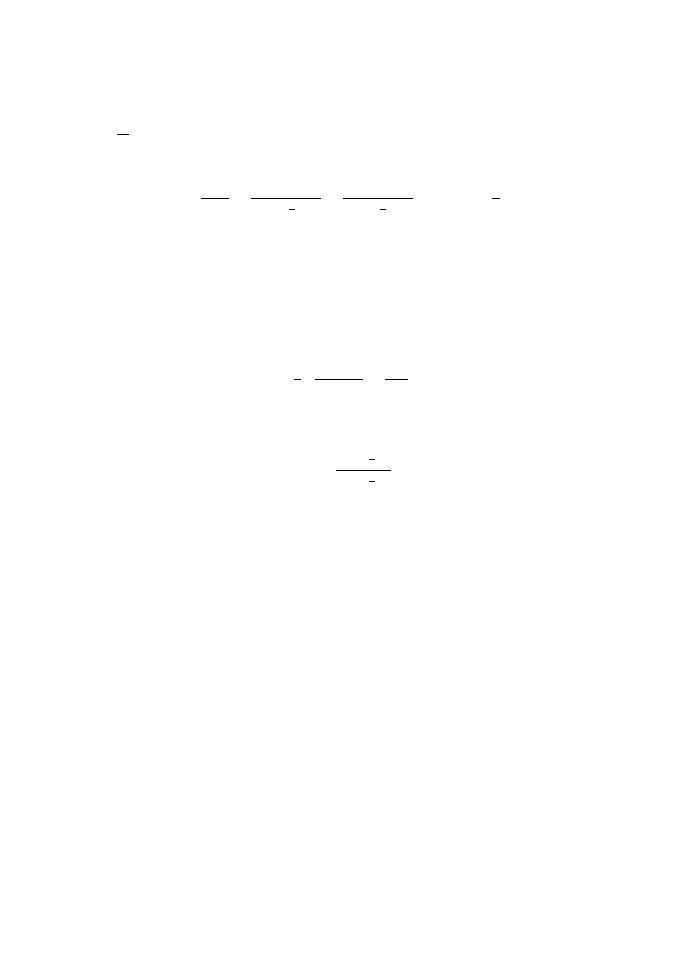
Montgomery’s pair of pants
93
In the case H =
L = 0, we can reduce (Montgomery, 2005) the planar three body orbits
with the
1
r
2
potential and equal masses to the geodesics of a metric on a four-dimensional
space (i.e., two complex dimensions, if we think of R
1,2
as complex numbers z
1,2
).
ds
2
=
1
|z
1
|
2
+
1
|z
2
+
1
2
z
1
|
2
+
1
|z
2
−
1
2
z
1
|
2
|dz
1
|
2
+
2
3
|dz
2
|
2
There is an isometry (symmetry) z
a
→ λz
a
, 0
= λ ∈ C, which combines rotations and
scaling. We can use this to remove two dimensions to get a metric on
C
ds
2
= U (z)
|dz|
2
where the effective potential
U (z) =
7
6
1
|z − 1|
2
+
1
|z|
2
+
|z|
2
is a positive function of
z =
z
2
+
1
2
z
1
z
2
−
1
2
z
1
It is singular at the points z = 0, 1,
∞, corresponding to pairwise collisions. These sin-
gular points are at an infinite distance away in this metric. (This distance has the meaning
of action. So the collisions can happen in finite time, even if the distance is infinite.) Near
each singularity the metric looks asymptotically like a cylinder: rather like a pair of pants
for a tall thin person. Thus, we get a metric that is complete on the Riemann sphere with
three points removed. Topologically, this is the same as the plane with two points removed:
C
− {0, 1}.
From Riemannian geometry (Morse theory), we know that there is a minimizing geodesic
in each homotopy class: there is an orbit that minimizes the action with a prescribed
sequence of turns around each singularity. Let A be the homotopy class of curves that wind
around 0 once in the counter-clockwise direction and B one that winds around 1. Then A
−1
and B
−1
wind around 0, 1 in the clockwise direction. Any homotopy class of closed curve
s
corresponds to a finite word made of these two letters
A
m
1
B
n
1
A
m
2
B
n
2
· · ·
or
B
n
1
A
m
1
A
m
2
B
n
2
· · ·
with non-zero m
a
, n
a
. These form a group F
2
, the free group on two generators: A and B
do not commute. Indeed they satisfy no relations among each other at all. There are an

94
The three body problem
exponentially large number of distinct words of a given length: F
2
is a hyperbolic group.
Given each such word we have a minimizing orbit that winds around 0 a certain number
m
1
times, then around 1 a certain number n
1
times then again around 0 some number m
1
times and so on.
Moreover, the curvature of the metric is negative everywhere except at two points
(Lagrange points) where it is zero. Thus the geodesics diverge from each other everywhere.
A small change in the initial conditions can make the orbit careen off in some unpre-
dictable direction, with a completely different sequence of A’s and B’s. This is chaos. The
more realistic
1
r
potential is harder to analyze, but is believed to have similar qualitative
behavior.
Problem 11.2: Find the formula [11.5] for the function U(z) by making changes
of variables
z
1
= (z
− 1)e
λ
,
z
2
=
z + 1
2
e
λ
in the metric [11.5]. Compute the curvature (Ricci scalar) in terms of derivatives
of U . Show that the curvature is zero near the apparent singularities z = 0, 1,
∞
corresponding to collisions. Find local changes of variables near these points to
show that the metric is that of a cylinder asymptotically. Plot some geodesics
of this metric by numerical calculation.
Problem 11.3: Virial Theorem Show that for a bound gravitational system
(i.e., the bodies orbit each other for ever) twice the average kinetic energy is
equal to the negative of the average potential energy. The averages are taken
over a long time along a solution:
< f >= lim
τ
→∞
1
τ
τ
0
f (
r
a
(t),
p
a
(t))dt
The key is to show that 2T + U is a total time derivative, and so has zero
average.
Problem 11.4: Research project
∗∗∗
Find the action of the minimizing geodesic
for each element of F
2
. Use this to evaluate Gutzwiller’s trace formula for ζ(s),
the sum over closed orbits. Compare with the Selberg-zeta function of Riemann
surfaces.

12
The restricted three body problem
A particular case of the three body problem is of historical importance in astronomy: when
one of the bodies is of infinitesimal mass m
3
and the other two bodies (the primaries of
masses m
1
, m
2
) are in circular orbit around their center of mass; moreover, the orbit of
the small body lies in the same plane as this circle. This is a good approximation for a
satellite moving under the influence of the Earth and the Moon; an asteroid with the Sun
and Jupiter; a particle in a ring of Saturn influenced also by one of its moons. The basic
results are due to Lagrange, but there are refinements (e.g., “halo orbits”) being discovered
even in our time.
Since the secondary has infinitesimal mass, its effect on the primaries can be ignored. Choose
a reference frame where the center of mass of the primaries is at rest at the origin. The
relative co-ordinate will describe an ellipse. We assume that the eccentricity of this orbit is
zero, a circle centered at the origin. If R is the radius (the distance between the primaries)
and Ω the angular velocity,
m
1
m
2
m
1
+ m
2
RΩ
2
=
Gm
1
m
2
R
2
, =
⇒ Ω
2
R
3
= G(m
1
+ m
2
)
This is just Kepler’s third law. The distance of the first primary from the c.m. is νR
with ν =
m
2
m
1
+m
2
. We can assume that m
1
> m
2
so that ν <
1
2
. The other primary will be
at a distance (1
− ν)R in the opposite direction. Thus the positions of the primaries are, in
Cartesian co-ordinates,
(νR cos Ωt, νR sin Ωt)
and
(
−[1 − ν]R cos Ωt, −[1 − ν]R sin Ωt)
The secondary will move in the gravitational field created by the two primaries. This field
is time dependent, with a period equal to
2π
Ω
. The Lagrangian is
L =
1
2
m
3
˙r
2
+
1
2
m
3
r
2
˙
φ
2
+ G(m
1
+ m
2
)m
3
1
− ν
ρ
1
(t)
+
ν
ρ
2
(t)

96
The restricted three body problem
where ρ
1,2
(t) are the distances to the primaries:
ρ
1
(t) =
√
r
2
+ ν
2
R
2
− 2νrR cos[φ − Ωt]
ρ
2
(t) =
√
r
2
+ (1
− ν)
2
R
2
+ 2(1
− ν)rR cos[φ − Ωt]
We can choose a unit of mass so that m
3
= 1, a unit of distance so that R = 1 and a
unit of time so that Ω = 1. Then G(m
1
+ m
2
) = 1 as well. The Lagrangian simplifies to
L =
1
2
˙r
2
+
1
2
r
2
˙
φ
2
+
1
− ν
ρ
1
(t)
+
ν
ρ
2
(t)
Since the Lagrangian is time dependent, energy is not conserved: the secondary can
extract energy from the rotation of the primaries. But we can make a transformation to a
rotating co-ordinate
χ = φ
− t
to eliminate this time dependence
L =
1
2
˙r
2
+
1
2
r
2
[ ˙
χ + 1]
2
+
1
− ν
r
1
+
ν
r
2
where
r
1
=
√
r
2
+ ν
2
− 2νr cos χ
,
r
2
=
√
r
2
+ (1
− ν)
2
+ 2(1
− ν)r cos χ
We pay a small price for this: there are terms in the Lagrangian that depend on ˙
χ linearly.
These lead to velocity dependent forces (the Coriolis force) in addition to the more familiar
centrifugal force. Nevertheless, we gain a conserved quantity, the hamiltonian.
H = ˙r
∂L
∂ ˙r
+ ˙
χ
∂L
∂ ˙
χ
− L
H =
1
2
˙r
2
+
1
2
r
2
˙
χ
2
−
r
2
2
+
1
− ν
r
1
+
ν
r
2
This is the sum of kinetic energy and a potential energy of the secondary; it is often
called the Jacobi integral. (“Integral” in an old term for a conserved quantity.) The Coriolis
force does no work, being normal to the velocity always, so it does not contribute to the
energy. It is important this is the energy measured in a non-inertial reference frame, which
is why it includes the term
∝ r
2
, the centrifugal potential.
The Lagrangian can also be written in rotating Cartesian co-ordinates
L =
1
2
˙x
2
+
1
2
˙
y
2
+ Ω [x ˙
y
− y ˙x] − V (x, y)
V (x, y) =
−
x
2
+ y
2
2
+
1
− ν
r
1
+
ν
r
2
(12.1)
r
1
=
(x
− ν)
2
+ y
2
,
r
2
=
(x + [1
− ν])
2
+ y
2

Equilibrium points
97
Exercise 12.1: Show that this leads to a hamiltonian
H =
1
2
v
2
x
+
1
2
v
2
y
+ V (x, y)
with the unusual Poisson brackets for the velocities:
{v
x
, x
} = 1 = {v
y
, y
}, {v
x
, y
} = 0 = {v
y
, x
}, {v
x
, v
y
} = −2Ω
(12.2)
The Coriolis force behaves much like a constant magnetic field normal to the
plane; we will see later that a magnetic field modifies the Poisson brackets of
velocities as well.
It is useful to express the potential energy in terms of r
1
and r
2
, eliminating r. From the
definition of r
1,2
we can verify that
[1
− ν]r
2
1
+ νr
2
2
− ν(1 − ν) = r
2
Thus
V =
−
(1
− ν)
1
r
1
+
r
2
1
2
+ ν
1
r
2
+
r
2
2
2
except for an additive constant. In studying the potential, we can use the distances r
1
and r
2
themselves as co-ordinates in the plane: the identity above shows that the potential
is separable with this choice. But beware that this system breaks down along the line
connecting the primaries. Along this line r
1
+ r
2
= 1, and so they are not independent
variables. Also, these variables cover only one half of the plane, the other half being obtained
by reflection about the line connecting the primaries.
There are points where the forces are balanced such that the secondary can be at rest. (In
the inertial frame, it will then rotate at the same rate as the primaries.)
A short exercise in calculus will show that there is a maximum of the potential when
r
1
= r
2
= 1
That is, when the thee bodies are located along the vertices of an equilateral triangle.
There are actually two such points, on either side of the primary line. They are called
Lagrange points L
4
and L
5
. There are three more equilibrium points L
1
, L
2
, L
3
that lie
along the primary line y = 0. They are not visible in terms of r
1
and r
2
because that

98
The restricted three body problem
system breaks down there. But in the Cartesian co-ordinates, it is clear by the symmetry
y
→ −y that
∂V
∂y
= 0,
if y = 0
When y = 0,
V =
−
x
2
2
+
1
− ν
|x − ν|
+
ν
|x + [1 − ν]|
This function has three extrema, L
1
, L
2
, L
3
. As functions of x these are maxima, but
are minima along y: they are saddle points of V . There are no other equilibrium points.
It is already clear that for a given H, only the region with H
− V > 0 is accessible to the
secondary particle. For small H, the curve H = V is disconnected, with regions near m
1
and m
2
and near infinity: these are the places where the potential goes to
−∞. As H grows
to the value of the potential at L
1
(the saddle point in between the two primaries), the two
regions around the primaries touch; as H grows higher, they merge into a single region. It
is only as H grows larger than the potential at L
4,5
that all of space is available for the
secondary.
For example, if a particle is to move from a point near m
1
to one near m
2
, the least
amount of energy it needs to have is the potential at the Lagrange point in between them.
The saddle point is like a mountain pass that has to be climbed to go from one deep
valley to another. This has interesting implications for space travel, many of which have
been explored in fiction. For example, in the imagination of many authors, Lagrange points
would have strategic importance (like straits that separate continents) to be guarded by star
cruisers. Belbruno, Marsden and others have scientifically sound ideas on transfer orbits of
low fuel cost. It turns out that very low cost travel is possible if we allow orbits to wind
around many times: it would take a few weeks to get to the moon instead of days as with
the more direct routes. One is reminded of the era of slow travel around the world by sailing
ships.
The second derivative of the potential
Th equilibrium points L
4
, L
5
, being at the maximum of a potential, would ordinarily be
unstable. But an amazing fact discovered by Lagrange is that the velocity dependence of
the Coriolis force can (if ν is not too close to a half) make them stable equilibria. Such a
reversal of fortune does not happen for L
1
, L
2
, L
3
: saddle points are not turned into stable
equilibria. But it has been found recently (numerically) that there are orbits near these
points, called halo orbits which do not cost much in terms of rocket fuel to maintain (see
Fig. 12.1).
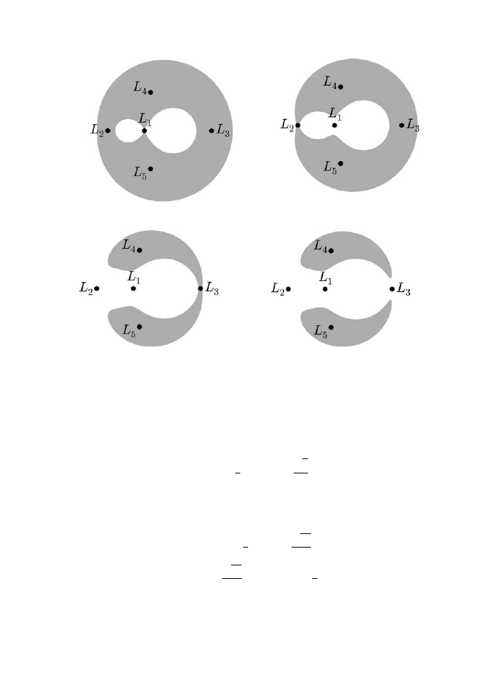
The second derivative of the potential
99
Fig. 12.1
Hill’s regions for
ν = 0.2. The orbit cannot enter the gray region, which shrinks as H
grows.
To understand the stability of L
4
and L
5
we must expand the Lagrangian to second
order around them and get an equation for small perturbations. The locations of L
4,5
are
x =
ν
−
1
2
,
y =
±
√
3
2
The second derivative of V at L
4,5
is
V
≡ K = −
⎡
⎢
⎢
⎣
3
4
±
√
27
4
[1
− 2ν]
±
√
27
4
[1
− 2ν]
9
4
⎤
⎥
⎥
⎦
Note that K < 0: both its eigenvalues are negative. On the other hand, for L
1,2,3
we
will have a diagonal matrix for K with one positive eigenvalue (along y) and one negative
eigenvalue (along x).

100
The restricted three body problem
The Lagrangian takes the form, calling the departure from equilibrium (q
1
, q
2
)
L
≈
1
2
˙
q
i
˙
q
i
−
1
2
F
ij
q
i
˙
q
j
−
1
2
K
ij
q
i
q
j
where
F = 2
0
−1
1 0
comes from the Coriolis force. For small q, the equations of motion become
¨
q + F ˙
q + Kq = 0
We seek solutions of the form
q(t) = e
iωt
A
for some constant vector and frequency ω. Real values of ω would describe stable
perturbations. The eigenvalue equation is somewhat unusual
[
−ω
2
+ F iω + K]A = 0
in that it involves both ω and ω
2
. Thus the characteristic equation is
det[
−ω
2
+ F iω + K] = 0
Or
det
K
11
− ω
2
K
12
− 2iω
K
12
+ 2iω K
22
− ω
2
= 0
which becomes
ω
4
− [4 + trK]ω
2
+ det K = 0
There are two roots for ω
2
.
(ω
2
− λ
1
)(ω
2
− λ
2
) = 0
The condition for stability is that both roots must be real and positive. This is equivalent
to requiring that the discriminant is positive and also that λ
1
λ
2
> 0, λ
1
+ λ
2
> 0. Thus
[trK + 4]
2
− 4 det K > 0, det K > 0, trK + 4 > 0

Stability theory
101
So,
det K > 0,
trK + 4 > 2
√
det K
The first condition cannot be satisfied by a saddle point of V : the eigenvalues of K has
opposite signs. So L
1,2,3
are unstable equilibria. It can be satisfied by a minimum, for which
K > 0.
But surprisingly, it can also be satisfied by a maximum of a potential. For L
4,5
trK =
−3, det K =
27
4
ν(1
− ν)
Since we chose ν <
1
2
, we see that det K > 0.
The second condition of (12.7) becomes
27ν(1
− ν) < 1
In other words,
ν <
1
2
1
−
1
−
4
27
≈ 0.03852
(Recall that we chose ν <
1
2
; by calling m
1
the mass of the larger primary.) Thus we get
stability if the masses of the two primaries are sufficiently different from each other. In this
case, the frequencies are
ω =
1
±
1
− 27ν(1 − ν)
2
in units of Ω.
When ν
1, one of these frequencies will be very small, meaning that the orbit is nearly
synchronous with the primaries.
For the Sun–Jupiter system, ν = 9.5388
× 10
−4
so the Lagrange points are stable. The
periods of libration (the small oscillations around the equilibrium) follow from the orbital
period of Jupiter (11.86 years): 147.54 years or 11.9 years. For the Earth–Moon system
ν =
1
81
is still small enough for stability. The orbital period being 27.32 days, we have
libration periods of 90.8 days and 28.6 days.
Lagrange discovered something even more astonishing: the equilateral triangle is a sta-
ble exact solution for the full three body problem, not assuming one of the bodies to be
infinitesimally small. He thought that these special solutions were artificial and that they
would never be realized in nature. But we now know that there are asteroids (Trojan aster-
oids) that form an equilateral triangle with the Sun and Jupiter. The Earth also has such
a co-traveller at its Lagrange point with the Sun.

102
The restricted three body problem
Problem 12.2: What is the minimum energy per unit mass needed to travel
from a near-Earth orbit (100 km from the Earth’s surface) to the surface of the
Moon?
Problem 12.3: Suppose that a particle in libration around a Lagrange point is
subject to a frictional force proportional to its velocity. Will it move closer to or
farther away from the Lagrange point? Find its orbit in the linear approximation
in the displacement. Assume that the coefficient of friction is small.
Problem 12.4: Suppose that the orbit of the primaries have a small eccentric-
ity . To the leading order in , find the correction to the equation of motion of
the secondary.
Problem 12.5: Without assuming that the masses are very different from each
other, show that there is a solution of the three body problem where the bodies
are equidistant from each other.

The force on a charged particle in a static magnetic field is normal to its velocity. So it does
no work on the particle. The total energy of the particle is not affected by the magnetic
field. The hamiltonian as a function of position and velocities does not involve the magnetic
field. Can Hamiltonian mechanics still be used to describe such systems? If so, where does
the information about the magnetic field go in? It turns out that the magnetic field modifies
the Poisson brackets and not the hamiltonian.
d
r
dt
=
v,
d
d
[m
v] = ev × B
Or in terms of components
m
dx
i
dt
= v
i
,
d
dt
[mv
i
] = e
ijk
v
j
B
k
Here
ijk
is completely antisymmetric and
123
= 1
Let us assume that the magnetic field does not depend on time, only on the position;
otherwise, we cannot ignore the electric field.
The energy (hamiltonian) is just
H =
1
2
mv
i
v
i
We want however,
H, x
i
= v
i
,
{H, v
i
} =
e
m
ijk
v
j
B
k

104
Magnetic fields
The first is satisfied if
p
i
, x
j
=
1
m
δ
ij
which is the usual relation following from canonical relations between position and
momentum. So we want
1
2
mv
j
v
j
, v
i
=
e
m
ijk
v
j
B
k
Using the Leibnitz rule this becomes
v
j
v
j
, v
i
=
e
m
2
ijk
v
j
B
k
It is therefore sufficient that
{v
j
, v
i
} =
e
m
2
ijk
B
k
This is not what follows from canonical relations; the different components of momentum
would commute then. To make this distinction clear, let us denote momentum by
π
i
= mv
i
Then:
{x
i
, x
j
} = 0,
π
i
, x
j
= δ
ij
,
{π
i
, π
i
} = −eF
ij
where
F
ij
=
ijk
B
k
The brackets are antisymmetric. The Jacobi identity is automatic for all triples of
variables except one:
{{π
i
, π
j
} , π
k
} = −e {F
ij
, mv
k
}
= e∂
k
F
ij
Taking the cyclic sum, we get
∂
i
F
jk
+ ∂
j
F
ki
+ ∂
k
F
ij
= 0
If you work out in components you will see that this is the condition
∇ · B = 0

The Lagrangian
105
which is one of Maxwell’s equations. Thus the Jacobi identity is satisfied as long as Maxwell’s
equation is satisfied.
If we have an electrostatic as well as a magnetic field the hamiltonian will be
H =
π
i
π
i
2m
+ eV
again with the commutation relations above.
It is possible to bring the commutation relations back to the standard form
{x
i
, x
j
} = 0,
p
i
, x
j
= δ
ij
,
{p
i
, p
i
} = 0
in those cases where the magnetic field is a curl. Recall that locally, every field satisfying
∇ · B = 0
is of the form
B = ∇ × A
for some vector field
A. This is not unique: a change (gauge transformation)
A → A + ∇Λ
leaves
B unchanged. Now if we define
π
i
= p
i
− eA
i
then the canonical relations imply the relations for π
i
.
This suggests that we can find a Lagrangian in terms of A
i
. We need
p
i
=
∂L
∂ ˙x
i
or
∂L
∂ ˙x
i
= m ˙x
i
+ eA
i

106
Magnetic fields
Thus we propose
L =
1
2
m ˙x
i
˙x
i
+ eA
i
˙x
i
− eV
as the Lagrangian for a particle in an electromagnetic field.
Exercise 13.1: Show that the Lorentz force equations follows from this
Lagrangian.
An important principle of electromagnetism is that the equations of motion
should be invariant under gauge transformations A
i
→ A
i
+ ∂
i
Λ. Under this
change the action changes to
S =
t
2
t
1
Ldt
→ S +
t
2
t
1
e ˙x
i
∂
i
Λdt
The extra term is a total derivative, hence only depends on endpoints:
t
2
t
1
e
dΛ
dt
dt = e [Λ(x(t
2
))
− Λ(x(t
1
))]
Since we hold the endpoints fixed during a variation, this will not affect the
equations of motion.
Recall that the electric field of a point particle satisfies
∇ · E = 0
everywhere but at its location. Can there be point particles that can serve as sources of
magnetic fields in the same way? None have been discovered to date: only magnetic dipoles
have been found, a combination of north and south poles. Dirac discovered that the existence
of even one such magnetic monopole somewhere in the universe would explain a remarkable
fact about nature: that electric charges appear as multiples of a fundamental unit of charge.
To understand this let us study the dynamics of an electrically charged particle in the field
of a magnetic monopole, an analysis due to M. N. Saha.
d
r
dt
=
v,
d
d
[m
v] = egv ×
r
r
3
where r is the strength of the magnetic monopole. The problem has spherical symmetry, so
we should expect angular momentum to be conserved. But we can check that
d
dt
[
r × mv] = egr ×
v ×
r
r
3
is not zero. What is going on? Now, recall that identity
d
dt
r
r
=
v
r
−
r
r
2
˙r

The magnetic monopole
∗
107
But
˙r =
1
2r
d
dt
[
r · r]
=
1
r
r · v
So
d
dt
r
r
=
r
2
v − r(v · r)
r
3
or
d
dt
r
r
=
1
r
3
r × [v × r]
Thus we get a new conservation law
d
dt
r × mv − eg
r
r
= 0
The conserved angular momentum is the sum of the orbital angular momentum and
a vector pointed along the line connecting the charge and the monopole. This can be
understood as the angular momentum contained in the electromagnetic field. When an
electric and a magnetic field exist together, they carry not only energy but also momentum
and angular momentum. If you integrate the angular momentum density over all of space
in the situation above, you will get exactly the extra term
J = r × mv − eg
r
r
which is a fixed vector in space. The orbit does not lie in the plane normal to to
J. Instead
it lies on a cone, whose axis is along
J. The angle α of this cone is given by
J cos α =
J ·
r
r
=
−eg
13.5.1
Quantization of electric charge
If we quantize this system, we know that an eigenvalue of J
3
is an integer or half-integer
multiple of
and that the eigenvalues of J
2
are j(j + 1) where j is also such a multiple. On
the other hand,
L = r × mv is also quantized in the same way. It follows that the vector
eg
r
r
must have a magnitude which is a multiple of
eg = n
, n =
1
2
, 1,
3
2
, 2,
· · ·
Thus, if there is even one magnetic monopole somewhere in the universe, electric charge
has to be quantized in multiples of
2g
. We do see that electric charge is quantized this way,
the basic unit being the magnitude of the charge of the electron. We do not yet know if the
reason for this is the existence of a magnetic monopole.

108
Magnetic fields
A static electromagnetic field can be used to trap charged particles. You can bottle up anti-
matter this way; or use it to hold an electron or ion in place to make precise measurements
on it.
It is not possible for a static electric field by itself to provide a stable equilibrium
point: the potential must satisfy the Laplace equation
∇
2
V = 0. So at any point the sum
of the eigenvalues of the Hessian matrix V
(second derivatives) must vanish. At a stable
minimum they would all have to be positive. It is possible to have one negative and two
positive eigenvalues. This is true for example for a quadrupole field
V (x) =
k
2
2x
2
3
− x
2
1
− x
2
2
Such a field can be created by using two electrically charged conducting plates shaped
like the sheets of a hyperboloid:
x
2
1
+ x
2
2
− 2x
2
3
= constant
So, the motion in the x
1
−x
2
plane is unstable but that along the x
3
axis is stable. Now
we can put a constant magnetic field pointed along the x
3
-axis. If it is strong enough, we
get a stable equilibrium point at the origin. This stabilization of a maximum by velocity-
dependent forces is the phenomenon we saw first at the Lagrange points of the three body
problem.
Look at the equation of motion of a particle in a constant magnetic field and an
electrostatic potential that is a quadratic function of position, V (x) =
1
2
x
T
Kx.
¨
q + F ˙
q +
e
m
Kq = 0
Here F is an antisymmetric matrix proportional to the magnetic field. For a field of
magnitude B along the x
3
-axis
F =
e
m
⎛
⎝
0
B 0
−B 0 0
0
0 0
⎞
⎠
If we assume the ansatz
q = Ae
iωt
the equation becomes
−ω
2
+ iωF +
e
m
K
A = 0
which gives the characteristic equation
det
−ω
2
+ iωF +
e
m
K
= 0

The Penning trap
109
If the magnetic field is along the third axis and if the other matrix has the form
K =
⎛
⎝
k
1
0
0
0 k
2
0
0
0 k
3
⎞
⎠
this equation factorizes
(
−ω
2
+ k
3
) det
⎡
⎢
⎢
⎣
e
m
k
1
− ω
2
iω
eB
m
−iω
eB
m
e
m
k
2
− ω
2
⎤
⎥
⎥
⎦ = 0
The condition for stability is that all roots for ω
2
are positive. One of the roots is k
3
, so
it must be positive. It is now enough that the discriminant as well as the sum and product
of the other two roots are positive. This amounts to
k
3
> 0,
k
1
k
2
> 0,
eB
2
m
> 2
k
1
k
2
− (k
1
+ k
2
)
The physical meaning is that the electrostatic potential stabilizes the motion in the
x
3
-direction. Although the electric field pushes the particle away from the origin, the
magnetic force pushes it back in.
A collection of particles moving in such a trap will have frequencies dependent on the
ratios
e
m
. These can be measured by Fourier transforming the electric current they induce
on a probe. Thus we can measure the ratios
e
m
, a technique called Fourier transform mass
spectrometry.
Problem 13.2: Find the libration frequencies of a charged particle in a Penning
trap.
Problem 13.3: Verify that J of a charged particle in the field of a magnetic
monopole satisfies the commutation relations of angular momentum
{J
i
, J
j
} =
ijk
J
k
Does orbital angular momentum
r × mv satisfy these relations?
Problem 13.4: Determine the orbit of a charged particle moving in the field
of a fixed magnetic monopole. Exploit the conservation of energy and angular
momentum. You should find that the orbit lies on a cone whose axis is along
J.

This page intentionally left blank

14
Poisson and symplectic manifolds
Classical mechanics is not just old mechanics. It is the approximation to mechanics in which
the quantum effects are small. By taking limits of quantum systems, we sometimes discover
new classical systems that were unknown to Hamilton or Euler. A good example of this is
the concept of spin. It used to be thought that the only way a particle can have angular
momentum is if it moves:
L = r × m˙r. But we saw a counter-example in the last chapter:
a charge and a magnetic monopole can have angular momentum even if they are at rest,
because the electric and magnetic fields carry angular momentum. But this is an exotic
example, one that has not yet been realized experimentally.
But almost every particle (the electron, the proton, the neutron etc.) of which ordinary
matter is made of carries spin: it has angular momentum even when it is at rest. For
each particle this is small (of order
), so it is outside of the domain of classical physics.
But a large number of such particles can act in unison to create a spin big enough to be
treated classically. An example of this is nuclear magnetic resonance, where a large number
(N
≈ 10
23
) of atomic nuclei at rest orient their spins in the same direction. This happens
because they carry a magnetic moment parallel to the spin, and if you apply a magnetic
field, the minimum energy configuration is to have the spins line up. The time evolution of
this spin can be described classically, as the spin is large compared to
.
There are some unusual things about this system though: its phase space has finite
area. It is a sphere. So it will not be possible to separate its co-ordinates into conjugate
variables globally. This does not matter: we still have a Poisson bracket and can still derive
a hamiltonian formalism.
Poisson brackets on the sphere
The essential symmetry of the sphere is under rotations. Recall the commutation relations
of infinitesimal rotations
{S
1
, S
2
} = S
3
,
{S
2
, S
3
} = S
1
,
{S
3
, S
1
} = S
1
Or, in the index notation
{S
i
, S
j
} =
ijk
S
k

112
Poisson and symplectic manifolds
In particular, the Jacobi identity is satisfied. Note that
S · S commutes with every
component. So we can impose the condition that it is a constant
S
2
=
S|S · S = s
2
This way, we get a Poisson bracket of a pair of functions on the sphere
{F, G} =
ijk
S
i
∂F
∂S
j
×
∂G
∂S
k
Or equivalently,
{F, G} = S ·
∂F
∂
S
×
∂G
∂
S
If you find this formulation too abstract, you can use spherical polar co-ordinates
S
1
= s sin θ cos φ,
S
2
= s sin θ sin φ,
s
3
= s cos θ
so that the Poisson bracket can be written as
{φ, cos θ} = 1
In some sense φ and cos θ are canonically conjugate variables. But this interpretation is not
entirely right: unlike the usual canonical variables, these are bounded. Also, they are not
globally well-defined co-ordinates on the sphere. For example, φ jumps by 2π when we make
a complete rotation. This won’t matter as long as only local properties in the neighborhood
of some point are studied. But global questions (such as quantization or chaos) are best
studied in a co-ordinate independent way.
Consider a large number of identical particles, each with a magnetic moment proportional
to its spin. Then the total magnetic moment will also be proportional to spin:
M = gS
In the presence of an external magnetic field the energy of this system will be
H = g
B · S
The time evolution of the spin is then given by Hamilton’s equations
d
S
dt
= g
B × S

Poisson manifolds
113
The solution is easy to find: the spin precesses at a constant rate around the magnetic field.
The frequency of this precession is
ω = g
|B|
If the initial direction of the magnetic moment was parallel to the magnetic field (minimum
energy) or antiparallel (maximum of energy) the spin will not precess. Otherwise it will
precess in a circle determined by the energy. Suppose that all the magnetic moments are in
the lowest energy state, aligned with the magnetic field. If we now send in an electromagnetic
wave at just this frequency, the spins will absorb the energy and start to precess. This is
the phenomenon of nuclear magnetic resonance (NMR). This absorption can be detected
and used to measure the density of the spins. If we create a slowly varying magnetic field
(instead of a constant one as we have assumed so far) the resonant frequency will depend on
position. By measuring the amount of electromagnetic energy absorbed at each frequency,
we can deduce the density of nuclei at each position. This is the technique of NMR imaging.
Thus we see that hamiltonian mechanics makes sense even when it is not possible to find
global canonical co-ordinates. All we need is a Poisson bracket among functions that satisfies
the following axioms:
{F, aG + bH} = a{F, G} + b{F, H}, a, b ∈ R, linearity
{F, GH} = {F, G}H + F {G, H}, Leibnitz identity
{F, G} = −{G, F }, antisymmetry
{{F, G}, H} + {{G, H}, F } + {{H, F }, G} = 0, Jacobi identity
The first two say that there is a second rank contra-variant tensor r such that
{F, G} = r
ij
∂
i
F ∂
j
G
This tensor must be antisymmetric
r
ij
=
−r
ji
The Jacobi identity is then a condition on its derivatives
r
im
∂
m
r
jk
+ r
jm
∂
m
r
ki
+ r
km
∂
m
r
ij
= 0
A manifold along with such an tensor on it is called a Poisson manifold. The sphere is an
example, as saw above.

114
Poisson and symplectic manifolds
Example 14.1: Three-dimensional Euclidean space R
3
is a Poisson manifold
with r
ij
=
ijk
x
k
. Verify the Jacobi identity.
A particularly interesting kind of Poisson manifold is an irreducible one: the
only central functions (i.e., those that commute with all other functions) are
constants:
{F, G} = 0, ∀G =⇒ ∂
i
F = 0
R
3
is not irreducible:
|x|
2
= x
i
x
i
commutes with everything. By setting it equal
to a constant, we get a sphere which is irreducible. More generally, a Poisson
manifold can be (locally) decomposed as a union of irreducibles, which are the
submanifolds on which the central functions are held constant.
On an irreducible Poisson manifold, r
ij
has an inverse
r
ij
ω
jk
= δ
i
k
In terms of this inverse, the Jacobi identity is a linear equation:
∂
i
ω
jk
+ ∂
j
ω
ki
+ ∂
k
ω
ij
= 0
This condition has an elegant meaning in differential geometry: ω = ω
ij
dx
i
∧ dx
j
is a closed differential form, dω = 0. A closed invertible differential form is called
a symplectic form; thus irreducible Poisson manifolds are symplectic manifolds.
The sphere is the simplest example.
Exercise 14.1: Show that all symplectic manifolds are even-dimensional. (Can
an antisymmetric matrix of odd dimension have non-zero determinant?)
There are local co-ordinates (q, p) on a symplectic manifold such that ω is a
constant,
ω = dq
i
∧ dp
i
In these coordinates the Poisson bracket reduces to the form
{F, G} =
i
∂F
∂p
i
∂G
∂q
i
−
∂F
∂q
i
∂G
∂p
i
we had earlier. But the co-ordinate independent point of view is more natural
and allows for the treatment of many more physical systems (such as spin).
The determinant of an antisymmetric matrix of even dimension is the square of a polynomial
in its matrix elements. This polynomial is called the Pfaffian. The Pfaffian of the symplectic
form is density in the phase space. As canonical transformations leave the symplectic form
unchanged, they leave this density unchanged as well. In the simplest case ω = dq
i
∧ dp
i
the density is just dqdp. That the volume element in phase space, dqdp, is invariant under
time evolution is an ancient result, known as Liouville’s theorem.

Liouville’s theorem
115
Problem 14.2: In a ferromagnetic material, each atom has an unpaired elec-
tron which carries a magnetic moment and
2
of spin. What is the spin of a
ferromagnet consisting of one kilogram of iron, in which about a tenth of the
unpaired electrons are lined up?
Problem 14.3: A Grassmannian is a generalization of the sphere. It may be
thought of as the set of all M
× M hermitian matrices equal to their own squares
(orthogonal projectors). Such matrices have eigenvalues 1 or 0. The number of
non-zero eigenvalues is called the rank.
Gr
m
(M ) =
{P |P
2
= P, P
†
= P, tr P = m
}
Show that: The case M = 2, m = 1 corresponds to the sphere. ω = tr P dP
∧ dP is
a symplectic form on the Gr
m
(M ). The Poisson brackets of the matrix elements
of P are
{P
i
j
, P
k
l
} = δ
k
j
P
i
l
− δ
i
l
P
k
j

This page intentionally left blank

Is the flow of time continuous? Or is it discrete, like sand in an hourglass? As far as
we know now, it is continuous. Yet, it is convenient in many situations to think of it
as discrete. For example, in solving a differential equation numerically, it is convenient
to calculate the finite change over a small time interval and iterate this process. It is
important that we retain the symmetries and conservation laws of the differential equation
in making this discrete approximation. In particular, each time step must be a canonical
(also called symplectic) transformation. Such symplectic integrators are commonly used to
solve problems in celestial mechanics.
Another reason to study discrete time evolution is more conceptual. It goes back to
Poincar´
e’s pioneering study of chaos. Suppose that we have a system with several degrees
of freedom. We can try to get a partial understanding by projecting to one degree of freedom
(say (p
1
, q
1
)). That is, we look only at initial conditions where the degrees of freedom are
fixed at some values (say (p
i
, q
i
) = 0 for i > 1). Then we let the system evolve in the full
phase space and ask when it will return to this subspace (i.e., what is the next value of
(p
1
, q
1
) for which (p
i
, q
i
) = 0 for i > 1?). This gives a canonical transformation (called the
Poincar´
e map) of the plane (p
1
, q
1
) to itself. We can then iterate this map to get an orbit,
an infinite sequence of points in the plane. In simple cases (like the harmonic oscillator),
this orbit will be periodic. If the system is chaotic, the orbit will wander all over the plane,
and it is interesting to ask for the density of its distribution: how many points in the orbit
are there in some given area? This distribution often has an interesting fractal structure:
there are islands that contain points in the orbit surrounded by regions that do not contain
any. But if we were to magnify these islands, we will see that they contain other islands
surrounded by empty regions and so on to the smallest scales.
First order symplectic integrators
Symplectic transformation is just another name for a canonical transformation, i.e., a trans-
formation that preserves the Poisson brackets. In many cases of physical interest, the
hamiltonian of a mechanical system is of the form
H = A + B
where the dynamics of A and B are separately are easy to solve. For example, if the
hamiltonian is
H = T (p) + V (q)
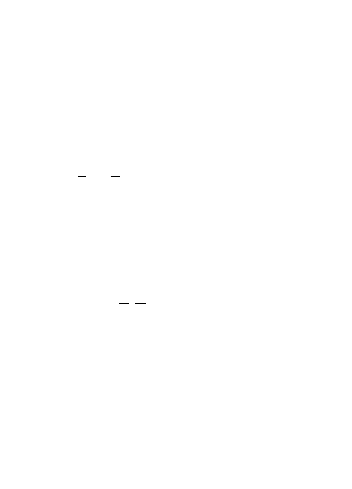
118
Discrete time
with a kinetic energy T that depends on momentum variables alone and a potential
energy V that depends on position alone, it is easy to solve the equations for each separately.
The problem is, of course, that these two canonical transformations do not commute. So
we cannot solve the dynamics of H by combining them.
But the commutator of these transformations is of order t
1
t
2
. Thus for small time inter-
vals it is small, and it might be a good approximation to ignore the lack of commutativity.
This gives a first order approximation. If we split the time into small enough intervals,
the iteration of this naive approximation might be good enough. We then iterate this time
evolution to get an approximation to the orbit. Later we will see how to improve on this
by including the effects of the commutator to the next order.
If we perform the above two canonical transformations consecutively, choosing equal
time steps , we get the discrete time evolution
p
i
= p
i
− V
i
(q),
q
i
= q
i
+ T
i
(p
)
where V
i
=
∂V
∂q
i
, T
i
=
∂T
∂p
i
. We transform p first then q because usually it leads to simpler
formulas. (See the example.) In many cases this simple “first order symplectic integrator”
already gives a good numerical integration scheme.
Example 15.1: Consider the example of the simple pendulum T =
p
2
2
, V =
ω
2
[1
− cos q] . If we perform the above two canonical transformations consecu-
tively, choosing equal time steps , we get the discrete time evolution
p
= p
− ω
2
sin q,
q
= q + p
Equivalently,
p
= p
− ω
2
sin q,
q
= q + p
−
2
ω
2
sin q
This is a canonical transformation:
det
⎡
⎢
⎢
⎣
∂p
∂p
∂p
∂q
∂q
∂p
∂q
∂q
⎤
⎥
⎥
⎦ = det
1
−ω
2
cos q
1
−
2
ω
2
cos q
= 1
Note that this determinant is one exactly, not just to second order in .
Iterating this map we get a discrete approximation to the time evolution of
the pendulum. It gives a nice periodic orbit as we expect for the pendulum (see
Fig. 15.1).
Notice that if we had made another discrete approximation (which attempts
to do the T and V transformations together) we would not have obtained a
canonical transformation:
p
= p
− ω
2
sin q,
q
= q + p
det
⎡
⎢
⎢
⎣
∂p
∂p
∂p
∂q
∂q
∂p
∂q
∂q
⎤
⎥
⎥
⎦ = det
1
−ω
2
cos q
1
= 1
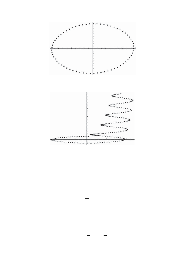
Second order symplectic integrator
119
0.5
–0.5
–1.0
–1.0
–0.5
0.5
1.0
1.0
Fig. 15.1
Symplectic integration of the pendulum.
5
10
15
20
25
30
2
1
–1
Fig. 15.2
Non-symplectic integration of the pendulum.
The orbit of this map goes wild, not respecting conservation of energy or of
area (see Fig. 15.2).
Second order symplectic integrator
Suppose we are solving a linear system of differential equations
dx
dt
= Ax
for some constant matrix A. The solution is
x(t) = e
tA
x
0
where the exponential of a matrix is defined by the series
e
tA
= 1 + tA +
1
2!
t
2
A
2
+
1
3!
t
3
A
3
+
· · ·
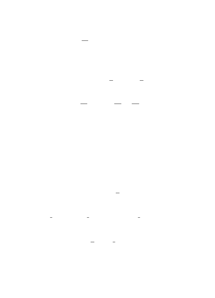
120
Discrete time
Solving non-linear differential equations
dx
i
dt
= A
i
(x),
x
i
(0) = x
i
0
is the same idea, except that the matrix is replaced by a vector field whose components
can depend on x. The solution can be thought of still as an exponential of the vector field,
defined by a similar power series. For example, the change of a function under time evolution
has the Taylor series expansion
f (x(t)) = f (x
0
) + tAf (x
0
) +
1
2!
t
2
A
2
f (x
0
) +
1
3!
t
3
A
3
f (x
0
)
Here
Af = A
i
∂f
∂x
i
,
A
2
f = A
i
∂
∂x
i
A
j
∂f
∂x
j
,
· · ·
Now, just as for matrices,
e
A
+B
= e
A
e
B
in general, because A and B may not commute. Up to second order in t we can ignore this
effect
e
t
(A+B)
= e
tA
e
tB
1 + O(t
2
)
The first order symplectic integrator we described earlier is based on this. There is
a way to correct for the commutator, called the Baker–Campbell–Hausdorff formula (or
Poincar´
e–Birkhoff–Witt lemma). To second order, it gives
Lemma 15.1:
e
tA
e
tB
= exp
tA + tB +
t
2
2
[A, B] + O(t
3
)
Proof: Expand the LHS to second order
1 + tA +
1
2
t
2
A
2
1 + tB +
1
2
t
2
B
2
= 1 + tA + tB +
1
2
t
2
(A
2
+ B
2
) + t
2
AB + O(t
3
)
The RHS to the second order is
1 + tA + tB +
t
2
2
[A, B] +
1
2
t
2
(A + B)
2
+ O(t
3
)
They agree because
A
2
+ B
2
+ 2AB = (A + B)
2
+ [A, B]
It is also possible to determine higher order corrections in the same way.

Chaos with one degree of freedom
121
Proposition 15.1: We can avoid commutators by a more symmetric
factorization
e
t
(A+B)
= e
1
2
tA
e
tB
e
1
2
tA
1 + O(t
3
)
Proof:
e
1
2
tA
e
tB
e
1
2
tA
= e
1
2
tA
e
t
2
B
e
t
2
B
e
1
2
tA
and use the BCH formula to combine the first pair and the second pair:
e
1
2
tA
e
tB
e
1
2
tA
= e
t
2
A
+
t
2
B
+
t2
8
[A,B]+···
e
t
2
A
+
t
2
B
−
t2
8
[A,B]+. . .
and then again combine the last two exponentials. All the second order terms
in t cancel out.
In our case, A and B will be generators of canonical transformations whose Hamilton’s
equations are easy to solve (i.e., e
tA
and e
tB
are known). We can then find an approximation
for the solution of Hamilton’s equations for A + B. As an example, if
H(q, p) = T (p) + V (q)
we can deduce a second order symplectic integrator (choosing A = V, B = T ). The effect of
e
2
V
is to leave q unchanged and to transform p to an intermediate variable
z
i
= p
i
−
1
2
V
i
(q)
(15.1)
where V
i
=
∂V
∂q
i
. Then we apply e
T
, which leaves p unchanged and transforms q to
q
i
= q
i
+ T
i
(z)
(15.2)
with T
i
=
∂T
∂p
i
. Finally we apply e
2
V
again to get
p
i
= z
i
−
1
2
V
i
(q
i
)
(15.3)
The formulas (15.1, 15.2, 15.3) together implement a second order symplectic integrator.
See Yoshida (1990) for higher orders.
Chaos with one degree of freedom
A Hamiltonian system with a time independent hamiltonian always has at least one con-
served quantity: the hamiltonian itself. Thus we expect all such systems with one degree
of freedom to be integrable. But if the hamiltonian is time dependent this is not the case
anymore. For example, if the hamiltonian is a periodic function of time, in each period the
system will evolve by a canonical transformation. Iterating this we will get an orbit of a
symplectic map which can often be chaotic. G. D. Birkhoff (1922) made a pioneering study
of this situation.
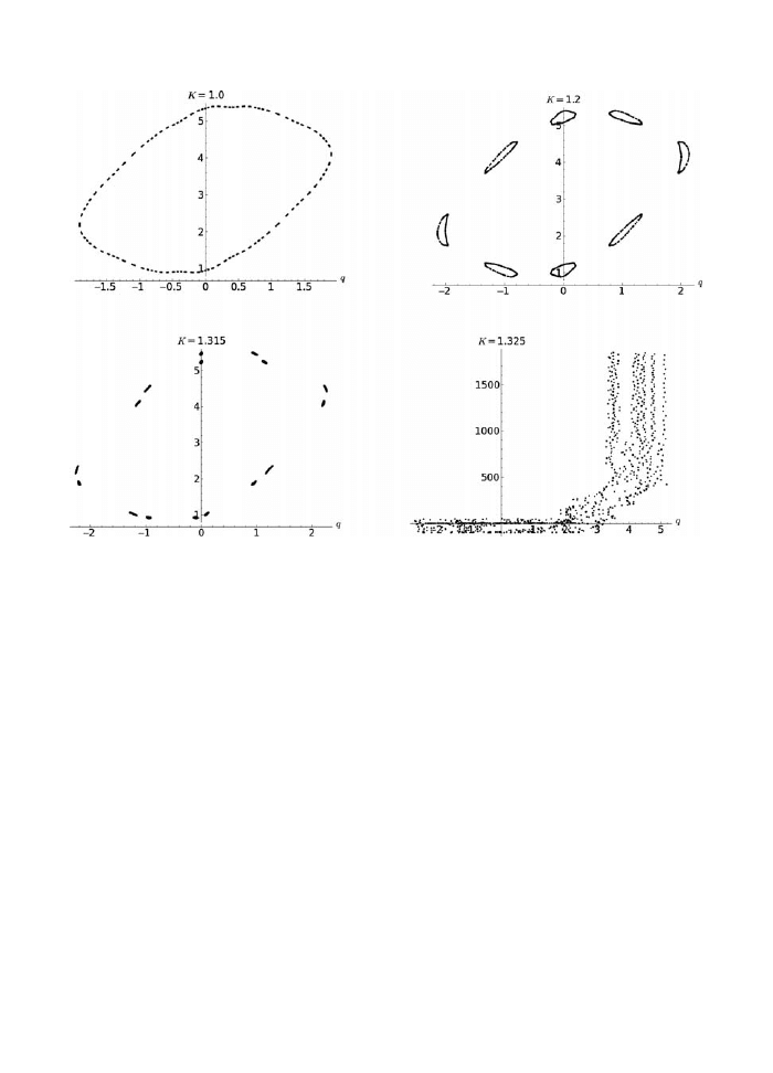
122
Discrete time
Fig. 15.3
The Chirikov standard map for the initial point
p = 0.1, q = 1 and various values of K.
Example 15.2: The Chirikov standard map is
p
n
+1
= p
n
+ K sin q
n
,
q
n
+1
= q
n
+ p
n
+1
This can be thought of as a discrete approximation to the pendulum when K
is small (see the previous example): we choose units of time so that each step is
one = 1 and put K =
−ω
2
.
But for K that is not small, it is an interesting dynamical system in its own right, iterat-
ing a canonical transformation. Although the evolution of the pendulum itself is integrable,
this discrete evolution can be chaotic when K is not small. Look at the plots of the orbits of
the same initial point (p, q) = (0.1, 1) for various values of K. Thus we see that iterations of
a canonical transformation can have quite unpredictable behavior even with just one degree
of freedom.
Birkhoff’s idea in the above-mentioned paper is to attempt to construct a conserved
quantity (hamiltonian). If the time variable were continuous this would be easy. He does an
analytic continuation of the discrete variable n and works backward to get a hamiltonian.
This continuation is done using an asymptotic series. So the hamiltonian obtained this way
is also an asymptotic series. If this series were to converge, the discrete evolution would
not be chaotic. But for most initial conditions the series is only asymptotic: the lack of

Chaos with one degree of freedom
123
convergence is due to resonances. So we will find that there are regions in the phase space
where the system behaves chaotically, interlaced with other regions where it is predictable.
A far-reaching extension of this idea was developed by Kolmogorov, Arnold and Moser
(KAM). This KAM theorem is the foundation of the modern theory of chaos in Hamiltonian
systems.
Problem 15.1: Plot the orbits of the non-symplectic integrator of the
pendulum
p
= p
− ω
2
sin q,
q
= q + p
Compare with the first order symplectic integrator
p
= p
− ω
2
sin q,
q
= q + p
Problem 15.2: Write a program (in MatLab, Mathematica, Maple or Sage)
that iterates the Chirikov standard map. Use it to plot the orbit for various
values of K.
Problem 15.3: Write a symplectic integrator for the circular restricted three
body problem. It is best to use H
0
=
1
2
(v
2
x
+ v
2
y
) with Poisson brackets as in
(12.2) and potential V as in (12.1). Plot some orbits and see that they lie
within the corresponding Hill’s region.
Problem 15.4: Arnold’s cat map Even the iteration of a linear canonical
transformation can lead to chaos, if the phase space has a periodicity that is
incommensurate with it. An example is the map
x
y
=
2 1
1 1
x
y
mod 1
Verify that this is indeed a canonical transformation, i.e., that the Jacobian is
unity. The origin is a fixed point. What are the stable
1
and unstable directions?
When is the orbit of a point periodic? Is there an orbit that is dense? Is the map
ergodic? Arnold illustrated the chaos by showing what happens to the picture
of a cat under repeated applications of this map.
1
Some of these terms are explained in later chapters. Come back to this project after you have read
them.

This page intentionally left blank

16
Dynamics in one real variable
It became clear towards the end of the nineteenth century that most systems are not
integrable: we will never get a solution in terms of simple functions (trigonometric, elliptic,
Painlev´
e etc.) The focus now shifts to studying statistical properties, such as averages over
long time. And to universal properties, which are independent of the details of the dynamics.
It is useful to study the simplest case of dynamics, the iterations of a function of a single
real variable, which maps the interval [0, 1] to itself. Even a simple function like μx(1
− x)
(for a constant μ) leads to chaotic behavior. Only since the advent of digital computers
has it become possible to understand this in some detail. But it is not the people who had
the biggest or fastest computers that made the most important advances: using a hand-
held calculator to do numerical experiments pointed Feigenbaum to patterns which led to
a beautiful general theory. The best computer is still the one between your ears.
See Strogarz (2001) for more.
A map is just another word for a function f : X
→ X that takes some set to itself. Since
the domain and range are the same, we can iterate this: given an initial point x
0
∈ X we
can define an infinite sequence
x
0
, x
1
= f (x
0
), x
2
= f (x
1
),
· · ·
i.e.,
x
n
+1
= f (x
n
)
This is an orbit of f . A fixed point of f is a point that is mapped to itself:
f (x) = x.
The orbit of a fixed point is really boring x, x, x,
· · · .
A periodic orbit satisfies
x
n
+k
= x
n
for some k. The smallest number for which this is true is called its period. For example, if
the orbit of some point is periodic with period two, it will look like
x
0
, x
1
, x
0
, x
1
, x
0
, x
1
,
· · · , x
0
= x
1

126
Dynamics in one real variable
Given a function we can define its iterates
f
2
(x) = f (f (x)),
f
3
(x) = f (f (f (x))),
· · ·
A moment’s thought will show that a fixed point of one of the iterates f
k
(x) is the same
thing as a periodic orbit of f (x). For example, if x
0
is not a fixed point of f (x) but is one
for f
2
, then its orbit under f is periodic with period two:
f (x
0
) = x
1
= x
0
,
x
0
= f (f ((x
0
)))
gives the orbit under f :
x
0
, x
1
, x
0
, x
1
,
· · ·
So far we have not assumed anything about the space X or the function f . It will often
be useful to put some additional conditions such as
• X is a topological space (which allows us to talk of continuous functions) and
f : X
→ X is a continuous function
• X is a differentiable manifold and f : X → X is a differentiable function
• X is a complex manifold and f : X → X is a complex analytic (also called holomorphic)
function
• X carries a Poisson structure and f : X → X is a canonical (also called symplectic)
transformation
Each of these cases has evolved into a separate subdiscipline of the theory of dynamical
systems.
In another direction, if f is injective (that is, there is only one solution x to the equation
f (x) = y for a given y) we can define its inverse. This allows us to extend the definition of
an orbit backwards in time:
f (x
−1
) = x
0
,
x
−1
= f
−1
(x
0
)
and so on.
Consider the map of the unit interval [0, 1] to itself
f (x) = 2x mod 1
That is, we double the number and keep its fractional part. Clearly, it has a fixed point
at x = 0.

Doubling modulo one
127
A simple way to understand this map is to expand every number in base two. We will
get a sequence
x = 0.a
1
a
2
a
3
· · ·
where a
k
are either 0 or 1. Doubling x is the same as shifting this sequence by one step:
x = a
1
.a
2
a
3
· · ·
Taking modulo one amounts to ignoring the piece to the left of the binary point:
f (0.a
1
a
2
a
3
· · · ) = 0.a
2
a
3
a
3
· · ·
This map is not injective: two values of x are mapped to the same value f (x) since
the information in the first digit is lost. A fixed point occurs when all the entries are
equal: either 0 or 1 repeated. But both of these represent 0 modulo one. (Recall that
0.11111.. = 1.0 = 0 mod 1.) So we have just the one fixed point.
An orbit of period two is a sequence
0.a
1
a
2
a
1
a
2
a
1
a
2
· · ·
We need a
1
= a
2
so that this is not a fixed point.
Thus we get 0.01010101.. =
1
3
and 0.101010
· · · =
2
3
which are mapped into each other
to get an orbit of period two. Alternatively, they are fixed points of the iterate
f
2
(x) = f (f (x)) = 2
2
x mod 1
More generally we see that
f
n
(x) = 2
n
x mod 1
which has fixed points at
x =
k
2
n
− 1
,
k = 1, 2, 3,
· · ·
There are a countably infinite number of such points lying on periodic orbits.
Every rational number has a binary expansion that terminates with a repeating se-
quence. Thus they lie on orbits that are attracted to some periodic orbit. Since the rational
numbers are countable, there are a countably infinite number of such orbits with a pre-
dictable behavior. But the irrational numbers in the interval [0, 1] which are a much bigger
(i.e., uncountably infinite) set, have no pattern at all in their binary expansion: they have
a chaotic but deterministic behavior. This is one of the simplest examples of a chaotic
dynamical system.

128
Dynamics in one real variable
If the function is differentiable, we can ask whether a fixed point is stable or not, i.e.,
whether a small change in initial condition will die out with iterations or not.
Consider again f : [0, 1]
→ [0, 1]. Suppose x
∗
is a fixed point
f (x
∗
) = x
∗
Under a small change from the fixed point
x = x
∗
+
Then
f (x
∗
+ ) = x
∗
+ f
(x
∗
) + O(
2
)
f
2
(x
∗
+ ) = x
∗
+ f
2
(x
∗
) + O(
2
)
But
d
dx
f (f (x)) = f
(f (x))f
(x)
by the chain rule. At a fixed point
f
2
(x
∗
) = f
(x
∗
)f
(x
∗
) = [f
(x
∗
)]
2
More generally
f
n
(x
∗
) = [f
(x
∗
)]
n
Thus the distance that a point near x
∗
moves after n iterations is
|f
n
(x
∗
+ )
− x
∗
| = [f
(x
∗
)]
n
+ O(
2
)
This will decrease to zero if
|f
(x
∗
)
| < 1
This is the condition for a stable fixed point. On the other hand, if
|f
(x
∗
)
| > 1
we have an unstable fixed point. The case
|f
(x
∗
)
| = 1
is marginal : we have to go to higher orders to determine the behavior near x
∗
.
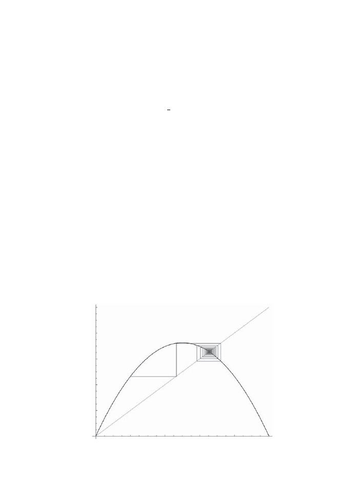
Stability of fixed points
129
Example 16.1: Suppose f(x) = x
2
is a map of the closed interval [0, 1]. Then 0
is a fixed point. It is stable, as f
(0) = 0. But the fixed point at x = 1 is unstable
as f
(1) = 2 > 1. The orbit of 0.99 is driven to zero:
0.99, 0.9801, 0.960596, 0.922745, 0.851458, 0.72498, 0.525596, 0.276252,
0.076315, 0.00582398, 0.0000339187, 1.15048*10
−9
, 1.3236*10
−18
,
· · ·
Example 16.2: The map f(x) =
1
4
x(1
− x) has a stable fixed point at the
origin. Where is its other fixed point? Is it stable?
Example 16.3: But for the case f(x) = 2x(1 − x) the origin is an unstable
fixed point. It has another fixed point at 0.5 which is stable. If we start near
x = 0 we will be driven away from it towards x = 0.5. For example, the orbit of
x
0
= 10
−6
is
0.00100, 0.001998, 0.00398802, 0.00794422, 0.0157622, 0.0310276, 0.0601297,
0.113028, 0.200506, 0.320606, 0.435636, 0.491715, 0.499863, 0.5, 0.5, 0.5, 0.5,
0.5, 0.5, 0.5, 0.5, 0.5, 0.5, 0.5, 0.5, 0.5, 0.5, 0.5, 0.5,
· · ·
A convenient way of displaying the orbit is a cobweb diagram (e.g., Fig. 16.1). Draw
a graph of the function f (x) as well as the identity function, which is the diagonal line
y = x. Start at the point (x
0
, x
1
) on the graph of the function, where x
1
= f (x
0
). Draw a
horizontal line to the point on the diagonal (x
1
, x
1
). Draw a vertical line to the next point
on the graph of the function (x
1
, x
2
), where x
2
= f (x
1
). Repeat by drawing the horizontal
line to (x
2
, x
2
) on the diagonal, a vertical line to (x
2
, x
3
) and so on.
0.2
0.2
0.4
0.6
0.8
1
0.4
0.6
0.8
1
Fig. 16.1
The cobweb diagram of
f(x) = 2.9x(1 − x) with initial point x
0
= 0
.2.

130
Dynamics in one real variable
Differentiable maps of the unit interval f : [0, 1]
→ [0, 1] that satisfy the boundary condi-
tions f (0) = f (1) = 0 must have a maximum between 0 and 1. If there is exactly one such
maximum they are said to be unimodal. Examples are
f (x) = 3x(1
− x), b sin πx, for b < 1
etc. They have an interesting dynamics. It turns out that the special case
f (x) = μx(1
− x)
for various values of the parameter μ represents this class of maps very well. Many of the
properties are universal : independent of the particular unimodal map chosen. So a simple
example will suffice.
An interpretation of this system is that this map represents the time evolution of the
population of some family of rabbits. Let x be the number of rabbits as a fraction of
the maximum number that can be supported by its carrot patch. If x is too close to the
maximum value, the number of rabbits in the next generation will be small: many will die of
starvation. But if x is small, the next generation will have a number proportional to x, the
proportionality constant μ being a measure of the fertility of rabbits.
1
More seriously, it is
possible to construct a non-linear electrical circuit (an analog simulator) which implements
this dynamics.
We will choose 0 < μ < 4 so that the maximum value remains less than one: otherwise
the value f (x) might be outside the interval.
A stable fixed point would represent a self-sustaining population. There are at most two
fixed points:
f (x) = x =
⇒ x = 0, 1 −
1
μ
Note that
f
(0) = μ,
f
1
−
1
μ
= 2
− μ
16.4.1
One stable fixed point:
1 > μ > 0
When μ < 1, the second fixed point is outside the interval, so it would not be allowed. In
this case, the fixed point at the origin is stable:
f
(0) = μ < 1
Every point on the interval is attracted to the origin. The fertility of our rabbits is not
high enough to sustain a stable population.
1
This is crude. But then, it is only an attempt at quantitative biology and not physics.
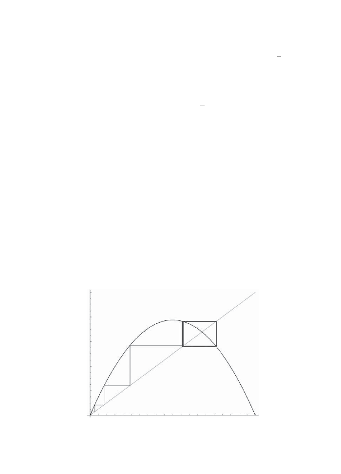
Unimodal maps
131
16.4.2
One stable and one unstable fixed point:
1 < μ < 3
When 1 < μ < 3, the fixed point at the origin is unstable while that at 1
−
1
μ
is stable.
A small starting population will grow and reach this stable value after some oscillations.
For example, when μ = 2.9 this stable value is 0.655172. A population that is close to 1
will get mapped to a small value at the next generation and will end up at this fixed point
again.
16.4.3
Stable orbit of period two :
3 < μ < 1 +
√
6
Interesting things start to happen as we increase μ beyond 3. Both fixed points are now
unstable, so it is not possible for the orbits to end in a steady state near them. A periodic
orbit of period two occurs when μ is slightly larger than 3 (see Fig. 16.2). That is, there is
a solution to
f (f (x)) = x
within the interval. For example, when μ = 3.1 the solutions are
0, 0.558014, 0.677419, 0.764567
The first and the third are the unstable fixed points of f that we found earlier. The
other two values mapped into each other by f and formed a periodic orbit of period two.
f (x
1
) = x
2
,
f (x
2
) = x
1
x
1
≈ 0.558014, x
2
= 0.764567
0.2
0.2
0.4
0.6
0.8
1
0.4
0.6
0.8
1
Fig. 16.2
The cobweb diagram of
f(x) = 3.1x(1 − x) showing a cycle of period 2.

132
Dynamics in one real variable
Is this stable? That amounts to asking whether
|f
2
| < 1 at these points. If f(x
1
) = x
2
,
f (x
2
) = x
1
f
2
(x
1
) = f
(f (x
1
))f
(x
1
) = f
(x
2
)f
(x
1
)
Clearly f
2
(x
2
) is equal to the same thing. So we are asking of the product of the deriva-
tives of f along the points on one period is less than one. Numerically, for μ = 3.1 we get
f
2
(x
1
) = 0.59. This means that the orbit of period two is stable. The population of rabbits
ends up alternating between these values forever, for most starting values.
We can understand this analytically. To find the fixed points of f
2
we must solve the
quartic equation f
2
(x) = x. We already know two roots of this equation (since 0, 1
−
1
μ
are
fixed points of f hence of f
2
). So we can divide by these (that is, simplify
f
2
(x)−x
x
(
x
−1+
1
μ
)
) and
reduce the quartic to a quadratic:
1 + μ
− xμ − xμ
2
+ x
2
μ
2
= 0
The roots are at
x
1,2
=
1 + μ
±
−3 − 2μ + μ
2
2μ
As long as μ > 3 these roots are real: we get a periodic orbit of period two. We can calculate
the derivative at this fixed point as above:
f
2
(x
1
) = 4 + 2μ
− μ
2
For the period two orbit to be stable we get the condition (put f
2
(x
1
) =
−1 to get the
maximum value for stability)
μ < 1 +
√
6
≈ 3.44949
16.4.4
Stable orbit of period four :
3.44949 . . . < μ < 3.54409 . . .
Thus, as μ increases further this orbit will become unstable as well: a period four orbit
develops (see Fig. 16.3). Numerically, we can show that it is stable till μ
≈ 3.54409 . . .
16.4.5
3.54409 . . . < μ < μ
∞
After that, there is a stable period eight orbit until μ
≈ 3.5644 . . . and so on. Let μ
n
be the
value at which a period 2
n
orbit first appears. They form a convergent sequence:
3, 3.44949, 3.54409, 3.5644, 3.568759,
→ μ
∞
≈ 3.568856
The rate of convergence is geometric. Using much more sophisticated methods,
Feigenbaum (1978) obtained
lim
n
→∞
μ
n
− μ
n
−1
μ
n
+1
− μ
n
≡ δ = 4.669 . . .
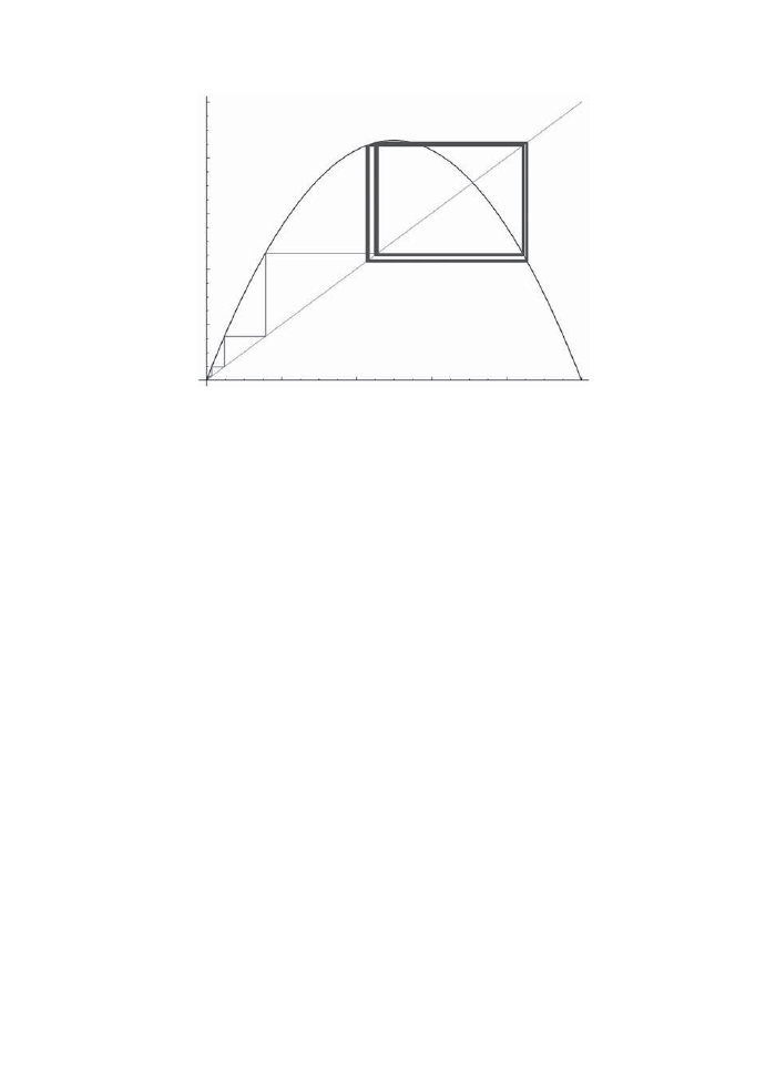
Invariant measures
133
0.2
0.2
0.4
0.6
0.8
1
0.4
0.6
0.8
1
Fig. 16.3
The cobweb diagram of
f(x) = 3.4495x(1 − x) showing a cycle of period 4.
A study of another unimodal map such as f (x) = μ sin πx (restricted to the unit interval)
will lead to a similar, but numerically different, sequence. While studying this, Feigenbaum
made a surprising discovery: although the values at which the period doubles depend on
the choice of f , the rate of convergence is universal : it is always the same mysterious
number 4.669... This reminded him of similar universality in the theory of critical phenom-
ena (such as when a gas turns into a liquid) which had been explained by Wilson using
an esoteric theoretical tool called renormalization. He then developed a version of renor-
malization to explain this universality in chaos, leading to the first quantitative theory of
chaos. In particular, the universal ratio above turns out to be the eigenvalue of a linear
operator.
An important question raised by Boltzmann in the nineteenth century is whether
Hamiltonian systems that are far from being integrable (e.g., the dynamics of a large num-
ber of molecules) are ergodic. Is the fraction of the time that an orbit spends in a domain
of the phase space
2
proportional to its volume? Is this true for almost every orbit? If these
hypotheses hold, we would be able to derive statistical mechanics from Hamiltonian me-
chanics. We are far from a general resolution of these questions. But much progress has been
made in the past century and a half. Many special case have been shown to be ergodic. In
the other direction, the Kolmogorov–Arnold–Moser theorem shows that nearly integrable
systems are not.
2
More precisely, the submanifold of states of a given energy.

134
Dynamics in one real variable
To talk of volumes in phase space, we need a measure of integration that is invariant
under time evolution. We saw that for a Hamiltonian system with a non-degenerate Poisson
bracket, there is an invariant measure (volume) in phase space. In canonical co-ordinates,
this is just
"
i
dp
i
dq
i
. For general dynamical systems, there may not always be such a
measure:
3
the system could be dissipative, so that all orbits concentrate on some small
subset (even a point). But in many cases we can find such an invariant measure.
Example 16.4: For the doubling map f(x) = 2x mod 1, the usual Lebesgue
measure dx on the unit interval is invariant. The reason is that f is a two-to-one
map, with Jacobian 2. Put differently, each interval arises as the image of two
others, each with half the length of the original.
It turns out that the doubling map is indeed ergodic on the unit interval with
respect to this measure. Suppose A is an invariant set of f . That is, if x
∈ A
then f (x)
∈ A as well. An example would be a periodic orbit. This example has
zero measure: A is contained in unions of intervals that can be made as small
as you want. There are also invariant sets of positive measure. For example, the
orbit of an interval [0, ].
A =
∞
.
n
=−∞
f
n
([0, ])
It can be shown that any invariant set of f with positive measure is of full
measure. That is, a set invariant under the dynamics is either of volume zero or
its volume is equal to that of the whole interval. This is a form of ergodicity.
This is just the beginning of a vast area of ergodic theory.
Problem 16.1: Show that for the fully chaotic logistic map f(x) = 4x(1 − x),
the measure
dμ(x) =
dx
π
x(1
− x)
is invariant. (Remember that f is a two-to-one map.)
Problem 16.2: Plot the periodic cycles of the map f(x) = μ sin(πx) letting μ
vary in the range 0 < μ < 1 in small steps (about 10
−2
). For each value of μ,
start with some value of x (e.g., near 0.5) and make a list of a few hundred points
in its orbit, after dropping the first one hundred or so. This should produce a
cycle (see Fig. 16.4). Plot the list of values (μ, x) you get this way.
Problem 16.3: Study the dynamics of the map f(x) = μx(1 − x) for the pa-
rameter range 0 < μ < 4 numerically. Find the first four values of μ at which
the period doubles.
Problem 16.4: Project
∗∗
We can apply the idea of iteration to the space of
unimodal functions itself, by repeating the above construction. The fixed point
3
There may not be an invariant measure that is absolutely continuous w.r.t. the Lebesgue measure.
It might be concentrated at some points, for example.
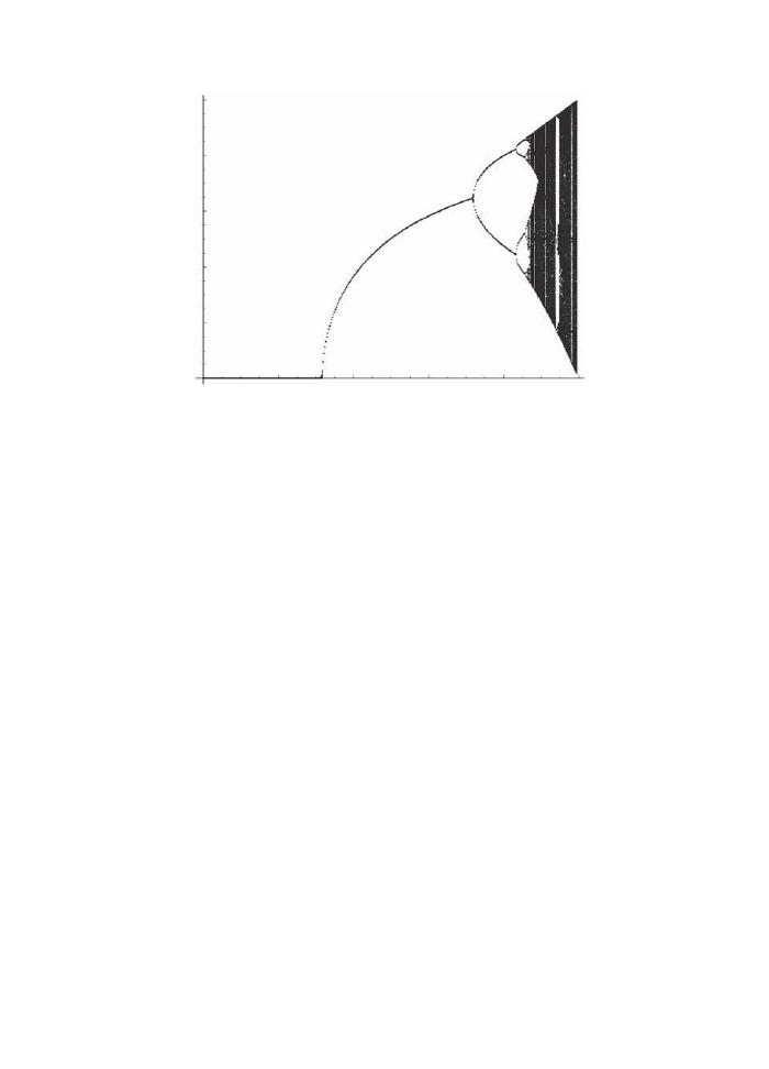
Invariant measures
135
0.2
0.2
0.4
0.6
0.8
1
0.4
0.6
0.8
1
Fig. 16.4
The cycles of the map
f(x) = μ sin(πx) for the range 0 < μ < 1.
will be a universal unimodal function which has an orbit of infinite period. The
constant δ in Section 16.4.5 can be understood as the rate of convergence to
this fixed point. Read Feigenbaum’s article (1978) and verify his results.

This page intentionally left blank

17
Dynamics on the complex plane
There are two natural groups of transformations of the plane. If the areas are preserved we
get canonical (also called symplectic) transformations. If the angles of intersection of any
pair of lines are preserved, we get conformal transformations. These are simply complex
analytic functions. If both areas and angles are preserved, the transformation is an isometry
of the Euclidean metric: a combination of a rotation and a translation. We have already
studied iterations of canonical transformations. In this chapter, we study the iterations of
a complex analytic function of one variable. For a deeper study, see the books by Milnor
(1999), and McMullen (1994).
The simplest analytic functions are polynomials. They are analytic everywhere on the com-
plex plane. At infinity, a polynomial must have infinite value, except in the trivial case where
it is a constant. It is convenient to extend the complex plane by including the point at in-
finity, ˆ
C = C ∪ {∞}. A rational function is of the form R(z) =
P
(z)
Q
(z)
where P (z) and Q(z)
are polynomials (without common factors, because they could be cancelled out). Rational
functions can be thought of as analytic functions mapping ˆ
C to itself: whenever the denom-
inator vanishes, its value is the new point at infinity we added. For example, the function
1
z
−1
can now be thought of as an analytic function that maps
∞ to zero and 1 to ∞.
An important geometric idea is that ˆ
C can be identified with a sphere. More precisely,
there is a coordinate system (the stereographic system) on
S
2
that associates to every point
p on it a complex number; place the sphere on the plane so that its south pole touches the
origin. Draw a straight line from the north pole to p
∈ S
2
; continue it until it reaches the
plane at some point z(p). This is the co-ordinate of p. Clearly the co-ordinate of the south
pole is zero. The equator is mapped to the unit circle. As we get close to the north pole,
the co-ordinate gets larger: the north pole itself is mapped to the point at infinity.
A moment’s thought will show that this map is invertible: to every point on ˆ
C there
is exactly one point on
S
2
. So the sphere is nothing but the complex plane with the point
at infinity added. This point of view on the sphere is named for Riemann, the founder of
complex geometry as well as Riemannian geometry.
Thus, rational functions are complex analytic maps of the sphere to itself. The study
of the dynamics of such maps is an interesting subject. Even simple functions such as
f (z) = z
2
+ c (for constant c) lead to chaotic behavior. But we begin with a simpler case
that is not chaotic.

138
Dynamics on the complex plane
A rotation takes the sphere to itself in an invertible way: each point has a unique inverse
image. It preserves the distances between points. In complex geometry, there is a larger
class of analytic maps that take the sphere to itself invertibly. The rotations are a subset
of these. To determine these we ask for the set of rational functions for which the equation
R(z) = w
has exactly one solution z for each w. This is the same as solving the equation
P (z)
− wQ(z) = 0, R(z) =
P (z)
Q(z)
The number of solutions is the degree of the polynomial P (z)
− wQ(z) in the variable z.
This is the larger of the degrees of P (z) or Q(z): which is called the degree of the rational
function R(z). Thus, for example,
1
z
2
+3
has degree two. So we see that invertible maps
of the sphere correspond to rational functions of degree one; i.e., P (z) and Q(z) are both
linear functions
M (z) =
az + b
cz + d
But, the numerator and denominator should not be just multiples of each other: then M (z)
is a constant. To avoid this, we impose
ad
− bc = 0
Exercise 17.1: Check that ad − bc = 0, if and only if R(z) is a constant.
In fact, by dividing though by a constant, we can even choose
ad
− bc = 1
We are interested in iterating maps, so let us ask for the composition of two
such maps M
3
(z) = M
1
(M
2
(z)). We will often denote this composition of maps
by
◦:
M
3
= M
2
◦ M
1
It must also be a ratio of linear functions: invertible functions compose to
give invertible functions. Calculate away to check that
M
i
(z) =
a
i
z + b
i
c
i
z + d
i
,
i = 1, 2, 3
have coefficients related by matrix multiplication:
a
3
b
3
c
3
d
3
=
a
1
b
1
c
1
d
1
a
2
b
2
c
2
d
2
Dynamics of a Mobius transformation
139
Thus Mobius transformations correspond
1
to the group of 2
× 2 matrices of
determinant one, also called SL(2, C). Rotations correspond to the subgroup of
unitary matrices.
It turns out that the general Mobius transformation is closely related to a
Lorentz transformation in space-time. The set of light rays (null vectors) passing
through the origin in Minkowski space is a sphere. A Lorentz transformation
will map one light ray to another: this is just a Mobius transformation of the
sphere.
If we ask how the ratio of two components of a vector transforms under a
linear transformation, we get a Mobius transformation
ψ
1
ψ
2
→
a b
c d
ψ
1
ψ
2
ψ
1
ψ
2
≡ z →
az + b
cz + d
.
This gives another, algebraic interpretation.
Dynamics of a Mobius transformation
We can now ask for the effect of iterating a Mobius transformation M (z) =
az
+b
cz
+d
. Given an
initial point z
0
, we get an infinite sequence
z
n
= M (z
n
−1
),
n = 0, 1, 2,
· · ·
Because M is invertible, we can also go backwards: define z
−1
as the solution of the equation
M (z
−1
) = z
0
, and similarly z
−2
= M
−1
(z
−1
) and so on. Thus the orbit of a point is a
sequence
z
n
= M (z
n
−1
),
n =
· · · , −2, −1, 0, 1, 2, · · ·
which is infinite in both directions.
Let us find fixed points of M (z):
M (z) = z =
⇒ az + b = z(cz + d)
There are two possible roots for this quadratic equation
z
±
=
a
− d ±
(a
− d)
2
+ 4bc
2c
1
The alert reader will notice that this is a pretty little lie. Mobius transformations actually correspond
to P SL(2, C) = SL(2.C)/
{1, −1}, as reversing the signs of all the components of the matrix does not affect
M (z). What is the subgroup of rotations?

140
Dynamics on the complex plane
The quantity Δ = (a
− d)
2
+ 4bc is called the discriminant. If Δ
= 0, the Mobius
transformation M (z) has two distinct fixed points. Since ad
− bc = 1, we also have
Δ = (a + d)
2
− 4.
Next, we ask if each fixed point is stable. That is, whether
|f
(z
±
)
| < 1. Using again the
fact that ad
− bc = 1 we find that f
(z) =
1
(cz+d)
2
. The solution above gives
f
(z
±
) =
a + d
∓
√
Δ
2
The derivatives are reciprocals of each other:
f
(z
+
)f
(z
−
) = 1
So, if one fixed point is stable, the other unstable. It is also possible for f
to be reciprocal
numbers of magnitude one at the fixed points. Then the fixed points are neutrally stable.
Finally, if the fixed points coincide, f
must be 1.
Collecting the above facts, we see that there are three classes of Mobius transformations:
1. Hyperbolic (also called loxodromic) Two distinct fixed points, where one is stable and
the other unstable. This is the generic case. That is, six independent real numbers are
needed to determine a hyperbolic element: the three complex numbers determining the
positions of the fixed points and the derivative at one of them.
2. Elliptic Two distinct fixed points again, and each is marginally stable. Since the
magnitude of the fixed point must be one, there is a five-real-parameter family
of them.
3. Parabolic There is only one fixed point, at which the derivative is one. There is a four-
parameter family of them: the co-ordinates of the fixed point and the value of the complex
number μ which determines the behavior at a fixed point (see below).
Example 17.1: Here are some examples:
• Hyperbolic
&
2 0
0
1
2
'
,
&
2
e
iθ
e
−iθ
1
'
,
0 < θ < 2π
• Elliptic
&
e
iθ
b
0
e
−iθ
'
,
0 < θ < 2π
• Parabolic
&
1 0
4 1
'

The map z
→ z
2
141
17.3.1
The standard form of a Mobius transformation
We say that two Mobius transformations M
1
, M
2
are equivalent if there is another Mobius
transformation S such that
M
2
= S
◦ M
1
◦ S
−1
S will map the fixed points of M
1
to those of M
2
. If M is not parabolic, we can find an
S that moves one of the fixed points to the origin and the other to infinity; just choose
S =
1
√
z
−
−z
+
z
−
z
+
1
1
. If M
1
is parabolic, we can choose S so that the fixed point of M
2
is at infinity. This way we can bring a Mobius transformation M to a standard form in
each case:
1. Hyperbolic S
◦ M ◦ S
−1
=
λ 0
0 λ
−1
,
|λ| < 1,
z
→ λ
2
z
2. Elliptic S
◦ M ◦ S
−1
=
&
e
i
θ
2
0
0 e
−i
θ
2
,
'
,
0 < θ < 2π.
z
→ e
iθ
z
3. Parabolic S
◦ M ◦ S
−1
=
1 0
μ 1
,
z
→
z
μz
+1
This is useful because it is easy to determine the orbits of these standard forms. We can
then transform back to determine the orbits of the original M .
The orbits of z
→ λ
2
z are spirals converging to the origin. When λ < 1, the origin is
stable and infinity is unstable. The transformation z
→ e
iθ
z is a rotation around the origin.
The orbits lie along a circle. The parabolic transformation z
→
z
μz
+1
has orbits converging
to the origin.
Once we know the orbits of the standard form, we can determine those of the general
case by applying S. Or we can simply plot some examples numerically.
Let us look at the simplest map of degree 2
z
→ z
2
Clearly, any point in the interior of the unit circle will get mapped to the origin after
many iterations. Any point outside the unit circle will go off to infinity. On the unit circle
itself, we get the doubling map we studied in the last chapter:
z = e
2πix
,
x
→ 2x mod 1
We saw that the latter is chaotic: an irrational value of x has a completely unpredictable
orbit. But these are most of the points on the unit circle. Even the periodic orbits (rational

142
Dynamics on the complex plane
numbers with a denominator that is a power of two) have something wild about them: they
are all unstable. The unit circle is the union of such unstable periodic points. This is a
signature of chaotic behavior.
Thus the complex plane can be divided into two types of points:. Those not on the unit
circle, which get mapped predictably, and those on the unit circle whose dynamics is chaotic.
We will see that points on the plane can always be classified into two such complementary
subsets. The chaotic points belong to the Julia set and the rest belong to the Fatou set.
But, in general, the Julia set is not necessarily something simple like the unit circle. Often,
it is a quite intricate fractal.
For example, the Julia set of the map z
→ z
2
+ i is a “dendrite”: a set with many
branches each of which are branched again. Why does this happen? The key is that at its
fixed point (which is unstable), the derivative is not a real number. That is, near the fixed
point, the map is both a scaling (stretching) and a rotation. The orbits are spirals. Such a
set cannot lie in a smooth submanifold of the plane (unless it consists of the whole plane).
So, whenever we have an unstable fixed point with a derivative that is not real (and we
know that the domain of repulsion is not the whole plane) the Julia set will be some kind
of fractal. This is very common.
How do we come up with a definition of when an orbit is chaotic and when it is not?
That is, which points belong to the Julia set and which to the Fatou set? A more precise
definition is needed to make further progress.
We will need a notion of convergence of maps to make sense of this idea; and also a
notion of distance on the Riemann sphere that is invariant under rotations.
In spherical polar co-ordinates, the distance between neighboring points on the sphere is
ds
2
= dθ
2
+ sin
2
θdφ
2
The stereographic co-ordinates are related to this by
z = cot
θ
2
e
iφ
Rewritten in these co-ordinates the metric is
ds
2
=
4
|dz|
2
(1 + z ¯
z)
2
The distance s between two points z
1
, z
2
can be calculated from this by integration
along a great circle. For our purposes, an equally good notion of distance in the length d of
the chord that connects the two points. Some geometry will give you the relation between
the two notions:

Metric spaces
143
d = 2 sin
s
2
d(z
1
, z
2
) =
2
|z
1
− z
2
|
(1 +
|z
1
|
2
)(1 +
|z
2
|
2
)
The advantage of these notions of distance over the more familiar
|z
1
− z
2
| is that they
are invariant under rotations. For example, the point at infinity is at a finite distance:
d(z,
∞) =
2
(1 +
|z|
2
)
We only care about the topology defined by the distance, which is the same for d and s:
that is, when one is small the other is also. So any sequence that converges in one will
converge in the other. It is a matter of convenience which one we use in a computation.
Metric is another word for distance. A metric d on a set X is a function d : X
× X → R
such that
1. d(x, x) = 0
2. d(x, x
) > 0 if x
= x
Positive
3. d(x, x
) = d(x
, x) Symmetry
4. d(x, x
)
≤ d(x, x
) + d(x
, x
) The triangle inequality
The most obvious example is the case of Euclidean space X =
R
n
and
d(x, x
) =
|x − y| =
/
0
0
1
n
i
=1
(x
i
− x
i
)
2
The chordal distance (the length of the chord connecting two points) on the sphere is
another example of a metric.
Exercise 17.2: Prove the triangle inequality for the chordal distance.
The metric is a useful concept because it allows us to speak of convergence.
We say that x
n
∈ X converges to x if for every there is an N such that
d(x
n
, x) < for n
≥ N. It also allows us to speak of a continuous function.
A function f : X
→ Y from one metric space to another is continuous if for
every > 0 there is a δ such that
d
Y
(f (x), f (x
)) < δ, for d
X
(x, x
) <
That is, we can make the values of a function at two points as small as we
want by bring the points close enough.

144
Dynamics on the complex plane
17.6.1
Compactness
Not every sequence converges. The points might move farther and farther away from the
initial one as n grows. Or they might wander, approaching one point then another and
back to the first and so on. In the latter case, there would be a subsequence with a limit.
A compact set is one in which every sequence has a convergent subsequence.
Continuous functions on compact sets have many of the properties that a function on
a finite set would have. For example, a real-valued function on a compact set is bounded.
This is why it is so important: compactness allows us to treat some very large, infinite,
sets as if they are finite. It makes sense to speak of the supremum (roughly speaking the
maximum value; more precisely the least upper bound) or the infimum (least greatest lower
bound) of a function on a compact set. These notions do not make sense if the domain is
non-compact.
Example 17.2: The reciprocal is a continuous function on the open interval
(0, 1). It does not have a supremum: it grows without bound near 0. Thus,
the open interval is not compact. On the other hand, the closed interval
[0, 1] =
{x|0 ≤ x ≤ 1} is compact. Any continuous function on it is bounded.
The reciprocal is not a continuous function on the closed interval.
17.6.2
Distance between functions
Often we will need to ask whether a sequence of functions has a limit. (For example, does a
power series converge in some domain? This is the same as asking if the sequence of partial
sums converge to some function.) It is useful in this case to have a notion of distance
between functions. If the domain K is compact, we can take the largest distance between
the values of the functions and declare that to be the distance between functions themselves
d(f, g) = sup
x
∈K
d(f (x), g(x))
This turns the set of functions into a metric space as well, allowing us to speak of convergence
of a sequence of functions. A normal family is a set of functions such that every infinite
sequence in it has a convergent subsequence. In other words, it is a compact subset of the
metric space of functions.
When do the iterates f, f
2
, f
3
,
· · · of an analytic function f tend to a limit φ that is also
an analytic function? This question is important because if such a limiting function exists,
the dynamics would be easy to understand: it would not be chaotic.
This is where we will use the idea of convergence of sequences of functions from the
previous section. So we define the Fatou set of f to be the largest domain on which the
iterates f
n
have a subsequence that converges to an analytic function φ. That is the largest
domain on which the iterates form a normal family. The complement of the Fatou set is
the Julia set. On it, the dynamics are chaotic. Here are some theorems about the Julia set
that help to explain what it is. Look at the books by Milnor (1999) and McMullen (1994)
for proofs and a deeper study.

Julia and Fatou sets
145
Theorem 17.1: Let J be the Julia set of some analytic function f : S
2
→ S
2
.
Then, z
∈ J, if and only if its image f(z) ∈ J as well.
Thus, the Julia set is invariant under the dynamics; the Julia set of f and
those of its iterates f
n
are the same.
Theorem 17.2: Every stable periodic orbit is in the Fatou set. However, every
unstable periodic orbit is in the Julia set.
Recall that if z is in a periodic orbit of period k, we have f
k
(z) = z. It is
stable if
|f
k
(z)
| < 1 and unstable if |f
k
(z)
| > 1. There is a neighborhood of
every periodic orbit in which all points will get closer and closer to the periodic
orbit as we iterate f . This is called the basin of attraction of the orbit.
Theorem 17.3: The basin of attraction of every stable periodic point is in the
Fatou set. Roughly speaking, the Fatou set consists of all the stable periodic
orbits and their basins of attraction. On the other hand . . .
Theorem 17.4: The Julia set is the closure of the set of unstable periodic orbits.
This means that every point in the Julia set can be approximated as close as we
want by some unstable periodic point.
It is useful to have a characterization of the Julia set that allows us to
compute it.
Theorem 17.5: If z
0
is in the Julia set J of some analytic function f , then
the set of pre-images of z
0
is everywhere dense in J .
That is, the Julia set is well-approximated by the set
z
∈ S
2
: f
n
(z) = z
0
, n
≥ 1
where f
n
is the nth iterate of f . So to compute a Julia set, we must first find one point
z
0
on it. (For example, pick an unstable fixed point). Then we solve the equation f (z) = z
0
to find the first set of pre-images. If f (z) is a rational function, this amounts to solving
some polynomial equation, which has some finite number of solutions. Then we find all
the pre-images of these points and so on. The number of points grows exponentially. If we
plot them, we get an increasingly accurate picture of the Julia set. The point in doing this
“backwards evolution” is that it is stable. Precisely because f is unstable near z
0
, its inverse
is stable: we can reliably calculate the solutions to f (z) = z
0
since the errors in z
0
will be
damped out in the solutions.
In practice, it might make sense to pick just one pre-image at random at each step.
This way, we can search in depth and not be overwhelmed by the exponential growth of
pre-images. Although the picture of the Julia set you get this way is not as pretty as some
others you will see, it is more representative of the dynamics. Areas that are visited often
will be darker (see Fig. 17.2). For more on these matters see Milnor (1999).
Problem 17.3: What is the relation between the fixed points of a Mobius
transformation and the eigenvectors of the corresponding matrix? Same for the
eigenvalues and the derivatives of the Mobius transformation at a fixed point.
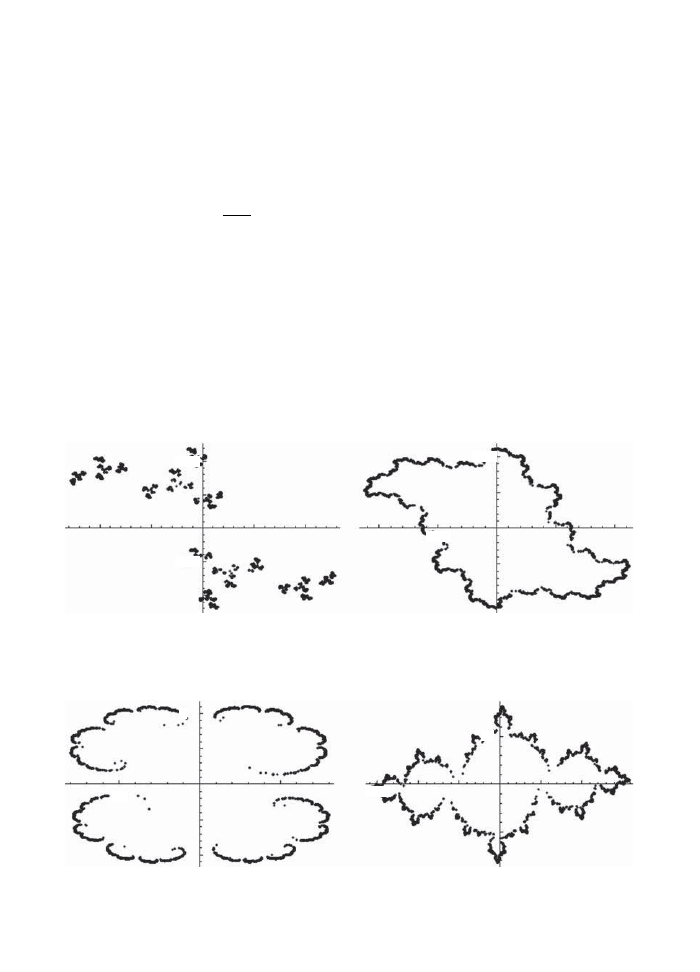
146
Dynamics on the complex plane
Compare the classification of Mobius transformations to Jordan canonical forms
of matrices. When can a matrix not be diagonalized?
Problem 17.4: Find a Mobius transformation that has fixed points at given
points z
u
, z
s
and has derivative at z
s
equal to λ. Plot some orbits of
the hyperbolic Mobius transformation with z
u
= 2.0 + 2.1i, z
s
=
−8 − 10.1 i,
λ = 0.9896
− 0.0310997 ∗ i. Plot orbits of the parabolic Mobius transformation
(see Fig. 17.3) z
→
z
μz
+1
for some values of μ.
Problem 17.5: Write a program that will plot the Julia set of the map
P (z) = z
2
+ c for different choices of c, such as those plotted in Figure 17.1.
Problem 17.6: The Mandelblot The Mandelbrot set is the set of all values of
the parameter c for which the orbit of 0 under the above map remains bounded
z
n
(c) = z
2
n
−1
(c) + c,
z
0
(c) = 0
M =
{c|∃s > 0, ∀n, |z
n
(c)
| < s}
–0.5
–1.0
–1.0
0.5
1.0
–1.0
–0.5
0.5
1.0
0.115603 + i
0.115603 + 0.51942i
–0.5
0.5
1.0
–1.0
–0.5
0.5
1.0
Fig. 17.1
Julia sets for
z
2
+
c for various values of c.
–1.0
–0.5
0.5
1.0
–0.5
0.5
0.335121 + 0.0149522i
–0.913785 – 0.0923379i
–0.5
0.5
–1.0
–1.5
–0.5
0.5
1.0
1.5
Fig. 17.2
More Julia sets.
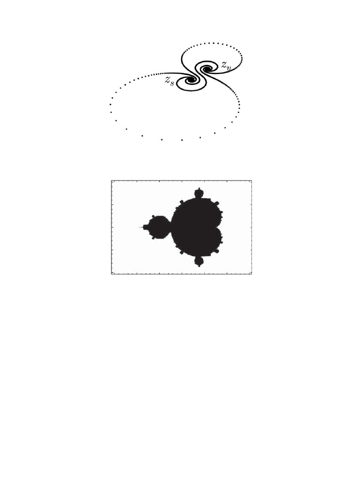
Julia and Fatou sets
147
Fig. 17.3
Orbits of a hyperbolic Mobius transformation.
–2.0
–1.0
–0.5
0.0
0.5
1.0
–1.5
–1.0
–0.5
0.0
0.5
1.0
Fig. 17.4
The Mandelbrot set.
This set has a visually amazing fractal structure. Write a program that plots
the Mandelbrot set (Fig. 17.4). You can also color code it by the number of
iterations it takes for the orbit to leave the range of the plot.

This page intentionally left blank

The Kolmogorov–Arnold–Moser (KAM) theorem of mechanics places limits on when chaos
can set in. It gives conditions under which an integrable system can be perturbed and re-
main predictable. This is a deep theory with many mathematical difficulties. So we will work
up to it by solving a couple of much easier problems in this chapter. We will use Newton’s
ancient iteration method to solve the problem of diagonalizing matrices, and to bring dif-
feomorphisms of the circle to normal form. The first doesn’t really have much to do with
chaos; it is only included as a warm-up exercise. The second is a toy model for mechanics.
More detailed exposition can be found in Wayne (2008), Celletti and Chierchia (2007) and
Arnold (1961 and 1989).
The essential difficulty to overcome is that of small denominators in perturbation the-
ory. If you are close to a resonance, a small perturbation can have a large effect, in the
linear approximation. More precisely, the measure of the size of a perturbation must take
into account the effect of possible resonances. Once the correct measure of the size of a
perturbation is found, a Newton’s iteration solves the problem.
One of the earliest uses of iterations is to solve non-linear equations. Suppose we want to
solve an equation f (α) = 0 in one variable (real or complex). Given a guess x for the root,
Newton’s method is to solve the first order approximation
0 = f (α)
≈ f(x) + f
(x)(α
− x)
to get an improved guess:
α
≈ x − [f
(x)]
−1
f (x)
We then repeat the whole process. In other words, we iterate the function
R(x) = x
− [f
(x)]
−1
f (x)
The sequence x
k
+1
= R(x
k
) converges if the initial guess x
0
is close enough to a root and
f
(x
k
) does not ever become small.
The method even applies to the case of several variables, except that x
k
are now vectors
and f
(x) is a matrix. Again, there are problems if the matrix has small eigenvalues; that

150
KAM theory
is, if its inverse becomes large. (The problem of small denominators.) Indeed, this method
even generalizes to infinite-dimensional spaces, provided we have a way of measuring the
length of a vector and hence a norm for operators; for example, to Hilbert or Banach spaces.
18.1.1
Proof of convergence
We will show that as long as
f
(x)
= 0
(18.1)
along the orbit, the Newton iteration will converge.
A measure of how far away we are from a root is given by
δ(x) =
|R(x) − x|
where
R(x) = x
− r(x), r(x) =
f (x)
f
(x)
Under an iteration, it changes to
δ(R(R(x))
− R(x)) = |r(R(x))| = |r(x − r(x))| ≈ |r(x)[1 − r
(x)]
| = δ(x)|1 − r
(x)
|
But
1
− r
(x) =
f (x)f
(x)
f
2
(x)
=
f
(x)
f
(x)
r(x)
Thus we have
δ(x
k
+1
)
≈
22
22
f
(x
k
)
f
(x
k
)
22
22 δ
2
(x
k
)
so that the error decreases quadratically as long as the criterion 18.1 is satisfied. That is,
at each step, the error is roughly the square of the error in the previous step.
Suppose we are given a matrix L. When is there an invertible linear transformation
(similarity transformation) S that will bring L to diagonal form?
S
−1
LS = Λ,
Λ =
⎛
⎝
λ
1
0
· · ·
0
λ
2
· · ·
·
· · · ·
⎞
⎠
(18.2)
Not every matrix can be diagonalized. It is not even true that small perturbations of
diagonal matrices can always be diagonalized.

Diagonalization of matrices
151
Example 18.1:
L =
1
0
1
cannot be diagonalized for
= 0, no matter how small is.
Small perturbations of diagonal matrices with unequal diagonal entries (non-
degenerate eigenvalues) can be diagonalized. One approach to this is to use
Newton’s iteration.
Define a quantity that measures the size of the off-diagonal part
δ(L) =
i
=j
|L
ij
|
|L
ii
− L
jj
|
Notice that each off-diagonal element is compared to the difference of the cor-
responding diagonal entries. Thus, a matrix like that in the above example will
never have small δ(L): we would need the diagonal entries to be unequal for
that.
We will now construct a similarity transformation that makes δ(L) smaller,
assuming it started off small. As in Newton’s method, this is found by solving
the linear approximation to the equation 18.2.
Let
S = 1 + s,
s
ij
= 0 for i = j
To first order in s, S
−1
≈ 1 − s. Treating the off-diagonal entries of L as small
as well, 18.2 gives
L
ij
≈ (L
jj
− L
ii
)s
ij
, for i
= j
When δ(L) is small, L
ii
= L
jj
and the solution
s
ij
≈
L
ij
L
jj
− L
ii
;
i
= j, s
ii
= 0
(18.3)
can be found. Moreover, the size of s is small:
|s| ≡
i
=j
|s
ij
| = δ(L)
Thus, we define
[S(L)]
ii
= 1,
[S(L)]
ij
=
L
ij
L
jj
− L
ii
, for i
= j
Now we define an iteration as in Newton’s method
R(L) = S(L)
−1
LS(L)

152
KAM theory
If δ(L) is small enough, at each step it will become even smaller. Eventually we will get a
diagonal matrix to high precision. We skip a proof and instead ask the reader to work out
a few examples.
Example 18.2: Even for a matrix with fairly close diagonal entries and not
small of-diagonal entries,
L =
&
1.
1.63051
4.75517
1.01
'
,
δ(L) = 212.855
we get a sequence of L’s
&
0.960004 1.6303
4.75455
1.05
'
,
&
0.870106
−1.6286
−4.74959 1.13989
'
,
&
0.602832 1.61341
4.70531 1.40717
'
,
&
−0.138342 −1.48672
−4.33582 2.14834
'
,
&
−1.40089 0.820858
2.39393
3.41089
'
,
&
−1.77733 −0.0642183
−0.187284
3.78733
'
,
converging to
&
−1.77949
0.0000249329
0.0000727137
3.78949
'
,
δ(L) = 0.0000175341.
in just seven iterations.
The point is not that this is a numerically efficient way of diagonalizing a
matrix; it may not be. It is a toy model for the much harder problem of bringing
non-linear maps to a standard (also called normal) form.
Remark 18.1: A small modification of the above procedure will ensure that
the transformation S(L) is unitary when L is hermitian. We choose s as before
(18.3) but put
S =
1 +
1
2
s
1
−
1
2
s
−1
Consider a map of the circle to itself with w
> 0 and
w(θ + 2π) = θ + 2π
Such a map is called a diffeomorphism: a smooth invertible map of the circle. The simplest
example is a rotation
w(θ) = θ + ρ
some constant ρ.

Normal form of circle maps
153
Example 18.3: If
ρ
2π
=
m
n
for a pair of co-prime integers, the orbit of the
rotation θ
→ θ + ρ is periodic with period n. If
ρ
2π
is irrational, the orbit is
dense. That is, every orbit will come as close to a given point as you want.
∀ θ, θ
0
and > 0,
∃n such that |θ
0
+ nρ
− θ| <
Is there a change of co-ordinate θ
→ S(θ) that reduces a generic diffeomor-
phism to a rotation?
S
−1
◦ w ◦ S(θ) = θ + λ
(18.4)
This is also called the normal form of the diffeomorphism. This is analogous to
asking if a matrix can be brought to diagonal form by a change of basis. The
number λ is analogous to the spectrum of the matrix.
Example 18.4: The doubling map θ → 2θ mod 2π cannot be brought to normal
form.
This question is important because such a normalizable diffeomorphism can-
not be chaotic: up to a change of variables, it is just a rotation. The orbit can
be dense, but it will be as predictable as any rotation. Thus, a theorem that
characterizes normalizable maps puts limits on chaos. The surprise is that rota-
tions with rational
ρ
2π
are unstable: there are perturbations of arbitrarily small
size which are chaotic. If the rotation is “irrational enough”, it has a neighbor-
hood in which all the maps are normalizable and hence non-chaotic. The more
irrational the rotation is, the larger this neighborhood. We will soon see how to
measure the irrationality of a rotation.
Again, we can gain some insight by studying the linear approximation to the
problem. We can split w(θ) as a rotation plus a periodic function of zero mean:
w(θ) = θ + ρ + η(θ),
2π
0
η(θ)dθ = 0,
η(θ + 2π) = η(θ)
Clearly,
ρ =
1
2π
2π
0
[w(θ)
− θ]dθ
We can similarly split S to the identity plus a correction
S(θ) = θ + s(θ),
s(θ + 2π) = s(θ)
Treating s and η as small, the first order approximation to 18.4 is
s(θ + ρ)
− s(θ) = η(θ)
(18.5)
To see this, write 18.4 as w(θ + s(θ)) = θ + λ + s(θ + λ). To first order, λ
≈ ρ
and w(θ + s(θ))
≈ θ + ρ + s(θ) + η(θ).
Adding a constant to the solution of 18.5 yields another solution. We can
add such a constant to set s(0) = 0.

154
KAM theory
As they are periodic functions we can expand them in a Fourier series:
η(θ) =
n
=0
η
n
e
inθ
,
s(θ) =
n
s
n
e
inθ
The n = 0 is absent in η because it has zero average.
[e
inρ
− 1]s
n
= η
n
,
n
= 0
(18.6)
We can determine s
0
by the condition that s(0) = 0.
s(θ) =
n
=0
η
n
e
inθ
− 1
e
inρ
− 1
If ρ =
m
n
2π for pair of integers, e
inρ
− 1 would vanish. Thus, to solve equation
18.5,
ρ
2π
should not be a rational number. This is analogous to the condition in
the last section that the diagonal entries of L should be unequal. Now we see
how to define a measure of how far away w is from a rotation
sup
θ
|s(θ)| ≤ δ(ρ, η) ≡
n
=0
2
|η
n
|
|e
inρ
− 1|
Given ρ, η
n
, we thus set
w(θ) = θ + ρ +
n
=0
η
n
e
inθ
,
S(θ) = θ +
n
=0
η
n
e
inθ
− 1
e
inρ
− 1
Then we find ˜
w = S
−1
◦ w ◦ S as the solution of
w(S(θ)) = S( ˜
w(θ))
This allows us to determine the new ˜
ρ, ˜
η
n
as
˜
ρ =
1
2π
2π
0
[ ˜
w(θ)
− θ]dθ, ˜η
n
=
1
2π
2π
0
[ ˜
w(θ)
− θ]e
inθ
dθ,
n
= 0
If δ(ρ, η) is small enough, δ( ˜
ρ, ˜
η) will be of order δ
2
(ρ, η). By iterating this, we
will converge to a pure rotation: the convergence is quadratic as is typical with
Newton’s method.
Example 18.5: The diffeomorphism
w(θ) = θ +
√
2π +
1
3
[cos θ
− sin(2θ)]
has δ
≈ 0.76. It can be reduced to a rotation by λ ≈ 4.45272 (to an accuracy
δ < 10
−10
) in about seven iterations. The resulting rotation number λ is close
to the initial value
√
2π
≈ 4.44288.
So, we see that there is a neighborhood of an irrational rotation that is not
chaotic. How big is this neighborhood for a given irrational number
ρ
2π
? This is
a very interesting problem in number theory.

Diophantine approximation
155
Set ρ = 2πr. For any pair of integers m, n,
e
2πinr
= e
2πi[nr−m]
Thus
22
e
inρ
− 1
22
= 2
| sin π(nr − m)|
So the question is, how small can nr
− m get, for a given r? If r is rational, it can vanish.
For irrational numbers, it can get quite small, when r
≈
m
n
.
An irrational number is said to be of Diophantine exponent a if
22
2r −
m
n
22
2 >
C(r, )
n
a
+
,
∀m, n ∈ Z, > 0
for some C that can depend on r, but not m, n. Note the direction of the inequality. We
are saying that the error in approximating r by rationals should not be too small.
There are some numbers (e.g., e or
#
∞
n
=0
10
−n!
) which do not satisfy this condition
for any a, no matter how big. They are called Liouville numbers. They are not “irrational
enough”: they are too well-approximated by rationals. Such numbers are always either
rational or transcendental (do not satisfy finite order polynomial equations with integer
coefficients), but most transcendental numbers are believed to have a finite Diophantine
exponent.
A theorem of Roth says that irrational algebraic numbers (solutions of polynomial
equations with integer coefficients, like
√
2 or
1+
√
5
2
) are of exponent 2: the errors in ap-
proximating them by rationals only decrease as some power of the denominator. They are
“irrational enough”.
Note that
| sin πx| > |2x| for |x| <
1
2
. Suppose r is type of (C, a). We can pick an m that
makes
|nr − m| small for each n (certainly less than a half) to get
22
e
2πinρ
− 1
22
= 2
|sin[π(nr − m)]| > 4|nr − m| >
4C
n
a
−1
Thus
δ(ρ, η
n
) <
1
4C
n
=0
|η
n
|n
a
−1
In order for δ(w) to be small, the high frequency components of w must fall off fast. The
better the number
ρ
2π
is approximable rationally (a large, C small), the more stringent the
condition on the perturbation η. Thus, the rotations by such angles are more unstable:
smaller corrections can become non-normalizable and hence chaotic.
The conclusion is that even small perturbations to a rotation θ
→ θ + ρ can be chaotic
if
ρ
2π
is rational or is a Liouville number. But if
ρ
2π
is an irrational algebraic number, there
is a neighborhood of perturbations that remains non-chaotic.

156
KAM theory
Recall that an integrable system is one for which there is a canonical transformation
(p
i
(P, Q), q
i
(P, Q)) such that the hamiltonian H(p(P, Q), q(P, Q)) depends only on the mo-
mentum (also called action) variables P
i
. Such a canonical transformation is generated by
S(P, q) which solves the Hamilton–Jacobi equation 10.3. The functions (p
i
(P, Q), q
i
(P, Q))
are found by solving 10.2. The Hamilton’s equations become 10.1. The frequencies ω
i
(P )
will depend on the quantities P . It is only for linear systems (harmonic oscillator) that they
are constants in phase space.
If the orbit is bounded, these variables Q
i
are angles. By convention they are chosen
to have the range [0, 2π]. Thus, for each value of P
i
there is an invariant torus whose co-
ordinates are Q
i
. The nature of the orbit on the invariant torus depends on whether the
frequencies are commensurate. The frequency vector ω
i
(P ) is commensurate if there are
integers such that
i
n
i
ω
i
(P ) = 0
This means that some of the frequencies are in resonance. We will see that this case is
unstable: there are small perturbations to the hamiltonian that can spoil the integrability.
It is important that the frequencies depend on the action variables. So immediately close
to resonant tori there will be others which are not resonant: changing I
i
can lead to some
small shift in frequency that takes us off resonance.
Example 18.6: For a system with just two degrees of freedom
n
1
ω
1
(I) + n
2
ω
2
(I) = 0
has a solution precisely when
ω
2
ω
1
(I) is a rational number. In this case, the orbits
are periodic. If there are no such integers, the orbit is dense: it can come as close
to any point in the torus as you want.
18.5.1
Perturbations of integrable systems
Consider now a system that is close to being integrable. That is, we can find canonical
variables such that the dependence on the angle variables is small. We can expand in a
Fourier series
H(P, Q) = H
0
(P ) +
n
=0
H
n
(P )e
in.Q
≡ H
0
(P ) + h(P, Q)
As in the previous examples, even small perturbations can lead to chaos if there are
resonances. The correct measure of the size of the perturbations turns out to be
δ(H, P ) =
n
=0
|H
n
|
|n · ω(P )|
Note that this quantity depends not just on the hamiltonian H but also on the value of
the nearly conserved quantities P . It is possible for the perturbation to have a small effect
Hamiltonian systems
157
in some regions of the phase and a big (chaotic) effect in other regions. In the regions
where δ(H, P ) is small enough, we will be able to solve the Hamilton–Jacobi equation by
Newton’s iteration. Thus in those regions we would have found a canonical transformation
that brings it to the integrable form and the system is not chaotic. The tricky part is that
the regions where δ(H, P ) is small and those where it is large are not well-separated: they
interlace each other, so that the chaotic boundary is often some fractal.
So we seek a canonical transformation (P.Q)
→ (P
, Q
) generated by some function
S(P
, Q) satisfying the H–J equation.
H
∂S(P
, Q)
∂Q
, Q
= E
We solve this by Newton’s iteration. As always we start with the solution of the linear
approximation. We make the ansatz
S(P
, Q) = P
i
Q
i
+ s(P
, Q)
The first term simply generates the identity map. The second term is the correction.
H
0
P
+
∂s(P
, Q)
∂Q
+ h
P
+
∂s(P
, Q)
∂Q
, φ
= E
The linear approximation is then
ω
i
(P
)
∂s
∂Q
i
+ h(P
, Q) = constant
If we expand in Fourier series
s
n
(P
, Q) =
n
=0
s
n
(P
)e
in.Q
this becomes
in
· ω(P
) s
n
(P
) + h
n
(P
) = 0,
n
= 0
The solution is
s
n
(P
) = i
h
n
(P
)
n
· ω(P
)
Now we see that there will be a divergence due to resonance if the denominator becomes
small. Also the quantity δ(H, P
) that measures the size of the perturbation is simply the
l
1
norm of the sequence s
n
.
n
=0
|s
n
(P
)
| = δ(H, P
)

158
KAM theory
Now we make the change of variables implied by this generated function:
Q
k
= Q
k
+
∂s(P
, Q)
∂P
k
,
P
k
= P
k
+
∂s(P
, Q)
∂Q
k
We solve this equation (without any further approximations) to determine (P, Q) as fun-
ctions of (P
, Q
). substituting into H will give us a new hamiltonian
H
(P
, Q
) = H(P (P
, Q
), Q(P
, Q
))
If δ(H, P ) is small enough, δ(H
, P
) will be even smaller. Typically it will be of order
δ
2
(H, P ). So we can repeat the whole process over again, converging to some integrable
hamiltonian, valid for the region where δ(H, P ) is small.
There have been many refinements to this theory in recent years. It is possible to solve
the problem by a convergent power series rather than an iterative procedure. Chaos can be
shown to be limited in realistic problems in astronomy (Celletti and Chierchia, 2007) such
as the Sun–Jupiter–Asteroid three body problem.
Problem 18.1: Write a program that can find a root of a function of one
variable using Newton’s method. Try out the method for some choices of the
function and the initial value.
f (x) = x
− 1.5 sin(x),
f (x) = (1.166 + 1.574i) + (0.207 + 0.9726i)x + (0.7209 + 0.0099i)x
6
Problem 18.2: Write a numerical program that diagonalizes a matrix with
unequal diagonal entries using the method of this chapter. Test it on the example
given above.
Problem 18.3: Write a symbolic/numerical program that brings a diffeomor-
phism of the circle with small δ to the normal form. (The solution for ˜
w, as
well as the evaluation of integrals, should be done numerically.) Test it on the
example given above.
Problem 18.4: Research project
∗∗∗
Consider the circular restricted three body
problem. Treat the smaller primary as causing the perturbation. Express the
hamiltonian in terms of the action-angle variables of the two body problem
(Delaunay). Implement the KAM iteration in a symbolic/numerical program.
Show that the procedure converges to sufficient accuracy for a realistic problem
(Celletti and Chierchia, 2007) (Sun–Jupiter–Victoria).

Arnold, V.I. (1961). Small denominators: Mappings of the circumference onto itself. AMS Trans-
lations,
46(1965), 213–88.
Arnold, V.I. (1978). Ordinary Differential Equations (1st edn). MIT Press, Cambridge, MA.
Arnold, V.I. (1989). Mathematical Methods of Classical Mechanics (2nd edn). Springer, New York,
NY.
Birkhoff, G.D. (1922). Surface transformations and their dynamical applications. Acta Math.,
43,
1–119.
Celletti, A. and Chierchia, L. (2007). KAM stability and celestial mechanics. Memoirs of the
AMS ,
187(878), 1–134.
Connes, A. (1994). Non-Commutative Geometry (1st edn). Academic Press, San Diego, CA.
Feigenbaum, M. (1978). Quantitative universality for a class of non-linear transformations. J. Stat.
Phys.,
19, 25–52.
Feynman, R.P. (1948). Space-time approach to non-relativistic quantum mechanics. Reviews of
Modern Physics,
20, 367–87.
Landau, L.D. and Lifshitz, E.M. (1977). Mechanics (3rd edn). Pergamon Press, Oxford.
Lefschetz, N. (1977). Differential Equations: Geometric Theory (2nd edn). Dover Press, New York,
NY.
McKean, H. and Moll, V. (1999). Elliptic Curves: Function Theory, Geometry, Arithmetic (1st
edn). Cambridge University Press, Cambridge, UK.
McMullen, C.T. (1994). Complex Dynamics and Renormalization (1st edn). Princeton University
Press, Princeton, NJ.
Milnor, J. (1999). Dynamics in One Complex Variable (1st edn). Vieweg, Wiesbaden.
Montgomery, R. (2005). Hyperbolic pants fit a three-body problem. Ergodic Theory and Dynamical
Systems,
25, 921–47.
Rajeev, S.G. (2008). Exact solution of the Landau–Lifshitz equations for a radiating charged
particle in the Coulomb potential. Ann. Phys.,
323, 2654–2661.
Strogarz, S.H. (2001). Nonlinear Dynamics and Chaos (1st edn). Westview Press, Boulder, CO.
Sudarshan, E.C.G. and Mukunda, N. (1974). Classical Dynamics: A Modern Perspective (1st edn).
John Wiley, New York, USA.
Wayne, C.E. (2008). An Introduction to KAM Theory. Unpublished. Avaliable at http://math.
bu.edu/people/cew/preprints/introkam.pdf.
Yoshida, H. (1990). Construction of higher order symplectic integrators. Phys. Lett.,
A150, 262–8.

This page intentionally left blank

A
Action, 3
Airy, 87
Arithmetic-Geometric Mean, 18
Arnold, 87, 123, 149
Aryabhatiya, 58
Associative, 46
Asteroid, 158
Asymptotic Freedom, 40
Attactor
strange, 41
Axioms, 113
B
Baker–Campbell–Hausdorff, 120
Binary, 127
Birkhoff, 121
Bohr, 80
Bohr–Sommerfeld, 80
Boltzmann, 133
Bracket
Poisson, 46
Brackets
C
Canonical transformation, 47, 156
Cat map, 123
Catenary, 6
Catenoid, 9
Chain
heavy, 6
Chaos, 125
Chirikov, 121, 122
Christoffel, 57
Circle
great, 59
Co-Ordinate, 35
Co-ordinates
Cobweb, 129
Cobweb,Cycle, 131
Commutator, 37
Compact, 144
Conformal, 137
Conjugate variables, 43
Conservation Law, 51
Continuous function, 143
Contour integral, 81
Coriolis, 100
D
Delaunay, 82
Delaunay variable, 82
Derivation, 36
Diagonalization, 150
diffeomorphism, 149, 153
Diophantus, 155
Dirac, 106, 107
Discrete time, 117
Discriminant, 139
Doubling, 126
Dynamical System, 125, 126
Dynamics
E
Eccentricity, 22
Eikonal, 75
Elliptic, 140, 141
Elliptic Curve, 14
Elliptic integrals, 73
Elliptical co-ordinates, 71
Energy, 8
Equation
geodesic, 57
Hamilton–Jacobi, 69, 70, 72
wave, 75
Equilibrium, 12
Euler, 3, 71, 87
Euler–Lagrange, 3, 4
Extremum, 6
F
Family
normal, 144
Fatou, 144
Feigenbaum, 125, 133, 134
Feynman, 5
Fixed Point, 38
Fixed point, 125, 139
marginal, 128
stable, 128
unstable, 128
Form

162
Index
G
Gauge invariance, 105
Gauss, 18, 58
Generating Function, 52
Geodesic, 55
Geodesic equation, 57
Geometry
Grassmannian, 115
Great circle, 59
Group
free, 93
H
Hamilton, 43
Hamilton’s equations, 44
Hamilton–Jacobi, 74, 156
Hamilton–Jacobi equation, 69, 70, 72, 77
Hamilton–Jacobi theory, 69
Hamiltonian, 8, 43
Harmonic oscillator, 77, 78
Hill, 87
Hyperbolic, 140, 141
Hyperbolic space, 60
hyperboloid, 60
I
Inequality
triangle, 143
Integrable, 77
Integrable system, 77
Integral
path, 5
Integrals
elliptic, 73
Integration
non-symplectic, 119
symplectic, 118
Integrator
non-symplectic, 118
symplectic, 117
Invariant Measure, 133
Iteration, 125
Newton, 149
J
Jacobi, 89
Jacobi Identity, 37
Jacobi identity, 104, 113
Julia, 144, 145
K
Kepler, 5, 10, 21, 24, 53, 71, 81
Kolmogorov, 87, 149
Kovalevskaya, 85
Kronecker, 46
L
Lagrange, 3, 85, 87
Lagrange points, 97
Lagrangian, 4
Kepler, 5
Law
Lebesgue, 134
Length, 1
Libration, 101
Lie Algebra, 37
Liouville, 155
Liouville Theorem, 114
Longitude, 59
Lorentz, 139
Lorenz, 41
M
Magnetic Field, 103
Magnetic moment, 113
Mandelbrot, 146
Manifold, 34
Grassmannian, 115
Poisson, 111, 113
symplectic, 111, 114
Map, 125
cat, 123
Chirikov, 121
Quadratic, 145
standard, 121, 122
unimodal, 130
Maple, 123
Mathematica, 123
MatLab, 123
Maupertuis, 62
Maxwell’s equations, 105
Mean
Arithmetic, 18
geometric, 18
harmonic, 18
Measure
invariant, 133
Mechanics
Metric space, 143
Minkowski, 60
Mobius, 61, 138, 146
Moment
magnetic, 113
Momentum, 7
angular, 7
conjugate, 7
generalized, 7, 43
Monopole
magnetic, 106
N
Newton, 22
Newton Iteration, 149
Noether, 51
Non-commutative, 46
Normal family, 144

Index
163
Normal Form, 150, 153, 156
Normal form, 77
orbit, 21
Oscillator
damped, 34
P
Pants, 94
Parabolic, 140, 141
Pendulum, 11
Penning, 108
Period, 12, 125
Periodic, 12
Perturbation, 149, 156
Phase Space, 33
Poincar´
e, 87
Poincar´
e–Birkhoff–Witt, 120
Point
Points
Lagrange, 97
Poisson, 45
Poisson bracket, 46, 111
Poisson manifold, 111, 113
Principia, 22
Principle
variational, 1
Problem
Kepler, 10, 24
three body, 87, 158
Product
star, 46
Propagator, 5
Q
Quantum, 5
Quantum Mechanics, 46
R
Rational function, 137
Renormalization, 133
Resonance, 149
Riemann, 55, 137
Riemannian geometry, 55, 74
Riemannian metric, 55
Roth, 155
S
Sage, 123
Saha, 106
Scale Invariance, 88
Scaling, 88
Schr¨
Semi-classical, 73
Separation of variables, 73, 76, 77
Set
Sommerfeld, 80
Space
Riemann, 137
Stable orbit, 131, 145
Standard map, 121, 122
Star Product, 46
Stereographic, 142
Surface, 9
minimal, 9
Symmetry, 51
Symplectic form, 114
Symplectic Integrator, 117
Symplectic manifold, 111, 114
System
T
Theory
Hamilton–Jacobi, 69
Three Body Problem, 158
Three Body problem, 87
Three body problem
restricted, 95
Time
discrete, 117
Top, 84
Lagrange, 85
top, 76
Transformation
canonical, 47, 156
conformal, 137
Mobius, 138
symplectic, 117
Trap
Penning, 108
Triangle inequality, 143
Trojan, 101
U
Unimodal, 130
V
Variation, 1
Variational Principle, 1
Vector Field, 36
Vector potential, 105
Virial, 89, 94
W
Wave Equation, 75
Wilson, 133
WKB, 73
Y
Yoshida, 121
Document Outline
- Cover
- Contents
- List of Figures
- 1 The variational principle
- 2 Conservation laws
- 3 The simple pendulum
- 4 The Kepler problem
- 4.1 The orbit of a planet lies on a plane which contains the Sun
- 4.2 The line connecting the planet to the Sun sweeps equal areas in equal times
- 4.3 Planets move along elliptical orbits with the Sun at a focus
- 4.4 The ratio of the cube of the semi-major axis to the square of the period is the same for all planets
- 4.5 The shape of the orbit
- 5 The rigid body
- 6 Geometric theory of ordinary differential equations
- 7 Hamilton’s principle
- 8 Geodesics
- 9 Hamilton–Jacobi theory
- 10 Integrable systems
- 11 The three body problem
- 12 The restricted three body problem
- 13 Magnetic fields
- 14 Poisson and symplectic manifolds
- 15 Discrete time
- 16 Dynamics in one real variable
- 17 Dynamics on the complex plane
- 18 KAM theory
- Further reading
- Index
Wyszukiwarka
Podobne podstrony:
Rajeev S G Advanced classical mechanics chaos (Rochester lecture notes, web draft, 2002)(100s) PCtm
Advanced Mechanics in Robotic Systems (Springer 2011 Ed1)
On the Actuarial Gaze From Abu Grahib to 9 11
Lößner, Marten Geography education in Hesse – from primary school to university (2014)
2 Advanced X Sectional Results Using Paths to Post Process
III dziecinstwo, Stoodley From the Cradle to the Grave Age Organization and the Early Anglo Saxon Bu
From Local Color to Realism and Naturalism (1) Stowe, Twain and others
From local colour to realism and naturalism
Cognitive Psychology from Hergenhahn Introduction to the History of Psychology, 2000
From Islamic Feminism to a Muslim Holistic Feminism
Advanced Mechanics in Robotic Systems (Springer 2011 Ed1)
On the Actuarial Gaze From Abu Grahib to 9 11
Lößner, Marten Geography education in Hesse – from primary school to university (2014)
2 Advanced X Sectional Results Using Paths to Post Process
The man The physical man From the cradle to the grave (tłumaczenie)
Four letters from Edmund Husserl to Hermann Weyl
Advanced Practical Writing Prompts Letter to Landlord
Derrida & Cixous From the Word to Life Dialogue
więcej podobnych podstron