J Comput Virol (2007) 3:65–74
DOI 10.1007/s11416-007-0041-5

E I C A R 2 0 0 7 B E S T AC A D E M I C PA P E R S

A statistical model for undecidable viral detection

Eric Filiol

· Sébastien Josse

Received: 12 January 2007 / Accepted: 9 March 2007 / Published online: 4 April 2007
© Springer-Verlag France 2007

Abstract

This paper presents a statistical model of the

malware detection problem. Where Chess and White (An
undetectable computer virus. In: Virus Bulletin Conference,
2000) just partially addressed this issue and gave only exis-
tence results, we give here constructive results of undetect-
able malware. We show that any existing detection techniques
can be modelled by one or more statistical tests. Conse-
quently, the concepts of false positive and non detection are
precisely defined. The concept of test simulability is then
presented and enables us to gives constructive results how
undetectable malware could be developped by an attacker.
Practical applications of this statistical model are proposed.
Finally, we give a statistical variant of Cohen’s undecidability
results of virus detection.

1 Introduction

The most essential result in computer virology is Cohen’s
undecidability theorem of virus detection [

3

]. This theorem

states that there is no algorithm that can perfectly detect
all possible viruses. In 2001, Chess and White [

8

] pointed

out that there are computer viruses which no algorithm can
detect, even under a looser definition of detection, thus exten-
ding Cohen’s result. To be more precise, suppose we get a
detection algorithm D for a given virus

v. We can forgive

this detector for claiming to find

v in some program P which

E. Filiol (

B

)

· S. Josse

Ecole Supérieure et d’Application des Transmissions,
Laboratoire de virologie et de cryptologie, B.P. 18,
35998 Rennes Armées, France
e-mail: [e-mail]

S. Josse
Silicomp - AQL, Cesson Sévigné, France
e-mail: [e-mail]

is not infected with

v, provided that P is infected with some

virus. Thus D is said to loosely detect

v if an only if for every

program P, D

(P) terminates, returns true if P is indeed

infected with

v and returns something other than true if P is

not infected with any virus. The procedure D however may
return any result at all for programs infected with some virus
different from

v (but the program terminates).

As a practical consequence, Chess and White dispel the

notion that it is always possible to create a detection proce-
dure for a given virus that has no false positive, even if you
have a copy of the virus at your disposal’s. The conclusion
of their paper identified as an open problem the formal char-
acterization of their concept of looser detection and those of
false positives and non-detected cases.

The purpose of the present paper is to solve this problem

and to give the formal characterization they asked for. By
considering a suitable statistical framework, we first model
antiviral detection from a statistical point view and precisely
define the inherent aspects and limitations of practical detec-
tion. Moreover, whereas Chess and White did only give exis-
tence results (and a trivial example of an undetectable virus),
we define the concept of statistical simulability and thus char-
acterizes the different practical ways to effectively build such
undetectable viruses. With respect to this particular point, we
give some practical applications.

The main interest of our study is not to identify suitable

techniques to build undetectable viruses but to have a more
powerful framework with respect to antivirus evaluation and
testing. Indeed, as stated in [

5

], detection schemes can be very

complex and exhaustive analysis of detection patterns is not
tractable. Consequently, the statistical approach developed
in the present paper enables to consider antivirus software
on a sampling-based or probabilistic viewpoint.

This paper is organized as follows. The first section

presents the theoretical tools we use and defines our statistical

123

66

E. Filiol, S. Josse

framework. Then, we present our statistical model for viral
detection. In particular we prove that false positive probabil-
ity and non-detection probability cannot be cancelled what-
ever may be the number of detection tools we use. In the
next section, we apply our model to antiviral detection tech-
niques used by commercial antivirus. We then show that any
such techniques can be modeled by one or more statistical
testings. From our model, we present constructive aspects of
undecidable virus writing based on the notion of test simula-
bility. Finally, a statistical variant of Cohen’s undecidability
result is given.

2 Background and notation

We are going to recall here the statistical tools we use through-
out this paper.

2.1 The statistical framework

We consider a statistical variable X which describes a random
event under scrutiny. We aim at estimating the main charac-
teristics of its probability law

P. For such a given estimation

of X on a sample we use an estimator which is computed on
every sample. So we define a function f

(X

1

, X

2

, . . . , X

n

)

whose entries are the different values X

i

of X on the sam-

ple elements. Let us denote

θ

∗

n

= f (X

1

, X

2

, . . . , X

n

) this

measure whose role is to estimate an unknown feature

θ of

P.

In this paper, we will consider the parametric case:

P

depends on the distribution of X only. The set

which is

included in

R

k

, where k is the dimension of

θ (e.g. 1 for a

mean and 2 for a variance) is the parametric space. In an
antiviral context, we will limit this set to

N

k

. The form of

P

is assumed to be known.

Statistical testing aims at deciding between several

hypotheses from data collected in one or more samples. These
samples have been extracted from the population under
scrutiny. In other words, we want to determine which popu-
lation must be considered among many possible ones.

2.2 Statistical testing

The aim is to decide whether a given hypothesis

H must be

rejected or kept. The decision process is based on the sample
(X

1

, X

2

, . . . , X

n

) only and on an assumption on the possi-

ble probabilistic law of X . In the general case, we sometimes
have to decide between r different hypotheses

H

1

, H

2

, . . . ,

H

r

. With respect to each of them, X is supposed to have

P

i

as the distribution law. Without loss of generality, we will
limit ourselves to the case where r

= 2.

A statistical testing consists in keeping or rejecting a

hypothesis according to which

θ is in a set

0

. This hypoth-

Table 1 Probabilities of error attached to statistical testings

Decision

H

0

true

H

1

true

Keep

H

0

1

− α

β

Reject

H

0

α

1

− β

esis, denoted

H

0

is referred as the null hypothesis. It is the

assumed value for

θ. We then consider an alternative hypoth-

esis denoted

H

1

for which

θ ∈

1

= −

0

. So a test

consists in comparing

H

0

: θ ∈

0

against

H

1

: θ ∈

1

.

Three different types of testing then exist, according to the
nature of sets

0

and

1

:

• Both H

0

and

H

1

are simple and we have

= {θ

0

, θ

1

}:

H

0

: θ = θ

0

against

H

1

: θ = θ

1

.

• H

0

is simple and

H

1

is multiple (

|| > 2) :

H

0

: θ = θ

0

against

H

1

: θ = θ

0

.

• Both H

0

et

H

1

are multiple (

|| > 2) :

H

0

: θ ∈

0

against

H

1

: θ ∈

1

.

We will only consider the first case since the two other ones
can be expressed in terms of the first one. Due to lack of
space, we will not address the case of goodness of fit tests.
From a conceptual point of view, they do not significantly
differ from hypothesis testing, in particular with respect to
our concern of an antiviral context.

The main basic tool to build a test is the estimator, denoted

E. Its observed value computed on a given sample is denoted

e. According to the hypotheses of the testing, E has a different
probabilistic law. So by comparing the value E

= e with that

of a decision threshold, we keep or reject

H

0

. This threshold

in fact partitions the set of possible values for E in two dis-
joint sets of

R, denoted A (acceptance region) and A = R\A

(rejection region).

Since any decision is based on random samples, two types

or error can occur with a given probability (error probabili-
ties). Table

1

summarizes all the different error cases. In other

words, we have:

• the type I error α given by:

α = P[E ∈ A | H

0

true

] = P[e > S | H

0

true

],

123

A statistical model for undecidable viral detection

67

−10

−5

0

5

10

15

20

0

0.02

0.04

0.06

0.08

0.1

0.12

0.14

0.16

0.18

0.2

H

0

→

←

H

1

Decision threshold

α

β

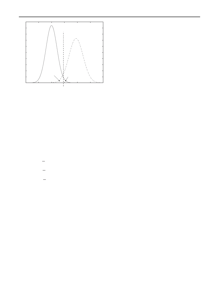
Fig. 1 Statistical model of antiviral detection

and in an antiviral detection context, if the null hypothe-
sis describes the fact that no infection occurred, the type
I error represents the false positive probability.

• the type II error β given by:

β = P[E ∈ A | H

1

true

] = P[e < S | H

1

true

],

In an antiviral context, it corresponds to the non-detec-
tion probability (if

H

0

is the non infection hypothesis).

These two different errors are described in Fig.

1

. It is essen-

tial to point out the fact that these two error risks are opposite
to one from the other. Indeed, each of them depends respec-
tively on A and A, whose disjoint union is

R. If we increase

the size of the acceptance region A, automatically that of
rejection region A decreases.

In most practical testings, the type I error is privileged.

Regions A and A are directly determined by it. Thus we
have to know the law of the null hypothesis. On the contrary,
the law of the alternative hypothesis is generally unknown.
That implies that determining the exact value of

β is most of

the time impossible.

To end with statistical testing, it is essential to stress on the

fact that error risks

α and β are, by definition never equal to

zero, except if the

H

0

and

H

1

probabilistic law domains (den-

sity functions) are disjoints. But in the latter case, it becomes
obvious that deciding is easy and that no testing is required
at all. From a practical point of view, our detailed analysis of
commercial antivirus [

5

] has shown that vendors generally

choose to minimize

α to the detriment of β.

3 Formal characterisation of antiviral detection

Let us now define our formal characterisation of virus
detection.

3.1 Definition of the model

A detection procedure D has to decide whether an input file

F is infected or not. For that purpose, D brings statistical

testing into play. As shown in [

5

], most of the time only one

is performed but as soon as viral techniques are becoming
more and more complex, antivirus should be forced to con-
sider several techniques (e.g. testings) at a time.

Let us assume that detector D performs n statistical tes-

tings

T

1

, . . . , T

n

. Without loss of generality we will consider

that these tests are applied sequentially, each of them apply-
ing to the results of the previous one. By definition, every of
these testing is marred by type I and II risks

α

i

and

β

i

.

Without loss of generality, we assume that the testings T

i

are independent one from each other. The result of

T

i

does

neither affect nor depend on that of

T

j

for i

= j. Let us then

state our first result.

Proposition 1 Let

n

independent

statistical

testings

T

1

, T

2

, . . . , T

n

, with respective type II error

β

i

. Then the

detection procedure D has residual non-detection probabil-
ity equal to

β =

n

i

=1

β

i

.

Proof It is sufficient to prove it for n

= 2. The equivalent

cumulated test

T

1

,2

will be considered with testing

T

3

and so

on.

Let us denote

H

i
0

and

H

i
1

the null and alternative hypoth-

eses respectively for the test

T

i

. The probability

β is then

defined by

β = P[non-detection|H

1

1

and

H

2

1

true

].

Under the assumption of independence, the alternative
hypotheses of

T

1

and

T

2

are independent too. We thus have:

β = P[non-detection|H

1

1

true

] × P[non-detection|H

2

1

true

].

and consequently

β = β

1

× β

2

.

Proposition

1

shows that if the non-detection probability

tends to zero, it cannot be equal to zero. Somehow, this is
a statitical variant of Cohen’s undecidability result. If a large
enough family of testings (with n

→ ∞), would result in

detecting with a null residual non-detection probability, this
would contradict Cohen’s result. As a consequence, as clearly
illustrated in Fig.

1

, the resulting false positive probability

123

68

E. Filiol, S. Josse

would be equal to one. Every possible file would be system-
atically and wrongly detected.

Remark In the general case, testing may be dependent. Then
β

1

will affect

β

2

and so on. But the previous result holds by

considering conditional probabilities. If we denote A

i

as the

event “non-detection occurs for test i ”, then

P

[A

1

A

2

A

3

. . . A

n

] = P[A

1

]P[A

2

|A

1

]P[A

3

|A

1

A

2

] . . .

×P[A

n

|A

1

A

2

. . . A

n

−1

].

As a general rule, the more testings are independent, the less
quickly

β tends to zero.

As far as false probability is concerned (risk

α), we can

state:

Proposition 2 Let

n

independent

statistical

testings

T

1

, T

2

, . . . , T

n

, with respective type I error α

i

. Then the

detection procedure D has residual false positive probability
equal to

α =

n

i

=1

α

i

.

Proof Let us prove for n

= 2. Let us assume that N files are

analyzed. Testing

T

1

wrongly detects in average

α

1

× N of

them. Testing

T

2

is then applied on those remaining files. By

definition, in average

α

1

× N ×α

2

files are wrongly detected.

Hence we have a residual

α = α

1

× α

2

.

The formal characterisation being defined, let us now precise
the two existing case: detecting known codes or know viral
techniques and detecting unknown codes using known viral
techniques.

3.2 Detection model for known alternative probabilistic law

The knowledge about the alternative law generally comes
from the malware analysis. The corresponding model is illus-
trated by Fig.

1

. In order to illustrate this case, let us consider

the didactic case of a trivial polymorphic technique: every

XOR Reg, Reg

is replaced with a

MOV Reg, 0

instruc-

tion (this is one of the rewriting rules in the metamorphic

Win32/MetaPHOR

engine).

Our sample will be made of N assembly instructions in

the code to be analysed. The estimator E measures the fre-
quency of the

MOV Reg, 0

instruction. Let us formulate

the null and alternative hypotheses. In a real context, they
will be defined through the statistical analysis of a large set
of uninfected files (

H

0

) and infected ones (

H

1

). We take the

theoretical mean value

µ of E as θ parameter.

Let us assume that under

H

0

the

MOV Reg, 0

appears

with probability p

0

. Thus, in average

1

µ = µ

0

= N × p

0

.

On the other hand, experiments have clearly shown that

for infected files, the

MOV Reg, 0

instruction occurs with

probability p

1

and thus

µ = µ

1

= N × p

1

. By defini-

tion, we have

µ

0

< µ

1

. We also know the standard devi-

ations (

σ

0

and

σ

1

) with respect to both hypotheses (

σ

i

=

√

N

× p

0

× (1 − p

0

)).

We thus have the following statistical testing:

H

0

: µ = µ

0

against

H

1

: µ = µ

1

.

We will choose

α = 0.05. Thus, in average 5% of the files

being analysed will be wrongly detected. As we assume to
known the alternative law, we can fix

β = 0, 01. This means

that we do not accept that more than 1% of the infected files
remain undetected.

Since the central limit theorem applies (N

> 30), we will

use the normal distribution as an approximation of the prob-
abilistic law of

θ = µ (otherwise we would use the Student

law). Thus under

H

0

, then E follows the

N (µ

0

, σ

0

) whereas

under

H

1

, it is distributed according to

N (µ

1

, σ

1

).

All things being now defined, it is somehow easy yet tricky

to compute the decision threshold S. Basic calculus tech-
niques (see [

7

] for the details) give:

Nmin =

b

√

p

1

q

1

− a√p

0

q

0

p

0

− p

1

2

,

S

= N p

0

+ a

N p

0

q

0

= N p

1

+ a

N p

1

q

1

where q

i

= 1− p

i

and, with

(.) denoting the normal cumu-

lative density function,

a

=

−1

(α)

b

=

−1

(β)

The value Nmin is the minimum value that N (the number
of instructions in the code) must have so that our statistical
model holds. Otherwise we would either have to consider
another estimator or modify the risk values.

The decision rule is then straightforward. Suppose that

E

= e with respect to the file being analysed, we have:

1

We will use in a first approach that each instruction is a Bernoulli

variable, with the successful event being defined as “is equal to

MOV

Reg, 0

”. Despite the fact that instructions in the code are not really

independent (it is in fact a Markov) process, we will approximate as
they would be. Simulations have shown that this approximation is good
enough to describe things while keeping the model simple enough.

123

A statistical model for undecidable viral detection

69

if

e

− µ

0

σ

0

<

S

− µ

0

σ

0

, we cannot reject

H

0

,

the file is likely to be non infected

,

otherwise

, we reject

H

0

,

the file is likely to be infected.

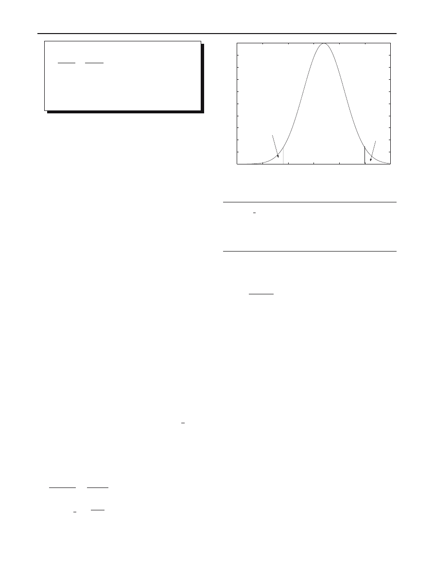
3.3 Detection model for unknown alternative probabilistic

law

This case refers to the detection of unknown codes that
nonetheless use known viral techniques. Thus, we know the
null hypothesis only:

H

0

: θ = θ

0

.

We can perform any of the three hypothesis testing:

H

1

: θ > θ

0

H

1

: θ < θ

0

H

1

: θ = θ

0

We will consider the last two-sided test which is the most
general one (we do not any assumption on the value

θ com-

pared to the value

θ

0

).

Let us consider the estimator E for the appearance fre-

quency of the instruction

XOR Reg, Reg

in uninfected

files. We state the null hypothesis as

H

0

: µ = µ

0

. Since

many polymorphic/metamorphic techniques use rewriting
techniques [

7

], it is likely that in infected files

µ

0

may either

decrease (when replaced by the

MOV Reg, 0

instruction)

or increase (when using garbage code). So we state the alter-
mative hypothesis as

H

1

: µ = µ

0

.

As in the previous section, we assume that

H

0

has the

normal distribution

N (µ

0

, σ

0

). The testing is built in the

same way as before. We fix

α = 0, 05 (as an example). This

corresponds to the rejection region that is divided into two
equal parts (recall the test is two-sided; see Fig.

2

), each of

them referring to a rejection probability equal to

α

2

. But the

essential difference with the previous testing lies in the fact
that we cannot bring the risk

β under control and thus infer

the corresponding non-detection probability with respect to
the present testing. Consequently, the decision threshold S is
such that

P

|E − µ

0

|

σ

0

>

S

− µ

0

σ

0

= α.

The value z

α

2

=

S

−µ

0

σ

0

is given by the normal cumulative

density function.

−15

−10

−5

0

5

10

15

0

0.01

0.02

0.03

0.04

0.05

0.06

0.07

0.08

0.09

0.1

H

0

→

α/2

α/2

Fig. 2 Statistical model of unknown viruses detection

Table 2 Decision rule for unknown viruses detection testings

if R.C.

< z

α

2

, we cannot reject

H

0

,

the file is likely to be uninfected

,

otherwise

, we reject

H

0

,

the file is likely to be infected

.

Finally, if E

= e on the code being analysed, we compute

the critical ratio:

R.C.

=

|e − µ

0

|

σ

0

.

The decision rule is then given in Table

2

. This kind of testing

enables to consider a file as a suspect one (

H

0

is rejected).

Consequently the file will be systematically disassembled
in order to confirm its true nature (infected or not). On the
contrary, we cannot have any insight on the non-detection
probability. The present model clearly explains why.

4 Antiviral detection techniques and statistical testing

Let us now explain how classical antiviral detection tech-
niques can be modeled as statistical testings.

4.1 Classical signature-based detection

Most of the time, antivirus software heavily relies on pat-
tern detection techniques [

5

]. In other words, for a mal-

ware

M, they look for a fixed sequence of bytes σ

M

∈

{0, 1, 2, . . . , 255}

s

with s

= |σ

M

|.

Let us consider a file F to be analyzed by means of a

detector D. We then model this technique by considering that
most of the pattern search algorithms (Rabin–Karp algorithm
[

9

], finite automaton search [

1

], Knuth–Morris–Pratt method

[

10

], Boyer–Moore algorithm [

2

]...) evaluate a large number

123

70

E. Filiol, S. Josse

of s-byte subsets in F , before to eventually find the suitable
viral pattern.

The search for a viral pattern

σ

M

may be described by

a sum of Bernoulli trials. We define the following Bernoulli
variable

2

with respect to a subset

S

i

of bytes of size s (non

necessary contiguous) in F .

X

S

i

=

S

i

= σ

M

p

0

S

i

= σ

M

q

0

= 1 − p

0

The value p

0

is directly determined by its efficiency as defined

in [

5

]. If the file F contains n bytes, there are at most N

=

n

s

possible s-byte subsets in F . Then we define the following
estimator:

Z

=

S

i

∈

P(F),|S

i

|=s

X

S

i

.

Then the null hypothesis

H

0

states that F is not infected. The

relevant probabilistic law is the normal distribution
N (N.p

0

,

√

N p

0

q

0

). The alternative hypothesis H

1

is very

simple to determine. We indeed have

H

1

: µ = 1. If the file F

is infected, the detector will terminate as soon as it has found
the viral pattern

σ

M

. Consequently, we can describe the

“law” of

H

1

by the density function f

(1) = 1 and f (x) = 0

whenever x

= 1. Then µ

1

= 1 and σ

1

= 0.

Let us recall that only two cases may occur:

• the file F is infected by the malware M, so we have

µ = µ

1

= 1 (with a probability which is equal to 1);

• the file F is infected by a malware M

which is not

recorded in the viral database yet. Then, with respect to
σ

M

, we have

µ = µ

0

.

The corresponding statistical testing is then simple to set up.
For a fixed

α, we compute z

α

2

and R.C as shown in the previ-

ous section (case of unknown alternative probabilistic laws).
Finally the suitable decision rule is applied. From a practical
point of view, as soon as n and s are large enough, an empiric
threshold equal to 1 can be used.

Here computing the non-detection probability

β is non

sensical. If the file F is infected by the malware

M for which

the viral database has been updated, the probability P

[Z <

1

|H

1

true

] = 0 with respect to M. Indeed, we have P[Z ≥

1

|H

1

true

] = 1. If the code is a known one, it will be system-

atically detected. Consequently, to evaluate the non-detection
probability as far as signature-based detection is concerned,
we must not do it with respect to a given malware. In this
respect, we can define the non-detection probability as

2

In a first approach, this approximation holds since no particular

assumption is done about files F to be analysed. Thus they may be
considered a priori as containing random data.

follows:

P

[non-detection] =

|B

D

|

ℵ

0

=

|B

D

|

∞

→ 0,

where

B

D

describes the viral database used by detector D

and where

ℵ

0

denotes the total number of possible viruses

[

4

, Chap. 3].

4.2 The general case of detection scheme or detection

strategies

Detection schemes [

5

] with respect to a given malware

M is

a pair

{S

M

, f

M

} where S

M

is the detection pattern and f

M

is the detection function. The concept of detection strategies
[

6

] generalizes that of detection scheme by considering a trip-

let

DS = {S

M

, B

M

, f

M

} which additionally includes a set

B

M

of program functions (behaviors). It has been proved that

whereas detection scheme models every possible sequence-
based detection techniques [

5

], detection strategies models

general detection [

6

], whatever techniques is considered –

sequence-based and/or behavior-based.

In this general context, the previous statistical model fully

applies. The essential difference lies in the fact that the detec-
tion function has a weight which is strictly greater than
1—simple signature based detection considers detection
function which has a weight strictly equal to 1.

Let us note

ω = wt( f ), the expected probability p

0

equals

ω

256

s

instead of

1

256

s

. Consequently the false positive proba-

bility increases, but most of the time it remains negligible.

4.3 Other cases

For a number of (exotic) detection techniques, the detection
function is too complex to be considered. As a consequence,
stating the null hypothesis is practically untractable and the
exact distribution law cannot be determined. An empiric law
is then to be considered instead, which can be tuned up
according a posteriori knowledge (Bayesian approach).

The authors of new techniques generally give experimen-

tal results as far as risks

α and β are concerned. As an exam-

ple, self-organizing map-based detection technique, which
has been proposed by I. Yoo and U. Ultes-Nitsche [

13

], yields

α = 0, 3 and β = 0, 16. Every new technique proposed
should be systematically published with those experimental
risk values along with all relevant data that would help to
reproduce that technique.

Due to lack of space, we will not go deal with heuris-

tics [

11

,

12

] or meta-heuristics like tabu search, greedy algo-

rithms, simulated annealing... From a general point of view,
we have shown in [

7

] that any heuristic or meta-heuristics

can be translated in terms of statistical tests. Consequently,
all previous results hold for these particular detection
techniques.

123

A statistical model for undecidable viral detection

71

5 Statistical testing simulability: defeating antiviral

detection

Our formal characterization of antiviral detection clearly
enables us to precisely identified why and how these tech-
niques have inherent limitations. But beyond the intrinsic risk
of wrong decisions, there exist a much worse situation: when
the attacker use the detection techniques against the defender.
As soon as the first one knows which tools are used by the
second, he is able to perform what we call statistical testing
simulability.

Let us give a definition for this concept.

Definition 1 Simulating a statistical testing consists for an
adversary, to introduce, in a given population

P, a statistical

bias that cannot be detected by an analyst by means of this
test.

There exist two different kinds of simulability:

• the first one does not depend on the testings (and their

parameters) the defender usually considers. It is called
strong testing simulability.

• on the contrary, the second one does depend on those

testings that the attackers aims at simulating. It is called
weak testing simulability.

In this section, we call “tester” the one who uses statistical
testing in order to decide.

5.1 Strong testing simulability

Let us define this concept more precisely.

Definition 2 (Strong testing simulability) Let P be a prop-
erty and T a testing whose role is to decide whether P holds
for given population

P. Strongly simulating this testing con-

sists in modifying or building a biased population P in such
a way that T systematically decides that P holds on

P, up

to the statistical risks. But there exists a statistical testing T

which is able to detect that bias in

P. In the same way, we

say that t testings

(T

1

, T

2

, . . . , T

t

) are strongly simulated, if

applying them results in deciding that P holds on

P but does

no longer hold when considering a

(t + 1)-th testing T

t

+1

.

In terms of security, strong simulability is a critical aspect
in security analysis. Many applications have been identified,
especially in cryptography [

7

]. In an antiviral context, strong

simulability exist when the malware writer, who has iden-
tified any of the techniques used by one or more antivirus,
writes malware that cannot be detected by the target antivi-
rus but only by the malware writer. As a typical example, a
viral database which contains t signatures is equivalent to t
testings (see previous section) and any new malware corre-
sponds to the testing T

t

+1

.

5.2 Weak testing simulability

Let us define this concept more precisely.

Definition 3 (Weak testing simulability) Let P be a property
and T a testing whose role is to decide whether P is valid for
a given population

P or not. To weakly simulate this testing

means introducing in

P a new property P

which partially

modifies the property P, in such a way that T systematically
decides that P holds on

P, up to the error risks.

Weak simulability differs from strong simulability since the
attacker considers the same testings as the tester. The attacker
thus introduces a bias that the tester used will not be able to
detect.

The property P

of Definition

3

is generally opposite to

the property P. It precisely represents a flaw that the attacker
aims at exploiting. Bringing weak simulability into play is
somehow tricky. It requires to get a deep knowledge of the
testings to be simulated.

The central approach consists in introducing the property

P

in such a way that the estimators E

i

in use remain in the

acceptance region of the testing (generally that of the null
hypothesis). Let us recall that during the decision step, the
tester checks whether E

< S or not. Thus weak simulabil-

ity consists in changing the value S

− E while keeping it

positive. For that purpose, we use the intrinsic properties of
the relevant sampling distribution.

5.3 Application: defeating detection

Many applications of testing simulability have been imag-
ined [

7

]:

• bypassing stream filtering (e.g. to detect the spread of

worms);

• bypassing data filtering (e.g. blocking of encrypted or

zipped data);

• defeating antiviral detection.

Let us present a detailed case with respect to the last point.
It is essential to point out that simulability is done by the
attacker once and for all. Indeed, antivirus publishers do not
change the underlying statistical model of their products very
often. Without loss of generality, we will consider the case
of spectral analysis which seems the more tricky to simu-
late since the underlying detection function is too complex
to represent.

Let us recall that spectral analysis [

4

] consists in listing

some critical instructions of the code. This list is called the
spectrum. Every compiler used a small subset only of all pos-
sible intructions. On the contrary, a malware will consider the
whole set of these instructions.

123

72

E. Filiol, S. Josse

Let us consider a spectrum with respect to a given compiler

C made of a list of instructions (I

i

)

1

≤i≤c

, each of them along

with its expected frequency n

i

(in uninfected programs). The

spectrum is thus given by:

spec

j

(C) = (I

i

, n

i

)

1

≤i≤c

.

The index j means that in practice we may consider more
than one spectrum. Without loss of generality, we will con-
sider only one.

Whenever a program is analysed by the detector, the

observed frequencies

ˆn

i

are recorded. The null hypothesis

H

0

is the statement:

H

0

: ˆn

i

= n

i

1

≤ i ≤ c.

The alternative hypothesis

H

1

consists in claiming that the

spectrum of the program being analysed significantly differs
from the expected one and thus the program is likely to be
infected.

We use then the estimator

D

2

=

c

i

=1

(ˆn

i

− n

i

)

2

n

i

.

It is a well-known fact that D

2

asymptotically has a

χ

2

distri-

bution with c

− 1 degrees of freedom, under the assumption

that

H

0

holds. For a fixed type I error

α, the decision step

consists in comparing the value of estimator D

2

with the

decision threshold

χ

2

(α,c−1)

. We then decide:

H

0

if D

2

≤ χ

2

(α,c−1)

H

1

if D

2

> χ

2

(α,c−1)

.

Let us now explain how to simulate this testing. Let us assume
that during a metamorphic process in a malware, rewriting
techniques have been used. They are likely to modify the
expected frequency n

i

in the reference spectrum. The meta-

morphic engine generally considers random rewriting rules
[

7

]. But how random must be the rules in order to not trigger

any alert when the file is analysed?

Without loss of generality and for the sake of clarity, let us

consider that only two instructions I

i

1

and I

i

2

of the spectrum

have been rewritten. Let us explain how the metamorphic
engine will have to tune up its mutations in order to weaky
simulate spectral analysis.

Instructions I

i

1

and I

i

2

have expected frequency n

i

1

and

n

i

2

respectively. Let us first consider the initial code (variant

at time t

= 0). It is such that

D

2

=

c

i

=1

(ˆn

i

− n

i

)

2

n

i

≤ χ

2

(α,c−1)

,

(1)

with respect to a given type I error

α. The corresponding

initial (reference) value of D

2

is denoted D

2

0

and we denote

F

= χ

2

(α,c−1)

− D

2

.

Then the metamorphic process modifies frequency

ˆn

i

1

and

ˆn

i

2

as follows:

ˆn

i

1

→ ˆn

i

1

ˆn

i

1

+ δ

1

= ˆn

i

1

(2)

ˆn

i

2

→ ˆn

i

2

ˆn

i

2

+ δ

2

= ˆn

i

2

(3)

Values

δ

i

may be negative or positive. In a first approach, it

is obvious that a first criterion is to make sure that E

[δ

1

+

δ

2

] = 0 (the mathematical mean of instruction modifications

is equal to 0). But this criterion is rather restrictive and the
number of mutation possibilities will be limited. Moreover,
this criterion depends on the initial code only and not on the
expected frequencies n

i

. Let us consider a more general and

more powerful criterion.

Copying out the modifications of

ˆn

i

1

and

ˆn

i

2

in Equa-

tion (

1

), we can write

D

2

=

c

i

=1,i∈{i

1

,i

2

}

(ˆn

i

− n

i

)

2

n

i

+

(ˆn

i

1

− n

i

1

)

2

n

i

1

+

(ˆn

i

2

− n

i

2

)

2

n

i

2

.

(4)

This enables to come back to the value D

2

0

, when taking

Equations (

2

) and (

3

) into account:

D

2

= D

2

0

+

2

δ

1

(ˆn

i

1

− n

i

1

) + δ

2

1

n

i

1

+

2

δ

2

(ˆn

i

2

− n

i

2

) + δ

2

2

n

i

2

. (5)

Equation (

5

) thus gives the criterion we are looking for:

E

2

δ

1

(ˆn

i

1

− n

i

1

) + δ

2

1

n

i

1

+

2

δ

2

(ˆn

i

2

− n

i

2

) + δ

2

2

n

i

2

= 0. (6)

or equivalently

E

[2δ

1

(ˆn

i

1

−n

i

1

)n

i

2

+δ

2

1

n

i

2

+2δ

2

(ˆn

i

2

−n

i

2

)n

i

1

+δ

2

2

n

i

1

] = 0.

(7)

A quick analysis shows that this criterion is far less restrictive
that the first one (E

[δ

1

+ δ

2

] = 0).

The polymorphic engine has thus to randomly modify

instructions I

i

1

and I

i

2

in such a way that frequencies

ˆn

i

1

and

ˆn

i

2

keep on verifying the criterion stated by Equation (

7

).

This simulability scheme can be generalised further. We

only considered here a didactic, simple scenario. Let us give
some more sophisticated mechanisms:

• the criterion of Equation (

7

), from a practical point of

view, must be brought into play along with the variance
given by

=2δ

1

(ˆn

i

1

− n

i

1

)n

i

2

+δ

2

1

n

i

2

+2δ

2

(ˆn

i

2

− n

i

2

)n

i

1

+δ

2

2

n

i

1

.

123

A statistical model for undecidable viral detection

73

Indeed, weak simulability practically requires that

D

2

0

+ < χ

2

(α,c−1)

,

or equivalently that

< F. If we would take the value

E

[] only into account, with a non null probability, the

value

χ

2

(α,c−1)

may be too large thus resulting in rejecting

H

0

. We thus are forced to consider the variance (in other

words the mean behaviour of the deviations with respect
to E

[]);

• it is powerful to consider a large enough spectrum, Indeed

it allows to create fake instructions modifications that can
balance other useful or compulsory modifications. It is
thus easier for the estimator to remain in the acceptance
region;

• the value , when generalised to a larger spectrum, can

also have a negative statistical mean (

−D

2

0

≤ ≤ F).

This increases the power of weak simulability .

6 A statistical variant of Cohen’s undecidability

We have proved with Proposition

1

that non-detection prob-

ability cannot be equal to 0 in any way. This result represents
somehow a statistical formalisation Cohen’s undecidability
[

3

]. Indeed, if a finite enumerably set of statistical tests would

cancel the non-detection probability, thus we would obtain a
result that contradicts Cohen’s one. As far as false positive
probability is concerned, according to Fig.

1

, it would equal

exactly one. In other words, we would detect any file submit-
ted to detection as infected.

The concept of test simulability enables us to give an illus-

tration of the undecidable antiviral detection which is a sta-
tistical equivalent to Cohen’s famous algorithmic example
called contradictory virus (C V ). Let us consider a detection
procedure D which is able to distinguish a virus V from any
other program. Its pseudo-code is given by:

CV() {

......

main() {

if not D(CV) then {

spread();

if trigger_condition is true then payload();

}

End if

Go to next target program

}}

F. Cohen has proved that D did not exist and that any

detection based on D is undecidable.

According to our statitical model of detection and to the

concept of statistical simulability we have developed, the
virus C V may be reformulated as follows. The detection pro-
cedure D is made of n statistical tests

T

1

, T

2

, . . . , T

n

. Then,

C V ’s pseudo-code is given by:

CV() {

......

simul(D, V) {

generate V’ by (statistically) simulating D from V

return V’

}

main() {

if not D(CV) then {

spread();

if trigger_condition is true then payload();

}

else

{

V’ = simul(D, CV)

run V’

}

End if

Go to next target program

} }

Thus, D is a contradictory procedure as well:

• If D decides that CV is a virus, then CV mutates by

simulating tests

T

1

, T

2

, . . . , T

n

in D.

• On the other hand, if D decides conversely (CV is not a

virus), the infection occurs and C V is indeed a virus.

7 Future work and conclusion

In this paper we have presented the formal characterisation of
antiviral detection. We thus are able to understand why anti-
virus software have a limited efficiency by nature but how an
attacker can exploit antivirus intrinsic limitations. In particu-
lar, this model clearly shows that antivirus efficiency directly
depends on the antivirus publishers’ strategic choices: either
lowering false positive probability (but increasing non-detec-
tion probability) or lowering non-detection probability (but
increasing false positive probability).

Future work addresses the problem of finding more pow-

erful statistical testings scheme that:

• succeeds in lowering as much as possible the type II

error with a number of testings which is as much reduced
as possible. An interesting trend could be to characte-
rise uninfected programs (thus the null hypothesis) on a
more combinatorial basis (e.g use of randomized design,
design of experiments);

• and hinders as much as possible testing simulability.

Testing simulability clearly shows that whenever an attacker
knows all the detection techniques which are used by an
antivirus software, he is able to bypass and to defeat it. This
fact strongly militates against detection scheme extraction
capabilities of the attacker. Then secure detection scheme
as proposed in [

5

] should be systematically considered and

implemented in antivirus software to hinder or even forbid
test simulability and thus the ability by attacker to bypass
antiviral detection.

123

74

E. Filiol, S. Josse

References

1. Aho, A.V., Hopcroft, J.E., et Ulman, J.D.: The Design and Analysis

of Computer Algorithms. Addison-Wesley, Reading (1974)

2. Boyer, R.S., et Moore, J.S.: A fast string-searching algo-

rithm. Commun ACM 10(20), 762–772 (1977)

3. Cohen, F.: Computer viruses. Ph.D. Thesis, University of Southern

California, Janvier (1986)

4. Filiol, E.: Computer Viruses: from Theory to Applications,

IRIS International Series, Springer, France. ISBN 2-287-23939-
1 (2005)

5. Filiol, E.: Malware pattern scanning schemes secure against black-

box analysis. In: Broucek, V., Turner, P. (eds.) EICAR Confer-
ence Best Paper Proceedings, Hamburg, Germany: EICAR. An
extended version has been published in the EICAR 2006 Special
Issue, J. Comput. Virol. 2(1), pp. 35–50 (2006)

6. Filiol, E., Jacob, G., Le Liard, M.: Evaluation methodology and

theoretical model for antiviral behavioural detection strategies. In:
Bonfante, G., Marion, J.-Y. (eds) WTCV’06 Special Issue, J. Com-
put. Virol. 3(1) (2007)

7. Filiol, E.: Techniques virales avancées, IRIS Series, Springer,

France. An English translation is pending (due mid 2007) (2007)

8. Chess, D.M., White, S.R.: An undetectable computer virus. In:

Virus Bulletin Conference (2000)

9. Karp, R.M., et Rabin, M.O.: Efficient Randomized Pattern-Match-

ing Algorithms, Technical report TR-31-81. Ayken Computation
Laboratory, Harvard University (1981)

10. Knuth, D.E., Morris, J.H., et Pratt, V.R., Jr.: Fast pattern-matching

in strings. SIAM J. Comput. 2(6):323–350 (1977)

11. Schmall, M.: Heuristische Viruserkennung. Diplom Thesis, Uni-

versität Hamburg (1998)

12. Schmall, M.: Classification and identification of malicious code

based on heuristic techniques utilizing Meta languages. Ph.D.
Thesis, University of Hamburg (2003)

13. Yoo, I., Ultes-Nitsche, U.: Non-signature-based virus detection:

towards establishing unknown virus detection technique using
SOM. J. Comput. Virol. 3(2), 163–186 (2006)

123