arXiv:math-ph/0112059 v1 30 Dec 2001
Preprint LEEDS-MATH-PURE-2002-01
arXiv:math/0112059
, 2001
Meeting Descartes and Klein
Somewhere in a Noncommutative Space
Vladimir V. Kisil
Abstract. We combine the coordinate method and Erlangen program in the
framework of noncommutative geometry through an investigation of symme-
tries of noncommutative coordinate algebras. As the model we use the coher-
ent states construction and the wavelet transform in functional spaces. New
examples are a three dimensional spectrum of a non-normal matrix and a
quantisation procedure from symplectomorphisms.
Contents
1
2. Descartes Meets Klein: Symmetries of Coordinate Algebras
2
3. Coherent States and Wavelets in Mathematics and Physics
4
4. Functional Calculus as an Intertwining Operator
16
5. Quantisation from the Symplectic Invariance
19
23
23
23
1. Introduction
Mathematics is a part of physics. Physics is an experimen-
tal science, a part of natural science. Mathematics is the
part of physics where experiments are cheap.
Vladimir Arnold [3]
We used to think by a small number of mental images which help us to under-
stand equally good (or bad) a variety of different processes. A “Big Bang” is one of
such pet ideas which we call archetypes to excuse their overloading. K. Jaspers
1991 Mathematics Subject Classification. Primary: 43A85; Secondary: 30G30, 42C40,
46H30, 47A13, 81R30, 81R60.
Key words and phrases. Heisenberg group, special linear group, symplectic group, Hardy
space, Segal-Bargmann space, Clifford algebra, Cauchy-Riemann-Dirac operator, M¨
obius trans-
formations, functional calculus, Weyl calculus (quantization), quantum mechanics, Schr¨
odinger
representation, metaplectic representation.
On leave from the Odessa University.
c
0000 (copyright holder)
1

2
VLADIMIR V. KISIL
argued that modern culture appeared from a black matter as result of a big bang
at the axial period more than two thousand years ago. The expanding Universe
of human culture became split into many seemingly independent galaxies—science,
religion, art, etc.—each with its own complicated structure and dynamics. The
cosmological belief that all future of a Universe was determined by the first min-
utes after the bang may not be true but has an appeal of simplicity. Anyway it is
natural to expect that after the bang all parts will run away each other. Thus the
appearance of two cultures in the sense of C.P. Snow, which are disjoint or even
in an opposition, seems to be unavoidable.
Yet there is also another persistent pattern: mathematics since Elements of
Euclid grown enormously both in qualitative and quantitative sense but did not
split into several smaller independent subjects. And the border between mathe-
matics and physics (if ever exists at all) is as thin today as in times of Archimedes.
Moreover a smuggling across that border in both direction is more rewarding today
than ever before. Is there a hidden rules or forces which tie them together despite
of general centrifugal tendencies?
2. Descartes Meets Klein: Symmetries of Coordinate Algebras
If you would be a real seeker after truth, you must at least
once in your life doubt, as far as possible, all things.
Descartes Discours de la M´
ethode, 1637
The striking example of centripetal trends in mathematics is the Cartesian
coordinate method. Before the XVII century there were two big and relatively in-
dependent mathematical subjects with different (even geographically) origins: the
synthetic geometry of Greeks and abstract algebra of Arabs. It was natural to ex-
pect that these fields will diverge even further during their developments. Thus the
proposition of Descartes to associate geometrical problems with algebraic equa-
tions by an introduction of coordinates was a great manifestation of the integrity of
mathematics. Another example of unexpected links between seemingly unrelated
topics was the Galois discovery that solvability of algebraic equations depends on
certain group-theoretic properties of their Galois group. Just putting together these
two ideas one may suspect that there is a connection between geometry and group
theory. That connection was announced in the famous Erlangen program of Felix
Klein developed under the strong influence of Sophus Lie: synthesis of geometry
as the study of the properties of a space that are invariant under a given group of
transformations.
We will not retell once again the story of coordinate approach in noncommu-
tative spaces, see for example [41] for a balanced and concise exposition. Instead
we would highlight few observations oftenly overlooked in the current literature:
(1) The rule that coordinates should form an algebra was not introduced by
Descartes originally, it is sufficient that coordinates have any rich alge-
braic structure to reflect all geometrical properties, for example, via alge-
braic or differential equations. The identification
coordinates = anassociativealgebra + sometopology
(2.1)
was fixed only after the Gelfand theory of commutative Banach algebras.
While the achievements based on (2.1) are really impressive [11] that iden-
tification is not necessary (see bellow) and could be a needless restriction
in general.
DESCARTES AND KLEIN ON NONCOMMUTATIVE GEOMETRY
3
(2) The development of noncommutative geometry was oftenly motivated and
supported by the representation theory of groups. For example, the origi-
nal paper on noncommutative measure and integration theory [37] leaded
to the Plancherel theorem for noncommutative locally compact groups.
Quantum theory—the stronghold of Cartesian approach to noncommuta-
tive spaces—was able to deal with elementary particles or four basic inter-
actions only in the Erlangen spirit through their symmetry groups.
(3) The Cartesian connection of geometrical problems with algebraic equa-
tions was not a subordination of geometry to algebra, actually Descartes
used it in both ways and introduced a geometrical method for solutions of
quadratic equations. Forever geometry be seen as an extremely beautiful
subject with its own charm: “a geometrical proofs” usually means “an el-
egant proof”, and its is fashionable to say “I am doing noncommutative
geometry” rather than “I am studying operator algebras and applications”.
We challenge the rigid identification (2.1) in this paper and use the assumption:
coordinates are oftenly a representation space for a group action
(2.2)
to approach certain problem in noncommutative spaces. The fact that sometimes
coordinates form also an algebra could be useful but is not crucial anymore. We
will see in the last two sections that it is even helpful to downplay the structure
of algebras by abandoning the algebraic homomorphism property. The number of
applications is not limited to given in the present paper, (see in addition Example 2
in [24] with the Manin plane and quantum groups [32]) and they deserve a further
investigation.
One can object [11] that homogeneous spaces which are geometries in the sense
of the Klein program are too restrictive to give a good model of space-time in general
relativity. There is no a hard evidence to refute that claim at the moment, but we
could learn from the inspiring paper [8] that symmetries of objects are usually
richer than people ordinary think. For example, even the structure of a single point
could be significantly enriched by introduction of a coordinate bundle over it [8,
§ 6] and assigning a group action in that bundle. Therefore one could make the
following conjecture, which we illustrate by examples in the present paper.
Conjecture 2.1. The combination of Cartesian and Klein-Lie approaches
based on the assumption (2.2) is stronger than the original Erlangen program itself
and could go beyond previous limits.
The rest of the paper is organised as follows. In the next Section we will study
symmetries of functional spaces which are coordinates in commutative cases. This
will be our platform for an invasion to noncommutative spaces, similarly to the
Gelfand structural theorem about commutative Banach algebras in the approach
based on identification (2.1). The technique is widely known as coherent states con-
struction and wavelet transform but was rediscovered many times before and after
those names were coined. We show that many fundamental notions of analysis are
intimately connected to that circle of ideas, which are yet not explicitly understood
and used to its full power.
Intertwining commutative and noncommutative coordinates in Section 4 we will
get a new description of functional calculus and related spectrum of non-normal
matrices. The calculus and the spectrum are naturally connected through an ap-
propriately extended spectral mapping theorem.
4
VLADIMIR V. KISIL
We also approach the quantisation problem with the similar ideas in Section 5
and get a natural combination of quantum and classical mechanics within the frame-
work of the Heisenberg group.
This paper is a survey or even an essay on the subject. The three main sections
are rather connected by a common idea than technically dependent. Therefore they
could be looked through almost separately. More details could be found in published
papers [22, 23, 25, 27] and will also appear in [26, 28].
3. Coherent States and Wavelets in Mathematics and Physics
In the 1960’s it was said (in a certain connection) that the
most important discovery of recent years in physics was the
complex numbers.
Yu.I. Manin [31, Preface]
We would like to present a construction which produces many important objects
in analytic function theory, i.e. commutative coordinate spaces, out of symmetry
groups. The scheme is well known, cf. [1, 34] and got much attention in recent
decades but it is not used to its full potential yet. Our main examples are pro-
vided by the one dimensional Heisenberg group
H = H
1
2
(
R)
groups [19, 30, 44]—two groups with the outmost importance [18, 19] in both
mathematics and physics.
The one dimensional Heisenberg group
H consists of points (s, z) = (s, x, y)
parametrised by s
∈ R and z = x + iy ∈ C. The group law is given by:
g
∗ g
0
= (s, z)
∗ (s
0
, z
0
) = (s + s
0
+
1
2
=(¯zz
0
), z + z
0
),
(3.1)
where
=w denotes the imaginary part of a complex number w. The H is the
necessary component (sometimes implicit) of any quantisation scheme because its
Lie algebra has the only non-trivial commutator:
[][X, Y ] = S,
which in the Shr¨
odinger representation (see bellow (3.17)) takes a form of the
celebrated Heisenberg uncertainty relation.
The group SL
2
(
R) consists of 2 × 2 matrices
a
b
c
d
with real entries and
determinant ad
− bc = 1. Its is also isomorphic to the following three groups [44,
§ 8.1] which wee will use bellow in different contexts:
(1) the Lorentz type group SO
e
(1, 1) in the two-dimensional Minkowski space
with the metric ds
2
= dt
2
− dx
2
;
(2) the group SU (1, 1) of linear transformation of
C
2
preserving the quadratic
form z
2
1
− z
2
2
;
(3) the symplectic group Sp(1) of linear symplectomorphisms of the two di-
mensional flat phase space in classical mechanics.
It is not surprising that
H and SL
2
(
R) are intimately connected to each other
as we will see and use in the Section 5.
3.1. Space-Time or Phase Space from Symmetry Groups. There is a
heuristic observation [41] that a space-time is not a primary concept but appears in
the approach based on the identification (2.1) as the spectrum of a maximal com-
mutative subalgebra of the algebra of observables invariant under the fundamental
group. We show in this subsection that simplest forms of the space-time and the
DESCARTES AND KLEIN ON NONCOMMUTATIVE GEOMETRY
5
phase space could be naturally obtained just from symmetry groups in the context
of (2.2). It is interesting to note that the same group could produce several rather
distinct spaces, e.g. with elliptic or hyperbolic metrics.
Abstract scheme could be described as follows. Let G be a group and H be its
closed normal subgroup, which could be trivially just
{e}. Let X = G/H be the
corresponding homogeneous space with an invariant measure dµ and s : X
→ G be
a Borel section in the principal bundle G
→ G/H [21, § 13.2]. Then any g ∈ G has
a unique decomposition of the form g = s(x)h, x
∈ X and we will write x = s
−1
(g),
h = r(g) = (s
−1
(g))
−1
g. Note that X is a left G-homogeneous space with an action
defined in terms of s as follow:
g : x
7→ g · x = s
−1
(g
−1
∗ s(x))
(3.2)
where
∗ is the multiplication on G.
We will illustrate our consideration by a chain of examples. Each one consists
of four parts numbered from (a) to (d): two cases for G =
H with two different
subgroups H =
R
2
and H =
R, see [25] for more details; other two cases for
G = SL
2
(
R) with subgroup H = K and H = A studied in [23].
Example 3.1. (a) We start from
H and its subgroup H = R
2
=
{(t, z) |
=(z) = 0}. Then X = G/H = R and because the Haar measure on H coincides
with the standard Lebesgue measure on
R
3
§ 1.1] then invariant measure on X
coincides with the Lebesgue measure on
R. Mappings s : R → H and r : H → H
are defined by the identities s(x) = (0, ix), s
−1
(t, z) =
=z, r(t, u + iv) = (t, u). The
composition law s
−1
((t, z)
· s(x)) = x + u reduces to Euclidean shifts on R. We also
find s
−1
((s(x
1
))
−1
· s(x
2
)) = x
2
− x
1
and r((s(x
1
))
−1
· s(x
2
)) = 0. This X is the
configuration space of a particle with one degree of freedom.
(b) As a subgroup H =
R we select now the one dimensional centre of H consisting
of elements (s, 0). Of course X = G/H isomorphic to
C and mapping s : C → G
simply is defined as s(z) = (0, z). The invariant measure on X also coincides
with the Lebesgue measure on
C. Note also that composition law s
−1
(g
· s(z))
reduces to Euclidean shifts on
C. We also find s
−1
((s(z
1
))
−1
· s(z
2
)) = z
2
− z
1
and
r((s(z
1
))
−1
· s(z
2
)) =
1
2
=¯z
1
z
2
–the symplectic form on
R
2
. In that case we get the
phase space of a particle with one degree of freedom.
(c) Here we study SL
2
(
R) in the form of the group SU(1, 1) of 2 × 2 matrices with
complex entries of the form
α
β
¯
β
¯
α
such that
|α|
2
− |β|
2
= 1. SL
2
(
R) has the
only non-trivial compact closed subgroup K, namely the group of matrices of the
form h
ψ
=
e
iψ
0
0
e
−iψ
. Any g
∈ SL
2
(
R) has a unique decomposition of the
form
α
β
¯
β
¯
α
=
1
q
1
− |a|
2
1
a
¯
a
1
e
iψ
0
0
e
−iψ
(3.3)
where ψ =
= ln α, a = β ¯
α
−1
, and
|a| < 1 because |α|
2
− |β|
2
= 1. Thus we
can identify SL
2
(
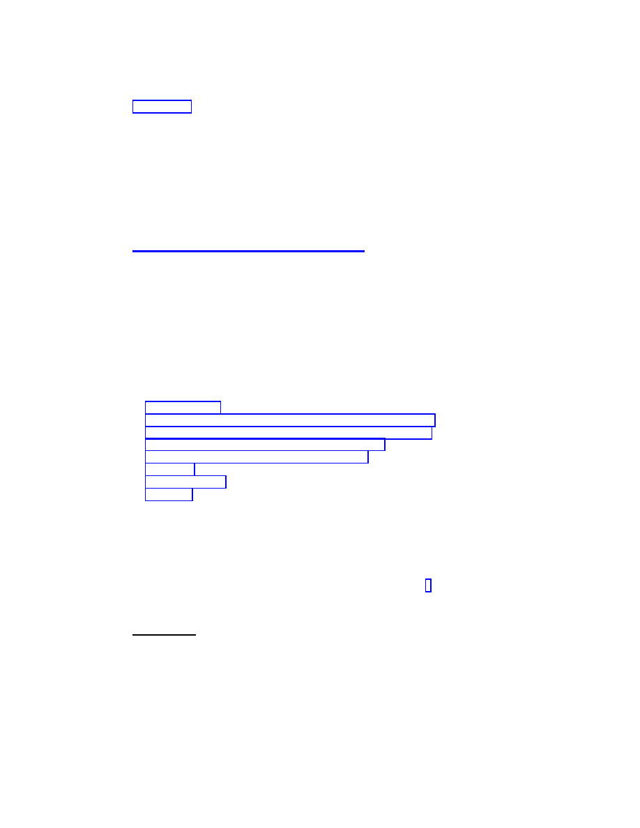
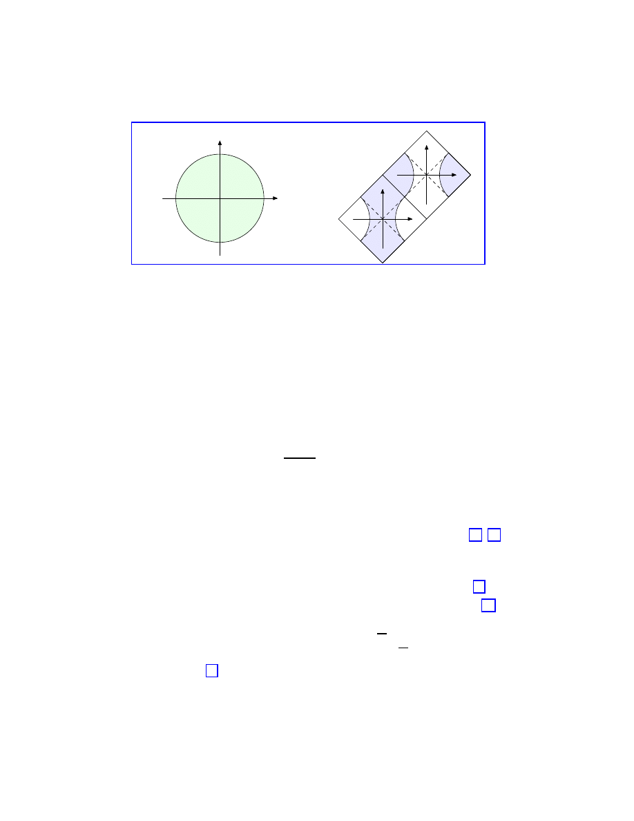
R)/H with the unit disk D, see Figure 1(a), and define mapping
s :
D → SL
2
(
R) and r : G → H as follows
s : a
7→
1
q
1
− |a|
2
1
a
¯
a
1
r :
α
β
¯
β
¯
α
7→
α
|α|
0
0
¯
α
|α|
!
.
(3.4)
6
VLADIMIR V. KISIL
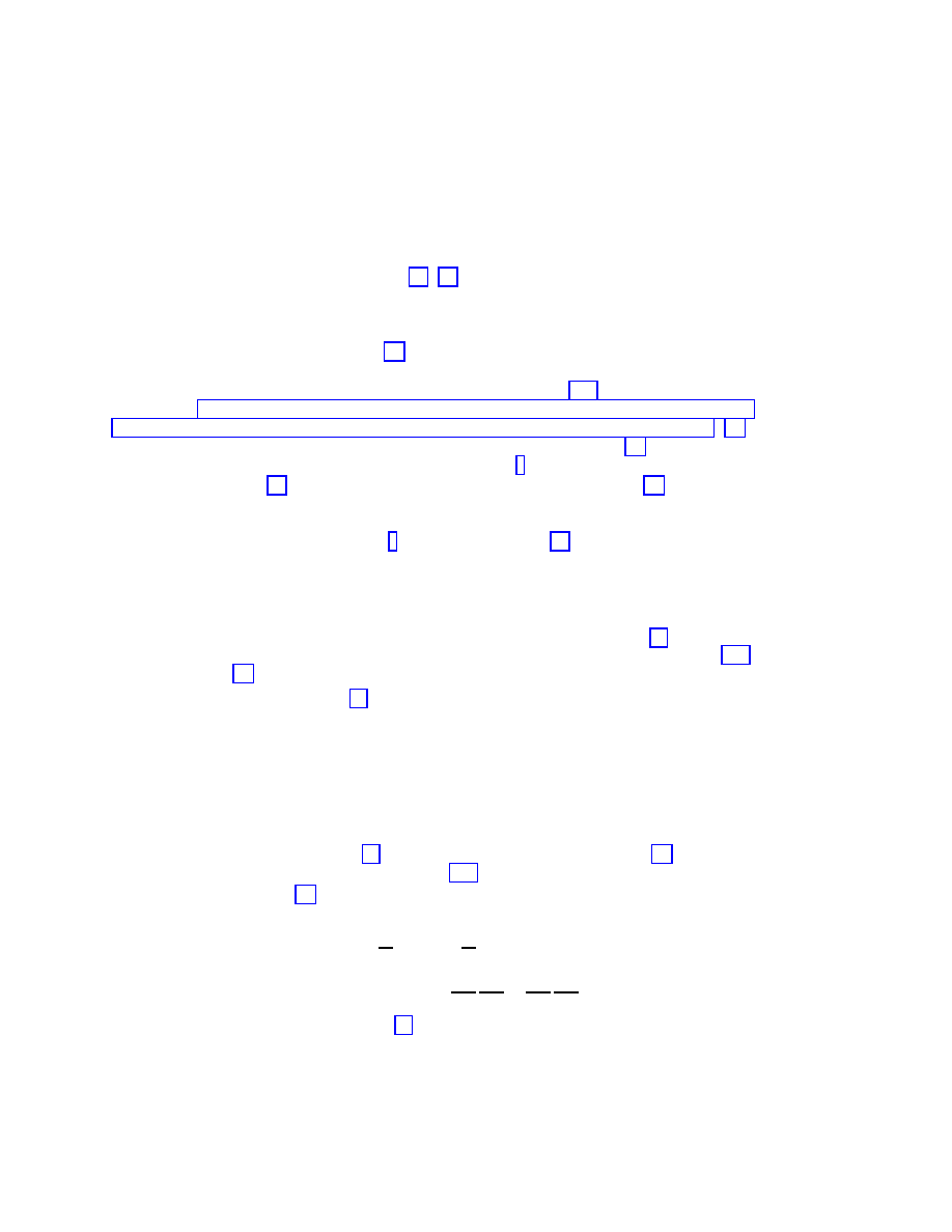
(a)
(b)
C
Figure 1. Two unit disks in elliptic (a) and hyperbolic (b) met-
rics. In (b) squares ACA
0
C
00
and A
0
C
0
A
00
C
00
represent two copies
of
R
2
, their boundaries are the image of the light cone at infinity.
These cones should be glued in a way to merge points with the
same letters (regardless number of dashes). The hyperbolic unit
disk e
D (shaded area) is bounded by four branches of hyperbola.
Dashed lines are light cones at origins.
The formula g : a
7→ g · a = s
−1
(g
−1
∗ s(a)) associates with a matrix g
−1
=
α
β
¯
β
¯
α
the fraction-linear conformal transformation of
D of the form
g : z
7→ g · z =
αz + β
¯
βz + ¯
α
,
g
−1
=
α
β
¯
β
¯
α
,
(3.5)
which also can be extended to a transformation of ˙
C (the one-point compactification
of
C). Here X = D is two dimensional conformal configuration space.
(d) Now we use SL
2
(
R) in the form of a Lorentz type group SO
e
(1, 1). It is
convenient to represent its elements again as 2
× 2-matrices but this time with
Clifford algebra values. This four real dimensional Clifford algebra
generated by 1 and two imaginary units e
1
and e
2
such that
e
2
1
=
−e
2
2
=
−1,
e
1
e
2
=
−e
2
e
1
.
We use Sanserif font for elements of
C`(1, 1). Then SL
2
(
R) is represented [23] by
matrices
a
b
−b a
where a¯
a
− b¯b = 1. We have a decomposition similar to (3.3):
a
b
−b a
=
|a|
1
ba
−1
−ba
−1
1
a
|a|
0
0
a
|a|
!
.
(3.6)
It could be seen [23] that ba
−1
∈ R
1,1
, i.e. is a two-dimensional vector in Minkowski
space. But now we could not get that
ba
−1
< 1, or equivalently we could not
separate:
(1) topologically the Minkowski space
R
1,1
into interior and exterior of the unit
circle;

DESCARTES AND KLEIN ON NONCOMMUTATIVE GEOMETRY
7
(2) analytically L
2
on the unit “circle” into subspaces of analytic and antianalytic
functions;
(3) physically the time axis into the future and the past halves,
because M¨
obius (linear-fractional) transformations mix both sets in each case. A
way out is known and is the same both in physical [39] and mathematical [23]
situations: we need to take a double cover of
R
1,1
and chose the “unit disk” e
D as
shown on Figure 1(b) and explained in its caption.
Matrices of the form
a 0
0
a
=
e
e
1
e
2
τ
0
0
e
e
1
e
2
τ
, a = e
e
1
e
2
τ
= cosh τ +
e
1
e
2
sinh τ,
τ
∈ R comprise a subgroup of hyperbolic rotations in R
1,1
which we
denote by A. We define an embedding s of e
D for our realization of SL
2
(
R) by the
formula:
s : u
7→
1
√
1 + u
2
1
u
−u 1
,
r :
a
b
−b a
7→
a
|a|
0
0
a
|a|
!
(3.7)
The formula g : u
7→ s
−1
(g
· s(u)) gives the linear-fraction transformation e
D → eD
conformal in the hyperbolic metric:
g : u
7→ g · u =
au + b
−bu + a
,
g
−1
=
a
b
−b a
,
(3.8)
which is similar to (3.5). We get two dimensional relativistic space-time. The
appearance of Clifford algebra in relativistic case is expectable [13, 35].
♦
In the following we call X just space understanding that in different realisations
it could be either a configuration space or phase space or space-time.
3.2. The Vacuum and Reduced Wavelet Transform. We are ready to
explain the rˆ
ole of the subgroup H in the coherent states construction: it selects
the vacuum as its eigenvector among all possible physical states. Thereafter having
the chosen vacuum we can generate all possible states of the system from a repre-
sentation ρ of G by isometric operators in a Banach space B. Coherent states are
parametrised by points of the space X = G/H.
Definition 3.2. [25] Let G, H, X = G/H, s : X
→ G, ρ : G → L(B) be as
before. We say that b
0
∈ B is a vacuum vector if for all h ∈ H
ρ(h)b
0
= χ(h)b
0
,
χ(h)
∈ C.
(3.9)
We say that set of vectors b
x
= ρ(x)b
0
, x
∈ X form a family of coherent states if
there exists a continuous non-zero linear functional l
0
∈ B
∗
, called the analysing
functional, such that
(1)
kb
0
k = 1, kl
0
k = 1, hb
0
, l
0
i 6= 0;
(2) ρ(h)
∗
l
0
= ¯
χ(h)l
0
, where ρ(h)
∗
is the adjoint operator to ρ(h);
(3) The following equality holds
Z
X
ρ(x
−1
)b
0
, l
0
hρ(x)b
0
, l
0
i dµ(x) = hb
0
, l
0
i .
(3.10)
With analysing functional we are able to decompose any state as a superposition
of the coherent states.
8
VLADIMIR V. KISIL
Definition 3.3. The reduced wavelet transform
W from a Banach space B
to a space of function F (X) on a homogeneous space X = G/H defined by a
representation ρ of G on B, a vacuum vector b
0
and a test functional l
0
is:
W : v 7→ ˆv(x) = [Wv](x) =
ρ(x
−1
)v, l
0
=
hv, ρ
∗
(x)l
0
i .
(3.11)
The inverse wavelet transform
M from F (X) to B is given by the formula:
M : ˆv(x) 7→ M[ˆv(x)] =
Z
X
ˆ
v(x)b
x
dµ(x) =
Z
X
ˆ
v(x)ρ(x) dµ(x)b
0
.
(3.12)
The geometric action (3.2) of G : X
→ X defines a representation λ(g) :
F (X)
→ F (X) induced by a character χ of H as follows
[λ(g)f](x) = χ(r(g
−1
· x))f(g
−1
· x).
(3.13)
For the case of trivial H =
{e} the representation (3.13) becomes the left regular
representation ρ
l
(g) of G on L
2
(G).
Proposition 3.4. We have:
(1) The reduced wavelet transform
W and the inverse wavelet transform M
intertwine ρ and the representation λ (3.13) on F (X):
Wρ(g) = λ(g)W
and
Mλ(g) = ρ(g)M
forallg
∈ G.
(3.14)
(2) There is an isomorphism property:
hWv, M
∗
l
i
F (X)
=
hv, li
B
,
∀v ∈ B,
l
∈ B
∗
(3.15)
(3) The image F (X) of B under
W is λ-invariant subspace of C (G).
There is a physical meaning of (3.14): having a representation ρ of G in an
abstract space L(B) of observables we could introduce a space X and realise B as
functions on X with a geometric action λ (3.13) instead of an abstract ρ. This
advantage allows us to use the intertwining property (3.14) in new Definition 4.1
of functional calculus and Definition 5.1 of quantisation instead of the traditional
algebraic homomorphism property.
Theorem 3.5. The composition of transforms
M and W
P = MW : B → B
(3.16)
is a projection of B to its linear subspace for which b
0
is cyclic. Particularly if ρ is
an irreducible representation then the inverse wavelet transform
M is a left inverse
operator on B for the wavelet transform
W: MW = I.
Example 3.6. (a) We take a representation σ
h
of
H in L
p
(
R), 1 < p < ∞ by
operators of shift and multiplication [44,
§ 1.1]:
σ
h
(s, z) : f(y)
→ [σ
h
(s, z)f](y) = e
i(2sh
−
√
2hvy+huv)
f(y
−
√
2hu),
z = u + iv,
(3.17)
It is the Schr¨
odinger representation with parameter h. As a character of H =
R
2
we take the χ(s, u) = e
2it
. The corresponding test functional l
0
satisfying to 3.2(2)
is the integration l
0
(f) = (2π)
−n/2
R
R
n
f(y) dy. Thus the wavelet transform (3.11)
is
ˆ
f (x) =
Z
R
n
σ(s(x)
−1
)f(y) dy = (2π)
−n/2
Z
R
n
e
i
√
2xy
f(y) dy
(3.18)
DESCARTES AND KLEIN ON NONCOMMUTATIVE GEOMETRY
9
and is nothing else but the Fourier transform. There is no a vacuum vector in our
space B, see physical implications of an absence of vacuum in [40]. We however
could proceed as in [25,
§ 2.3] and take a bigger space B
0
= L
∞
(
R
n
)
⊃ B with
the vacuum vector b
0
(y)
≡ (2π)
−n/2
∈ B
0
. Then coherent states are b
x
(y) =
(2π)
−n/2
e
−i
√
2xy
and the inverse wavelet transform (3.12) is defined by the inverse
Fourier transform
f(y) =
Z
R
n
ˆ
f(y)b
x
(y) dx = (2π)
−n/2
Z
R
n
ˆ
f(y)e
−i
√
2xy
dx.
W and M intertwine the left regular representation — multiplication by e
i
√
2yv
with
operators
[λ(g)f](x)
=
χ(r(g
−1
· x))f(g
−1
· x) = e
i
√
2
·0
f(x
−
√
2u) = f(x
−
√
2u),
i.e. with Euclidean shifts. From (3.15) follows the Plancherel identity:
Z
R
n
ˆ
v(y)ˆ
l(y) dy
=
Z
R
n
v(x)l(x) dx.
Thus our construction generate all important properties of the Fourier transform.
The Schr¨
odinger representation is irreducible on
S(R
n
) thus
M = W
−1
. There-
after the operator (3.16) representing operators
MW = WM = 1 correspondingly
give an integral resolution of the Dirac delta δ(x):
[]δ(x
− y) = (2π)
−n/2
Z
R
n
e
iξ(x
−y)
dξ.
(b) As a subgroup H we select now the center of
H consisting of elements (s, 0). As
a “vacuum vector” we will select the original vacuum vector of quantum mechanics—
the Gauss function f
0
(x) = e
−x
2
/2
which belongs to all L
p
(
R
n
). Its transformations
are as follow:
f
g
(x) = [ρ
(s,z)
f
0
](x) =
e
2it
−z¯
z/2
e
−(¯
z
2
+x
2
)/2+
√
2¯
zx
.
Particularly [ρ
(s,0)
f
0
](x) = e
−2it
f
0
(x), i.e., it really is a vacuum vector in the sense
of our Definition 3.2 with respect to H. For the same reasons we could take l
0
(x) =
e
−x
2
/2
∈ L
q
(
R
n
), p
−1
+ q
−1
= 1 as the analysing functional.
Coherent states f
g
(x) = [ρ
(0,z)
f
0
](x) belongs to L
q
(
R
n
)
⊗ L
p
(
C
n
) for all p > 1
and q > 1, p
−1
+ q
−1
= 1. Thus transformation (3.11) with the kernel [ρ
(0,z)
f
0
](x)
is an embedding L
p
(
R
n
)
→ L
p
(
C
n
) and is given by the formula
ˆ
f (z)
=
e
−z¯
z/2
π
−n/4
Z
R
n
f(x) e
−(z
2
+x
2
)/2+
√
2zx
dx.
(3.19)
Then ˆ
f (g) belongs to L
p
(
C
n
, dg) or its preferably to say that function ˘
f (z) =
e
z ¯
z/2
ˆ
f (t
0
, z) belongs to space L
p
(
C
n
, e
−|z|
2
dg) because ˘
f (z) is analytic in z. Such
functions for p = 2 form the Segal-Bargmann space F
2
(
C
n
, e
−|z|
2
dg) of functions [6,
38], which are analytic by z and square-integrable with respect the Gaussian mea-
sure e
−|z|
2
dz.
The integral in (3.19) is the well-known Segal-Bargmann transform [6, 38].
The inverse is given by a realization of (3.12):
f(x) =
Z
C
n
˘
f(z)e
−(¯
z
2
+x
2
)/2+
√
2¯
zx
e
−|z|
2
dz.
(3.20)
10
VLADIMIR V. KISIL
The corresponding operator
P (3.16) is an identity operator L
p
(
R
n
)
→ L
p
(
R
n
)
and (3.16) gives another integral presentation of the Dirac delta.
Integral transformations (3.19) and (3.20) intertwines the Schr¨
odinger repre-
sentation (3.17) with the following realization of representation (3.13):
λ(s, z)f(w)
=
ˆ
f
0
(z
−1
· w)¯
χ(t + r(z
−1
· w)) = ˆ
f
0
(w
− z)e
it+i
=(¯
zw)
(3.21)
Meanwhile the orthoprojection L
2
(
C
n
, e
−|z|
2
dg)
→ F
2
(
C
n
, e
−|z|
2
dg) is of a sep-
arate interest and is a principal ingredient in Berezin quantization [7, 9]. Its integral
kernel is
K(z, w)
=
exp
1
2
(
− |z|
2
− |w|
2
) + w ¯
z
.
(c) We continue with the case of G = SL
2
(
R) and H = K. The compact group
K
∼ T has a discrete set of characters χ
m
(h
φ
) = e
−imφ
, m
∈ Z. We consider here
only χ
1
, see [23] for others. Let us take X =
T—the unit circle equipped with the
standard Lebesgue measure dφ normalised in such a way that
Z
T
|f
0
(φ)
|
2
dφ = 1withf
0
(φ)
≡ 1.
(3.22)
From (3.4) one can find that
r(g
−1
∗ s(e
iφ
)) =
¯
βe
iφ
+ ¯
α
¯
βe
iφ
+ ¯
α
,
g
−1
=
α β
¯
β
¯
α
.
Then the action of G on
T defined by (3.5), the equality d(g · φ)/dφ =
¯
βe
iφ
+ ¯
α
−2
and the character χ
1
give the following realization of the formula (3.13):
[ρ
1
(g)f](e
iφ
) =
1
¯
βe
iφ
+ ¯
α
f
αe
iφ
+ β
¯
βe
iφ
+ ¯
α
.
(3.23)
This is a unitary representation—the mock discrete series of SL
2
(
R) [44, § 8.4]. It
is easily seen that K acts in a trivial way (3.9) by multiplication by χ(e
iφ
). The
function f
0
(e
iφ
)
≡ 1 mentioned in (3.22) transforms [ρ
1
(g)f
0
](e
iφ
) = ( ¯
βe
iφ
+ ¯
α)
−1
and in particular has an obvious property [ρ
1
(h
ψ
)f
0
](φ) = e
iψ
f
0
(φ), i.e. it is a
vacuum vector with respect to the subgroup H. The smallest linear subspace
F
2
(X)
∈ L
2
(X) spanned by all these transformations consists of boundary values
of analytic functions in the unit disk and is the Hardy space. Now the reduced
wavelet transform (3.11) takes the form [23]:
ˆ
f (a) = [
Wf](a) =
q
1
− |a|
2
i
Z
T
f(z)
a + z
dz,
(3.24)
where z = e
iφ
. Of course (3.24) is the Cauchy integral formula up to factor
2ρ
q
1
− |a|
2
. The inverse wavelet transform
M gives an integral expression for
orthoprojection Szeg¨
o onto the Hardy space.
(d) Now we consider the same group G = SL
2
(
R) but pick up another subgroup
H = A. Let e
12
denote e
1
e
2
. The mapping from the subgroup A
∼ R to even
Clifford numbers χ
σ
: a
7→ a
e
12
σ
= (exp(e
1
e
2
σ ln a)) = (ap
1
+a
−1
p
2
)
σ
parametrised
by σ
∈ R is a character (in a somewhat generalised sense). It represents an isometric
DESCARTES AND KLEIN ON NONCOMMUTATIVE GEOMETRY
11
rotation of e
T by the angle a. Under the present conditions we have from (3.7):
r(g
−1
∗ s(u)) =
−bu+a
|−bu+a|
0
0
−bu+a
|−bu+a|
!
,
g
−1
=
a
b
−b a
.
Furthermore we can construct a realization of (3.13) on the functions defined
on e
T by the formula:
[ρ
σ
(g)f](v) =
(
−vb + ¯a)
σ
(
−bv + a)
1+σ
f
av + b
−bv + a
,
g
−1
=
a
b
−b a
.
(3.25)
It is induced by the character χ
σ
due to formula
−bv+a = (cx+d)p
1
+(bx
−1
+a)p
2
,
where x = e
t
and it is a cousin of the principal series representation (see [30,
§ VI.6,
Theorem 8], [44,
§ 8.2, Theorem 2.2]). The subspaces of vector valued and even
number valued functions are invariant under (3.25) and the representation is unitary
with respect to the following inner product:
hf
1
, f
2
i
e
T
=
Z
e
T
¯
f
2
(t)f
1
(t) dt.
We select function f
0
(u)
≡ 1 as our vacuum vector, it is a singular one in the
same sense as e
ixξ
is singular for the Fourier transform in Example 3.6(a). Its
transformations
f
g
(v) = [ρ
σ
(g)f
0
](v) =
1 + u
2
1/2
(
−vb + ¯a)
σ
(
−bv + a)
1+σ
(3.26)
and in particular the identity [ρ
σ
(g)f
0
](v) = ¯
a
σ
a
−1−σ
f
0
(v) = a
−1−2σ
f
0
(v) for g
−1
=
a
0
0
a
demonstrates that it is a vacuum vector. Thus we define the reduced
wavelet transform accordingly to (3.7) and (3.11) by the formula:
[
W
σ
f](u)
=
1 + u
2
1/2
e
12
Z
eT
(
−ue
1
z + 1)
σ
z
σ
(
−e
1
u + z)
1+σ
dz f(z)
(3.27)
where z = e
e
12
t
is the new monogenic variable and dz = e
12
e
e
12
t
dt—its differential.
The integral (3.27) is a singular one, its four singular points are intersections of the
light cone with the origin in u with the unit circle e
T.
The explicit similarity between (3.24) and (3.27) allows us to consider transfor-
mation
W
σ
(3.27) as an analog of the Cauchy integral formula and the linear space
H
σ
(e
T) generated by the coherent states f
u
(z) (3.26) as the correspondence of the
Hardy space H
2
(
T).
♦
3.3. The Dirac (Cauchy-Riemann) and Laplace Operators. Consider-
ation of Lie groups is hardly possible without consideration of their Lie algebras,
which are naturally represented by left and right invariant vectors fields on groups.
On a homogeneous space X = G/H we have also defined a left action of G and
can be interested in left invariant vector fields (first order differential operators).
Due to the irreducibility of F
2
(x) under left action of G every such vector field
D restricted to F
2
(x) is a scalar multiplier of identity D
|
F
2
(x)
= cI. We are in
particular interested in the case c = 0.
Definition 3.7. [5, 29] A G-invariant first order differential operator
D
ρ
: C
∞
(X,
S ⊗ V
ρ
)
→ C
∞
(X,
S ⊗ V
ρ
)
12
VLADIMIR V. KISIL
such that
W(F
2
(X))
⊂ ker D
ρ
is called (Cauchy-Riemann-)Dirac operator on X =
G/H associated with an irreducible representation ρ of H in a space V
ρ
and a spinor
bundle
S.
The Dirac operator is explicitly defined by the formula [29, (3.1)]:
D
ρ
=
n
X
j=1
ρ(Y
j
)
⊗ c(Y
j
)
⊗ 1,
(3.28)
where Y
j
is an orthonormal basis of p = h
⊥
—the orthogonal completion of the Lie
algebra h of the subgroup H in the Lie algebra g of G; ρ(Y
j
) is the infinitesimal
generator of the right action of G on X; c(Y
j
) is Clifford multiplication by Y
i
∈ p
on the Clifford module
S. We also define an invariant Laplacian by the formula
∆
ρ
=
n
X
j=1
ρ(Y
j
)
2
⊗
j
⊗ 1,
(3.29)
where
j
= c(Y
j
)
2
is +1 or
−1. Note that the Dirac operator (3.28) is not a factor
of the Laplacian (3.29) unless all commutators [Y
i
, Y
j
] vanish. Thus null-solutions
of D
ρ
is not necessarily the null-solutions of ∆
ρ
a priory. But this happens under
our assumptions.
Proposition 3.8. [23] Let all commutators of vectors of h
⊥
belong to h, i.e.
[h
⊥
, h
⊥
]
⊂ h. Let also f
0
be an eigenfunction for all vectors of h with eigenvalue 0
and let also
Wf
0
be a null solution to the Dirac operator D. Then ∆f(x) = 0 for
all f(x)
∈ F
2
(X).
Example 3.9. (a) With G =
H, H = R
2
, and X =
R the L
2
(X) is irreducible
therefore both the Dirac and Laplace operators are identically zero.
(b) With G =
H, H = R, and X = R
2
we could take just
C as a “Clifford algebra”
sufficient in that case. The orthogonal completion to the centre (s, 0, 0) generates
two dimensional Euclidean shifts on
R
2
=
C, cf. Example 3.1(b). As an orthogonal
basis in that subspace we could take the differential operators ∂/∂x
1
and ∂/∂x
2
,
then we got the following realisation of (3.28) and (3.29):
D =
∂
∂x
1
− i
∂
∂x
2
and
∆ =
∂
2
∂x
2
1
+
∂
2
∂x
2
2
,
i.e. the classic Cauchy-Riemann and Laplace operators. This is a particular case
of invariant operators on nilpotent Lie groups considered in [12] and the inclusion
[h
⊥
, h
⊥
]
⊂ h needed in Proposition 3.8 follows from the nilpotency of H.
(c) Let G = SL
2
(
R) and H be its one-dimensional compact subgroup K. Then h
⊥
is spanned by two vectors Y
1
= A and Y
2
= B. In such a situation we can again use
C instead of the Clifford algebra C`(0, 2). Then formula (3.28) takes a simple form
D = ρ(A + iB). Infinitesimal action of this operator in the upper-half plane follows
from calculation in [30, VI.5(8), IX.5(3)], it is [D
H
f](z) =
−2iy
∂f(z)
∂ ¯
z
, z = x + iy.
Making the Cayley transform we can find its action in the unit disk D
D
: again the
Cauchy-Riemann operator
∂
∂ ¯
z
is its principal component. An explicit calculation of
D
H
was done in [23] and gives the expected answer
D
H
= iρ(A) + ρ(B) = 2yi∂
2
+ 2y∂
1
= 2y
∂
∂ ¯
z
,
DESCARTES AND KLEIN ON NONCOMMUTATIVE GEOMETRY
13
which is just a conformal invariant variant of the Cauchy-Riemann equation. The
corresponding operator ∆ is an invariant Laplacian.
(d) In
R
1,1
the subgroup H = A and its orthogonal completion is spanned by B
and Z. Thus the associated Dirac operator has the form D = e
1
ρ(B) + e
2
ρ(Z).
We need infinitesimal generators of the right action ρ on the “left” half plane e
H.
Following to [23] we find that:
D
e
H
= e
1
ρ(Z) + e
2
ρ(A) = 2y(e
1
∂
1
+ e
2
∂
2
).
In this case the Dirac operator is not elliptic and as a consequence we have in
particular a singular Cauchy integral formula (3.27). Another manifestation of the
same property is that primitives in the “Taylor expansion” do not belong to F
2
(e
T)
itself, see Example 3.12(d). It is known that solutions of a hyperbolic system (unlike
the elliptic one) essentially depend on the behaviour of the boundary value data.
Thus function theory in
R
1,1
is not defined only by the hyperbolic Dirac equation
alone but also by an appropriate boundary condition. The operator (3.29) in this
case is the wave equation ∆ = y
2
(∂
2
1
− ∂
2
2
).
♦
3.4. The Taylor Expansion. Both the wavelet transform and its inverse are
based on the family of coherent states f
a
. For any decomposition
f
a
(x) =
X
α
ψ
α
(x)V
α
(a)
(3.30)
of the coherent states f
a
(x) by means of functions V
α
(a) (where the sum can become
eventually an integral) we have the Taylor expansion
ˆ
f (a)
=
Z
X
f(x) ¯
f
a
(x) dx =
Z
X
f(x)
X
α
¯
ψ
α
(x) ¯
V
α
(a) dx
=
X
α
Z
X
f(x) ¯
ψ
α
(x) dx ¯
V
α
(a) =
∞
X
α
¯
V
α
(a)f
α
,
(3.31)
where f
α
=
R
X
f(x) ¯
ψ
α
(x) dx. However to be useful within the presented scheme
such a decomposition should be connected with the structures of G, H, and the
representation ρ. We will use a decomposition of f
a
(x) by the eigenfunctions V
α
of
the operators ρ(h), h
∈ h.
Definition 3.10. Let F
2
(X) =
R
A
H
α
dα be a spectral decomposition with
respect to the operators ρ(h), h
∈ h. Then the decomposition
f
a
(x) =
Z
A
V
α
(a)f
α
(x) dα,
(3.32)
where f
α
(x)
∈ H
α
and V
α
(a) : H
α
→ H
α
is called the Taylor decomposition of the
Cauchy kernel f
a
(x).
Note that the Dirac operator D is defined in the terms of left invariant vector
fields and therefore commutes with all ρ(h). Thus it also has a spectral decompo-
sition over spectral subspaces of ρ(h):
D =
Z
A
D
δ
dδ.
(3.33)
Proposition 3.11. [23] The following two equivalent statements links together
the Dirac operator and the Taylor decomposition in mathematical and physical lan-
guages respectively.
14
VLADIMIR V. KISIL
(1) If spectral measures dα and dδ from (3.32) and (3.33) have disjoint supports
then the image of the Cauchy integral belongs to the kernel of the Dirac
operator.
(2) We say that V
a
is negative if DV
a
6= 0 and V
a
is positive ψ
a
6= 0 in the
decomposition (3.30). If the intersection of positive and negative states is
void then the physical states from F (X) are null solutions of the Dirac
operator.
Example 3.12. (a) For G =
H and H = R
2
the only eigenvectors of H in the
Schr¨
odinger representation (3.17) are exponents e
ixξ
and the “Taylor decomposi-
tion” over them is in fact the Fourier integral. Note that singularity of the vacuum,
like in the case (d) below, implies that the primitive monomials are also outside
our space
F(X). Here the support of dα is R and from Example 3.9(a) the support
of dδ is the empty set, i.e they are disjoint.
(b) For G =
H and H = R the subgroup H acts trivially as multiplication by a
scalar on any function thus leave us an excessive freedom in th choice of the Taylor
decomposition. We may wish to use Proposition 3.11 as a guideline. Example 3.9(b)
tells that the Dirac operator is the Cauchy-Riemann operator ∂/∂ ¯
z. Thus to get a
decomposition over a disjoint support we may chose the monomial z
k
for the Taylor
decomposition. The same choice is dictated if we wish to obtained the minimum
uncertainty states [34].
(c) Let G = SL
2
(
R) and H = K be its maximal compact subgroup and ρ
1
be
described by (3.23). H acts on
T by rotations. It is one dimensional and eigen-
functions of its generator Z are parametrised by odd integers (due to compactness
of K). Moreover, on the irreducible Hardy space these are positive odd integers
n = 1, 3, 5 . . . and corresponding eigenfunctions are f
2n+1
(φ) = e
inφ
. Negative
integers span the space of anti-holomorphic function and the splitting reflects the
existence of analytic structure given by the Cauchy-Riemann equation from Exam-
ple 3.9(c). The decomposition of coherent states f
a
(φ) by means of this functions
is well known:
f
a
(φ) =
q
1
− |a|
2
¯
ae
iφ
− 1
=
∞
X
n=1
q
1
− |a|
2
¯
a
n
−1
e
i(n
−1)φ
=
∞
X
n=1
V
n
(a)f
n
(φ),
where V
n
(a) =
q
1
− |a|
2
¯
a
n
−1
. This is the classical Taylor expansion up to multi-
pliers coming from the invariant measure.
(d) Let G = SL
2
(
R), H = A, and ρ
σ
be described by (3.25). Subgroup H acts on
e
T by hyperbolic rotations:
ρ : z = e
1
e
e
12
t
→ e
2e
12
τ
z = e
1
e
e
12
(2τ+t)
,
t, τ
∈ e
T.
Then for every p
∈ R the function f
p
(z) = (z)
p
= e
e
12
pt
where z = e
e
12
t
is an
eigenfunction in the representation (3.25) for a generator a of the subgroup H = A
with the eigenvalue 2(p
− σ) − 1, cf. with (a) above. Again, due to the analytical
structure reflected in the Dirac operator, we only need negative values of p to
decompose the Cauchy integral kernel. Thereafter for a function f(z)
∈ F
2
(e
T) we
have the following Taylor expansion of its wavelet transform [23]:
[
W
0
f](u) =
Z
∞
0
(e
1
u)
[p]
− 1
e
1
u
− 1
f
p
dp,
where
f
p
=
Z
eT
tz
−p
dzf(z).
(3.34)

DE
S
C
A
R
T
E
S
A
N
D
K
L
E
IN
O
N
N
O
N
C
O
M
M
U
T
A
T
IV
E
G
E
O
M
E
T
R
Y
1
5
Notion
G =
H, H = R
2
G =
H, H = R
2
G = SL
2
(
R), H = K G = SL
2
(
R), H = A · · ·
Space X
Real line
R
Complex line
C
Unit disk
D
Disk on Fig. 1(b)
· · ·
Physical meaning
Configuration space
Phase space
Conformal 2d space
Space-time (2d)
· · ·
Functional space B
L
p
(
R)
L
p
(
C)
L
p
(
T)
L
p
(e
T)
· · ·
Representation
Schr¨
odinger
Schr¨
odinger
Conformal maps
Conformal maps
· · ·
Vacuum vector
f
0
(x)
≡ 1
f
0
(x) = e
−x
2
/2
f
0
(t)
≡ 1
f
0
(t)
≡ 1
· · ·
Wavelet transform
W
Fourier transform
Segal-Bargmann (SB) tr.
Cauchy integral
Formula (3.27)
· · ·
Inverse transform
M
Fourier transform
Inverse SB transform
Szeg¨
o projection
· · ·
Image F (X)
Whole L
2
(
R)
Segal-Bargmann space
Hardy space
Monogenic space
· · ·
Dirac operator
Null operator
Cauchy-Riemann oper.
Cauchy-Riemann op.
Dirac operator
· · ·
Laplace operator
Null operator
Laplace operator
Laplace operator
Wave operator
· · ·
Taylor expansion
Fourier integral
Taylor expansion
Taylor expansion
Formula (3.34)
· · ·
Image of convolution [25]
Weyl PDO (4.1) [16, 43]
Wick operator [7, 16]
T¨
oplitz operator
Sing.Int.Op. [43]
· · ·
Table 1. Periodic table of elements of analytic function theory. The dots at the end symbolise an absence of the table end.
16
VLADIMIR V. KISIL
The last integral is similar to the Mellin transform [30,
§ III.3], [44, Chap. 8, (3.12)],
which naturally arises from the principal series representations of SL
2
(
R).
♦
Our presentation fits into Table 1, which is an extended version of the table
from paper [24]. It was called there the “periodic table” of function theory and it
was guessed that it could help to discover new analytic function theories just like the
periodic table of chemical elements by D. Mendeleev help to find new elements. The
chain (d) of above examples was presented in [23] as a sample of such a theory. Not
all theretically possible function theory are reasonable just like not all theoretical
combination of protons and neutrons gives a stable chemical atom. However there
are still some more interesting function theories to descover.
We interrupt here with our overview of the coherent state construction, but
much more could be derived from it. See books [1, 34] for more examples of groups
and physical aspects of the theory. Paper [25] contains further connections with
operator theory, symbolic calculus, PDO, and Toeplitz operators which we did not
mention here at all, see the last raw of the Table 1 however.
4. Functional Calculus as an Intertwining Operator
Each problem that I solved became a rule which served
afterwards to solve other problems.
Descartes Discours de la M´
ethode, 1637
We saw in the preceeding section that coherent states naturally generate many
principal objects of analysis and function theory. Particularly the wavelet transform
as an intertwining operator links different spaces with the same symmetry. Could
we export this observation to other areas? There are many cases where function
spaces provide a model for more complicated objects, i.e. a functional calculus of
operators and quantisation procedure. Thus they are the first candidates for an
application of that technique.
There are several types of functional calculi, e.g. for selfadjoint bounded [36,
§ VII.2] or unbounded [36, § VIII.3] operators, normal operators [15, § VII.3],
several commuting selfadjoint operators [42]. All of them are defined as algebraic
homomorphisms from an algebra of function to an algebra of operators with some
additional properties. On the language of identification (2.1) this means that func-
tional and operator spaces are forced to have the same system of coordinates. The
only exception from that rule is the Weyl functional calculus [2] which is defined
just by an integral formula and is not traditionally obliged to preserve any algebraic
structure. That calculus is a generalisation of the Weyl quantisation [16,
§ 2.1]
a
h
(p, q)
7→ a
h
(D, X) =
Z Z
ˆ
a(x, y)σ
h
(0, x, y) dx dy
(4.1)
obtained by an integration of the Schr¨
odinger representation σ
h
(3.17).
However there is no need to be so restricted in our choice: we could give a
meaningful general definition [22] of functional calculus without any references to
an algebraic homomorphism property at all. Moreover we can define a functional
calculus not only for an operator algebra A but also for any A-module M [28]. Let
there be two continuous representations ρ
f
and ρ
a
of the same topological group
G such that ρ
f
act on function space F (X,
C) with a vacuum vector b
0
∈ F (X, C)
and action of ρ
a
on an M -valued function space F (X, M ) in a way determined by
an element a
∈ A.
DESCARTES AND KLEIN ON NONCOMMUTATIVE GEOMETRY
17
Definition 4.1. An analytic functional calculus of an element a
∈ A is a
continuous linear map Φ : F (X,
C) → F (X, M) : f(w) 7→ [Φf] if the following
conditions fulfil
(1) Φ is an intertwining operator between ρ
f
and ρ
a
, namely
[Φρ
1
(g)f] = ρ
a
(g)[Φf],
(4.2)
for all g
∈ G and f ∈ F (A, C).
(2) Φ maps the vacuum vector b
0
for the representation ρ
f
to the vacuum
vector b
a
∈ F (X, M) for the representation ρ
a
:
[Φb
0
] = b
a
.
(4.3)
We will illustrate advantages of this approach by a construction of functional
calculus for a finite dimensional non-normal matrix. We use to this end the group
SL
2
(
R) together with its discrete series mock representation ρ
1
(3.23) in L
2
(
T)
as a model [28] for a corresponding representation related to a matrix. Let A be
the algebra of complex valued n
× n matrix, e be its unit and a ∈ A have all its
eigenvalues in the unit circle
D. Then we could define linear-fraction transformation
g
· a of a by the formula:
g
−1
a = (¯
αa
− ¯
βe)(αe
− βa)
−1
,
where
g
−1
=
¯
α
− ¯
β
−β
α
,
(4.4)
in analogy with the point transformation (3.5). The set all matrices (4.4) for g
∈
SL
2
(
R) becomes a SL
2
(
R)-homogeneous space. Similarly the resolvent R(g
−1
a) =
(¯
αe
− ¯
βa)
−1
is well defined for all g
∈ SL
2
(
R). Let M = C
n
be a natural left
A
-module and let us consider a space of M -valued functions on
D. Analogously
to (3.23) we define a representation ρ
a
of SL
2
(
R) as follows:
(ρ
a
(g)f)(z) = R(g
−1
a)f
¯
αz
− ¯
β
αe
− βz
,
where
g
−1
=
¯
α
− ¯
β
−β
α
.
(4.5)
Let b
0
(z)
≡ 1 be the vacuum vector of ρ
1
and let H
2
(
D, M) the minimal ρ
a
-
invariant space of M -valued functions containing all functions b
x
(z) = x
⊗ b
0
(z),
x
∈ M. Then the functional calculus in the sense of Definition 4.1 from H
2
(
D)
to H
2
(
D, M) could be constructed [25, Prop. 2.16] with the help of intertwining
properties from Proposition 3.4. Indeed if we define Φ =
M
ρ
a
W
ρ
1
then:
Φρ
1
(g) =
M
ρ
a
W
ρ
1
ρ
1
(g) =
M
ρ
a
λ(g)
W
ρ
1
= ρ
a
(g)
M
ρ
a
W
ρ
1
= ρ
a
(g)Φ.
The explicit integral formula for Φ coincides with the integral formula of Dunford-
Riesz analytic functional calculus [15, Thm. VII.1.10]:
[][Φf](x, z) =
Z
T
f(t)(za
− te)
−1
dtx.
Now we can use the constructed functional calculus to get a better spectral
characterisation of a than just the set of its eigenvalues. The definition used in [2]
to define the Weyl spectrum of operator is suitable for the generalisation.
Definition 4.2. [28] A spectrum of an operator a is the support of a functional
calculus Φ : f(x)
7→ f(a).
Because now the functional calculus is an intertwining operator its support
is a collection of indecomposable intertwining operators between ρ
1
and ρ
a
. The
entire space H
2
(
D, M) splits into ρ
a
-invariant subspaces V
λ,k
generated by functions
18
VLADIMIR V. KISIL
b
x
(z) = x
⊗b
x
(z), where x is a kth root vector for an eigenvalue λ, i.e. (a
−λe)
k
x = 0
and (a
−λe)
k
−1
x
6= 0. Such a minimal ρ
a
-invariant subspace V
λ,k
up to similarity is
described by the corresponding pair (λ, k), λ
∈ D, k ∈ N. To get their classification
we need the following notion.
Definition 4.3. [33, Chap. 4] Two holomorphic functions have nth order con-
tact in a point if their value and their first n derivatives agree at that point, in other
words their Taylor expansions are the same in first n + 1 terms.
A point (z, u
(n)
) = (z, u, u
1
, . . . , u
n
) of the jet space
J
n
∼ D × C
n
is the
equivalence class of holomorphic functions having nth contact at the point z with
the polynomial:
p
n
(w) = u
n
(w
− z)
n
n!
+
· · · + u
1
(w
− z)
1!
+ u.
(4.6)
For a fixed n each holomorphic function f :
D → C has nth prolongation (or
n-jet ) j
n
f :
D → C
n+1
:
j
n
f(z) = (f(z), f
0
(z), . . . , f
(n)
(z)).
(4.7)
The graph Γ
(n)
f
of j
n
f is a submanifold of
J
n
which is section of the jet bundle over
D with a fibre C
n+1
. We also introduce a notation J
n
for the map J
n
: f
7→ Γ
(n)
f
of a holomorphic f to the graph Γ
(n)
f
of its n-jet j
n
f(z) (4.7).
One can prolong any map of function ψ : f(z)
7→ [ψf](z) to a map ψ
(n)
of
n-jets by the formula
ψ
(n)
(J
n
f) = J
n
(ψf).
(4.8)
For example such a prolongation ρ
(n)
1
of the representation ρ
1
of the group SL
2
(
R)
in H
2
(
D) (as any other representation of a Lie group [33]) will be again a repre-
sentation of SL
2
(
R). Equivalently we could say that J
n
intertwines ρ
1
and ρ
(n)
1
:
J
n
ρ
1
(g) = ρ
(n)
1
(g)J
n
.
Of course, the representation ρ
(n)
1
is not irreducible: any jet subspace
J
k
, 0
≤ k ≤ n
is ρ
(n)
1
-invariant subspace of
J
n
.
Coming back to our representation ρ
a
(4.5) we could characterise its minimal
component as follows.
Proposition 4.4. [28] Restriction of ρ
a
to V
λ,k
is equivalent to the extension
ρ
(k)
1
of ρ
1
in the kth jet space
J
k
. Consequently the spectrum of a (defined via the
functional calculus Φ) consists of exactly n pairs (λ
i
, k
i
), λ
i
∈ D, k
i
∈ N, 1 ≤ i ≤ n
some of whom could coincide.
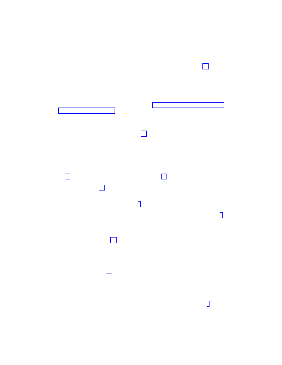
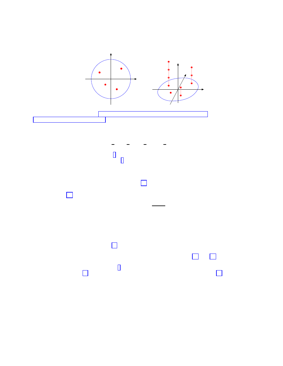
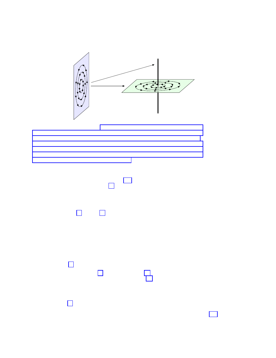
Example 4.5. Let J
k
(λ) denote the Jordan block of the length k for the eigen-
value λ. On the Fig. 2 there are two pictures of the spectrum for the matrix
a = J
3
3
4
e
iπ/4
⊕ J
4
2
3
e
i5π/6
⊕ J
1
2
5
e
−i3π/4
⊕ J
2
3
5
e
−iπ/3
.
Part (a) represents the conventional two-dimensional image of the spectrum, i.e.
eigenvalues of a, and (b) describes spectrum spa arising from the wavelet construc-
tion. The first image did not allow to distinguish a from many other essentially
DESCARTES AND KLEIN ON NONCOMMUTATIVE GEOMETRY
19
(a)
X
Y
(b)
X
Y
Z
Figure 2. Is spectrum flat (a) or three dimensional (b)—depends
from viewpoint.
different matrices, e.g. the diagonal matrix
diag
3
4
e
iπ/4
,
2
3
e
i5π/6
,
2
5
e
−i3π/4
,
3
5
e
−iπ/3
.
At the same time the Fig. 2(b) completely characterise a up to a similarity. Note
that each point of spa on Fig. 2(b) corresponds to a particular root vector.
The three dimensional spectrum of matrices obeys the spectral mapping theo-
rem which is a refined version of the classic theorem about mapping of eigenvalues.
Theorem 4.6 (Spectral mapping). [28] Let φ :
D → D be a holomorphic map,
let us define [φ
∗
f](z) = f(φ(z)) and its prolongation φ
(n)
∗
onto the jet space
J
n
by (4.8). Its associated action on the pairs (λ, k) is given by the formula:
φ
(n)
∗
(λ, k) =
φ(λ),
k
deg
λ
φ
,
where deg
λ
φ denotes the degree of zero of the function φ(z)
− φ(λ) at the point
z = λ and [x] denotes the integer part of x. Then
spφ(a) = φ
(n)
∗
spa.
The explicit expression for φ
(n)
∗
which involves derivatives of φ upto nth order
is known, see for example [17, Thm. 6.2.25], but was not understood before as form
of spectral mapping.
To finish with this topic we will note that our Definitions 4.1 and 4.2 are
not restricted to the case SL
2
(
R) only. They are suitable for any group G and
subgroup H from the Table 1. For example, Segal-Bargmann type calculus was
outlined in [25] and monogenic calculus of several noncommuting operators in [22].
This directions of research still waits a careful exploration.
5. Quantisation from the Symplectic Invariance
Approach your problem from the right end and begin with
the answer. Then one day, perhaps you will find the final
question.
R. van Gulik The Hermit Clad in Crane Feather
It is well known that quantum mechanics is full of paradoxes. The more gen-
eral is the following: there are a lot working tools and tricks which give numerical
20
VLADIMIR V. KISIL
predictions for almost all observable effects, but the majority of them are mathe-
matically unsound and philosophically obscure. The basic example is the question
of quantisation itself.
It is oftenly said that quantum mechanics is superior to the classical one but
unfortunately we are not able to percept its glory directly. To obtain a quantum
description we have first to describe a physical system classically and then quantise
that description. A popular scheme of quantisation was given by Dirac [14]. It
says that in order to quantise a set of classical observables, which are real valued
functions on the phase space, we prescribe a linear map ˆ : f
7→ ˆ
f into selfadjoint
operators on a Hilbert space such that for any two classical observables f
1
and f
2
ˆ: f
1
f
2
7→
1
2
( ˆ
f
1
ˆ
f
2
+ ˆ
f
2
ˆ
f
1
),
ˆ:
{f
1
, f
2
} 7→
1
ih
[ ˆ
f
1
, ˆ
f
2
],
(5.1)
where
{·, ·} denotes the Poisson brackets in the phase space and [·, ·]—the commu-
tator in the operator algebra.
It is also known from various “no-go” theorems [16,
§ 1.1 and § 4.4] that those
requirements could not be satisfied beyond the polynomials of degree
≤ 2. On the
other hand the Weyl calculus (4.1) gives a good approximation to (5.1) for a small
Planck constant
~. Therefore for a physicist interested in numerical predictions of
measurements the quantisation problem is already solved. But mathematicians are
still unhappy with that answer and actively investigate other quantisation theories,
e.g. geometric quantisation, deformation quantisation, quantum groups, etc.
The requirements of Dirac (5.1) are similar to the algebra homomorphism prop-
erty for the functional calculus: the first map in (5.1) prescribe the image of a prod-
uct for two function and the second is the homomorphism between two Lie algebra
structures. Therefore mappings (5.1) are silently based on the identification (2.1).
As we saw in the previous Section one can get a progress in functional calculus if
replaces the algebraic homomorphism condition by the intertwining property in the
spirit of the assumption (2.2). Such a change in a definition of quantisation is also
possible (see below Definition 5.1) and has the following advantages:
(1) It is based on the first physical principles;
(2) It has a well defined solution in mathematical sense, which naturally turns
to be the Weyl quantisation.
We will outline briefly how to quantise an elementary classical system with a
phase space
R
2
using an intertwining condition. There is a natural candidate for a
group G: this is the group Sp(1) (isomorphic to our permanent companion SL
2
(
R))
of linear symplectomorphisms of
R
2
τ (g) : (p, q)
7→ (ap + bq, cp + dq),
where
g =
a
b
c
d
,
(5.2)
i.e. transformations preserving the symplectic form (v
1
, v
2
) = p
1
q
2
− p
2
q
1
, v
i
=
(p
i
, q
i
) [4,
§ 41]. Note that the symplectic form enters to the expression (3.1) of
the multiplication law on
H making it noncommutative and pops up at the end of
Example 3.1(b) as expression for r(s(z
1
)
−1
∗ s(z
2
)). It is not surprising therefore
that Sp(1) acts as automorphisms of
H as follows:
α(g) : (s, x, y)
7→ (s, ax + by, cx + dy),
where
g =
a
b
c
d
.
(5.3)
DESCARTES AND KLEIN ON NONCOMMUTATIVE GEOMETRY
21
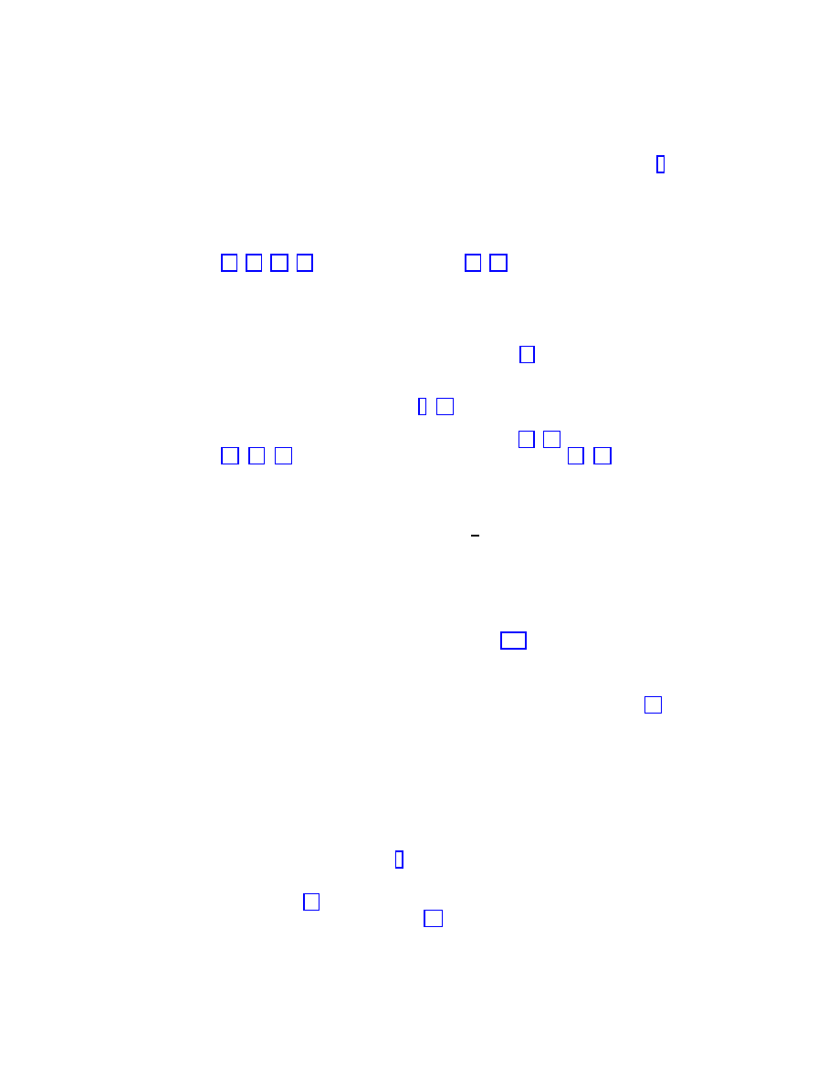
Heisenberg group
Phase space (¯h = 0)
Parameter ¯
h
6= 0
ρ
(p,q)
σ
¯
h
R
2
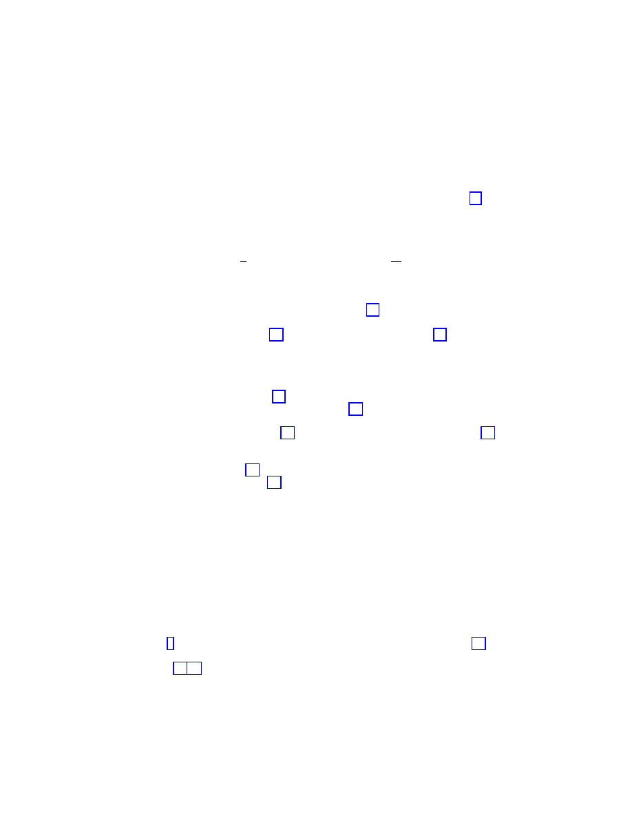
H
Figure 3.
The appearance of both quantum and classic me-
chanics from the same source. Automorphisms of
symplectic group Sp(1) do not mix Schr¨
~
~ and act by the metaplectic representation inside
each of them. In the contrast those automorphisms of
sitively on the set of one dimensional representations ρ
.
In fact Sp(1) is exactly the subgroup of non-inner automorphisms of
H which send
a Shr¨
odinger representation ρ
~
(3.17) with any parameter
~ 6= 0 to an unitary
equivalent representation [16,
§ 1.2].
More precisely for any automorphism α(g), g
∈ Sp(1) of H the composition
ρ
~
◦ α(g) is again a representation, which is unitary equivalent to ρ
~
. Therefore
should exists a unitary operator U (g) in L
2
(
R) such that ρ
~
◦α(g) = U(g)ρ
~
U
−1
(g).
Then the correspondence µ : g
7→ U(g) is a double valued metaplectic representation
of Sp(1) [16,
§ 4.2], [44, § 11.3] in L
2
(
R). We are ready to give our definition of
quantisation.
Definition 5.1. Quantisation
Q is a linear operator from C (R
2
) to B(L
2
(
R)),
which intertwines two actions of the symplectic group Sp(1): by symplectomor-
phisms
R
2
in classical mechanics and the metaplectic representation µ in quantum
mechanics on L
2
(
R):
Qτ(g) = µ(g)Q
forall g
∈ Sp(1).
The following “easy-go” theorem is just an application of several known results
(e.g. [16, Thm. 4.28]) about the metaplectic representation.
Theorem 5.2. [26] The Weyl calculus (4.1) is unique (up to equivalence) well-
defined solution for the quantisation problem 5.1.
It is interesting to note that the quantisation
Q which exactly intertwines sym-
plectomorphisms also approximately intertwines any canonical transformation of
R
2
modulo smoothing operators—this is statement of the important Egorov theo-
rem [43,
§ VIII.1] from the theory of PDO.
One can get even more from our study of automorphism of
H. We recall that the
Heisenberg group
H besides of the family of Schr¨odinger representations σ
~
22
VLADIMIR V. KISIL
with parameter
~ ∈ R \ {0} has only in addition the family of one dimensional
representations ρ
(p,q)
:
ρ
(p,q)
: (s, x, y)
7→ e
i(xp+yq)
,
where
(p, q)
∈ R
2
.
(5.4)
That family is usually just mentioned by accurate authors in the statement of the
Stone-von Neumann theorem [16, 44] but almost never used in any way: what
could we expect interesting from commutative representations in our age of non-
commutative geometry? But let us take a second look assuming that Nature does
not create anything without a purpose.
The representation α (5.3) of Sp(1) could be lifted to the action α
∗
on the
dual object (the set of all unitary irreducible representations) b
H of H. As was
mentioned before each Schr¨
odinger representation σ
~
(3.17) is a fixed point of α
∗
.
In the contrast the whole family of one dimensional representations ρ
: it acts transitively on the set (p, q) by symplectomorphisms (5.2).
Therefore it is natural to identify the family of representation (5.4) with the phase
space. This situation is illustrated by Figure 3. From the topology on the dual
object b
H [20, § 7.2.2] the correct place to put the entire family (5.4) is the point
~ = 0. Moreover representations σ
~
,
~ 6= 0 are dense in R
2
—this is a form of the
correspondence principle between quantum and classical mechanics. Reader may
wish to compare our Figure 3 with Figs. 6 and 7 in [20,
§ 7.2.2] and corresponding
discussion there of topology on b
H. It is slightly speculative but we could also assume
that negative values of
~ on bH correspond to anti-particles because the minus sign
of
~ reverses the time flow in the Schr¨odinger equation.
How far could that relation between quantum and classic mechanics be extend?
It turns that we can introduce an appropriate notion of dynamics [27] on
H which
produces quantum and classical dynamics in corresponding representations (3.17)
and (5.4). That unified dynamics is based on the following definition.
Definition 5.3. [27] The p-mechanical brackets of two functions k
1
(s, x, y),
k
2
(s, x, y) on the Heisenberg group
H are defined as follows:
{[k
1
, k
2
]
} = A(k
1
∗ k
2
− k
2
∗ k
1
),
(5.5)
where
∗ denotes the group convolution on H of two functions and A acts as anti-
derivative with respect of the variable s.
The main property of p-mechanical brackets is a common source for quantum
and classical brackets:
Proposition 5.4. [27] The images of p-mechanical brackets (5.5) under infi-
nite dimensional representations σ
~
(3.17),
~ 6= 0 and finite dimensional represen-
tations ρ
(q,p)
(5.4) are quantum commutator and Poisson brackets of functions ˆ
k
1
and ˆ
k
2
respectively:
ρ(
{[k
1
, k
2
]
}) =
1
i
~
[ˆ
k
1
, ˆ
k
2
] =
1
i
~
(K
1
K
2
− K
2
K
1
),
ρ = σ
~
,
~ 6= 0;
{ˆk
1
, ˆ
k
2
} =
∂ˆ
k
1
∂q
∂ˆ
k
2
∂p
−
∂ˆ
k
1
∂p
∂ˆ
k
2
∂q
,
ρ = ρ
(q,p)
.
(5.6)
We refer to the paper [27] for further details and discussion about the p-
mechanical brackets, dynamics generated by them and its relations to quantum
and classical mechanics. It convinces that not only quantum mechanics but classi-
cal too appear from representations of the Heisenberg group.
DESCARTES AND KLEIN ON NONCOMMUTATIVE GEOMETRY
23
Conclusion
A mathematical idea should not be petrified in a formalised
axiomatic settings, but should be considered instead as
flowing as a river.
Sylvester 1878
It is accurate to say that the idea of symmetries and invariants was dominant
and the most fruitful in the physics of XX century. There is no a contradiction
however to hope that its systematical use will reveal many secrets and explain
many mysteries of the Nature in the future as well. That idea is among very few
other which are strong enough to oppose a collapse of science into many unrelated
parts. Moreover the admiration of symmetries is common to both cultures (in the
sense of C.P. Snow) and could be a bridge between them.
Acknowledgments
I am grateful to the editors who published my previous paper [24] on that topic
despite of the obvious doubts it generated.
References
[1] Syed Twareque Ali, Jean-Pierre Antoine, and Jean-Pierre Gazeau. Coherent States, Wavelets
and Their Generalizations. Graduate Texts in Contemporary Physics. Springer-Verlag, New
York, 2000. 3, 3.4
[2] Robert F.V. Anderson. The Weyl functional calculus. J. Funct. Anal., 4:240–267, 1969. 4, 4
[3] V. I. Arnol’d. On the teaching of mathematics. Uspekhi Mat. Nauk, 53(1(319)):229–234, 1998.
MR # 99k:00011. E-print: http://www.botik.ru/~duzhin/as/arnold/oprep fr.ps.gz. 1
[4] Vladimir I. Arnold. Mathematical Methods of Classic Mechanics. Springer-Verlag, Berlin,
1991. 5
[5] Michael Atiyah and Wilfried Schmid. A geometric construction of the discrete series for
semisimple Lie group. In J.A. Wolf, M. Cahen, and M. De Wilde, editors, Harmonic Analysis
and Representations of Semisimple Lie Group, volume 5 of Mathematical Physics and Applied
Mathematics, pages 317–383. D. Reidel Publishing Company, Dordrecht, Holland, 1980. 3.7
[6] V. Bargmann. On a Hilbert space of analytic functions and an associated integral transform.
Part I. Comm. Pure Appl. Math., 3:215–228, 1961. (b), (b)
[7] Felix A. Berezin. Method of Second Quantization. “Nauka”, Moscow, 1988. (b), (c)
[8] Pierre Cartier. A mad day’s work: from Grothendieck to Connes and Kontsevich. The evolu-
tion of concepts of space and symmetry [in les relations entre les math´
ematiques et la physique
th´
eorique, 23–42, Inst. Hautes ´
Etudes Sci., Bures-sur-Yvette, 1998; MR # 2000c:01028] (elec-
tronic). Bull. Amer. Math. Soc. (N.S.), 38(4):389–408, 2001. Translated from the French by
Roger Cooke. MR # 1848254. 2, 2
[9] Lewis A. Coburn. Berezin-Toeplitz quantization. In Algebraic Mettods in Operator Theory,
pages 101–108. Birkh¨
auser Verlag, New York, 1994. (b)
[10] Alain Connes. Non-Commutative Geometry. Academic Press, New York, 1994. 41
[11] Alain Connes. Noncommutative geometry—year 2000. Geom. Funct. Anal., (Special Vol-
ume, Part II):481–559, 2000. GAFA 2000 (Tel Aviv, 1999). MR # 1826266. E-print:
arXiv:math.QA/0011193
[12] Alain Connes and Henri Moscovici. The L
2
-index theorem for homogeneous spaces of Lie
groups. Ann. of Math., 115(2):291–330, 1982. (b)
[13] Richard Delanghe, Frank Sommen, and Vladimir Souˇ
cek. Clifford Algebra and Spinor-Valued
Functions. Kluwer Academic Publishers, Dordrecht, 1992. (d), (d)
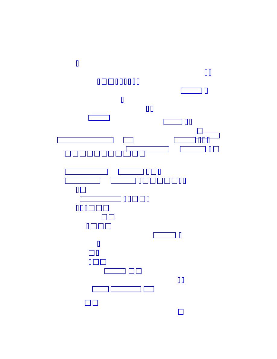
24
VLADIMIR V. KISIL
[14] P.A.M. Dirac. The mathematical foundation of quantum theory. In A. R. Marlow, editor,
Mathematical Foundations of Quantum Theory, pages 1–8. Academic Press, Inc., New York,
1978. 5
[15] Nelson Dunford and Jacob T. Schwartz. Linears Operators. Part I: General Theory, volume
VII of Pure and Applied Mathematics. John Wiley & Sons, Inc., New York, 1957. 4, 4
[16] Gerald B. Folland. Harmonic Analysis in Phase Space. Princeton University Press, Princeton,
New Jersey, 1989. 3, (c), (c), 4, 5, 5, 5, 5, 5
[17] Roger A. Horn and Charles R. Johnson. Topics in Matrix Analysis. Cambridge University
Press, Cambridge, 1994. Corrected reprint of the 1991 original. MR # 95c:15001. 4
[18] Roger Howe. On the role of the Heisenberg group in harmonic analysis. Bull. Amer. Math.
Soc. (N.S.), 3(2):821–843, 1980. 3
[19] Roger Howe and Eng Chye Tan. Non-Abelian Harmonic Analysis: Applications of SL(2,
R).
Universitext. Springer-Verlag, New York, 1992. 3, 3
[20] A. A. Kirillov. Introduction to the theory of representations and noncommutative harmonic
analysis [MR # 90a:22005]. In Representation Theory and Noncommutative Harmonic Anal-
ysis, I, pages 1–156, 227–234. Springer, Berlin, 1994. MR # 1311488. 5, 5
[21] Alexander A. Kirillov. Elements of the Theory of Representations, volume 220 of A Series
of Comprehensive Studies in Mathematics. Springer-Verlag, New York, 1976. 3.1
[22] Vladimir V. Kisil. M¨
obius transformations and monogenic functional calculus. Electron. Res.
Announc. Amer. Math. Soc., 2(1):26–33, 1996. (electronic) MR # 98a:47018. 2, 4, 4
[23] Vladimir V. Kisil. Analysis in
R
1,1
or the principal function theory. Complex Variables Theory
Appl., 40(2):93–118, 1999. E-print: arXiv:funct-an/9712003. MR # 2000k:30078. 2, 3.1,
(d), (d), (d), (c), (c), 3.8, (c), (d), 3.11, (d), 3.4
[24] Vladimir V. Kisil. Two approaches to non-commutative geometry. In H. Begehr,
O. Celebi, and W. Tutschke, editors, Complex Methods for Partial Differential Equa-
tions, chapter 14, pages 219–248. Kluwer Academic Publishers, Netherlands, 1999. E-print:
arXiv:funct-an/9703001
, MR # 2001a:01002. 2, 3.4, 5
[25] Vladimir V. Kisil. Wavelets in Banach spaces. Acta Appl. Math., 59(1):79–109, 1999. E-print:
. MR # 2001c:43013. 2, 3.1, 3.2, (a), (c), 3.4, 4, 4
[26] Vladimir V. Kisil. P -Mechanics and quantisation as an intertwining operator. In preparation,
[27] Vladimir V. Kisil. Quantum and classic brackets. Int. J. Theor. Phys., 41(1):63–77, 2002.
E-print: arXiv:math-ph/0007030. 2, 5, 5.3, 5.4, 5
[28] Vladimir V. Kisil. A spectral decomposition: Invading the third dimension. (In preparation),
[29] A.W. Knapp and N.R. Wallach. Szeg¨
o kernels associated with discrete series. Invent. Math.,
[30] Serge Lang. SL
2
(R), volume 105 of Graduate Text in Mathematics. Springer-Verlag, New
[31] Yu. I. Manin. Mathematics and Physics. Birkh¨
auser Boston, Mass., 1981. Translated from
the Russian by Ann Koblitz and Neal Koblitz. MR # 84m:81003. 3
[32] Yuri I. Manin. Topics in Noncommutative Geometry. Princeton University Press, Princeton,
New Jersey, 1991. 2
[33] Peter J. Olver. Equivalence, invariants, and symmetry. Cambridge University Press, Cam-
[34] A.M. Perelomov. Generalized Coherent States and Their Applications. Springer-Verlag,
[35] Ian R. Porteous. Clifford Algebras and the Classical Groups. Cambridge University Press,
Cambridge, 1995. MR # 97c:15046. (d), (d)
[36] Michael Reed and Barry Simon. Functional Analysis, volume 1 of Methods of Modern Math-
ematical Physics. Academic Press, Orlando, second edition, 1980. 4, 4
[37] I. E. Segal. A non-commutative extension of abstract integration. Ann. of Math. (2), 57:401–
457, 1953. MR # 14:991f, JSTOR collection. 2.0(2)
[38] Irving E. Segal. Mathematical Problems of Relativistic Physics, volume II of Proceedings of the
Summer Seminar (Boulder, Colorado, 1960). American Mathematical Society, Providence,
R.I., 1963. (b), (b)
[39] Irving E. Segal. Mathematical Cosmology and Extragalactic Astronomy, volume 68 of Pure
and Applied Mathematics. Academic Press, Inc., New York, 1986. (d)
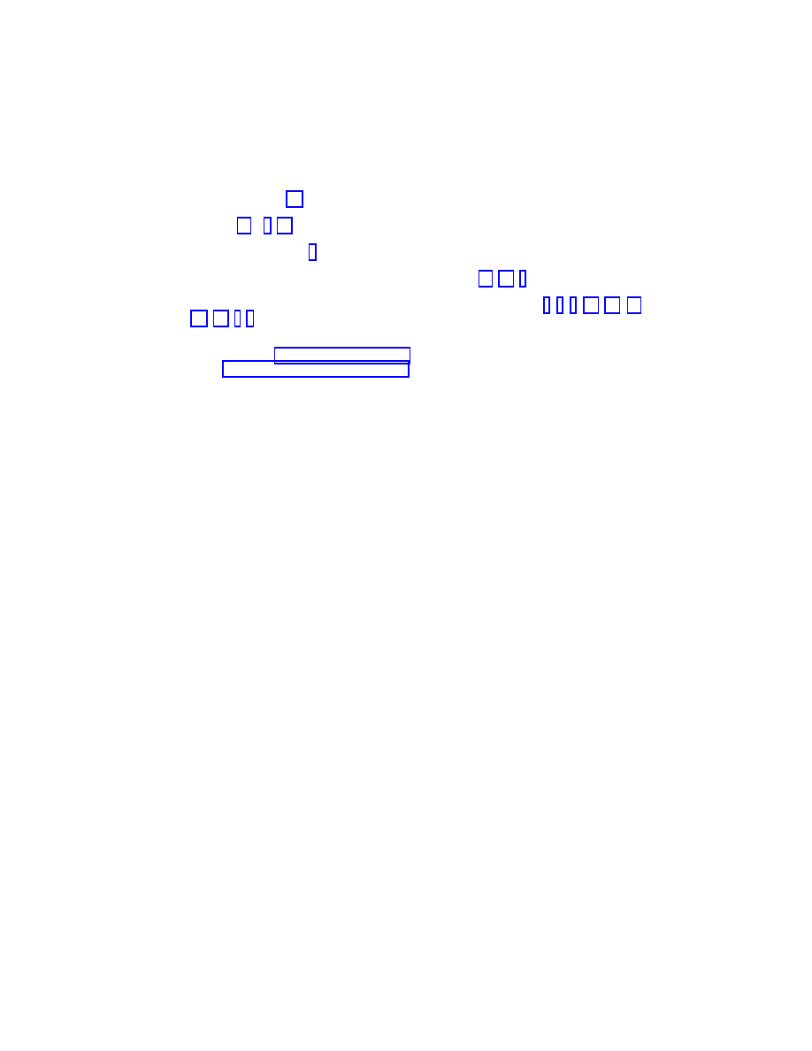
DESCARTES AND KLEIN ON NONCOMMUTATIVE GEOMETRY
25
[40] Irving E. Segal. Algebraic quantization and stability. In William B. Arveson and Ronald G.
Douglas, editors, Operator Theory: Operator Algebras and Applications, number 51 in Pro-
ceedings of Symposia in Mathematics, pages 503–518. American Mathematical Society, Prov-
idence, R.I., 1990. (a)
[41] Irving E. Segal. Book review. Bull. Amer. Math. Soc. (N.S.), 33(4):459–465, 1996. Review
[42] Joseph L. Taylor. The analytic-functional calculus for several commuting operators. Acta
Math., 125:1–38, 1970. 4
[43] Michael E. Taylor. Pseudodifferential Operators, volume 34 of Princeton Mathematical Series.
Princeton University Press, Princeton, New Jersey, 1981. (c), (c), 5
[44] Michael E. Taylor. Noncommutative Harmonic Analysis, volume 22 of Math. Surv. and
Monographs. American Mathematical Society, Providence, R.I., 1986. 3, 3, 3, (a), (a), (c),
(d), (d), 5, 5
School of Mathematics, University of Leeds, Leeds LS2 9JT, UK
E-mail address : kisilv@maths.leeds.ac.uk
URL: http://maths.leeds.ac.uk/~kisilv/
Wyszukiwarka
Podobne podstrony:
więcej podobnych podstron