
arXiv:quant-ph/0101012 v4 25 Sep 2001
Quantum Theory From Five Reasonable Axioms
Lucien Hardy
∗
Centre for Quantum Computation,
The Clarendon Laboratory,
Parks road, Oxford OX1 3PU, UK
September 25, 2001
Abstract
The usual formulation of quantum theory is based on
rather obscure axioms (employing complex Hilbert
spaces, Hermitean operators, and the trace formula
for calculating probabilities).
In this paper it is
shown that quantum theory can be derived from five
very reasonable axioms. The first four of these ax-
ioms are obviously consistent with both quantum the-
ory and classical probability theory. Axiom 5 (which
requires that there exist continuous reversible trans-
formations between pure states) rules out classical
probability theory. If Axiom 5 (or even just the word
“continuous” from Axiom 5) is dropped then we ob-
tain classical probability theory instead. This work
provides some insight into the reasons why quantum
theory is the way it is. For example, it explains the
need for complex numbers and where the trace for-
mula comes from. We also gain insight into the rela-
tionship between quantum theory and classical prob-
ability theory.
1
Introduction
Quantum theory, in its usual formulation, is very ab-
stract. The basic elements are vectors in a complex
Hilbert space. These determine measured probabil-
ities by means of the well known trace formula - a
formula which has no obvious origin. It is natural to
ask why quantum theory is the way it is. Quantum
∗
hardy@qubit.org.
This is version 4
theory is simply a new type of probability theory.
Like classical probability theory it can be applied
to a wide range of phenomena. However, the rules
of classical probability theory can be determined by
pure thought alone without any particular appeal to
experiment (though, of course, to develop classical
probability theory, we do employ some basic intu-
itions about the nature of the world). Is the same
true of quantum theory? Put another way, could a
19th century theorist have developed quantum the-
ory without access to the empirical data that later
became available to his 20th century descendants?
In this paper it will be shown that quantum theory
follows from five very reasonable axioms which might
well have been posited without any particular access
to empirical data. We will not recover any specific
form of the Hamiltonian from the axioms since that
belongs to particular applications of quantum the-
ory (for example - a set of interacting spins or the
motion of a particle in one dimension). Rather we
will recover the basic structure of quantum theory
along with the most general type of quantum evo-
lution possible. In addition we will only deal with
the case where there are a finite or countably infinite
number of distinguishable states corresponding to a
finite or countably infinite dimensional Hilbert space.
We will not deal with continuous dimensional Hilbert
spaces.
The basic setting we will consider is one in which
we have preparation devices, transformation devices,
and measurement devices.
Associated with each
preparation will be a state defined in the following
1

way:
The state associated with a particular preparation
is defined to be (that thing represented by) any
mathematical object that can be used to deter-
mine the probability associated with the out-
comes of any measurement that may be per-
formed on a system prepared by the given prepa-
ration.
Hence, a list of all probabilities pertaining to all pos-
sible measurements that could be made would cer-
tainly represent the state. However, this would most
likely over determine the state. Since most physical
theories have some structure, a smaller set of prob-
abilities pertaining to a set of carefully chosen mea-
surements may be sufficient to determine the state.
This is the case in classical probability theory and
quantum theory. Central to the axioms are two inte-
gers K and N which characterize the type of system
being considered.
• The number of degrees of freedom, K, is defined
as the minimum number of probability measure-
ments needed to determine the state, or, more
roughly, as the number of real parameters re-
quired to specify the state.
• The dimension, N , is defined as the maximum
number of states that can be reliably distin-
guished from one another in a single shot mea-
surement.
We will only consider the case where the number
of distinguishable states is finite or countably infi-
nite. As will be shown below, classical probability
theory has K = N and quantum probability theory
has K = N
2
(note we do not assume that states are
normalized).
The five axioms for quantum theory (to be stated
again, in context, later) are
Axiom 1 Probabilities. Relative frequencies (mea-
sured by taking the proportion of times a par-
ticular outcome is observed) tend to the same
value (which we call the probability) for any case
where a given measurement is performed on a
ensemble of n systems prepared by some given
preparation in the limit as n becomes infinite.
Axiom 2 Simplicity. K is determined by a function
of N (i.e. K = K(N )) where N = 1, 2, . . . and
where, for each given N , K takes the minimum
value consistent with the axioms.
Axiom 3 Subspaces. A system whose state is con-
strained to belong to an M dimensional subspace
(i.e. have support on only M of a set of N possi-
ble distinguishable states) behaves like a system
of dimension M .
Axiom 4 Composite systems. A composite system
consisting of subsystems A and B satisfies N =
N
A
N
B
and K = K
A
K
B
Axiom 5 Continuity. There exists a continuous re-
versible transformation on a system between any
two pure states of that system.
The first four axioms are consistent with classical
probability theory but the fifth is not (unless the
word “continuous” is dropped). If the last axiom is
dropped then, because of the simplicity axiom, we
obtain classical probability theory (with K = N ) in-
stead of quantum theory (with K = N
2
). It is very
striking that we have here a set of axioms for quan-
tum theory which have the property that if a single
word is removed – namely the word “continuous” in
Axiom 5 – then we obtain classical probability theory
instead.
The basic idea of the proof is simple. First we show
how the state can be described by a real vector, p,
whose entries are probabilities and that the probabil-
ity associated with an arbitrary measurement is given
by a linear function, r
· p, of this vector (the vector r
is associated with the measurement). Then we show
that we must have K = N
r
where r is a positive in-
teger and that it follows from the simplicity axiom
that r = 2 (the r = 1 case being ruled out by Axiom
5). We consider the N = 2, K = 4 case and recover
quantum theory for a two dimensional Hilbert space.
The subspace axiom is then used to construct quan-
tum theory for general N . We also obtain the most
general evolution of the state consistent with the ax-
ioms and show that the state of a composite system
can be represented by a positive operator on the ten-
sor product of the Hilbert spaces of the subsystems.
2

Finally, we show obtain the rules for updating the
state after a measurement.
This paper is organized in the following way.
First we will describe the type of situation we wish
to consider (in which we have preparation devices,
state transforming devices, and measurement de-
vices). Then we will describe classical probability
theory and quantum theory. In particular it will be
shown how quantum theory can be put in a form sim-
ilar to classical probability theory. After that we will
forget both classical and quantum probability theory
and show how they can be obtained from the axioms.
Various authors have set up axiomatic formula-
tions of quantum theory, for example see references
[1, 2, 3, 4, 5, 6, 7, 8, 9, 10] (see also [11, 12, 13]).
Much of this work is in the quantum logic tradition.
The advantage of the present work is that there are
a small number of simple axioms, these axioms can
easily be motivated without any particular appeal to
experiment, and the mathematical methods required
to obtain quantum theory from these axioms are very
straightforward (essentially just linear algebra).
2
Setting the Scene
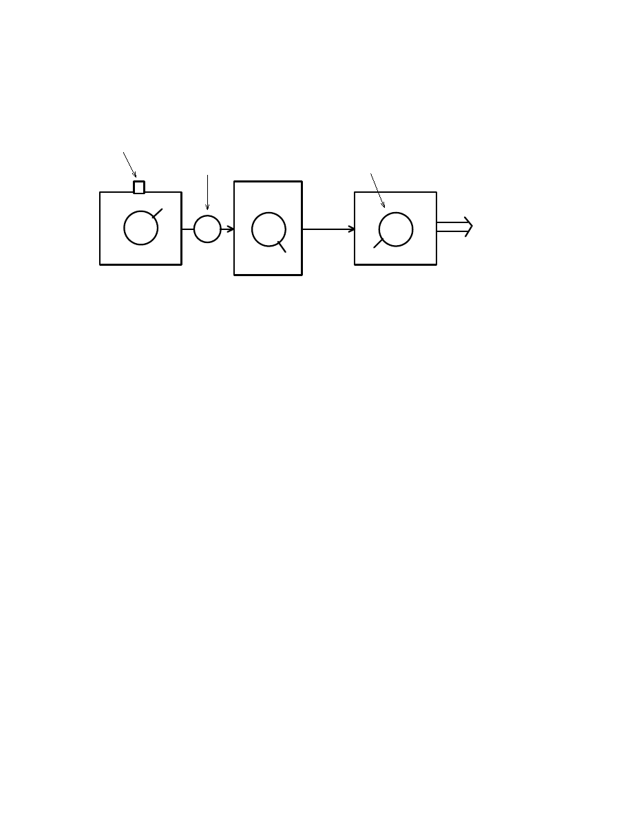
We will begin by describing the type of experimen-
tal situation we wish to consider (see Fig. 1). An
experimentalist has three types of device. One is a
preparation device. We can think of it as preparing
physical systems in some state. It has on it a num-
ber of knobs which can be varied to change the state
prepared. The system is released by pressing a but-
ton. The system passes through the second device.
This device can transform the state of the system.
This device has knobs on it which can be adjusted
to effect different transformations (we might think of
these as controlling fields which effect the system).
We can allow the system to pass through a number
of devices of this type. Unless otherwise stated, we
will assume the transformation devices are set to al-
low the system through unchanged. Finally, we have
a measurement apparatus. This also has knobs on it
which can be adjusted to determine what measure-
ment is being made. This device outputs a classical
number. If no system is incident on the device (i.e.
because the button on the preparation device was
not pressed) then it outputs a 0 (corresponding to a
null outcome). If there is actually a physical system
incident (i.e when the release button is pressed and
the transforming device has not absorbed the system)
then the device outputs a number l where l = 1 to L
(we will call these non-null outcomes). The number
of possible classical outputs, L, may depend on what
is being measured (the settings of the knobs).
The fact that we allow null events means that we
will not impose the constraint that states are nor-
malized. This turns out to be a useful convention.
It may appear that requiring the existence of null
events is an additional assumption. However, it fol-
lows from the subspace axiom that we can arrange to
have a null outcome. We can associate the non-null
outcomes with a certain subspace and the null out-
come with the complement subspace. Then we can
restrict ourselves to preparing only mixtures of states
which are in the non-null subspace (when the button
is pressed) with states which are in the null subspace
(when the button is not pressed).
The situation described here is quite generic. Al-
though we have described the set up as if the system
were moving along one dimension, in fact the system
could equally well be regarded as remaining station-
ary whilst being subjected to transformations and
measurements. Furthermore, the system need not be
localized but could be in several locations. The trans-
formations could be due to controlling fields or simply
due to the natural evolution of the system. Any phys-
ical experiment, quantum, classical or other, can be
viewed as an experiment of the type described here.
3
Probability measurements
We will consider only measurements of probability
since all other measurements (such as expectation
values) can be calculated from measurements of prob-
ability. When, in this paper, we refer to a measure-
ment or a probability measurement we mean, specifi-
cally, a measurement of the probability that the out-
come belongs to some subset of the non-null outcomes
with a given setting of the knob on the measurement
apparatus. For example, we could measure the prob-
3
Release button
System
Preparation
Transformation
Measurement
Classical
information
out
Knob
Figure 1: The situation considered consists of a preparation device with a knob for varying the state of the
system produced and a release button for releasing the system, a transformation device for transforming the
state (and a knob to vary this transformation), and a measuring apparatus for measuring the state (with a
knob to vary what is measured) which outputs a classical number.
ability that the outcome is l = 1 or l = 2 with some
given setting.
To perform a measurement we need a large number
of identically prepared systems.
A measurement returns a single real number (the
probability) between 0 and 1. It is possible to per-
form many measurements at once. For example, we
could simultaneously measure [the probability the
outcome is l = 1] and [the probability the outcome is
l = 1 or l = 2] with a given knob setting.
4
Classical Probability Theory
A classical system will have available to it a number,
N , of distinguishable states. For example, we could
consider a ball that can be in one of N boxes. We
will call these distinguishable states the basis states.
Associated with each basis state will be the probabil-
ity, p
n
, of finding the system in that state if we make
a measurement. We can write
p =
p
1
p
2
p
3
..
.
p
N
(1)
This vector can be regarded as describing the state
of the system. It can be determined by measuring
N probabilities and so K = N . Note that we do
not assume that the state is normalized (otherwise
we would have K = N
− 1).
The state p will belong to a convex set S. Since the
set is convex it will have a subset of extremal states.
These are the states
p
1
=
1
0
0
..
.
0
p
2
=
0
1
0
..
.
0
p
3
=
0
0
1
..
.
0
etc.
(2)
4

and the state
p
null
= 0 =
0
0
0
..
.
0
(3)
The state 0 is the null state (when the system is not
present). We define the set of pure states to consist of
all extremal states except the null state. Hence, the
states in (2) are the pure states. They correspond to
the system definitely being in one of the N distin-
guishable states. A general state can be written as
a convex sum of the pure states and the null state
and this gives us the exact form of the set S. This is
always a polytope (a shape having flat surfaces and
a finite number of vertices).
We will now consider measurements. Consider a
measurement of the probability that the system is in
the basis state n. Associated with this probability
measurement is the vector r
n
having a 1 in position
n and 0’s elsewhere. At least for these cases the mea-
sured probability is given by
p
meas
= r
· p
(4)
However, we can consider more general types of prob-
ability measurement and this formula will still hold.
There are two ways in which we can construct more
general types of measurement:
1. We can perform a measurement in which we
decide with probability λ to measure r
A
and
with probability 1
− λ to measure r
B
. Then
we will obtain a new measurement vector r =
λr
A
+ (1
− λ)r
B
.
2. We can add the results of two compatible prob-
ability measurements and therefore add the cor-
responding measurement vectors.
An example of the second is the probability measure-
ment that the state is basis state 1 or basis state 2 is
given by the measurement vector r
1
+ r
2
. From lin-
earity, it is clear that the formula (4) holds for such
more general measurements.
There must exist a measurement in which we sim-
ply check to see that the system is present (i.e. not
in the null state). We denote this by r
I
. Clearly
r
I
=
X
n
r
n
=
1
1
1
..
.
1
(5)
Hence 0
≤ r
I
.p
≤ 1 with normalized states saturat-
ing the upper bound.
With a given setting of the knob on the measure-
ment device there will be a certain number of distinct
non-null outcomes labeled l = 1 to L. Associated
with each outcome will be a measurement vector r
l
.
Since, for normalized states, one non-null outcome
must happen we have
L
X
l=1
r
l
= r
I
(6)
This equation imposes a constraint on any measure-
ment vector. Let allowed measurement vectors r be-
long to the set R. This set is clearly convex (by virtue
of 1. above). To fully determine R first consider the
set R
+
consisting of all vectors which can be written
as a sum of the basis measurement vectors, r
n
, each
multiplied by a positive number. For such vectors
r
· p is necessarily greater than 0 but may also be
greater than 1. Thus, elements of R
+
may be too
long to belong to R. We need a way of picking out
those elements of R
+
that also belong to R. If we
can perform the probability measurement r then, by
(6) we can also perform the probability measurement
r
≡ r
I
− r. Hence,
Iff
r, r
∈ R
+
and r + r = r
I
then
r, r
∈ R
(7)
This works since it implies that r
· p ≤ 1 for all p so
that r is not too long.
Note that the Axioms 1 to 4 are satisfied but Axiom
5 is not since there are a finite number of pure states.
It is easy to show that reversible transformations take
pure states to pure states (see Section 7). Hence a
5

continuous reversible transformation will take a pure
state along a continuous path through the pure states
which is impossible here since there are only a finite
number of pure states.
5
Quantum Theory
Quantum theory can be summarized by the following
rules
States The state is represented by a positive (and
therefore Hermitean) operator ˆ
ρ satisfying 0
≤
tr(ˆ
ρ)
≤ 1.
Measurements Probability measurements are rep-
resented by a positive operator ˆ
A. If ˆ
A
l
corre-
sponds to outcome l where l = 1 to L then
L
X
l=1
ˆ
A
l
= ˆ
I
(8)
Probability formula The
probability
obtained
when the measurement ˆ
A is made on the state
ˆ
ρ is
p
meas
= tr( ˆ
Aˆ
ρ)
(9)
Evolution The most general evolution is given by
the superoperator $
ˆ
ρ
→ $(ρ)
(10)
where $
• Does not increase the trace.
• Is linear.
• Is completely positive.
This way of presenting quantum theory is rather con-
densed.
The following notes should provide some
clarifications
1. It is, again, more convenient not to impose nor-
malization. This, in any case, more accurately
models what happens in real experiments when
the quantum system is often missing for some
portion of the ensemble.
2. The most general type of measurement in quan-
tum theory is a POVM (positive operator valued
measure). The operator ˆ
A is an element of such
a measure.
3. Two classes of superoperator are of particular
interest. If $ is reversible (i.e. the inverse $
−1
both exists and belongs to the allowed set of
transformations) then it will take pure states
to pure states and corresponds to unitary evo-
lution. The von Neumann projection postulate
takes the state ˆ
ρ to the state ˆ
P ˆ
ρ ˆ
P when the out-
come corresponds to the projection operator ˆ
P .
This is a special case of a superoperator evolu-
tion in which the trace of ˆ
ρ decreases.
4. It has been shown by Krauss [14] that one need
only impose the three listed constraints on $ to
fully constrain the possible types of quantum
evolution. This includes unitary evolution and
von Neumann projection as already stated, and
it also includes the evolution of an open system
(interacting with an environment). It is some-
times stated that the superoperator should pre-
serve the trace. However, this is an unnecessary
constraint which makes it impossible to use the
superoperator formalism to describe von Neu-
mann projection [15].
5. The constraint that $ is completely positive im-
poses not only that $ preserves the positivity of
ˆ
ρ but also that $
A
⊗ ˆ
I
B
acting on any element of
a tensor product space also preserves positivity
for any dimension of B.
This is the usual formulation. However, quantum
theory can be recast in a form more similar to classi-
cal probability theory. To do this we note first that
the space of Hermitean operators which act on a N
dimensional complex Hilbert space can be spanned
by N
2
linearly independent projection operators ˆ
P
k
for k = 1 to K = N
2
. This is clear since a general
Hermitean operator can be represented as a matrix.
This matrix has N real numbers along the diagonal
and
1
2
N (N
− 1) complex numbers above the diago-
nal making a total of N
2
real numbers. An example
of N
2
such projection operators will be given later.
6

Define
ˆ
P =
ˆ
P
1
ˆ
P
2
..
.
ˆ
P
K
(11)
Any Hermitean matrix can be written as a sum of
these projection operators times real numbers, i.e. in
the form a
· ˆ
P where a is a real vector (a is unique since
the operators ˆ
P
k
are linearly independent). Now de-
fine
p
S
= tr( ˆ
Pˆ
ρ)
(12)
Here the subscript S denotes ‘state’. The kth compo-
nent of this vector is equal to the probability obtained
when ˆ
P
k
is measured on ˆ
ρ. The vector p
S
contains
the same information as the state ˆ
ρ and can therefore
be regarded as an alternative way of representing the
state. Note that K = N
2
since it takes N
2
probabil-
ity measurements to determine p
S
or, equivalently,
ˆ
ρ. We define r
M
through
ˆ
A = r
M
· ˆ
P
(13)
The subscript M denotes ‘measurement’. The vector
r
M
is another way of representing the measurement
ˆ
A. If we substitute (13) into the trace formula (9) we
obtain
p
meas
= r
M
· p
S
(14)
We can also define
p
M
= tr( ˆ
A ˆ
P)
(15)
and r
S
by
ˆ
ρ = ˆ
P
· r
S
(16)
Using the trace formula (9) we obtain
p
meas
= p
M
· r
S
= r
T
M
Dr
S
(17)
where T denotes transpose and D is the K
×K matrix
with real elements given by
D
ij
= tr( ˆ
P
i
ˆ
P
j
)
(18)
or we can write D = tr( ˆ
P ˆ
P
T
). From (14,17) we
obtain
p
S
= Dr
S
(19)
and
p
M
= D
T
r
M
(20)
We also note that
D = D
T
(21)
though this would not be the case had we chosen dif-
ferent spanning sets of projection operators for the
state operators and measurement operators. The in-
verse D
−1
must exist (since the projection operators
are linearly independent). Hence, we can also write
p
meas
= p
T
M
D
−1
p
S
(22)
The state can be represented by an r-type vector or
a p-type vector as can the measurement. Hence the
subscripts M and S were introduced. We will some-
times drop these subscripts when it is clear from the
context whether the vector is a state or measurement
vector. We will stick to the convention of having mea-
surement vectors on the left and state vectors on the
right as in the above formulae.
We define r
I
by
ˆ
I = r
I
· ˆ
P
(23)
This measurement gives the probability of a non-null
event. Clearly we must have 0
≤ r
I
· p ≤ 1 with nor-
malized states saturating the upper bound. We can
also define the measurement which tells us whether
the state is in a given subspace. Let ˆ
I
W
be the pro-
jector into an M dimensional subspace W . Then the
corresponding r vector is defined by ˆ
I
W
= r
I
W
· ˆ
P.
We will say that a state p is in the subspace W if
r
I
W
· p = r
I
· p
(24)
so it only has support in W . A system in which
the state is always constrained to an M -dimensional
subspace will behave as an M dimensional system in
accordance with Axiom 3.
7

The transformation ˆ
ρ
→ $(ˆ
ρ) of ˆ
ρ corresponds to
the following transformation for the state vector p:
p
=
tr( ˆ
Pˆ
ρ)
→ tr( ˆ
P$(ˆ
ρ))
=
tr( ˆ
P$( ˆ
P
T
D
−1
p))
=
Zp
where equations (16,19) were used in the third line
and Z is a K
× K real matrix given by
Z = tr( ˆ
P$( ˆ
P)
T
)D
−1
(25)
(we have used the linearity property of $). Hence, we
see that a linear transformation in ˆ
ρ corresponds to
a linear transformation in p. We will say that Z
∈ Γ.
Quantum theory can now be summarized by the
following rules
States The state is given by a real vector p
∈ S with
N
2
components.
Measurements A measurement is represented by a
real vector r
∈ R with N
2
components.
Probability measurements The measured proba-
bility if measurement r is performed on state p
is
p
meas
= r
· p
Evolution The evolution of the state is given by
p
→ Zp where Z ∈ Γ is a real matrix.
The exact nature of the sets S, R and Γ can be de-
duced from the equations relating these real vectors
and matrices to their counterparts in the usual quan-
tum formulation. We will show that these sets can
also be deduced from the axioms. It has been no-
ticed by various other authors that the state can be
represented by the probabilities used to determine it
[18, 19].
There are various ways of choosing a set of N
2
linearly independent projections operators ˆ
P
k
which
span the space of Hermitean operators. Perhaps the
simplest way is the following. Consider an N dimen-
sional complex Hilbert space with an orthonormal ba-
sis set
|ni for n = 1 to N . We can define N projectors
|nihn|
(26)
Each of these belong to one-dimensional subspaces
formed from the orthonormal basis set. Define
|mni
x
=
1
√
2
(
|mi + |ni)
|mni
y
=
1
√
2
(
|mi + i|ni)
for m < n. Each of these vectors has support on a
two-dimensional subspace formed from the orthonor-
mal basis set.
There are
1
2
N (N
− 1) such two-
dimensional subspaces. Hence we can define N (N
−1)
further projection operators
|mni
x
hmn| and |mni
y
hmn|
(27)
This makes a total of N
2
projectors. It is clear that
these projectors are linearly independent.
Each projector corresponds to one degree of free-
dom.
There is one degree of freedom associated
with each one-dimensional subspace n, and a fur-
ther two degrees of freedom associated with each two-
dimensional subspace mn. It is possible, though not
actually the case in quantum theory, that there are
further degrees of freedom associated with each three-
dimensional subspace and so on. Indeed, in general,
we can write
K
=
N x
1
+
1
2!
N (N
− 1)x
2
+
1
3!
N (N
− 1)(N − 2)x
3
+ . . .
(28)
We will call the vector x = (x
1
, x
2
, . . . ) the signature
of a particular probability theory. Classical proba-
bility theory has signature x
Classical
= (1, 0, 0, . . .)
and quantum theory has signature x
Quantum
=
(1, 2, 0, 0, . . .). We will show that these signatures
are respectively picked out by Axioms 1 to 4 and Ax-
ioms 1 to 5. The signatures x
Reals
= (1, 1, 0, 0, . . .) of
real Hilbert space quantum theory and x
Quaternions
=
(1, 4, 0, 0, . . .) of quaternionic quantum theory are
ruled out.
If we have a composite system consisting of subsys-
tem A spanned by ˆ
P
A
i
(i = 1 to K
A
) and B spanned
by ˆ
P
B
j
(j = 1 to K
B
) then ˆ
P
A
i
⊗ ˆ
P
B
j
are linearly inde-
pendent and span the composite system. Hence, for
the composite system we have K = K
A
K
B
. We also
have N = N
A
N
B
. Therefore Axiom 4 is satisfied.
8

The set S is convex. It contains the null state 0
(if the system is never present) which is an extremal
state. Pure states are defined as extremal states other
than the null state (since they are extremal they can-
not be written as a convex sum of other states as we
expect of pure states). We know that a pure state
can be represented by a normalized vector
|ψi. This
is specified by 2N
− 2 real parameters (N complex
numbers minus overall phase and minus normaliza-
tion). On the other hand, the full set of normalized
states is specified by N
2
− 1 real numbers. The sur-
face of the set of normalized states must therefore be
N
2
− 2 dimensional. This means that, in general, the
pure states are of lower dimension than the the sur-
face of the convex set of normalized states. The only
exception to this is the case N = 2 when the surface
of the convex set is 2-dimensional and the pure states
are specified by two real parameters. This case is il-
lustrated by the Bloch sphere. Points on the surface
of the Bloch sphere correspond to pure states.
In fact the N = 2 case will play a particularly
important role later so we will now develop it a lit-
tle further. There will be four projection operators
spanning the space of Hermitean operators which we
can choose to be
ˆ
P
1
=
|1ih1|
(29)
ˆ
P
2
=
|2ih2|
(30)
ˆ
P
3
= (α
|1i + β|2i)(α
∗
h1| + β
∗
h2|)
(31)
ˆ
P
4
= (γ
|1i + δ|2i)(γ
∗
h1| + δ
∗
h2|)
(32)
where
|α|
2
+
|β|
2
= 1 and
|γ|
2
+
|δ|
2
= 1. We have
chosen the second pair of projections to be more gen-
eral than those defined in (27) above since we will
need to consider this more general case later. We
can calculate D using (18)
D =
1
0
1
− |β|
2
1
− |δ|
2
0
1
|β|
2
|δ|
2
1
− |β|
2
|β|
2
1
|αγ
∗
+ βδ
∗
|
2
1
− |δ|
2
|δ|
2
|αγ
∗
+ βδ
∗
|
2
1
(33)
We can write this as
D =
1
0
1
− a 1 − b
0
1
a
b
1
− a a
1
c
1
− b b
c
1
(34)
where a and b are real with β =
√
a exp(iφ
3
), δ =
√
b exp(φ
4
), and c =
|αγ
∗
+ βδ
∗
|
2
. We can choose α
and γ to be real (since the phase is included in the
definition of β and δ). It then follows that
c = 1
− a − b + 2ab
+2 cos(φ
4
− φ
3
)
p
ab(1
− a)(1 − b)
(35)
Hence, by varying the complex phase associated with
α, β, γ and δ we find that
c
−
< c < c
+
(36)
where
c
±
≡ 1 − a − b + 2ab ± 2
p
ab(1
− a)(1 − b)
(37)
This constraint is equivalent to the condition
Det(D) > 0. Now, if we are given a particular D
matrix of the form (34) then we can go backwards to
the usual quantum formalism though we must make
some arbitrary choices for the phases. First we use
(35) to calculate cos(φ
4
− φ
3
). We can assume that
0
≤ φ
4
− φ
3
≤ π (this corresponds to assigning i to
one of the roots
√
−1). Then we can assume that
φ
3
= 0. This fixes φ
4
. An example of this second
choice is when we assign the state
1
√
2
(
|+i+|−i) (this
has real coefficients) to spin along the x direction for
a spin half particle. This is arbitrary since we have
rotational symmetry about the z axis. Having calcu-
lated φ
3
and φ
4
from the elements of D we can now
calculate α, β, γ, and δ and hence we can obtain ˆ
P.
We can then calculate ˆ
ρ, ˆ
A and $ from p, r, and Z
and use the trace formula. The arbitrary choices for
phases do not change any empirical predictions.
6
Basic Ideas and the Axioms
We will now forget quantum theory and classical
probability theory and rederive them from the ax-
ioms. In this section we will introduce the basic ideas
and the axioms in context.
9

6.1
Probabilities
As mentioned earlier, we will consider only measure-
ments of probability since all other measurements can
be reduced to probability measurements. We first
need to ensure that it makes sense to talk of prob-
abilities. To have a probability we need two things.
First we need a way of preparing systems (in Fig. 1
this is accomplished by the first two boxes) and sec-
ond, we need a way of measuring the systems (the
third box in Fig. 1). Then, we measure the number
of cases, n
+
, a particular outcome is observed when
a given measurement is performed on an ensemble of
n systems each prepared by a given preparation. We
define
prob
+
= lim
n
→∞
n
+
n
(38)
In order for any theory of probabilities to make sense
prob
+
must take the same value for any such infinite
ensemble of systems prepared by a given preparation.
Hence, we assume
Axiom 1 Probabilities. Relative frequencies (mea-
sured by taking the proportion of times a particular
outcome is observed) tend to the same value (which
we call the probability) for any case where a given
measurement is performed on an ensemble of n sys-
tems prepared by some given preparation in the limit
as n becomes infinite.
With this axiom we can begin to build a probability
theory.
Some additional comments are appropriate here.
There are various different interpretations of proba-
bility: as frequencies, as propensities, the Bayesian
approach, etc. As stated, Axiom 1 favours the fre-
quency approach. However, it it equally possible to
cast this axiom in keeping with the other approaches
[16]. In this paper we are principally interested in de-
riving the structure of quantum theory rather than
solving the interpretational problems with probabil-
ity theory and so we will not try to be sophisticated
with regard to this matter. Nevertheless, these are
important questions which deserve further attention.
6.2
The state
We can introduce the notion that the system is de-
scribed by a state. Each preparation will have a state
associated with it. We define the state to be (that
thing represented by) any mathematical object which
can be used to determine the probability for any mea-
surement that could possibly be performed on the
system when prepared by the associated preparation.
It is possible to associate a state with a preparation
because Axiom 1 states that these probabilities de-
pend on the preparation and not on the particular
ensemble being used. It follows from this definition
of a state that one way of representing the state is
by a list of all probabilities for all measurements that
could possibly be performed. However, this would
almost certainly be an over complete specification
of the state since most physical theories have some
structure which relates different measured quantities.
We expect that we will be able to consider a subset
of all possible measurements to determine the state.
Hence, to determine the state we need to make a num-
ber of different measurements on different ensembles
of identically prepared systems. A certain minimum
number of appropriately chosen measurements will be
both necessary and sufficient to determine the state.
Let this number be K. Thus, for each setting, k = 1
to K, we will measure a probability p
k
with an ap-
propriate setting of the knob on the measurement
apparatus. These K probabilities can be represented
by a column vector p where
p =
p
1
p
2
p
3
..
.
p
K
(39)
Now, this vector contains just sufficient information
to determine the state and the state must contain just
sufficient information to determine this vector (other-
wise it could not be used to predict probabilities for
measurements). In other words, the state and this
vector are interchangeable and hence we can use p
as a way of representing the state of the system. We
will call K the number of degrees of freedom associ-
ated with the physical system. We will not assume
10

that the physical system is always present. Hence,
one of the K degrees of freedom can be associated
with normalization and therefore K
≥ 1.
6.3
Fiducial measurements
We will call the probability measurements labeled by
k = 1 to K used in determining the state the fidu-
cial measurements. There is no reason to suppose
that this set is unique. It is possible that some other
fiducial set could also be used to determine the state.
6.4
Measured probabilities
Any probability that can be measured (not just the
fiducial ones) will be determined by some function f
of the state p. Hence,
p
meas
= f(p)
(40)
For different measurements the function will, of
course, be different. By definition, measured prob-
abilities are between 0 and 1.
0
≤ p
meas
≤ 1
This must be true since probabilities are measured by
taking the proportion of cases in which a particular
event happens in an ensemble.
6.5
Mixtures
Assume that the preparation device is in the hands
of Alice. She can decide randomly to prepare a state
p
A
with probability λ or a state p
B
with probability
1
− λ. Assume that she records this choice but does
not tell the person, Bob say, performing the measure-
ment. Let the state corresponding to this preparation
be p
C
. Then the probability Bob measures will be
the convex combination of the two cases, namely
f(p
C
) = λf(p
A
) + (1
− λ)f(p
B
)
(41)
This is clear since Alice could subsequently reveal
which state she had prepared for each event in the
ensemble providing two sub-ensembles. Bob could
then check his data was consistent for each subensem-
ble. By Axiom 1, the probability measured for each
subensemble must be the same as that which would
have been measured for any similarly prepared en-
semble and hence (41) follows.
6.6
Linearity
Equation (41) can be applied to the fiducial measure-
ments themselves. This gives
p
C
= λp
A
+ (1
− λ)p
B
(42)
This is clearly true since it is true by (41) for each
component.
Equations (41,42) give
f(λp
A
+ (1
− λ)p
B
) = λf(p
A
) + (1
− λ)f(p
B
)
(43)
This strongly suggests that the function f(
·) is lin-
ear. This is indeed the case and a proof is given in
Appendix 1. Hence, we can write
p
meas
= r
· p
(44)
The vector r is associated with the measurement.
The kth fiducial measurement is the measurement
which picks out the kth component of p. Hence, the
fiducial measurement vectors are
r
1
=
1
0
0
..
.
0
r
2
=
0
1
0
..
.
0
r
3
=
0
0
1
..
.
0
etc.
(45)
6.7
Transformations
We have discussed the role of the preparation device
and the measurement apparatus. Now we will discuss
the state transforming device (the middle box in Fig.
1). If some system with state p is incident on this
device its state will be transformed to some new state
g(p). It follows from Eqn (41) that this transforma-
tion must be linear. This is clear since we can apply
the proof in the Appendix 1 to each component of g.
Hence, we can write the effect of the transformation
device as
p
→ Zp
(46)
11

where Z is a K
× K real matrix describing the effect
of the transformation.
6.8
Allowed
states,
measurements,
and transformations
We now have states represented by p, measurements
represented by r, and transformations represented by
Z. These will each belong to some set of physically
allowed states, measurements and transformations.
Let these sets of allowed elements be S, R and Γ.
Thus,
p
∈ S
(47)
r
∈ R
(48)
Z
∈ Γ
(49)
We will use the axioms to determine the nature of
these sets. It turns out (for relatively obvious rea-
sons) that each of these sets is convex.
6.9
Special states
If the release button on Fig. 1 is never pressed then
all the fiducial measurements will yield 0. Hence, the
null state p
null
= 0 can be prepared and therefore
0
∈ S.
It follows from (42) that the set S is convex. It is
also bounded since the entries of p are bounded by 0
and 1. Hence, S will have an extremal set S
extremal
(these are the vectors in S which cannot be written
as a convex sum of other vectors in S). We have
0
∈ S
extremal
since the entries in the vectors p cannot
be negative. We define the set of pure states S
pure
to be the set of all extremal states except 0. Pure
states are clearly special in some way. They represent
states which cannot be interpreted as a mixture. A
driving intuition in this work is the idea that pure
states represent definite states of the system.
6.10
The identity measurement
The probability of a non-null outcome is given by
summing up all the non-null outcomes with a given
setting of the knob on the measurement apparatus
(see Fig 1). The non-null outcomes are labeled by
l = 1 to L.
p
non
−null
=
L
X
l=1
r
l
· p = r
I
· p
(50)
where r
l
is the measurement vector corresponding to
outcome l and
r
I
=
L
X
l=1
r
l
(51)
is called the identity measurement.
6.11
Normalized and unnormalized
states
If the release button is never pressed we prepare the
state 0. If the release button is always pressed (i.e
for every event in the ensemble) then we will say
p
∈ S
norm
or, in words, that the state is normalized.
Unnormalized states are of the form λp + (1
− λ)0
where 0
≤ λ < 1. Unnormalized states are therefore
mixtures and hence, all pure states are normalized,
that is
S
pure
⊂ S
norm
We define the normalization coefficient of a state
p to be
µ = r
I
· p
(52)
In the case where p
∈ S
norm
we have µ = 1.
The normalization coefficient is equal to the pro-
portion of cases in which the release button is pressed.
It is therefore a property of the state and cannot de-
pend on the knob setting on the measurement ap-
paratus. We can see that r
I
must be unique since
if there was another such vector satisfying (52) then
this would reduce the number of parameters required
to specify the state contradicting our starting point
that a state is specified by K real numbers. Hence r
I
is independent of the measurement apparatus knob
setting.
12

6.12
Basis states
Any physical system can be in various states. We
expect there to exist some sets of normalized states
which are distinguishable from one another in a sin-
gle shot measurement (were this not the case then we
could store fixed records of information in such phys-
ical systems). For such a set we will have a setting
of the knob on the measurement apparatus such that
each state in the set always gives rise to a particu-
lar outcome or set of outcomes which is disjoint from
the outcomes associated with the other states. It is
possible that there are some non-null outcomes of the
measurement that are not activated by any of these
states. Any such outcomes can be added to the set
of outcomes associated with, say, the first member of
the set without effecting the property that the states
can be distinguished. Hence, if these states are p
n
and the measurements that distinguish them are r
n
then we have
r
m
· p
n
= δ
mn
where
X
n
r
n
= r
I
(53)
The measurement vectors r
n
must add to r
I
since
they cover all possible outcomes. There may be many
such sets having different numbers of elements. Let N
be the maximum number of states in any such set of
distinguishable states. We will call N the dimension.
We will call the states p
n
in any such set basis states
and we will call the corresponding measurements r
n
basis measurements. Each type of physical system
will be characterized by N and K. A note on no-
tation: In general we will adopt the convention that
the subscript n (n = 1 to N ) labels basis states and
measurements and the superscript k (k = 1 to K)
labels fiducial measurements and (to be introduced
later) fiducial states. Also, when we need to work
with a particular choice of fiducial measurements (or
states) we will take the first n of them to be equal to
a basis set. Thus, r
k
= r
k
for k = 1 to N .
If a particular basis state is impure then we can
always replace it with a pure state. To prove this we
note that if the basis state is impure we can write it
as a convex sum of pure states. If the basis state is
replaced by any of the states in this convex sum this
must also satisfy the basis property. Hence, we can
always choose our basis sets to consist only of pure
states and we will assume that this has been done in
what follows.
Note that N = 1 is the smallest value N can take
since we can always choose any normalized state as
p
1
and r
1
= r
I
.
6.13
Simplicity
There will be many different systems having different
K and N . We will assume that, nevertheless, there
is a certain constancy in nature such that K is a
function of N . The second axiom is
Axiom 2 Simplicity. K is determined by a func-
tion of N (i.e. K = K(N )) where N = 1, 2, . . . and
where, for any given N , K takes the minimum value
consistent with the axioms.
The assumption that N = 1, 2, . . . means that we as-
sume nature provides systems of all different dimen-
sions. The motivation for taking the smallest value
of K for each given N is that this way we end up
with the simplest theory consistent with these natu-
ral axioms. It will be shown that the axioms imply
K = N
r
where r is an integer. Axiom 2 then dictates
that we should take the smallest value of r consistent
with the axioms (namely r = 2). However, it would
be interesting either to show that higher values of
r are inconsistent with the axioms even without this
constraint that K should take the minimum value, or
to explicitly construct theories having higher values
of r and investigate their properties.
6.14
Subspaces
Consider a basis measurement set r
n
. The states in a
basis are labeled by the integers n = 1 to N . Consider
a subset W of these integers. We define
r
I
W
=
X
n
∈W
r
n
(54)
Corresponding to the subset W is a subspace which
we will also call W defined by
p
∈ W
iff
r
I
W
· p = r
I
· p
(55)
13

Thus, p belongs to the subspace if it has support
only in the subspace. The dimension of the subspace
W is equal to the number of members of the set W .
The complement subset W consists of the the integers
n = 1 to N not in W . Corresponding to the subset
W is the subspace W which we will call the com-
plement subspace to W . Note that this is a slightly
unusual usage of the terminology “subspace” and “di-
mension” which we employ here because of the anal-
ogous concepts in quantum theory. The third axiom
concerns such subspaces.
Axiom 3 Subspaces. A system whose state is con-
strained to belong to an M dimensional subspace be-
haves like a system of dimension M .
This axiom is motivated by the intuition that any col-
lection of distinguishable states should be on an equal
footing with any other collection of the same number
distinguishable states. In logical terms, we can think
of distinguishable states as corresponding to a propo-
sitions. We expect a probability theory pertaining to
M propositions to be independent of whether these
propositions are a subset or some larger set or not.
One application of the subspace axiom which we
will use is the following: If a system is prepared in
a state which is constrained to a certain subspace W
having dimension N
W
and a measurement is made
which may not pertain to this subspace then this
measurement must be equivalent (so far as measured
probabilities on states in W are concerned) to some
measurement in the set of allowed measurements for
a system actually having dimension N
W
.
6.15
Composite systems
It often happens that a preparation device ejects its
system in such a way that it can be regarded as being
made up of two subsystems. For example, it may emit
one system to the left and one to the right (see Fig.
2). We will label these subsystems A and B. We
assume
Axiom 4 Composite systems. A composite system
consisting of two subsystems A and B having di-
mension N
A
and N
B
respectively, and number of de-
grees of freedom K
A
and K
B
respectively, has dimen-
sion N = N
A
N
B
and number of degrees of freedom
K = K
A
K
B
.
We expect that N = N
A
N
B
for the following rea-
sons. If subsystems A and B have N
A
and N
B
dis-
tinguishable states, then there must certainly exist
N
A
N
B
distinguishable states for the whole system.
It is possible that there exist more than this but we
assume that this is not so. We will show that the
relationship K = K
A
K
B
follows from the following
two assumptions
• If a subsystem is in a pure state then any joint
probabilities between that subsystem and any
other subsystem will factorize. This is a reason-
able assumption given the intuition (mentioned
earlier) that pure states represent definite states
for a system and therefore should not be corre-
lated with anything else.
• The number of degrees of freedom associated
with the full class of states for the composite
system is not greater than the number of degrees
of freedom associated with the separable states.
This is reasonable since we do not expect there
to be more entanglement than necessary.
Note that although these two assumptions motivate
the relationship K = K
A
K
B
we do not actually need
to make them part of our axiom set (rather they fol-
low from the five axioms). To show that these as-
sumptions imply K = K
A
K
B
consider performing
the ith fiducial measurement on system A and the
jth fiducial measurement on system B and measur-
ing the joint probability p
ij
that both measurements
have a positive outcome. These joint probabilities
can be arranged in a matrix ˜
p
AB
having entries p
ij
.
It must be possible to choose K
A
linearly independent
pure states labeled p
k
A
A
(k
A
= 1 to K
A
) for subsys-
tem A, and similarly for subsystem B. With the first
assumption above we can write ˜
p
k
A
k
B
AB
= p
k
A
A
(p
k
B
B
)
T
when system A is prepared in the pure state p
k
A
A
and
system B is prepared in the pure state p
k
B
B
. It is
easily shown that it follows from the fact that the
states for the subsystems are linearly independent
that the K
A
K
B
matrices ˜
p
k
A
k
B
AB
are linearly indepen-
dent. Hence, the vectors describing the correspond-
ing joint states are linearly independent. The convex
14

hull of the end points of K
A
K
B
linearly independent
vectors and the null vector is K
A
K
B
dimensional. We
cannot prepare any additional ‘product’ states which
are linearly independent of these since the subsys-
tems are spanned by the set of fiducial states consid-
ered. Therefore, to describe convex combinations of
the separable states requires K
A
K
B
degrees of free-
dom and hence, given the second assumption above,
K = K
A
K
B
.
It should be emphasized that it is not required
by the axioms that the state of a composite system
should be in the convex hull of the product states.
Indeed, it is the fact that there can exist vectors not
of this form that leads to quantum entanglement.
7
The continuity axiom
Now we introduce the axiom which will give us quan-
tum theory rather than classical probability theory.
Given the intuition that pure states represent definite
states of a system we expect to be able to transform
the state of a system from any pure state to any other
pure state. It should be possible to do this in a way
that does not extract information about the state and
so we expect this can be done by a reversible transfor-
mation. By reversible we mean that the effect of the
transforming device (the middle box in Fig. 1.) can
be reversed irrespective of the input state and hence
that Z
−1
exists and is in Γ. Furthermore, we expect
any such transformation to be continuous since there
are generally no discontinuities in physics. These con-
siderations motivate the next axiom.
Axiom 5 Continuity. There exists a continuous re-
versible transformation on a system between any two
pure states of the system.
By a continuous transformation we mean that one
which can be made up from many small transforma-
tions only infinitesimally different from the identity.
The set of reversible transformations will form a com-
pact Lie group (compact because its action leaves the
components of p bounded by 0 and 1 and hence the
elements of the transformation matrices Z must be
bounded).
If a reversible transformation is applied to a pure
state it must necessarily output a pure state. To
prove this assume the contrary. Thus, assume Zp =
λp
A
+ (1
− λ)p
B
where p is pure, Z
−1
exists and is
in Γ, 0 < λ < 1, and the states p
A,B
are distinct. It
follows that p = λZ
−1
p
A
+ (1
− λ)Z
−1
p
B
which is a
mixture. Hence we establish proof by contradiction.
The infinitesimal transformations which make up
a reversible transformation must themselves be re-
versible.
Since reversible transformations always
transform pure states to pure states it follows from
this axiom that we can transform any pure state to
any other pure state along a continuous trajectory
through the pure states. We can see immediately
that classical systems of finite dimension N will run
into problems with the continuity part of this ax-
iom since there are only N pure states for such sys-
tems and hence there cannot exist a continuous tra-
jectory through the pure states. Consider, for exam-
ple, transforming a classical bit from the state 0 to
the state 1. Any continuous transformation would
have to go through an infinite number of other pure
states (not part of the subspace associated with our
system). Indeed, this is clear given any physical im-
plementation of a classical bit. For example, a ball
in one of two boxes must move along a continuous
path from one box (representing a 0) to the other
box (representing a 1). Deutsch has pointed out that
for this reason, the classical description is necessarily
approximate in such situations whereas the quantum
description in the analogous situation is not approxi-
mate [17]. We will use this axiom to rule out various
theories which do not correspond to quantum theory
(including classical probability theory).
Axiom 5 can be further motivated by thinking
about computers. A classical computer will only em-
ploy a finite number of distinguishable states (usu-
ally referred to as the memory of the computer - for
example 10Gbytes). For this reason it is normally
said that the computer operates with finite resources.
However, if we demand that these bits are described
classically and that transformations are continuous
then we have to invoke the existence of a continuous
infinity of distinguishable states not in the subspace
being considered. Hence, the resources used by a clas-
sically described computer performing a finite calcu-
15

lation must be infinite. It would seem extravagant of
nature to employ infinite resources in performing a
finite calculation.
8
The Main Proofs
In this section we will derive quantum theory and,
as an aside, classical probability theory by dropping
Axiom 5. The following proofs lead to quantum the-
ory
1. Proof that K = N
r
where r = 1, 2, . . ..
2. Proof that a valid choice of fiducial measure-
ments is where we choose the first N to be
some basis set of measurements and then we
choose 2 additional measurements in each of the
1
2
N (N
− 1) two-dimensional subspaces (making
a total of N
2
).
3. Proof that the state can be represented by an
r-type vector.
4. Proof that pure states must satisfy an equation
r
T
Dr = 1 where D = D
T
.
5. Proof that K = N is ruled out by Axiom 5
(though leads to classical probability theory if
we drop Axiom 5) and hence that K = N
2
by
the Axiom 2.
6. We show that the N = 2 case corresponds to
the Bloch sphere and hence we obtain quantum
theory for the N = 2 case.
7. We obtain the trace formula and the conditions
imposed by quantum theory on ˆ
ρ and ˆ
A for gen-
eral N .
8. We show that the most general evolution consis-
tent with the axioms is that of quantum theory
and that the tensor product structure is appro-
priate for describing composite systems.
9. We show that the most general evolution of the
state after measurement is that of quantum the-
ory (including, but not restricted to, von Neu-
mann projection).
8.1
Proof that K = N
r
In this section we will see that K = N
r
where r is a
positive integer. It will be shown in Section 8.5 that
K = N (i.e. when r = 1) is ruled out by Axiom
5. Now, as shown in Section 5, quantum theory is
consistent with the Axioms and has K = N
2
. Hence,
by the simplicity axiom (Axiom 2), we must have
K = N
2
(i.e. r = 2).
It is quite easy to show that K = N
r
. First note
that it follows from the subspace axiom (Axiom 3)
that K(N ) must be a strictly increasing function of
N . To see this consider first an N dimensional sys-
tem. This will have K(N ) degrees of freedom. Now
consider an N + 1 dimensional system. If the state is
constrained to belong to an N dimensional subspace
W then it will, by Axiom 3, have K(N ) degrees of
freedom. If it is constrained to belong to the com-
plement 1 dimensional subspace then, by Axiom 3,
it will have at least one degree of freedom (since K
is always greater than or equal to 1). However, the
state could also be a mixture of a state constrained
to W with some weight λ and a state constrained
to the complement one dimensional subspace with
weight 1
− λ. This class of states must have at least
K(N ) + 1 degrees of freedom (since λ can be var-
ied). Hence, K(N + 1)
≥ K(N ) + 1. By Axiom 4 the
function K(N ) satisfies
K(N
A
N
B
) = K(N
A
)K(N
B
)
(56)
Such functions are known in number theory as com-
pletely multiplicative. It is shown in Appendix 2 that
all strictly increasing completely multiplicative func-
tions are of the form K = N
α
. Since K must be
an integer it follows that the power, α, must be a
positive integer. Hence
K(N ) = N
r
where
r = 1, 2, 3, . . .
(57)
In a slightly different context, Wootters has also come
to this equation as a possible relation between K and
N [18].
The signatures (see Section 5) associated with
K = N and K = N
2
are x = (1, 0, 0, . . .) and
x = (1, 2, 0, 0, . . .) respectively. It is interesting to
consider some of those cases that have been ruled out.
16

Real Hilbert spaces have x = (1, 1, 0, 0, . . .) (consider
counting the parameters in the density matrix). In
the real Hilbert space composite systems have more
degrees of freedom than the product of the number
of degrees of freedom associated with the subsystems
(which implies that there are necessarily some degrees
of freedom that can only be measured by performing
a joint measurement on both subsystems). Quater-
nionic Hilbert spaces have x = (1, 4, 0, 0, . . .). This
case is ruled out because composite systems would
have to have less degrees of freedom than the product
of the number of degrees of freedom associated with
the subsystems [20]. This shows that quaternionic
systems violate the principle that joint probabilities
factorize when one (or both) of the subsystems is in
a pure state. We have also ruled out K = N
3
(which
has signature x = (1, 6, 6, 0, 0, . . .)) and higher r val-
ues. However, these cases have only been ruled out
by virtue of the fact that Axiom 2 requires we take
the simplest case. It would be interesting to attempt
to construct such higher power theories or prove that
such constructions are ruled out by the axioms even
without assuming that K takes the minimum value
for each given N .
The fact that x
1
= 1 (or, equivalently, K(1)=1)
is interesting. It implies that if we have a set of N
distinguishable basis states they must necessarily be
pure. After the one degree of freedom associated with
normalization has been counted for a one dimensional
subspace there can be no extra degrees of freedom.
If the basis state was mixed then it could be written
as a convex sum of pure states that also satisfy the
basis property. Hence, any convex sum would would
satisfy the basis property and hence there would be
an extra degree of freedom.
8.2
Choosing the fiducial measure-
ments
We have either K = N or K = N
2
. If K = N then
a suitable choice of fiducial measurements is a set of
basis measurements. For the case K = N
2
any set
of N
2
fiducial measurements that correspond to lin-
early independent vectors will suffice as a fiducial set.
However, one particular choice will turn out to be es-
pecially useful. This choice is motivated by the fact
that the signature is x = (1, 2, 0, 0, . . .). This sug-
gests that we can choose the first N fiducial measure-
ments to correspond to a particular basis set of mea-
surements r
n
(we will call this the fiducial basis set)
and that for each of the
1
2
N (N
− 1) two-dimensional
fiducial subspaces W
mn
(i.e. two-dimensional sub-
spaces associated with the mth and nth basis mea-
surements) we can chose a further two fiducial mea-
surements which we can label r
mnx
and r
mny
(we are
simply using x and y to label these measurements).
This makes a total of N
2
vectors. It is shown in Ap-
pendix 3.4 that we can, indeed, choose N
2
linearly
independent measurements (r
n
, r
mnx
, and r
mny
) in
this way and, furthermore, that they have the prop-
erty
r
mnx
· p = 0 if p ∈ W
mn
(58)
where W
mn
is the complement subspace to W
mn
.
This is a useful property since it implies that the
fiducial measurements in the W
mn
subspace really
do only apply to that subspace.
8.3
Representing the state by r
Till now the state has been represented by p and a
measurement by r. However, by introducing fiducial
states, we can also represent the measurement by a
p-type vector (a list of the probabilities obtained for
this measurement with each of the fiducial states)
and, correspondingly, we can describe the state by an
r-type vector. For the moment we will label vectors
pertaining to the state of the system with subscript
S and vectors pertaining to the measurement with
subscript M (we will drop these subscripts later since
it will be clear from the context which meaning is
intended).
8.3.1
Fiducial states
We choose K linearly independent states, p
k
S
for
k = 1 to K, and call them fiducial states (it must
be possible to choose K linearly independent states
since otherwise we would not need K fiducial mea-
surements to determine the state). Consider a given
17

measurement r
M
. We can write
p
k
M
= r
M
· p
k
S
(59)
Now, we can take the number p
k
M
to be the kth com-
ponent of a vector. This vector, p
M
, is related to r
M
by a linear transformation. Indeed, from the above
equation we can write
p
M
= Cr
M
(60)
where C is a K
× K matrix with l, k entry equal to
the lth component of p
k
S
. Since the vectors p
k
S
are
linearly independent, the matrix C is invertible and
so r
M
can be determined from p
M
. This means that
p
M
is an alternative way of specifying the measure-
ment. Since p
meas
is linear in r
M
which is linearly
related to p
M
it must also be linear in p
M
. Hence
we can write
p
meas
= p
M
· r
S
(61)
where the vector r
S
is an alternative way of describ-
ing the state of the system. The kth fiducial state can
be represented by an r-type vector, r
k
S
, and is equal
to that vector which picks out the kth component of
p
M
. Hence, the fiducial states are
r
1
S
=
1
0
0
..
.
0
r
2
S
=
0
1
0
..
.
0
r
3
S
=
0
0
1
..
.
0
etc.
(62)
8.3.2
A useful bilinear form for p
meas
The expression for p
meas
is linear in both r
M
and
r
S
. In other words, it is a bilinear form and can be
written
p
meas
= r
T
M
Dr
S
(63)
where superscript T denotes transpose, and D is a
K
× K real matrix (equal, in fact, to C
T
). The k, l
element of D is equal to the probability measured
when the kth fiducial measurement is performed on
the lth fiducial state (since, in the fiducial cases, the r
vectors have one 1 and otherwise 0’s as components).
Hence,
D
lk
= (r
l
M
)
T
Dr
k
S
(64)
D is invertible since the fiducial set of states are lin-
early independent.
8.3.3
Vectors associated with states and
measurements
There are two ways of describing the state: Either
with a p-type vector or with an r-type vector. From
(44, 63) we see that the relation between these two
types of description is given by
p
S
= Dr
S
(65)
Similarly, there are two ways of describing the mea-
surement: Either with an r-type vector or with a
p-type vector. From (61,63) we see that the relation
between the two ways of describing a measurement is
p
M
= D
T
r
M
(66)
(Hence, C in equation (60) is equal to D
T
.)
Note that it follows from these equations that the
set of states/measurements r
S,M
is bounded since
p
S,M
is bounded (the entries are probabilities) and D
is invertible (and hence its inverse has finite entries).
8.4
Pure states satisfy r
T
Dr = 1
Let us say that a measurement identifies a state if,
when that measurement is performed on that state,
we obtain probability one. Denote the basis measure-
ment vectors by r
M n
and the basis states (which have
been chosen to be pure states) by p
Sn
where n = 1
to N . These satisfy r
M m
· p
Sn
= δ
mn
. Hence, r
M n
identifies p
Sn
.
Consider an apparatus set up to measure r
M 1
. We
could place a transformation device, T , in front of
this which performs a reversible transformation. We
would normally say that that T transforms the state
and then r
M 1
is measured. However, we could equally
well regard the transformation device T as part of
18

the measurement apparatus. In this case some other
measurement r is being performed. We will say that
any measurement which can be regarded as a mea-
surement of r
M 1
preceded by a reversible transfor-
mation device is a pure measurement. It is shown in
Appendix 3.7 that all the basis measurement vectors
r
M n
are pure measurements and, indeed, that the
set of fiducial measurements of Section 8.2 can all be
chosen to be pure.
A pure measurement will identify that pure state
which is obtained by acting on p
S1
with the inverse
of T . Every pure state can be reached in this way
(by Axiom 5) and hence, corresponding to each pure
state there exists a pure measurement. We show in
Appendix 3.5 that the map between the vector repre-
senting a pure state and the vector representing the
pure measurement it is identified by is linear and in-
vertible.
We will now see that not only is this map linear but
also that, by appropriate choice of the fiducial mea-
surements and fiducial states, we can make it equal
to the identity. A convex structure embedded in a K-
dimensional space must have at least K + 1 extremal
points (for example, a triangle has three extremal
points, a tetrahedron has four, etc.). In the case of
the set S, one of these extremal points will be 0 leav-
ing at least K remaining extremal points which will
correspond to pure states (recall that pure states are
extremal states other than 0). Furthermore, it must
be possible to choose a set of K of these pure states
to correspond to linearly independent vectors (if this
were not possible then the convex hull would be em-
bedded in a lower than K dimensional space). Hence,
we can choose all our fiducial states to be pure. Let
these fiducial states be r
k
S
. We will choose the kth
fiducial measurement r
k
M
to be that pure measure-
ment which identifies the kth fiducial state. These
will constitute a linearly independent set since the
map from the corresponding linearly independent set
of states is invertible.
We have proven (in Appendix 3.5) that, if r
M
iden-
tifies r
S
, there must exist a map
r
S
= Hr
M
(67)
where H is a K
× K constant matrix. In particular
this is true for the fiducial states and fiducial mea-
surements:
r
k
S
= Hr
k
M
(68)
However, the fiducial vectors have the special form
given in (45,62), namely zeros everywhere except for
the kth entry. Hence, the map H is equal to the iden-
tity. This is true because we have chosen the fiducial
measurements to be those which identify the fiducial
states. Since these vectors are related by the identity
map we will drop the M and S subscripts in what
follows, it being understood that the left most vector
corresponds to the measurement apparatus and the
right most vector corresponds to the state. Thus the
measurement r identifies the state r (i.e. given by the
same vector) if r is pure. Hence,
r
T
Dr = 1
(69)
for pure states (and pure measurements). This equa-
tion is very useful since will help us to find the pure
states. It is shown in Appendix 3.6 that D = D
T
.
It is shown in Appendix 3.7 that the fiducial mea-
surements r
n
, r
mnx
, and r
mny
are pure. They will
identify a set of pure states represented by the same
vectors r
n
, r
mnx
, and r
mny
which we take to be our
fiducial states. The first N fiducial states, r
n
, are
then just the basis states and it follows from (58)
that the remaining basis states, r
mnx
and r
mny
, are
in the corresponding W
mn
subspaces.
8.5
Ruling out the K = N case
Consider the K = N case. There will be K = N
fiducial vectors which we can choose to be equal to
the basis vectors. From equation (64) we know that
the lk element of D is equal to the measured proba-
bility with the kth fiducial state and the lth fiducial
measurement. Since the fiducial vectors correspond
to basis vectors this implies that D is equal to the
identity. The pure states must satisfy
r
T
Dr = 1
(70)
19

We also have p = Dr (equation (65)). Given that D
is equal to the identity in this case we obtain
N
X
k=1
(p
k
)
2
= 1
(71)
where p
k
is the kth component of p. However,
0
≤ p
k
≤ 1
(72)
Normalization implies that
N
X
k=1
p
k
= 1
(73)
The solutions of (71), (72), (73) have one p
k
equal
to 1 and all the others are equal to 0.
In other
words, the only pure vectors are the basis vectors
themselves which corresponds to classical probability
theory. This forms a discrete set of vectors and so it
is impossible for Axiom 5 (the continuity axiom) to
be satisfied. Hence, we rule out such theories. How-
ever, if Axiom 5 is dropped then, by Axiom 2, we
must take K = N . This necessarily corresponds to
classical probability theory for the following reasons.
We can choose our K (= N ) fiducial measurements
to be the basis measurements r
n
. Then the basis
states must be represented by vectors with zero’s in
all positions except the nth position. All states must
have normalization coefficient less than or equal to 1.
Hence, all states can be written as a convex combina-
tion of the basis states and the null state. This means
that only the basis states are pure states. Hence, we
have classical probability theory.
8.6
The Bloch sphere
We are left with K = N
2
(since K = N has been
ruled out by Axiom 5). Consider the simplest non-
trivial case N = 2 and K = 4. Normalized states are
contained in a K
−1 = 3 dimensional convex set. The
surface of this set is two-dimensional. All pure states
correspond to points on this surface. The four fiducial
states can all be taken to be pure. They correspond
to a linearly independent set. The reversible transfor-
mations that can act on the states form a compact Lie
Group. The Lie dimension (number of generators)
of this group of reversible transformations cannot be
equal to one since, if it were, it could not transform
between the fiducial states. This is because, under a
change of basis, a compact Lie group can be repre-
sented by orthogonal matrices [21]. If there is only
one Lie generator then it will generate pure states on
a circle. But the end points of four linearly indepen-
dent vectors cannot lie on a circle since this is embed-
ded in a two-dimensional subspace. Hence, the Lie
dimension must be equal to two. The pure states are
represented by points on the two-dimensional surface.
Furthermore, since the Lie dimension of the group of
reversible transformations is equal to two it must be
possible to transform a given pure state to any point
on this surface. If we can find this surface then we
know the pure states for N = 2. This surface must be
convex since all points on it are extremal. We will use
this property to show that the surface is ellipsoidal
and that, with appropriate choice of fiducial states,
it can be made spherical (this is the Bloch sphere).
The matrix D can be calculated from equation (64)
D
ij
= (r
i
)
T
Dr
j
As above, we will choose the fiducial measurements to
be those pure measurements which identify the fidu-
cial states (these also being taken to be pure). Hence,
D will have 1’s along the diagonal. We choose the
first two fiducial vectors to be basis vectors. Hence,
D has the form
D =
1
0
1
− a 1 − b
0
1
a
b
1
− a a
1
c
1
− b b
c
1
(74)
The two 0’s follow since the first two vectors are ba-
sis vectors (i.e. (r
1
)
T
Dr
2
= 0 and (r
2
)
T
Dr
1
= 0).
The 1
− a and a pair above the diagonal follow from
normalization since
1 = (r
I
)
T
Dr
i
= (r
1
)
T
Dr
i
+ (r
2
)
T
Dr
i
(75)
The 1
− b and b pair follow for similar reasons. The
matrix is symmetric and this gives all the terms below
the diagonal.
20

We will not show that the constraints on the ele-
ments of D are the same as in quantum theory (dis-
cussed in Section 5). Define
v =
v
0
v
1
v
2
v
3
=
r
1
r
2
− r
1
r
3
r
4
(76)
Thus,
r = Cv
(77)
where
C =
1 0
0 0
1 1
0 0
0 0
1 0
0 0
0 1
(78)
Hence r
T
Dr
0
= v
T
C
T
DCv
0
. From (74) we obtain
F
≡ C
T
DC =
2
1
1
1
1
1
a
b
1 a
1
c
1
b
c
1
(79)
Now, r
I
= r
1
+ r
2
= (1, 1, 0, 0)
T
. The corresponding
v type vector is, using (76), v
I
= (1, 0, 0, 0)
T
. As-
sume that r is normalized to µ and r
0
is normalized
to µ
0
. Then
µ = v
I
F v = 2v
0
+
3
X
i=1
v
i
(80)
and similarly for µ
0
. For normalized states µ = 1. If
v
T
F v
0
is multiplied out and (80) is used to eliminate
v
0
(and a similar equation is used to eliminate v
0
0
)
then we obtain
p
meas
= r
T
Dr
0
= ~v
T
A~v
0
+ µµ
0
/2
(81)
where
~v =
v
1
v
2
v
3
=
r
2
− r
1
r
3
r
4
(82)
and
A =
1
2
a
−
1
2
b
−
1
2
a
−
1
2
1
2
c
−
1
2
b
−
1
2
c
−
1
2
1
2
(83)
All the pure states will be normalized. Further-
more, they will satisfy r
T
Dr = 1 or
~v
T
A~v =
1
2
(84)
This equation defines a two dimensional surface T
embedded in three dimensions. For example, if a =
b = c =
1
2
then we have a sphere of radius 1 (this is, in
fact, the Bloch sphere). If A has three positive eigen-
values then T will be an ellipsoid. If A has one or two
negative eigenvalue then T will be a hyperboloid (if A
has three negative eigenvalues then there cannot be
any real solutions for ~v). An equal mixture of the two
basis states
1
2
r
1
+
1
2
r
2
corresponds to ~v = (0, 0, 0)
T
.
Thus, the origin is in the set of allowed states. An
ellipsoid represents a convex surface with the origin
in its interior. On the other hand, the curvature of a
hyperboloid is such that it cannot represent a convex
surface with the origin on the interior and so cannot
represent points in the set of pure vectors. Thus we
require that T has three positive eigenvalues. A nec-
essary condition for A to have all positive eigenvalues
is that det(A) > 0. We have three variables a, b and
c. The condition det(A) = 0 is satisfied when
c = c
±
≡ 1 − a − b + 2ab ± 2
p
ab(1
− a)(1 − b)
(85)
Note, we get the same conditions on c if we solve
det D = 0. We know the case with a = b = c = 1/2
corresponds to a sphere. This falls between the two
roots in equation (85). The sign of the eigenvalues
cannot change unless the determinant passes through
a root as the parameters are varied. Hence, all values
of a, b, c satisfying
c
−
< c < c
+
(86)
must correspond to three positive eigenvalues and
hence to an ellipsoid. Values outside this range cor-
respond to some negative eigenvalues (this can be
21

checked by trying a few values). Hence, (86) must
be satisfied. This agrees with quantum theory (see
(36)). Therefore, we have obtained quantum theory
from the axioms for the special case N = 2. As de-
tailed in Section 5, if we are given D we can go back
to the usual quantum formalism by using D to cal-
culate ˆ
P (making some arbitrary choices of phases)
and then using the formulae in that section (equa-
tions (13) and (16)) to obtain ˆ
ρ for the state and ˆ
A
for the measurement.
If T is ellipsoidal it is because we have made a par-
ticular choice of fiducial projectors ˆ
P
k
. We can choose
a different set to make T spherical. Since the choice
of fiducial vectors is arbitrary we can, without any
loss of generality, always take T to be spherical with
a = b = c = 1/2. Hence, without loss of generality,
we can always put
D =
1
0
1
2
1
2
0
1
1
2
1
2
1
2
1
2
1
1
2
1
2
1
2
1
2
1
(87)
for the N = 2 case.
Since we have now reproduced quantum theory for
the N = 2 case we can say that
• Pure states can be represented by |ψihψ| where
|ψi = u|1i + v|2i and where u and v are complex
numbers satisfying
|u|
2
+
|v|
2
= 1.
• The reversible transformations which can trans-
form one pure state to another can be seen as
rotations of the Bloch sphere, or as the effect of
a unitary operator ˆ
U in SU (2).
This second observation will be especially useful when
we generalize to any N .
8.7
General N
It quite easy now to use the N = 2 result to construct
the case for general N using Axiom 3 (the subspace
axiom). We will use the N = 3 case to illustrate
this process. For this case K = 9 and so we need
9 fiducial vectors which we will choose as in Section
8.2. Thus, we choose the first 3 of these to be the
fiducial basis vectors. There are 3 two-dimensional
fiducial subspaces. Each of these must have a further
two fiducial vectors (in addition to the basis vectors
already counted). As in Section 8.2 we will label the
two fiducial vectors in the mn subspace as mnx and
mny. We will choose the following order for the fidu-
cial states
1, 2, 3, 12x, 12y, 13x, 13y, 23x, 23y
This provides the required 9 fiducial vectors. These
fiducial vectors can represent pure states or pure mea-
surements. The matrix D is a 9
×9 matrix. However,
each two-dimensional fiducial subspace must, by Ax-
iom 3, behave as a system of dimension 2. Hence,
if we take those elements of D which correspond to
an N = 2 fiducial subspace they must have the form
given in equation (87). We can then calculate that
for N = 3
D =
1
0
0
h h h
h
0
0
0
1
0
h h
0
0
h
h
0
0
1
0
0
h
h h
h
h
h
0
1
h
q
q
q
q
h
h
0
h
1
q
q
q
q
h
0
h
q
q
1
h
q
q
h
0
h
q
q
h
1
q
q
0
h h
q
q
q
q
1
h
0
h h
q
q
q
q
h
1
where h = 1/2 and, as we will show, q = 1/4. All
the 0’s are because the corresponding subspaces do
not overlap (we are using property (58)). The q’s
correspond to overlapping subspaces. Consider for
example, the D
46
term. This is given by r
T
12x
Dr
13x
which is the probability when r
12x
is measured on the
state r
13x
. If states are restricted to the 13 fiducial
subspace then, by Axiom 3, the system must behave
as a two-dimensional system. In this case, the mea-
surement r
12x
corresponds to some measurement in
the 13 fiducial subspace. Since it has support of 1/2
on the 1 basis state and support of 0 on the 3 ba-
sis state this measurement must be equivalent to the
measurement
1
2
r
1
(though only for states restricted
to the 13 fiducial subspace). But r
T
1
Dr
13x
= 1/2 and
hence r
T
12x
Dr
13x
= 1/4. We can use a similar pro-
cedure to calculate D for any N . Once we have this
22

matrix we can convert to the usual quantum formal-
ism as we did in the N = 2 case. The projection
operators which give rise to this D are, up to arbi-
trary choices in phase, those in equations (26) and
(27) (these arbitrary choices in phase correspond to
fixing the gauge). Hence, we obtain ˆ
P. Using the
results of Section 5, we obtain
ˆ
ρ = ˆ
P
· r
(88)
for a state represented by r, and
ˆ
A = r
· ˆ
P
(89)
for a measurement represented by r. Hence, we ob-
tain
p
meas
= trace( ˆ
Aˆ
ρ)
(90)
which is shown to be equivalent to p
meas
= r
· p in
section 5. We now need to prove that the restrictions
from quantum theory on ˆ
A and ˆ
ρ follow from the
axioms.
Both ˆ
ρ and ˆ
A must be Hermitean since r is real.
The basis state r
1
is represented by
|1ih1|.
We
showed above that we can apply any unitary rota-
tion U
∈ SU (2) for the N = 2 case. It follows
from Axiom 3 and the results of the previous sec-
tion that if we apply an reversible transformation in
a two-dimensional fiducial subspace on a state which
is in that two-dimensional subspace the effect will be
given by the action of a unitary operator acting in
that subspace. Thus imagine we prepare the state
|1ih1|. Let the basis states be |nihn| (where n = 1
to N ). Perform the rotation U
12
in the 12 subspace.
This transforms the state to U
12
|1ih1|U
†
12
. Now re-
define the basis states to be
|1
0
ih1
0
| ≡ U
12
|1ih1|U
†
12
,
|2
0
ih2
0
| ≡ U
12
|2ih2|U
†
12
, and
|nihn| for n 6= 1, 2 (it is
shown in Appendix 3.3 that a reversible transforma-
tion in a subspace can be chosen to leave basis states
not in that subspace unchanged). Next, we consider
a rotation U
1
0
3
in the 1’3 subspace. The state will
only have support in this subspace and so Axiom 3
can be applied again. The basis states can be rede-
fined again. This process can be repeated. In this
way it is easy to prove we can generate any state of
the form
ˆ
ρ =
|ΨihΨ|
(91)
where
|Ψi =
N
X
n=1
c
n
|ni
(92)
and
P
n
|c
n
|
2
= 1 (this is most easily proven by start-
ing with the target state and working backwards).
These transformations are reversible and hence all
the states generated in this way must be pure. Now,
since we have shown that these states exist, all mea-
surements performed on these states must be non-
negative. That is
trace( ˆ
A
|ΨihΨ|) ≥ 0 for all |Ψi
(93)
Hence, we obtain the positivity condition for the op-
erators ˆ
A associated with measurements. For each
state, r, there exists a pure measurement represented
by the same vector, r, which identifies the state.
Hence, since the state
|ΨihΨ| exists, it follows from
(88,89) that measurements of the form
ˆ
A =
|ΨihΨ|
(94)
exist. Therefore, all states ˆ
ρ must satisfy
trace(
|ΨihΨ|ˆ
ρ)
≥ 0 for all |Ψi
(95)
Hence we have proved the positivity condition for
states.
We have ˆ
I = r
I
· ˆ
P since the first N elements of r
I
are equal to 1 and the remainder are 0, and the first N
elements of ˆ
P are projectors corresponding to a basis.
Hence, the trace condition (that 0
≤ trace(ˆ
ρ)
≤ 1)
follows simply from the requirement 0
≤ r
I
· p ≤ 1.
The most general measurement consistent with the
axioms can be shown to be a POVM. A set of mea-
surements r
l
that can be performed with a given knob
setting on the measurement apparatus must satisfy
P
l
r
l
= r
I
. Using (89), this corresponds to the con-
straint that
P
l
ˆ
A
l
= I as required.
8.8
Transformations
It was shown in Section 5 that the transformation Z
on p is equivalent to the transformation $ on ˆ
ρ where
Z = tr( ˆ
P$( ˆ
P)
T
)D
−1
(96)
23
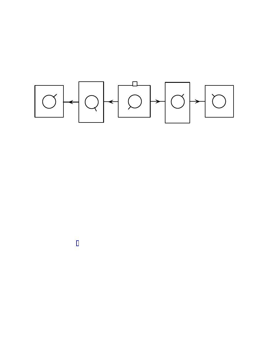
Preparation
Z
A
Z
B
Measurement A
Measurement B
System B
System A
Figure 2: The preparation device here prepares a system in the form of two subsystems which go to the left
and the right.
To discuss the constraints on transformations we need
to consider composite systems.
Fig. 2. shows a
preparation apparatus producing a system made up
of subsystems A and B such that A goes to the
left and B goes to the right.
These subsystems
then impinge on measurement apparatuses after pass-
ing through transformations devices which perform
transformations Z
A
and Z
B
. This set up can be un-
derstood to be a special case of the more generic setup
shown in Fig. 1. (there is no stipulation in the case
of Fig. 1. that the measurement apparatus or any of
the other apparatuses be located only in one place).
Assume the transformation devices are initially set to
leave the subsystems unchanged. From Axiom 4 we
know that there are K
A
K
B
fiducial measurements.
As discussed in Section 5, the space of positive oper-
ators for the composite system is spanned by ˆ
P
A
i
⊗ ˆ
P
B
j
where ˆ
P
A
i
(i = 1 to K
A
) is a fiducial set for A and ˆ
P
B
j
(j = 1 to K
B
) is a fiducial set for B. It is shown in
Appendix 4 that (as we would expect) the projector
ˆ
P
A
i
⊗ ˆ
P
B
j
corresponds (i) to preparing the ith fiducial
state at side A and the jth fiducial state at side B
when the operator is regarded as representing a state,
and (ii) to measuring the joint probability of obtain-
ing a positive outcome at both ends when the ith fidu-
cial measurement is performed at side A and the jth
fiducial measurement is performed at side B when the
operator is regarded as representing a measurement.
Hence, one choice of fiducial measurements is where
we simply perform the ith fiducial measurement on
A and the jth fiducial measurement on B and mea-
sure the joint probability p
ij
. The probabilities p
ij
could be put in the form of a column vector p
AB
.
However, for discussing transformations, it is more
convenient to put them in the form of a K
A
× K
B
matrix, ˜
p
AB
, having ij entry p
ij
. It is easy to con-
vert between these two ways of describing the state.
We could regard both the preparation apparatus and
measurement apparatus B as a preparation appara-
tus preparing states of subsystem A. If we perform
the jth fiducial measurement on system B and take
only those cases where we obtain a positive result for
this measurement preparing the null state otherwise
then the resulting state of system A will be given
by a vector equal to the jth column of ˜
p
AB
(since
these probabilities are equal to the probabilities that
would be obtained for the fiducial measurements on
A with this preparation). Hence, the columns of ˜
p
AB
must transform under Z
A
. Similarly, the rows of ˜
p
AB
24

must transform under Z
B
. Hence, when the transfor-
mation devices in Fig. 2. are active, we have
˜
p
AB
→ Z
A
˜
p
AB
Z
T
B
(97)
If the state is represented by ˜
r
AB
where
˜
p
AB
= D
A
˜
r
AB
D
T
B
(98)
then this equation becomes
˜
r
AB
→ X
A
˜
r
AB
X
T
B
(99)
where
X
A
= D
−1
A
Z
A
D
A
(100)
and similarly for B. It is easy to see that this is the
correct transformation equation in quantum theory
(we have dropped the A and B superscripts).
p
ij
AB
→ tr[ ˆ
P
i
⊗ ˆ
P
j
$
A
⊗ $
B
(ˆ
ρ)]
=
tr[ ˆ
P
i
⊗ ˆ
P
j
$
A
⊗ $
B
(
P
kl
ˆ
P
k
⊗ ˆ
P
l
r
kl
)]
=
P
kl
tr[ ˆ
P
i
⊗ ˆ
P
j
$
A
( ˆ
P
k
)
⊗ $
B
( ˆ
P
l
)]r
kl
=
P
kl
tr[ ˆ
P
i
$
A
( ˆ
P
k
)]r
kl
AB
tr[ ˆ
P
i
$
B
( ˆ
P
l
)]
(101)
which, using (96), gives (97) and (99). The steps
in (101) can be read backwards. Hence, from (97),
we obtain the tensor product structure for describing
composite systems.
We will say that Z
A
is completely positive iff
˜
p
AB
→ Z
A
˜
p
AB
(102)
maps all allowed states of the composite system AB
to states which are also allowed states for any di-
mension N
B
. The only constraint on transforma-
tion matrices Z is that they transform states in S
to states in S. This means that probabilities must
remain bounded by 0 and 1. Hence,
1. Z must not increase the normalization coefficient
of states.
2. Z must be completely positive.
Condition 2 is necessary since any system could al-
ways be a subsystem of some larger system. The
transformations deduced from the axioms are subject
to the equivalent constraints for $ listed in Section 5.
They preserve Hermitivity since the transformation
matrix Z is real (and hence p remains real). They
do not increase the trace (point 1. above). They are
linear and they must be completely positive (point 2.
above). Hence, the most general type of transforma-
tion consistent with the axioms is the most general
transformation of quantum theory. As noted in sec-
tion 5, this gives us unitary evolution and von Neu-
mann projection as special cases.
8.9
The state after a measurement
It is possible that, after a measurement, a quantum
system emerges from the measurement apparatus. In
such cases the measurement apparatus is also behav-
ing as a transformation apparatus. We can think of
the state as emerging into a different channel for each
measurement outcome. Associated with each out-
come, l, of the measurement will be a certain trans-
formation, Z
l
∈ Γ, on the state. The probability of
any given outcome will not, in general, be equal to 1.
Hence, the transformation must reduce the normal-
ization coefficient associated with the state to a value
consistent with the probability of obtaining that out-
come. This condition is
r
I
· Z
l
p = r
l
· p
for all p
∈ S
(103)
Furthermore, we can consider all these channels taken
together. In this case the effective transformation is
given by
P
l
Z
l
. It is necessary that this also belongs
to the allowed set of transformations, Γ, and that it
does not change the normalization coefficient associ-
ated with the state. This second condition can be
written
X
l
Z
l
T
r
I
= r
I
(104)
This is equivalent to constraint
tr
X
l
$(ˆ
ρ) = tr(ˆ
ρ) for all
ˆ
ρ
(105)
Since completely positive operators can be written as
$(ˆ
ρ) =
P
l
ˆ
M
l
ˆ
ρ ˆ
M
†
l
this equation can be shown to be
25

equivalent to
X
l
ˆ
M
†
l
ˆ
M
l
= ˆ
I
(106)
which is the usual quantum constraint on superoper-
ators associated with measurements [14, 15].
The two equations (103,104) which constrain the
possible transformations of the state after measure-
ment apply equally well to classical probability the-
ory. This may suggest a new approach to the mea-
surement problem in quantum theory.
9
Infinite dimensional spaces
There are two types of infinite dimensional space -
countable and continuous dimensional. The count-
able infinite dimensional spaces are accounted for by
these axioms since such systems are characterized by
the property that any finite subspace obeys quantum
theory. It is not so clear what the status of contin-
uous dimensional spaces is. Such spaces can always
be modeled arbitrarily well by a countable infinite di-
mensional Hilbert space. However, there are certain
mathematical subtleties associated with the continu-
ous case which we have not considered here. Never-
theless, it is clear that the classical continuous case
violates the axioms even though there are continuous
paths between states since the continuity axiom (Ax-
iom 5) must also apply to finite subspaces (by Axiom
3) and for these there are no continuous transforma-
tions.
While continuous dimensional spaces play a role in
some applications of quantum theory it is worth ask-
ing whether we expect continuous dimensional spaces
to appear in a truly fundamental physical theory of
nature. Considerations from quantum gravity sug-
gest that space is not continuous at the planck scale
and that the amount of information inside any finite
volume is finite implying that the number of distin-
guishable states is countable. Given the mathemat-
ical difficulties that appear with continuous dimen-
sional Hilbert spaces it is also natural to ask what
our motivation for considering such spaces was in the
first place. Consider a classical particle which can
move along a straight line. If where were not a con-
tinuous infinity of distinguishable positions for the
particle then the only way the particle could move
would be to jump from one position to the next. It is
because we do not like such discontinuities in physics
that we imagine that there is a continuous infinity of
distinct positions along the line. However, in quan-
tum theory it is no longer the case that the particle
would need to jump and hence the main motivation
for considering the continuous dimensional case no
longer pertains.
If we do, nevertheless, consider continuous dimen-
sional spaces then there is an interesting respect in
which the quantum case is superior to the classi-
cal case. Consider again a particle which can move
along a straight line. Every point on the line repre-
sents a distinguishable state for the particle. Take
three points A, B, and C along this line where B is
between A and C. In classical theory, if the parti-
cle is to move continuously through the state space
from A to C it must pass through point B. How-
ever, to move continuously from A to B it need not
pass through C. Hence, the pairs AB and AC are
on an unequal footing. In quantum theory a particle
can pass directly from the point A to the point C
without going through the points in between along
a continuous trajectory in the state space simply by
going along the Bloch sphere corresponding to this
two-dimensional subspace (such transformations do
not occur in practise since Hamiltonians contain only
local terms). Hence, the pairs AB and AC are on an
equal footing. We can regard statements like “the
particle is at point B” as logical propositions. It is
a very desirable property that pairs of propositions
should be on an equal footing. Thus, in this respect,
quantum theory is superior.
On the other hand, even in the quantum case, con-
tinuous dimensional spaces appear to have a topo-
logical relationship between infinitesimally displaced
distinguishable states which is different to the topo-
logical relationship between finitely displaced distin-
guishable states. This is hard to reconcile with the
notion that any pair of distinguishable states are on
an equal footing and may be further support for the
case against giving continuous dimensional spaces a
role in any fundamental theory of nature.
26

10
Discussion
We have shown that quantum theory follows from
five very natural axioms. If Axiom 5 (or even just
the word “continuous” in Axiom 5) is dropped we
obtain classical probability theory instead. It is clas-
sical probability theory that must have ‘jumps’. If
a 19th century ancestor of Schroedinger had com-
plained about “dammed classical jumps” then he
might have attempted to derive a continuous the-
ory of probability and arrived at quantum theory.
Quantum theory is, in some respects, both superior
to and more natural than classical probability theory
(and therefore classical theories in general) since it
can describe evolution for finite systems in a contin-
uous way. Since nature is quantum, not classical, it
is to be expected that quantum theory is ultimately
the more reasonable theory.
There are many reasons to look for better ax-
iomatic formulations of quantum theory.
• Aesthetics. A theory based on reasonable axioms
is more appealing.
• A set of reasonable axioms provides us with a
deeper conceptual understanding of a theory and
is therefore more likely to suggest ways in which
we could extend the domain of the theory or
modify the axioms in the hope of going beyond
quantum theory (for example, to develop quan-
tum gravity).
• This approach puts a different slant on the in-
terpretation of quantum theory (see discussion
below).
• Since the formulation of quantum theory here
is closer to classical probability theory than the
standard formulation, this may motivate new ap-
plications and new treatments of the theory of
quantum information.
There are various ways in which this work has a
bearing on interpretational matters. First, if we re-
ally believe these axioms to be reasonable then they
would also apply to hidden variables and it would fol-
low that the hidden variable substructure must look
like quantum theory. We could not then use hidden
variables to solve the measurement problem (since
this relies on being able to give the hidden variables
a classical probability interpretation). Second, we
see here how successful a purely instrumentalist ap-
proach is in obtaining the structure of quantum the-
ory. Whilst this need not contradict beliefs held by
the realist since he would anyway expect quantum
theory to be consistent with instrumentalist argu-
mentation, it does require some explanation. And,
third, we obtain that the most general evolution is
that of a superoperator. This is capable of taking
pure states to mixed states. Hence, collapse interpre-
tations of quantum theory could be incorporated into
this structure.
Acknowledgements
I am very grateful to Chris Fuchs for discussions
that motivated this work and to Jeremy Butterfield,
Philip Pearle, Terry Rudolph, and Jos Uffink for com-
ments. This work is funded by a Royal Society Uni-
versity Research Fellowship.
References
[1] G. Birkhoff and J. von Neumann, Ann. Math.
37, 743 (1936).
[2] G. W. Mackey, The mathematical foundations of
quantum mechanics (W. A. Benjamin Inc, New
York, 1963).
[3] J. M. Jaunch and C. Piron, Helv. Phys. Acta 36,
837 (1963); C. Piron, Helv. Phys. Acta 37, 439
(1964).
[4] G. Ludwig, Commun. Math. Phys. 9, 1 (1968),
G. Ludwig, Foundations of quantum mechanics
volumes I and II (Springer-Verlag, New York,
1983 and 1985).
[5] B. Mielnik, Commun. Math. Phys. 9, 55 (1968).
[6] A. Lande, Am. J. Phys. 42, 459 (1974).
[7] D. I. Fivel, Phys. Rev. A 50 2108 (1994).
27

[8] L. Accardi, Il Nuovo Cimento 110B, 685 (1995).
[9] N. P. Landsman, Int. J. of Theoretical Phys.
37, 343 (1998) and Mathematical topics between
classical and quantum mechanics (Springer, New
York, 1998).
[10] B. Coecke, D. Moore, A. Wilce, Current re-
search in operational quantum logic: algebras,
categories, languages (Fundamental theories of
physics series, Kluwer Academic Publishers,
2000), also available on quant-ph/0008019.
[11] A. M. Gleason, Annals of Math 6, 885 (1957).
[12] S. Kochen and E.P. Specher, J. Math and Mech.
17, 59 (1967).
[13] I. Pitowsky, Lecture notes in physics 321
(Springer-Verlag, Berlin-Heildelburg 1989).
[14] K. Kraus,
States, effects, and operations:
Fundamental
notions
of
quantum
theory
(Springer-Verlag,
Berlin,
1983);
B. Schu-
macher, quant-ph/9604023 (appendix A); J.
Preskill Lecture notes for physics 229: quantum
information and computation,
available at
(see chapter 3).
[15] M. A. Nielsen and I. L. Chuang, Quantum infor-
mation and quantum information, (Cambridge
University Press, 2000).
[16] R. Schack, private communication.
[17] D. Deutsch, private communication.
[18] W. K. Wootters, Local accessibility of quantum
states, in Complexity, entropy and the physics
of information edited by W. H. Zurek (Addison-
Wesley, 1990) and W. K. Wootters, Found. Phys
16, 319 (1986).
[19] S. Weigert, Phys. Rev. Lett. 84, 802 (2000).
[20] It has been noted by C. Caves, C. Fuchs and
R. Schack in quant-ph/0104088 that difficulties
in formulating a De Finetti theorem for quater-
nionic quantum theory stem from the fact that
K
6= K
A
K
B
.
[21] H. Boerner, Representations of groups (North-
Holland publishing company, Amsterdam 1963).
Appendix 1
We will prove that the property
f(λp
A
+ (1
− λ)p
B
) = λf(p
A
) + (1
− λ)f(p
B
),
(107)
where λ
≥ 0, implies that
f(p) =
X
α
a
α
f(p
α
)
(108)
where
p =
X
α
a
α
p
α
(109)
if
p
α
, p
∈ S for all α
for all a
α
where S is the set of allowed p. First note
that putting p
A
= 0 gives
f(λp) = λf(p)
(110)
for 0
≤ λ ≤ 1. We can write γ = 1/λ and p
00
= p/λ.
Then we obtain
f(γp
00
) = γf(p
00
)
(111)
where 1
≤ γ. Hence,
f(νp) = νf(p)
(112)
if ν
≥ 0. This only follows from (107) if p, νp ∈ S.
However, if this is not the case, then the equation
does not correspond to any physical situation. Hence,
we are free to impose that (112) is true for all p.
In those cases where p, νp
∈ S is not satisfied the
equation has no physical significance anyway.
Let f
I
pertain to that measurement that simply
checks to see that a non-null result has been recorded
(we call this the identity measurement).
We will
28

write f
I
(p) = µ. We define the normalized state
˜
p by µ˜
p = p such that f
I
(˜
p) = 1 (using (112)).
We can normalize each of the states in (109) such
that
µ˜
p =
X
α
a
α
µ
α
˜
p
α
(113)
We are free to choose the fiducial measurement cor-
responding to the first component of the state vector
p to be the identity measurement. Hence, reading off
the first component from (113) we obtain
µ =
X
α
a
α
µ
α
(114)
Let α
∈ A
±
if a
α
is
±ve and define
ν = µ +
X
α
∈A
−
|a
α
|µ
α
=
X
α
∈A
+
a
α
µ
α
(115)
We can rearrange (113)
µ
ν
˜
p +
X
α
∈A
−
|a
α
|µ
α
ν
˜
p
α
=
X
α
∈A
+
a
α
µ
α
ν
˜
p
α
(116)
Each coefficient is positive and the coefficients on
each side add to 1. Hence we can apply (107)
µ
ν
f(˜
p) +
X
α
∈A
−
|a
α
|µ
α
ν
f(˜
p
α
) =
X
α
∈A
+
a
α
µ
α
ν
f(˜
p
α
)
(117)
Rearranging this using (112) gives (108) as required.
We see that (108) holds whenever the arguments
of f in each term correspond to physical states. If
these arguments do not all correspond to physical
states then the equation does not correspond to any
physical situation. For mathematical simplicity we
will impose that (108) still holds in such cases.
Appendix 2
In this appendix we show that any strictly in-
creasing function having the completely multiplica-
tive property
K(mn) = K(m)K(n),
(118)
where n takes only positive integer values, is of the
form K(n) = n
α
. First put m = n = 1 into (118).
We obtain that K(1) = 0, 1.
Put m = 1 into
(118). If K(1) = 0 then K(n) = 0 for all n. But
this is not strictly increasing. Hence we must have
K(1) = 1. The argument n can be factorized into
primes: n = p
k
1
1
p
k
2
2
. . . where p
i
is the ith prime and
the k
i
’s are integers. It follows from the completely
multiplicative property that
K(n) =
Y
i
K
k
i
(p
i
)
(119)
Hence, the function K(n) is completely determined
by its values at the primes. Now consider two primes
p and q. Define α by
K(p) = p
α
(120)
Note that K(p) > 1 since K(n) is a strictly increasing
function and hence α > 0. Define a by
K(q) = aq
α
(121)
Introduce the integer t which we will allow to take
any positive value. Then define s by
p
s
> q
t
> p
s
−1
(122)
From the fact that K(n) is strictly increasing we have
K(p
s
) > K(q
t
) > K(p
s
−1
)
(123)
Hence,
p
αs
> a
t
q
αt
> p
α(s
−1)
(124)
Define
es by
p
e
s
= q
t
(125)
Comparing with (122) we have
es + 1 > s > es > s − 1 > es − 1
(126)
Hence, (124) gives
p
α(
e
s+1)
> a
t
q
αt
> p
α(
e
s
−1)
(127)
29

(we have used the fact that α > 0). Using (125) we
obtain
p
α
> a
t
> p
−α
(128)
This must be true for all t. However, a
t
can only
be bounded from above and below if a = 1. Hence,
K(q) = q
α
. This applies to any pair of primes, p and
q, and hence K(n) = n
α
.
Appendix 3
In this appendix we will prove a number of related
important results some of which are used in the main
part of the paper.
The set of reversible transformations is represented
by the set, Γ
reversible
, of invertible matrices Z in Γ
whose inverses are also in Γ. These clearly form a
representation of a group. In fact, since, by Axiom 5,
this group is continuous and the vectors p generated
by the action of the group remain bounded, Γ
reversible
is a representation of a compact Lie group. It can
be sown that all real representations of a compact
Lie group are equivalent (under a basis change) to a
real orthogonal representation [21]. Let us perform
such a basis change. Under this basis change assume
that Z
∈ Γ is transformed to Y ∈ Ω and p
S
∈ S is
transformed to q
∈ Q. The formula p
meas
= r
· p
becomes
p
meas
= s
· q
(129)
where s now represents the measurement (and is ob-
tainable from r by a basis change). If a transforma-
tion device is present then we have
p
meas
= s
T
Y q
(130)
We can regard Y as transforming the state or, alter-
natively, we can regard it as part of the measurement
apparatus. In this case we have s
→ Y
T
s. If we
now restrict our attention to reversible transforma-
tions then Y
∈ Ω
reversible
. But this is an orthogonal
representation and hence Y
T
∈ Ω
reversible
. Therefore,
with this representation, both states q and measure-
ments s are acted on by elements of Ω
reversible
.
A3.1
In this Appendix section we will prove that
Z
T
W
r
I
W
= r
I
W
for all Z
W
∈ Γ
reversible
W
(131)
where r
I
W
is the identity measurement for the sub-
space W and Γ
reversible
W
is the set of reversible trans-
formations which map states in the subspace W to
states in W – such transformations must exist by Ax-
iom 3. We can work in the basis for which the trans-
formations are orthogonal introduced above. Then
we wish to prove
Y
T
W
s
I
W
= s
I
W
for all Y
W
∈ Ω
reversible
W
(132)
Working in this basis we can write any state in the
subspace W as
q = as
I
W
+ x
(133)
where x is orthogonal to s
I
. The normalization of this
state is fixed by a. Let K
W
be the number of degrees
of freedom associated with the subspace W . Once
the normalization coefficient has been fixed there are
K
W
− 1 degrees of freedom left corresponding to the
K
W
− 1 dimensions of the vector space orthogonal to
s
I
W
for states in W which is spanned by possible x.
There must be at least one direction in this vector
space for which both x and γx, where γ
6= 1, are per-
missible vectors (corresponding to allowed states). To
see this assume the contrary. Thus assume that for
each direction x/
|x| there is only one allowed length
of vector. Such a constraint would remove one degree
of freedom leaving K
W
− 2 degrees of freedom which
contradicts our starting point that there are K
W
− 1
degrees of freedom associated with states with a par-
ticular normalization coefficient. Consider such an x
for which γx is also permissible. Now
s
I
W
· Y
W
q = s
I
W
· q
(134)
since the reversible transformation Y
W
does not
change the normalization coefficient of the state and
q is in W both before and after the transformation.
Using (133) this becomes
as
I
W
· Y
W
s
I
W
+ s
I
W
· Y
W
x = as
I
W
· s
I
W
(135)
30

This equation must also apply when x is replaced by
γx.
as
I
W
· Y
W
s
I
W
+ γs
I
W
· Y
W
x = as
I
W
· s
I
W
(136)
Subtracting these two equations tells us that the sec-
ond term on the LHS vanishes. Hence
s
I
W
· Y
W
s
I
W
= s
I
W
· s
I
W
(137)
Now, the transformation Y
W
is orthogonal and hence
length preserving and thus (132) follows.
It follows that
Y
T
s
I
= s
I
for all Y
∈ Ω
reversible
(138)
where s
I
is the identity measurement in this new basis
(written as r
I
in the usual basis). This property is
to be expected since reversible transformations leave
the normalization coefficient of a state unchanged.
A3.2
It is clearly the case that
Z
W
p
∈ W if p ∈ W and Z
W
∈ Γ
reversible
W
(139)
It is also the case that
Z
W
p
∈ W if p ∈ W and Z
W
∈ Γ
reversible
W
(140)
where W is the complement subspace of W . This
follows immediately since p
∈ W iff r
I
W
· p = 0. But
if this is true then, since Z
T
W
r
I
W
= r
I
W
, it is also true
that r
I
W
· Z
W
p = 0. Hence, Z
W
p
∈ W .
A3.3
We will now prove that we can choose Z
W
such
that Z
W
p
n
= p
n
for n
∈ W . Define W
0
(m) to be
the set containing all the elements of W plus the first
m elements of W . Consider only states constrained to
the subspace W
0
(1) and consider the set Γ
reversible
W
0
(1)
of
reversible transformations which map states in W
0
(1)
back into W
0
(1). The subspace W is a subspace of
W
0
(1). Hence, by Axiom 3, there must exist a subset
of Γ
reversible
W
0
(1)
which map states in W back into W . By
the result in A3.2 these transformations must leave
the basis state p
m
1
unchanged (where m
1
is the first
entry of W ) since this is the only normalized state in
W
0
(1) and the complement of W . We can now run
the same argument taking W
0
(2) to be our system
and so on. In this way we establish that we can find a
transformations Z
W
which have the desired property.
A3.4
In this appendix subsection we show that one pos-
sible choice of fiducial measurements are those iden-
tified in Section 8.2. Consider the set Γ
reversible
mn
of re-
versible transformations that transform states in the
subspace W
mn
to states in the same subspace (where
W
mn
is the subspace associated with the mth and
the nth basis vectors). It follows from the property
established in A3.2 that
r
T
n
Z
mn
p = 0
if
p
∈ W
mn
(141)
We can regard the transformation device as part of
the measurement apparatus (rather than regarding it
as acting on the state). In this case we have
r
n
→ Z
T
mn
r
n
(142)
We can choose two particular transformations Z
mnx
and Z
mny
to provide us with the two extra needed
fiducial measurements, r
mnx
and r
mny
respectively,
for each two-dimensional subspace. The vectors r
m
,
r
n
, r
mnx
, and r
mny
must be linearly independent.
It follows from the fact that, for this subspace, the
group of transformations is equivalent, under a basis
change, to the full group of orthogonal rotations in
three dimensions that we can choose Z
mnx
and Z
mny
such that this is the case. From (141) we have
r
mnx
· p = 0 if p ∈ W
mn
(143)
and similarly for r
mny
.
We will now prove that the N
2
vectors chosen in
this way are linearly independent. We can do this by
showing that each measurement yields information
about the state that none of the others do. First,
the vectors r
n
are linearly independent of each other
31

since there exists a vector (namely p
m
) having non-
zero overlap with any given r
m
which has zero over-
lap with all the other r
n
. Now we add two fidu-
cial vectors, r
mnx
and r
mny
, to each two-dimensional
subspace W
mn
that are, by construction, linearly in-
dependent of the basis vectors already in that sub-
space. Since the fiducial measurements pertaining to
one such two-dimensional subspace yield no informa-
tion about states in any other non-overlapping two-
dimensional subspace (because of (143))they must be
linearly independent of the fiducial measurements in
those non-overlapping subspaces. What about over-
lapping two-dimensional subspaces? Consider per-
forming the measurement r
mnx
on p in W
mn
0
where
n
0
6= n. Since p is in W
mn
0
it follows from Axiom
3 that the measurement r
mnx
must be equivalent to
some measurement in this subspace (though only for
states in this subspace). Now, if the state is actually
the basis state p
n
0
then zero probability would be
recorded. This means that the measurement r
mnx
,
when regarded as a measurement on W
mn
0
is actu-
ally equivalent to a measurement just on the one-
dimensional subspace W
m
. Hence, r
mnx
does not
yield any information about states in the subspace
W
mn
0
that is not given by r
m
and therefore the mea-
surements r
mn
0
x
and r
mn
0
y
are linearly independent
of it. Hence, the N
2
fiducial measurements are all
necessary to determine the state and are therefore
linearly independent.
A3.5
In this appendix subsection we show that the map
between a pure state and that pure measurement
identifying it is linear and invertible (recall that pure
measurements are defined to be those measurements
which can be obtained by acting on the basis mea-
surement r
1
with a reversible transformation). Using
the basis for which reversible transformations are or-
thogonal (see introduction to this appendix) we can
put
q = as
I
+ u
(144)
for the state, and
s = bs
I
+ v
(145)
for the measurement where u and v are orthogonal to
s
I
. Since Y
T
s
I
= s
I
and since the group of reversible
transformations, Ω
reversible
, is orthogonal it follows
that Y s
I
= s
I
. Hence, transformations only effect
the components of q and s orthogonal to s
I
. Using
p
meas
= r
· p = s · q we obtain
p
meas
= k + v
· u
(146)
where k = abs
I
· s
I
.
Now assume that the pure measurement repre-
sented by s identifies the pure state represented by
q. Then k + u
· v = 1. This probability cannot be
increased by any transformation device. Hence,
v
T
Y u
≤ v
T
u for all Y
∈ Ω
reversible
(147)
Since the orthogonal transformation Y is length pre-
serving it would appear that the only way to satisfy
this condition is if v is parallel to u. This is indeed
the case and is proven at the end of this appendix sub-
section. Hence, we can say that the state q = as
I
+u
is identified by the measurement s = bs
I
+ cu. Now
apply this result to the basis state q
1
(this corre-
sponds to p
1
) and the basis measurement s
1
(this
corresponds to r
1
). Let C be the linear map that
performs scalar multiplication by a factor µ in the s
I
direction and by a factor ν in the subspace orthogo-
nal to s
I
. We can apply C to q and C
−1
to s such
that s
1
= q
1
= αs
I
+βu
1
by appropriate choice of the
factors µ and ν. The maps C and C
−1
commute with
the orthogonal transformations Ω
reversible
. Hence, in
general, the pure state q = αs
I
+ Y βu
1
is identified
by the pure measurement s = αs
I
+ Y βu
1
(i.e. rep-
resented by the same vector) as Y Y
T
= I. Since the
basis change and the maps C and C
−1
are all lin-
ear and invertible it follows that the map from pure
states to the pure measurements identifying them is
linear and invertible.
As promised, we will now prove that v is parallel
to u when a pure measurement s identifies a pure
state q. First consider the basis measurement s
1
and
the basis state q
1
it identifies. Let V
mn
be the vector
space spanned by the fiducial measurement vectors
s
m
, s
n
, s
mnx
and s
mny
associated with the mn sub-
space. It follows from A3.4 that these vector spaces
span the full N
2
dimensional vector space. The state
32

q
1
can have no projection into the vector space V
mn
if
m, n
6= 1 (since s·q
1
= 0 for s associated with the mn
subspace). Let e
V be the vector space spanned by the
vector spaces V
1n
for n = 1 to N . It follows from the
fact that q
1
has no projection into V
mn
for m, n
6= 1
that q
1
is in e
V . Now the vector s
I
=
P
n
s
n
is clearly
in e
V . Let e
V
0
be the vector space in e
V orthogonal to
s
I
. We can write q
1
= as
I
+ u
1
where u
1
is in the
vector space e
V
0
. Similarly, we can write s
1
= bs
I
+v
1
.
Define V
0
1n
as the vector space spanned by the fiducial
measurement vectors v
1
, v
n
, v
1nx
, and v
1ny
associ-
ated with the subspace 1n. The vector spaces V
0
1n
for
n = 1 to N span e
V
0
. Consider orthogonal transfor-
mations Y
1n
which leave states in the 1n subspace.
They will also transform measurements pertaining to
the 1n subspace to measurements still pertaining to
this subspace (and thus still in V
0
1n
). Since v
1
and
Y
T
1n
v
1
are both in V
0
1n
we can write (147) as
v
T
1
Y
1n
u
1n
1
≤ v
T
1
u
1n
1
(148)
where u
1n
1
is the component of u
1
in V
0
1n
. The vec-
tor space V
0
1n
is three dimensional and the action of
the group of orthogonal transformations in the 1n
subspace on u
1
is to sweep out a sphere (since these
transformations are length preserving). Hence, con-
dition (148) can only be satisfied for all rotations Y
1n
if u
1n
1
is parallel to v
1
. The vector spaces V
0
1n
span
all of e
V
0
and hence u
1
has no component which is
perpendicular to v
1
. This means that v
1
is parallel
to u
1
. We complete the proof by noting that a gen-
eral pure measurement can be written v = Y v
1
and
identifies the pure state u = Y u
1
.
A3.6
It is easy to prove that D = D
T
. We chose a
set of pure fiducial states and we chose the fiducial
measurements to be the set of pure measurements
that identify these states. Hence, if we represent the
fiducial states by a set of vectors q
l
then, as proven
in A3.5, we can represent the fiducial measurements
by the the same vectors s
k
= q
k
. The matrix element
D
kl
is equal to the probability when the kth fiducial
measurement is performed on the lth fiducial state.
This is equal to q
k
· q
l
and hence D = D
T
.
A3.7
Now we will show that the basis measurements r
n
are all pure and, therefore, that all the fiducial mea-
surements of A3.4 are pure. Consider first the case
where N = 2. Then K = 4. The normalized states
(and hence pure states) live in a three dimensional
space (since we can eliminate one variable by nor-
malization). Hence, orthogonal transformations can
be regarded as rotations about an axis. We can write
the basis states as
q
1
= αs
I
+ βu
1
(149)
q
2
= αs
I
− βu
1
(150)
This follows since there exists a continuous orthogo-
nal transformation which takes q
1
to q
2
. This can
be regarded as a rotation around a great circle. The
orthogonal state q
2
must correspond to the opposite
point on this circle where u =
−u
1
since this is the
point at which s
1
· q stops decreasing and starts in-
creasing again. Now, we have already that
s
1
= αs
I
+ βu
1
(151)
We have not yet proven that s
2
(corresponding to r
2
)
is pure. However, we know that s
1
+ s
2
= s
I
so we
can write
s
2
= α
0
s
I
− βu
1
(152)
with α + α
0
= 1. It then follows from s
1
· q
2
=
s
2
·q
1
= 0 that α = α
0
= 1/2. Hence, s
2
is pure. This
proof can be applied to the general N case by con-
sidering only a two dimensional subspace. It follows
from Axiom 3 that there must exist a set of invert-
ible transformations which transform states in the 1n
subspace to states in the same subspace. As shown in
A3.1, these leave s
I
W1n
invariant (this is the identity
measurement vector for the 1n subspace). Hence, we
can replace s
I
by s
I
W1n
throughout the above proof if
we are only considering transformations in this sub-
space. It follows that we can transform s
1
to s
n
and
hence the basis measurements are all pure.
Hence we can transform s
1
to any s
mnx
by first
transforming by a reversible transformation to s
n
and
33

then applying the reversible transformation of A3.4
to obtain s
mnx
. Similar remarks apply to s
mny
.
Appendix 4
In this appendix we will show that the projector
ˆ
P
A
i
⊗ ˆ
P
B
j
can correspond to the measurement of the
joint probability of obtaining a positive outcome for
fiducial measurements i at A and j at B, and to the
state when the ith fiducial state is prepared at A and
the jth fiducial state is prepared at B. First, note
that we can prepare N
A
N
B
distinguishable states for
the composite system by preparing basis state m at
A and basis state n at B. Since the composite sys-
tem has N = N
A
N
B
this represents a complete set
of basis states. Further, since K(1) = 1 all basis
states must be pure (as noted at the end of Section
8.1). Hence, we can choose these basis states to cor-
respond to the basis states of our Hilbert space
|mni
or, equivalently,
|mi ⊗ |ni. As operators these ba-
sis states are ˆ
P
A
m
⊗ ˆ
P
B
n
where m (n) only runs over
the first N
A
(N
B
) values (the remaining values cor-
responding to the other fiducial projectors).
Now consider the N
B
dimensional subspace with
basis states
|1i ⊗ |ni (n = 1 to N
B
). This subspace
corresponds to the case where system A is prepared
in basis state 1 and system B is prepared in any state.
A full set of fiducial projectors can be formed for this
subspace. These will take the form ˆ
P
A
1
⊗ ˆ
P
B
l
where
l = 1 to K
B
(i.e. runs over the all values, not just
the basis labels). We can do the same for the case
where basis state 2 is prepared at A. Then we have
the fiducial projectors ˆ
P
A
2
⊗ ˆ
P
B
l
for the subspace 2n
(n = 1 to N
B
). Indeed, we can do this for the gen-
eral case in which the basis state m is prepared at A.
Now consider the pure state ˆ
P
A
1
⊗ ˆ
Q
B
where ˆ
Q
B
is
some arbitrary projector at B. This state is in the 1n
(n = 1 to N
B
) subspace and we can perform the fidu-
cial measurements ˆ
P
A
1
⊗ ˆ
P
B
l
in this subspace to fully
characterize this state. The probabilities obtained in
making these fiducial measurements will be the same
as if we prepared the state ˆ
P
A
2
⊗ ˆ
Q
B
and made the
fiducial measurements ˆ
P
A
2
⊗ ˆ
P
B
l
and hence this corre-
sponds to the same preparation at B. Hence, in gen-
eral the projector ˆ
P
A
m
⊗ ˆ
Q
B
corresponds to preparing
the basis state ˆ
P
m
at A and the general pure state
ˆ
Q
B
at B. Now consider the subspace spanned by
the projectors ˆ
P
A
m
⊗ ˆ
Q
B
(m = 1 to N
A
) in which we
prepare ˆ
Q
B
at B. A fiducial set for this subspace is
ˆ
P
A
k
⊗ ˆ
Q
B
where k = 1 to K
A
. If these fiducial mea-
surements are made on a state ˆ
R
A
⊗ ˆ
Q
B
where ˆ
R
A
is
a projector at A then we would get the same results
as if the fiducial measurements ˆ
P
A
k
⊗ ˆ
Q
0
B
were made
on the state ˆ
R
A
⊗ ˆ
Q
0
B
. Hence, in both cases the
preparation at A is the same. Thus, the pure state
ˆ
R
A
⊗ ˆ
Q
B
corresponds to the case where a particu-
lar pure state ˆ
R
A
is is prepared at A and the pure
state ˆ
Q
B
is prepared at B. An analogous argument
to that above can be used to show that, regarded as
a measurement, the projector ˆ
R
A
⊗ ˆ
Q
B
corresponds
to measuring the joint probability with setting ˆ
R
A
at end A and setting ˆ
Q
B
at end B. Applied to the
fiducial projectors, ˆ
P
A
k
⊗ ˆ
P
B
l
, this proves our result.
34
Wyszukiwarka
Podobne podstrony:
Hardy, Lyndon Magics 01 The Master of Five Magics
George Starbuck The Works, Poems Selected from Five Decades
Attribution theory from a neuropsychological perspective
General Relativity Theory, Quantum Theory of Black Holes and Quantum Cosmology
Feynman s Path Integral in Quantum Theory
Donald M J Quantum theory and the brain
Laudal O A Geometry of time spaces Non commutative algebraic geometry, applied to quantum theory (WS
Freitag Several complex variables local theory (lecture notes, web draft, 2001)(74s) MCc
Finn From Counting to Calculus (2001) [sharethefiles com]
Five Reasons To Get Cancer John Tarrant (Zen, Buddhism, Koan)
Five reasons you Can’t ignore Gamification
Pratt S Quantum mechanics problem sets (lecture notes, 2001)(35s) PQmtb
Hardy ?r from the Madding Crowd
Guerin Anarchism From Theory to Practice (1970)
Modanese Inertial Mass and Vacuum Fluctuations in Quantum Field Theory (2003)
Escobedo M , Mischler S , Valle M A Homogeneous Boltzmann equation in quantum relativistic kinetic t
Seahra S Path integrals in quantum field theory (web draft, 2002)(36s) PQft
Alvarez Gaume L , Introductory Lectures on Quantum Field Theory
więcej podobnych podstron