Worm Anatomy and Model

Worm Anatomy and Model

Dan Ellis

The MITRE Corporation

7515 N. Colshire Dr.
McLean, VA 22102

ellisd@mitre.org

ABSTRACT

We present a general framework for reasoning about network worms
and analyzing the potency of worms within a specific network. First,
we present a discussion of the life cycle of a worm based on a
survey of contemporary worms. We build on that life cycle by
developing a relational model that associates worm parameters,
attributes of the environment, and the subsequent potency of the
worm. We then provide a worm analytic framework that captures
the generalized mechanical process a worm goes through while
moving through a specific environment and its state as it does so.
The key contribution of this work is a worm analytic framework.
This framework can be used to evaluate worm potency and develop
and validate defensive countermeasures and postures in both static
and dynamic worm conflict. This framework will be implemented in
a modeling and simulation language in order to evaluate the potency
of specific worms within an environment.

Categories and Subject Descriptors

K.6.5 [Security and Protection]: Invasive Software; C.2.0
[Computer-Communication Networks]: Security and Protection;
H.1 [Models and Principles]: Miscellaneous; C.4 [Performance of
Systems]: Measurement techniques.

General Terms:

Security

Keywords:

Worm, Network Security, Network Modeling,

Turing Machine

1. INTRODUCTION

The last few years have demonstrated that worms are a serious and
growing threat. Intrusion detection systems (IDS) and the
procedures supporting intrusion detection and incident response do
not currently scale to deal with the worm threat. Worm conflict
across the Internet can be measured in minutes, while worm conflict
within an enterprise may be measured in seconds. In order to defend
against the worm threat, technology developers and researchers must
have a better understanding of the threat, common vocabulary for
reasoning about the worm threat, and an operational understanding
of how worms work. Further, having the means whereby developers
and system defenders can evaluate worm conflict—both the
offensive and defensive tactics and postures—will enable developers
to identify requirements for defensive countermeasures and postures
as well as evaluate those defenses before developing a prototype. It

will likewise give system defenders a better appreciation of the
strategic dimensions they have direct control over in worm conflict.
We present a worm analytic framework to help developers better
tackle the worm threat. Although some may argue the point that
providing a framework for evaluating worm potency aids the
attackers, which it certainly does, we assert that those responsible
for developing defenses cannot possibly do so without
understanding the threat. Further, by analyzing the worm algorithm
and the relationship between worm parameters, the environment,
and worm potency, developers can better identify defenses that will
be effective at countering the worm threat.
This paper is organized as follows. The remainder of Section 1
covers the related work. Section 2 presents a definition of a worm
and a description of its life cycle. This section focuses on describing
the algorithm that worms use to move across a network. We site
historical examples to illustrate the principles throughout. Section 3
presents a relational worm model. The potency of a worm is
dependent on the parameters of the worm and the environment in
which it operates. The relational worm model is a mathematical
articulation of the relationship between the parameters of the worm,
the current state of the environment (including topology and which
hosts are currently infected), and the subsequent state of the
environment. The Worm Coverage Transitive Closure (WCTC) is a
calculation of the final infection set of a worm given an initial state
of the environment and a parameterized worm. WCTC provides a
mechanism for evaluating the final state of a network given a worm
attack in an environment that lacks defenses that can respond within
the time scale of the worm attack. Section 4 presents a mechanical
worm model that augments the relational model to account for time
considerations. A generalized worm algorithm is presented that
captures the life cycle of a worm and serves as a reference for the
development of a Turing Machine model of worm state. The model
can be deterministic or stochastic and allows for discreet reasoning
about worm conflict. This contribution enables the development of
requirements for defensive tactics, strategies, and postures, as well
as validate the impact of implementations in specific worm conflict
scenarios.
Section 5 presents representations of some contemporary worms.
Section 6 presents our conclusions and future work.

1.1 Related Work

Fred Cohen was the first to propose a mathematical definition for
viruses [2] and, later, worms [3]. The English definition of a virus is
roughly equivalent to “a program that can ‘infect’ other programs by
modifying them to include a possibly evolved, copy of itself” [2].
Using the definition, Cohen proves the point that detecting a virus,
and subsequently, a worm [3], when data and code are
interchangeable is undecidable. For the purpose of this paper, we
characterize viruses and worms as being subsets of a more general
class of mobile logic. Viruses are the subset of logics contained in
files that propagate to other files. Worms are the subset of logics that

Permission to make digital or hard copies of all or part of this work for
personal or classroom use is granted without fee provided that copies are
not made or distributed for profit or commercial advantage and that copies
bear this notice and the full citation on the first page. To copy otherwise, or
republish, to post on servers or to redistribute to lists, requires prior
specific permission and/or a fee.
WORM’03, October 27, 2003, Washington, DC, USA.
Copyright 2003 ACM 1-58113-785-0/03/0010...$5.00.

are embodied in processes that can autonomously cause a like
process to execute on remote hosts. Notice that neither subset
perfectly describes what are known as email-borne viruses. In this
paper we focus on worms, although the principles may be general
enough to help reason about other subclasses of mobile logic.
Staniford-Chen, et al [4], developed a graph-based policy and
monitoring capability to detect coordinated behaviors across
networks. The design included policies whose intention it is to
detect worm traffic. The work presented in this paper could be used
to further refine the requirements for such technology. As worm
conflict is extremely time-sensitive, there may be requirements
tradeoffs between performance, sensitivity, and accuracy.
Much work has been performed in analyzing attack graphs and
representing information systems and their vulnerabilities. The
previous work focuses on different characteristics whether they be
operational [5], or software or systems vulnerabilities [6, 7, 8],
which is a superset of the vulnerabilities a worm might exploit. This
work models vulnerabilities and exploits in a way that is a proper
subset of the vulnerabilities of the previous work. Where the
previous work focuses on any arbitrary threat, this work is focused
on a specific threat that requires more specific attention.
Epidemiological studies of viral spread have been provided by [8,
9], which characterize viruses by their birth rates and death rates
where machines interact only locally or by sharing disks. Research
on worm propagation and spread rates is covered at an
epidemiological scale for hypothetical [11] and historical worms
[12]. The work referenced speaks to the impact worms can have on
the Internet. However, they do not capture the mechanics that are
the source of the potency nor do they provide guidance for
developing defenses for an enterprise.
Wang, et al [13], have developed a simulation model that diverges
from the analytical models with the intention of getting a more
refined appreciation for the effects of targeting choices by a worm
and the topology of the target environment. The authors assert that
analytical models are too course grained and abstract away details
that are critical to understanding how worms propagate and
identifying defensive postures and countermeasures. We agree with
the assertion and seek to further the argument by presenting a more
complete model of worms and the environments with that purpose
in mind. They used a simulation model to evaluate the effects of
randomized and targeted immunization of hosts against two specific
worms in two types of environments. To do so they model the worm
(its targeting strategy) and the environment (a description of either a
hierarchical or clustered topology with hosts that are either
susceptible, infected, or immune). The worm targeting strategy they
employ is based on random selection. They differentiate between
two worms that use this strategy: worms that select only one target
host at a time, and worms that infect multiple nodes that are
connected to the infected node at a time. While the model they use is
more explicit than that used in analytical models, it is not explained
in sufficient detail to provide a common simulation framework.
Therefore it is difficult for other researchers to leverage the same
model to evaluate differing approaches. Further, while they identify
key components—the environment and the algorithm used by the
worm—the details of the environment and worm algorithm and the
relationship between them is overly simplified for a comparative
analysis of worms or worm defenses. For an example of where
greater fidelity is desired, their worm algorithm is defined
exclusively by the targeting strategy. The choice in algorithm can
significantly impact the performance of the worm. A worm that
performs reconnaissance activity before attacking behaves and

performs differently than a worm that attacks without performing
reconnaissance. For many worms the network latency is a limiting
factor in spread rate. While the model they developed is adequate to
reason about network architectures and topologies with greater
insight than analytical models, a more complete and precise model is
necessary to more accurately evaluate worm potency. It would also
be helpful if temporal metrics were included within the model that
would allow for simulation of dynamism within the environment,
possibly as a result of active response defenses. Further, by making
the model more explicit, the same model can be used to compare
approaches and results across a growing community of interest.

2. ANATOMY OF A WORM: LIFE CYCLE

A network worm is defined as a process that can cause a (possibly
evolved) copy of itself to execute on a remote computational
machine. (Many of the principles discussed here are also relevant to
viruses and email-borne viruses, however those similarities are not
pursued here.) In discussing worms, we often refer to a worm agent
or instance, a single process running on an infected machine that can
infect other machines, or a worm collective, the set of all such worm
agents that share the same logic. When speaking about a worm
without qualifying, either it is clear from context which is being
referred to, the principle applies to both agents individually and the
collective as a whole, or it is a reference to the logic that embodies
the worm. In this section we provide an informal description of the
life cycle of worms. We illustrate important features with historical
examples.
Each worm agent begins with an Initialization Phase. This phase
includes things like installing software, determining the
configuration of the local machine, instantiating global variables,
and beginning the main worm process. Worms frequently use a
boot-strap-like process to begin execution. For example, some
worms need to have code downloaded, configured, or installed
before the new process can be executed. Following the Initialization
Phase, the Payload Activation Phase or the Target Acquisition Phase
can begin.
Any time following the Initialization Phase the agent can activate its
payload. The Payload Activation Phase is logically distinct from the
other phases of the worm life cycle; it does not necessarily affect the
way the worm spreads through a system from a network perspective,
however, it may. The Payload Activation Phase is of interest when
discussing what a worm does to an infected host, or when discussing
the damage incurred on a host by a particular worm. As the Payload
Activation Phase does not usually affect the network behavior of the
worm, it is ignored in an analysis of the network behavior. It is
possible to construct a payload that significantly affects network
behavior (e.g., a payload that engages in significant amounts of
network communication with some other host), or occurs to the
exclusion of the Network Propagation Phase, the phase that dictates
how a worm moves through the network. To date, such payloads
have been rare. Code Red is an example of a payload that occurred
to the exclusion of network propagation; it propagated for a time
and then stopped propagating and focused all of its intention on
executing a distributed denial of service (DDoS) attack on a specific
machine.
The Network Propagation Phase is the phase that encompasses the
behavior that describes how a worm moves through a network and is
of greatest interest in this paper. In this phase a worm selects a set of
targets, the Target Set, and tries to infect those target hosts. For each
host targeted, a sequence of actions is performed over the network in
an attempt to infect the target host. As in the previously discussed
phases, variations are possible. But, for the most part, the Target

Acquisition, Network Reconnaissance, Attack, and Infection
subphases, are sufficient descriptions of the actions performed over
the target hosts. Each of these subphases will be discussed in detail.
The Target Acquisition Phase describes the process a worm agent
goes through to select hosts that will be targeted for infection. The
Target Set is the set of all hosts that will eventually be targeted for
infection. This set may be a very large set and usually is not
explicitly encoded in a worm agent. Usually a Target Acquisition
Function (TAF) is used to enumerate the Target Set and generates a
linear traversal of targets for the local worm agent. In this case, the
TAF gives an explicit definition to the Target Set. A common, trivial
implementation of the TAF is a linear congruence function (e.g., h’
= a * h mod n) or other random number generator (RNG). Such a
TAF generates 32-bit addresses, which are then interpreted as IP
addresses of the hosts in the Target Set. [11] describes a set of
generalized TAFs.
The choice of TAF is significant. The difference between Code Red
and Code Red v2 was a slight modification to the TAF that had
significant impact. The former’s TAF was implemented with a linear
congruence that used the same seed, hence it enumerated the same
sequence of hosts starting at the same place in the sequence for each
worm agent. The latter’s TAF simply randomized the seed thereby
producing distinct sequences altogether.
Nimda’s TAF was more interesting. The TAF associated higher
probabilities of generating some IP addresses than others. 50% of
the time the first 16 bits of the network address were fixed while the
least significant 16 bits were selected randomly. 25% of the time the
first 8 bits of the network were fixed while the least significant 24
bits were select randomly. 25% of the time the entire IP address is
randomly generated [1]. The effect of this TAF was to localize
network propagation, possibly with the expectation of having closer
target hosts. Hosts that are closer in proximity may be more visible
(there might be fewer filters or firewalls between the hosts) and
might have an expected smaller network latencies in
communication. Further, by keeping network traffic localized, less
traffic must compete for bandwidth through the backbone of the
network infrastructure.
The Warhol and Flash Worms are hypothetical worms with
proposed improvements to the TAF. A Warhol Worm uses
topologically aware scanning, similar to the description above. A
Flash Worm uses a priori information in the form of a hit list. That
is, the Target Set is explicitly enumerated and carried with the
worm. Various alternative constraints and combinations of
constraints are possible.
Contagion worms [11] use a TAF that considers information
available on the host or that is visible from the host. For example, a
worm that spreads by way of a peer-to-peer application vulnerability
may discover the peer’s neighbors from looking at information on
the local host and subsequently attack them.
The choice in TAF significantly affects the spread rate of the worm
and the size of the eventual infection set. Although Staniford et al.
describe a set of TAFs at a high level, it is clear that there are many
subtle and strategic considerations within each [11]. Indeed, the
space of TAFs is rich.
The Network Reconnaissance Phase is the part of the worm life
cycle where the worm agent attempts to learn about the
environment, particularly with respect to the Target Set. Once a
target has been selected, there is usually no guarantee that such a
host exists, is visible to the local worm agent, or is even vulnerable.
(Of course, the TAF may be used to enumerate only hosts that

satisfy these constraints.) This phase includes validating what a
worm knows (or, rather, perceives) about the environment and
enables the worm to make more informed decisions about how to
operate within the environment.
There is significant variation in the types of network reconnaissance
used by conventional worms. Some worms have performed
network-layer reconnaissance (e.g., a ping sweep), followed by
transport-layer reconnaissance (e.g., port scanning) [14], or by
application-layer reconnaissance (e.g., banner grabbing). Other
worms have done no more than verify that a TCP socket can be
created with the target host before moving on to the next phase. The
Slammer worm completely omitted all reconnaissance. For each
target host a complete packet was created and launched without
knowing so much as if the target host existed. To date, little
environmental awareness has been demonstrated despite the
variations in reconnaissance performed. Perhaps the reason is a lack
of understanding of the tradeoffs between design decisions.
The Attack Phase is the phase when the local worm agent performs
actions over the environment to acquire elevated privileges on a
remote system. Usually an attack is performed using an exploit, a
prepared action known to convert the existence of a vulnerability
into a privilege for the attacking subject. Kuang systems (e.g., U-
Kuang, and NetKuang) have been used to identify complex attack
paths leveraging either operational or software vulnerabilities. It is
possible for a worm to use more than one exploit. Such a worm is
called a multimodal worm. For example, the Morris worm had two
methods of acquiring privileges on the remote host. The first was a
buffer overflow in the

fingerd

service. The second was not

actually an exploit but the illicit use of legitimate functionality in the
sendmail service. The set of exploits determines the set of hosts that
are vulnerable to a particular worm. Worms, on the other hand,
historically, have used simple, easily automated attacks that require
very little deviation.
The Infection Phase is the phase when the local worm leverages the
acquired privileges on the target host to begin the Initialization
Phase of a new instance of the worm on the target host. This
requires that the attacking worm agent possess transferable logic that
can be executed on the remote host. Although logically distinct from
the Attack Phase, worm implementations frequently combine the
two phases. The primary reason is in the nature of vulnerabilities
and the exploits used to take advantage of them. Many worms to
date have used buffer overflows as the means of subverting services
running on remote hosts. Because a buffer overflow allows an
attacker to immediately execute arbitrary commands at the privilege
level of the compromised service, the associated exploit can usually
begin the Infection Phase.

3. RELATIONAL MODEL AND WORM
COVERAGE TRANSITIVE CLOSURE

The Worm Coverage Transitive Closure (WCTC) is the set of all
hosts that will be infected from the initial worm set. Given a network
environment and a hypothetical worm, the WCTC can be
automatically calculated. This section describes the context of the
calculation and provides an explanation of how that calculation is
performed. Section 3.1 presents the conditions necessary for
infection. Section 3.2 presents the relational model that reflects the
conditions described in Section 3.1 and explains how these relations
are relevant to both worm agents and worm collectives. Section 3.3
presents the Worm Coverage Transitive Closure, a calculation
generating the final state of a network given an initial infection set
and a static environment.

3.1 Conditions For Infection

Four conditions must be met for some infected host to be able to
infect an uninfected host. Those conditions can be described in
terms of targeting, visibility, vulnerability, and infectability. Each
condition can be described relationally as presented in the following
subsections.

3.1.1 Targeting

A network N is a set of hosts {h

, h

, … , h

} and is partitioned into

two sets, the set of infected hosts I and the set of uninfected hosts U.
Each infected host has a target acquisition function (TAF) that
enumerates the set of targets TS that it will target for attack. An
infected host must select a host and port, represented as a pair (h2,
dport), which it will target for attack and subsequent infection. The
TS represents the set of all host-port pairs that will eventually be
targeted and the TAF is an iterator over TS. For calculating the
WCTC, the ordering of elements in TS is not significant. However,
the order will become significant when we want to reason about the
timing of events. Each infected host h has its own TS, represented
as h.TS. An infected host h

, an uninfected host h

, and destination

port dport are in the TargetedBy relation if (h2,dport) is an element
of h

.TS.

3.1.2 Vulnerability

A host has a set of services and, if infected as a reduced
representation of the worm, a set of exploits. A service availability
mapping SAM is a mapping of services to ports and is described as
a set of tuples {(s

, port

), (s

, port

), .. , (s

, port

)}. If a host h is

running service s on port port, then (s, port) will be an element of
h.SAM. An exploit service mapping ESM maps exploits to the
services against which they are effective (i.e., the exploit acquires
elevated privileges on the target machine running the vulnerable
service). Infected host h

, uninfected host h

, and port port are in

the VulnerableTo relation if there exists an exploit e in h

.ES; (s,

port) is in h

.SAM; and (e, s) is in ESM.

3.1.3 Visibility

A transport visibility mapping TVM is a mapping of one host and
port onto another host and port that describes what ports on remote
hosts any particular host can see and is represented as a set of tuples
{(h

,sport

,dport

), (h

,sport

,dport

), … ,

,sport

,dport

)}. If (h

,sport

,dport

) is in TVM then a

connection can be made from host h

using source port sport

destination port dport

on host h

. If there exists some source port

sport

, such that (h

, sport

,hj, dport

) is in TVM, then it can be said

that h

sees dport

on h

or, more generally, that h

sees h

Equivalently, dport

on h

is visible to h

. A connection, once

established, represents the ability for information (including exploit
code) to flow from the source to the destination and vice versa. The
VisibleTo relation describes the set of destination ports dport

and

hosts h

that are visible to some source port on the viewing host h

and is represented as a triplet (h

, h

, dport

3.1.4 Infectability

The notion of infectability is based on the idea that a worm is a
process that must be executable (or interpreted) and executed on a
host for that host to be infected. If the worm cannot execute a copy
of itself on a host then the host is not infectable; a host that can
execute the worm process is infectable. An infected host has a set of
executable types that can be executed on various platforms called
Execs. If an infected host h

has a copy of the process that can run

on execution platform p, then p is an element of h

.Execs. A host

has a set of execution platforms that it supports called Sup. For an
uninfected host h

to be infectable by h

, h

must have an executable

that is supported on h

; that is, there must be some executable type p

that is an element of h

.Execs and h

.Sup. The InfectableBy relation

is the set of tuples (h

,h2) where some target host h

supports an

executable possessed by some infected host h

3.2 Relational Description

For an uninfected host to become infected there must be an infected
host where the relationship between the two hosts satisfies all of the
previously described constraints. Figure 1 presents these
relationships in relational algebra. A host h

in U gets infected by

some infected host h

if: h

targets dport on h

, there exists a source

port on h

that can connect to a dport on h

, dport binds to a

vulnerable service that h

knows how to exploit, and h

can execute a

copy of itself on h

}

)

(

)

(

)

(

)

(

{

}

)

{(

}

)

(

)

{(

}

)

(

)

(

)

{(

}

)

(

)

{(

Infectable

VisibleTo

dport

Vulnerable

dport

TargetedBy

dport

sport

Infected

Sup

Execs

Infectable

TVM

dport

sport

dport

VisibleTo

ESM

SAM

dport

Vulnerable

dport

TargetedBy

∈

∧

∈

∧

∈

∧

∈

∧

∈

∃

∈

∧

∈

∧

∃

∈

∧

∈

∧

∈

Figure 1

At any point in time t there is a discrete partition of the hosts in the
environment into either I or U. Each incremental step in time
represents a new opportunity for the worm to identify and infect new
targets. At each step in time, I is augmented by those hosts that are
targeted by, vulnerable to, visible to, and infectable by some host in
I. The Infected relation calculates which hosts will be infected at
time t+1. The relational expressions in Figure 1 can be used to
calculate the set of newly infected hosts given I, U, and the
attributes of the worm (i.e., ES, TS, Execs) and environment (i.e.,
SAM, ESM, TVM, Sup).
Whereas the relational description is discrete, it may prove useful to
relax that constraint to allow for stochastic relationships. We do not
provide a stochastic model here, but point out that not all details are
known in every environment, even from the defender’s perspective.
Some attributes require very refined details in order to know
whether or not a relationship holds true. For example, two hosts that
have the same platform also have the same version of a service
running. Each service, however, might be running in very different
application environments. This, in turn, may result in there being
different offsets for buffers within the services. Although the
services have the same version, the same buffer overflow will
probably not work on each as the offset for a buffer overflow is
fixed. Where describing an environment with perfect precision is not
feasible, a stochastic adaptation of the relational model may be
useful.
The relations described previously and shown in Figure 1 are from
the perspective of a single worm agent. However, we can generalize
the relations to reason about the state of the worm collective as
opposed to the individual worm agents. Whereas TargetedBy,
VulnerableTo, VisibleTo, and InfectableBy are all defined with

respect to a single infected host, each can be relaxed to reason about
the sets of hosts that are targeted by, vulnerable to, visible to, or
infectable by some host in I.
Also some artifacts of the worm collective may allow some of the
constraints in the relations to be relaxed. For example, for some
worms, each worm agent contains the exact same exploit. Therefore,
the constraint in VulnerableTo and InfectedBy that the exploit be in
h

.ES can be relaxed such that the exploit need only be in (the worm

collective's) ES. As another example, worms commonly infect only
a homogenous execution platform. Therefore, the constraint in
InfectableBy that the type of the local worm be supported by a target
host can be relaxed so that the type is an attribute of the worm
generally, and not a specific host.

3.3 Worm Coverage Transitive Closure

The WCTC is a calculation of the final set of infected hosts given an
environment and initial set of infected hosts, I. The process for
calculating the WCTC is to augment I until no more hosts can be
added.

In Figure 2, Infected() refers to the calculation of the Infected
relation in Figure 1 at any instance in time.
The relations in Figure 1 make explicit the parameters of worm
infection. The worm author has control over some of these, while
the defender (and network administrator) has control over others.
The worm author controls the Exploit Set, Target Acquisition
Function (TAF), and the set of executable formats that the worm has
dispose of. The defender has control over visibility, vulnerability,
and platform support. These are the strategic dimensions that each
side can modify to enhance their respective force in worm conflict.
The relations can be used to pose a hypothetical worm,
environment, and initial conditions, and evaluate the outcome of the
subsequent static worm conflict, the worm attack in the absence of
defensive countermeasures. While the relations above point to a
deterministic world view, it is possible to relax the relations to be
stochastic in nature. For example, it may be desirable to succinctly
and imprecisely represent the Target Set where hosts are added
probabilistically. Also, where visibility may be sensitive to network
congestion and exploits sensitive to the state of a vulnerability,
stochastic measures may be useful instead of modeling the precise
state of the network or a service.

Figure 2

4. WORM STATE

In this section we provide a generalized worm algorithm that makes
explicit the actions performed that evaluate the compliance with the
relational model of the previous section. Using the generalized

worm algorithm as a reference point we present a way to model the
state of a worm using simple computational mechanics. We show
that worms are Turing Machines whose state can be simply
represented. A worm operates over target hosts in a way such that
the each target host can be represented as a simple state machine.
For each target host, the worm can be said to create a state machine
and maintain the state of the target host as the worm operates over
the environment with respect to that particular target host. The state
of the worm is the aggregate of all the states of the target hosts.
In Section 4.1 we present the generalized worm algorithm. In
Section 4.2 we present a state machine model to model the process a
worm goes through in attacking a single host. In Section 4.3 we use
a Turing Machine model to describe the (perceived) state of the
worm as it operates over many target hosts. We simplify the
representation of the (perceived) state of the worm to a tuple of sets
that include temporal semantics. In Section 4.4 we use the same
Turing Machine model to describe the actual state of a worm within
its environment. In Section 4.5 we provide the temporally extended
set, which can be used to calculate the potency of a worm in
dynamic worm conflict. In Section 4.6 we show how to represent
the state of a worm collective. We then extend this model to express
temporal properties that can be used to quantify the length of the
conflict.

4.1 General Worm Algorithm

The generalized worm algorithm shown in Figure 3 shows the basic
process all worms go through. For each target host h a process to
learn about it, exploit it, and infect it, goes until no further progress
can be made. The algorithm may be sequential or concurrent across
target hosts but is only sequential with respect to a single target host.

Figure 3

Each of the function calls in the pseudo code above represents an
action performed over the environment to either learn about it or
affect it. Included in each function call is an action executed over the
environment and the processing of the return values (if any). In the
function, if the return value does not satisfy the (possibly implicitly
and trivially satisfiable) constraints for moving the target host into
the next set, the target host is removed from the sets and the next
target host is processed. The logical moving of the target host into
the next set for further processing is usually implicit in the
algorithm.
Figure 4 pictographically describes the path of a target host as it is
processed throughout the worm algorithm. All target hosts are
initially a member of TS. Based on the return value of some
transition performed on the environment, each target host h is either
moved into VIS or the Fail set (hereafter the Fail Set will be treated
implicitly). The transition is defined in the function CheckVIS in the

Start:
h = TAF( ) ; #enumerate TS
checkVIS( h ) ; if( h not in VIS ) goto Start ;
Exploit e = checkVULN( h ) ; if( h not in VULN ) goto Start ;
aquirePrivs( h , e ) ; if( h not in AS ) goto Start ;
infect( h ) ; if( h not in IS ) goto Start ;
goto Start ;

Worm Coverage Transitive Closure
(WCTC)
I : InfectedSet

{

oldsize

Å size( I )

Å I

U Infected( )

} while( size( I ) ≥ oldsize )
return I

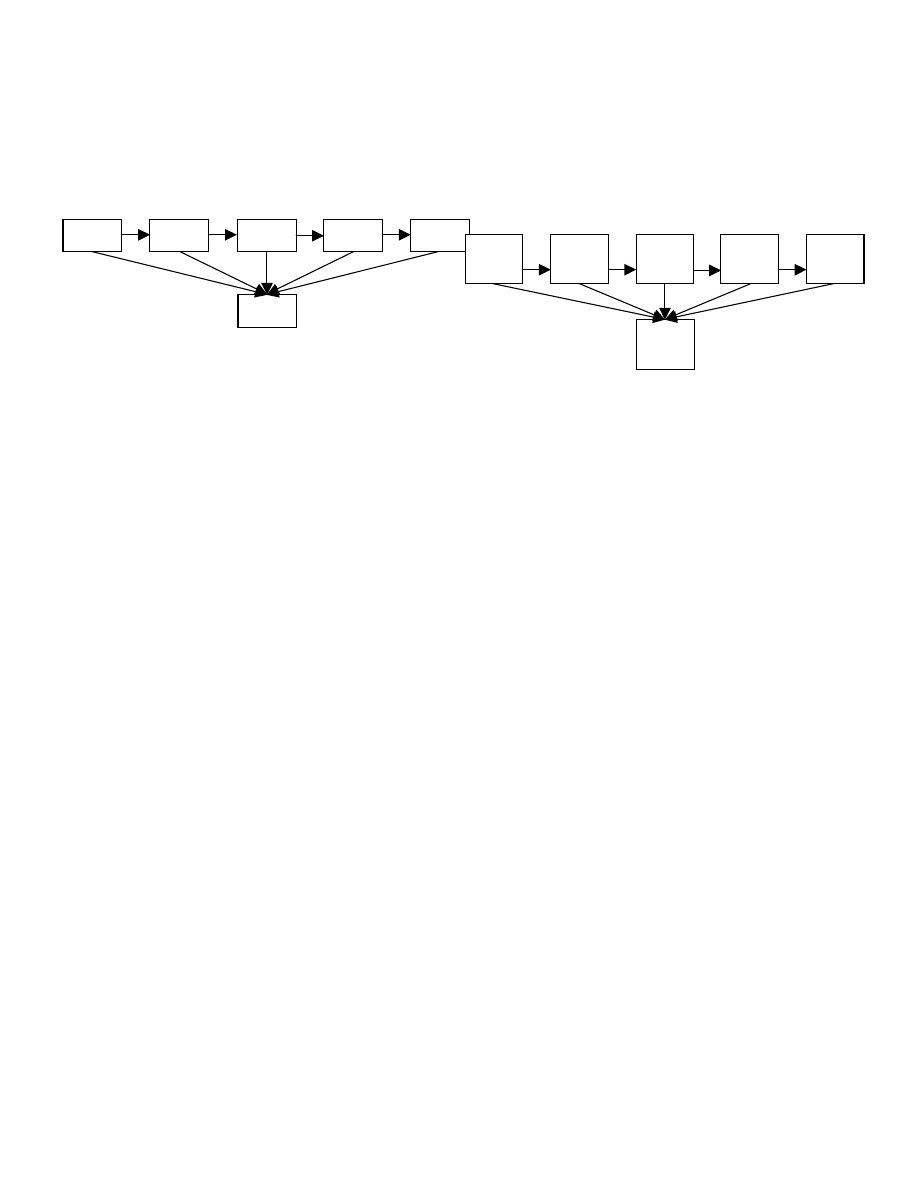
pseudo code. An example transition might be to send an ICMP Echo
Request message to the target host and evaluate the response. If an
ICMP Echo Reply is returned before the timeout period occurs,
move h into the next set to be further processed. Otherwise, discard
h (i.e., move it to the Fail set). Likewise, each h is moved from one
set to the next in the worm algorithm until it reaches the final set, IS,
or it is discarded.

Figure 4

4.2 Modeling Target Host State

A target host can be modeled as a state machine. The states of the
target host are S = {TS, VIS, VULN, AS, IS, FAIL}, meaning that
the target host is in the worm agent’s Target Set, Visible Set,
Vulnerable Set, Attack Set, Infection Set, and no set, respectively.
The start state S

= {TS}. The final states are S

= {FAIL, INF},

where INF is the accept state. The alphabet is Σ = {TRUE, FALSE}.
The state transition mapping provides an ordering over the states.
The states are linearly reached, excepting the FAIL state: ∂ = TS x
TRUE Æ VIS, VIS x TRUE Æ VULN, VULN x TRUE Æ AS, AS
x TRUE Æ IS. From any state on a FALSE, the transition is to
move to the FAIL state. The state machine model of the target host
can reflect either the worm's perspective of the target host's state or
the actual state of the target host. This state machine model makes
explicit the process that a worm goes through in learning about
targets and determining what can be done over (or to) that host.

4.3 Model For Perceived Worm State

The state of a worm agent is described by a tuple of sets: <TS, VIS,
VULN, AS, IS, FAIL>. Each set contains target hosts whose current
state is the name of the respective worm set. That is, all target hosts
that are (represented in the worm as being) in state TS are in the TS
set of the worm, all target hosts in state VIS are in the worm set VIS,
and so forth. In most instances of worm agents, a target host is in at
most one set at a time, such that the tuple of sets is itself a set and
the subsets are partitions of the complete set.
Some worms deviate on the number and sequence of states by
omitting actions and decisions thereby combining adjacent states.
Logically, aggregations of states do not affect the relative ordering
of states. A transition from one state to the next is only necessary if
an action is performed on the environment whose effect is used in
making a decision as to how to proceed. For example, it is common
for worms to not check whether an attack was effective before
attempting infection. This is usually the case with worms that use
buffer overflows as the exploit and infection mechanism where, as
discussed previously, a single, atomic action can accomplish both.
In some cases, several states are combined into one. In such a case,
the AS state and IS state are combined and the transition to it is the
value of the effect performed on the transition from the previous
state, VIS. The Slammer Worm is another example where states are
aggregated. Slammer did not check for visibility, vulnerability,
attackability, or infectability before launching a single packet that
did all of those in one step. In this case, there were only two states in
the linear process, TS and IS.

Figure 5 shows the state of a worm that has chosen to target hosts
h

.. h

. h

and h

have been determined to not be infectable for some

reason and are ignored. h

has been successfully infected. Privileges

have been acquired on h

via some attack, but it has not yet been

infected. h

has been determined to be vulnerable to some exploit

possessed by the worm agent. h

and h

are both visible to the worm

agent. Nothing can be said about h

at this time, other than that the

worm agent is targeting it.

Figure 5

Each action performed with respect to a single target host is totally
ordered and is defined by the particular implementation of the
worm. However, actions performed across target hosts may or may
not be totally ordered. A worm agent may be multithreaded or have
some other design that allows concurrent processing of various
targets. By augmenting the model with the notion of absolute time, a
total ordering can be applied to the transitions performed. Each
transition is annotated with a duration time. If the transitions can be
concurrent across target hosts, then the transition is also annotated
with a rate. These times may be dictated by resource constraints (i.e.,
processing time, network bandwidth, etc.) or logical constraints (i.e.,
flow control established by the worm author). For example, a ping
action may start at time t and complete at time t + 30 (in units of
milliseconds) if happening alone or t + 60 if happening in the
presence of several other pings. Likewise, pings might be sent
concurrently at a rate of 1000 times per second, for example. A
vulnerability scan might be in the range of milliseconds to seconds
depending on the scan. Another type of constraint might be how
many can be outstanding at a single time. A worm agent may not be
able to support more than 256 TCP connections at any one time. By
accounting for these resource and logical constraints in the model,
we can describe the behavior of a worm with respect to time. Also,
any initialization time can also be accounted for in the extended
worm set.
A worm agent changes state by continuing the worm algorithm with
respect to some target host, evaluating the effects of the behavior
initiated, and reflectively advancing the state of the target host and
subsequently its own state. It should be noted here that a worm may
assume that a transition was effective when, in reality, the transition
failed. The state of the worm, therefore, is a reflection of the worm’s
perception of the environment and not the actual state of the
environment. We call this the perceived state of the worm as it is the
worm’s perception of reality. Erroneous evaluations of the
effectiveness of transitions leads to inconsistency between the state
of the environment as the perceived state of the worm and the actual
state of the worm. Therefore, it is important to distinguish between
the worm’s perceived state from the worm’s actual state.

4.4 Model For Actual Worm State

The difference between the Turing Machine that represents the
worm’s perceived state and the Turing Machine that represents the
worm’s actual state is that the worm’s actual state reflects the actual
state of the environment as the worm would perceive it if it had

VIS

VULN

Fail

VIS

, h

VULN

Fail

, h

perfect knowledge. Whereas the perceived state of a worm reflects
the state of the environment as the worm perceives it, the actual state
of a worm reflects those attributes in the environment that are
relevant to the worm algorithm and are grounded in truth. Such an
idealistic machine is useful in predicting the potency of the
represented worm in a specific environment in a simulation.
Because the state of the Turing Machine is a tuple of states, where
target hosts move from one state to the next, we can represent the
logic of a worm with temporally extended sets. Temporally extended
sets are sets where the relational expression holds true over the
respective sets and an element from one set can move to the next set
of the next relational expression is true according to the temporal
requirements that separate the sets.

4.5 Temporally Extended Worm Sets

In the following sample extended worm set D represents duration of
time it takes for transition to take place and R represents the rate at
which transitions can take place. Both parameters refer to the
preceding transition (except for the initialization). The specific
values for D and R may vary according to the environment and
infected host. Representing the times as functions of the
environment, therefore, will provide greater fidelity. Time units are
omitted. Parenthetical statements are comments explaining the line.
Curly braces contain the logic of the worm sets and are in set
theoretic notation. For brevity only the new constraints placed at
each transition are presented (all previous constraints are also
necessarily true).

D: 0.5 (Initialization takes half a time unit)

TS = {h | h = (h

* a + b) mod n, for some constants a, b, n, and where h

the value of the previous iteration}

D: 0.0 (The calculation is practically immediate)

R: 0.0001 (10000 targets enumerated per unit time)

VIS = {h | TCP connect to host h:80 returns TRUE}

D: 0.03 (The time for a TCP connection setup)

R: 0.01 (100 targets can be pinged per time unit)

VULN/AS = {h | IIS exploit on h is successful and acquires elevated

privileges, the TCP session with h is still valid}

D: 0.03 , R: 0.05

IS = {h | the commands to download, install, and execute worm code

succeed}

D: 1.0 , R: 0.05

In the example above, the algorithm is concurrent. The Vulnerability
and Attack Sets are combined because there is no effort to determine
vulnerability before attacking. The worm’s perceived extended sets
would be similar, where the relational constraints would reflect the
worm’s perception.
The temporally extended worm sets can be used to evaluate not only
the potency of a worm in terms of its infection set, but also in terms
of its performance within a network. This also allows for
determining the effects of countermeasures imposed by a defender.
Therefore the contribution of the Turing Machine model of worms
and the subsequent temporally extended worm sets is the ability to
evaluate the outcomes of dynamic worm conflict.

4.6 Worm Collective State

The state of the worm collective can be modeled as a Turing
Machine with the same sets as a worm agent. Informally, the state of
the worm collective can be represented as the superset of each of the
worm sets of the individual worm agents. That is, the target set of
the collective TS’ = TS

U TS

U … U TS

, where TS

is the i

worm agent in the collective, and so forth for the other sets. This is

true for both the worm collective’s perceived state and the worm
collective’s actual state.
The formulation of the worm algorithm, the worm sets, and worm
state above, allowing some permutations, is sufficiently general to
assist in discreet temporal reasoning about network worms. While
the previous section provided the tools to reason about worms in a
static environment, this section presented tools that enable the
development of rich simulations that capture metrics of potency and
the temporal aspects of such behavior. We assert that the modeling
framework described above provides generality and richness in
reasoning about the network worm threat. In support of this claim
we provide the representations of a handful of worms in the next
section.

5. REPRESENTATIONS OF
CONTEMPORARY WORMS

In this section, we provide the worm algorithm and extended worm
sets for a handful of contemporary worms. The following worms
will be discussed in this section: Lion Worm, Code Red (the
original), Code Red II (a.k.a. CRvII), and Slammer (a.k.a. Sapphire).
Worm implementations can be arbitrarily complex. For each of
these worms we argue that the worm sets and worm algorithm are a
succinct and sufficiently correct representation of the worm to
evaluate its potency in a specific network.

5.1 Lion Worm

An analysis of the Lion Worm’s algorithm can be found at [15]. The
analysis provides a process flowchart for instances of the Lion
Worm. We provide the source code for this first example to better
show relationship to the worm algorithm. The worm is essentially
encoded into two threaded subprocesses: scan.sh and hack.sh with a
file called bindname.log as the communication medium between
them. Data flows unidirectionally from scan.sh to hack.sh. (The
other two subprocesses [1i0n.sh and star.sh] are control processes
and only affect the local machine and not the worm sets or
algorithm). The two relevant subprocesses are provided below in C-
like pseudo code.

The pseudocode for the Lion Worm that follows is simply a
reduction of the original source code (scan.sh and hack.sh),
modified for readability. Tabs are used to indicate scope.

scan.sh

forever

h = TAF( ) ; # TS = the enumeration of randb( );
If( TCP_Connect( h , 53 ) ) # attempt connect to h on port 53
write h to bindname.log ;

hack.sh

forever
get last 10 t from bindname.log #possible lapses and repeats
foreach h do
foreach exploit do {#note, there was only one exploit
if( TCP_Connect( h , 53 ) )#this is the one exploit
attack t with bindx.sh ;
execute "lynx -source http://207.181.140.2:27374 \
> 1i0n.tar;./lion"

These two processes can be represented as a single linear process
over hosts without loss of correctness since the hosts are indeed

processed in hack.sh linearly. The linear process is the Lion-specific
worm algorithm. The Lion Worm Algorithm follows. The
concurrent implementation decouples the checks for visibility and
vulnerability from the attack and infection.
The Lion Worm algorithm is succinctly described as:

forever
h = TAF( ) ;

# TAF

if( !TCP_Connect( h , 53 ) ) continue ;

# VIS/VULN

foreach exploit in ES do
attack h with exploit ;

# AS

download 1i0n to h from 207.181.140.2:27374 using lynx;
execute 1i0n

# IS

The Lion Worm algorithm is a constrained version of the general
worm algorithm. The TAF is constrained to target only values in the
enumeration of randb (the exact algorithm for randb is not
provided). The checks for visibility and vulnerability are performed
in one operation and returns TRUE whenever the target host has a
visible service running on TCP port 53. There is only one exploit
used to attack, and it is used against every visible target. The
infection phase occurs immediately after the attack using the remote
root shell (the result of an effective bindx.sh attack) to get the target
machine to download the worm code and execute it.
The Lion Worm Sets can be extracted from the Lion Worm
algorithm. The Target Set is simply an enumeration of all hosts
generated by randb. Since there is only one action whose effect is to
identify a visible and/or vulnerable host, the Visibility and
Vulnerability Sets contain the same hosts and are, therefore, the
same set. Note also that there is no control flow separating the attack
from the infection attempt. Although the two processes are distinct
in the algorithm and logically different, the Lion Worm Algorithm
does not have any check to see if the attack was successful before
moving on the infection attempt. The affects of this decision are that
the infection is attempted against machines indiscriminately for
which a TCP connection was established, regardless of the
effectiveness of the attack. Although there may be a difference
between the number of hosts that are effectively attacked and the
number of hosts that are infected (e.g., if there are vulnerable hosts
that don’t have lynx installed), the state of the worm is not reflected
by the distinction. The Lion Worm sets are:

TS = { h | h is generated by randb }
VIS/VULN = { h | h in TS, h:TCP/53 is visible to localhost }
AS = {h | h in VIS/VULN, and h runs a vulnerable version of bind }
IS = { h | h in AS, lynx is installed and executable, 207.181.140.2:27374 is

visible to h, 1i0n can be installed and executed}

Given an initial infection set and an environment the sets above
could be used to generate the subsequent Worm Coverage Transitive
Closure. The Lion Worm extended sets follow. (The time units are
for illustrative purposes only and are probably not accurate,
although the logic is correct.)

D: 0.0 (Time to initialization)

TS = { h | h is generated by randb }

D: 0.0 (Time to generate h)

R: 0.001 (1000 targets can be generated per unit time)

VIS/VULN = { h | h in TS, h:TCP/53 is visible to localhost }

D: 2.5 * RTT (Time to open and close TCP connection)

AS = {h | h in VIS/VULN, and h runs a vulnerable bind service}

D: 2.5 * RTT (Setup TCP connection and run exploit)

IS = { h | h in AS, lynx is installed and executable, 207.181.140.2:27374 is

visible to h, 1i0n can be installed and executed}

D: 3.5 * RTT + 0.1

(Time to issue command to download,

install, and execute worm code)

The RTT refers to the round-trip time (RTT) of a pair of hosts in a
network. This representation is sufficient for calculating the spread
rate and other time-relevant metrics for the Lion Worm.

5.2 Code Red I

The Code Red I extended worm sets are provided here and are
derived from an analysis of Code Red I by eEye (http://
www.eeye.com/html/Research/Advisories/AL20010717.html). One
interesting feature of this worm is the modification to the
performance of the loop based on local information. During
initialization, the worm checks the infected machine’s locale. If the
locale is English, twice as many threads are spawned (300) as there
are if the locale is Chinese (150).

Initialize:

D: 0.0 (Check to see if local host is infected)

R: 300 (English locale) or 150 (Chinese locale)

Populate TS: D(insignificant)

TS = {h | h generated by rand( fixed_seed )}, thus TS is an ordered list that

and is the same across all worm agents

D: 1.5 * RTT (TCP connection setup)

VIS/VULN = {h | h in TS, and TCP_Connect with h succeeded}

D: 0.5 * RTT (Send HTTP_GET_Exploit)

AS= {h | h in VIS/VULN, and HTTP_GET_Exploit connection succeeded}

D: 0.5 * RTT (Receive response to exploit)

IS = {h | h in VIS/VULN, and Receive_Return_GET}

D: 0.01 (The time it takes to execute)

One interesting point about this worm is the choice of a fixed seed
for the TAF. Subsequently, every instance of this worm targets the
exact same sequence of hosts in the exact same order. Effectively,
only one infected machine infects other machines.

5.3 Code Red II

The Code Red II extended worm sets are provided here and are
derived from an analysis of Code Red II by eEye (http://
www.eeye.com/html/Research/Advisories/AL20010804.html).

Initialize:

D: 0.0 (Check to see if local host is infected)

R: 300 (English locale) or 150 (Chinese locale)

TS = {h | h has address X.Y where X is the same netmask as the local host,

|X|+|Y|=32, and |X| follows this probability distribution (|X|,P): (0, 0.125), (8,

0.50), (16, 0.375), and X.Y != 127.* or 224.*

D: 1.5 * RTT (Set up TCP connection)

VIS/VULN = {h | h in TS, and TCP_Connect with h succeeded}

D: 0.5 * RTT (Send HTTP_GET_Exploit)

AS/IS= {h | h in VIS/VULN, and HTTP_GET_Exploit connection

succeeded}

D: 0.1 + 1.0 * RTT

(Time to install, execute worm code plus

time to tear down TCP connection)

5.4 Slammer/Sapphire

The pseudo code for Slammer is as follows.

forever
T = TAF( ) ; #uses linear congruence

# TAF

create UDP packet to T on port 1434 with exploit; #VIS/VULN/AS/IS

The Slammer Worm algorithm is different from the previous
examples as it does not place any constraints on the targets. Also, as

the vulnerable service being targeted is UDP-based, there is no
overhead associated with creating a session. The result is a compact
worm that spreads quickly and targets many hosts that either do not
exist or are not vulnerable. The extended worm sets are as follows.

D: 0.0 (Initialization time is inconsequential)

TS = { h | h is generated by one of the linear congruences
h' = (h * 214013 – (0xffd9613c XOR 0x77f8313c) ) mod 2^32
h' = (h * 214013 – (0xffd9613c XOR 0x77e89b18) ) mod 2^32
h' = (h * 214013 – (0xffd9613c XOR 0x77ea094c) ) mod 2^32
h

is produced by getTick( ) from the Windows API }

R: bandwidth/376 bytes

VIS/VULN/AS/IS = { h | h in TS, h.UDP/1434 is visible to localhost, h runs

Microsoft SQL Server 2000 or MSDE 2000, h runs the Windows operating

system }

D: 0.0 (creating and sending a packet are relatively immediate)

The linear congruences in TS are described in
http://www.caida.org/outreach/papers/2003/sapphire/sapphire.html.
The linear congruences have not been verified by the authors of this
paper.
From looking at the time annotated worm sets for Slammer, it is
clear that it will spread much more quickly than previous worms
given the same vulnerability density and topology. The benefit in
using UDP (greatly reduced latency between hosts). Also, it makes
the attacks concurrent, being limited only by the bandwidth
available to the host.

6. CONCLUSIONS & FUTURE WORK

In this paper we have presented a description of network worms. We
have provided a relational model that describes the relationship
between a worm’s parameters, the environment, and the worm’s
potency. The Worm Coverage Transitive Closure (WCTC) is a
computation of a worm’s final infection set given its parameters and
operating environment. Based on current defensive technology, the
WCTC is adequate to describe a worm’s potency with respect to a
particular environment because there are no defensive
countermeasures that respond within the time scale of most worm
conflicts. We also present a generalized worm algorithm and a
model for worm state that can be used to succinctly capture the
germane attributes of a worm that affect its potency. The model can
be used to develop simulations for evaluating the temporal aspects
of worm potency as well as evaluate the effects of modifications to
defensive tactics and postures. As this model clearly defines what
parameters affect worm potency, we expect it will be a useful tool
for identifying and evaluating defensive tactics and postures for both
static and dynamic worm conflict.
We are currently implementing this model in the EASEL modeling
and simulation environment. We will use that model to evaluate
worm detection and response capabilities.

7. ACKNOWLEDGEMENTS

Appreciation is extended to Sushil Jajodia, Paul Ammann, Amgad
Fayad, Dale Johnson, Nicholas Weaver, and several other MITRE

employees who commented on the model and provided suggestions
for improvement.

8. REFERENCES

[1]

http://www.cert.org/body/advisories/CA200126_FA200126.ht
ml

[2]

Fred Cohen, “Computer Viruses: Theory and Experiments”,
Computers and Security, Volume 6, Number 1, January, 1987,
pp 22-35.

[3]

Fred Cohen, “A Formal Definition of Computer Worms and
Some Related Results”, Computers and Security, Volume 11,
Number 7, November, 1992, pp 641-652.

[4]

Stuart Staniford-Chen, R. Crawford, M. Dilger, J. Frank, J.
Hoagland, K. Levitt, D. Zerkle, “GrIDS A Graph-Based
Intrusion Detection System for Large Networks”, In the
Proceedings of the 19th National Information Systems Security
Conference, 1996.

[5]

Robert Baldwin, Rule Based Analysis of Computer Security.
PhD Thesis, MIT EE, June 1987.

[6]

Dan Zerkle, Karl Levitt, “NetKuang -- A Multi-Host
Configuration Vulnerability Checker”, In 6th USENIX
Security Symposium, San Jose, California, July 1996.

[7]

Paul Ammann, Duminda Wijesekera, Saket Kaushik,
“Scalable, Graph-based Network Vulnerability Analysis”,
ACM CCS 2002, November 18-22, 2002, Washington, DC.

[8]

Oleg Sheyner, Somesh Jha, Jeannette M. Wing, “Automated
Generation and Analysis of Attack Graphs”, Proceedings of the
IEEE Symposium on Security and Privacy, Oakland, CA, May
2002.

[9]

J. O. Kephat, S. R. White, “Directed-graph Epidemiological
Models of Computer Viruses”, Proceedings of the 1991 IEEE
Computer Society Symposium on Research in Security and
Privacy, pp. 343-359.

[10]

J. O. Kephart, S. R. White, and Chess, “Computers and
Epidemiology”, IEEE Spectrum, May 1993.

[11]

Stuart Staniford, Vern Paxson, Nicholas Weaver, “How to 0wn
the Internet in Your Spare Time”, Proceedings of the 11th
USENIX Security Symposium 2002.

[12]

Cliff Changchun Zou, Weibo Gong, Don Towsley, “Code Red
Worm Propagation Modeling and Analysis”, ACM CCS 2002,
November 18-22, 2002, Washington, DC.

[13]

Chenxi Wang, John Knight, Matthew Elder, “On Computer
Viral Infection and the Effect of Immunization”, ACSAC
2000, pp 246-25.

[14]

http://www.sophos.com/virusinfo/analyses/w32nachia.html

[15]

http://www.whitehats.com/library/worms/lion/