
Chapter 1
HEAVY TAILS IN FINANCE FOR INDEPENDENT
OR MULTIFRACTAL PRICE INCREMENTS
BENOIT B. MANDELBROT
Sterling Professor of Mathematical Sciences, Yale University, New Haven, CT 065020-8283, USA
Contents
Abstract
4
1. Introduction: A path that led to model price by Brownian motion (Wiener or
fractional) of a multifractal trading time
5
1.1. From the law of Pareto to infinite moment “anomalies” that contradict the Gaussian “norm”
5
1.2. A scientific principle: scaling invariance in finance
6
1.3. Analysis alone versus statistical analysis followed by synthesis and graphic output
7
1.4. Actual implementation of scaling invariance by multifractal functions: it requires additional
assumptions that are convenient but not a matter of principle, for example, separability and
compounding
7
2. Background: the Bernoulli binomial measure and two random variants: shuffled
and canonical
8
2.1. Definition and construction of the Bernoulli binomial measure
8
2.2. The concept of canonical random cascade and the definition of the canonical binomial measure
9
2.3. Two forms of conservation: strict and on the average
9
2.4. The term “canonical” is motivated by statistical thermodynamics
10
2.5. In every variant of the binomial measure one can view all finite (positive or negative) powers
together, as forming a single “class of equivalence”
10
2.6. The full and folded forms of the address plane
11
2.7. Alternative parameters
11
3. Definition of the two-valued canonical multifractals
11
3.1. Construction of the two-valued canonical multifractal in the interval
[0, 1]
11
3.2. A second special two-valued canonical multifractal: the unifractal measure on the canonical
Cantor dust
12
3.3. Generalization of a useful new viewpoint: when considered together with their powers from
−∞ to ∞, all the TVCM parametrized by either p or 1 − p form a single class of equivalence
12
3.4. The full and folded address planes
12
3.5. Background of the two-valued canonical measures in the historical development of multi-
fractals
13
Handbook of Heavy Tailed Distributions in Finance, Edited by S.T. Rachev
© 2003 Elsevier Science B.V. All rights reserved

2
B.B. Mandelbrot
4. The limit random variable Ω
= µ([0, 1]), its distribution and the star functional
equation
13
4.1. The identity EM
= 1 implies that the limit measure has the “martingale” property, hence
the cascade defines a limit random variable Ω
= µ([0, 1])
13
4.2. Questions
14
4.3. Exact stochastic renormalizability and the “star functional equation” for Ω
14
4.4. Metaphor for the probability of large values of Ω, arising in the theory of discrete time
branching processes
14
4.5. To a large extent, the asymptotic measure Ω of a TVCM is large if, and only if, the pre-fractal
measure µ
k
(
[0, 1]) has become large during the very first few stages of the generating cascade
15
5. The function τ (q): motivation and form of the graph
15
5.1. Motivation of τ (q)
15
5.2. A generalization of the role of Ω: middle- and high-frequency contributions to microran-
domness
15
5.3. The expected “partition function”
Eµ
q
(
d
i
t)
16
5.4. Form of the τ (q) graph
17
5.5. Reducible and irreducible canonical multifractals
18
6. When u > 1, the moment EΩ
q
diverges if q exceeds a critical exponent q
crit
satisfying τ (q)
= 0; Ω follows a power-law distribution of exponent q
crit
18
6.1. Divergent moments, power-law distributions and limits to the ability of moments to deter-
mine a distribution
18
6.2. Discussion
19
6.3. An important apparent “anomaly”: in a TVCM, the q-th moment of Ω may diverge
19
6.4. An important role of τ (q): if q > 1 the q-th moment of Ω is finite if, and only if, τ (q) > 0;
the same holds for µ(dt) whenever dt is a dyadic interval
19
6.5. Definition of q
crit
; proof that in the case of TVCM q
crit
is finite if, and only if, u > 1
20
6.6. The exponent q
crit
can be considered as a macroscopic variable of the generating process
20
7. The quantity α: the original Hölder exponent and beyond
21
7.1. The Bernoulli binomial case and two forms of the Hölder exponent: coarse-grained (or
coarse) and fine-grained
21
7.2. In the general TVCM measure, α
= ˜α, and the link between “α” and the Hölder exponent
breaks down; one consequence is that the “doubly anomalous” inequalities α
min
<
0, hence
˜α < 0, are not excluded
22
8. The full function f (α) and the function ρ(α)
23
8.1. The Bernoulli binomial measure: definition and derivation of the box dimension function
f (α)
23
8.2. The “entropy ogive” function f (α); the role of statistical thermodynamics in multifractals
and the contrast between equipartition and concentration
23
8.3. The Bernoulli binomial measure, continued: definition and derivation of a function ρ(α)
=
f (α)
− 1 that originates as a rescaled logarithm of a probability
24
8.4. Generalization of ρ(α) to the case of TVCM; the definition of f (α) as ρ(α)
+ 1 is indirect
but significant because it allows the generalized f to be negative
24
8.5. Comments in terms of probability theory
25

Ch. 1:
Heavy Tails in Finance for Independent or Multifractal Price Increments
3
8.6. Distinction between “center” and “tail” theorems in probability
26
8.7. The reason for the anomalous inequalities f (α) < 0 and α < 0 is that, by the definition of a
random variable µ(dt), the sample size is bounded and is prescribed intrinsically; the notion
of supersampling
26
8.8. Excluding the Bernoulli case p
= 1/2, TVCM faces either one of two major “anomalies”:
for p >
−1/2, one has f (α
min
)
= 1 + log
2
p >
0 and f (α
max
)
= 1 + log
2
(
1
− p) < 0; for
p <
1/2, the opposite signs hold
27
8.9. The “minor anomalies” f (α
max
) >
0 or f (α
min
) >
0 lead to sample function with a clear
“ceiling” or “floor”
27
9. The fractal dimension D
= τ
(
1)
= 2[−pu log
2
u
− (1 − p)v log
2
v
] and mul-
tifractal concentration
27
9.1. In the Bernoulli binomial measures weak asymptotic negligibility holds but strong asymp-
totic negligibility fails
28
9.2. For the Bernoulli or canonical binomials, the equation f (α)
= α has one and only one solu-
tion; that solution satisfies D > 0 and is the fractal dimension of the “carrier” of the measure
28
9.3. The notion of “multifractal concentration”
29
9.4. The case of TVCM with p < 1/2, allows D to be positive, negative, or zero
29
10. A noteworthy and unexpected separation of roles, between the “dimension
spectrum” and the total mass Ω; the former is ruled by the accessible α for
which f (α) > 0, the latter, by the inaccessible α for which f (α) < 0
30
10.1. Definitions of the “accessible ranges” of the variables: qs from q
∗
min
to q
∗
max
and αs from
α
∗
min
to α
∗
max
; the accessible functions τ
∗
(q)
and f
∗
(α)
30
10.2. A confrontation
30
10.3. The simplest cases where f (α) > 0 for all α, as exemplified by the canonical binomial
31
10.4. The extreme case where f (α) < 0 and α < 0 both occur, as exemplified by TVCM when
u >
1
31
10.5. The intermediate case where α
min
>
0 but f (α) < 0 for some values of α
31
11. A broad form of the multifractal formalism that allows α < 0 and f (α) < 0
31
11.1. The broad “multifractal formalism” confirms the form of f (α) and allows f (α) < 0 for
some α
32
11.2. The Legendre and inverse Legendre transforms and the thermodynamical analogy
32
Acknowledgments
32
References
32

4
B.B. Mandelbrot
Abstract
This chapter has two goals. Section 1 sketches the history of heavy tails in finance through
the author’s three successive models of the variation of a financial price: mesofractal,
unifractal and multifractal. The heavy tails occur, respectively, in the marginal distribution
only (Mandelbrot, 1963), in the dependence only (Mandelbrot, 1965), or in both (Mandel-
brot, 1997). These models increase in the scope of the “principle of scaling invariance”,
which the author has used since 1957.
The mesofractal model is founded on the stable processes that date to Cauchy and Lévy.
The unifractal model uses the fractional Brownian motions introduced by the author. By
now, both are well-understood.
To the contrary, one of the key features of the multifractals (Mandelbrot, 1974a, b) re-
mains little known. Using the author’s recent work, introduced for the first time in this
chapter, the exposition can be unusually brief and mathematically elementary, yet covering
all the key features of multifractality. It is restricted to very special but powerful cases:
(a) the Bernoulli binomial measure, which is classical but presented in a little-known fash-
ion, and (b) a new two-valued “canonical” measure. The latter generalizes Bernoulli and
provides an especially short path to negative dimensions, divergent moments, and divergent
(i.e., long range) dependence. All those features are now obtained as separately tunable as-
pects of the same set of simple construction rules.

Ch. 1:
Heavy Tails in Finance for Independent or Multifractal Price Increments
5
My work in finance is well-documented in easily accessible sources, many of them repro-
duced in Mandelbrot (1997 and also in 2001a, b, c, d). That work having expanded and
been commented upon by many authors, a survey of the literature is desirable, but this is
a task I cannot undertake now. However, it was a pleasure to yield to the entreaties of this
Handbook’s editors by a text in which a new technical contribution is preceded by an in-
troductory sketch followed by a simple new presentation of an old feature that used to be
dismissed as “technical”, but now moves to center stage.
The history of heavy tails in finance began in 1963. While acknowledging that the suc-
cessive increments of a financial price are interdependent, I assumed independence as a
first approximation and combined it with the principle of scaling invariance. This led to
(Lévy) stable distributions for the price changes. The tails are very heavy, in fact, power-
law distributed with an exponent α < 2.
The multifractal model advanced in Mandelbrot (1997) extends scale invariance to allow
for dependence. Readily controllable parameters generate tails that are as heavy as desired
and can be made to follow a power-law with an exponent in the range 1 < α <
∞. This last
result, an essential one, involves a property of multifractals that was described in Mandel-
brot (1974a, b) but remains little known among users. The goal of the example described
after the introduction is to illustrate this property in a very simple form.
1. Introduction: A path that led to model price by Brownian motion (Wiener or
fractional) of a multifractal trading time
Given a financial price record P (t) and a time lag dt , define L(t, dt)
= log P (t + dt) −
log P (t). The 1900 dissertation of Louis Bachelier introduced Brownian motion as a model
of P (t). In later publications, however, Bachelier acknowledged that this is a very rough
first approximation: he recognized the presence of heavy tails and did not rule out depen-
dence. But until 1963, no one had proposed a model of the heavy tails’ distribution.
1.1. From the law of Pareto to infinite moment “anomalies” that contradict the Gaussian
“norm”
All along, search for a model was inspired by a finding rooted in economics outside of
finance. Indeed, the distribution of personal incomes proposed in 1896 by Pareto involved
tails that are heavy in the sense of following a power-law distribution Pr
{U > u} = u
−α
.
However, almost nobody took this income distribution seriously. The strongest “conven-
tional wisdom” argument against Pareto was that the value α
= 1.7 that he claimed leads
to the variance of U being infinite.
Infinite moments have been a perennial issue both before my work and (unfortunately)
ever since. Partly to avoid them, Pareto volunteered an exponential multiplier, resulting in
Pr
{U > u} = u
−α
exp(
−βu).

6
B.B. Mandelbrot
Also, Herbert A. Simon expressed a universally held view when he asserted in 1953 that
infinite moments are (somehow) “improper”. But in fact, the exponential multipliers are
not needed and infinite moments are perfectly proper and have important consequences. In
multifractal models, depending on specific features, variance can be either finite or infinite.
In fact, all moments can be finite, or they can be finite only up to a critical power q
crit
that
may be 3, 4, or any other value needed to represent the data.
Beginning in the late 1950s, a general theme of my work has been that the uses of sta-
tistics must be recognized as falling into at least two broad categories. In the “normal”
category, one can use the Gaussian distribution as a good approximation, so that the com-
mon replacement of the term, “Gaussian”, by “normal” is fully justified. To the contrary,
in the category one can call “abnormal” or “anomalous”, the Gaussian is very misleading,
even as an approximation.
To underline this distinction, I have long suggested – to little effect up to now – that the
substance of the so-called ordinary central limit theorem would be better understood if it
is relabeled as the center limit theorem. Indeed, that theorem concerns the center of the
distribution, while the anomalies concern the tails. Following up on this vocabulary, the
generalized central limit theorem that yields Lévy stable limits would be better understood
if called a tail limit theorem. This distinction becomes essential in Section 8.5.
Be that as it may, I came to believe in the 1950s that the power-law distribution and
the associated infinite moments are key elements that distinguish economics from classical
physics. This distinction grew by being extended from independent to highly dependent
random variables. In 1997, it became ready to be phrased in terms of randomness and
variability falling in one of several distinct “states”. The “mild” state prevails for classical
errors of observation and for sequences of near-Gaussian and near-independent quantities.
To the contrary, phenomena that present deep inequality necessarily belong to the “wild”
state of randomness.
1.2. A scientific principle: scaling invariance in finance
A second general theme of my work is the “principle” that financial records are invariant by
dilating or reducing the scales of time and price in ways suitably related to each other. There
is no need to believe that this principle is exactly valid, nor that its exact validity could ever
be tested empirically. However, a proper application of this principle has provided the
basis of models or scenarios that can be called good because they satisfy all the following
properties:
(a) they closely model reality,
(b) they are exceptionally parsimonious, being based on very few very general a priori
assumptions, and
(c) they are creative in the following sense: extensive and correct predictions arise as con-
sequences of a few assumptions; when those assumptions are changed the consequences
also change. By contrast, all too many financial models start with Brownian motion,
then build upon it by including in the input every one of the properties that one wishes
to see present in the output.

Ch. 1:
Heavy Tails in Finance for Independent or Multifractal Price Increments
7
1.3. Analysis alone versus statistical analysis followed by synthesis and graphic output
The topic of multifractal functions has grown into a well-developed analytic theory, making
it easy to apply the multifractal formalism blindly. But it is far harder to understand it and
draw consequences from its output. In particular, statistical techniques for handling multi-
fractals are conspicuous by their near-total absence. After they become actually available,
their applicability will have to be investigated carefully.
A chastening example is provided by the much simpler question of whether or not fi-
nancial series exhibit global (long range) dependence. My claim that they do was largely
based on R/S analysis which at this point relies heavily on graphical evidence. Lo (1991)
criticized this conclusion very severely as being subjective. Also, a certain alternative test
Lo described as “objective” led to a mixed pattern of “they do” and “they do not”. This
pattern being practically impossible to interpret, Lo took the position that the simpler out-
come has not been shown wrong, hence one can assume that long range dependence is
absent.
Unfortunately, the “objective test” in question assumed the margins to be Gaussian.
Hence, Lo’s experiment did not invalidate my conclusion, only showed that the test is
not robust and had repeatedly failed to recognize long range dependence.
The proper conclusion is that careful graphic evidence has not yet been superseded.
The first step is to attach special importance to models for which sample functions can be
generated.
1.4. Actual implementation of scaling invariance by multifractal functions: it requires
additional assumptions that are convenient but not a matter of principle, for
example, separability and compounding
By and large, an increase in the number and specificity in the assumptions leads to an
increase in the specificity of the results. It follows that generality may be an ideal unto
itself in mathematics, but in the sciences it competes with specificity, hence typically with
simplicity, familiarity, and intuition.
In the case of multifractal functions, two additional considerations should be heeded.
The so-called multifractal formalism (to be described below) is extremely important. But
it does not by itself specify a random function closely enough to allow analysis to be
followed by synthesis. Furthermore, multifractal functions are so new that it is best, in a
first stage, to be able to rely on existing knowledge while pursuing a concrete application.
For these and related reasons, my study of multifractals in finance has relied heavily on
two special cases.
One is implemented by the recursive “cartoons” investigated in Mandelbrot (1997) and
in much greater detail in Mandelbrot (2001c).
The other uses compounding. This process begins with a random function F (θ ) in which
the variable θ is called an “intrinsic time”. In the key context of financial prices, θ is
called “trading time”. The possible functions F (θ ) include all the functions that have been
previously used to model price variation. Foremost is the Wiener Brownian motion B(t)

8
B.B. Mandelbrot
postulated by Bachelier. The next simplest are the fractional Brownian motion B
H
(t)
and
the Lévy stable “flight” L(t).
A separate step selects for the intrinsic trading time a scale invariant random functions
of the physical “clock time” t . Mandelbrot (1972) recommended for the function θ (t) the
integral of a multifractal measure. This choice was developed in Mandelbrot (1997) and
Mandelbrot, Calvet and Fisher (1997).
In summary, one begins with two statistically independent random functions F (θ ) and
θ (t)
, where θ (t) is non-decreasing. Then one creates the “compound” function F
[θ(t)] =
ϕ(t)
. Choosing F (θ ) and θ (t) to be scale-invariant insures that ϕ(t) will be scale-invariant
as well. A limitation of compounding as defined thus far is that it demands independence
of F and θ , therefore restricts the scope of the compound function.
In a well-known special case called Bochner subordination, the increments of θ (t) are
independent. As shown in Mandelbrot and Taylor (1967), it follows that B
[θ(t)] is a Lévy
stable process, i.e., the mesofractal model. This approach has become well-known. The
tails it creates are heavy and do follow a power law distribution but there are at least two
drawbacks. The exponent α is at most 2, a clearly unacceptable restriction in many cases,
and the increments are independent.
Compounding beyond subordination was introduced because it allows α to take any
value > 1 and the increments to exhibit long term dependence. All this is discussed else-
where (Mandelbrot, 1997 and more recent papers).
The goal of the remainder of this chapter is to use a specially designed simple case to
explain how multifractal measure suffices to create a power-law distribution. The idea is
that L(t, dt)
= dϕ(t) where ϕ = B
H
[θ(t)]. Roughly, dµ(t) is |dB
H
|
1/H
. In the Wiener
Brownian case, H
= 1/2 and dµ is the “local variance”. This is how a price that fluctuates
up and down is reduced to a positive measure.
2. Background: the Bernoulli binomial measure and two random variants: shuffled
and canonical
The prototype of all multifractals is nonrandom: it is a Bernoulli binomial measure. Its
well-known properties are recalled in this section, then Section 3 introduces a random
“canonical” version. Also, all Bernoulli binomial measures being powers of one another,
a broader viewpoint considers them as forming a single “class of equivalence”.
2.1. Definition and construction of the Bernoulli binomial measure
A multiplicative nonrandom cascade. A recursive construction of the Bernoulli binomial
measures involves an “initiator” and a “generator”. The initiator is the interval
[0, 1] on
which a unit of mass is uniformly spread. This interval will recursively split into halves,
yielding dyadic intervals of length 2
−k
. The generator consists in a single parameter u,
variously called multiplier or mass. The first stage spreads mass over the halves of every
dyadic interval, with unequal proportions. Applied to
[0, 1], it leaves the mass u in [0, 1/2]

Ch. 1:
Heavy Tails in Finance for Independent or Multifractal Price Increments
9
and the mass v in
[1/2, 1]. The (k + 1)-th stage begins with dyadic intervals of length 2
−k
,
each split in two subintervals of length 2
−k−1
. A proportion equal to u goes to the left
subinterval and the proportion v, to the right.
After k stages, let ϕ
0
and ϕ
1
= 1 − ϕ
0
denote the relative frequencies of 0’s and 1’s in
the finite binary development t
= 0.β
1
β
2
. . . β
k
. The “pre-binomial” measures in the dyadic
interval
[dt] = [t, t + 2
−k
] takes the value
µ
k
(
dt)
= u
kϕ
0
v
kϕ
1
,
which will be called “pre-multifractal”. This measure is distributed uniformly over the
interval. For k
→ ∞, this sequence of measures µ
k
(
dt) has a limit µ(dt), which is the
Bernoulli binomial multifractal.
Shuffled binomial measure. The proportion equal to u now goes to either the left or
the right subinterval, with equal probabilities, and the remaining proportion v goes to the
remaining subinterval. This variant must be mentioned but is not interesting.
2.2. The concept of canonical random cascade and the definition of the canonical
binomial measure
Mandelbrot (1974a, b) took a major step beyond the preceding constructions.
The random multiplier M. In this generalization every recursive construction can be
described as follows. Given the mass m in a dyadic interval of length 2
−k
,
the two subin-
tervals of length 2
−k−1
are assigned the masses M
1
m
and M
2
m,
where M
1
and M
2
are
independent realizations of a random variable M called multiplier. This M is equal to u or
v
with probabilities p
= 1/2 and 1 − p = 1/2.
The Bernoulli and shuffled binomials both impose the constraint that M
1
+ M
2
= 1. The
canonical binomial does not. It follows that the canonical mass in each interval of duration
2
−k
is multiplied in the next stage by the sum M
1
+ M
2
of two independent realizations
of M. That sum is either 2u (with probability p
2
)
, or 1 (with probability 2(1
− p)p), or 2v
(with probability 1
− p
2
).
Writing p instead of 1/2 in the Bernoulli case and its variants complicates the nota-
tion now, but will soon prove advantageous: the step to the TVCM will simply consist in
allowing 0 < p < 1.
2.3. Two forms of conservation: strict and on the average
Both the Bernoulli and shuffled binomials repeatedly redistribute mass, but within a dyadic
interval of duration 2
−k
, the mass remains exactly conserved in all stages beyond the k-th.
That is, the limit mass µ(t) in a dyadic interval satisfies µ
k
(
dt)
= µ(dt).
In a canonical binomial, to the contrary, the sum M
1
+ M
2
is not identically 1, only its
expectation is 1. Therefore, canonical binomial construction preserve mass on the average,
but not exactly.

10
B.B. Mandelbrot
The random variable Ω. In particular, the mass µ(
[0, 1]) is no longer equal to 1. It is a
basic random variable denoted by Ω and discussed in Section 4.
Within a dyadic interval dt of length 2
−k
, the cascade is simply a reduced-scale version
of the overall cascade. It transforms the mass µ
k
(
dt) into a product of the form µ(dt)
=
µ
k
(
dt)Ω(dt) where all the Ω(dt) are independent realizations of the same variable Ω.
2.4. The term “canonical” is motivated by statistical thermodynamics
As is well known, statistical thermodynamics finds it valuable to approximate large systems
as juxtapositions of parts, the “canonical ensembles”, whose energy only depends on a
common temperature and not on the energies of the other parts. Microcanonical ensembles’
energies are constrained to add to a prescribed total energy. In the study of multifractals,
the use of this metaphor should not obscure the fact that the multiplication of canonical
factors introduces strong dependence among µ(dt) for different intervals dt .
2.5. In every variant of the binomial measure one can view all finite (positive or negative)
powers together, as forming a single “class of equivalence”
To any given real exponent g
= 1 and multipliers u and v corresponds a multiplier M
g
that
can take either of two values u
g
= ψu
g
with probability p, and v
g
= ψv
g
with probability
1
− p. The factor ψ is meant to insure pu
g
+ (1 − p)v
g
= 1/2. Therefore, ψ[pu
g
+
(
1
− p)v
g
] = 1/2, that is, ψ = 1/[2EM
g
]. The expression 2EM
g
will be generalized and
encountered repeatedly especially through the expression
τ (q)
= − log
2
pu
q
+ (1 − p)v
q
− 1 = − log
2
2EM
q
.
This is simply a notation at this point but will be justified in Section 5. It follows that
ψ
= 2
−τ(g)
, hence
u
g
= u
g
2
τ (g)
and
v
g
= v
g
2
τ (g)
.
Assume u > v. As g ranges from 0 to
∞, u
g
ranges from 1/2 to 1 and v
g
ranges from
1/2 to 0; the inequality u
g
> v
g
is preserved. To the contrary, as g ranges from 0 to
∞,
v
g
< u
g
. For example, g
= −1 yields
u
g
=
1/u
1/u
+ 1/v
= v and v
g
=
1/v
1/v
+ 1/v
= u.
Thus, inversion leaves both the shuffled and the canonical binomial measures un-
changed. For the Bernoulli binomial, it only changes the direction of the time axis.
Altogether, every Bernoulli binomial measure can be obtained from any other as a re-
duced positive or negative power. If one agrees to consider a measure and its reduced
powers as equivalent, there is only one Bernoulli binomial measure.

Ch. 1:
Heavy Tails in Finance for Independent or Multifractal Price Increments
11
In concrete terms relative to non-infinitesimal dyadic intervals, the sequences represent-
ing log µ for different values of g are mutually affine. Each is obtained from the special
case g
= 1 by a multiplication by g followed by a vertical translation.
2.6. The full and folded forms of the address plane
In anticipation of TVCM, the point of coordinates u and v will be called the address of a
binomial measure in a full address space. In that plane, the locus of the Bernoulli measures
is the interval defined by 0 < v, 0 < u, and u
+ v = 1.
The folded address space will be obtained by identifying the measures (u, v) and (v, u),
and representing both by one point. The locus of the Bernoulli measures becomes the
interval defined by the inequalities 0 < v < u and u
+ v = 1.
2.7. Alternative parameters
In its role as parameter added to p
= 1/2, one can replace u by the (“information-
theoretical”) fractal dimension D
= −u log
2
u
− v log
2
v
which can be chosen at will in
this open interval
]0, 1[. The value of D characterizes the “set that supports” the measure.
It received a new application in the new notion of multifractal concentration described in
Mandelbrot (2001c). More generally, the study of all multifractals, including the Bernoulli
binomial, is filled with fractal dimensions of many other sets. All are unquestionably posi-
tive. One of the newest features of the TVCM will prove to be that they also allow negative
dimensions.
3. Definition of the two-valued canonical multifractals
3.1. Construction of the two-valued canonical multifractal in the interval
[0, 1]
The TVCM are called two-valued because, as with the Bernoulli binomial, the multiplier M
can only take 2 possible values u and v. The novelties are that p need not be 1/2, the
multipliers u and v are not bounded by 1, and the inequality u
+ v = 1 is acceptable.
For u
+ v = 1, the total mass cannot be preserved exactly. Preservation on the average
requires
EM
= pu + (1 − p)v =
1
2
,
hence 0 < p
= (1/2 − v)/(u − v) < 1.
The construction of TVCM is based upon a recursive subdivision of the interval
[0, 1]
into equal intervals. The point of departure is, once again, a uniformly spread unit mass.
The first stage splits
[0, 1] into two parts of equal lengths. On each, mass is poured uni-
formly, with the respective densities M
1
and M
2
that are independent copies of M. The
second stage continues similarly with the interval
[0, 1/2] and [1/2, 1].

12
B.B. Mandelbrot
3.2. A second special two-valued canonical multifractal: the unifractal measure on the
canonical Cantor dust
The identity EM
= 1/2 is also satisfied by u = 1/2p and v = 0. In this case, let the lengths
and number of non-empty dyadic cells after k stages be denoted by $t
= 2
−k
and N
k
. The
random variable N
k
follows a simple birth and death process leading to the following
alternative.
When p > 1/2, EN
k
= (EN
1
)
k
= (2p)
k
= (dt)
log(2p)
. To be able to write EN
k
=
(
dt)
−D
, it suffices to introduce the exponent D
= − log(2p). It satisfies D > 0 and de-
fines a fractal dimension.
When p < 1/2, to the contrary, the number of non-empty cells almost surely vanishes
asymptotically. At the same time, the formal fractal dimension D
= − log(2p) satisfies
D <
0.
3.3. Generalization of a useful new viewpoint: when considered together with their
powers from
−∞ to ∞, all the TVCM parametrized by either p or 1 − p form a
single class of equivalence
To take the key case, the multiplier M
−1
takes the values
u
−1
=
1/u
2(p/u
+ (1 − p)/v)
=
v
2(v
+ u) − 1
and
v
−1
=
u
2(v
+ u) − 1
.
It follows that pu
−1
+ (1 − p)v
−1
= 1/2 and u
−1
/v
−1
= v/u. In the full address plane,
the relations imply the following: (a) the point (u
−1
, v
−1
)
lies on the extension beyond
(
1/2, 1/2) of the interval from (u, v) to (1/2, 1/2) and (b) the slopes of the intervals from 0
to (u, v) and from 0 to (u
−1
, v
−1
)
are inverse of one another. It suffices to fold the full phase
diagram along the diagonal to achieve v > u. The point (u
−1
, v
−1
)
will be the intersection
of the interval corresponding to the probability 1
− p and of the interval joining 0 to (u, v).
3.4. The full and folded address planes
In the full address plane, the locus of all the points (u, v) with fixed p has the equation
pu
+ (1 − p)v = 1/2. This is the negatively sloped interval joining the points (0, 1/2p)
and (
[1/2(1 − p)], 0). When (u, v) and (v, u) are identified, the locus becomes the same
interval plus the negatively sloped interval from
[0, 1/2(1 − p)] to (1/2p, 0).
In the folded address plane, the locus is made of two shorter intervals from (1, 1) to both
(
1/2p, 0) and (
[1/2(1 − p)], 0). In the special case u + v = 1 corresponding to p = 1/2,
the two shorter intervals coincide.
Those two intervals correspond to TVCM in the same class of equivalence. Starting
from an arbitrary point on either interval, positive moments correspond to points to the
same interval and negative moments, to points of the other. Moments for g > 1 correspond
to points to the left on the same interval; moments for 0 < g < 1, to points to the right on
the same interval; negative moments to points on the other interval.

Ch. 1:
Heavy Tails in Finance for Independent or Multifractal Price Increments
13
For p
= 1/2, the class of equivalence of p includes a measure that corresponds to u = 1
and v
= [1/2 − min(p, 1 − p)]/[max(p, 1 − p)]. This novel and convenient universal
point of reference requires p
= 1/2. In terms to be explained below, it corresponds to
α
min
= − logu = 0.
3.5. Background of the two-valued canonical measures in the historical development of
multifractals
The construction of TVCM is new but takes a well-defined place among the three main
approaches to the development of a theory of multifractals.
General mathematical theories came late and have the drawback that they are accessible
to few non-mathematicians and many are less general than they seem.
The heuristic presentation in Frisch and Parisi (1985) and Halsey et al. (1986) came
after Mandelbrot (1974a, b) but before most of the mathematics. Most importantly for
this paper’s purpose, those presentations fail to include significantly random constructions,
hence cannot yield measures following the power law distribution.
Both the mathematical and the heuristic approaches seek generality and only later con-
sider the special cases. To the contrary, a third approach, the first historically, began in
Mandelbrot (1974a, b) with the careful investigation of a variety of special random mul-
tiplicative measures. I believe that each feature of the general theory continues to be best
understood when introduced through a special case that is as general as needed, but no
more. The general theory is understood very easily when it comes last.
In pedagogical terms, the “third way” associates with each distinct feature of multifrac-
tals a special construction, often one that consists of generalizing the binomial multifractal
in a new direction. TVCM is part of a continuation of that effective approach; it could have
been investigated much earlier if a clear need had been perceived.
4. The limit random variable Ω
= µ([0, 1]), its distribution and the star functional
equation
4.1. The identity EM
= 1 implies that the limit measure has the “martingale” property,
hence the cascade defines a limit random variable Ω
= µ([0, 1])
We cannot deal with martingales here, but positive martingales are mathematically attrac-
tive because they converge (almost surely) to a limit. But the situation is complicated be-
cause the limit depends on the sign of D
= 2[−pu log
2
u
− (1 − p)v log
2
v
].
Under the condition D > 0, which is discussed in Section 9, what seemed obvious is
confirmed: Pr
{Ω > 0} > 0, conservation on the average continues to hold as k → ∞, and
Ω
is either non-random, or is random and satisfies the identity EΩ
= 1.
But if D < 0, one finds that Ω
= 0 almost surely and conservation on the average holds
for finite k but fails as k
→ ∞. The possibility that Ω = 0 arose in mathematical esoterica
and seemed bizarre, but is unavoidably introduced into concrete science.

14
B.B. Mandelbrot
4.2. Questions
(A) Which feature of the generating process dominates the tail distribution of Ω? It is
shown in Section 6 to be the sign of max(u, v)
− 1.
(B) Which feature of the generating process allows Ω to have a high probability of be-
ing either very large or very small? Section 6 will show that the criterion is that the
function τ (q) becomes negative for large enough q.
(C) Divide
[0, 1] into 2
k
intervals of length 2
−k
. Which feature of the generating process
determines the relative distribution of the overall Ω among those small intervals? This
relative distribution motivated the introduction of the functions f (α) and ρ(α), and is
discussed in Section 8.
(D) Are the features discussed under (B) and (C) interdependent? Section 10 will address
this issue and show that, even when Ω has a high probability of being large, its value
does not affect the distribution under (C).
4.3. Exact stochastic renormalizability and the “star functional equation” for Ω
Once again, the masses in
[0, 1/2] and [1/2, 1] take, respectively, the forms M
1
Ω
1
and
M
2
Ω
2
, where M
1
and M
2
are two independent realizations of the random variable M and
Ω
1
, and Ω
2
are two independent realizations of the random variable Ω. Adding the two
parts yields
Ω
≡ Ω
1
M
1
+ Ω
2
M
2
.
This identity in distribution, now called the “star equation”, combines with EΩ
= 1 to
determine Ω. It was introduced in Mandelbrot (1974a, b) and has since then been investi-
gated by several authors, for example by Durrett and Liggett (1983). A large bibliography
is found in Liu (2002).
In the special case where M is non-random, the star equation reduces to the equation
due to Cauchy whose solutions have become well-known: they are the Cauchy–Lévy stable
distributions.
4.4. Metaphor for the probability of large values of Ω, arising in the theory of discrete
time branching processes
A growth process begins at t
= 0 with a single cell. Then, at every integer instant of time,
every cell splits into a random non-negative number of N
1
cells. At time k, one deals with
a clone of N
k
cells. All those random splittings are statistically independent and identically
distributed. The normalized clone size, defined as N
k
/EN
k
1
has an expectation equal to 1.
The sequence of normalized sizes is a positive martingale, hence (as already mentioned)
converges to a limit random variable.
When EN > 1, that limit does not reduce to 0 and is random for a very intuitive rea-
son. As long as clone size is small, its growth very much depends on chance, therefore

Ch. 1:
Heavy Tails in Finance for Independent or Multifractal Price Increments
15
the normalized clone size is very variable. However, after a small number of splittings, a
law of large numbers comes into force, the effects of chances become negligible, and the
clone grows near-exponentially. That is, the randomness in the relative number of family
members can be very large but acts very early.
4.5. To a large extent, the asymptotic measure Ω of a TVCM is large if, and only if, the
pre-fractal measure µ
k
(
[0, 1]) has become large during the very first few stages of
the generating cascade
Such behavior is suggested by the analogy to a branching process, and analysis shows that
such is indeed the case. After the first stage, the measures µ
1
(
[0, 1/2]) and µ
1
(
[1/2, 1])
are both equal to u
2
with probability p
2
, uv
with probability 2p(1
− p), and v
2
with
probability (1
− p)
2
. Extensive simulations were carried out for large k in “batches”, and
the largest, medium, and smallest measure was recorded for each batch. Invariably, the
largest (resp., smallest) Ω started from a high (resp., low) overall level.
5. The function τ (q): motivation and form of the graph
So far τ (q) was nothing but a notation. It is important as it is the special form taken
for TVCM by a function that was first defined for an arbitrary multiplier in Mandelbrot
(1974a, b). (Actually, the little appreciated Figure 1 of that original paper did not include
q <
0 and worked with
−τ(q), but the opposite sign came to be generally adopted.)
5.1. Motivation of τ (q)
After k cascade stages, consider an arbitrary dyadic interval of duration dt
= 2
−k
. For
the k-approximant TVCM measure µ
k
(
dt) the q-th power has an expected value equal to
[pu
q
+ (1 − p)v
q
]
k
= {EM
q
}
k
. Its logarithm of base 2 is
log
2
pu
q
+ (1 − p)v
q
k
= k log
2
pu
q
+ (1 − p)v
q
= log
2
(
dt)
τ (q)
+ 1
.
Hence
Eµ
q
k
(
dt)
= (dt)
τ (q)
+1
.
5.2. A generalization of the role of Ω: middle- and high-frequency contributions to
microrandomness
Exactly the same cascade transforms the measure in dt from µ
k
(
dt) to µ(dt) and the
measure in
[0, 1] from 1 to Ω. Hence, one can write
µ(
dt)
= µ
k
(
dt)Ω(dt).
16
B.B. Mandelbrot
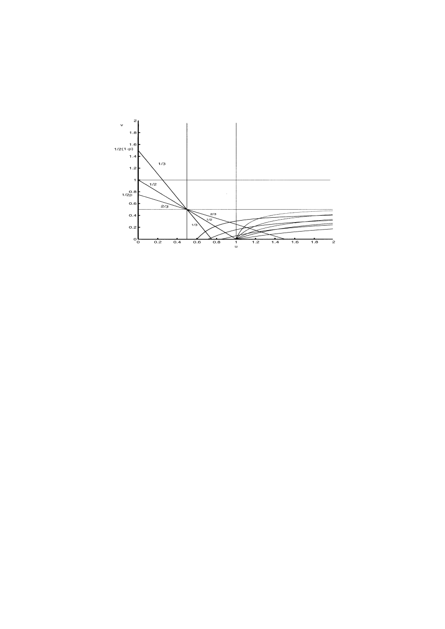
Fig. 1. The full phase diagram of TVCM with coordinates u and v. The isolines of the quantity p are straight
intervals from (1/
{2(1 − p)}, 0) to (0, 1/{2p}). The values p and 1 − p are equivalent and the corresponding
isolines are symmetric with respect to the main bisector u
= v. The acceptable part of the plane excludes the
points (u, v) such that either max(u, v) < 1/2 or min(u, v) > 1/2. Hence, the relevant part of this diagram is
made of two infinite halfstrips reducible to one another by folding along the bisector. The folded phase diagram
of TVCM corresponds to v < 0.5 < u. It shows the following curves. The isolines of 1
− p and p are straight
intervals that start at the point (1, 1) and end at the points (1/
{2p}, 0) and (1/{2(1 − p)}, 0). The isolines of D
start on the interval 1/2 < u < 1 of the u-axis and continue to the point (
∞, 0). The isolines of q
crit
start at the
point (1, 0) and continue to the point (
∞, 0). The Bernoulli binomial measure corresponds to p = 1/2 and the
canonical Cantor measure corresponds to the half line v
= 0, u > 1/2.
In this product, frequencies of wavelength > dt , to be described as “low”, contribute
µ
k
(
[0, 1]), and frequencies of wavelength < dt, to be described as “high”, contribute Ω.
5.3. The expected “partition function”
Eµ
q
(
d
i
t)
Section 6 will show that EΩ
q
need not be finite. But if it is, the limit measure µ(dt)
=
µ
k
(
dt)Ω(dt) satisfies
Eµ
q
(
dt)
= (dt)
τ (q)
+1
EΩ
q
.
The interval
[0, 1] subdivides into 1/dt intervals d
i
t
of common length dt . The sum of
the q-th moments over those intervals takes the form
Eχ (
dt)
=
Eµ
q
(
d
i
t)
= (dt)
τ (q)
EΩ
q
.
Estimation of τ (q) from a sample. It is affected by the prefactor Ω insofar as one must
estimate both τ (q) and log EΩ
q
.
Ch. 1:
Heavy Tails in Finance for Independent or Multifractal Price Increments
17
5.4. Form of the τ (q) graph
Due to conservation on the average, EM
= pu + (1 − p)v = 1/2, hence τ(1) =
− log
2
[1/2] − 1 = 0. An additional universal value is τ(0) = − log
2
(
1)
− 1 = −1. For
other values of q, τ (q) is a cap-convex continuous function satisfying τ (q) <
−1 for
q <
0.
For TVCM, a more special property is that τ (q) is asymptotically linear: assuming
u > v
, and letting q
→ ∞:
τ (q)
∼ − log
2
p
− 1 − q log u and τ(−q) ∼ − log
2
(
1
− p) − 1 + q log v.
The sign of u
− 1 affects the sign of logu, a fact that will be very important in Section 6.
Moving as little as possible beyond these properties. The very special tau function of the
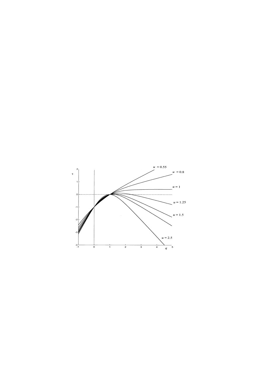
TVCM is simple but Figure 2 suffices to bring out every one of the delicate possibilities first
reported in Mandelbrot (1974a), where
−τ(q) is plotted in that little appreciated Figure 1.
Other features of τ that deserve to be mentioned. Direct proofs are tedious and the short
proofs require the multifractal formalism that will only be described in Section 11.
Fig. 2. The function τ (q) for p
= 3/4 and varying g. By arbitrary choice, the value g = 1 is assigned u = 1, from
which follows that g
= −1 is assigned to the case v = 1. Behavior of τ(q) for the value g > 0: as q → −∞, the
graph of τ (q) is asymptotically tangent to τ
= −q log
2
v
, as q
→ ∞, the graph of τ(q) is asymptotically tangent
to τ
= −q log
2
u
. Those properties are widely believed to describe the main facts about τ (q). But for TVCM they
do not. Thus, τ (q) is also tangent to τ
= qα
∗
max
and τ
= qα
∗
min
. Beyond those points of tangency, f becomes < 0.
For g > 1, that is, for u > 1, τ (q) has a maximum. Values of q beyond this maximum correspond to α
min
<
0.
Because of the capconvexity of τ (q), the equation τ (q)
= 0 may, in addition to the “universal” value q = 1,
have a root q
crit
>
1. For u > 2.5, one deals with a very different phenomenon also first described in Mandelbrot
(1974a, b). One finds that the construction of TVCM leads to a measure that degenerates to 0.

18
B.B. Mandelbrot
The quantity D(q)
= τ(q)/(q − 1). This popular expression is often called a “general-
ized dimension”, a term too vague to mean anything. D(q) is obtained by extending the
line from (q, τ ) to (1, 0) to its intercept with the line q
= 0. It plays the role of a critical
embedding codimension for the existence of a finite q-th moment. This topic cannot be
discussed here but is treated in Mandelbrot (2003).
The ratio τ (q)/q and the “accessible” values of q. Increase q from
−∞ to 0 then to
+∞. In the Bernoulli case, τ(q)/q increases from α
max
to
∞, jumps down to −∞ for
q
= 0, then increases again from −∞ to α
min
. For TVCM with p
= 1/2, the behavior
is very different. For example, let p < 1/2. As q increases from 1 to
∞, τ(q) increases
from 0 to a maximum α
∗
max
, then decreases. In a way explored in Section 10, the values of
α > α
∗
max
are not “accessible”.
5.5. Reducible and irreducible canonical multifractals
Once again, being “canonical” implies conservation on the average. When there exists a
microcanonical (conservative) variant having the same function f (α), a canonical mea-
sure can be called “reducible”. The canonical binomial is reducible because its f (α) is
shared by the Bernoulli binomial. Another example introduced in Mandelbrot (1989b) is
the “Erice” measure, in which the multiplier M is uniformly distributed on
[0, 1]. But the
TVCM with p
= 1/2 is not reducible.
In the interval
[0, 1] subdivided in the base b = 2, reducibility demands a multiplier M
whose distribution is symmetric with respect to M
= 1/2. Since u > 0, this implies u < 1.
6. When u > 1, the moment EΩ
q
diverges if q exceeds a critical exponent q
crit
satisfying τ (q)
= 0; Ω follows a power-law distribution of exponent q
crit
6.1. Divergent moments, power-law distributions and limits to the ability of moments to
determine a distribution
This section injects a concern that might have been voiced in Sections 4 and 5. The canon-
ical binomial and many other examples satisfy the following properties, which everyone
takes for granted and no one seems to think about: (a) Ω
= 1, EΩ
q
<
∞, (b) τ(q) > 0 for
all q > 0, and (c) τ (q)/q increases monotonically as q
→ ±∞.
Many presentations of fractals take those properties for granted in all cases. In fact, as
this section will show, the TVCM with u > 1 lead to the “anomalous” divergence EΩ
q
=
∞ and the “inconceivable” inequality τ(q) < 0 for q
crit
< q <
∞. Also, the monotonicity
of τ (q)/q fails for all TVCM with p
= 1/2.
Since Pareto in 1897, infinite moments have been known to characterize the power-law
distributions of the form Pr
{X > x} = x
−q
crit
. But in the case of TVCM and other canonical
multifractals, the complicating factor L(x) is absent. One finds that when u > 1, the overall
measure Ω follows a power law of exponent q
crit
determined by τ (q).

Ch. 1:
Heavy Tails in Finance for Independent or Multifractal Price Increments
19
6.2. Discussion
The power-law “anomalies” have very concrete consequences deduced in Mandelbrot
(1997) and discussed, for example, in Mandelbrot (2001c).
But does all this make sense? After all, τ (q) and EΩ
q
are given by simple formulas and
are finite for all parameters. The fact that those values cannot actually be observed raises a
question. Are high moments lost by being unobservable? In fact, they are “latent” but can
be made “actual” by a process is indeed provided by the process of “embedding” studied
elsewhere.
An additional comment is useful. The fact that high moments are non-observable does
not express a deficiency of TVCM but a limitation of the notion of moment. Features
ordinarily expressed by moments must be expressed by other means.
6.3. An important apparent “anomaly”: in a TVCM, the q-th moment of Ω may diverge
Let us elaborate. From long past experience, physicists’ and statisticians’ natural impulse
is to define and manipulate moments without envisioning or voicing the possibility of their
being infinite. This lack of concern cannot extend to multifractals. The distribution of the
TVCM within a dyadic interval introduces an additional critical exponent q
crit
that satis-
fies q
crit
>
1. When 1 < q
crit
<
∞, which is a stronger requirement that D > 0, the q-th
moment of µ(dt) diverges for q > q
crit
.
A stronger result holds: the TVCM cascade generates a measure whose distribution fol-
lows the power law of exponent q
crit
.
Comment. The heuristic approach to non-random multifractals fails to extend to random
ones, in particular, it fails to allow q
crit
<
∞. This makes it incomplete from the viewpoint
of finance and several other important applications.
The finite q
crit
has been around since Mandelbrot (1974a, b) (where it is denoted by α)
and triggered a substantial literature in mathematics. But it is linked with events so extra-
ordinarily unlikely as to appear incapable of having any perceptible effect on the gener-
ated measure. The applications continue to neglect it, perhaps because it is ill-understood.
A central goal of TVCM is to make this concept well-understood and widely adopted.
6.4. An important role of τ (q): if q > 1 the q-th moment of Ω is finite if, and only if,
τ (q) >
0; the same holds for µ(dt) whenever dt is a dyadic interval
By definition, after k levels of iteration, the following symbolic equality relates indepen-
dent realizations of M and µ. That is, it does not link random variables but distributions
µ
k
[0, 1]
= Mµ
k
−1
[0, 1]
+ Mµ
k
−1
[0, 1]
.
Conservation on the average is expressed by the identity Eµ
k
−1
(
[0, 1]) = 1. In addition,
we have the following recursion relative to the second moment.
Eµ
2
[0, 1]
= 2EM
2
Eµ
2
k
−1
[0, 1]
+ 2EM
2
Eµ
k
−1
[0, 1]
2
.

20
B.B. Mandelbrot
The second term to the right reduces to 1/2. Now let k
→ ∞. The necessary and suffi-
cient condition for the variance of µ
k
(
[0, 1]) to converge to a finite limit is
2
EM
2
<
1
in other words
τ (
2)
= − log
2
EM
2
− 1 > 0.
When such is the case, Kahane and Peyrière (1976) gave a mathematically rigorous
proof that there exists a limit measure µ(
[0, 1]) satisfying the formal expression
Eµ
2
[0, 1]
=
1
2(1
− 2
τ (
2)
)
.
Higher integer moments satisfy analogous recursion relations. That is, knowing that all
moments of order up to q
− 1 are finite, the moment of order q is finite if and only if
τ (q) >
0.
The moments of non-integer order q are more delicate to handle, but they too are finite
if, and only if, τ (q) > 0.
6.5. Definition of q
crit
; proof that in the case of TVCM q
crit
is finite if, and only if, u > 1
Section 5.4 noted that the graph of τ (q) is always cap-convex and for large q > 0,
τ (q)
∼ − log
2
pu
q
+ −1 ∼ − log
2
p
− 1 − q log
2
u.
The dependence of τ (q) on q is ruled by the sign of u
− 1, as follows.
• The case when u < 1, hence α
min
>
0. In this case, τ (q) is monotone increasing and
τ (q) >
0 for q > 1. This behavior is exemplified by the Bernoulli binomial.
• The case when u > 1, hence α
min
<
0. In this case, one has τ (q) < 0 for large q. In ad-
dition to the root q
= 1, the equation τ(q) = 1 has a second root that is denoted by q
crit
.
Comment. In terms of the function f (α) graphed on Figure 3, the values 1 and q
crit
are
the slopes of the two tangents drawn to f (α) from the origin (0, 0).
Within the class of equivalence of any p and 1
− p; the parameter g can be “tuned” so
that q
crit
begins by being > 1 then converges to 1; if so, it is seen that D converges to 0.
• Therefore, the conditions q
crit
= 1 and D = 0 describe the same “anomaly”.
In Figure 1, isolines of q
crit
are drawn for q
crit
= 1, 2, 3, and 4. When q = 1 is the only
root, it is convenient to say that q
crit
= ∞. This isoset q
crit
= ∞ is made of the half-line
{v = 1/2 and u > 1/2} and of the square {0 < v < 1/2, 1/2 < u < 1}.
6.6. The exponent q
crit
can be considered as a macroscopic variable of the generating
process
Any set of two parameters that fully describes a TVCM can be called “microscopic”. All
the quantities that are directly observable and can be called macroscopic are functions of
those two parameters.
Ch. 1:
Heavy Tails in Finance for Independent or Multifractal Price Increments
21
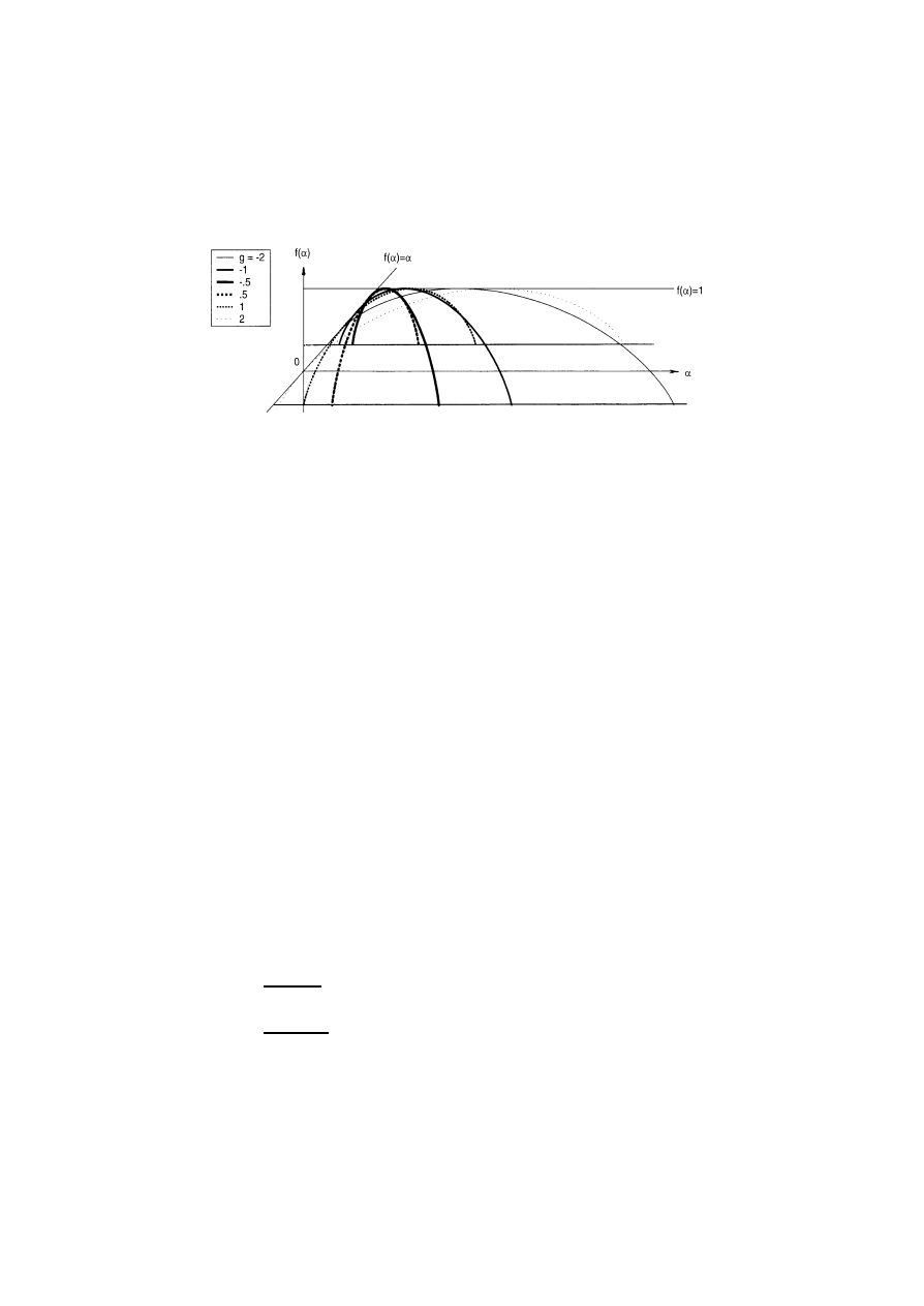
Fig. 3. The functions f (α) for p
= 3/4 and varying g. All those graphs are linked by horizontal reductions or
dilations followed by translation and further self-affinity. It is widely anticipated that f (α) > 0 holds in all cases,
but for the TVCM this anticipation fails, as shown in this figure. For g > 0 (resp., g < 0) the left endpoint of f (α)
(resp., the right endpoint) satisfies f (α) < 0 and the other endpoint, f (α) > 0.
For the general canonical multifractal, a full specification requires a far larger number
of microscopic quantities but the same number of macroscopic ones. Some of the latter
characterize each sample, but others, for example q
crit
,
characterize the population.
7. The quantity α: the original Hölder exponent and beyond
The multiplicative cascades – common to the Bernoulli and canonical binomials and
TVCM – involve successive multiplications. An immediate consequence is that both the
basic µ(dt) and its probability are most intrinsically viewed through their logarithms.
A less obvious fact is that a normalizing factor 1/ log(dt) is appropriate in each case.
An even less obvious fact is that the normalizations log µ/ log dt and log P / log dt are of
far broader usefulness in the study of multifractals. The exact extend of their domain of
usefulness is beyond the goal of this chapter, but we keep some special cases that can be
treated fully by elementary arguments.
7.1. The Bernoulli binomial case and two forms of the Hölder exponent: coarse-grained
(or coarse) and fine-grained
Recall that due to conservation, the measure in an interval of length dt
= 2
−k
is the same
after k stages and in the limit, namely, µ(dt)
= µ
k
(
dt). As a result, the coarse-grained
Hölder exponent can be defined in either of two ways,
α(
dt)
=
log µ(dt)
log(dt)
and
˜α(dt) =
log µ
k
(
dt)
log(dt)
.

22
B.B. Mandelbrot
The distinction is empty in the Bernoulli case but prove prove essential for the TVCM.
In terms of the relative frequencies ϕ
0
and ϕ
1
defined in Section 2.1,
α(
dt)
= ˜α(dt) = α(ϕ
0
, ϕ
1
)
= −ϕ
0
log
2
u
− ϕ
1
log
2
v
= −ϕ
0
(
log
2
u
− log
2
v)
− log v.
Since u > v, one has 0 < α
min
= − log
2
u
α = ˜α α
max
= − log
2
v <
∞. In particu-
lar, α > 0, hence
˜α > 0. As dt → 0, so does µ(dt), and a formal inversion of the definition
of α yields
µ(
dt)
= (dt)
α
.
This inversion reveals an old mathematical pedigree. Redefine ϕ
0
and ϕ
1
from denoting
the finite frequencies of 0 and 1 in an interval, into denoting the limit frequencies at an
instant t . The instant t is the limit of an infinite sequence of approximating intervals of
duration 2
−k
. The function µ(
[0, t]) is non-differentiable because lim
dt
→0
µ(
dt)/dt is not
defined and cannot serve to define the local density of µ at the instant dt .
The need for alternative measures of roughness of a singularity expression first arose
around 1870 in mathematical esoterica due to L. Hölder. In fractal/multifractal geometry
this expression merged with a very concrete exponent due to H.E. Hurst and is continually
being generalized. It follows that for the Bernoulli binomial measure, it is legitimate to
interpret the coarse αs as finite-difference surrogates of the local (infinitesimal) Hölder
exponents.
7.2. In the general TVCM measure, α
= ˜α, and the link between “α” and the Hölder
exponent breaks down; one consequence is that the “doubly anomalous”
inequalities α
min
<
0, hence
˜α < 0, are not excluded
A Hölder (Hurst) exponent is necessarily positive. Hence negative
˜αs cannot be interpreted
as Hölder exponents. Let us describe the heuristic argument that leads to this paradox and
then show that
˜α < 0 is a serious “anomaly”: it shows that the link between “some kind
of α” and the Hölder exponent requires a searching look. The resolution of the paradox is
very subtle and is associated with the finite q
crit
introduced in Section 6.5.
Once again, except in the Bernoulli case, Ω
= 1 and µ(dt) = µ
k
(
dt)Ω(dt), hence
α(
dt)
= ˜α(dt) +
log Ω(dt)
log dt.
In the limit dt
→ 0 the factor log = Ω/ log(dt) tends to 0, hence it seems that α = ˜α.
Assume u > 1, hence α
min
<
0 and consider an interval where
˜α(dt) < 0. The formal
equality
“µ
k
(
dt)
= (dt)
˜α
”

Ch. 1:
Heavy Tails in Finance for Independent or Multifractal Price Increments
23
seems to hold and to imply that “the” mass in an interval increases as the interval length
→ 0. On casual inspection, this is absurd. On careful inspection, it is not – simply because
the variable dt
= 2
−k
and the function µ
k
(
dt) both depend on k. For example, consider the
point t for which ϕ
0
= 1. Around this point, one has µ
k
= uµ
k
−1
> µ
k
−1
. This inequality
is not paradoxical.
Furthermore, Section 8 shows that the theory of the multiplicative measures introduces
˜α intrinsically and inevitably and allows ˜α < 0.
Those seemingly contradictory properties will be reexamined in Section 9. Values of
µ(
dt) will be seen to have a positive probability but one so minute that they can never be
observed in the way α > 0 are observed. But they affect the distribution of the variable Ω
examined in Section 4, therefore are observed indirectly.
8. The full function f (α) and the function ρ(α)
8.1. The Bernoulli binomial measure: definition and derivation of the box dimension
function f (α)
The number of intervals of denumerator 2
−k
leading to ϕ
0
and ϕ
1
is N (k, ϕ
0
, ϕ
1
)
=
k
!/(kϕ
0
)
!(kϕ
1
)
!, and dt is the reduction ratio r from [0, 1] to an interval of duration dt.
Therefore, the expression
f (k, ϕ
0
, ϕ
1
)
= −
log N (k, ϕ
0
, ϕ
1
)
log(dt)
= −
log
[k!/(kϕ
0
)
!(kϕ
1
)
!]
log(dt)
is of the form f (k, ϕ
0
, ϕ
1
)
= − logN/ log r. Fractal geometry calls this the “box similar-
ity dimension” of a set. This is one of several forms taken by fractal dimension. More
precisely, since the boxes belong to a grid, it is a grid fractal dimension.
The dimension function f (α). For large k, the leading term in the Stirling approximation
of the factorial yields
lim
k
→∞
f (k, ϕ
0
, ϕ
1
)
= f (ϕ
0
, ϕ
1
)
= −ϕ
0
log
2
ϕ
0
− ϕ
1
log
2
ϕ
1
.
8.2. The “entropy ogive” function f (α); the role of statistical thermodynamics in
multifractals and the contrast between equipartition and concentration
Eliminate ϕ
0
and ϕ
1
between the functions f and α
= −ϕ
0
log u
− ϕ
1
log v. This yields in
parametric form a function, f (α). Note that 0
f (α) min{α, 1}. Equality to the right is
achieved when ϕ
0
= u. The value α where f = α is very important and will be discussed
in Section 9. In terms of the reduced variable ϕ
0
= (α − α
min
)/(α
max
− α
min
)
, the function
f (α)
becomes the “ogive”
˜
f (ϕ
0
)
= −ϕ
0
log
2
ϕ
0
− (1 − ϕ
0
)
log
2
(
1
− ϕ
0
).

24
B.B. Mandelbrot
This ˜
f (ϕ
0
)
can be called a universal function. The f (α) corresponding to fixed p and
varying g are affine transforms of ˜
f (ϕ
0
)
, therefore of one another. The ogive function ˜
f
first arose in thermodynamics as an entropy and in 1948 (with Shannon) entered com-
munication theory as an information. Its occurrence here is the first of several roles the
formalism of thermodynamics plays in the theory of multifractals.
An essential but paradoxical feature. Equilibrium thermodynamics is a study of various
forms of near-equality, for example postulates the equipartition of states on a surface in
phase space or of energy among modes. In sharp contrast, multifractals are characterized
by extreme inequality between the measures in different intervals of common duration dt .
Upon more careful examination, the paradox dissolves by being turned around: the main
tools of thermodynamics can handle phenomena well beyond their original scope.
8.3. The Bernoulli binomial measure, continued: definition and derivation of a function
ρ(α)
= f (α) − 1 that originates as a rescaled logarithm of a probability
The function f (α) never fully specifies the measure. For example, it does not distinguish
between the Bernoulli, shuffled and canonical binomials. The function f (α) can be gener-
alized by being deduced from a function ρ(α)
= f (α)−1 that will now be defined. Instead
of dimensions, that deduction relies on probabilities. In the Bernoulli case, the derivation
of ρ is a minute variant of the argument in Section 8.1, but, contrary to the definition of f ,
the definition of ρ easily extends to TVCM and other random multifractals.
In the Bernoulli binomial case, the probability of hitting an interval leading to ϕ
0
and ϕ
1
is simply P (k, ϕ
0
, ϕ )
= N(k, ϕ
0
, ϕ
1
)
2
−k
= k!/(kϕ
0
)
!(kϕ
1
)
!2
−k
. Consider the expression
ρ(k, ϕ
0
, ϕ
1
)
= −
log
[P (k, ϕ
0
, ϕ
1
)
]
log(dt)
,
which is a rescaled but not averaged form of entropy. For large k, Stirling yields
lim
k
→∞
ρ(k, ϕ
0
, ϕ
1
)
= ρ(ϕ
0
, ϕ
1
)
= −ϕ
0
log
2
ϕ
0
− ϕ
1
log
2
ϕ
1
− 1
= f (α) − 1.
8.4. Generalization of ρ(α) to the case of TVCM; the definition of f (α) as ρ(α)
+ 1 is
indirect but significant because it allows the generalized f to be negative
Comparing the arguments in Sections 8.1 and 8.2 link the concepts of fractal dimension
and of minus log (probability). However, when f (α) is reported through f (α)
= ρ(α) + 1,
the latter is not a mysterious “spectrum of singularities”. It is simply the peculiar but proper
way a probability distribution must be handled in the case of multifractal measures. More-
over, there is a major a priori difference exploited in Section 10. Minus log (probability)
is not subjected to any bound. To the contrary, every one of the traditional definitions of
fractal dimension (including Hausdorff–Besicovitch or Minkowski–Bouligand) necessar-
ily yields a positive value.
Ch. 1:
Heavy Tails in Finance for Independent or Multifractal Price Increments
25
The point is that the dimension argument in Section 8.1 does not carry over to TVCM,
but the probability argument does carry over as follows. The probability of hitting an in-
terval leading to ϕ
0
and ϕ
1
now changes to P (k, ϕ
0
, ϕ
1
)
= p(ϕ
0
k)
!/(kϕ
0
)
!(kϕ
1
)
! One can
now form the expression
ρ(k, ϕ
0
, ϕ
1
)
= −
log
[P (k, ϕ
0
, ϕ
1
)
]
log(dt)
.
Stirling now yields
ρ(ϕ
0
, ϕ
1
)
= lim
k
→∞
ρ(k, ϕ
0
, ϕ
1
)
= {−ϕ
0
log
2
ϕ
0
− ϕ
1
log
2
ϕ
1
} +
ϕ
0
log
2
p
+ ϕ
1
log
2
(
1
− p)
.
In this sum of two terms marked by braces, we know that the first one transforms (by
horizontal stretching and translation) into the entropy ogive. The second is a linear function
of ϕ, namely ϕ
0
[log
2
p
− log
2
(
1
− p)] + log
2
(
1
− p). It transforms the entropy ogive by
an affinity in which the line joining the two support endpoints changes from horizontal to
inclined. The overall affinity solely depends on p, but ϕ
0
depends explicitly on u and v.
This affinity extends to all values of p. Another property familiar from the binomial
extends to all values of p. For all u and v, the graphs of ρ(α), hence of f (α) have a
vertical slope for q
= ±∞.
Alternatively, ρ(ϕ
0
, ϕ
1
)
= −ϕ
0
log
2
[ϕ
0
/p
] − ϕ
1
log
2
[ϕ
1
/(
1
− p)].
8.5. Comments in terms of probability theory
Roughly speaking, the measure µ is a product of random variables, while the limit
theorems of probability theory are concerned with sums. The definition of α as
log µ(dt)/ log(dt) replaces a product of random variables M by a weighted sum of ran-
dom variables of the form log M. Let us now go through this argument step by step in
greater rigor and generality. One needs a cumbersome restatement of α
k
(
dt).
The low frequency factor of µ
k
(
dt) and the random variable H
low
. Consider once again
a dyadic cell of length 2
−k
that starts at t
= 0.β
1
β
2
. . . β
k
. The first k stages of the cascade
can be called of low frequency because they involve multipliers that are constant over
dyadic intervals of length dt
= 2
−
k
or longer. These stages yield
µ
k
(
dt)
= M(β
1
)M(β
1
, β
2
)
· · ·M(β
1
, . . . , β
k
)
=
M.
We transform µ
k
(
dt) into the low frequency random variable
H
low
=
log
[µ
k
(
dt)
]
log(dt)
=
1
k
− log
2
M(β
1
)
− log
2
M(β
1
, β
2
)
− · · ·
.

26
B.B. Mandelbrot
We saw in Section 4.5 that the first few values of M largely determine the distribution
of Ω. But the last expression involves an operation of averaging in which the first terms
contributing to µ(dt) are asymptotically washed out.
8.6. Distinction between “center” and “tail” theorems in probability
The quantity
˜α
k
(
dt)
= ϕ
0
log
2
u
− ϕ
1
log
2
v
is the average of a sum of variables
− logM;
but why is its distribution is not Gaussian and the graph of ρ(α) is an entropy ogive rather
than a parabola? Why is this so? The law of large numbers tells us that
˜α
k
(
dt) almost
surely converges to its expectation which tells us very little. A tempting heuristic argu-
ment continues as follows. The central limit theorem is believed to ensure that for small
dt, H
low
(
dt) becomes Gaussian, therefore the graph of log p(dt) should be expected to be
a parabola. This being granted, why is it that the Stirling approximation yields an entropy
ogive – not a parabola?
In fact, there is no paradox of any kind. While the central limit theorem is indeed central
to probability theory, all it asserts in this context is that, asymptotically, the Gaussian rules
the center of the distribution, its “bell”. Renormalizations reduce this center to the imme-
diate neighborhood of the top of the ρ(α) graph and the central limit theorem is correct in
asserting that the top of the entropy ogive is locally parabolic. But in the present context
this information is of little significance. We need instead an alternative that is only con-
cerned with the tail behavior which it ought to blow up. For this and many other reasons,
it would be an excellent idea to speak of center, not central limit theorem. The tail limit
theorem is due to H. Cramer and asserts that the tail consisting in the bulk of the graph is
not a parabola but an entropy ogive.
8.7. The reason for the anomalous inequalities f (α) < 0 and α < 0 is that, by the
definition of a random variable µ(dt), the sample size is bounded and is prescribed
intrinsically; the notion of supersampling
The inequality ρ(α) <
−1 characterizes events whose probability is extraordinarily small.
The finding that this inequality plays a significant role was not anticipated, remains difficult
to understand and appreciate, and demands comment.
The common response is that even extremely low probability events are captured if one
simply takes a sufficiently long sample of independent values. But this is impossible, even
if one forgets that, in the present uncommon context, the values are extremely far from
being statistically independent. Indeed, the choice the duration dt
= 2
−k
has two effects.
Not only does it fix the distribution of µ(dt), but it also sets the sample size at the value
N
= 1/dt = 2
k
. Roughly speaking, a sample of size N can only reveal values having a
probability greater than 1/N , which means ρ(α) >
−1.
In summary, it is true that decreasing dt to 2
−k−1
increases the sample size. But it
also changes the distribution and does so in such a way that the bound ρ
= −1 remains
untouched.

Ch. 1:
Heavy Tails in Finance for Independent or Multifractal Price Increments
27
This bound excludes ∂u items of information that correspond to f (α) < 0 (for example,
the value of q
crit
when finite). Those items remain hidden and latent in the sense that they
cannot be inferred from one sample of values of µ(dt). Ways of revealing those values, su-
persampling and embedding, are examined in Mandelbrot (1989b, 1995) and forthcoming
Mandelbrot (2003).
Figure 3 shows, for p
= 3/4, how the graph of f (α) depends on g.
8.8. Excluding the Bernoulli case p
= 1/2, TVCM faces either one of two major
“anomalies”: for p >
−1/2, one has f (α
min
)
= 1 + log
2
p >
0 and
f (α
max
)
= 1 + log
2
(
1
− p) < 0; for p < 1/2, the opposite signs hold
The fact that the values of ρ(α
min
)
= f (α
min
)
− 1 and ρ(α
max
)
= f (α
max
)
− 1 are loga-
rithms of probabilities confirms and extends the definition of p(α)
= f (α) − 1 as a limit
rescaled probability. Here, those endpoint values of f (α) are independent of g and the
affinity that deduces them from the entropy ogive (with ends on the horizontal axis) char-
acterizes the class of equivalence of p and 1
−p. If, and only if, p = 1/2 and u+v = 1, that
is, in the familiar Bernoulli binomial case, one has ρ(α
min
)
= ρ(α
max
)
= log
2
(
1/2)
= −1
hence f (α
min
)
= f (α
max
)
= 0. When u + v = 1, one of the endpoints satisfies f > 0 and
the other satisfies f < 0. Sections 8.9 and 10 shall examine the sharply differing conse-
quences of those inequalities.
8.9. The “minor anomalies” f (α
max
) >
0 or f (α
min
) >
0 lead to sample function with a
clear “ceiling” or “floor”
Suppose that f (α
min
)
= 0 and f (α
max
)
= 0, as is the case for p = 1/2. Then, using terms
often applied to the printed page – but after it has been turned 90
◦
to the side – the sample
functions are “non-justified” or “ragged” for both high and low values. That is, the values
tend to be unequal; one is clearly larger than all others, a second is clearly the second
largest, etc.
To the contrary, TVCM with p
= 1/2 yield either f (α
max
) >
0 or f (α
min
) >
0. Sample
functions have a conspicuous “ceiling” (resp., a “floor”). That is, a largest (resp., smallest)
value is attained repeatedly for values of t belonging to a set of positive dimension. To
use the printers’ vocabulary, when one side is “ragged” the other is “justified”. On visual
inspection of the data, the ceiling is always visible; the floor merges with the time axis,
except when one plots log
[µ(dt)].
9. The fractal dimension D
= τ
(
1)
= 2[−pu log
2
u
− (1 − p)v log
2
v
] and
multifractal concentration
The function f (α) satisfies f (α)
α, with equality f (α) = α when α = D = τ(1). From
the value of α
= D follows one of the most important properties of multifractals. Mandel-
brot (2001d) proposed to call it “multifractal concentration”. This section will first examine
its opposite, which is asymptotic negligibility.

28
B.B. Mandelbrot
9.1. In the Bernoulli binomial measures weak asymptotic negligibility holds but strong
asymptotic negligibility fails
Recall that during construction, the total binomial measure of
[0, 1] remains constant and
equal to 1. But the first few stages of construction make its distribution become very un-
equal and a few values that stand out as sharp spikes. After k stages, the maximum measure
is u
k
, which is far larger than the minimum measure v
k
. From the relations
2
−k
= dt, 2
k
= N, − log
2
u
= α
min
<
1,
and
− log
2
v
= α
min
>
1,
it follows that
u
k
= b
(
− log
b
u)(
−k)
= (dt)
α
min
= N
−α
min
.
In words: even the maximum u
k
tends to 0. This is a weak form of asymptotic negligi-
bility following a power-law.
The preceding result holds for every multifractal for which there is an α
min
>
0 that
plays the same role as in the binomial case. (In more general multifractals the same role is
held by some α
∗
min
>
max
{α
min
,
0
}.)
Similarly, the total contribution of any fixed number of largest spikes is asymptotically
negligible.
9.2. For the Bernoulli or canonical binomials, the equation f (α)
= α has one and only
one solution; that solution satisfies D > 0 and is the fractal dimension of the
“carrier” of the measure
We now proceed to the total contribution of a number of spikes that is no longer fixed but
increases with N . In the simplest of all possible worlds, many spikes would have been more
or less equal to the largest, and the sum of all the other spikes would have been negligible.
If so, the sum of N
α
min
spikes would have been of the order of N
α
min
N
−α
min
= 1.
While the world is actually more complicated there is an element of orderliness. The
equality ϕ
0
= u is achieved for α = f (α) = −u logu − v logv = D. For finite but large k,
it follows that
µ(k, ϕ
0
, ϕ
1
)
∼ 2
−kα
= 2
−kD
and
N (k
1
ϕ
0
, ϕ
1
)
∼ 2
kf (α)
= 2
kD
.
Hence,
µ(k
1
ϕ
0
, ϕ
1
)N (k
1
ϕ
0
ϕ
1
)
is approximately equal to 1.
Actually, this product is necessarily
1 but the difference tends to 0 as k → ∞. That
is, an increasingly overwhelming bulk of the measure tends to “concentrate” in the cells
where α
= D. The remainder is small, but in the theory of multifractals even very small
remainders are extremely significant for some purposes.

Ch. 1:
Heavy Tails in Finance for Independent or Multifractal Price Increments
29
9.3. The notion of “multifractal concentration”
A key feature of multifractals is a subtle interaction between number and size that is elabo-
rated upon in Mandelbrot (2001d). Section 9.2 showed that the contributions that are large
are too few to matter. The small contributions are very numerous, but so extremely small
that their total contribution is negligible as well. The bulk of the measure is found in a
rather inconspicuous intermediate range one can call “mass carrying”. Since D > α
min
, the
N
D
spikes of size N
−D
are far smaller than the largest one. Separately, each is asymp-
totically negligible. But their number N
D
is exactly large enough to insure that their total
contribution is nearly equal to the overall measure 1. When a sample is plotted, this range
does not stand out but it makes a perfect match between size and frequency.
Practically, the number of visible peaks is so small compared to N
D
that a combination
of the peaks and the intermediate range is still of the order of N
D
. The combined range
has the advantage of simplicity, since it includes the N
D
largest values. Note that the peaks
tend to be located in the midst of stretches of values of intermediate size.
9.4. The case of TVCM with p < 1/2, allows D to be positive, negative, or zero
Using the alternative expression for f (α) given in Section 8.4, the identity f (α)
= α de-
mands the equality of the two expressions
f (α)
= −ϕ
0
log
2
ϕ
0
p
− ϕ
1
log
2
ϕ
1
1
− p
and
α
= −ϕ
0
log
2
u
− ϕ
1
log
2
v.
The solution is, obviously, ϕ
0
= pu and ϕ
1
= (1 − p)v. The sum ϕ
1
+ ϕ
1
is 1, as it must.
Hence, D
= −pu log
2
u
− (1 − p)v log
2
v
, as announced. The novelty is that TVCM allow
D >
0, D
= 0, and D < 0.
Familiar role of D under the inequality D > 0. Mandelbrot (1974a, b) obtained the
following criterion, which has become widely known and includes the TVCM case. When
positive, D is the fractal dimension of the “set that supports” the measure. Figure 1 shows
isolines of D for D
= 0, 1/4, 1/2, and 3/4. The isoline for D = 1 is made of the interval
{u = 1, 0 < v < 1} and the half-line {v = 1, u 1}. The key result is that, contrary to the
Bernoulli binomial case, the half line 1 < q <
∞ subdivides into up to three subranges of
values.
Largely unfamiliar consequence of the inequality D < 0. For all non-random multifrac-
tals, τ
(1) > 0. A casual acquaintance with multifractals takes for granted that this is not
changed by randomness. But Mandelbrot (1974a, b) also allows for an alternative possi-
bility, which has so far remained little known. The example of TVCM shows that, in a
canonical case, the formally evaluated D can be negative. In the example of TVCM, D is
negative when the point (u, v) falls in a domain to the bottom right of the folded phase
diagram in Figure 1. The consequences of D < 0 are drastic: the multifractal reduces to 0
almost surely and is called degenerate.
A classical “pathological limit” as metaphor. This limit behavior of the distribution of
µ
seems incompatible with the fact that Eµ
= 1 by definition. But in fact, no contradiction

30
B.B. Mandelbrot
is observed. A convincing idea of the distribution is provided for each p, by the behavior
of the g
→ ∞ limit of the weights u
g
2
τ (g)
and v
g
2
τ (g)
. This recalls a classical counterex-
ample of analysis, namely, the behavior for k
→ ∞ of the variable P
k
defined as follows:
P
k
= k with the probability 1/k and P
k
= 0 with the probability 1 − 1/k. For finite k, one
has EP
k
= 1. But in the limit k → ∞, P
∞
= 0, hence EP
∞
= 0, so that in the limit the
expectation drops discontinuously from 1 to 0. In practice, the preasymptotic measure is
extremely small with a high probability and huge with a tiny probability.
The condition D
= 0. It defines the threshold of degeneracy.
10. A noteworthy and unexpected separation of roles, between the “dimension
spectrum” and the total mass Ω; the former is ruled by the accessible α for
which f (α) > 0, the latter, by the inaccessible α for which f (α) < 0
Brought together, Sections 4, 7, 8, and 9 imply, in plain words, that what you do not nec-
essarily see may affect you significantly. This section serves to underline that the notion
of canonical multifractal is very subtle and deserves to be well-understood and further
discussed.
10.1. Definitions of the “accessible ranges” of the variables: qs from q
∗
min
to q
∗
max
and αs
from α
∗
min
to α
∗
max
; the accessible functions τ
∗
(q) and f
∗
(α)
Mandelbrot (1995) worked to introduce to the function f
∗
(α)
= max{0, f (α)}. That is,
• In the interval [α
∗
min
, α
∗
max
] where f (α) > 0, f
∗
(α)
= f (α);
• When f (α) 0, f
∗
(α)
= 0.
The graph of f
∗
(α)
is identical to that of f (α) except that the “tails” with f < 0 are
truncated so that f
∗
>
0. In terms of τ (q), the equality f (α)
= 0 corresponds to lines that
are tangent to the graph of τ (q) and also go through (0, 0). In the most general case, those
lines’ slopes are α
∗
min
and α
∗
max
and the points of contact are denoted by q
∗
max
(satisfying
>
0) and q
∗
min
(satisfying <0). Therefore, the function f
∗
(α)
corresponds to the following
truncated function τ
∗
(q)
.
• When q < q
∗
min
, τ
∗
(q)
= α
∗
max
q
;
• When q
∗
min
< q < q
∗
max
, τ
∗
(q)
= τ(q);
• When q > q
∗
max
, τ
∗
(q)
= α
∗
min
q
.
In other words, the graph of τ
∗
is identical to that of τ except that beyond q
∗
max
or q
∗
min
it follows the tangents that go through the origins. Therefore it is straight.
For the TVCM, one has either α
∗
max
= α
max
with q
∗
min
= −∞, or α
∗
min
= α
min
with
q
∗
max
= ∞.
10.2. A confrontation
Section 4 noted that the largest values of Ω(
[0, 1]) are generated when a sample cascade
begins with a few large values. Section 7 noted that the value of Ω(
[0, 1]) – irrespective of

Ch. 1:
Heavy Tails in Finance for Independent or Multifractal Price Increments
31
size – ceases, for k
→ ∞, to have any impact on α. Section 8 noted that, again for k → ∞,
values of α such that f (α) < 0 have a vanishing probability of being observed. Section 9.1
followed up by defining the accessible function f (α). Section 9 returned to large values of
Ω(
[0, 1]) and noted their association with q
crit
<
∞. The values of α they involve satisfy
α <
0, hence a fortiori f (α) < 0. Those values do not occur in multifractal decomposition,
yet they are extremely important.
10.3. The simplest cases where f (α) > 0 for all α, as exemplified by the canonical
binomial
Here, the large values of Ω are ruled by the left-most part of the graph of f (α). That is, the
same graph controls those large values and the distribution of Ω(
[0, 1]) among the 1/dt
intervals of length dt .
10.4. The extreme case where f (α) < 0 and α < 0 both occur, as exemplified by TVCM
when u > 1
Due to the inequality f (α) < α, the graph of f (α) never intersects the quadrant where
α <
0 and f > 0. The key unexpected fact is that the portions of f (α) within other quad-
rants play more or less separate roles. In the TVCM case, those quadrants are parts of one
(analytically simple) function. But in general they are nearly independent of each other.
The function f (α) was defined as having a graph that lies in the non-anomalous quadrant
α >
0 and f > 0. This f determines completely the multifractal decomposition of our
TVCM measure, in particular, the dimension D and the exponents q
∗
min
, q
∗
max
, α
∗
min
and
α
∗
max
.
To the contrary, q
crit
is entirely determined by the doubly anomalous left tail located in
the quadrant characterized by f (α) < 0 and α < 0. A priori, it was quite unexpected that
this quadrant should exist and play any role, least of all a central role, in the theory of
multifractals. But in fact, q
crit
has a major effect on the distribution, hence the value of the
total measure in an interval.
10.5. The intermediate case where α
min
>
0 but f (α) < 0 for some values of α
When p < 1/2, but u < 1 so that q
crit
= ∞ and all moments are finite, large values of
µ
have a much lower probability than when u > 1. As always, however, their probability
distribution continues to be determined by the left tail of the probability graph where f < 0.
11. A broad form of the multifractal formalism that allows α < 0 and f (α) < 0
The collection of rules that relate τ (q) to f (α) is called “multifractal formalism”. TVCM
was specifically designed to understand multifractals directly, thus avoiding all formalism.

32
B.B. Mandelbrot
However, general random multifractals more than TVCM demand their own broad multi-
fractal formalism. Once again, the most widely known form of the multifractal formalism
does not allow randomness and yields f (α) > 0, but the broad formalism first introduced
in Mandelbrot (1974a, b) concerns a generalized function for which f (α) < 0 is allowed.
11.1. The broad “multifractal formalism” confirms the form of f (α) and allows
f (α) <
0 for some α
Through a point on the graph of coordinates q and τ (q), draw the tangent to that graph.
Under wide conditions, the tangent’s slope is α(q) and its intercept by the ordinate axis is
−f (q). Thus
α(q)
=
dτ (q)
dq
and
− f (q) = τ(q) − q
dτ (q)
dq
.
Through the quantities α(q) and f (q), a function f (α) is defined by using q as parame-
ter.
The slope f
(α)
is the inverse of the function α(q). The tangent of slope f
(α)
inter-
sects the line α
= 0 at the point of ordinate −τ(q). The D(q) tangent’s equation being
−τ(q) + qα, its intersection with the bisector satisfies the condition −τ + q = α, hence
D
= τ(q)/(q − 1). This is the critical embedding dimension discussed in Section 5.4.
11.2. The Legendre and inverse Legendre transforms and the thermodynamical analogy
The transforms that replace q and τ (q) by α and f (α), or conversely, are due to Legendre.
They play a central role in thermodynamics, as does already the argument that yielded
f (α)
and ρ(α) in the original formalism introduced in Mandelbrot (1974a, b).
Acknowledgments
The figures in this chapter were prepared by Evgenyi Vilenkin, Yale class of 2003.
References
Chernoff, H., 1952. A measure of asymptotic efficiency for tests of a hypothesis based on the sum of observations.
The Annals of Mathematical Statistics 23, 493–507.
Cootner, P.H. (Ed.), 1964. The Random Character of Stock Market Prices. MIT Press, Cambridge, MA.
Daniels, H.E., 1954. Saddlepoint approximations in statistics. The Annals of Mathematical Statistics 25, 631–649.
Durrett, R., Liggett, T.M., 1983. Fixed points of the smoothing transformation. Zeitschrift für Wahrscheinlich-
keitstheorie 64, 275–301.
Frisch, U., Parisi, G., 1985. Fully developed turbulence and intermittency. In: Ghil, M. (Ed.), Turbulence and
Predictability in Geophysical Fluid Dynamics and Climate Dynamics, North-Holland, pp. 84–86. Excepted in
Mandelbrot (1999a).

Ch. 1:
Heavy Tails in Finance for Independent or Multifractal Price Increments
33
Halsey, T.C., Jensen, M.H., Kadanoff, L.P., Procaccia, I., Shraiman, B.I., 1986. Fractal measures and their singu-
larities: the characterization of strange sets. Physical Review A 33, 1141–1151.
Hentschel, H.G.E., Procaccia, I., 1983. The infinite number of generalized dimensions of fractals and strange
attractors. Physica (Utrecht) 8D, 435–444.
Kahane, J. P., Peyrière, J., 1976. Sur certaines martingales de B. Mandelbrot. Advances in Mathematics 22, 131–
145. Translated in Mandelbrot (1999a) as Chapter N17.
Kolmogorov, A.N., 1962. A refinement of previous hypotheses concerning the local structure of turbulence in a
viscous incompressible fluid at high Reynolds number. Journal of Fluid Mechanics 13, 82–85.
Liu, Q.S., 2002. An extension of a fundamental equation of Poincaré and Mandelbrot. Asian Journal of Mathe-
matics 6, 145–68.
Lo, A.W., 1991. Long-term memory in stock market prices. Econometrica 59, 1279–1313.
Mandelbrot, B.B., 1963. The variation of certain speculative prices. Journal of Business (Chicago) 36, 394–
419. Reprinted in Cootner (1964), as Chapter E 14 of Mandelbrot (1997), in Telser (2000), and several other
collections of papers on finance.
Mandelbrot, B.B., 1965. Une classe de processus stochastiques homothétiques à soi; application à la loi clima-
tologique de H.E. Hurst. Comptes Rendus (Paris) 260, 3274–3277. Translated as Chapter H9 of Mandelbrot
(2002).
Mandelbrot, B.B., 1967. The variation of some other speculative prices. Journal of Business (Chicago) 40, 393–
413. Reprinted as Chapter E14 of Mandelbrot (1997), pp. 419–443, in Telser (2000), and several other collec-
tions of papers on finance.
Mandelbrot, B.B., 1972. Possible refinement of the lognormal hypothesis concerning the distribution of energy
dissipation in intermittent turbulence. In: Rosenblatt, M., Van Atta, C. (Eds.), Statistical Models and Turbu-
lence. Springer-Verlag, New York, pp. 333–351. Reprinted in Mandelbrot (1999a) as Chapter N14.
Mandelbrot, B.B., 1974a. Intermittent turbulence in self similar cascades; divergence of high moments and di-
mension of the carrier. Journal of Fluid Mechanics 62, 331–358. Reprinted in Mandelbrot (1999a) as Chapter
N15.
Mandelbrot, B.B., 1974b. Multiplications aléa.atoires itérées et distributions invariantes par moyenne pondérée
aléatoire, Comptes Rendus (Paris) A 278, 289–292 and 355–358. Reprinted in Mandelbrot (1999a) as Chapter
N16.
Mandelbrot, B.B., 1982. The Fractal Geometry of Nature. Freeman, New York.
Mandelbrot, B.B., 1984. Fractals in physics: squid clusters, diffusions, fractal measures and the unicity of fractal
dimension. Journal of Statistical Physics 34, 895–930.
Mandelbrot, B.B., 1989a. Multifractal measures, especially for the geophysicist. Pure and Applied Geophysics
131, 5–42.
Mandelbrot, B.B., 1989b. A class of multinomial multifractal measures with negative (latent) values for the
“dimension” f (α). In: Pietronero, L. (Ed.), Fractals’ Physical Origin and Properties. Plenum, New York,
pp. 3–29.
Mandelbrot, B.B., 1990a. Negative fractal dimensions and multifractals. Physica A 163, 306–315.
Mandelbrot, B.B., 1990b. New “anomalous” multiplicative multifractals: left-sided f (α) and the modeling of
DLA. Physica A 168, 95–111.
Mandelbrot, B.B., 1990c. Limit lognormal multifractal measures. In: Gotsman, E.A., Neéman, Y., Voronel, A.
(Eds.), Frontiers of Physics: Landau Memorial Conference. Pergamon, New York, pp. 309–340.
Mandelbrot, B.B., 1995. Negative dimensions and Hölders, multifractals and their Hölder spectra, and the role of
lateral preasymptotics in science. In: Bonami, A., Peyrière, J. (Eds.), J.P. Kahane’s meeting, Paris, 1993. The
Journal of Fourier Analysis and Applications, 409–432.
Mandelbrot, B.B., 1997. Fractals and Scaling in Finance: Discontinuity, Concentration, Risk (Selecta Volume E).
Springer-Verlag.
Mandelbrot, B.B., 1999a. Multifractals and 1/f Noise: Wild Self-Affinity in Physics (Selecta Volume N).
Springer-Verlag.
Mandelbrot, B.B., 1999b. A multifractal walk through Wall Street. Scientific American, February issue, 50–53.

34
B.B. Mandelbrot
Mandelbrot, B.B., 2001a. Scaling in financial prices, I: Tails and dependence. Quantitative Finance 1, 113–124.
Reprint: Farmer, D., Geanakoplos, J. (Eds.), Beyond Efficiency and Equilibrium. Oxford University Press,
UK, 2002.
Mandelbrot, B.B., 2001b. Scaling in financial prices, II: Multifractals and the star equation. Quantitative Finance
1, 124–130. Reprint: Farmer, D., Geanakoplos, J. (Eds.), Beyond Efficiency and Equilibrium. Oxford Univer-
sity Press, UK, 2002.
Mandelbrot, B.B., 2001c. Scaling in financial prices, III: Cartoon Brownian motions in multifractal time. Quan-
titative Finance 1, 427–440.
Mandelbrot, B.B., 2001d. Scaling in financial prices, IV: Multifractal concentration. Quantitative Finance 1, 558–
559.
Mandelbrot, B.B., 2001e. Stochastic volatility, power-laws and long memory. Quantitative Finance 1, 427–440.
Mandelbrot, B.B., 2002. Gaussian Self-Affinity and Fractals (Selecta Volume H). Springer-Verlag.
Mandelbrot, B.B., 2003, forthcoming.
Mandelbrot, B.B., Calvet, L., Fisher, A., 1997. The multifractal model of asset returns. Large deviations and the
distribution of price changes. The multifractality of the Deutschmark/US Dollar exchange rate. Discussion
Papers numbers 1164, 1165, and 1166 of the Cowles Foundation for Economics at Yale University, New
Haven, CT. Available on the web at the following addresses.
http://papers.ssrn.com/sol3/paper.taf? ABSTRACT ID=78588.
http://papers.ssrn.com/sol3/paper.taf? ABSTRACT ID=78606.
http://papers.ssrn.com/sol3/paper.taf? ABSTRACT ID=78628.
Mandelbrot, B.B., Taylor, H.M., 1967. On the distribution of stock price differences. Operations Research 15,
1057–1062.
Obukhov, A.M., 1962. Some specific features of atmospheric turbulence. Journal of Fluid Mechanics 13, 77–81.
Telser, L. (Ed.), 2000. Classic Futures: Lessons from the Past for the Electronic Age. Risk Books, London.
Wyszukiwarka
Podobne podstrony:
Simulation Of Heavy Metals Migration In Peat Deposits
Composition and Distribution of Extracellular Polymeric Substances in Aerobic Flocs and Granular Slu
Mapping of temperature distribution in pharmaceutical microwave vacuum drying
Handbook of Occupational Hazards and Controls for Staff in Central Processing
32 Abduction in Natural Language Understanding The Handbook of Pragmatics Blackwell Reference Onli
Handbook of Drugs in Intensive Care
DIMENSIONS OF INTEGRATION MIGRANT YOUTH IN POLAND
The?uses of the Showa Restoration in Japan
There are a lot of popular culture references in the show
Comparative Study of Blood Lead Levels in Uruguayan
Effect of?renaline on survival in out of hospital?rdiac arrest
Capability of high pressure cooling in the turning of surface hardened piston rods
Antibacterial Activity of Isothiocyanates, Active Principles in Armoracia Rusticana Roots
ROLE OF THE COOPERATIVE BANK IN EU FUNDS
a complete handbook of nature cure 6GF4BUMTKBPGURS62LOQQC4PI22YXTDWGWFQ5AY
Effects of Clopidogrel?ded to Aspirin in Patients with Recent Lacunar Stroke
Discuss some of the issues raised in An Inspector?ls
Kinesio® Taping in Stroke Improving Functional Use of the Upper Extremity in Hemiplegia
więcej podobnych podstron