
I
NSTITUTE FOR
S
OCIAL AND
E
CONOMIC
R
ESEARCH AND
P
OLICY
C
OLUMBIA
U
NIVERSITY
W
ORKING
P
APERS
PRODUCTION MARKETS BROKER UPSTREAM TO DOWNSTREAM,
balancing their volume and quality sensitivities to firms through an oriented market profile
of signals
Harrison C. White
Department of Sociology
Columbia University
April 2004
ISERP W
ORKING
P
APER
04-02
Institute for Social and Economic Research and Policy

PRODUCTION MARKETS BROKER UPSTREAM TO DOWNSTREAM,
balancing their volume and quality sensitivities to firms
through an oriented market profile of signals*
Harrison C. White
Department of Sociology, Columbia University
Working Paper
December 2003 (12,700 words)
ABSTRACT
Varieties of quality competition across producers are extrapolated
out of the two dual forms of perfect
oriented upstream
and downstream. Only then are general, path-dependent solutions
for market derived (which came first in the previous book of 2002).
Attention is focused on advanced markets for high ratios of
sensitivities between upstream and downstream relations of
producers. Parameter identification and estimations identify impacts
from substitutability with cross-stream markets as being major only
for certain bands of sensitivity ratios, identified within the state
space for production market contexts. Illustrative applications are
sketched for strategic manipulations and investment decisions and
trends in sectors.
Olivier
and Scott Boorman made helpful suggestions. I
benefited from responses to recent talks given at Stanford Business
School, at Harvard JFK School Modeling Seminar, at the NAS-NRC
Workshop on Dynamic Network Analysis, at the Conventions et
Institutions Conference in Paris, at a panel at the ASA Annual
Meeting in Atlanta, and especially from students in my graduate
seminar in economic sociology at Columbia and at
in Nuoro,
Italy.

Any large
our economy, some sort of
wedged between upstream context of procurement and downstream
context of delivery. It has to commit, each period, to scale of
production, but a fog of uncertainty obscures the terms it can obtain,
both in costs back to upstream and in revenue from downstream.
Figure 1 sketches the producer's quandaries as a graph for valuations
versus possible choice of
that by volume y:
- FIGURE 1 ABOUT HERE -
Toward the top are marked ranges of payment levels that
ranges of y might induce from downstream players, while the other
cross-hatched region toward the bottom is for payments to upstream
that may be required for producing at that scope y. In between,
where question marks are scattered, is where the producer needs to
wedge its own valuations.
Clustering into an industry with other producers who come to
be seen as similar enhances the reach of any one producer's repute.
Together they gain recognition as a line of business, the place to turn
for what comes to be seen as the sort of product which all are
offering. Each producer is then less vulnerable to disruption of
particular ties, upstream and/or down, and the fog of uncertainty
thereby lessens.
Each producer becomes positioned in a niche within the array
on quality that comes to be perceived generally, along lines first
suggested by Chamberlin (1933). Favereau, Biencourt, and Eymard-

2
Duvernay(2003) analyze in depth why some form of quality order is
inescapable in such social construction of production markets in
terms of observables, volumes and revenues. The volume y for the
niche of a producer counts flow of its generic output, which may be
as a standard package of sizes, colors and the like.
Now we can reinterpret the various question marks in Figure 1
as possible commitment choices by the whole set of producer firms
for the next period. The array of producers will attend most to the
side, upstream or down, where the valuations in their ties are least
certain, most spread. Each will choose from along the observable
range of choices that location optimum for itself.
Section I derives foundation results, separately for markets
oriented in each direction. How does operation of this market
mechanism depend, in broad strokes, on its contexts upstream and
down? Within each market how do member firms fare on revenues,
and profits? What is their distribution in market shares? I point out
complementarities with socioeconomic approaches to market analysis
by
(1992), by Fligstein (2002), and by Podolny (2001). Special
attention is then given to a class of contexts (PARADOX) for markets
where either upstream or downstream orientation is robust.
Section II opens up a larger class of solutions in which
profitabilities of member firms no longer need be equal (and where
the varieties in market operation become fuzzier). Robustness of
markets is assessed vis-a-vis unraveling by low-quality producers.
Section III extends the framework to allow for substitutability with
other markets lying cross-stream in somewhat equivalent positions.
Both Section II and Section III offer major generalizations, yet each

account can be kept short because the Section I results are just being
extrapolated around the same core of parameters, equations and
maps, a core kept simple to enable tracing indirect consequences.
Section IV sketches applications made or in process since the
2002 book
to both French and American industries.
/. WITH PERFECT COMPETITION AS PROTOTYPE
This section develops the core framework for analyzing the
market mechanism. Here production markets are portrayed as social
constructions evolved out of an array of viable perfect-competition
markets. First we assume the markets face downstream, and only
later detail the dual market mechanism that emerges when facing
upstream.
MARKET FACING DOWNSTREAM
Figure 2 sketches the situation. Each producer now sees its
procurements upstream as unproblematic and distinct from its
and so perceives its own separate structure of costs
versus volume. This is shown as a definite curve rather than a band
of uncertainty, since the producer buys from suppliers at off-the-
shelf prices.
- FIGURE 2 ABOUT HERE --
These cost curves within the given line of business will be
similarly curved, just displaced to greater cost level for greater
quality attributed. Each producer will bother to estimate such curve
only over a range of volumes y that it has experienced, but for
simplicity we will specify cost curve across all possible volumes.
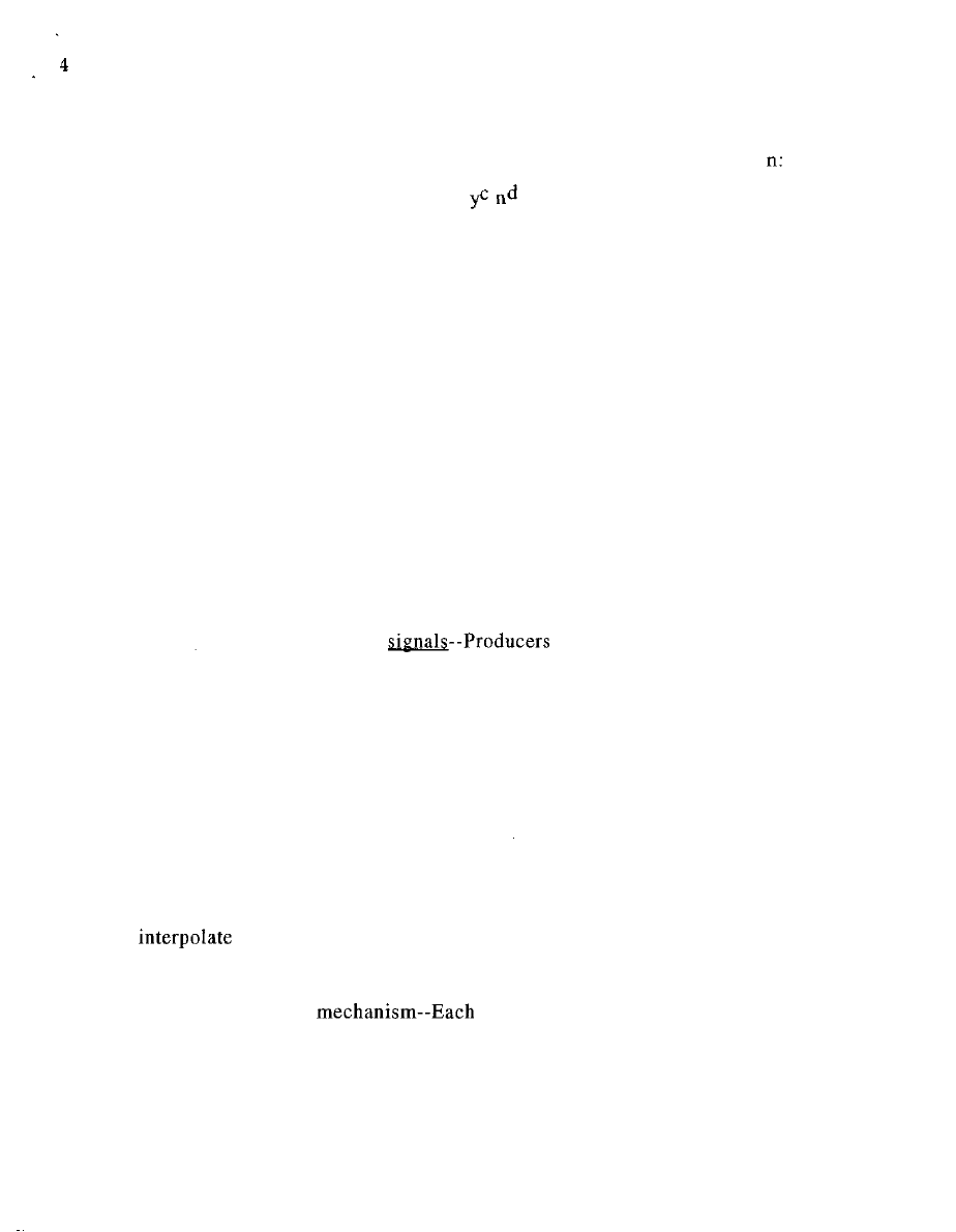
Designate this as C(y; n) for producer with quality niceness level
C(y; n) = q
(1)
Here q is just numerical calibration, and the curve with y is
described by the power c to which y is raised—curving upward when
c > 1, and linear when c = 1, and curving downward for c < 1 (so
marginal cost decreasing). Set n to unity for the lowest quality
producer. To calibrate quality n just from the cost side, set the power
d to unity: the cost structure of each producer then just multiplies
the power of y times the cost scaling q of the low cost producer,
times n.
How do producers decide their commitments to scopes y for
downstream delivery?
Revenue profile as
signal each other, and
buyers, through their set of observed volumes and associated
revenues from the previous period. Figure 2 has no markings for
upstream valuations exactly because the producers are in a fog of
uncertainty as to these valuations. They may not know the cost
structures of their peers and in any case they cannot read these as
direct measures of their qualities as perceived downstream, which
remain mere speculation within the fog of uncertainty. Instead they
through the set of observed (volume, revenue) pairs to
establish a revenue profile, W(y), that frames the choices of each.
The market
producer chooses from along
W(y) that volume for its own n, call it y(n), that maximizes its net
after subtracting its cost curve from the common revenue profile.
However, that set of choices will be validated by purchase
downstream if and only if the downstream is as happy with one
producers choice as another's. That is, there must be some tradeoff in
quality and/or volume between producers' offerings to make them
equally attractive downstream.
Modeling viable market
the y(n)s of a
market's firms are observed to fit along a revenue profile at locations
where its slope indeed matches the slope of that firm's cost curve
(see equation 1) at that y(n). We want to know whether Thai market
remains viable, and with what if any change in revenue profile with
number # of firms, and in their array of cost scalars,
q
This surely may depend on the unknown details of how
downstream valuates these different firms and their offerings.
To investigate, specify a flexible form for valuation as seen by
the downstream. Cast it akin to equation (1), and let Salability
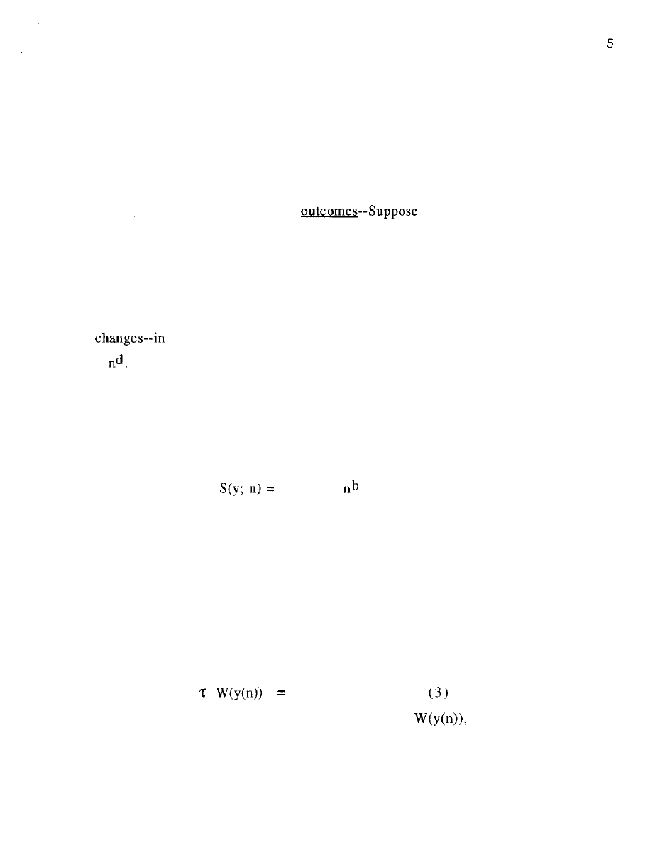
downstream of firm n's production volume y be
(a q) ya
(2)
Here we express the sizing constant as a multiple, alpha, times that
for cost, so that the whole model scales up from the lowest cost level
among producers (q times n=l). Now one could choose b=l if one
wanted quality to calibrate on the buyer side rather than the cost
side: it seems prudent instead to keep both b and d general.
The firms are then offering equally good deals in buyers
collective eyes if and only if
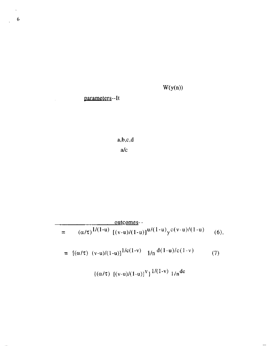
S (y(n); n)
The point is that the offerings, y(n) for revenue
from
various firms each is at the same markdown, tau, from the
corresponding buyer valuation we hypothesized. The crux is that
each firm has found an optimum niche, by its own self-interested
choice, even though the revenue curve W(y) does not refer to quality
distinctions n at all; this is because of the counter-pressure from the
buying side for equally good deals across the combinations of volume
and quality being offered. Hereafter, simplify
to W(n).
Ratios of
is straightforward to verify, by
substitution, that the forms for W(y) and the associated y(n) given in
equations (6) and (7) below will satisfy the conditions given above
for viable market. To penetrate the formalism, it helps to have
grouped the four parameters
into two ratios:
v =
(4)
and u = b/d (5)
Note that a,b,c,d appear in the formulas almost entirely in terms of
these two ratios. This is a basic finding: what the market outcomes
are (and their viabilities) depends on the ratio of downstream to
upstream sensitivity, on volume and on quality.
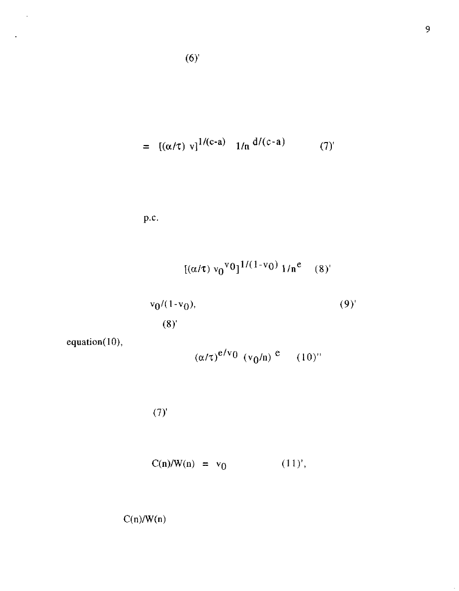
Formulas for market
W(y)
q
along which the choices made by firms of various quality n are
y(n)
as to volume, with the associated revenue to the firm being
W(n) = q
(8)
where here to simplify notation we labeled the power of n as e:
e = (v-u)/(l-v). (9)

And without loss of generality, the magnitude of d can be set to
unity; so we can rewrite equation (8) further as
W(n) = q
(10)
Equation (10) is central in all that follows.
To get a better intuitive understanding we will build up to
these results from a special case, perfect competition
that is
b=0. But already some important features are manifest: Both the
W(y) and the particular W(n) are calibrated by the monetary scale q
from the lowest cost producer. Higher quality producers scale down
in revenue according to the ratio of their quality n to the n=l for
lowest cost, but as raised to a power e in which the volume and
quality sensitivity ratios v and u are
equation (9).
Neither n nor the volume y are expressed in monetary units of
course.
The market sizes, equations 6-8, depend crucially on the ratio
of alpha to tau. Think of this ratio as the scope for building a market:
in terms of Figure 1, the ratio calibrates how far below the upstream
valuations are the downstream costs which must be more than
covered from upstream receipts. The alpha numerator just records
the ratio of downstream to upstream operational scales.
The denominator tau indexes how the market mechanism has
worked out: the deal each firm offers must be equally good, but the
size of this common ratio tau is not constrained. The size of tau is a
path-dependent outcome, which therefore might become a tunable
parameter under influence of strategic manipulations by
participants. The crux is that, contrary to some orthodox claims,

market outcomes are not determinate even when the so-called
side is specified (as for example in equation 2 above).
The technical challenge is to understand dependence of
outcomes also on intricate interpenetration of u and v sensitivity
ratios, which we see as basic descriptors of the contexts, upstream
and down, in which the set of # producer firms of various qualities n
have come to operate as an industry.
So far, each firm's quality contributes through an independent
multiplicative factor to its, and thus to total, market revenue. But this
simple multiplier status for quality will disappear, and the discount
factor tau will become elaborated as a path-dependent fitting factor
rather than a tunable parameter, in the course of generalizations
later beyond perfect-competition characteristics (Section II) and to
include cross-stream substitutability (Section III).
Perfect competition as both prototype and special
producers cannot exclude that the buying side in aggregate sees little
or no difference in quality. They remain in a fog of uncertainty even
when a lecture room theorist might declare them in a perfect
competition market. The downstream side of course encounters them
as distinct firms and also evaluates increments of flow differently at
different overall levels y: this proves sufficient to trigger the market
mechanism. Yet since there is no explicit quality differentiation, the
parameter b, and hence the ratio u must be zero.
The solutions in equations (6-10) still hold, the forms
simplifying to:
W(y) = q
The formula for W(y) in
appears much simpler than in (6), but
industry observers would not see any reason in the field to
distinguish one from the other; nor would they see that only a, not c,
affected W(y).
Next use u=0 to reduce equation (7):
y(n)
The y(n) in equation (7) are seen to depend on both a and c, despite
W(y) depending only on a.
Thence from equation (8) come the observable revenue sizes
sustained in the
market for the firms with the different cost
structures of equation (1). Since u=0, v is designated as VQ in the
simplified form of equation (8):
W(n) = q
The parallel simplifications
e =
and thus e/(e+l) = VQ
ensure that equation
already is the simplified form of
which can be rephrased also as, still with u=0:
W(n) = q
Pause to examine what the costs paid out are by each firm:
substitute equation
into the definition of C(y; n), equation (1).
Routine calculation shows that for each n the cost is the same fraction
of that revenue W(n):
which is to say that the profit percentage is the same for all firms.
Indeed this is also true even when u is not zero:
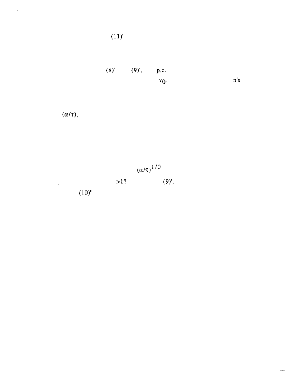
= (v - u ) / ( l - u ) = e/(e+l). (11).
10
One can trace (11) and
mathematically to W(y) going to zero
when y=0. Section II offers solutions where W(y) has a non-zero
intercept and thus firms can differ in profitability.
Using equations
and
the
market outcome can be
specified just from the single parameter
along with the set of
that each enter into a factor, and along with the monetary scaling q,
and the scope scaling (a/T). When VQ goes to zero, regardless of the
size of
W(n) = q (a/T) (12),
whereas when VQ goes to unity, e goes to infinity which means that
only the lowest cost firm produces, at an amount which is
indefinitely large, given that (a/T) > 1, since
W(l) = q
(13).
What about when v
Then, from
e is negative, which
translates in
to higher cost firms having higher revenues, and
moreover to revenues, surprisingly, going down as scope (a/T) goes
up, and also as v itself goes up. This could only transpire through
some sort of feedback in which firms more than compensate for a
context that appears dampening. Great attention must then be given
to stability, which, in the present circumstances, means examining
robustness of the formal results to slight perturbations in each of the
parameters. By the end of Part II we will see that p.c. with v > 1 is
not viable. But stability of results must be examined in particular
when u is allowed to take some non-zero value, and that we can do
here.

11
Downstream markets with quality
now
then to the introduction of u. Each case of p.c. for a value of the ratio
v, 0<v<l, proves to extrapolate into a whole infinite linear array of
quality-competition markets. Visualize the situation in terms of a
state space for markets: Figure 3, for one region labeled ORDINARY.
-- FIGURE 3 ABOUT HERE --
Left out of the state space are the # of firms and their various values
on quality n: the justification is the separation of n into a separate
factor in the equations. Instead the state space is just a plane, with v
for ordinate and u for abscissa.
The chunk of v axis from 0 to 1 are the possible locations, by
sensitivity ratio
of perfect-competition markets. Consider some
one of these VQ. The basic finding from equations (6)
is that
introduction and increase of quality differentiation downstream, b >
0 and hence also u > o, decreases the market revenues W(n) of each
firm. As one moves to the right with u rising, the W(n) will decrease
and fade out after a bit. To keep the size of W(n) up one can however
at the same time raise the level of v above VQ, which is seen from
the equations to tend to increase W(n), thus making up for the
decrease with u.
Geometrically, one expects to find a diagonal rising from the
initial point on the p.c. axis as the locations for similarly sized
markets. That is just what equations (9) and (10) tell us. The slope of
this diagonal, which must be a ray, a straight line passing through
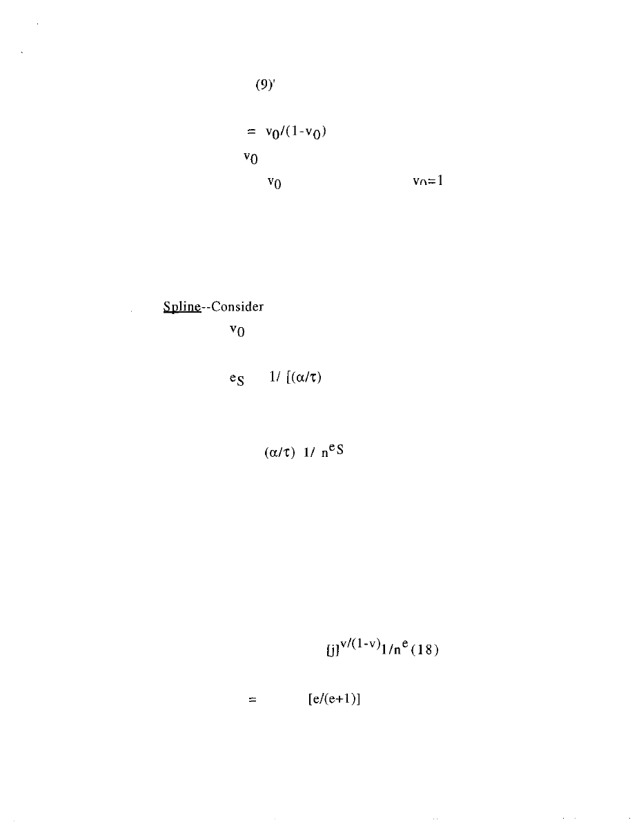
the central point (u=l,v=l), is just the e of equation (9). Note that e is
the power to which n is raised, which thus is a constant along the
12
whole ray. And equation
for p.c. tells us that this common value
is
e
(14)
since the ray begins at
on the v axis, where u=0. Note that the
range of e is from zero, for
= 0, to infinity, for
.
Figure 4 will report the variation of W(n) with v along two
rays, each with e held at a constant value. These examples lie above
and below a special median ray.
The
the special case where
= T / a = e/(e+l) (15)
and so the slope of its ray is
=
-1] (16)
which for example would be unity when alpha is twice tau.
And W(n) reduces in equation (10) to exactly
W(n) = q
(17)
The Spline divides in two the narrowing cone of locations of
viable markets in the u,v state space whose vertex is at (1,1). As u
increases towards 1, the full variation of e remains, but it is so to
speak squeezed into a narrowing cone of context designations. Above
the spline, the sizes of market revenues are larger, whereas they
trail off on the rays below the spline: this becomes obvious from the
following recasting of equation (10):
W(n) = q (a/T)
wherein the auxiliary j is defined by
j
(a/T)
(19)

13
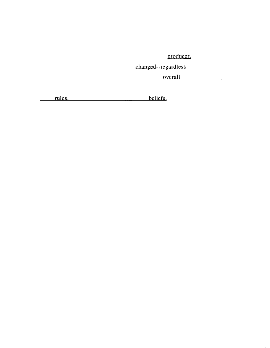
On the Spline j=l, above the Spline j > 1 and so obviously W(n) is
greater, for every v, than the constant value, equation (17), that it
takes along the Spline. And conversely when j < 1.
Remember also that the leverage of higher quality on revenue
goes down as e goes up, as one moves from below to above the
spline. So market shares are more unequal in contexts where the
absolute sizes of producer revenues are going up. And equation (11)
notifies us that profitability goes down,
approaches unity,
also as e goes up, with profitability going to zero in the limit as e
approaches infinity, for v=l.
Figure 4 graphs the size of market revenue W(n) along a ray
for three different values of the extrapolation slope, e. The middle
FIGURE 4 ABOUT HERE -
one is the Spline and so is of course a constant level. Each of these
illustrative rays is continued on through (1,1) to the upper right
quadrant, to which we now turn.
The jump to ADVANCED markets
The most startling prediction from this model is the existence
of an additional whole cone of contexts on the u/v state plane which
sustain viable markets which can generate much larger revenues
than discussed above. Participants themselves of course do not think
in terms of such a state space, which cannot be derived from
evidence they can observe. Rather, producers grope through the fog
of uncertainty in business reality, relying on signals from each other
to frame their commitment choices to volume of production, that are
disciplined by downstream insistence on equally good deals. This
14
counter pressure for equally good deals emanating from downstream
interlocks with the producers' own self-interested choices to
maximize profits: the result is niches for each
volume
choice that cannot be unilaterally
of
speculations about how much production the
context of the
market might support for any given producer. Social mechanism is
what
not final causes or ultimate
in this as in other
configurations from social construction.
A jump is required to reach this additional, upper cone from
the lower one. See Figure 5, which repeats Figure 3 but with focus
shifted to the upper cone in the state space. Mathematically, one can
draw the converging rays on through the (1,1) point, but the
immediate region
-- FIGURE 5 ABOUT HERE --
around this pivot point are contexts without enough playoff between
u and v to sustain market discipline. It is only spread between u and
v, together with their divergence from unity, that through the
signaling mechanism sustains discipline as market niches.
Most of the statements about the lower cone of diagonal rays
through (1,1) are reversed in the upper cone--as indeed the
geometry of rotation around (1,1) as pivot would suggest. The
diagonal ray, from (1,1) through the origin (0,0), in its upper part
still has e=0 and so still has equality of market share across
producers. But now that is also the ray along which the sizes of
market revenues are largest.
Return to equation (10): the crux is that throughout the upper
cone v is greater than unity; so a flip of numerator with denominator
15
is called for in the initial
the factor in quality n is
unchanged.
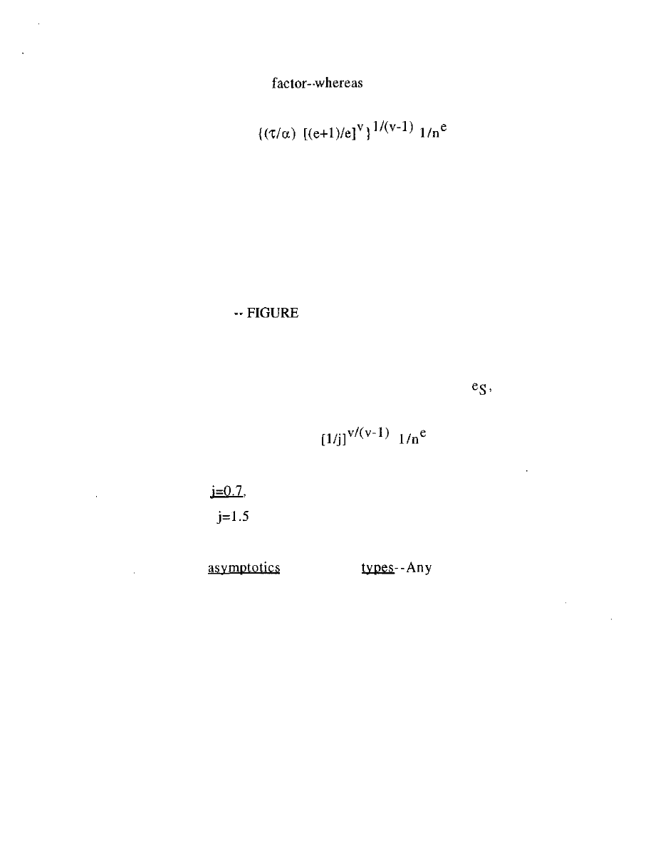
W(n) = q
(20)
One sees at once that as e approaches zero, the main diagonal, the
W(n) predicted increases without limit. The term in tau and alpha
now is less than one, is inverted, being counterbalanced by the ratio
in e being greater than unity.
What remains the same is the Spline; equations 15-17 continue
in force along the whole diagonal. Figure 6 parallels Figure 4.
6 ABOUT HERE --
Note it is still the upper half above the Spline that has larger
revenues for firms, but now from the geometry these are for smaller
rather than larger values of e around the spline value of
equation
(16). Within equation (18), j flips over in parallel:
W(n) = q (a/T)
(21)
Thus note the jump up. across discontinuity at v=l=u. in revenue
along the ray for
and conversely the discontinuous fall in
revenue along the
ray.
Borderline
and ideal
mathematical
model idealizes empirical messiness to some extent. Certainly the
stereotype shapes of equations (2) are hypothetical ideal types for
capturing the central features in variation of valuation with volume
and quality. This is less true of equation (1) since in practice the
producer's decision tends to depend on rule of thumb rather than
elaborate formula. The precision achieved through these idealizations
is what enables us to trace long and intricate chains of effects leading
to such unexpected predictions as ADVANCED markets.

16
In each concrete market situation the ranges invoked or
perceived by participants, in volume and revenue alike, tend to be
narrow and thus will not strain idealizations. Borderlines in these
models should however be handled with care. Revenues going
infinite along the ray with v = 1 is of course a mathematical
exaggeration, as is precise equality to tau of ratios in (3). A calculus
of asymptotic approximations is necessary to disentangle the
meaning of borderline results such as in equation (13), and for other
boundary lines and points.
Asymptotic analysis around (1,1). confirms that the upper cone,
contexts for ADVANCED markets, indeed must be a jump across
borderline anomalies, a jump up from the lower cone, labeled
ORDINARY in Figure 3. And the v=l ray beyond (1,1) now has market
revenues predicted to explode as v decreases from above 1 to unity,
tending to vanish below unity, just the flip of the situation for the
lower cone.
Missing
back to Figures 3 and 5. How is it that
no viable market solutions have been found for contexts identified
by points in the two other quadrants—upper left (high v and low u)
and lower right (low v and high
The next section will in fact
locate upstream-oriented markets there, but nonetheless why not
also downstream?
Equations 8-10 were introduced with the claim that they
satisfied the upstream constraints of equally good deals while also
giving each producer its maximum net revenue. When, however, we
compute them for points in upper left and lower right this is no

17
longer true. In Section II we propose a more general set of solutions,
of which 8-10 are but special cases. Some of this larger set of
downstream solutions will in fact yield some viable markets in parts
of the upper left and lower right, but the maze of complications and
restrictions is best put off until Section II.
MARKETS FACING UPSTREAM
Mathematical derivations for market outcomes come quickly
and easily because they are a particular dual to those for
downstream, and so we can duplicate the ordering in topics and
sections above for downstream orientation. The phenomenology is
also inverted and skewed, however, and that is harder to come to
grips with. The overriding finding will be that upstream orientation
must be evoked to yield viable markets in exactly the other two
quadrants around the center point (1,1).
When producers are jointly confronting and signaling each
other about their upstream, procurement side, the shoe is of course
on the other foot. Instead of seeking revenue from the other side
they are instead making payments. On that side, degree of quality is
supplanted by degree of distaste from the other side, which has to be
paid to provide supplies needed for production volume y! So
producers are jockeying for a niche along the profile of inducement
payments they have to make upstream to support their chosen
volume.
On the other, downstream side, the producers have each come
to think their marketing intelligence is sufficient to predict how
much revenue they will obtain seeing various levels of output, y.

18
Thus each will seek to choose the volume that will maximize the
difference between its known anticipated revenue from downstream,
over the amount they most pay out to the supplier side, read from
their joint signaling profile.
Inverting the
mathematics for downstream
can be turned inside out to yield upstream solutions. For convenience
keep the designation W(y) for the signaling profile, but think of it as
wages, since in substantive terms it compares to the C(y;n) that it
would have paid out if upstream was the determinate side. Also
retain the notation of n for quality which still is a two-sided ordering
with different leverages on the upstream and the downstream sides.
The mathematical switch calls for keeping the C(y;n) notation
for the determinate valuation schedule even though that now in
substantive terms is the analog of the S(y;n) schedules above. The
latter, equation (2), are now to be interpreted as negative, avoidance
valuations on the part of the upstream for supplying work hours to
one and another producer, whose working demands correlate with
the quality of their product perceived downstream.
The solution equations are the same! True, the others' side now
are interested in pushing up the signaling curve W(y) whereas the
producers wish to push it down. But still the other side is insisting
that each of the producers offer equally good deals (albeit now in
money received for work sent), and still also each producer seeks to
choose that y for its n that optimizes the margin of its revenue over
its cost.

19
Plus turns into minus. Each producer is choosing y(n) to
maximize the difference C(y;n) - W(y). So profit is now the negative
of what it was in downstream orientation, C-W rather than W-C. Thus
maximization of floating curve, W(y), over determinate curve, C(y;n),
is reversed into minimization.
The market solutions will be strikingly different despite the
formal similarity of the equations. The set of parameters must flip
roles so that d/b, which is to say
corresponds in substantive
terms to the u for the downstream orientation. And similarly c/a,
which is to say
corresponds in substantive terms to the v for
downstream orientation:
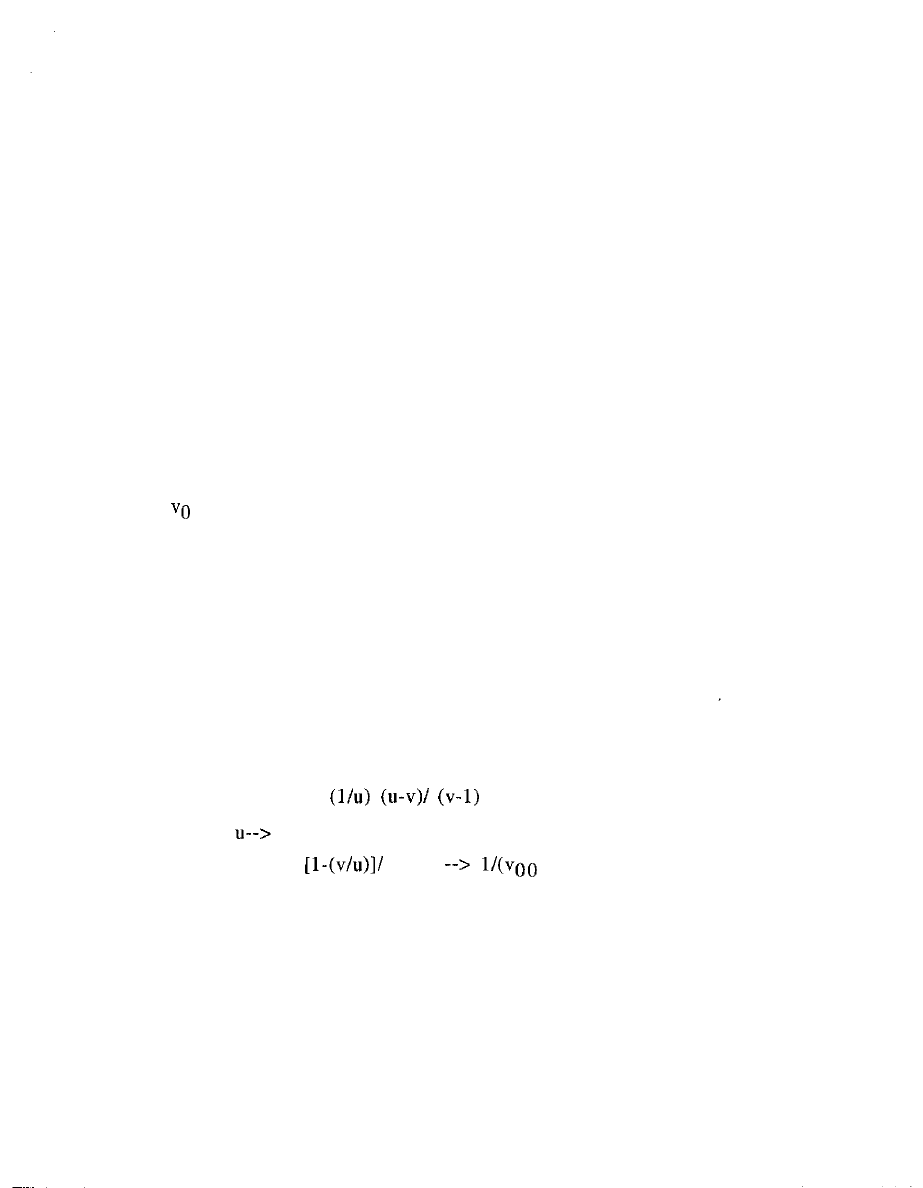
1/u for u, and 1/v for v
(22)
The solution equations 8-10 still apply, but only after the
substitutions in (22), which enable us to position markets in the
same state space, Figure 3.
So, despite some formal parallelism, there are major changes in
viable market predictions, corresponding to real substantive
differences between market mechanism upstream and that for
downstream orientation. Once again, and indeed especially for
upstream orientation, intuition can be guided by starting from the
array of special cases in perfect competition.
Perfect
in dual
is both prototype and special
case for upstream-oriented markets—Each of the producers is now of
course differently perceived on the downstream side, as evidenced
by the distinct valuation structures they can count on (still, for
mathematical convenience described by the C function of equation 1).
20
But there can still be perfect-competition in the dual form: namely in
cases when all of the producers are perceived, from the upstream
side in aggregate, as equally unattractive as employers so that
b = 0
(23)
(Equation (23) also applies above for orthodox perfect competition
where earlier b was also set to zero, but the substantive meaning of
b back then was volume sensitivity of downstream buyers). Thus
this dual perfect-competition corresponds to u here approaching
infinity.
Let the subscript "00" stands for infinity; so we examine the
array of p.c. markets with values for VQQ between 0 and 1, just as
for
with downstream orientation, but now out at infinite u rather
than at zero u. Again we will trace out from each VQQ a ray in state
space along which market size will tend to stay the same, now
because increase in v counteracts the decrease in size associated with
decrease in u below infinity.
Again we hope to characterize this ray, rising from a VQQ by
the e defined in equation (8), but only after it is transformed by (22),
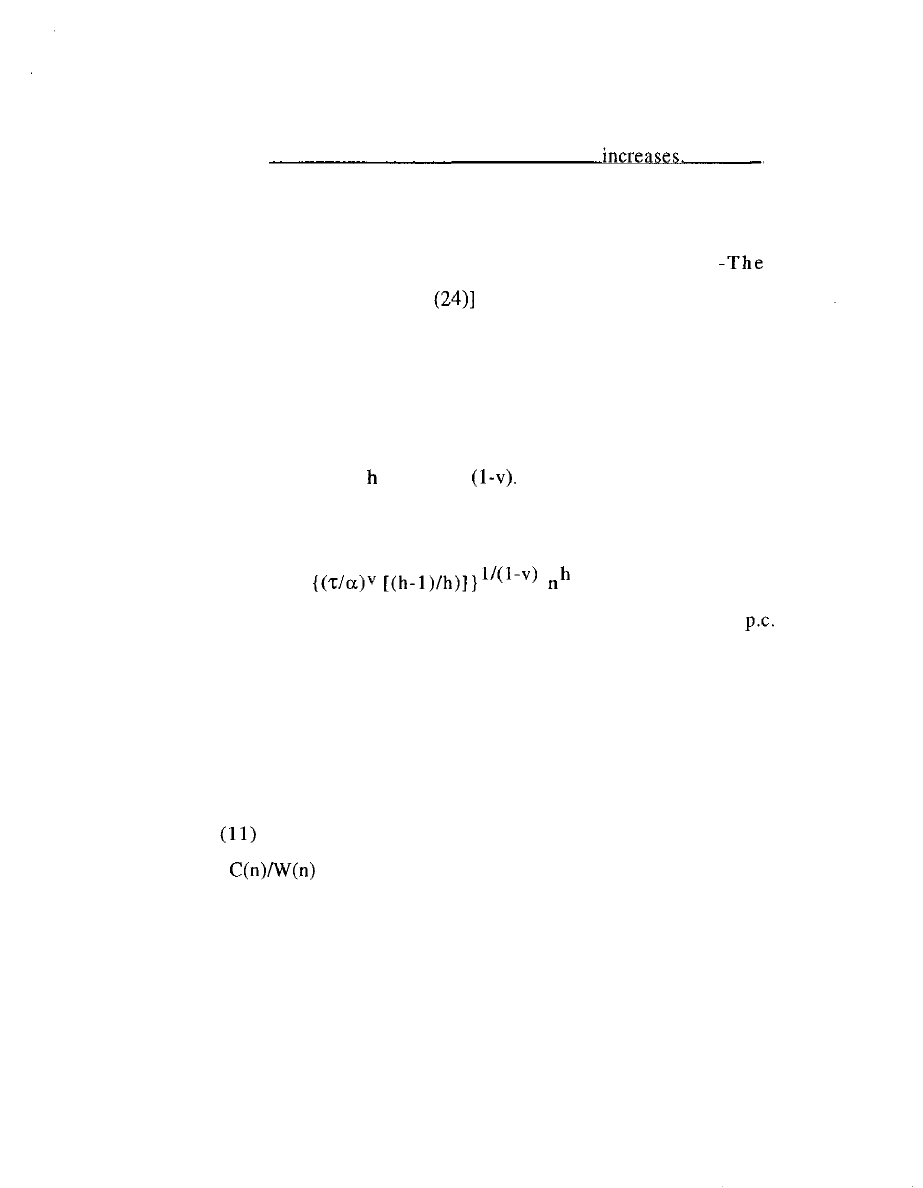
which yields
e =
(23)
and so, as
infinity,
e =
(v-1)
- 1) (24)
Equation (24) replaces equation (14) in calibrating e with the value
of v in perfect-competition, and the solutions for specific values of v
discussed in equations 12-13 for downstream must be adjusted
accordingly.
21
Turn now to variation with parameter u: it will prove to be the
case now that to maintain revenues constant as u
v must.
as offset, be decreased. .
Upstream-oriented markets with quality differentiation-
transformed e [in either (23) or
is no longer a positive number.
It stands for negative slope in the lower right quadrant in Figure 3,
where both u>v and v<l, and on along through (1,1) to upper left
quadrant. To simplify discussion, label the magnitude of this slope by
h:
- e = = (u-v)/u
(25)
The chief equation (10) becomes, for upstream orientation,
W(n) = q
(26)
This is referred to the lower right quadrant which abuts the dual
Its form mixes features from downstream orientation for both
equation (20), which refers to the upper right quadrant, and
equation (10)
Remember, the W(n) is now the cost, say the wage bill, rather
than the revenue of the firm as it was in equation (10). And indeed
equation
translates into
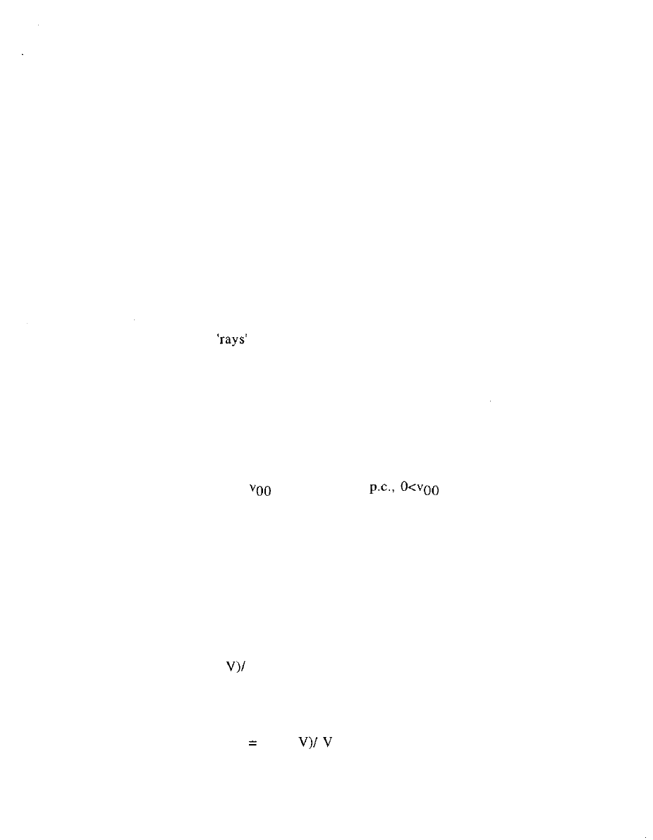
= (u - v)/u (u -1) = h/(h-l) , (27)
still a ratio fixed along a ray, but now with C larger than W. Note that
the q used as baseline scope now in substantive terms calibrates the
high valuations downstream. The scope parameter alpha is now less
than one, a fraction rather than a multiple, given that alpha remains
defined in equation (2) as the ratio to q of the sizing constant for the
22
S(y;n) valuations, which are now reinterpreted as disdain schedules
of the upstream side.
The first striking change from downstream orientation is that
the power to which n is raised in equation (26) is positive, whereas it
was negative in equation (10). This means that higher quality firms
have greater size, in contrast with downstream. Higher quality firms
would welcome a shift of market from downstream to upstream
orientation to increase their market shares.
Parabolic rays and Spline--From equation (25) it follows that
the analog of the
for downstream are now parabolas, although
they too run through the central point (1,1). Visualize the situation as
in Figure 7, with h as index for the parabolas. Figure 7 repeats the
(u,v) state space of Figures 3 and 5, but enters results on markets
oriented upstream.
- FIGURE 7 ABOUT HERE --
Each value of the ratio
, for a case of
<1, proves to
extrapolate into a whole long curve that arrays quality-competition
markets of similar size.
Each parabola is calibrated by an equation to its value of h. The
formula is simplest when u and v are measured from the center:
U = u - 1; V = v- 1;
(28)
w h e n c e
(U -
U (V + 1) = h
(29)
As stated earlier e is the slope of the ray for downstream markets,
which in parallel notation is
e
(U -
(30)

23
which has no product terms in U and V and so is a straight line.
For upstream too there is a Spline. And one could report as in
Figure 4 the variation of W(n) as v increases along a parabolic ray.
Again W(n) is higher than for the Spline in the cone of rays lying
above the Spline, and lower in the lower cone: this is as true in the
upper left quadrant too, for v above unity, where note the ray lying
of course is designated by a higher value of h (analogously to
the discussion for downstream orientation).
This upper left quadrant is designated by TRUSTS in the state
space of Figure 5. Here the buyers downstream are interested in
getting large volumes delivered from their particular suppliers, yet
they do not concede much more unit value to a
from a higher
quality producer. A sugar trust, at least in the old days, or an active
industry producing rather standard metal-work products might fit
there. Turn to a sketch of how these context variations fit together
across quadrants for downstream and for upstream.
and contrasts between upstream and downstream
help intuition to contrast the different configurations of
contexts, that is of sets of valuation schedules upstream and
downstream, which underlie viable W(y) profiles of market signals,
on the one hand for mechanism oriented upstream and on the other
hand for that oriented downstream. Figure 8 provides visualization.
A small duplicate of the state space common to both orientations
appears in the center of the figure. An arrow leads from each of
these quadrants around (1,1) to a stylized set of upper and lower
valuation schedules (downstream valuation and upstream cost).

24
- FIGURE 8 ABOUT HERE --
Just four producers are shown, rather evenly spaced on quality.
Rather extreme values of a and c compatible with a given ratio v are
used so as to heighten contrast. The key is the trade-off of that
contrast with, on the other hand, the contrast in growth of the
vertical (monetary) placements of the a curves and the c curves—
which is set of course by the relative sizes of b and d. (Since
designations of curves by C and by S are switched between reporting
upstream and reporting downstream orientation, they are omitted.)
Overlaps and contrasts between upstream and downstream
approaching and on the ray v=l are contexts
where both downstream and upstream solutions are predicted. The
contrast between solutions is striking, and this contrast switches
according to whether u is greater or less than unity. With upstream
orientation markets are predicted, when
to yield very large
W(n). Whereas along this same half of the v=l line, downstream
markets are predicted small. Just the reverse obtains for the part of
ray for small u, less than unity.
The u=l ray, the vertical through (1,1) in Figure 7, is, on the
other hand, the province solely of upstream oriented markets, since
in the neighboring region where their sway does not hold neither are
there any downstream markets. Above v=l, the sizes W(n) tend to be
very large. For v<l on the other hand the W(n) tend to be small. Both
these are results from the previous analysis around upstream Spline

25
and other hyperbolas (with the u=l line, when adjoined to the part of
the v=0 line beyond u=l, being seen as a degenerate extreme of the
parabolas).
Extreme values of ratios come from extreme values of
individual parameters, with c=0 yielding v=infinity, and a=0 yielding
v=0. Zero value of an exponent corresponds to zero variation, that is
to constant cost curve C(y;n) and valuation curve S(y;n), respectively.
In general, the market signaling mechanism should be applicable
even when one or the other of these constituent valuation schedules
is constant. This corresponds, in Figures 1 and 2, to horizontal lines
for the C or the S. Examine equations (10) and (26) for the
downstream and upstream solution rays. For v=0 the W(n) shrink to
zero, disappear in both equations and thus for all of the state space
with u positive. However, in the PARADOX region, u negative,
equations (10) and (26) are transformed by the flip in sign of u so
that W(n) takes the value (q/n). with upstream orientation and the
value (q
n ) with downstream orientation. The divergences
within sets of constituent valuations (see Figure 8) are great enough
to sustain the mechanism even with one of the sorts being a constant.
Comparison with other socioeconomic
in
these network flows can continue amidst chaotic scramblings by
entrepreneurs exploiting networks of social relations, as theorized by
Burt (1993). In contexts in the center of the state space, Figure 3,
analysis surely is called for, and Fligstein's interventions by
the state also may be expected there. Podolny (2001) develops a
phenomenology of uncertainty in relations across a market interface.

26
His classical two-by-two table of market types seems to correspond
to the four regions in Figure 3 demarcated by the main diagonal u=v,
and the ray v=l. See Figure 9.
- FIGURE 9 ABOUT HERE -
The four can, when framed by a state space, be seen as complements
(a fuller account can be found in my paper included in Breiger
Other socioeconomic approaches, in particular the population
ecology line of Hannan and collaborators, are harder to compare
because they focus on perceived attributes of individual firms rather
than identifying market role clusters as the key to context. The
niches they speak of, recently in Dobrev, Kim and Hannan (2001), are
like niches in pick-up games in parks rather than competitive niches
within an architecture of teams (cf. Leifer 1995). The W(y) model can
be seen as invoking "middle-status conformity" (Phillips and
Zuckerman 2001) on the level of firms rather than managers.
PARADOX: THE OTHER HALF OF CONTEXTS, FOR MARKETS
FACING EITHER UPSTREAM OR DOWN
The state space shown already in Figures 3. 5 and 7, should be
doubled. The W(y) signaling profile can work to broker between
upstream and downstream whenever the producers are arrayed in
the same ordering (not actual spacings) from both upstream and
downstream perspectives. For a market facing downstream this
raises the paradoxical possibility that as quality of goods produced
goes up the cost structure is going down. This means that the ratio u

27
can be negative (either the b or the d can be calibrated as negative).
Figure 10 reproduces Figure 5 and extends it to this negative half
plane.
-- FIGURE 10 ABOUT HERE --
Once again, as in the switch to upstream orientation, the
mathematical solution is easy: just introduce the minus sign into the
equations already given above. And yet once again the substantive
outcomes are surprisingly different. Intuition as to that can be
guided by inspection of the strikingly different contexts, sets of
valuation schedules, being invoked: see Figure 11, which is parallel to
Figure 8.
-- FIGURE
ABOUT HERE --
There are three striking differences. First, so long as u is
negative, call it the PARADOX region, the signaling mechanism does
not work to yield viable market solutions for any v > 1 (as
throughout this Section I the details of failure are postponed until
Section II). Second, the dependence of market revenue for a
producer, W(n), varies in inverse fashion with n to what obtained
with u being positive. The third difference is perhaps the most
instructive: at every point with v<l and u negative, the signaling
mechanism works both with upstream orientation and with
downstream orientation.
And yet there is also remarkable commonalty with results for
the u>0 half: PARADOX markets also all are extrapolations of
indeed extrapolations of both the dual forms. Figure 10 shows this
graphically by extending both the downstream rays and the

28
upstream
former from the u=0 edge and the latter
from the u=00 edge, into and through the whole length of PARADOX.
What this means is that the very equations for y(n) and for
W(n) already given above apply for u<0 also. It is the reversal of sign
of u that leads to the second major difference just cited. (One could
argue that PARADOX is no longer an apt label for these contexts
when market orientation is upstream, since then the W(n) of higher
quality producers is indeed lower, through the upstream view of it
being more dismissive.)
substance and modeling
Producers cope with uncertainty by orienting to the
commitment choices being made by their peers that get supported
by another side. The other side's acceptances rest both on its
sensitivity to volume and on its sensitivity to differential quality
across the producers. Equation (10) is the key throughout, reporting
the revenues that producers select from along their joint offer curve,
each in its own self-interest.
This jointly perceived offer curve, W(y), may be turned and
twisted in various ways, which we observers relate to context. We
summarize context by a few parameters arrayed into a state space,
taken together with the set of qualities. All the various regions of
state space, and the two orientations, work with this same
mechanism.
How should we understand and interpret quality
differentiation? First, root it in perfect competition, and second, do so
for both the upstream and downstream orientations of market

29
mechanism. The dual upstream orientation satisfies the same
equation (10), once one switches labels of W with C, along with
inverting the sensitivity ratios. Along any ray through (1,1) in state
space, the leverage of quality on revenue remains fixed across the
whole range of v.
The jump to a volume sensitivity ratio v greater than unity
flips the signs of exponents, so that the multiplier of quality switches
dependence on context variation, which can open up dramatically
larger outputs, the ADVANCED region. The other PARADOX half of
state space accommodates both upstream and downstream
orientation, in each case just by reversing the sign of quality
sensitivity ratio u from plus to minus.
Aspects of
to the initial Figures 1 and 2 that
motivate the whole model. A key role is played by the relative
sensitivities of valuations to volume between upstream and
downstream contexts of the producers. Thus, ratios rather than
actual exponents are what count, so that for instance constant
returns to scale, c=l, does not need separate treatment, nor does a=l.
Observe that the mathematics can be kept elementary, just
undergraduate calculus plus persistence. Use of special forms for
valuation schedules permits tracing complex chains of causation, such
as we traced to ADVANCED operation of markets. And yet, by
principles of analytic continuity, even as topology changes with
schedule forms one can expect the main features of solutions to be
generalizable. Intricate patterns of fitting are the key, not formal
generality.

30
We now go on to two major generalizations which, however,
will still keep equation (10) central.
//. MARKET OUTCOMES WITH PATH DEPENDENCY
Take observations of some particular market of say #
producers that runs on the signaling mechanism, that meets the
constraints laid out in Section I. From observing just the volume and
the revenue of each producer, together with the slope observed there
(either that of its cost curve or of the W(y) there), from just these
three numbers, for each of the producers of number #, one can
derive estimations for all the
n for each producer,
together with q and a,b,c,d and thence u and v and e. Without loss of
generality one takes the lowest quality as n=l and for convenience
set
The one slippery point, on which we expand in Section III,
is fixing tau and alpha. In fact only their ratio, a/T, can be estimated
from the observations of the one market.
The main point is that the outcomes for this observed market
will not in general fit the predictions from the equations in Section I.
The extrapolations from perfect competitions limited the possibilities
unnecessarily. In reality the process by which a signaling mechanism
settles in for a given context is a path-dependent matter of
adjustments and readjustments.
Return to equation (6), which is indeed sufficient but is not
necessary for a viable solution. See White (2002, chapter 2) for a
For details see the first seventeen equations in chapter 8 of White (2002).
31
derivation in elementary mathematics of the necessary and sufficient
form of W(y):
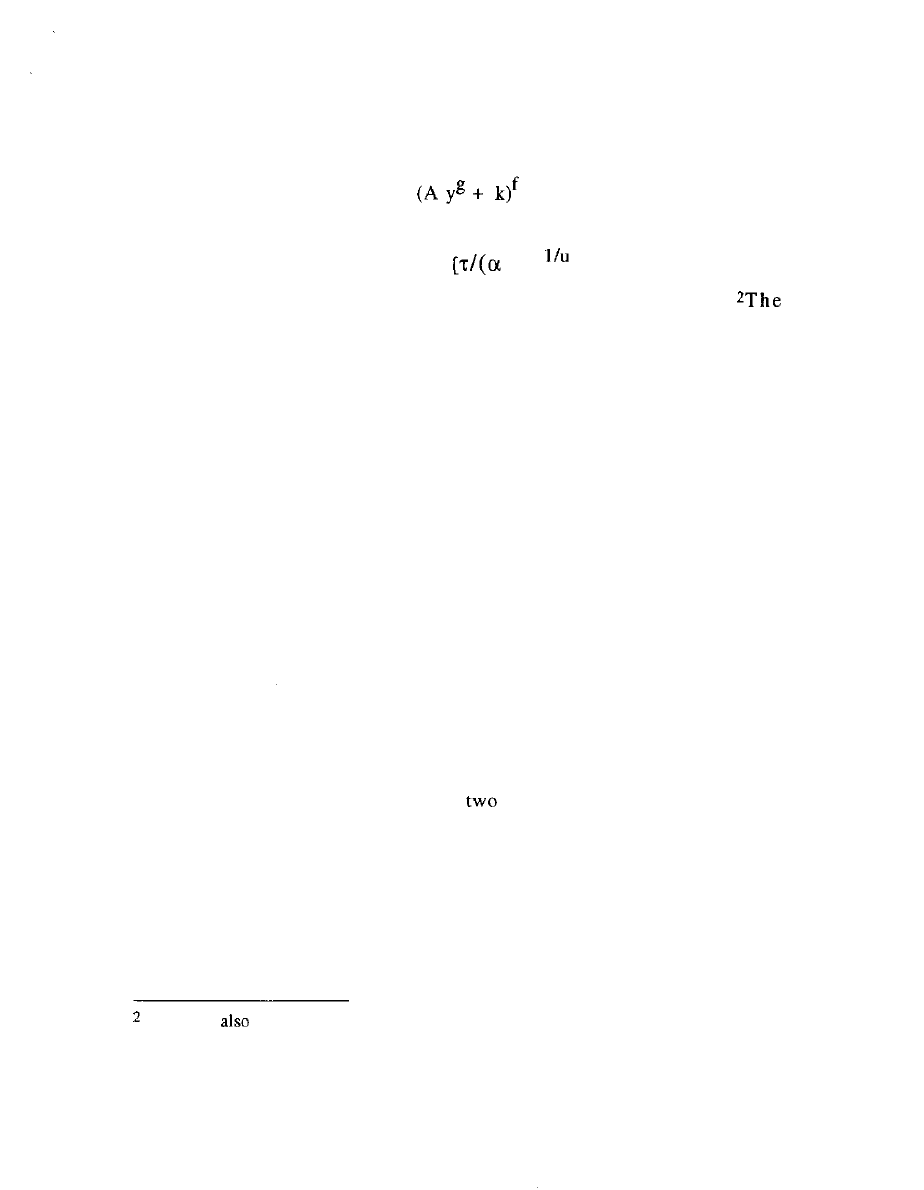
W(y) =
(31)
with translations into the previous parameters as follows
f= u/(u-l); g= c(u-v)/u; A= c
q)]
(u-l)/(u-v) (32)
so that only k, as numerical index of the generalization, is novel.
substantive point corresponding to the mathematical fact that the
solution contains a constant of integration, here named k, is that
there may be a whole plethora of satisfactory solutions in addition to
that in equation (6), which is seen now to correspond to k=0 in
equation (31).
Return to the observations on a concrete market. One can at
once estimate k, from the observations on any one producer plus the
parameters above aside from the set of n's. But the model should be
able to tell us which values of k will work. We have already seen
with Figures 3, 5, and 7 that there are whole ranges of contexts, that
is point in state space, for which k=0 does not yield viable solutions
and any other particular value of k, being less central and not a
continuation of p.c., is presumably more exposed to rejection.
Let us develop systematically
further tests for viability of
market mechanism beyond those enforced explicitly in Part I: first,
for whether W(n) yields an extremum for that producer, and second
whether the extremum indeed yields it positive profit. For both
orientations the solution equations in Section I already guaranteed
the slopes of W(y) and C(y;n) to be equal at y(n).
One can
consult Spence (1975), where this result is obtained from partial
differential calculus, and White (2002), where elementary calculus is used.

32
For downstream orientation, with W(y) being revenue, the
must be a maximum, so that the first test if that the
second derivative of W-C is negative at y(n). Whereas for upstream
orientation the first test becomes that the second derivative with y
of W-C be positive, so that the distance of its negative, of C above W,
is maximized. For downstream orientation positive profit means W>C,
and the reverse for upstream orientation.
Calculations show that the first and second tests can each be
expressed in terms of inequalities which k must satisfy. Each
inequality takes a different form in the distinct polygonal regions of
the state
Figure 12 reports the range of k values allowed by
region, for downstream orientation, and Figure 13 does so for
upstream orientation: note that each, like Figure 10, includes the
whole PARADOX half.
-- FIGURE 12 ABOUT HERE -
- FIGURE
ABOUT HERE --
Note that k=0 is indeed allowed in and only in those regions
where solutions extrapolating
have been reported earlier. In
particular, PARADOX is the only region wherein k=0 is allowed in
both Figures 12 and 13. Our main business is to explore the solutions
where k is not zero. For participants in business, surely, the main
issue is how large will the market revenues be. But first, examine
further the bottom right quadrant of Figure 3 state space, for u>l
combined with v<l.
See Table 3.2 in White (2002, pp.54-5)

33
Unraveling by location on
signaling mechanism
has an additional vulnerability. Some producers may opt to offer just
the same output volume, with all other constraints satisfied. This
happens when the W(y) curve with a given value of k does not offer
unique optimizing choice on y to each lower quality producer, who
nonetheless estimate that they will make a profit at the lowest
volume being offered by other producers. The buying side will not
however sustain this and thus turn away from the producer whose
quality does justify that edge volume. So step by step the market
profile of signals is unraveled.
Earlier (White 2002, chapter 4) I illustrated how unravelings
fit with maneuvers by entrepreneurs within these social network
constructions (and see Burt 1993). For upstream orientation this is
especially commonplace for market contexts in the cone marked
ORDINARY for downstream orientation, Figure 12. For downstream
orientation it is especially common in the lower right quadrant that
in the upstream orientation merges into the dual perfect-
competition. Interesting examples can be found, as for road haulage
(Biencourt 2000) and I have labeled this region UNRAVELING in both
Figures 12 and 13.
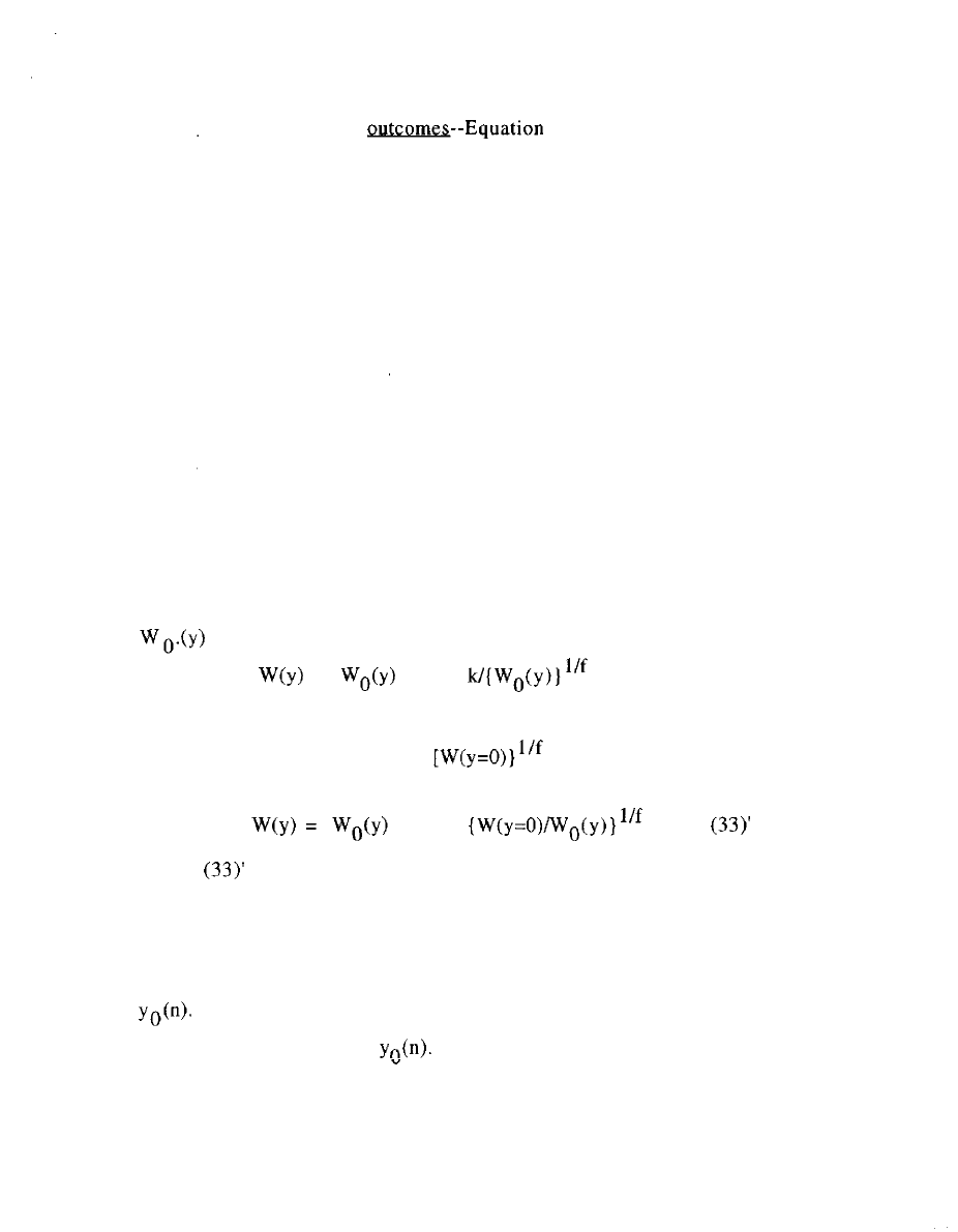
Markets for contexts in any region where unraveling is
common cannot sustain themselves for just any distribution of
quality across their producers. They are especially vulnerable to and
likely to manifest manipulations and maneuverings as entrepreneurs
seek advantage through turmoil that eventuates in
34
Shifts in market
(10) requires numerical
solutions, which can be obtained through a computer algorithm for
self-consistent search (cf. Leifer 1985; Bothner and White 2001). But
the array of possible contexts is staggeringly large so that even
carefully selected sets of examples (e.g. White 2002, Appendix
Tables, pp,. 334-338) give inadequate guidance. Yet, for each context
where the solution for k=0 is allowed for that orientation of market,
insights can be derived.
Asymptotic approximations around k=0--What variations in
revenues result from interaction between k, indexing the path of
evolution, and parameters defining the context? Answers come from
expressing W(n) as a deviation growing as k grows from zero.
The first step is easy and obvious. Designate W(y) for k=0 by
When k is small, the formula in (31) can be approximated as
=
[ 1 +
] (33)
The value of k itself can be expressed in terms of the intercept of
W(y), its size when y=0: k =
So (32) can be rephrased
as
[ 1 +
]
where
like (33) is a better approximation the smaller k is.
Our interest is in the actual market revenues, the W(n), each
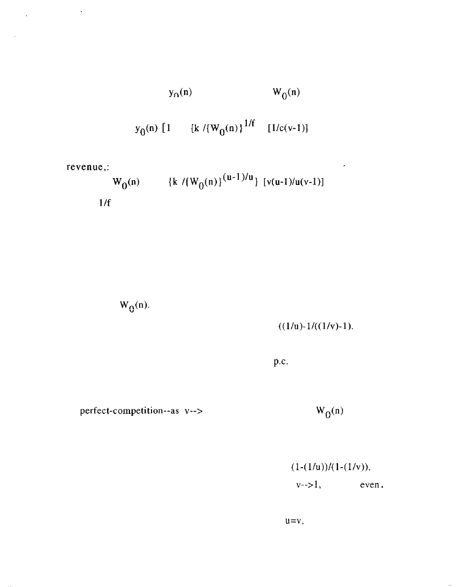
the revenue for the volume y chosen by that firm of quality n, y(n).
Equation (7) already gives us the y(n) for k=0, designate it now by
But a given quality n will yield for any non-zero k a y(n)
which is not the same as
Thus equation (32) is deceptive:
35
We must return to equation (7) and, using (31) and (32)
together with (33), develop first an asymptotic approximation for
y(n) itself in terms of
and its revenue
together with the
k. The result is
y(n) =
+
]
] (34)
Using this we can finally obtain a usable approximation for market
W(n) =
[1 +
] (35)
where
has been written out in terms of u. These approximations
need to be spelled out separately by regions in the state space to
guide understanding of the effects of the allowed k shown in Figures
12 and 13.
For example, in the ORDINARY region for downstream
orientation, we see that, since k must be positive, W(n) is always
larger than
The fraction by which it is larger, for a given
small k, is proportional to the positive ratio
This
latter ratio is, since l>v>u, always greater than unity: it becomes very
large either when u is small, that is along the
axis, or when on
the other hand v approaches unity. So the most important distortions
introduced by non-zero k, are to increase revenues for contexts close
to
1 already the revenue
is
exploding.
Somewhat similar results obtain in the ADVANCED region,
where the ratio just discussed is rephrased as
since now l<v<u. The size of the ratio explodes as
so that
small k leverages big increases in W(n) along the bottom of
ADVANCED region; whereas along the diagonal,
the ratio is just
36
unity so that Section I results are not much affected. The major
difference for ADVANCED, however, is that now negative values of k
also yield sustainable market solutions and these will be reduced
from the corresponding
Turn now to upstream orientation, where the substitutions in
(22) convert equation (35) into a simpler form:
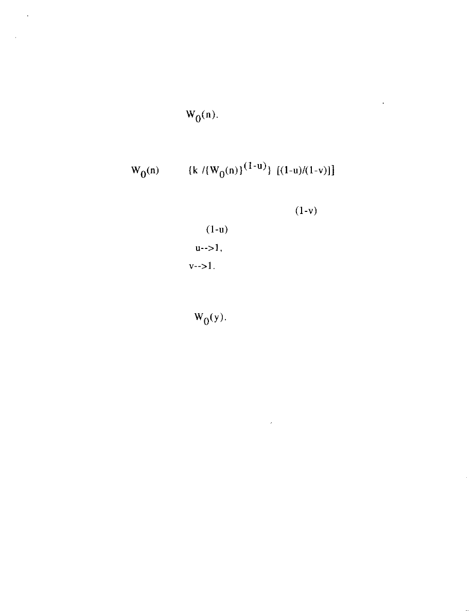
W(n) =
[1 +
(36)
The principal finding is that positive k now always generates
decreases in W(n), since in the TRUSTS region
is negative while
in the UNRAVELING region
is negative. Their ratio will go in
magnitude toward zero as
meaning little impact from k, but
will grow very large as
Remember that in upstream
orientation it is the high quality firms that have the bigger revenues,
that will be boosted most in absolute terms when a signal profile
W(y) is shifted by k from
///. OUTCOMES WITH CROSS-STREAM SUBSTITUTABILITY
What would be effects from substitutability of a given
industry's outputs with those from other markets lying cross-stream,
in locations structurally equivalent to some extent within the
upstream to downstream flows with the location of the given
market? For downstream orientation the most obvious formulation is
erosion of the valuation schedules of downstream buyers (which are
not directly observable, of course).
37
Indeed signs of such
may also appear as
between the separate producers of the given market. Consolidate all
this into one parameter for discount, call it x. Because of such cross-
discounting, the true valuation by buyers in aggregate downstream
must involve interactions between the separate valuation schedules
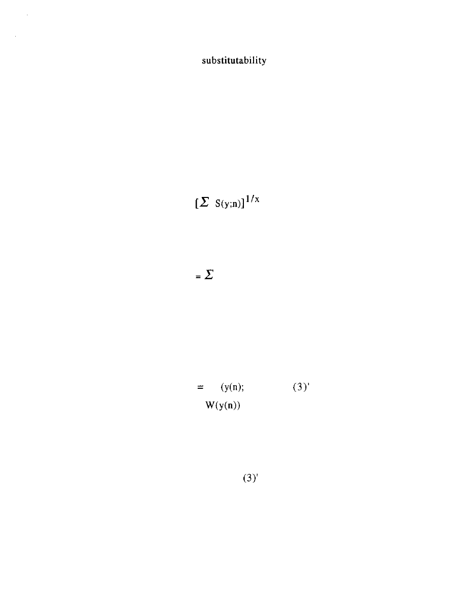
hypothesized earlier in equation (2). Let this aggregate valuation be
designated as V. Approximate it by a discount of a summation across
the separate producer schedules S:
V =
(37)
It is appropriate to then also focus on the overall aggregate
market volume, designate it by W . This is the sum over the
revenues W(n) of all the firms of various qualities n in that market:
W
W(n) (38)
The equally good deals constraint, equation (3), must be retained, but
now its actual numerical size depends on the aggregate market
revenues W . To clarify this, re-label the multiplier in equation (3),
say as theta, now a numerical fitting constant as much as a tunable
parameter: Replace (3) by
0 W(n)
S
n)
where as before we simplify
to W(n).
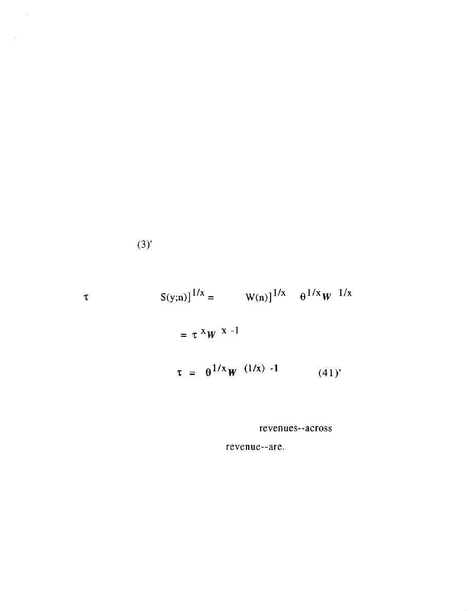
Now transfer use of tau to the aggregate level:
1 W = V (39)
where tau has been put in boldface to signify its being defined for
aggregates. Whereas equation (3) or
emphasizes that each
producer must offer terms equally as good as for the other
producers, one uses equation (39) just to point out that in aggregate
38
the valuation must exceed the revenue paid producers for the
market. That is, equation (39) entails that 1 > 1 .
Some degree of substitutability, x>l, is surely to be expected. So
hereafter we will talk in terms of tau. Tau being unity means that
the profile of revenues W(y) is extracting the most aggregate
revenue that the buyers in aggregate could be pushed into paying for
such menu of deals (not that this maximum is observable).
Yet all the previous equations are expressed in terms of what is
now redefined and re labeled as 0 . We need a translation formula.
Put equations
and (39) together through the use of the
definitions in equation (37) and (38):
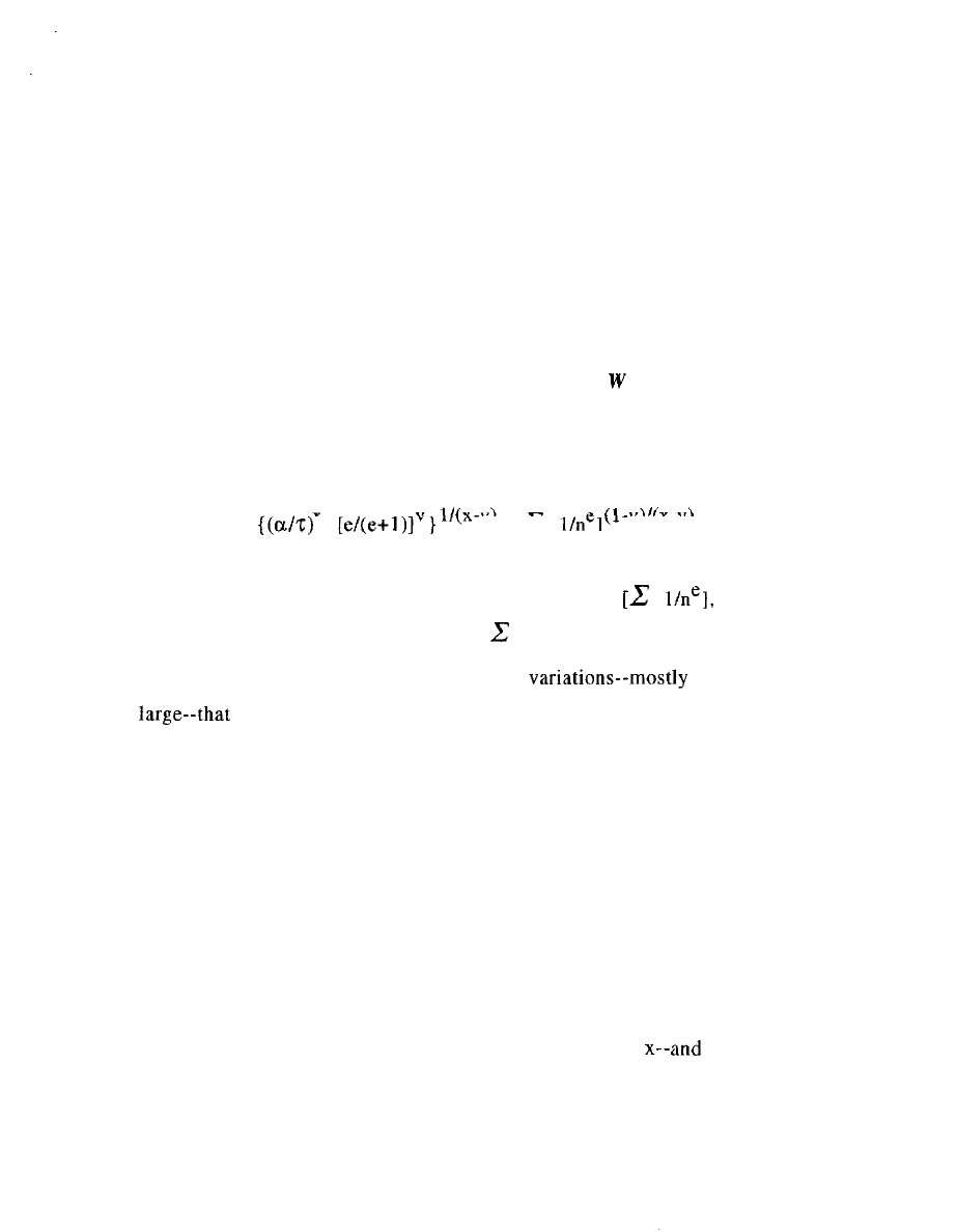
W =V = [Z
[Z 0
=
(40)
so that
0
(41).
the converse being
In substantive terms, equation (41) means that the solutions
for y(n) and W(n) for a producer given so far in fact depend in size
on what the whole set of volumes and
all firms,
and thus the market aggregate
Note that these results so far on substitutability are general
and thus applicable whatever the value of the path constant k is
(Section II). But there is no closed formula giving results for market
aggregate or for individual producers except in the case of k=0, the
39
extrapolation of perfect competition in which all producers have the
same profits and the intercept of the W(y) curve is zero.
We now proceed to derive formulas for this k=0 case as a guide
more generally to the impact of substitutability upon market
outcomes. All we need do is substitute the right side of equation (40)
in place of what we have written as tau in all the equations of the
previous two Sections. For downstream market, substitute equation
(10), with this transposition, into equation (36).
appears now on
both sides of the equation; the necessary consolidation yields, using
the tau defined by equation (38),
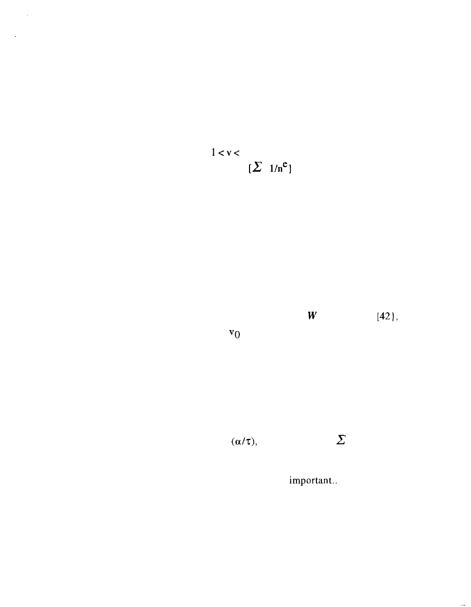
W = q
[
[42}
Quality leverage appears only in a separate factor
which
we can denote for simplicity just by
in Figure 15 later.
Our main concern is to show the
not very
it brings to the results in previous Sections. The Spline
and associated rays, for upstream as well as for downstream, carry
through pretty much, along with the region boundaries discriminated
as in earlier Figures 5, 7, 12, 13 for state spaces, including PARADOX.
Note that the impact of the particular array of qualities, the set
of n's, appears in the aggregate revenue formula also as a multiplier,
the sum raised to a power that combines and thus contrasts the
distance of v below unity with its distance below the substitutability,
x. Indeed the main impact from degree of substitutability is just in
the band in state space where v lies between 1 and
of course
with u >v>l in order to lie within ADVANCED region of viable
40
markets. All the previous constraints on solutions still hold with x
introduced too.
Inspection of (42) indeed shows a curious drop in the
contribution from this quality sum exactly in this band, which we
designate
CROWDED:
x (43) .
In equation (42) the power to which
is raised is negative
in this band. That means, for example, that if new producers (along
with corresponding consumer valuations) are added to the market,
with other parameters unchanged, the market aggregate will
decrease (although within the given aggregate the revenues to higher
quality firms will still be lower). Figure 14 superposes the CROWDED
band onto the earlier Figure 5.
-- FIGURE 14 ABOUT HERE --
Visualize the variation of aggregate revenue
, equation
as v increases from its minimum,
, along a ray through (1,1), for
one value of x, 1.25. Figure 15 graphs W along the central ray, the
Spline. Compare it with the Spline in Figures 4 and 6 earlier. It is in
and near the CROWDED band that substitutability has its impact.
Elsewhere (White 2002b) I have derived partial differential
equations for not only change in W with v, but also for its change
with x and with other parameters,
e, and with the
These
are, however, logarithmic partial differential equations which tend to
conceal discontinuities so that computation is
-- FIGURE 15 ABOUT HERE --
Satisfactory understanding requires also specifying how the
W(n) of individual producers are affected by degree of
41
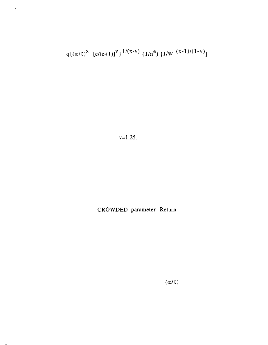
substitutability x. It is straightforward to show that equation (10)
becomes
W(n) =
(44)
One can see that the primary impact from x on any particular W(n) is
an extra multiplier, at the end. This multiplier is the feedback effect
of aggregate revenue and is the same for each of the producers. It is
neutralized when x goes to unity, but will tend to wipe out the W(n)
for v close to unity.
The analysis suggests that W and W(n) ordinarily are not
much affected by substitutability, except for the sharp drop in the
CROWDED band from v=l to
The main conclusion is that
substitutability does not much distort the result of analyses given
earlier assuming x=l. The generalization in Section II to non-zero k is
of more importance, except in the CROWDED band. This is just as well,
for the problems in estimating a value for substitutability x are
formidable.
Identifying the
to the discussion
of estimating parameters for an observed market thought to be
produced by the W(y) signaling mechanism. Already it was shown
impossible, at least with one panel of observations, to identity tau
and alpha separately only as a ratio. The results in this Section III, in
particular equations (41) and (42), now show that even this ratio
cannot be identified separately from the value of x, and conversely.
The estimation equation which packages
with x derives
from equation (40). Section II showed that theta can be separately
estimated from the observed values of y and W and slope for each

42
producer, but only as a ratio to (a q), the scaling factor for buyer
valuations S. And now equations (40). and (41) show that the
observed value of aggregate market revenue W must figure in the
identification of a value for the underlying parameter tau.
The following specifies an equality between an expression in
the ratio of
to its alpha, involving W , and on the other side an
expression in the ratio of tau to its alpha, that involves both W and
x. The point is that it is the same W and q on both sides of the
equation, since the issue is only whether the observed market, with
given aggregate revenue and q long since estimated, are fitted by
theta or instead by tau coupled with some x larger than unity.
/
=
/
/ q] (45)
So the x value required to support changing from no
substitutability is given by (with
for logarithm to the base e)
x
(T
(W
=
+
W (46)
Both terms on the right hand side of equation (46) are observables,
known quantities fitted for that market. If x is chosen to be 1 then of
course the left side becomes identical with the right. But the equation
can only specify a continuum of pairs of value (x, (T
for the two
parameters as sufficient substitutes.
We can now see how to interpret this indeterminacy, in terms
of equation (15) and the basic Figure 4 ( and analogously for
upstream). The central ray, the Spline has its numerical location
on the v axis between 0 and 1 determined by T / a. And similarly for
the numerical value of its slope
. So if one argues that
substitutability is higher than unity, then the location of the Spline
changes, but without disturbing the relative structure of rays in the

43
cone. Earlier we saw in Figures 14 and 15 that, by and large, the
numerical values of W(n) and W were not much affected by
increasing the value of x, with the exception of the CROWDED band
where they were sharply reduced.
The problem has a tendency to correct itself. One is unlikely to
observe and actual market which is in the CROWDED band in state
space because mostly there its size would be so small. Computations
show that when x is increased then VQ is decreased because the
is decreased. But then for v<l the part of the cone above the
Spline with larger revenues is enhanced (and these are not much
impacted by the increased x), whereas for v>l the upper part of the
cone above Spine, again with greater revenues, is
more to the point the lower part with reduced revenues even aside
from the CROWDED impact, becomes a larger share of the cone. So
High values of x are unlikely to be encountered except for markets
with high v.
The CROWDED band which is induced by increased
substitutability x can be lumped with borderlines and regions of
unraveling in the state space where the W(y) market mechanism of
signaling also is not robust. In such contexts the underlying
production work will no doubt get done by some other sort of social
construction. This can range from the intervention of government of
various sorts and levels, discussed by Fligstein (2002), to
organization through tradition along kinship or patrimonial lines: see
earlier discussion around Figure 9.
APPLICATIONS

44
In their recent reviews of Markets from Networks , sociologist
Fligstein (2003) and economist Loasby (2003) both call especially for
empirical applications. Some applications of W(y) models were
reported in the book (White 2002) and earlier: see e.g.,
(1992,
chapter
Leifer (1985) and White (1981). A couple of other
applications have been published since the book went to press:
Biencourt and Urrutiaguer (2002); Bothner and White (2002). The
present paper offers a compact, yet self-contained guide for further
modeling. The increased emphasis here on the dual orientations of
markets should encourage extrapolation to macro-economic topics
(e.g., White 2002d, 2003a) and especially labor markets. The explicit
rooting of quality competition in perfect competition clarifies the
phenomenology, and bears on the admirable dissection by Favereau,
Biencourt and Eymard-Duvernay (2002), who pay particular
attention to labor.
Fligstein suggests that W(y) models suggest how industries pull
themselves apart into distinct new industrial role sets, and Bothner
develops this same idea (Bothner, Stuart and White 2004). Fligstein
calls for applications to particular industries and sectors. In
collaboration with a French team (Chiffoleau, Dreyfus, Laporte, and
Touzard 2003), I am engaged in a multi-year study of their wine
sector. Interim results (White 2002b, 2002c, 2002d) include
technical simplifications to ease use of conventional data on average
market prices, as well as substantive extrapolations.
Long-term tracing of a particular sector and its industries is
promising. King (2003) offers preliminary results for the dairy sector

45
in the U.S. from the 1880s through to World War II. As for the
French wine sector, heavy influences from cooperative organization
forms and from regional specializations complicate the analysis. Still,
one of the new phenomena predicted by W(y) models may be
recognizable. King came to focus on the processed cheese industry,
for which the contexts in this era, when consumers valued more
what industrial operations made with less expense, appear to fit into
PARADOX region. This is the only region of state space (Figures 5, 12,
13) where both upstream and downstream orientations of the
market are sustainable. And a striking feature of the dairy sector in
this era was a series of switchings between primary concern with
upstream and with down.
CONCLUSION
The seed of quality competition as general mechanism for
markets is already there in the array of regimes for perfect
competition facing upstream, as well as also in the dual, and more
orthodox array for downstream regimes. And in turn perfect
competition as social construction derives from general recognition of
each producer as an actor with distinct identity yet seeking shelter
from uncertainty. Primordial for that, in turn, is emergent
recognition of a particular set of producers as where to go for a
recognized line of business, and industry, that is a set of peers seen
by selves and others as structurally equivalent within the networks
of flows that are the underlying reality in human work processes of
production.

46
Economist Marshall long ago (1923) gave a brilliant overview
of such a production economy, many historians and economists have
traced particular examples variously in Europe. Sociologist Udy
(1970) offers the best cross-cultural analysis of the imperatives of
human work organization for production in general. And evolution is
not a one-way process. Within the frame of analysis in Sections
above I can argue that industries spring up in all sorts of particular
ways and then are subject to pressures from changes in context, as in
product life cycles, that may push them back down a ray into a final
state of undifferentiated perfect competition.
Note the distinction from other socio-economic network views:
This production market mechanism is seen as the way in which
producers actually dodge their network embeddings in order to
consortium uncertainties in these individual relations.
47
R e f e r e n c e s
Biencourt, Olivier and Daniel Urrutiaguer. 2002. "Market profiles: a tool
suited to quality orders? An empirical analysis of road haulage and
the theatre." Chapter 9 in Faverwau and Lazega, eds.
Bothner, Matthew S. and Harrison C. White. 2002. "Market Orientation
and Monopoly Power." Chapter in Alessandro Lomi and Erik
Larsen,eds. Simulating Organizational Societies: Theories, Models
and Ideas. Cambridge MA: MIT Press.
Bothner, Matthew
Toby Stuart and Harrison C. White. 2003. "Status
Differentiation and the Cohesion of Social Networks." Graduate
School of Business, University of Chicago, November.
Breiger, Ronald
ed. 2003. Dynamic Network Analysis. Washington DC:
NAS-NRC.
Burt, Ronald S. 1992. Structural Holes: The Social Structure of
Competition. Cambridge: Harvard University Press.
Edwin H. 1933. The Theory of Monopolistic Competition 1st
ed. [8th ed. 1962[. Cambridge MA: Harvard University Press.
Chiffoleau, Yuna, Fabrice Dreyfus, Catheryn Laporte, and Jeam-Marc
Touzard. 2003. "La construction des regies and des normes des
marches agricoles de
une approche interdisicplinaire
aux viticultures du Languidoc et des Bourgogne: Project
2003-2006."
et
de Bourgogne.
Dobrev, Stanislav D, Tai-Young Kim, and Michael T. Hannan. 2001.
"Dynamics of Niche Width and Resource Partitioning. American
Journal of Sociology
Favereau, Olivier, and Emmanuel Lazega, eds. 2002. Conventions and
Structures in Economic Organization. Cheltenham UK: Edward
Favereau, Olivier, Olivier Biencourt and Francois Eymard-Duvernay. 2002.
"Where do markets come from? From (quality)
Chapter 8 in Favereau and Lazega, eds.
Fligstein, Neil. 2002. The Architecture of Markets. Princeton: Princeton
University Press.
2003. Review Essay: Markets from
In Contemporary
Sociology 32:673-675.
48
King,
2003. "Conventional Analyses and Conventions: Two Ways
of Conceptualizing Dairy Cooperatives." Department of Sociology,
Columbia University, December, 35pp.
Leifer, Eric M. 1985. "Markets as Mechanisms: Using a Role Structure."
Social Forces 64:442-472.
1995. Making the Majors: The Transformation of Team Sports in
America. Cambridge MA: Harvard University Press.
Loasby, Brian J. 2003. Review of Markets from Networks. In Journal of
Economic Literature
Marshall, Alfred M. 1923. Industry and Trade. London: Macmillan.
Phillips, Damon J. and Ezra W. Zuckerman. 2001. "Middle-Status
Conformity: Theoretical Restatement and Empirical Deomonstration
in Two Markets." American Journal of Sociology 107:379-429.
Podolny, Joel M. 2001. "Networks as the Pipes and Prisms of the
Markets." American Journal of Sociology 107:
Spence, A. Michael. 1974. Market Signaling:
Transfer in
Hiring and Related Screening Processes. Cambridge NA: Harvard
University Press.
Udy, Stanley. Work in Traditional and Modern Society.
Cliffs
NJ: Prentice-Hall.
White, Harrison C. 1981. "Where Do Markets Come From?" American
Journal of Sociology 87:517-547.
2002. Markets from Networks: Socioeconomic Models of Production.
Princeton: Princeton University Press.
2002b.
Cross-stream between Oriented Markets:
Conventions in the Wine Sector of France."
Working Paper
02-02, Columbia University, March, 64 pp.
2002c. "Average Market Prices, and Interactions: Mapped by
Varieties." Department of Sociology, Columbia University, April,
39pp.
2002d. "Businesses Mobilize Production through Markets:
Parametric Modeling of Path-dependent Outcomes in Oriented
Network
8:87-95.
2003a. "Markets as Mobilizers of Firms: Models for Capital
Evaluation from Economic Sociology." Distinktion 7:25-39.
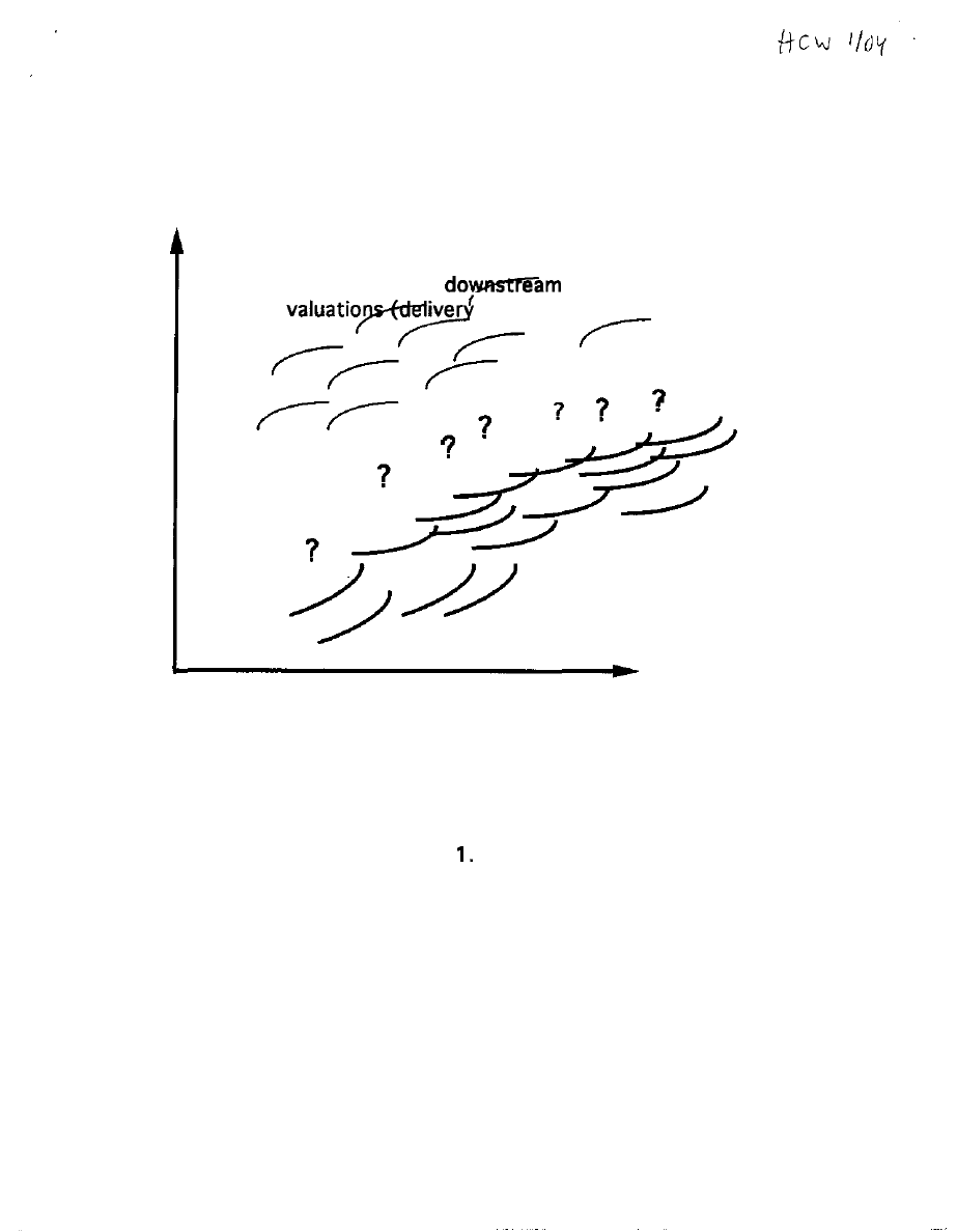
money valuations
fuzz of possible
side)
fuzz of possible upstream
valuations (cost side)
y
volume
Figure
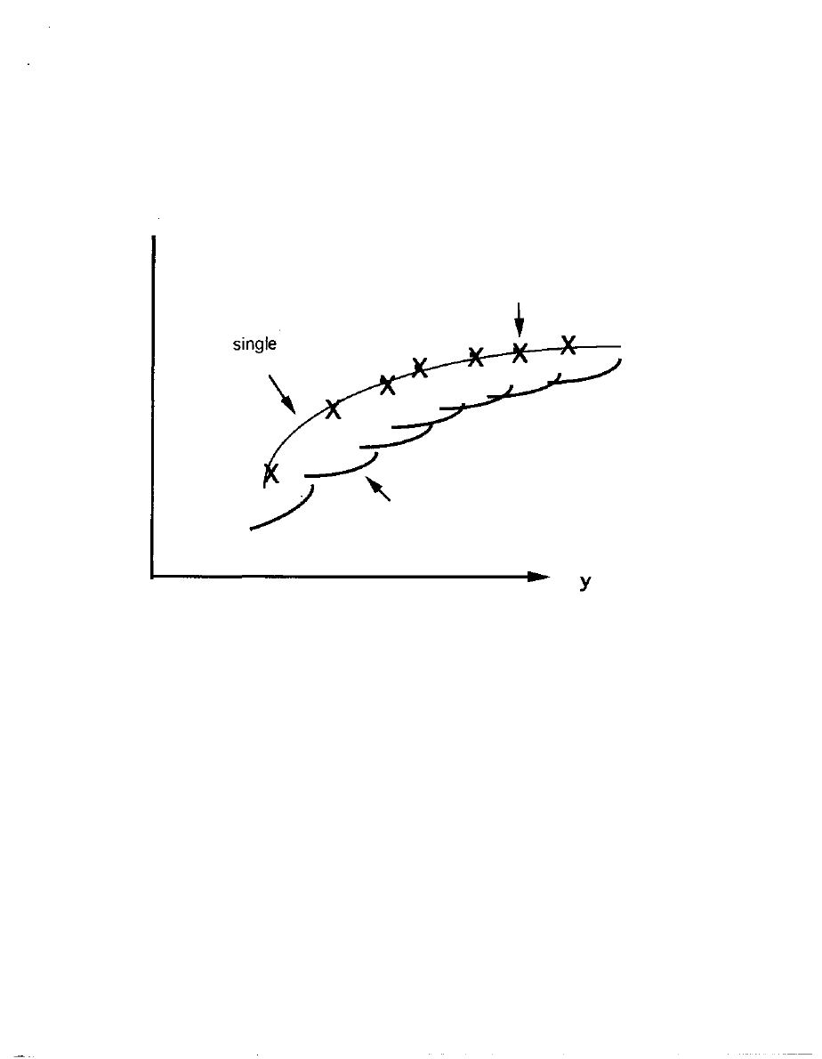
revenue W(y)
cost C(y;n)
t
the
market profile
revenue, volume
for producer 6
cost schedule for producer 2
volume
Figure 2.
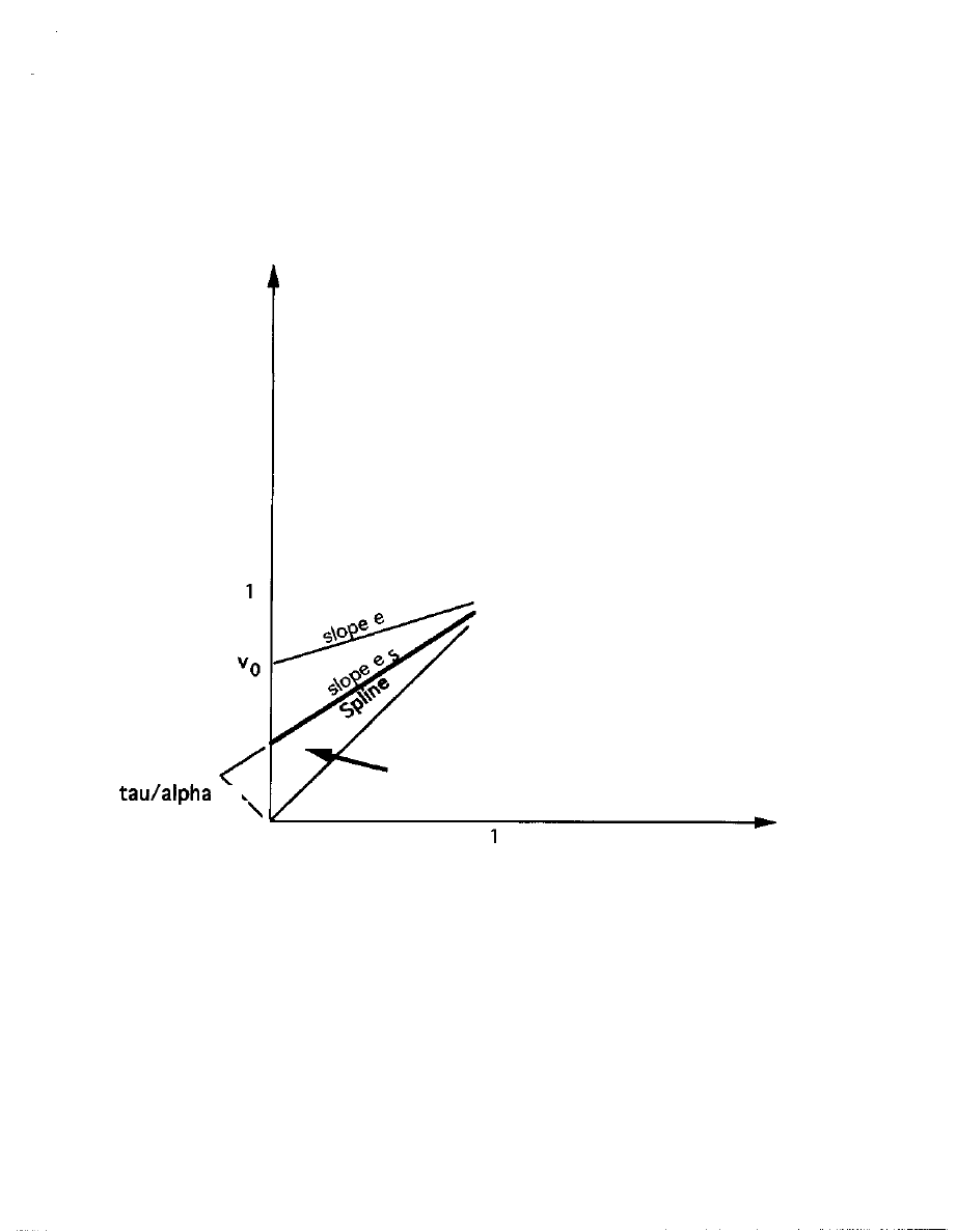
a/c volume
tradeoff = v
height =
ORDINARY
b/d quality
tradeoff = u
Figure 3
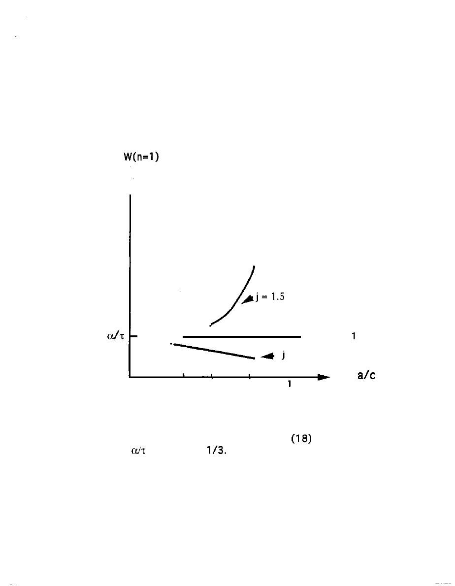
t
q
• Spline : j =
= 0.7
0.33 0.5 0.75
V =
Figure 4. Variation of revenue for lowest cost
producer on each of three rays: eq
with
taken to be
Each curve terminates on
the left at the p.c. v for that ray.
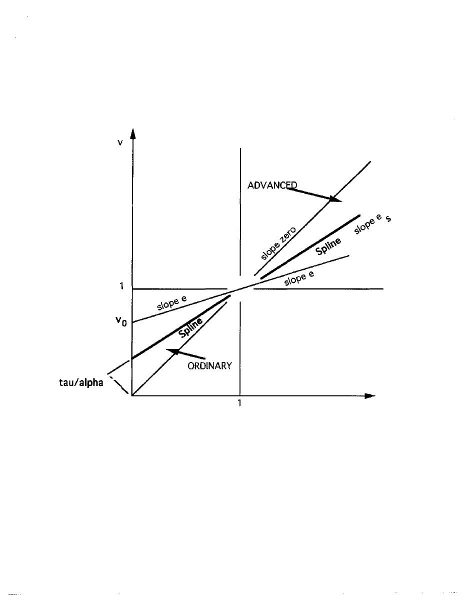
a/c volume
tradeoff =
height =
b/d quality
tradeoff = u
Figure 5
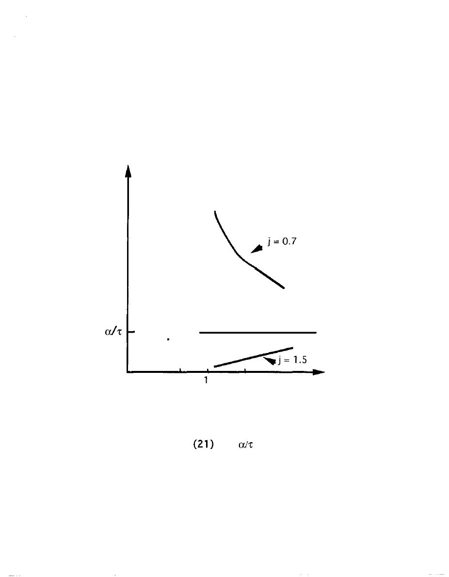
W(n=l)
q
Spline : j = 1
v = a/c
1.5
Figure 6. ADVANCED region: Variation of
revenue for lowest cost producer on each of
three rays: eq
with
taken to be 1/3.
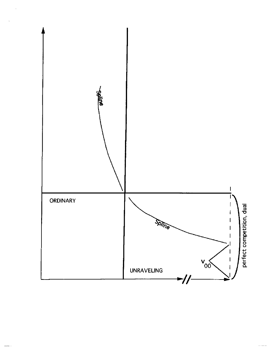
v= c/a
(consult equations 26 and 25 and 24)
TRUSTS
ADVANCED
u=d/b
Figure 7. Parabolic rays for growth in revenue, with
upstream orientation, from dual perfect competition
-state space analogous to Figure 5.
u=00
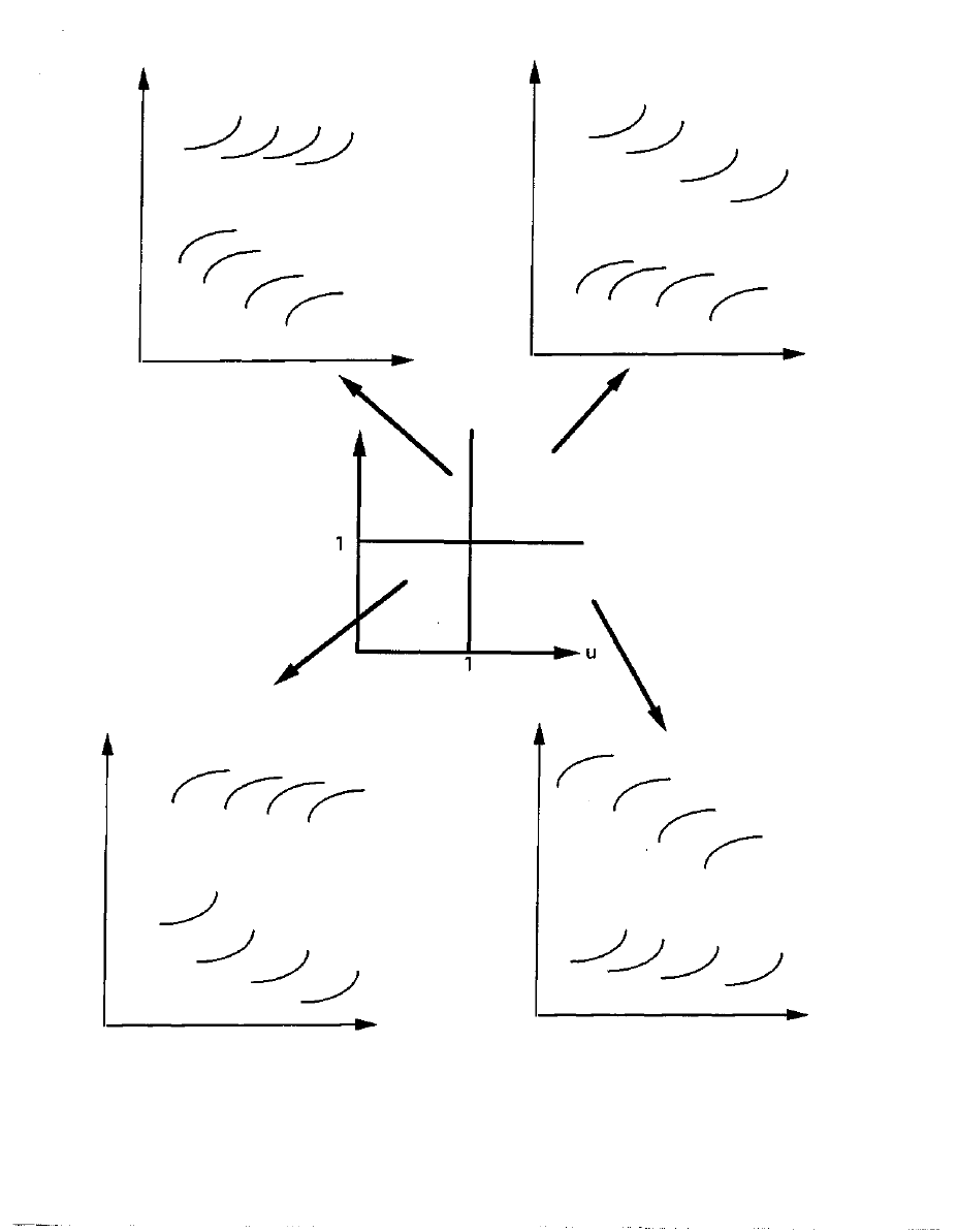
dollars
valuations
costs
dollars
valuations
costs
volume
volume
v
dollars
dollars
valuations
costs
valuations
costs
volume
volume
Figure 8 Contrasts, by quadrant of state space, between curvatures of
monetary schedules and their vertical displacements by quality
of producers (four for illustration)
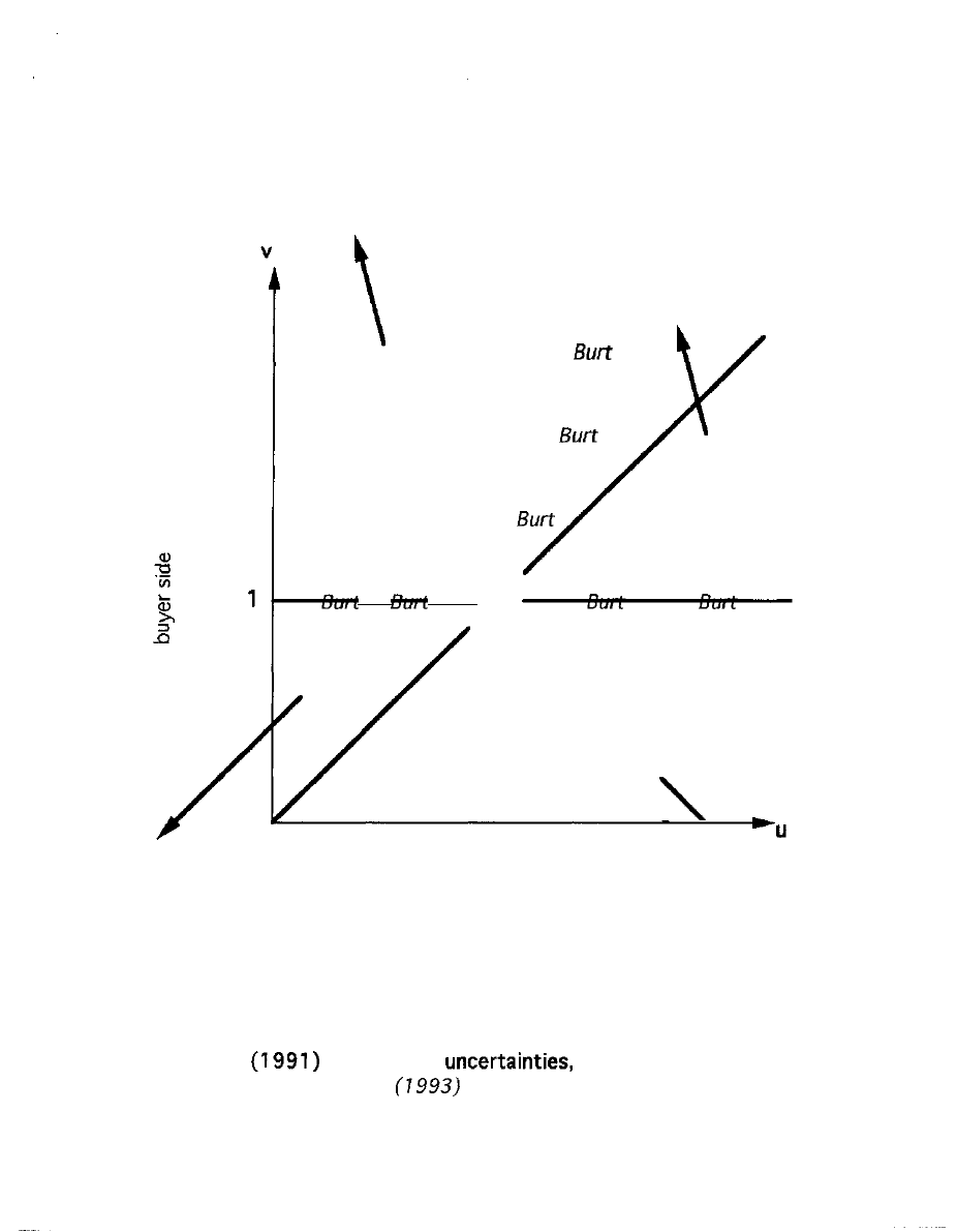
TRUSTS
ORDINARY
ADVANCED
[HIGH, LOW]
[HIGH, HIGH]
Burt
[LOW,LOW]
Burt
[LOW, HIGH]
Burt
Burt
1
producer side
\
UNRAVELING
2x2 table entries:
[BUYER SIDE UNCERTAINTY, PRODUCER SIDE UNCERTAINTY]
Figure 9. Market state space seen as Podolny
2x2 table of
with interleaved
borders of Burt
manipulation
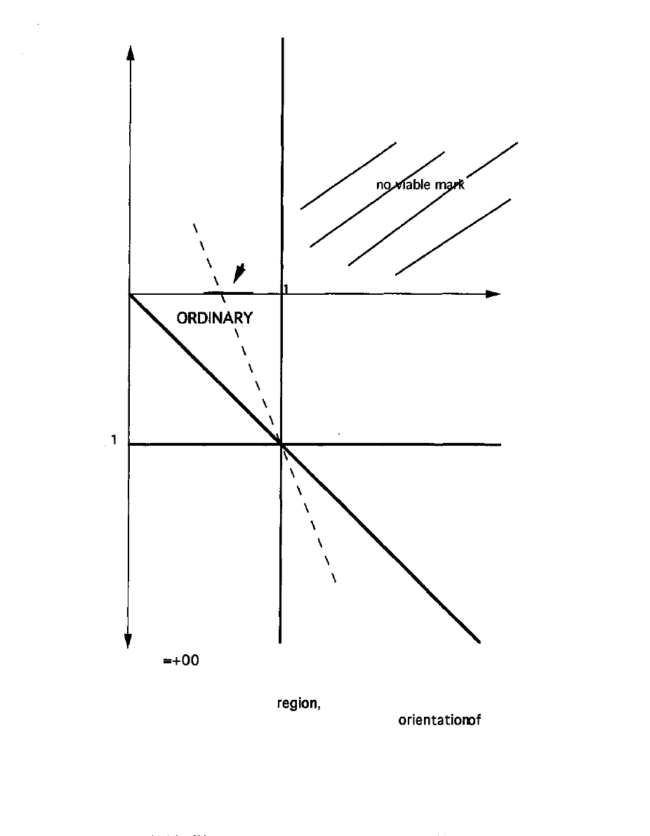
u = -00
0
PARADOX
p.c.
et solutions
ADVANCED
u = b/d
v = a/c
Figure 10. PARADOX
for negative values of u,
adjoined to state space for downstream
Fig. 5 (rotated by 90, abd showing the illustrative ray extended)
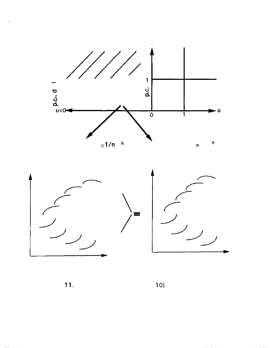
V
re
3
PARADOX
upstream: W(n)
downstream: W(n) n
dollars
dollars
valuations
costs
valuations
costs
volume
volume
Figure
For PARADOX region (see Fig.
contrasts between the
curvatures of monetary schedules and their vertical displacements by
quality, for orientations upstream and down
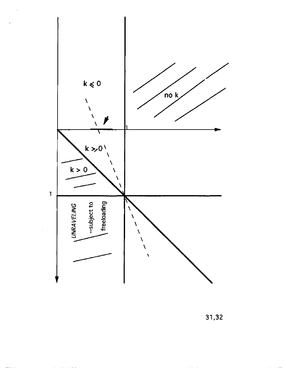
0
PARADOX
p.c.
ORDINARY
k > 0
[TRUSTS]
k > 0
k> 0
any
k
ADVANCED
u = b/d
v = a/c
Figure 12. Allowed range of solutions for W(y),
by region for downstream orientation: consult eqs
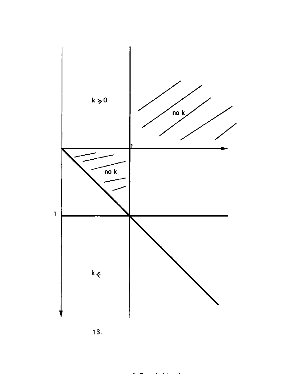
0
PARADOX
k<0
UNRAVELING
0
u =
d/b
TRUSTS
any
k
any
k
k<0
v = c/a
Figure
Allowed range of solutions for W(y), by region
for upstream orientation
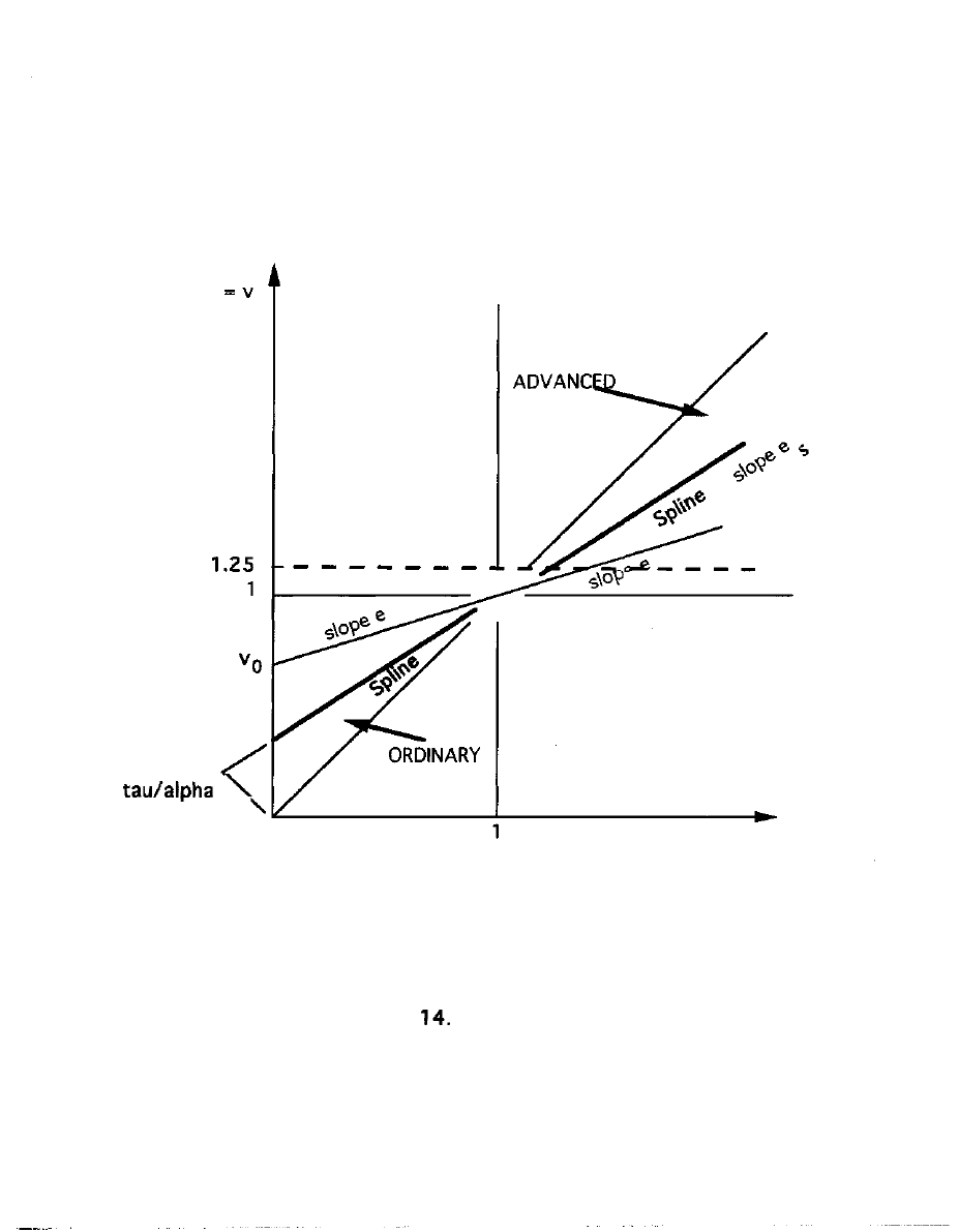
a/c volume
tradeoff
height =
CROWDED
b/d quality
tradeoff = u
Figure
Crowded band
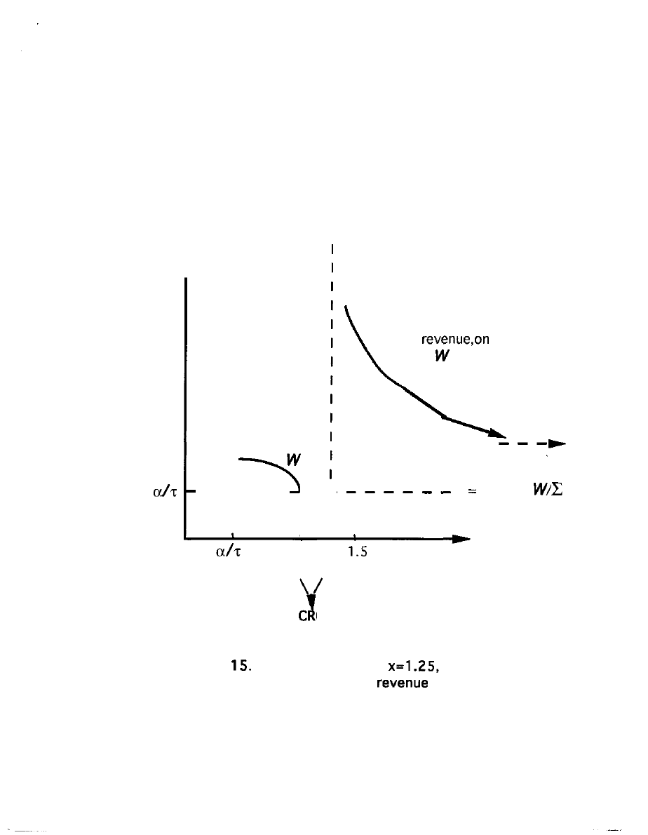
revenue
t
q
aggregate market
Spline
0
[Spline
]
v = a/c
1 x
1.25
OWDED BAND
Figure
With substitutability
variation of aggregate market
W
along Spline, downstream orientation

Recent ISERP Working Papers
04-01: “Reducing Bias in Treatment Effect Estimation in Observational Studies Suffering from
Missing Data,” Jennifer Hill, International and Public Affairs, Columbia University
03-01: “The Plasticity of Participation: Evidence From a Participatory Governance Experiment,”
Shubham Chaudhuri, Economics, Columbia University, and Patrick Heller, Sociology, Brown
University
03-02: “Factional Politics and Credit Networks in Revolutionary Vermont,” Henning Hillmann,
Sociology, Columbia University
03-03 “ ‘Active Patients’ in Rural African Health Care: Implications for Welfare, Policy and
Privatization,” Kenneth L. Leonard, Economics, Columbia University
03-04 “Living at the Edge: America’s Low-Income Children and Families,” Hsien-Hen Lu, Public
Health, Columbia University, Julian Palmer, Younghwan Song, Economics, Union College, Mary
Clare Lennon, Public Health, Columbia University, Lawrence Aber, Public Health, Columbia
University
02-02 “Substitutability Cross-Stream Between Oriented Markets: Conventions in the Wine Sector of
France,” Harrison White, Sociology, Columbia University
02-03 “Link, Search, Interact: The Co-Evolution of NGOs and Interactive Technology,” Jonathan
Bach, Center on Organizational Innovation, Columbia University and David Stark, Center on
Organizational Innovation, Columbia University
02-04 “Chains of Affection: The Structure of Adolescent Romantic and Sexual Networks,” Peter
Bearman, Institute for Social and Economic Research and Policy, Columbia University, James
Moody, Sociology, Ohio State, Katherine Stovel, Sociology, University of Washington
02-05 “Permanently Beta: Responsive Organization in the Internet Era,” Gina Neff, Center on
Organizational Innovation (COI), Columbia University, and David Stark, Center on Organizational
Innovation (COI), Columbia University
02-06 “Negotiating the End of Transition: A Network Approach to Political Discourse Dynamics,
Hungary 1997,” Balázs Vedres, Columbia University, Péter Csigó, Ecole des Hautes Etudes en
Sciences Sociales
For copies of ISERP Working Papers
visit http://www.iserp.columbia.edu/initiatives/working_papers/paper_program.html,
write to iserp@columbia.edu or call 212-854-3081

E
DITORIAL
B
OARD
Karen Barkey, Sociology
Peter Bearman, Sociology/
ISERP
Alan Brinkley, History
Charles Cameron, Political Science
Alessandra Casella, Economics
Ester Fuchs, Political Science/
SIPA
John Huber, Political Science
Ira Katznelson, Political Science/History
Herbert Klein, History
Mary Clare Lennon, Public Health
Mahmood Mamdani, Anthropology
Marianthi Markatou, Statistics
William McAllister,
ISERP
Kathryn Neckerman,
ISERP
Richard Nelson, Business/
SIPA
Elliot Sclar, Architecture, Planning and
Preservation/
SIPA
Seymour Spilerman, Sociology
Charles Tilly, Sociology
Harrison White, Sociology
A
DMINISTRATION
Peter Bearman, Director
Kathryn Neckerman, Associate Director
Leslie Wright, Assistant Director
Institute for Social and Economic
Research and Policy
Columbia University
International Affairs Building
420 West 118 Street, 8
th
Floor
Mail Code 3355
New York, NY 10027
telephone: 212-854-3081
facsimile: 212-854-8925
e-mail: iserp@columbia.edu
URL
: http://www.iserp.columbia.edu
Document Outline
- 04-02 White front cover.pdf
Wyszukiwarka
Podobne podstrony:
więcej podobnych podstron