
Quantum Field Theory
Part II: Spin One Half
Mark Srednicki
Department of Physics
University of California
Santa Barbara, CA 93106
mark@physics.ucsb.edu
This is a draft version of Part II of a three-part textbook on quantum field
theory.
1

Part II: Spin One Half
33) Representations of the Lorentz Group (2)
34) Left- and Right-Handed Spinor Fields (3, 33)
35) Manipulating Spinor Indices (34)
36) Lagrangians for Spinor Fields (4, 22, 35)
37) Canonical Quantization of Spinor Fields I (36)
38) Spinor Technology (37)
39) Canonical Quantization of Spinor Fields II (38)
40) Parity, Time Reversal, and Charge Conjugation (39)
41) LSZ Reduction for Spin-One-Half Particles (39)
42) The Free Fermion Propagator (39)
43) The Path Integral for Fermion Fields (9, 42)
44) Formal Development of Fermionic Path Integrals (43)
45) The Feynman Rules for Dirac Fields and Yukawa Theory (10, 13, 41,
43)
46) Spin Sums (45)
47) Gamma Matrix Technology (36)
48) Spin-Averaged Cross Sections in Yukawa Theory (46, 47)
49) The Feynman Rules for Majorana Fields (45)
50) Massless Spin-One-Half Particles and Spinor Helicity (48)
51) Loop Corrections in Yukawa Theory (19, 40, 48)
52) Beta Functions in Yukawa Theory (27, 51)
53) Functional Determinants (44, 45)
2

Quantum Field Theory
Mark Srednicki
33: Representations of the Lorentz Group
Prerequisite: 2
In section 2, we saw that we could define a unitary operator U(Λ) that
implemented a Lorentz transformation on a scalar field ϕ(x) via
U(Λ)
−1
ϕ(x)U(Λ) = ϕ(Λ
−1
x) .
(1)
As shown in section 2, this implies that the derivative of the field transforms
as
U(Λ)
−1
∂
µ
ϕ(x)U(Λ) = Λ
µ
ρ
¯
∂
ρ
ϕ(Λ
−1
x) ,
(2)
where the bar on he derivative means that it is with respect to the argument
¯
x = Λ
−1
x.
Eq. (2) suggests that we could define a vector field A
µ
(x) which would
transform as
U(Λ)
−1
A
ρ
(x)U(Λ) = Λ
µ
ρ
A
ρ
(Λ
−1
x) ,
(3)
or a tensor field B
µν
(x) which would transform as
U(Λ)
−1
B
µν
(x)U(Λ) = Λ
µ
ρ
Λ
ν
σ
B
ρσ
(Λ
−1
x) .
(4)
Note that if B
µν
is either symmetric, B
µν
(x) = B
νµ
(x), or antisymmetric,
B
µν
(x) =
−B
νµ
(x), then this symmetry property is preserved by the Lorentz
transformation. Also, if we take the trace to get T (x)
≡ g
µν
B
µν
(x), then,
using g
µν
Λ
µ
ρ
Λ
ν
σ
= g
ρσ
, we find that T (x) transforms like a scalar field,
U(Λ)
−1
T (x)U(Λ) = T (Λ
−1
x) .
(5)
Thus, given a tensor field B
µν
(x) with no particular symmetry, we can write
B
µν
(x) = A
µν
(x) + S
µν
(x) +
1
4
g
µν
T (x) ,
(6)
3

where A
µν
is antisymmetric (A
µν
=
−A
νµ
) and S
µν
is symmetric (S
µν
= S
νµ
)
and traceless (g
µν
S
µν
= 0). The key point is that the fields A
µν
, S
µν
, and T
do not mix with each other under Lorentz transformations.
Is it possible to further break apart these fields into still smaller sets that
do not mix under Lorentz transformations? How do we make this decomposi-
tion into irreducible representations of the Lorentz group for a field carrying
n vector indices? Are there any other kinds of indices we could consistently
assign to a field? If so, how do these behave under a Lorentz transformation?
The answers to these questions are to be found in the theory of group
representations
. Let us see how this works for the Lorentz group in four
spacetime dimensions.
For an infinitesimal transformation Λ
µ
ν
= δ
µ
ν
+ δω
µ
ν
, we can write
U(1+δω) = I +
i
2
δω
µν
M
µν
,
(7)
where M
µν
=
−M
νµ
is a set of hermitian operators, the generators of the
Lorentz group
. As shown in section 2, these obey the commutation relations
[M
µν
, M
ρσ
] = i
g
µρ
M
νσ
− (µ↔ν)
− (ρ↔σ) .
(8)
We can identify the components of the angular momentum operator ~
J as
J
i
≡
1
2
ε
ijk
M
jk
and the components of the boost operator ~
K as K
i
≡ M
i0
.
We then find from eq. (8) that
[J
i
, J
j
] = +iε
ijk
J
k
,
(9)
[J
i
, K
j
] = +iε
ijk
K
k
,
(10)
[K
i
, K
j
] =
−iε
ijk
J
k
.
(11)
We would now like to find all the representations of eqs. (9–11). A repre-
sentation is a set of finite-dimensional matrices with the same commutation
relations. For example, if we restrict our attention to eq. (9) alone, we know
(from standard results in the quantum mechanics of angular momentum)
that we can find three (2j+1)
× (2j+1) hermitian matrices J
1
,
J
2
, and
J
3
that obey eq. (9), and that the eigenvalues of (say)
J
3
are
−j, −j+1, . . . , +j,
where j has the possible values 0,
1
2
, 1, . . . . We further know that these ma-
trices constitute all of the inequivalent, irreducible representations of SO(3),
4

the rotation group in three dimensions. (Inequivalent means not related by
a unitary transformation; irreducible means cannot be made block-diagonal
by a unitary transformation.) We would like to extend these conclusions to
encompass the full set of eqs. (9–11).
In order to do so, it is helpful to define some nonhermitian operators
whose physical significance is obscure, but which simplify the commutation
relations. These are
N
i
≡
1
2
(J
i
− iK
i
) ,
(12)
N
†
i
≡
1
2
(J
i
+ iK
i
) .
(13)
In terms of N
i
and N
†
i
, eqs. (9–11) become
[N
i
, N
j
] = iε
ijk
N
k
,
(14)
[N
†
i
, N
†
j
] = iε
ijk
N
†
k
,
(15)
[N
i
, N
†
j
] = 0 .
(16)
We recognize these as the commutation relations of two independent SO(3)
groups [or, equivalently, SU(2); see section 32]. Thus the Lorentz group in
four dimensions is equivalent to SO(3)
×SO(3). And, as just discussed, we
are already familiar with the representation theory of SO(3). We therefore
conclude that the representations of the Lorentz group in four spacetime
dimensions are specified by two numbers n and n
′
, each a nonnegative integer
or half-integer.
This turns out to be correct, but there is a complication. To derive the
usual representation theory of SO(3), as is done in any text on quantum
mechanics, we need to use the fact that the components J
i
of the angular
momentum operator are hermitian. The components N
i
of eq. (13), on the
other hand, are not. This means that we have to redo the usual derivation
of the representations of SO(3), and see what changes.
As we have already noted, the final result is the naive one, that the
representations of the Lorentz group in four dimensions are the same as the
representations of SO(3)
×SO(3). Those uninterested in the (annoyingly com-
plicated) details can skip ahead all the way ahead to the last four paragraphs
of this section.
5

We begin by noting that ~
N
2
commutes with N
i
; this is easily derived
from eq. (14). Similarly, ~
N
†2
commutes with N
†
i
. Eq. (16) then implies that
~
N
2
, N
3
, ~
N
†2
, and N
†
3
are all mutually commuting. Therefore, we can define
a set of simultaneous eigenkets
|n, m; n
′
, m
′
i, where the eigenvalues of ~
N
2
,
N
3
, ~
N
†2
, and N
†
3
are f (n), m, f (n
′
), and m, respectively. [Later we will
see that n and n
′
must be nonnegative integers or half-integers, and that
f (n) = n(n+1), as expected.] We also define a set of bra states
hn, m; n
′
, m
′
|
that, by definition, obey
hn
2
, m
2
; n
′
2
, m
′
2
|n
1
, m
1
; n
′
1
, m
′
1
i = δ
n2n1
δ
m2m1
δ
n
′
2
n
′
1
δ
m
′
2
m
′
1
≡ ∆
21
(17)
and
X
|n, m; n
′
, m
′
ihn, m; n
′
, m
′
| = 1 .
(18)
In eq. (18), the sum is over all allowed values of n, m, n
′
, and m
′
; our goal is
to determine these allowed values.
From the discussion so far, we can conclude that
hn
2
, m
2
; n
′
2
, m
′
2
| ~
N
2
|n
1
, m
1
; n
′
1
, m
′
1
i = f(n
1
) ∆
21
,
(19)
hn
2
, m
2
; n
′
2
, m
′
2
| N
3
|n
1
, m
1
; n
′
1
, m
′
1
i =
m
1
∆
21
,
(20)
hn
2
, m
2
; n
′
2
, m
′
2
| ~
N
†2
|n
1
, m
1
; n
′
1
, m
′
1
i = f(n
′
1
) ∆
21
,
(21)
hn
2
, m
2
; n
′
2
, m
′
2
| N
3
|n
1
, m
1
; n
′
1
, m
′
1
i =
m
′
1
∆
21
.
(22)
Note that we have not yet made any assumptions about the properties of
the states under hermitian conjugation. From eqs. (14) and (15), we see that
hermitian conjugation exchanges the two SO(3) groups. Therefore, we must
have
|n, m; n
′
, m
′
i
†
=
hn
′
, m
′
; n, m
| ,
(23)
hn, m; n
′
, m
′
|
†
=
|n
′
, m
′
; n, m
i ,
(24)
up to a possible phase factor that turns out to be irrelevant. Compare the
ordering of the labels in eqs. (23) and (24) with those in eqs. (17) and (18); a
state
|n, m; n
′
, m
′
i has zero inner product with its own hermitian conjugate
if n
6= n
′
or m
6= m
′
.
6

Next, take the hermitian conjugates of eqs. (19) and (20), using eqs. (23)
and (24). We get
hn
′
1
, m
′
1
; n
1
, m
1
| ~
N
†2
|n
′
2
, m
′
2
; n
2
, m
2
i = [f(n
1
)]
∗
∆
21
,
(25)
hn
′
1
, m
′
1
; n
1
, m
1
| N
†
3
|n
′
2
, m
′
2
; n
2
, m
2
i =
m
∗
1
∆
21
,
(26)
Comparing eqs. (25) and (26) with eqs. (21) and (22), we find that the allowed
values of f (n) and m are real.
We now define the raising and lowering operators
N
±
≡ N
1
± iN
2
,
(27)
(N
†
)
±
≡ N
†
1
± iN
†
2
;
(28)
note that
(N
±
)
†
= (N
†
)
∓
.
(29)
The commutation relations (14) become
[N
3
, N
±
] =
±N
±
,
(30)
[N
+
, N
−
] = 2N
3
,
(31)
plus the equivalent with N
→ N
†
. By inserting a complete set of states
into eq. (30), and mimicking the usual procedure in quantum mechanics, it
is possible to show that
hn
2
, m
2
+1; n
′
2
, m
′
2
| N
+
|n
1
, m
1
; n
′
1
, m
′
1
i = λ
+
(n
1
, m
1
) ∆
21
,
(32)
hn
1
, m
1
; n
′
1
, m
′
1
| N
−
|n
2
, m
2
+1; n
′
2
, m
′
2
i = λ
−
(n
1
, m
1
) ∆
21
,
(33)
where λ
+
(n, m) and λ
−
(n, m) are functions to be determined. By inserting
a complete set of states into eq. (31), and using eqs. (32) and (33), we can
show that
λ
+
(n, m
−1)λ
−
(n, m
−1) − λ
+
(n, m)λ
−
(n, m) = 2m .
(34)
The solution of this recursion relation is
λ
+
(n, m)λ
−
(n, m) = C(n)
− m(m+1) ,
(35)
7

where C(n) is an arbitrary function of n.
Next we need the parity operator P , introduced in section 23. From the
discussion there, we can conclude that
P
−1
M
µν
P =
P
µ
ρ
P
ν
σ
M
ρσ
,
(36)
where
P
µ
ν
=
+1
−1
−1
−1
.
(37)
Eq. (36) implies
P
−1
J
i
P = +J
i
,
(38)
P
−1
K
i
P =
−K
i
,
(39)
or, equivalently,
P
−1
N
i
P = N
†
i
,
(40)
P
−1
N
†
i
P = N
i
.
(41)
Since P exchanges N
i
and N
†
i
, it must be that
P
|n, m; n
′
, m
′
i = |n
′
, m
′
; n, m
i ,
(42)
P
−1
|n, m; n
′
, m
′
i = |n
′
, m
′
; n, m
i ,
(43)
up to a possible phase factor that turns out to be irrelevant. Taking the
hermitian conjugate of eqs. (42) and (43), we get
hn
′
, m
′
; n, m
|P
−1
=
hn, m; n
′
, m
′
| ,
(44)
hn
′
, m
′
; n, m
|P
=
hn, m; n
′
, m
′
| ,
(45)
where we have used the fact that P is unitarity: P
†
= P
−1
.
Now we can take eq. (32) and insert P P
−1
on either side of N
+
to get
λ
+
(n
1
, m
1
) ∆
21
=
hn
2
, m
2
+1; n
′
2
, m
′
2
| P P
−1
N
+
P P
−1
|n
1
, m
1
; n
′
1
, m
′
1
i
=
hn
′
2
, m
′
2
; n
2
, m
2
+1
| P
−1
N
+
P
|n
′
1
, m
′
1
; n
1
, m
1
i
=
hn
′
2
, m
′
2
; n
2
, m
2
+1
| (N
†
)
+
|n
′
1
, m
′
1
; n
1
, m
1
i .
(46)
8

In the second line, we used eqs. (43) and (45). In the third, we used eq. (40).
Now taking the hermitian conjugate of eq. (46), and using eqs. (23), (24), and
(29), we find
hn
1
, m
1
; n
′
1
, m
′
1
| N
−
|n
2
, m
2
+1; n
′
2
, m
′
2
i = [λ
+
(n
1
, m
1
)]
∗
∆
21
.
(47)
Comparing eq. (47) with eq. (33), we see that
λ
−
(n, m) = [λ
+
(n, m)]
∗
.
(48)
This is the final ingredient. Putting eq. (48) into eq. (35), we get
|λ
+
(n, m)
|
2
= C(n)
− m(m+1) .
(49)
From here, everything can be done by mimicking the usual procedure in the
quantum mechanics of angular momentum. We see that the left-hand side of
eq. (49) is real and nonnegative, while the right-hand side becomes negative
for sufficiently large
|m|. This is not a problem if there are two values of
m, differing by an integer, for which λ
+
(n, m) is zero. From this we can
deduce that the allowed values of m are real integers or half-integers, and
that if we choose C(n) = n(n+1), then n is an integer or half-integer such
that the allowed values of m are
−n, −n+1, . . . , +n. We can also show that
f (n) = C(n) = n(n+1). Thus the representations of the Lorentz group in
four dimensions are just the same as those of SO(3)
×SO(3).
We will label these representations as (2n+1, 2n
′
+1); the number of com-
ponents of a representation is then (2n+1)(2n
′
+1). Different components
within a representation can also be labeled by their angular momentum rep-
resentations. To do this, we first note that, from eqs. (12) and (13), we have
~
J = ~
N + ~
N
†
. Thus, deducing the allowed values of j given n and n
′
becomes
a standard problem in the addition of angular momenta. The general result
is that the allowed values of j are
|n−n
′
|, |n−n
′
|+1, . . . , n+n
′
, and each of
these values appears exactly once.
The four simplest and most often encountered representations are (1, 1),
(2, 1), (1, 2), and (2, 2). These are given special names:
(1, 1) = Scalar or singlet
9

(2, 1) = Left-handed spinor
(1, 2) = Right-handed spinor
(2, 2) = Vector
(50)
It may seem a little surprising that (2, 2) is to be identified as the vector rep-
resentation. To see that this must be the case, we first note that the vector
representation is irreducible: all the components of a four-vector mix with
each other under a general Lorentz transformation. Secondly, the vector rep-
resentation has four components. Therefore, the only candidate irreducible
representations are (4, 1), (1, 4), and (2, 2). The first two of these contain
angular momenta j =
3
2
only, whereas (2, 2) contains j = 0 and j = 1. This
is just right for a four-vector, whose time component is a scalar under spatial
rotations, and whose space components are a three-vector.
In order to gain a better understanding of what it means for (2, 2) to be
the vector representation, we must first investigate the spinor representations
(1, 2) and (2, 1), which contain angular momenta j =
1
2
only.
Problems
33.1) Express A
µν
(x), S
µν
(x), and T (x) in terms of B
µν
(x).
33.2) Verify that eqs. (14–16) follow from eqs. (9–11).
10

Quantum Field Theory
Mark Srednicki
34: Left- and Right-Handed Spinor Fields
Prerequisite: 33
Consider a left-handed spinor field ψ
a
(x), also known as a left-handed
Weyl field
, which is in the (2, 1) representation of the Lorentz group. Here
the index a is a left-handed spinor index that takes on two possible values.
Under a Lorentz transformation, we have
U(Λ)
−1
ψ
a
(x)U(Λ) = L
a
b
(Λ)ψ
b
(Λ
−1
x) ,
(51)
where L
a
b
(Λ) is a matrix in the (2, 1) representation. These matrices satisfy
the group composition rule
L
a
b
(Λ
1
)L
b
c
(Λ
2
) = L
a
c
(Λ
1
Λ
2
) .
(52)
For an infinitesimal transformation Λ
µ
ν
= δ
µ
ν
+ δω
µ
ν
, we can write
L
a
b
(1+δω) = δ
a
b
+
i
2
δω
µν
(S
µν
L
)
a
b
,
(53)
where (S
µν
L
)
a
b
=
−(S
νµ
L
)
a
b
is a set of 2
× 2 matrices that obey the same
commutation relations as the generators M
µν
, namely
[S
µν
L
, S
ρσ
L
] = i
g
µρ
S
νσ
L
− (µ↔ν)
− (ρ↔σ) .
(54)
Using
U(1+δω) = I +
i
2
δω
µν
M
µν
,
(55)
eq. (51) becomes
[ψ
a
(x), M
µν
] =
−i(x
µ
∂
ν
−x
ν
∂
µ
)ψ
a
(x) + (S
µν
L
)
a
b
ψ
b
(x) .
(56)
The first term on the right-hand side of eq. (56) would also be present for
a scalar field, and is not the focus of our current interest; we will suppress
11

it by evaluating the fields at the spacetime origin, x
µ
= 0. Recalling that
M
ij
= ε
ijk
J
k
, where J
k
is the angular momentum operator, we have
ε
ijk
[ψ
a
(0), J
k
] = (S
ij
L
)
a
b
ψ
b
(0) .
(57)
Recall that the (2, 1) representation of the Lorentz group includes angular
momentum j =
1
2
only. For a spin-one-half operator, the standard convention
is that the matrix on the right-hand side of eq. (57) is
1
2
ε
ijk
σ
k
, where σ
k
is a
Pauli matrix:
σ
1
=
0 1
1 0
,
σ
2
=
0
−i
i
0
,
σ
3
=
1
0
0
−1
.
(58)
We therefore conclude that
(S
ij
L
)
a
b
=
1
2
ε
ijk
σ
k
.
(59)
Thus, for example, setting i=1 and j=2 yields (S
12
L
)
a
b
=
1
2
ε
12k
σ
k
=
1
2
σ
3
,
where the subscript a is the row index (and the superscript b is the column
index) of the matrix
1
2
σ
3
. Therefore, (S
12
L
)
1
1
= +
1
2
, (S
12
L
)
2
2
=
−
1
2
, and
(S
12
L
)
1
2
= (S
12
L
)
2
1
= 0.
Once we have the (2, 1) representation matrices for the angular momen-
tum operator J
i
, we can easily get them for the boost operator K
k
= M
k0
.
This is because J
k
= N
k
+ N
†
k
and K
k
= i(N
k
− N
†
k
), and, in the (2, 1)
representation, N
†
k
is zero. Therefore, the representation matrices for K
k
are
simply i times those for J
k
, and so
(S
k0
L
)
a
b
=
1
2
iσ
k
.
(60)
Now consider taking the hermitian conjugate of the left-handed spinor
field ψ
a
(x). Recall that hermitian conjugation swaps the two SO(3) factors
in the Lorentz group. Therefore, the hermitian conjugate of a field in the
(2, 1) representation should be a field in the (1, 2) representation; such a field
is called a right-handed spinor field, or a right-handed Weyl field. We will
distinguish the indices of the (1, 2) representation from those of the (2, 1)
representation by putting dots over them. Thus, we write
[ψ
a
(x)]
†
= ψ
†
˙a
(x) .
(61)
12

Under a Lorentz transformation, we have
U(Λ)
−1
ψ
†
˙a
(x)U(Λ) = R
˙a
˙b
(Λ)ψ
†
˙b
(Λ
−1
x) ,
(62)
where R
˙a
˙b
(Λ) is a matrix in the (1, 2) representation. These matrices satisfy
the group composition rule
R
˙a
˙b
(Λ
1
)R
˙b
˙c
(Λ
2
) = R
˙a
˙c
(Λ
1
Λ
2
) .
(63)
For an infinitesimal transformation Λ
µ
ν
= δ
µ
ν
+ δω
µ
ν
, we can write
R
˙a
˙b
(1+δω) = δ
˙a
˙b
+
i
2
δω
µν
(S
µν
R
)
˙a
˙b
,
(64)
where (S
µν
R
)
˙a
˙b
=
−(S
νµ
R
)
˙a
˙b
is a set of 2
× 2 matrices that obey the same
commutation relations as the generators M
µν
. We then have
[ψ
†
˙a
(0), M
µν
] = (S
µν
R
)
˙a
˙b
ψ
†
˙b
(0) .
(65)
Taking the hermitian conjugate of this equation, we get
[M
µν
, ψ
a
(0)] = [(S
µν
R
)
˙a
˙b
]
∗
ψ
b
(0) .
(66)
Comparing this with eq. (56), we see that
(S
µν
R
)
˙a
˙b
=
−[(S
µν
L
)
a
b
]
∗
.
(67)
In the previous section, we examined the Lorentz-transformation proper-
ties of a field carrying two vector indices. To help us get better acquainted
with the properties of spinor indices, let us now do the same for a field that
carries two (2, 1) indices. Call this field C
ab
(x). Under a Lorentz transfor-
mation, we have
U(Λ)
−1
C
ab
(x)U(Λ) = L
a
c
(Λ)L
b
d
(Λ)C
cd
(Λ
−1
x) .
(68)
The question we wish to address is whether or not the four components of
C
ab
can be grouped into smaller sets that do not mix with each other under
Lorentz transformations.
To answer this question, recall from quantum mechanics that two spin-
one-half particles can be in a state of total spin zero, or total spin one.
13

Furthermore, the single spin-zero state is the unique antisymmetric combi-
nation of the two spin-one-half states, and the three spin-one states are the
three symmetric combinations of the two spin-one-half states. We can write
this schematically as 2
⊗ 2 = 1
A
⊕ 3
S
, where we label the representation of
SO(3) by the number of its components, and the subscripts S and A indi-
cate whether that representation appears in the symmetric or antisymmetric
combination of the two 2’s. For the Lorentz group, the relevant relation is
(2, 1)
⊗ (2, 1) = (1, 1)
A
⊕ (3, 1)
S
. This implies that we should be able to write
C
ab
(x) = ε
ab
D(x) + G
ab
(x) ,
(69)
where D(x) is a scalar field, ε
ab
=
−ε
ba
is an antisymmetric set of constants,
and G
ab
(x) = G
ba
(x). The symbol ε
ab
is uniquely determined by its symmetry
properties up to an overall constant; we will choose ε
21
=
−ε
12
= +1.
Given that D(x) is a Lorentz scalar, eq. (69) is consistent with eq. (68)
only if
L
a
c
(Λ)L
b
d
(Λ)ε
cd
= ε
ab
.
(70)
This means that ε
ab
is an invariant symbol of the Lorentz group: it does not
change under a Lorentz transformation that acts on all of its indices. In this
way, ε
ab
is analogous to the metric g
µν
, which is also an invariant symbol,
since
Λ
µ
ρ
Λ
ν
σ
g
ρσ
= g
µν
.
(71)
We use g
µν
and its inverse g
µν
to raise and lower vector indices, and we can
use ε
ab
and and its inverse ε
ab
to raise and lower left-handed spinor indices.
Here we define ε
ab
via
ε
12
= ε
21
= +1 ,
ε
21
= ε
12
=
−1 .
(72)
With this definition, we have
ε
ab
ε
bc
= δ
a
c
,
ε
ab
ε
bc
= δ
a
c
.
(73)
We can then define
ψ
a
(x)
≡ ε
ab
ψ
b
(x) .
(74)
We also have (suppressing the spacetime argument of the field)
ψ
a
= ε
ab
ψ
b
= ε
ab
ε
bc
ψ
c
= δ
a
c
ψ
c
,
(75)
14

as we would expect. However, the antisymmetry of ε
ab
means that we must
be careful with minus signs; for example, eq. (74) can be written in various
ways, such as
ψ
a
= ε
ab
ψ
b
=
−ε
ba
ψ
b
=
−ψ
b
ε
ba
= ψ
b
ε
ab
.
(76)
We must also be careful about signs when we contract indices, since
ψ
a
χ
a
= ε
ab
ψ
b
χ
a
=
−ε
ba
ψ
b
χ
a
=
−ψ
b
χ
b
.
(77)
In section 35, we will (mercifully) develop an index-free notation that auto-
matically keeps track of these essential (but annoying) minus signs.
An exactly analogous discussion applies to the second SO(3) factor; from
the group-theoretic relation (1, 2)
⊗ (1, 2) = (1, 1)
A
⊕ (1, 3)
S
, we can deduce
the existence of an invariant symbol ε
˙a˙b
=
−ε
˙b ˙a
. We will normalize ε
˙a˙b
according to eq. (72). Then eqs. (73–77) hold if all the undotted indices are
replaced by dotted indices.
Now consider a field carrying one undotted and one dotted index, A
a ˙a
(x).
Such a field is in the (2, 2) representation, and in section 33 we concluded
that the (2, 2) representation was the vector representation. We would more
naturally write a field in the vector representation as A
µ
(x). There must,
then, be a dictionary that gives us the components of A
a ˙a
(x) in terms of the
components of A
µ
(x); we can write this as
A
a ˙a
(x) = σ
µ
a ˙a
A
µ
(x) ,
(78)
where σ
µ
a ˙a
is another invariant symbol. That such a symbol must exist can
be deduced from the group-theoretic relation
(2, 1)
⊗ (1, 2) ⊗ (2, 2) = (1, 1) ⊕ . . . .
(79)
As we will see in section 35, it turns out to be consistent with our already
established conventions for S
µν
L
and S
µν
R
to choose
σ
µ
a ˙a
= (I, ~σ) .
(80)
Thus, for example, σ
3
1 ˙1
= +1, σ
3
2 ˙2
=
−1, σ
3
1 ˙2
= σ
3
2 ˙1
= 0.
15

In general, whenever the product of a set of representations includes the
singlet, there is a corresponding invariant symbol. For example, we can
deduce the existence of g
µν
= g
νµ
from
(2, 2)
⊗ (2, 2) = (1, 1)
S
⊕ (1, 3)
A
⊕ (3, 1)
A
⊕ (3, 3)
S
.
(81)
Another invariant symbol, the Levi-Civita symbol, follows from
(2, 2)
⊗ (2, 2) ⊗ (2, 2) ⊗ (2, 2) = (1, 1)
A
⊕ . . . ,
(82)
where the subscript A denotes the completely antisymmetric part. The Levi-
Civita symbol is ε
µνρσ
, which is antisymmetric on exchange of any pair of
its indices, and is normalized via ε
0123
= +1. To see that ε
µνρσ
is invariant,
we note that Λ
µ
α
Λ
ν
β
Λ
ρ
γ
Λ
σ
δ
ε
αβγδ
is antisymmetric on exchange of any two
of its uncontracted indices, and therefore must be proportional to ε
µνρσ
. The
constant of proportionality works out to be det Λ, which is +1 for a proper
Lorentz transformation.
We are finally ready to answer a question we posed at the beginning of
section 33. There we considered a field B
µν
(x) carrying two vector indices,
and we decomposed it as
B
µν
(x) = A
µν
(x) + S
µν
(x) +
1
4
g
µν
T (x) ,
(83)
where A
µν
is antisymmetric (A
µν
=
−A
νµ
) and S
µν
is symmetric (S
µν
= S
νµ
)
and traceless (g
µν
S
µν
= 0). We asked whether further decomposition into
still smaller irreducible representations was possible. The answer to this
question can be found in eq. (81). Obviously, T (x) corresponds to (1, 1), and
S
µν
(x) to (3, 3). [Note that a symmetric traceless tensor has three indepen-
dent diagonal components, and six independent off-diagonal components, for
a total of nine, the number of components of the (3, 3) representation.] But,
according to eq. (81), the antisymmetric field A
µν
(x) should correspond to
(3, 1)
⊕ (1, 3). A field in the (3, 1) representation carries a symmetric pair
of left-handed (undotted) spinor indices; its hermitian conjugate is a field in
the (1, 3) representation that carries a symmetric pair of right-handed (dot-
ted) spinor indices. We should, then, be able to find a mapping, analogous
to eq. (78), that gives A
µν
(x) in terms of a field G
ab
(x) and its hermitian
conjugate G
†
˙a˙b
(x).
16

This mapping is provided by the generator matrices S
µν
L
and S
µν
R
. We
first note that the Pauli matrices are traceless, and so eqs. (59) and (60)
imply that (S
µν
L
)
a
a
= 0. Using eq. (74), we can rewrite this as ε
ab
(S
µν
L
)
ab
= 0.
Since ε
ab
is antisymmetric, (S
µν
L
)
ab
must be symmetric on exchange of its two
spinor indices. An identical argument shows that (S
µν
R
)
˙a˙b
must be symmetric
on exchange of its two spinor indices. Furthermore, according to eqs. (59)
and (60), we have
(S
10
L
)
a
b
=
−i(S
23
L
)
a
b
.
(84)
This can be written covariantly with the Levi-Civita symbol as
(S
µν
L
)
a
b
=
−
i
2
ε
µνρσ
(S
L
ρσ
)
a
b
.
(85)
Similarly,
(S
µν
R
)
˙a
˙b
= +
i
2
ε
µνρσ
(S
R
ρσ
)
˙a
˙b
.
(86)
Eq. (86) follows from taking the complex conjugate of eq. (85) and using
eq. (67).
Now, given a field G
ab
(x) in the (3, 1) representation, we can map it into
a self-dual antisymmetric tensor G
µν
(x) via
G
µν
(x)
≡ (S
µν
L
)
ab
G
ab
(x) .
(87)
By self-dual, we mean that G
µν
(x) obeys
G
µν
(x) =
−
i
2
ε
µνρσ
G
ρσ
(x) .
(88)
Taking the hermitian conjugate of eq. (87), and using eq. (67), we get
G
†µν
(x) =
−(S
µν
R
)
˙a˙b
G
†
˙a˙b
(x) ,
(89)
which is anti-self-dual,
G
†µν
(x) = +
i
2
ε
µνρσ
G
†
ρσ
(x) .
(90)
Given a hermitian antisymmetric tensor field A
µν
(x), we can extract its self-
dual and anti-self-dual parts via
G
µν
(x) =
1
2
A
µν
(x)
−
i
4
ε
µνρσ
A
ρσ
(x) ,
(91)
G
†µν
(x) =
1
2
A
µν
(x) +
i
4
ε
µνρσ
A
ρσ
(x) .
(92)
17

Then we have
A
µν
(x) = G
µν
(x) + G
†µν
(x) .
(93)
The field G
µν
(x) is in the (3, 1) representation, and the field G
†µν
(x) is in the
(1, 3) representation; these do not mix under Lorentz transformations.
Problems
34.1) Verify that eq. (56) follows from eq. (51).
34.2) Verify that eqs. (59) and (60) obey eq. (54).
34.3) Consider a field C
a...c ˙a... ˙c
(x), with N undotted indices and M dot-
ted indices, that is furthermore symmetric on exchange of any pair of un-
dotted indices, and also symmetric on exchange of any pair of dotted in-
dices. Show that this field corresponds to a single irreducible representation
(2n+1, 2n
′
+1) of the Lorentz group, and identify n and n
′
.
18

Quantum Field Theory
Mark Srednicki
35: Manipulating Spinor Indices
Prerequisite: 34
In section 34 we introduced the invariant symbols ε
ab
, ε
ab
, ε
˙a˙b
, and ε
˙a˙b
,
where
ε
12
= ε
˙1˙2
= ε
21
= ε
˙2˙1
= +1 ,
ε
21
= ε
˙2˙1
= ε
12
= ε
˙1 ˙2
=
−1 .
(94)
We use the ε symbols to raise and lower spinor indices, contracting the second
index on the ε. (If we contract the first index instead, then there is an extra
minus sign).
Another invariant symbol is
σ
µ
a ˙a
= (I, ~σ) ,
(95)
where I is the 2
× 2 identity matrix, and
σ
1
=
0 1
1 0
,
σ
2
=
0
−i
i
0
,
σ
3
=
1
0
0
−1
(96)
are the Pauli matrices.
Now let’s consider some combinations of invariant symbols with some
indices contracted, such as g
µν
σ
µ
a ˙a
σ
ν
b˙b
. This object must also be invariant.
Then, since it carries two undotted and two dotted spinor indices, it must
be proportional to ε
ab
ε
˙a˙b
. Using eqs. (94) and (95), we can laboriously check
this; it turns out to be correct. [If it wasn’t, then eq. (95) would not be
a tenable choice of numerical values for this symbol.] The proportionality
constant works out to be minus two:
σ
µ
a ˙a
σ
µb˙b
=
−2ε
ab
ε
˙a˙b
.
(97)
19

Similarly, ε
ab
ε
˙a˙b
σ
µ
a ˙a
σ
ν
b˙b
must be proportional to g
µν
, and the proportionality
constant is again minus two:
ε
ab
ε
˙a˙b
σ
µ
a ˙a
σ
ν
b˙b
=
−2g
µν
.
(98)
Next, let’s see what we can learn about the generator matrices (S
µν
L
)
a
b
and (S
µν
R
)
˙a
˙b
from the fact that ε
ab
, ε
˙a˙b
, and σ
µ
a ˙a
are all invariant symbols.
Begin with
ε
ab
= L(Λ)
a
c
L(Λ)
b
d
ε
cd
,
(99)
which expresses the Lorentz invariance of ε
ab
. For an infinitesimal transfor-
mation Λ
µ
ν
= δ
µ
ν
+ δω
µ
ν
, we have
L
a
b
(1+δω) = δ
a
b
+
i
2
δω
µν
(S
µν
L
)
a
b
,
(100)
and eq. (99) becomes
ε
ab
= ε
ab
+
i
2
δω
µν
h
(S
µν
L
)
a
c
ε
cb
+ (S
µν
L
)
b
d
ε
ad
i
+ O(δω
2
)
= ε
ab
+
i
2
δω
µν
h
−(S
µν
L
)
ab
+ (S
µν
L
)
ba
i
+ O(δω
2
) .
(101)
Since eq. (101) holds for any choice of δω
µν
, it must be that the factor in
square brackets vanishes. Thus we conclude that (S
µν
L
)
ab
= (S
µν
L
)
ba
, which we
had already deduced in section 34 by a different method. Similarly, starting
from the Lorentz invariance of ε
˙a˙b
, we can show that (S
µν
R
)
˙a˙b
= (S
µν
R
)
˙b ˙a
.
Next, start from
σ
ρ
a ˙a
= Λ
ρ
τ
L(Λ)
a
b
R(Λ)
˙a
˙b
σ
τ
b˙b
,
(102)
which expresses the Lorentz invariance of σ
ρ
a ˙a
. For an infinitesimal transfor-
mation, we have
Λ
ρ
τ
= δ
ρ
τ
+
1
2
δω
µν
(g
µρ
δ
ν
τ
− g
νρ
δ
µ
τ
) ,
(103)
L
a
b
(1+δω) = δ
a
b
+
i
2
δω
µν
(S
µν
L
)
a
b
,
(104)
R
˙a
˙b
(1+δω) = δ
˙a
˙b
+
i
2
δω
µν
(S
µν
R
)
˙a
˙b
.
(105)
Substituting eqs. (103–105) into eq. (102) and isolating the coefficient of δω
µν
yields
(g
µρ
δ
ν
τ
− g
νρ
δ
µ
τ
)σ
τ
a ˙a
+ i(S
µν
L
)
a
b
σ
ρ
b ˙a
+ i(S
µν
R
)
˙a
˙b
σ
ρ
a˙b
= 0 .
(106)
20

Now multiply by σ
ρc ˙c
to get
σ
µ
c ˙c
σ
ν
a ˙a
− σ
ν
c ˙c
σ
µ
a ˙a
+ i(S
µν
L
)
a
b
σ
ρ
b ˙a
σ
ρc ˙c
+ i(S
µν
R
)
˙a
˙b
σ
ρ
a˙b
σ
ρc ˙c
= 0 .
(107)
Next use eq. (97) in each of the last two terms to get
σ
µ
c ˙c
σ
ν
a ˙a
− σ
ν
c ˙c
σ
µ
a ˙a
+ 2i(S
µν
L
)
ac
ε
˙a ˙c
+ 2i(S
µν
R
)
˙a ˙c
ε
ac
= 0 .
(108)
If we multiply eq. (108) by ε
˙a ˙c
, and remember that ε
˙a ˙c
(S
µν
R
)
˙a ˙c
= 0 and that
ε
˙a ˙c
ε
˙a ˙c
=
−2, we get a formula for (S
µν
L
)
ac
, namely
(S
µν
L
)
ac
=
i
4
ε
˙a ˙c
(σ
µ
a ˙a
σ
ν
c ˙c
− σ
ν
a ˙a
σ
µ
c ˙c
) .
(109)
Similarly, if we multiply eq. (108) by ε
ac
, we get
(S
µν
R
)
˙a ˙c
=
i
4
ε
ac
(σ
µ
a ˙a
σ
ν
c ˙c
− σ
ν
a ˙a
σ
µ
c ˙c
) .
(110)
These formulae can be made to look a little nicer if we define
¯
σ
µ ˙aa
≡ ε
ab
ε
˙a˙b
σ
µ
b˙b
.
(111)
Numerically, it turns out that
¯
σ
µ ˙aa
= (I,
−~σ) .
(112)
Using ¯
σ
µ
, we can write eqs. (109) and (110) as
(S
µν
L
)
a
b
= +
i
4
(σ
µ
¯
σ
ν
− σ
ν
¯
σ
µ
)
a
b
,
(113)
(S
µν
R
)
˙a
˙b
=
−
i
4
(¯
σ
µ
σ
ν
− ¯σ
ν
σ
µ
)
˙a
˙b
.
(114)
In eq. (114), we have suppressed a contracted pair of undotted indices ar-
ranged as
c
c
, and in eq. (113), we have suppressed a contracted pair of dotted
indices arranged as
˙c
˙c
.
We will adopt this as a general convention: a missing pair of contracted,
undotted indices is understood to be written as
c
c
, and a missing pair of
contracted, dotted indices is understood to be written as
˙c
˙c
. Thus, if χ and
ψ are two left-handed Weyl fields, we have
χψ = χ
a
ψ
a
and χ
†
ψ
†
= χ
†
˙a
ψ
† ˙a
.
(115)
21

We expect Weyl fields to describe spin-one-half particles, and (by the spin-
statistics theorem) these particles must be fermions. Therefore the corre-
spoding fields must anticommute, rather than commute. That is, we should
have
χ
a
(x)ψ
b
(y) =
−ψ
b
(y)χ
a
(x) .
(116)
Thus we can rewrite eq. (115) as
χψ = χ
a
ψ
a
=
−ψ
a
χ
a
= ψ
a
χ
a
= ψχ .
(117)
The second equality follows from anticommutation of the fields, and the third
from switching
a
a
to
a
a
(which introduces an extra minus sign). Eq. (117)
tells us that χψ = ψχ, which is a nice feature of this notation. Furthermore,
if we take the hermitian conjugate of χψ, we get
(χψ)
†
= (χ
a
ψ
a
)
†
= (ψ
a
)
†
(χ
a
)
†
= ψ
†
˙a
χ
† ˙a
= ψ
†
χ
†
.
(118)
That (χψ)
†
= ψ
†
χ
†
is just what we would expect if we ignored the indices
completely. Of course, by analogy with eq. (117), we also have ψ
†
χ
†
= χ
†
ψ
†
.
In order to tell whether a spinor field is left-handed or right-handed when
its spinor index is suppressed, we will adopt the convention that a right-
handed field is always written as the hermitian conjugate of a left-handed
field. Thus, a right-handed field is always written with a dagger, and a
left-handed field is always written without a dagger.
Let’s try computing the hermitian conjugate of something a little more
complicated:
ψ
†
¯
σ
µ
χ = ψ
†
˙a
¯
σ
µ ˙ac
χ
c
.
(119)
This behaves like a vector field under Lorentz transformations,
U(Λ)
−1
[ψ
†
¯
σ
µ
χ]U(Λ) = Λ
µ
ν
[ψ
†
¯
σ
ν
χ] .
(120)
(To avoid clutter, we suppressed the spacetime argument of the fields; as
usual, it is x on the left-hand side and Λ
−1
x on the right.)
The hermitian conjugate of eq. (119) is
[ψ
†
¯
σ
µ
χ]
†
= [ψ
†
˙a
¯
σ
µ ˙ac
χ
c
]
†
22

= χ
†
˙c
(¯
σ
µa ˙c
)
∗
ψ
a
= χ
†
˙c
¯
σ
µ ˙ca
ψ
a
= χ
†
¯
σ
µ
ψ .
(121)
In the third line, we used the hermiticity of the matrices ¯
σ
µ
= (I,
−~σ).
We will get considerably more practice with this notation in the following
sections.
Problems
35.1) Verify that eq. (112) follows from eqs. (95) and (111).
35.2) Verify that eq. (113) is consistent with eqs. (59) and (60).
35.3) Verify that eq. (114) is consistent with eq. (67).
35.4) Verify eq. (98).
Hint for all problems: write everything in “matrix multiplication” or-
der, and note that, numerically, ε
ab
=
−ε
ab
= iσ
2
. Then make use of the
properties of the Pauli matrices.
23

Quantum Field Theory
Mark Srednicki
36: Lagrangians for Spinor Fields
Prerequisite: 4, 22, 35
Suppose we have a left-handed spinor field ψ
a
. We would like to find a
suitable lagrangian for it. This lagrangian must be Lorentz invariant, and it
must be hermitian. We would also like it to be quadratic in ψ and its hermi-
tian conjugate ψ
†
˙a
, because this will lead to a linear equation of motion, with
plane-wave solutions. We want plane-wave solutions because these describe
free particles, the starting point for a theory of interacting particles.
Let us begin with terms with no derivatives. The only possibility is
ψψ = ψ
a
ψ
a
= ε
ab
ψ
b
ψ
a
, plus its hermitian conjugate. Alas, ψψ appears to be
zero, since ψ
b
ψ
a
= ψ
a
ψ
b
, while ε
ab
=
−ε
ba
.
However, from the spin-statistics theorem, we expect that spin-one-half
particles must be fermions, described by fields that anticommute. Therefore,
we should have ψ
b
ψ
a
=
−ψ
a
ψ
b
rather than ψ
b
ψ
a
= +ψ
a
ψ
b
. Then ψψ does
not vanish, and we can use it as a term in
L.
Next we need a term with derivatives. The obvious choice is ∂
µ
ψ∂
µ
ψ,
plus its hermitian conjugate. This, however, yields a hamiltonian that is
unbounded below, which is unacceptable. To get a bounded hamiltonian,
the kinetic term must involve both ψ and ψ
†
. A candidate is iψ
†
¯
σ
µ
∂
µ
ψ. This
not hermitian, but
(iψ
†
¯
σ
µ
∂
µ
ψ)
†
= (iψ
†
˙a
¯
σ
µ ˙ac
∂
µ
ψ
c
)
†
=
−i∂
µ
ψ
†
˙c
(¯
σ
µa ˙c
)
∗
ψ
a
=
−i∂
µ
ψ
†
˙c
¯
σ
µ ˙ca
ψ
a
= iψ
†
˙c
¯
σ
µ ˙ca
∂
µ
ψ
a
− i∂
µ
(ψ
†
˙c
¯
σ
µ ˙ca
ψ
a
).
= iψ
†
¯
σ
µ
∂
µ
ψ
− i∂
µ
(ψ
†
¯
σ
µ
ψ) .
(122)
24

In the third line, we used the hermiticity of the matrices ¯
σ
µ
= (I,
−~σ). In the
fourth line, we used A∂B =
−(∂A)B + ∂(AB). In the last line, the second
term is a total divergence, and vanishes (with suitable boundary conditions
on the fields at infinity) when we integrate it over d
4
x to get the action S.
Thus iψ
†
¯
σ
µ
∂
µ
ψ has the hermiticity properties necessary for a term in
L.
Our complete lagrangian for ψ is then
L = iψ
†
¯
σ
µ
∂
µ
ψ
−
1
2
mψψ
−
1
2
m
∗
ψ
†
ψ
†
,
(123)
where m is a complex parameter with dimensions of mass. The phase of m is
actually irrelevant: if m =
|m|e
iα
, we can set ψ = e
−iα/2
˜
ψ in eq. (123); then
we get a lagrangian for ˜
ψ that is identical to eq. (123), but with m replaced
by
|m|. So we can, without loss of generality, take m to be real and positive
in the first place, and that is what we will do, setting m
∗
= m in eq. (123).
The equation of motion for ψ is then
0 =
−
δS
δψ
†
=
−i¯σ
µ
∂
µ
ψ + mψ
†
,
(124)
Restoring the spinor indices, this reads
0 =
−i¯σ
µ ˙ac
∂
µ
ψ
c
+ mψ
† ˙a
.
(125)
Taking the hermitian conjugate (or, equivalently, computing
−δS/δψ), we
get
0 = +i(¯
σ
µa ˙c
)
∗
∂
µ
ψ
†
˙c
+ mψ
a
= +i¯
σ
µ ˙ca
∂
µ
ψ
†
˙c
+ mψ
a
=
−iσ
µ
a ˙c
∂
µ
ψ
† ˙c
+ mψ
a
.
(126)
In the second line, we used the hermiticity of the matrices ¯
σ
µ
= (I,
−~σ). In
the third, we lowered the undotted index, and switched
˙c
˙c
to
˙c
˙c
, which gives
an extra minus sign.
Eqs. (126) and (125) can be combined to read
mδ
a
c
−iσ
µ
a ˙c
∂
µ
−i¯σ
µ ˙ac
∂
µ
mδ
˙a
˙c
!
ψ
c
ψ
† ˙c
!
= 0 .
(127)
25

We can write this more compactly by introducing the 4
× 4 gamma matrices
γ
µ
≡
0
σ
µ
a ˙c
¯
σ
µ ˙ac
0
!
.
(128)
Using the sigma-matrix relations,
(σ
µ
¯
σ
ν
+ σ
ν
¯
σ
µ
)
a
c
=
−2g
µν
δ
a
c
,
(¯
σ
µ
σ
ν
+ ¯
σ
ν
σ
µ
)
˙a
˙c
=
−2g
µν
δ
˙a
˙c
,
(129)
which are most easily derived from the numerical formulae σ
µ
a ˙a
= (I, ~σ) and
¯
σ
µ ˙aa
= (I,
−~σ), we see that the gamma matrices obey
{γ
µ
, γ
ν
} = −2g
µν
,
(130)
where
{A, B} ≡ AB + BA denotes the anticommutator, and there is an
understood 4
× 4 identity matrix on the right-hand side. We also introduce
a four-component Majorana field
Ψ
≡
ψ
c
ψ
† ˙c
!
.
(131)
Then eq. (127) becomes
(
−iγ
µ
∂
µ
+ m)Ψ = 0 .
(132)
This is the Dirac equation. We first encountered it in section 1, where the
gamma matrices were given different names (β = γ
0
and α
k
= γ
0
γ
k
). Also,
in section 1 we were trying (and failing) to interpret Ψ as a wave function,
rather than as a quantum field.
Now consider a theory of two left-handed spinor fields with an SO(2)
symmetry,
L = iψ
†
i
¯
σ
µ
∂
µ
ψ
i
−
1
2
mψ
i
ψ
i
−
1
2
mψ
†
i
ψ
†
i
,
(133)
where the spinor indices are suppressed and i = 1, 2 is implicitly summed.
As in the analogous case of two scalar fields discussed in sections 22 and 23,
this lagrangian is invariant under the SO(2) transformation
ψ
1
ψ
2
!
→
cos α
sin α
− sin α cos α
!
ψ
1
ψ
2
!
.
(134)
26

We can write the lagrangian so that the SO(2) symmetry appears as a U(1)
symmetry instead; let
χ =
1
√
2
(ψ
1
+ iψ
2
) ,
(135)
ξ =
1
√
2
(ψ
1
− iψ
2
) .
(136)
In terms of these fields, we have
L = iχ
†
¯
σ
µ
∂
µ
χ + iξ
†
¯
σ
µ
∂
µ
ξ
− mχξ − mξ
†
χ
†
.
(137)
Eq. (137) is invariant under the U(1) version of eq. (134),
χ
→ e
−iα
χ ,
ξ
→ e
+iα
ξ ,
χ
†
→ e
+iα
χ
†
,
ξ
†
→ e
−iα
ξ
†
.
(138)
Next, let us derive the equations of motion that we get from eq. (137),
following the same procedure that ultimately led to eq. (127). The result is
mδ
a
c
−iσ
µ
a ˙c
∂
µ
−i¯σ
µ ˙ac
∂
µ
mδ
˙a
˙c
!
χ
c
ξ
† ˙c
!
= 0 .
(139)
We can now define a four-component Dirac field
Ψ
≡
χ
c
ξ
† ˙c
!
,
(140)
which obeys the Dirac equation, eq. (132). (We have annoyingly used the
same symbol Ψ to denote both a Majorana field and a Dirac field; these are
different objects, and so we must always announce which is meant when we
write Ψ.)
We can also write the lagrangian, eq. (137), in terms of the Dirac field Ψ,
eq. (140). First we take the hermitian conjugate of Ψ to get
Ψ
†
= (χ
†
˙a
, ξ
a
) .
(141)
27

Introduce the matrix
β
≡
0
δ
˙a
˙c
δ
a
c
0
!
.
(142)
Numerically, β = γ
0
. However, the spinor index structure of β and γ
0
is
different, and so we will distinguish them. Given β, we define
Ψ
≡ Ψ
†
β = (ξ
a
, χ
†
˙a
) .
(143)
Then we have
ΨΨ = ξ
a
χ
a
+ χ
†
˙a
ξ
† ˙a
.
(144)
Also,
Ψγ
µ
∂
µ
Ψ = ξ
a
σ
µ
a ˙c
∂
µ
ξ
† ˙c
+ χ
†
˙a
¯
σ
µ ˙ac
∂
µ
χ
c
.
(145)
Using A∂B =
−(∂A)B + ∂(AB), the first term on the right-hand side of
eq. (145) can be rewritten as
ξ
a
σ
µ
a ˙c
∂
µ
ξ
† ˙c
=
−(∂
µ
ξ
a
)σ
µ
a ˙c
ξ
† ˙c
+ ∂
µ
(ξ
a
σ
µ
a ˙c
ξ
† ˙c
) .
(146)
The first term on the right-hand side of eq. (146) can be rewritten as
−(∂
µ
ξ
a
)σ
µ
a ˙c
ξ
† ˙c
= +ξ
† ˙c
σ
µ
a ˙c
∂
µ
ξ
a
= +ξ
†
˙c
¯
σ
µ ˙ca
∂
µ
ξ
a
.
(147)
Here we used anticommutation of the fields to get the first equality, and
switched
˙c
˙c
to
˙c
˙c
and
a
a
to
a
a
(thus generating two minus signs) to get the
second. Combining eqs. (145–147), we get
Ψγ
µ
∂
µ
Ψ = χ
†
¯
σ
µ
∂
µ
χ + ξ
†
¯
σ
µ
∂
µ
ξ + ∂
µ
(ξσ
µ
ξ
†
) .
(148)
Therefore, up to an irrelevant total divergence, we have
L = iΨγ
µ
∂
µ
Ψ
− mΨΨ .
(149)
This form of the lagrangian is invariant under the U(1) transformation
Ψ
→ e
−iα
Ψ ,
Ψ
→ e
+iα
Ψ ,
(150)
28

which, given eq. (140), is the same as eq. (138). The Noether current associ-
ated with this symmetry is
j
µ
= Ψγ
µ
Ψ = χ
†
¯
σ
µ
χ
− ξ
†
¯
σ
µ
ξ .
(151)
In quantum electrodynamics, the electromagnetic current is eΨγ
µ
Ψ, where e
is the charge of the electron.
As in the case of a complex scalar field with a U(1) symmetry, there is an
additional discrete symmetry, called charge conjugation, that enlarges SO(2)
to O(2). Charge conjugation simply exchanges χ and ξ. We can define a
unitary charge conjugation operator C that implements this,
C
−1
χ
a
(x)C = ξ
a
(x) ,
C
−1
ξ
a
(x)C = χ
a
(x) ,
(152)
where, for the sake of precision, we have restored the spinor index and space-
time argument. We then have C
−1
L(x)C = L(x).
To express eq. (152) in terms of the Dirac field, eq. (140), we first introduce
the charge conjugation matrix
C ≡
ε
ac
0
0
ε
˙a ˙c
!
.
(153)
Next we notice that, if we take the transpose of Ψ, eq. (143), we get
Ψ
T
=
ξ
a
χ
†
˙a
!
.
(154)
Then, if we multiply by
C, we get a field that we will call Ψ
C
, the charge
conjugate
of Ψ,
Ψ
C
≡ CΨ
T
=
ξ
a
χ
† ˙a
!
.
(155)
We see that Ψ
C
is the same as the original field Ψ, eq. (140), except that the
roles of χ and ξ have been switched.
The charge conjugation matrix has a number of useful properties. As a
numerical matrix, it obeys
C
T
=
C
†
=
C
−1
=
−C ,
(156)
29

and we can also write it as
C =
−ε
ac
0
0
−ε
˙a ˙c
!
.
(157)
A result that we will need later is
C
−1
γ
µ
C =
ε
ab
0
0
ε
˙a˙b
!
0
σ
µ
b ˙c
¯
σ
µ˙bc
0
ε
ce
0
0
ε
˙c ˙e
!
=
0
ε
ab
σ
µ
b ˙c
ε
˙c ˙e
ε
˙a˙b
¯
σ
µ˙bc
ε
ce
0
=
0
−¯σ
µa ˙e
−σ
µ
˙ae
0
!
.
(158)
The minus signs in the last line come from raising or lowering an index by
contracting with the first (rather than the second) index of an ε symbol.
Comparing with
γ
µ
=
0
σ
µ
e ˙a
¯
σ
µ ˙ea
0
!
,
(159)
we see that
C
−1
γ
µ
C = −(γ
µ
)
T
.
(160)
Now let us return to the Majorana field, eq. (131). It is obvious that a
Majorana field is its own charge conjugate, that is, Ψ
C
= Ψ. This condition
is analogous to the condition ϕ
†
= ϕ that is satisfied by a real scalar field. A
Dirac field, with its U(1) symmetry, is analogous to a complex scalar field,
while a Majorana field, which has no U(1) symmetry, is analogous to a real
scalar field.
We can write the lagrangian for a single left-handed spinor field, eq. (123),
in terms of a Majorana field, eq. (131), by retracing eqs. (141–149) with χ
→
ψ and ξ
→ ψ. The result is
L =
i
2
Ψγ
µ
∂
µ
Ψ
−
1
2
mΨΨ .
(161)
However, this expression is not yet useful for deriving the equations of motion,
because it does not yet incorporate the Majorana condition Ψ
C
= Ψ. To
30

remedy this, we use eq. (156) to write the Majorana condition Ψ =
CΨ
T
as
Ψ = Ψ
T
C. Then we can replace Ψ in eq. (161) by Ψ
T
C to get
L =
i
2
Ψ
T
Cγ
µ
∂
µ
Ψ
−
1
2
mΨ
T
CΨ .
(162)
The equation of motion that follows from this lagrangian is once again the
Dirac equation.
We can also recover the Weyl components of a Dirac or Majorana field
by means of a suitable projection matrix. Define
γ
5
≡
−δ
a
c
0
0
+δ
˙a
˙c
!
,
(163)
where the subscript 5 is simply part of the traditional name of this matrix,
rather than the value of some index. Then we can define left and right
projection matrices
P
L
≡
1
2
(1
− γ
5
) =
δ
a
c
0
0
0
!
,
P
R
≡
1
2
(1 + γ
5
) =
0
0
0 δ
˙a
˙c
!
.
(164)
Thus we have, for a Dirac field,
P
L
Ψ =
χ
c
0
!
,
P
R
Ψ =
0
ξ
† ˙c
!
.
(165)
The matrix γ
5
can also be expressed as
γ
5
= iγ
0
γ
1
γ
2
γ
3
=
−
i
24
ε
µνρσ
γ
µ
γ
ν
γ
ρ
γ
σ
,
(166)
where ε
0123
=
−1.
31

Finally, let us consider the behavior of a Dirac or Majorana field under
a Lorentz transformation. Recall that left- and right-handed spinor fields
transform according to
U(Λ)
−1
ψ
a
(x)U(Λ) = L(Λ)
a
c
ψ
c
(Λ
−1
x) ,
(167)
U(Λ)
−1
ψ
†
˙a
(x)U(Λ) = R(Λ)
˙a
˙c
ψ
†
˙c
(Λ
−1
x) ,
(168)
where, for an infinitesimal transformation Λ
µ
ν
= δ
µ
ν
+ δω
µ
ν
,
L(1+δω)
a
c
= δ
a
c
+
i
2
δω
µν
(S
µν
L
)
a
c
,
(169)
R(1+δω)
˙a
˙c
= δ
˙a
˙c
+
i
2
δω
µν
(S
µν
R
)
˙a
˙c
,
(170)
and where
(S
µν
L
)
a
c
= +
i
4
(σ
µ
¯
σ
ν
− σ
ν
¯
σ
µ
)
a
c
,
(171)
(S
µν
R
)
˙a
˙c
=
−
i
4
(¯
σ
µ
σ
ν
− ¯σ
ν
σ
µ
)
˙a
˙c
.
(172)
From these formulae, and the definition of γ
µ
, eq. (128), we can see that
i
4
[γ
µ
, γ
ν
] =
+(S
µν
L
)
a
c
0
0
−(S
µν
R
)
˙a
˙c
!
≡ S
µν
.
(173)
Then, for either a Dirac or Majorana field Ψ, we can write
U(Λ)
−1
Ψ(x)U(Λ) = D(Λ)Ψ(Λ
−1
x) ,
(174)
where, for an infinitesimal transformation, the 4
× 4 matrix D(Λ) is
D(1+δω) = 1 +
i
2
δω
µν
S
µν
,
(175)
with S
µν
given by eq. (173). The minus sign in front of S
µν
R
in eq. (173) is
compensated by the switch from a
˙c
˙c
contraction in eq. (170) to a
˙c
˙c
contrac-
tion in eq. (174).
Problems
32
36.1) Using the results of problem 2.8, show that, for a rotation by an
angle θ about the z axis, we have
D(Λ) = exp(
−iθS
12
) ,
(176)
and that, for a boost by rapidity η in the z direction, we have
D(Λ) = exp(+iηS
30
) .
(177)
36.2) Show that D(Λ)γ
µ
D(Λ) = Λ
µ
ν
γ
ν
.
36.3a) Prove the Fierz identities
(χ
†
1
¯
σ
µ
χ
2
)(χ
†
3
¯
σ
µ
χ
4
) =
−2(χ
†
1
χ
†
3
)(χ
2
χ
4
) ,
(178)
(χ
†
1
¯
σ
µ
χ
2
)(χ
†
3
¯
σ
µ
χ
4
) = (χ
†
1
¯
σ
µ
χ
4
)(χ
†
3
¯
σ
µ
χ
1
) .
(179)
b) Define the Dirac fields
Ψ
i
≡
χ
i
ξ
†
i
!
,
Ψ
C
i
≡
ξ
i
χ
†
i
!
.
(180)
Use eqs. (178) and (179) to prove the Dirac form of the Fierz identities,
(Ψ
1
γ
µ
P
L
Ψ
2
)(Ψ
3
γ
µ
P
L
Ψ
4
) =
−2(Ψ
1
P
R
Ψ
C
3
)(Ψ
C
4
P
L
Ψ
1
) ,
(181)
(Ψ
1
γ
µ
P
L
Ψ
2
)(Ψ
3
γ
µ
P
L
Ψ
4
) = (Ψ
1
γ
µ
P
L
Ψ
4
)(Ψ
3
γ
µ
P
L
Ψ
2
) .
(182)
c) By writing both sides out in terms of Weyl fields, show that
Ψ
1
γ
µ
P
R
Ψ
2
=
−Ψ
C
2
γ
µ
P
L
Ψ
C
2
,
(183)
Ψ
1
P
L
Ψ
2
= +Ψ
C
2
P
L
Ψ
C
1
,
(184)
Ψ
1
P
R
Ψ
2
= +Ψ
C
2
P
R
Ψ
C
1
.
(185)
Combining eqs. (183–185) with eqs. (181–182) yields more useful forms of the
Fierz identities.
36.4) Consider a field ϕ
A
(x) in an unspecified representation of the Lorentz
group, indexed by A, that obeys
U(Λ)
−1
ϕ
A
(x)U(Λ) = L
A
B
(Λ)ϕ
B
(Λ
−1
x) .
(186)
33

For an infinitesimal transformation, L
A
B
(1+δω) = δ
A
B
+
i
2
δω
µν
(S
µν
)
A
B
.
a) Following the procedure of section 22, show that the energy-momentum
tensor is
T
µν
= g
µν
L −
∂
L
∂(∂
µ
ϕ
A
)
∂
ν
ϕ
A
.
(187)
b) Show that the Noether current corresponding to a Lorentz transfor-
mation is
M
µνρ
= x
ν
T
µρ
− x
ρ
T
µν
+ B
µνρ
,
(188)
where
B
µνρ
≡ −i
∂
L
∂(∂
µ
ϕ
A
)
(S
νρ
)
A
B
ϕ
B
.
(189)
c) Use the conservation laws ∂
µ
T
µν
= 0 and ∂
µ
M
µνρ
= 0 to show that
T
νρ
− T
ρν
+ ∂
µ
B
µνρ
= 0 .
(190)
e) Define the improved energy-momentum tensor or Belinfante tensor
Θ
µν
≡ T
µν
+
1
2
∂
ρ
(B
ρµν
− B
µρν
− B
νρµ
) .
(191)
Show that Θ
µν
is symmetric: Θ
µν
= Θ
νµ
. Also show that Θ
µν
is conserved,
∂
µ
Θ
µν
= 0, and that
R
d
3
x Θ
0ν
=
R
d
3
x T
0ν
= P
ν
, where P
ν
is the energy-
momentum four-vector. (In general relativity, it is the Belinfante tensor that
couples to gravity.)
f) Show that the improved tensor
Ξ
µνρ
≡ x
ν
Θ
µρ
− x
ρ
Θ
µν
(192)
obeys ∂
µ
Ξ
µνρ
= 0, and that
R
d
3
x Ξ
0νρ
=
R
d
3
x
M
0νρ
= M
νρ
, where M
νρ
are
the Lorentz generators.
g) Compute Θ
µν
for a left-handed Weyl field with
L given by eq. (123),
and for a Dirac field with
L given by eq. (149).
36.5) Consider a theory with N massless Weyl fields ψ
j
,
L = iψ
†
j
σ
µ
∂
µ
ψ
j
,
(193)
where the repeated index j is summed. This lagrangian is clearly invariant
under the U(N) transformation,
ψ
j
→ U
jk
ψ
k
,
(194)
34
where U is a unitary matrix. State the invariance group for the following
cases:
a) N Weyl fields with a common mass m,
L = iψ
†
j
σ
µ
∂
µ
ψ
j
−
1
2
m(ψ
j
ψ
j
+ ψ
†
j
ψ
†
j
) .
(195)
b) N massless Majorana fields,
L =
i
2
Ψ
T
j
Cγ
µ
∂
µ
Ψ
j
.
(196)
c) N Majorana fields with a common mass m,
L =
i
2
Ψ
T
j
Cγ
µ
∂
µ
Ψ
j
−
1
2
mΨ
T
j
CΨ
j
.
(197)
d) N massless Dirac fields,
L = iΨ
j
γ
µ
∂
µ
Ψ
j
.
(198)
e) N Dirac fields with a common mass m,
L = iΨ
j
γ
µ
∂
µ
Ψ
j
− mΨ
j
Ψ
j
.
(199)
35

Quantum Field Theory
Mark Srednicki
37: Canonical Quantization of Spinor Fields I
Prerequisite: 36
Consider a left-handed Weyl field ψ with lagrangian
L = iψ
†
¯
σ
µ
∂
µ
ψ
−
1
2
m(ψψ + ψ
†
ψ
†
) .
(200)
The canonically conjugate momentum to the field ψ
a
(x) is then
π
a
(x)
≡
∂
L
∂(∂
0
ψ
a
(x))
= iψ
†
˙a
(x)¯
σ
0 ˙aa
.
(201)
[Here we have glossed over a subtlety about differentiating with respect to
an anticommuting object; we will take up this topic in section 44, and here
simply assume that eq. (201) is correct.] The hamiltonian is
H = π
a
∂
0
ψ
a
− L
= iψ
†
˙a
¯
σ
0 ˙aa
ψ
a
− L
=
−iψ
†
¯
σ
i
∂
i
ψ +
1
2
m(ψψ + ψ
†
ψ
†
) .
(202)
The appropriate canonical anticommutation relations are
{ψ
a
(x, t), ψ
c
(y, t)
} = 0 ,
{ψ
a
(x, t), π
c
(y, t)
} = iδ
a
c
δ
3
(x
− y) .
(203)
Substituting in eq. (201) for π
c
, we get
{ψ
a
(x, t), ψ
†
˙c
(y, t)
}¯σ
0 ˙cc
= δ
a
c
δ
3
(x
− y) .
(204)
36

Then, using ¯
σ
0
= σ
0
= I, we have
{ψ
a
(x, t), ψ
†
˙c
(y, t)
} = σ
0
a ˙c
δ
3
(x
− y) ,
(205)
or, equivalently,
{ψ
a
(x, t), ψ
† ˙c
(y, t)
} = ¯σ
0 ˙ca
δ
3
(x
− y) .
(206)
We can also translate this into four-component notation for either a Dirac
or a Majorana field. A Dirac field is defined in terms of two left-handed Weyl
fields χ and ξ via
Ψ
≡
χ
c
ξ
† ˙c
!
.
(207)
We also define
Ψ
≡ Ψ
†
β = (ξ
a
, χ
†
˙a
) ,
(208)
where
β
≡
0
δ
˙a
˙c
δ
a
c
0
!
.
(209)
The lagrangian is
L = iχ
†
¯
σ
µ
∂
µ
χ + iξ
†
¯
σ
µ
∂
µ
ξ
− m(χξ + ξ
†
χ
†
)
= iΨγ
µ
∂
µ
Ψ
− mΨΨ .
(210)
The fields χ and ξ each obey the canonical anticommutation relations of
eq. (203). This translates into
{Ψ
α
(x, t), Ψ
β
(y, t)
} = 0 ,
(211)
{Ψ
α
(x, t), Ψ
β
(y, t)
} = (γ
0
)
αβ
δ
3
(x
− y) ,
(212)
where α and β are four-component spinor indices, and
γ
µ
≡
0
σ
µ
a ˙c
¯
σ
µ ˙ac
0
!
.
(213)
Eqs. (211) and (212) can also be derived directly from the four-component
form of the lagrangian, eq. (210), by noting that the canonically conjugate
momentum to the field Ψ is ∂
L/∂(∂
0
Ψ) = iΨγ
0
, and that (γ
0
)
2
= 1.
37

A Majorana field is defined in terms of a single left-handed Weyl field ψ
via
Ψ
≡
ψ
c
ψ
† ˙c
!
.
(214)
We also define
Ψ
≡ Ψ
†
β = (ψ
a
, ψ
†
˙a
) .
(215)
A Majorana field obeys the Majorana condition
Ψ = Ψ
T
C ,
(216)
where
C ≡
−ε
ac
0
0
−ε
˙a ˙c
!
(217)
is the charge conjugation matrix. The lagrangian is
L = iψ
†
¯
σ
µ
∂
µ
ψ
−
1
2
m(ψψ + ψ
†
ψ
†
)
=
i
2
Ψγ
µ
∂
µ
Ψ
−
1
2
mΨΨ
=
i
2
Ψ
T
Cγ
µ
∂
µ
Ψ
−
1
2
mΨ
T
CΨ .
(218)
The field ψ obeys the canonical anticommutation relations of eq. (203). This
translates into
{Ψ
α
(x, t), Ψ
β
(y, t)
} = (Cγ
0
)
αβ
δ
3
(x
− y) ,
(219)
{Ψ
α
(x, t), Ψ
β
(y, t)
} = (γ
0
)
αβ
δ
3
(x
− y) ,
(220)
where α and β are four-component spinor indices. To derive eqs. (219) and
(220) directly from the four-component form of the lagrangian, eq. (218),
requires new formalism for the quantization of constrained systems. This is
because the canonically conjugate momentum to the field Ψ is ∂
L/∂(∂
0
Ψ) =
i
2
Ψ
T
Cγ
0
, and this is linearly related to Ψ itself; this relation constitutes a
constraint that must be solved before imposition of the anticommutation
relations. In this case, solving the constraint simply returns us to the Weyl
formalism with which we began.
38

The equation of motion that follows from either eq. (210) or eq. (218) is
the Dirac equation,
(
−i/∂ + m)Ψ = 0 .
(221)
Here we have introduced the Feynman slash: given any four-vector a
µ
, we
define
/a
≡ a
µ
γ
µ
.
(222)
To solve the Dirac equation, we first note that if we act on it with i/
∂ + m,
we get
0 = (i/
∂ + m)(
−i/∂ + m)Ψ
= (/
∂/
∂ + m
2
)Ψ
= (
−∂
2
+ m
2
)Ψ .
(223)
Here we have used
/a/a = a
µ
a
ν
γ
µ
γ
ν
= a
µ
a
ν
1
2
{γ
µ
, γ
ν
} +
1
2
[γ
µ
, γ
ν
]
= a
µ
a
ν
−g
µν
+
1
2
[γ
µ
, γ
ν
]
=
−a
µ
a
ν
g
µν
+ 0
=
−a
2
.
(224)
From eq. (223), we see that Ψ obeys the Klein-Gordon equation. Therefore,
the Dirac equation has plane-wave solutions. Let us consider a specific solu-
tion of the form
Ψ(x) = u(p)e
ipx
+ v(p)e
−ipx
.
(225)
where p
0
= ω
≡ (p
2
+m
2
)
1/2
, and u(p) and v(p) are four-component constant
spinors. Plugging eq. (225) into the eq. (221), we get
(/
p + m)u(p)e
ipx
+ (
−/p + m)v(p)e
−ipx
= 0 .
(226)
Thus we require
(/
p + m)u(p) = 0 ,
(
−/p + m)v(p) = 0 .
(227)
39

Each of these equations has two linearly independent solutions that we will
call u
±
(p) and v
±
(p); their detailed properties will be worked out in the next
section. The general solution of the Dirac equation can then be written as
Ψ(x) =
X
s=±
Z
f
dp
h
b
s
(p)u
s
(p)e
ipx
+ d
†
s
(p)v
s
(p)e
−ipx
i
,
(228)
where the integration measure is
f
dp
≡
d
3
p
(2π)
3
2ω
.
(229)
40

Quantum Field Theory
Mark Srednicki
38: Spinor Technology
Prerequisite: 37
The four-component spinors u
s
(p) and v
s
(p) obey the equations
(/
p + m)u
s
(p) = 0 ,
(
−/p + m)v
s
(p) = 0 .
(230)
Each of these equations has two solutions, which we label via s = + and
s =
−. For m 6= 0, we can go to the rest frame, p = 0. We will then
distinguish the two solutions by the eigenvalue of the spin matrix
S
z
=
i
4
[γ
1
, γ
2
] =
i
2
γ
1
γ
2
=
1
2
σ
3
0
0
1
2
σ
3
!
.
(231)
Specifically, we will require
S
z
u
±
(0) =
±
1
2
u
±
(0) ,
S
z
v
±
(0) =
∓
1
2
v
±
(0) .
(232)
The reason for the opposite sign for the v spinor is that this choice results in
[J
z
, b
†
±
(0)] =
±
1
2
b
†
±
(0) ,
[J
z
, d
†
±
(0)] =
±
1
2
d
†
±
(0) ,
(233)
so that b
†
+
(0) and d
†
+
(0) each creates a particle with spin up along the z axis.
For p = 0, we have /
p =
−mγ
0
, where
γ
0
=
0 I
I
0
!
.
(234)
41
Eqs. (230) and (232) are then easy to solve. Choosing (for later convenience)
a specific normalization and phase for each of u
±
(0) and v
±
(0), we get
u
+
(0) =
√
m
1
0
1
0
,
u
−
(0) =
√
m
0
1
0
1
,
v
+
(0) =
√
m
0
1
0
−1
,
v
−
(0) =
√
m
−1
0
1
0
.
(235)
For later use we also compute the barred spinors
u
s
(p)
≡ u
†
s
(p)β ,
v
s
(p)
≡ v
†
s
(p)β ,
(236)
where
β = γ
0
=
0 I
I
0
!
(237)
satisfies
β
T
= β
†
= β
−1
= β .
(238)
We get
u
+
(0) =
√
m (1, 0, 1, 0) ,
u
−
(0) =
√
m (0, 1, 0, 1) ,
v
+
(0) =
√
m (0,
−1, 0, 1) ,
v
−
(0) =
√
m (1, 0,
−1, 0) .
(239)
We can now find the spinors corresponding to an arbitrary three-momentum
p
by applying to u
s
(0) and v
s
(0) the matrix D(Λ) that corresponds to an
appropriate boost. This is given by
D(Λ) = exp(iη ˆ
p
·K) ,
(240)
42

where ˆ
p
is a unit vector in the p direction, K
j
=
i
4
[γ
j
, γ
0
] =
i
2
γ
j
γ
0
is the
boost matrix, and η
≡ sinh
−1
(
|p|/m) is the rapidity (see problem 2.8). Thus
we have
u
s
(p) = exp(iη ˆ
p
·K)u
s
(0) ,
v
s
(p) = exp(iη ˆ
p
·K)v
s
(0) .
(241)
We also have
u
s
(p) = u
s
(0) exp(
−iη ˆp·K) ,
v
s
(p) = v
s
(0) exp(
−iη ˆp·K) .
(242)
This follows from K
j
= K
j
, where for any general combination of gamma
matrices,
A
≡ βA
†
β .
(243)
In particular, it turns out that
γ
µ
= γ
µ
,
S
µν
= S
µν
,
iγ
5
= iγ
5
,
γ
µ
γ
5
= γ
µ
γ
5
,
iγ
5
S
µν
= iγ
5
S
µν
.
(244)
The barred spinors satisfy the equations
u
s
(p)(/
p + m) = 0 ,
v
s
(p)(
−/p + m) = 0 .
(245)
It is not very hard to work out u
s
(p) and v
s
(p) from eq. (241), but it is
even easier to use various tricks that will sidestep any need for the explicit
formulae. Consider, for example, u
s
′
(p)u
s
(p); from eqs. (241) and (242),
we see that u
s
′
(p)u
s
(p) = u
s
′
(0)u
s
(0), and this is easy to compute from
eqs. (235) and (239). We find
u
s
′
(p)u
s
(p) = +2m δ
s
′
s
,
v
s
′
(p)v
s
(p) =
−2m δ
s
′
s
,
u
s
′
(p)v
s
(p) = 0 ,
v
s
′
(p)u
s
(p) = 0 .
(246)
43

Also useful are the Gordon identities,
2m u
s
′
(p
′
)γ
µ
u
s
(p) = u
s
′
(p
′
)
h
(p
′
+ p)
µ
− 2iS
µν
(p
′
− p)
ν
i
u
s
(p) ,
−2m v
s
′
(p
′
)γ
µ
v
s
(p) = v
s
′
(p
′
)
h
(p
′
+ p)
µ
− 2iS
µν
(p
′
− p)
ν
i
v
s
(p) .
(247)
To derive them, start with
γ
µ
/
p =
1
2
{γ
µ
, /
p
} +
1
2
[γ
µ
, /
p ] =
−p
µ
− 2iS
µν
p
ν
,
(248)
/
p
′
γ
µ
=
1
2
{γ
µ
, /
p
′
} −
1
2
[γ
µ
, /
p
′
] =
−p
′µ
+ 2iS
µν
p
′
ν
.
(249)
Add eqs. (248) and (249), sandwich them between u
′
and u spinors (or v
′
and v spinors), and use eqs. (230) and (245). An important special case is
p
′
= p; then, using eq. (246), we find
u
s
′
(p)γ
µ
u
s
(p) = 2p
µ
δ
s
′
s
,
v
s
′
(p)γ
µ
v
s
(p) = 2p
µ
δ
s
′
s
.
(250)
With a little more effort, we can also show
u
s
′
(p)γ
0
v
s
(
−p) = 0 ,
v
s
′
(p)γ
0
u
s
(
−p) = 0 .
(251)
We will need eqs. (250) and (251) in the next section.
Consider now the spin sums
P
s=±
u
s
(p)u
s
(p) and
P
s=±
v
s
(p)v
s
(p), each
of which is a 4
×4 matrix. The sum over eigenstates of S
z
should remove any
memory of the spin-quantization axis, and so the result should be expressible
in terms of the four-vector p
µ
and various gamma matrices, with all vector
indices contracted. In the rest frame, /
p =
−mγ
0
, and it is easy to check that
P
s=±
u
s
(0)u
s
(0) = mγ
0
+ m and
P
s=±
v
s
(0)v
s
(0) = mγ
0
− m. We therefore
conclude that
X
s=±
u
s
(p)u
s
(p) =
−/p + m ,
X
s=±
v
s
(p)v
s
(p) =
−/p − m .
(252)
We will make extensive use of eq. (252) when we calculate scattering cross
sections for spin-one-half particles.
44

From eq. (252), we can get u
+
(p)u
+
(p), etc, by applying appropriate spin
projection matrices. In the rest frame, we have
1
2
(1 + 2sS
z
)u
s
′
(0) = δ
ss
′
u
s
′
(0) ,
1
2
(1
− 2sS
z
)v
s
′
(0) = δ
ss
′
v
s
′
(0) .
(253)
In order to boost these projection matrices to a more general frame, we first
recall that
γ
5
≡ iγ
0
γ
1
γ
2
γ
3
=
−I 0
0
I
!
.
(254)
This allows us to write S
z
=
i
2
γ
1
γ
2
as S
z
=
−
1
2
γ
5
γ
3
γ
0
. In the rest frame, we
can write γ
0
as
−/p/m, and γ
3
as /z, where z
µ
= (0, ˆz); thus we have
S
z
=
1
2m
γ
5
/z/
p .
(255)
Now we can boost S
z
to any other frame simply by replacing /z and /
p with
their values in that frame. (Note that, in any frame, z
µ
satisfies z
2
= 1 and
z
·p = 0.) Boosting eq. (253) then yields
1
2
(1
− sγ
5
/z)u
s
′
(p) = δ
ss
′
u
s
′
(p) ,
1
2
(1
− sγ
5
/z)v
s
′
(p) = δ
ss
′
v
s
′
(p) ,
(256)
where we have used eq. (230) to eliminate /
p. Combining eqs. (252) and (256)
we get
u
s
(p)u
s
(p) =
1
2
(1
− sγ
5
/z)(
−/p + m) ,
v
s
(p)v
s
(p) =
1
2
(1
− sγ
5
/z)(
−/p − m) .
(257)
It is interesting to consider the extreme relativistic limit of this formula.
Let us take the three-momentum to be in the z direction, so that it is parallel
to the spin-quantization axis. The component of the spin in the direction
of the three-momentum is called the helicity. A fermion with helicity +1/2
is said to be right-handed, and a fermion with helicity
−1/2 is said to be
left-handed
. For rapidity η, we have
1
m
p
µ
= (cosh η, 0, 0, sinh η) ,
z
µ
= (sinh η, 0, 0, cosh η) .
(258)
45
The first equation is simply the definition of η, and the second follows from
z
2
= 1 and p
·z = 0 (along with the knowledge that a boost of a four-vector
in the z direction does not change its x and y components). In the limit of
large η, we see that
z
µ
=
1
m
p
µ
+ O(e
−η
) .
(259)
Hence, in eq. (257), we can replace /z with /
p/m, and then use (/
p/m)(
−/p±m) =
∓(−/p± m), which holds for p
2
=
−m
2
. For consistency, we should then also
drop the m relative to /
p, since it is down by a factor of O(e
−η
). We get
u
s
(p)u
s
(p)
→
1
2
(1 + sγ
5
)(
−/p) ,
v
s
(p)v
s
(p)
→
1
2
(1
− sγ
5
)(
−/p) .
(260)
The spinor corresponding to a right-handed fermion (helicity +1/2) is u
+
(p)
for a b-type particle and v
−
(p) for a d-type particle. According to eq. (260),
either of these is projected by
1
2
(1 + γ
5
) = diag(0, 0, 1, 1) onto the lower two
components only. In terms of the Dirac field Ψ(x), this is the part that
corresponds to the right-handed Weyl field. Similarly, left-handed fermions
are projected (in the extreme relativistic limit) onto the upper two spinor
components only, corresponding to the left-handed Weyl field.
The case of a massless particle follows from the extreme relativistic limit
of a massive particle. In particular, eqs. (230), (245), (246), (250), (251), and
(252) are all valid with m = 0, and eq. (260) becomes exact.
Finally, for our discussion of parity, time reversal, and charge conjugation
in section 40, we will need a number of relationships among the u and v
spinors. First, note that βu
s
(0) = +u
s
(0) and βv
s
(0) =
−v
s
(0). Also,
βK
j
=
−K
j
β. We then have
u
s
(
−p) = +βu
s
(p) ,
v
s
(
−p) = −βv
s
(p) .
(261)
Next, we need the charge conjugation matrix
C =
0
−1
0
0
+1
0
0
0
0
0
0
+1
0
0
−1
0
,
(262)
46

which obeys
C
T
=
C
†
=
C
−1
=
−C ,
(263)
β
C = −Cβ ,
(264)
C
−1
γ
µ
C = −(γ
µ
)
T
.
(265)
Using eqs. (235), (239), and (262), we get
Cu
s
(0)
T
= v
s
(0) and
Cv
s
(0)
T
=
u
s
(0). Also, eq. (265) implies
C
−1
K
j
C = −(K
j
)
T
. From this we can conclude
that
Cu
s
(p)
T
= v
s
(p) ,
Cv
s
(p)
T
= u
s
(p) .
(266)
Taking the complex conjugate of eq. (266), and using u
T
∗
= u
†
= βu, we get
u
∗
s
(p) =
Cβv
s
(p) ,
v
∗
s
(p) =
Cβu
s
(p) .
(267)
Next, note that γ
5
u
s
(0) = +s v
−s
(0) and γ
5
v
s
(0) =
−s u
−s
(0), and that
γ
5
K
j
= K
j
γ
5
. Therefore
γ
5
u
s
(p) = +s v
−s
(p) ,
γ
5
v
s
(p) =
−s u
−s
(p) .
(268)
Combining eqs. (261), (267), and (268) results in
u
∗
−s
(
−p) = −s Cγ
5
u
s
(p) ,
v
∗
−s
(
−p) = −s Cγ
5
v
s
(p) .
(269)
We will need eq. (261) in our discussion of parity, eq. (266) in our discussion
of charge conjugation, and eq. (269) in our discussion of time reversal.
Problems
38.1) Use eq. (241) to compute u
s
(p) and v
s
(p) explicity. Hint: show
that the matrix 2iˆ
p
·K has eigenvalues ±1, and that, for any matrix A with
47

eigenvalues
±1, e
cA
= (cosh c) + (sinh c)A, where c is an arbitrary complex
number.
38.2) Verify eq. (244).
38.3) Verify eq. (251).
48

Quantum Field Theory
Mark Srednicki
39: Canonical Quantization of Spinor Fields II
Prerequisite: 38
A Dirac field Ψ with lagrangian
L = iΨ/∂Ψ − mΨΨ
(270)
obeys the canonical anticommutation relations
{Ψ
α
(x, t), Ψ
β
(y, t)
} = 0 ,
(271)
{Ψ
α
(x, t), Ψ
β
(y, t)
} = (γ
0
)
αβ
δ
3
(x
− y) ,
(272)
and has the Dirac equation
(
−i/∂ + m)Ψ = 0
(273)
as its equation of motion. The general solution is
Ψ(x) =
X
s=±
Z
f
dp
h
b
s
(p)u
s
(p)e
ipx
+ d
†
s
(p)v
s
(p)e
−ipx
i
,
(274)
where b
s
(p) and d
†
s
(p) are operators; the properties of the four-component
spinors u
s
(p) and v
s
(p) were belabored in the previous section.
Let us express b
s
(p) and d
†
s
(p) in terms of Ψ(x) and Ψ(x). We begin with
Z
d
3
x e
−ipx
Ψ(x) =
X
s
′
=±
h
1
2ω
b
s
′
(p)u
s
′
(p) +
1
2ω
e
2iωt
d
†
s
′
(
−p)v
s
′
(
−p)
i
.
(275)
Next, multiply on the left by u
s
(p)γ
0
, and use u
s
(p)γ
0
u
s
′
(p) = 2ωδ
ss
′
and
u
s
(p)γ
0
v
s
′
(
−p) = 0 from section 38. The result is
b
s
(p) =
Z
d
3
x e
−ipx
u
s
(p)γ
0
Ψ(x) .
(276)
49

Note that b
s
(p) is time independent.
To get b
†
s
(p), take the hermitian conjugate of eq. (276), using
h
u
s
(p)γ
0
Ψ(x)
i
†
= u
s
(p)γ
0
Ψ(x)
= Ψ(x)γ
0
u
s
(p)
= Ψ(x)γ
0
u
s
(p) ,
(277)
where, for any general combination of gamma matrices A,
A
≡ βA
†
β .
(278)
Thus we find
b
†
s
(p) =
Z
d
3
x e
ipx
Ψ(x)γ
0
u
s
(p) .
(279)
To extract d
†
s
(p) from Ψ(x), we start with
Z
d
3
x e
ipx
Ψ(x) =
X
s
′
=±
h
1
2ω
e
−2iωt
b
s
′
(
−p)u
s
′
(
−p) +
1
2ω
d
†
s
′
(p)v
s
′
(p)
i
.
(280)
Next, multiply on the left by v
s
(p)γ
0
, and use v
s
(p)γ
0
v
s
′
(p) = 2ωδ
ss
′
and
v
s
(p)γ
0
u
s
′
(
−p) = 0 from section 38. The result is
d
†
s
(p) =
Z
d
3
x e
ipx
v
s
(p)γ
0
Ψ(x) .
(281)
To get d
s
(p), take the hermitian conjugate of eq. (281), which yields
d
s
(p) =
Z
d
3
x e
−ipx
Ψ(x)γ
0
v
s
(p) .
(282)
Next, let us work out the anticommutation relations of the b and d op-
erators (and their hermitian conjugates). From eq. (271), it is immediately
clear that
{b
s
(p), b
s
′
(p
′
)
} = 0 ,
{d
s
(p), d
s
′
(p
′
)
} = 0 ,
{b
s
(p), d
†
s
′
(p
′
)
} = 0 ,
(283)
50

because these involve only the anticommutator of Ψ with itself, and this
vanishes. Of course, hermitian conjugation also yields
{b
†
s
(p), b
†
s
′
(p
′
)
} = 0 ,
{d
†
s
(p), d
†
s
′
(p
′
)
} = 0 ,
{b
†
s
(p), d
s
′
(p
′
)
} = 0 .
(284)
Now consider
{b
s
(p), b
†
s
′
(p
′
)
} =
Z
d
3
x d
3
y e
−ipx+ip
′
y
u
s
(p)γ
0
{Ψ(x), Ψ(y)}γ
0
u
s
′
(p
′
)
=
Z
d
3
x e
−i(p−p
′
)x
u
s
(p)γ
0
γ
0
γ
0
u
s
′
(p
′
)
= (2π)
3
δ
3
(p
− p
′
) u
s
(p)γ
0
u
s
′
(p)
= (2π)
3
δ
3
(p
− p
′
) 2ωδ
ss
′
.
(285)
In the first line, we are free to set x
0
= y
0
because b
s
(p) and b
†
s
′
(p
′
) are
actually time independent. In the third, we used (γ
0
)
2
= 1, and in the
fourth, u
s
(p)γ
0
u
s
′
(p) = 2ωδ
ss
′
.
Similarly,
{d
†
s
(p), d
s
′
(p
′
)
} =
Z
d
3
x d
3
y e
ipx−ip
′
y
v
s
(p)γ
0
{Ψ(x), Ψ(y)}γ
0
v
s
′
(p
′
)
=
Z
d
3
x e
i(p−p
′
)x
v
s
(p)γ
0
γ
0
γ
0
v
s
′
(p
′
)
= (2π)
3
δ
3
(p
− p
′
) v
s
(p)γ
0
v
s
′
(p)
= (2π)
3
δ
3
(p
− p
′
) 2ωδ
ss
′
.
(286)
And finally,
{b
s
(p), d
s
′
(p
′
)
} =
Z
d
3
x d
3
y e
−ipx−ip
′
y
u
s
(p)γ
0
{Ψ(x), Ψ(y)}γ
0
v
s
′
(p
′
)
=
Z
d
3
x e
−i(p+p
′
)x
u
s
(p)γ
0
γ
0
γ
0
v
s
′
(p
′
)
= (2π)
3
δ
3
(p + p
′
) u
s
(p)γ
0
v
s
′
(
−p)
= 0 .
(287)
51

According to the discussion in section 3, eqs. (283–287) are exactly what we
need to describe the creation and annihilation of fermions. In this case, we
have two different kinds: b-type and d-type, each with two possible spin
states, s = + and s =
−.
Next, let us evaluate the hamiltonian
H =
Z
d
3
x Ψ(
−iγ
i
∂
i
+ m)Ψ
(288)
in terms of the b and d operators. We have
(
−iγ
i
∂
i
+ m)Ψ =
X
s=±
Z
f
dp
−iγ
i
∂
i
+ m
b
s
(p)u
s
(p)e
ipx
+ d
†
s
(p)v
s
(p)e
−ipx
=
X
s=±
Z
f
dp
h
b
s
(p)(+γ
i
p
i
+ m)u
s
(p)e
ipx
+ d
†
s
(p)(
−γ
i
p
i
+ m)v
s
(p)e
−ipx
i
=
X
s=±
Z
f
dp
h
b
s
(p)(γ
0
ω)u
s
(p)e
ipx
+ d
†
s
(p)(
−γ
0
ω)v
s
(p)e
−ipx
i
.
(289)
Therefore
H =
X
s,s
′
Z
f
dp
f
dp
′
d
3
x
b
†
s
′
(p
′
)u
s
′
(p
′
)e
−ip
′
x
+ d
s
′
(p
′
)v
s
′
(p
′
)e
ip
′
x
× ω
b
s
(p)γ
0
u
s
(p)e
ipx
− d
†
s
(p)γ
0
v
s
(p)e
−ipx
=
X
s,s
′
Z
f
dp
f
dp
′
d
3
x ω
h
b
†
s
′
(p
′
)b
s
(p) u
s
′
(p
′
)γ
0
u
s
(p) e
−i(p
′
−p)x
− b
†
s
′
(p
′
)d
†
s
(p) u
s
′
(p
′
)γ
0
v
s
(p) e
−i(p
′
+p)x
+ d
s
′
(p
′
)b
s
(p) v
s
′
(p
′
)γ
0
u
s
(p) e
+i(p
′
+p)x
− d
s
′
(p
′
)d
†
s
(p) v
s
′
(p
′
)γ
0
v
s
(p) e
+i(p
′
−p)x
i
=
X
s,s
′
Z
f
dp
1
2
h
b
†
s
′
(p)b
s
(p) u
s
′
(p)γ
0
u
s
(p)
− b
†
s
′
(
−p)d
†
s
(p) u
s
′
(
−p)γ
0
v
s
(p) e
+2iωt
+ d
s
′
(
−p)b
s
(p) v
s
′
(
−p)γ
0
u
s
(p) e
−2iωt
52

− d
s
′
(p)d
†
s
(p) v
s
′
(p)γ
0
v
s
(p)
i
=
X
s
Z
f
dp ω
h
b
†
s
(p)b
s
(p)
− d
s
(p)d
†
s
(p)
i
.
(290)
Using eq. (286), we can rewrite this as
H =
X
s=±
Z
f
dp ω
h
b
†
s
(p)b
s
(p) + d
†
s
(p)d
s
(p)
i
− 4E
0
V ,
(291)
where
E
0
=
1
2
R
d
3
k ω is the zero-point energy per unit volume that we found
for a real scalar field in section 3, and V = (2π)
3
δ
3
(0) =
R
d
3
x is the vol-
ume of space. That the zero-point energy is negative rather than positive is
characteristic of fermions; that it is larger in magnitude by a factor of four is
due to the four types of particles that are associated with a Dirac field. We
can cancel off this constant energy by including a constant term
−4E
0
in the
original lagrangian density; from here on, we will assume that this has been
done.
The ground state of the hamiltonian (291) is the vacuum state
|0i that
is annihilated by every b
s
(p) and d
s
(p),
b
s
(p)
|0i = d
s
(p)
|0i = 0 .
(292)
Then, we can interpret the b
†
s
(p) operator as creating a b-type particle with
momentum p, energy ω = (p
2
+ m
2
)
1/2
, and spin S
z
=
1
2
s, and the d
†
s
(p)
operator as creating a d-type particle with the same properties. The b-type
and d-type particles are distinguished by the value of the charge Q =
R
d
3
x j
0
,
where j
µ
= Ψγ
µ
Ψ is the Noether current associated with the invariance of
L
under the U(1) transformation Ψ
→ e
−iα
Ψ, Ψ
→ e
+iα
Ψ. Following the same
procedure that we used for the hamiltonian, we can show that
Q =
Z
d
3
x
Ψγ
0
Ψ
=
X
s=±
Z
f
dp
h
b
†
s
(p)b
s
(p) + d
s
(p)d
†
s
(p)
i
=
X
s=±
Z
f
dp
h
b
†
s
(p)b
s
(p)
− d
†
s
(p)d
s
(p)
i
+ constant ;
(293)
Thus the conserved charge Q counts the total number of b-type particles
minus the total number of d-type particles. (We are free to shift the overall
53

value of Q to remove the constant term, and so we shall.) In quantum
electrodynamics, we will identify the b-type particles as electrons and the
d-type particles as positrons.
Now consider a Majorana field Ψ with lagrangian
L =
i
2
Ψ
T
C/∂Ψ −
1
2
mΨ
T
CΨ .
(294)
The equation of motion for Ψ is once again the Dirac equation, and so the
general solution is once again given by eq. (274). However, Ψ must also obey
the Majorana condition Ψ =
CΨ
T
. Starting from the barred form of eq. (274),
Ψ(x) =
X
s=±
Z
f
dp
h
b
†
s
(p)u
s
(p)e
−ipx
+ d
s
(p)v
s
(p)e
ipx
i
,
(295)
we have
CΨ
T
(x) =
X
s=±
Z
f
dp
h
b
†
s
(p)
Cu
T
s
(p)e
−ipx
+ d
s
(p)
Cv
T
s
(p)e
ipx
i
.
(296)
From section 38, we have
Cu
s
(p)
T
= v
s
(p) ,
Cv
s
(p)
T
= u
s
(p) ,
(297)
and so
CΨ
T
(x) =
X
s=±
Z
f
dp
h
b
†
s
(p)v
s
(p)e
−ipx
+ d
s
(p)u
s
(p)e
ipx
i
.
(298)
Comparing eqs. (274) and (298), we see that we will have Ψ =
CΨ
T
if
d
s
(p) = b
s
(p) .
(299)
Thus a free Majorana field can be written as
Ψ(x) =
X
s=±
Z
f
dp
h
b
s
(p)u
s
(p)e
ipx
+ b
†
s
(p)v
s
(p)e
−ipx
i
.
(300)
The anticommutation relations for a Majorana field,
{Ψ
α
(x, t), Ψ
β
(y, t)
} = (Cγ
0
)
αβ
δ
3
(x
− y) ,
(301)
{Ψ
α
(x, t), Ψ
β
(y, t)
} = (γ
0
)
αβ
δ
3
(x
− y) ,
(302)
54

can be used to show that
{b
s
(p), b
s
′
(p
′
)
} = 0 ,
{b
s
(p), b
†
s
′
(p
′
)
} = (2π)
3
δ
3
(p
− p
′
) 2ωδ
ss
′
,
(303)
as we would expect.
The hamiltonian for the Majorana field Ψ is
H =
1
2
Z
d
3
x Ψ
T
C(−iγ
i
∂
i
+ m)Ψ
=
1
2
Z
d
3
x Ψ(
−iγ
i
∂
i
+ m)Ψ ,
(304)
and we can work through the same manipulations that led to eq. (290); the
only differences are an extra overall factor of one-half, and d
s
(p) = b
s
(p).
Thus we get
H =
1
2
X
s=±
Z
f
dp ω
h
b
†
s
(p)b
s
(p)
− b
s
(p)b
†
s
(p)
i
.
(305)
Note that this would reduce to a constant if we tried to use commutators
rather than anticommutators in eq. (303), a reflection of the spin-statistics
theorem. Using eq. (303) as it is, we find
H =
X
s=±
Z
f
dp ω b
†
s
(p)b
s
(p)
− 2E
0
V.
(306)
Again, we can (and will) cancel off the zero-point energy by including a term
−2E
0
in the original lagrangian density.
The Majorana lagrangian has no U(1) symmetry. Thus there is no asso-
ciated charge, and only one kind of particle (with two possible spin states).
Problems
39.1) Verify eq. (293).
55

39.2) Show that
U(Λ)
−1
b
†
s
(p)U(Λ) = b
†
s
(Λ
−1
p
) ,
U(Λ)
−1
d
†
s
(p)U(Λ) = d
†
s
(Λ
−1
p
) ,
(307)
and hence that
U(Λ)
|p, s, qi = |Λp, s, qi ,
(308)
where
|p, s, +i ≡ b
†
s
(p)
|0i ,
|p, s, −i ≡ d
†
s
(p)
|0i
(309)
are single-particle states.
56

Quantum Field Theory
Mark Srednicki
40: Parity, Time Reversal, and Charge Conjugation
Prerequisite: 39
Recall that, under a Lorentz transformation Λ implemented by the uni-
tary operator U(Λ), a Dirac (or Majorana) field transforms as
U(Λ)
−1
Ψ(x)U(Λ) = D(Λ)Ψ(Λ
−1
x) .
(310)
For an infinitesimal transformation Λ
µ
ν
= δ
µ
ν
+ δω
µ
ν
, the matrix D(Λ) is
given by
D(1+δω) = I +
i
2
δω
µν
S
µν
,
(311)
where the Lorentz generator matrices are
S
µν
=
i
4
[γ
µ
, γ
ν
] .
(312)
In this section, we will consider the two Lorentz transformations that cannot
be reached via a sequence of infinitesimal transformations away from the
identity: parity and time reversal. We begin with parity.
Define the parity transformation
P
µ
ν
= (
P
−1
)
µ
ν
=
+1
−1
−1
−1
(313)
and the corresponding unitary operator
P
≡ U(P) .
(314)
Now we have
P
−1
Ψ(x)P = D(
P)Ψ(Px) .
(315)
57

The question we wish to answer is, what is the matrix D(
P)?
First of all, if we make a second parity transformation, we get
P
−2
Ψ(x)P
2
= D(
P)
2
Ψ(x) ,
(316)
and it is tempting to conclude that we should have D(
P)
2
= 1, so that we
return to the original field. This is correct for scalar fields, since they are
themselves observable. With fermions, however, it takes an even number of
fields to construct an observable. Therefore we need only require the weaker
condition D(
P)
2
=
±1.
We will also require the particle creation and annihilation operators to
transform in a simple way. Because
P
−1
P
P =
−P ,
(317)
P
−1
J
P = +J ,
(318)
where P is the total three-momentum operator and J is the total angu-
lar momentum operator, a parity transformation should reverse the three-
momentum while leaving the spin direction unchanged. We therefore require
P
−1
b
†
s
(p)P = η b
†
s
(
−p) ,
P
−1
d
†
s
(p)P = η d
†
s
(
−p) ,
(319)
where η is a possible phase factor that (by the previous argument about
observables) should satisfy η
2
=
±1. We could in principle assign different
phase factors to the b and d operators, but we choose them to be the same
so that the parity transformation is compatible with the Majorana condition
d
s
(p) = b
s
(p). Writing the mode expansion of the free field
Ψ(x) =
X
s=±
Z
f
dp
h
b
s
(p)u
s
(p)e
ipx
+ d
†
s
(p)v
s
(p)e
−ipx
i
,
(320)
the parity transformation reads
P
−1
Ψ(x)P =
X
s=±
Z
f
dp
h
P
−1
b
s
(p)P
u
s
(p)e
ipx
+
P
−1
d
†
s
(p)P
v
s
(p)e
−ipx
i
=
X
s=±
Z
f
dp
h
η
∗
b
s
(
−p)u
s
(p)e
ipx
+ ηd
†
s
(
−p)v
s
(p)e
−ipx
i
=
X
s=±
Z
f
dp
h
η
∗
b
s
(p)u
s
(
−p)e
ipPx
+ ηd
†
s
(p)v
s
(
−p)e
−ipPx
i
. (321)
58

In the last line, we have changed the integration variable from p to
−p. We
now use a result from section 38, namely that
u
s
(
−p) = +βu
s
(p) ,
v
s
(
−p) = −βv
s
(p) ,
(322)
where
β =
0 I
I
0
!
.
(323)
Then, if we choose η =
−i, eq. (321) becomes
P
−1
Ψ(x)P =
X
s=±
Z
f
dp
h
ib
s
(p)βu
s
(p)e
ipPx
+ id
†
s
(p)βv
s
(p)e
−ipPx
i
= iβ Ψ(
Px) .
(324)
Thus we see that D(
P) = iβ. (We could also have chosen η = i, resulting in
D(
P) = −iβ; either choice is acceptable.)
The factor of i has an interesting physical consequence. Consider a state
of an electron and positron with zero center-of-mass momentum,
|φi =
Z
f
dp φ(p)b
†
s
(p)d
†
s
′
(
−p)|0i ;
(325)
here φ(p) is the momentum-space wave function. Let us assume that the
vacuum is parity invariant: P
|0i = P
−1
|0i = |0i. Let us also assume that
the wave function has definite parity: φ(
−p) = (−)
ℓ
φ(p). Then, applying
the inverse parity operator on
|φi, we get
P
−1
|φi =
Z
f
dp φ(p)
P
−1
b
†
s
(p)P
(P
−1
d
†
s
′
(
−p)P
P
−1
|0i .
= (
−i)
2
Z
f
dp φ(p)b
†
s
(
−p)d
†
s
′
(p)
|0i
= (
−i)
2
Z
f
dp φ(
−p)b
†
s
(p)d
†
s
′
(
−p)|0i
=
−(−)
ℓ
|φi .
(326)
Thus, the parity of this state is opposite to that of its wave function; an
electron-positron pair has an intrinsic parity of
−1. This also applies to a
59

pair of Majorana fermions. This influences the selection rules for fermion
pair annihilation in theories which conserve parity. (A pair of electrons also
has negative intrinsic parity, but this is not interesting because the electrons
are prevented from annihilating by charge conservation.)
It is interesting to see what eq. (324) implies for the two Weyl fields that
comprise the Dirac field. Recalling that
Ψ =
χ
a
ξ
† ˙a
!
,
(327)
we see from eqs. (323) and (324) that
P
−1
χ
a
(x)P = iξ
† ˙a
(
Px) ,
P
−1
ξ
† ˙a
(x)P = iχ
a
(
Px) .
(328)
Thus a parity transformation exchanges a left-handed field for a right-handed
one.
If we take the hermitian conjugate of eq. (328), then raise the index on
one side while lowering it on the other (and remember that this introduces
a relative minus sign!), we get
P
−1
χ
† ˙a
(x)P = iξ
a
(
Px) ,
P
−1
ξ
a
(x)P = iχ
† ˙a
(
Px) .
(329)
Comparing eqs. (328) and (329), we see that they are compatible with the
Majorana condition χ
a
(x) = ξ
a
(x).
Next we take up time reversal. Define the time-reversal transformation
T
µ
ν
= (
T
−1
)
µ
ν
=
−1
+1
+1
+1
(330)
and the corresponding operator
T
≡ U(T ) .
(331)
60

Now we have
T
−1
Ψ(x)T = D(
T )Ψ(T x) .
(332)
The question we wish to answer is, what is the matrix D(
T )?
As with parity, we can conclude that D(
T )
2
=
±1, and we will require
the particle creation and annihilation operators to transform in a simple way.
Because
T
−1
P
T =
−P ,
(333)
T
−1
J
T =
−J ,
(334)
where P is the total three-momentum operator and J is the total angular mo-
mentum operator, a time-reversal transformation should reverse the direction
of both the three-momentum and the spin. We therefore require
T
−1
b
†
s
(p)T = ζ
s
b
†
−s
(
−p) ,
T
−1
d
†
s
(p)T = ζ
s
d
†
−s
(
−p) .
(335)
This time we allow for possible s-dependence of the phase factor. Also,
we recall from section 23 that T must be an antiunitary operator, so that
T
−1
iT =
−i. Then we have
T
−1
Ψ(x)T =
X
s=±
Z
f
dp
h
T
−1
b
s
(p)T
u
∗
s
(p)e
−ipx
+
T
−1
d
†
s
(p)T
v
∗
s
(p)e
ipx
i
=
X
s=±
Z
f
dp
h
ζ
∗
s
b
−s
(
−p)u
∗
s
(p)e
−ipx
+ ζ
s
d
†
−s
(
−p)v
∗
s
(p)e
ipx
i
(336)
=
X
s=±
Z
f
dp
h
ζ
∗
−s
b
s
(p)u
∗
−s
(
−p)e
ipT x
+ ζ
−s
d
†
s
(p)v
∗
−s
(
−p)e
−ipT x
i
.
In the last line, we have changed the integration variable from p to
−p, and
the summation variable from s to
−s. We now use a result from section 38,
namely that
u
∗
−s
(
−p) = −s Cγ
5
u
s
(p) ,
v
∗
−s
(
−p) = −s Cγ
5
v
s
(p) .
(337)
Then, if we choose ζ
s
= s, eq. (336) becomes
T
−1
Ψ(x)T =
Cγ
5
Ψ(
T x) .
(338)
61

Thus we see that D(
T ) = Cγ
5
. (We could also have chosen ζ
s
=
−s, resulting
in D(
T ) = −Cγ
5
; either choice is acceptable.)
As with parity, we can consider the effect of time reversal on the Weyl
fields. Using eqs. (327), (338),
C =
−ε
ab
0
0
−ε
˙a˙b
!
,
(339)
and
γ
5
=
−δ
a
c
0
0
+δ
˙a
˙c
!
,
(340)
we see that
T
−1
χ
a
(x)T = +χ
a
(
T x) ,
T
−1
ξ
† ˙a
(x)T =
−ξ
†
˙a
(
T x) .
(341)
Thus left-handed Weyl fields transform into left-handed Weyl fields (and
right-handed into right-handed) under time reversal.
If we take the hermitian conjugate of eq. (341), then raise the index on
one side while lowering it on the other (and remember that this introduces
a relative minus sign!), we get
T
−1
χ
† ˙a
(x)T =
−χ
†
˙a
(
T x) ,
T
−1
ξ
a
(x)T = +ξ
a
(
T x) .
(342)
Comparing eqs. (341) and (342), we see that they are compatible with the
Majorana condition χ
a
(x) = ξ
a
(x).
It is interesting and important to evaluate the transformation properties
of fermion bilinears of the form ΨAΨ, where A is some combination of gamma
matrices. We will consider A’s that satisfy A = A, where A
≡ βA
†
β; in this
case, ΨAΨ is hermitian.
Let us begin with parity transformations. From Ψ = Ψ
†
β and eq. (324)
we get
P
−1
Ψ(x)P =
−iΨ(Px)β ,
(343)
62
Combining eqs. (324) and (343) we find
P
−1
ΨAΨ
P = Ψ
βAβ
Ψ ,
(344)
where we have suppressed the spacetime arguments (which transform in the
obvious way). For various particular choices of A we have
β1β = +1 ,
βiγ
5
β =
−iγ
5
,
βγ
0
β = +γ
0
,
βγ
i
β =
−γ
i
,
βγ
0
γ
5
β =
−γ
0
γ
5
,
βγ
i
γ
5
β = +γ
i
γ
5
.
(345)
Therefore, the corresponding hermitian bilinears transform as
P
−1
ΨΨ
P = + ΨΨ ,
P
−1
Ψiγ
5
Ψ
P =
− Ψiγ
5
Ψ ,
P
−1
Ψγ
µ
Ψ
P = +
P
µ
ν
Ψγ
ν
Ψ ,
P
−1
Ψγ
µ
γ
5
Ψ
P =
− P
µ
ν
Ψγ
ν
γ
5
Ψ ,
(346)
Thus we see that ΨΨ and Ψγ
µ
Ψ are even under a parity transformation,
while Ψiγ
5
Ψ and Ψγ
µ
γ
5
Ψ are odd. We say that ΨΨ is a scalar, Ψγ
µ
Ψ is a
vector or polar vector, Ψiγ
5
Ψ is a pseudoscalar, and Ψγ
µ
γ
5
Ψ is a pseudovector
or axial vector.
Turning to time reversal, from eq. (338) we get
T
−1
Ψ(x)T = Ψ(
T x)γ
5
C
−1
.
(347)
Combining eqs. (338) and (347), along with T
−1
AT = A
∗
, we find
T
−1
ΨAΨ
T = Ψ
γ
5
C
−1
A
∗
Cγ
5
Ψ ,
(348)
where we have suppressed the spacetime arguments (which transform in the
obvious way). Recall that
C
−1
γ
µ
C = −(γ
µ
)
T
and that
C
−1
γ
5
C = γ
5
. Also,
63

γ
0
and γ
5
are real, hermitian, and square to one, while γ
i
is antihermitian.
Finally, γ
5
anticommutes with γ
µ
. Using all of this info, we find
γ
5
C
−1
1
∗
Cγ
5
= +1 ,
γ
5
C
−1
(iγ
5
)
∗
Cγ
5
=
−iγ
5
,
γ
5
C
−1
(γ
0
)
∗
Cγ
5
= +γ
0
,
γ
5
C
−1
(γ
i
)
∗
Cγ
5
=
−γ
i
,
γ
5
C
−1
(γ
0
γ
5
)
∗
Cγ
5
= +γ
0
γ
5
,
γ
5
C
−1
(γ
i
γ
5
)
∗
Cγ
5
=
−γ
i
γ
5
.
(349)
Therefore,
T
−1
ΨΨ
T = + ΨΨ ,
T
−1
Ψiγ
5
Ψ
T =
− Ψiγ
5
Ψ ,
T
−1
Ψγ
µ
Ψ
T =
− T
µ
ν
Ψγ
ν
Ψ ,
T
−1
Ψγ
µ
γ
5
Ψ
T =
− T
µ
ν
Ψγ
ν
γ
5
Ψ .
(350)
Thus we see that ΨΨ is even under time reversal, while Ψiγ
5
Ψ, Ψγ
µ
Ψ, and
Ψγ
µ
γ
5
Ψ are odd.
For completeness we will also consider the transformation properties of
bilinears under charge conjugation. Recall that
C
−1
Ψ(x)C =
CΨ
T
(x) ,
C
−1
Ψ(x)C = Ψ
T
(x)
C .
(351)
The bilinear ΨAΨ therefore transforms as
C
−1
ΨAΨ
C = Ψ
T
CACΨ
T
.
(352)
Since all indices are contracted, we can rewrite the right-hand side as its
transpose, with an extra minus sign for exchanging the order of the two
fermion fields. We get
C
−1
ΨAΨ
C =
−ΨC
T
A
T
C
T
Ψ .
(353)
64

Recalling that
C
T
=
C
−1
=
−C, we have
C
−1
ΨAΨ
C = Ψ
C
−1
A
T
C
Ψ .
(354)
Once again we can go through the list:
C
−1
1
T
C = +1 ,
C
−1
(iγ
5
)
T
C = +iγ
5
,
C
−1
(γ
µ
)
T
C = −γ
µ
,
C
−1
(γ
µ
γ
5
)
T
C = +γ
µ
γ
5
.
(355)
Therefore,
C
−1
ΨΨ
C = + ΨΨ ,
C
−1
Ψiγ
5
Ψ
C = + Ψiγ
5
Ψ ,
C
−1
Ψγ
µ
Ψ
C =
− Ψγ
µ
Ψ ,
C
−1
Ψγ
µ
γ
5
Ψ
C = + Ψγ
µ
γ
5
Ψ .
(356)
Thus we see that ΨΨ, Ψiγ
5
Ψ, and Ψγ
µ
γ
5
Ψ are even under charge conjugation,
while Ψγ
µ
Ψ is odd. For a Majorana field, this implies Ψγ
µ
Ψ = 0.
Let us consider the combined effects of the three transformations (C, P ,
and T ) on the bilinears. From eqs. (346), (350), and (356), we have
(CP T )
−1
ΨΨ
CP T = + ΨΨ ,
(CP T )
−1
Ψiγ
5
Ψ
CP T = + Ψiγ
5
Ψ ,
(CP T )
−1
Ψγ
µ
Ψ
CP T =
− Ψγ
µ
Ψ ,
(CP T )
−1
Ψγ
µ
γ
5
Ψ
CP T =
− Ψγ
µ
γ
5
Ψ ,
(357)
where we have used
P
µ
ν
T
ν
ρ
=
−δ
µ
ρ
. We see that ΨΨ and Ψiγ
5
Ψ are both
even under CP T , while Ψγ
µ
Ψ and Ψγ
µ
γ
5
Ψ are both odd. These are (it turns
out) examples of a more general rule: a fermion bilinear with n vector indices
(and no uncontracted spinor indices) is even (odd) under CP T if n is even
(odd). This also applies if we allow derivatives acting on the fields, since
each factor of ∂
µ
is odd under the combination P T and even under C.
65

For scalar and vector fields, it is always possible to choose the phase
factors in the C, P , and T transformations so that, overall, they obey the
same rule: a hermitian combination of fields and derivatives is even or odd
depending on the total number of uncontracted vector indices. Putting this
together with our result for fermion bilinears, we see that any hermitian
combination of any set of fields (scalar, vector, Dirac, Majorana) and their
derivatives that is a Lorentz scalar (and so carries no indices) is even under
CP T . Since the lagrangian must be formed out of such combinations, we
have
L(x) → L(−x) under CP T , and so the action S =
R
d
4
x
L is invariant.
This is the CP T theorem.
Problems
40.1) Find the transformation properties of ΨS
µν
Ψ and ΨiS
µν
γ
5
Ψ under
P , T , and C. Verify that they are both even under CP T , as claimed.
66

Quantum Field Theory
Mark Srednicki
41: LSZ Reduction for Spin-One-Half Particles
Prerequisite: 39
Let us now consider how to construct appropriate initial and final states
for scattering experiments. We will first consider the case of a Dirac field Ψ,
and assume that its interactions respect the U(1) symmetry that gives rise
to the conserved current j
µ
= Ψγ
µ
Ψ and its associated charge Q.
In the free theory, we can create a state of one particle by acting on the
vacuum state with a creation operator:
|p, s, +i = b
†
s
(p)
|0i ,
(358)
|p, s, −i = d
†
s
(p)
|0i ,
(359)
where the label
± on the ket indicates the value of the U(1) charge Q, and
b
†
s
(p) =
Z
d
3
x e
ipx
Ψ(x)γ
0
u
s
(p) ,
(360)
d
†
s
(p) =
Z
d
3
x e
ipx
v
s
(p)γ
0
Ψ(x) .
(361)
Recall that b
†
s
(p) and d
†
s
(p) are time independent in the free theory. The
states
|p, s, ±i have the Lorentz-invariant normalization
hp, s, q|p
′
, s
′
, q
′
i = (2π)
3
2ω δ
3
(p
− p
′
) δ
ss
′
δ
′
,
(362)
where ω = (p
2
+ m
2
)
1/2
.
Let us consider an operator that (in the free theory) creates a particle
with definite spin and charge, localized in momentum space near p
1
, and
localized in position space near the origin:
b
†
1
≡
Z
d
3
p f
1
(p)b
†
s
1
(p) ,
(363)
67

where
f
1
(p)
∝ exp[−(p − p
1
)
2
/4σ
2
]
(364)
is an appropriate wave packet, and σ is its width in momentum space. If
we time evolve (in the Schr¨odinger picture) the state created by this time-
independent operator, then the wave packet will propagate (and spread out).
The particle will thus be localized far from the origin as t
→ ±∞. If we
consider instead an initial state of the form
|ii = b
†
1
b
†
2
|0i, where p
1
6= p
2
,
then we have two particles that are widely separated in the far past.
Let us guess that this still works in the interacting theory. One compli-
cation is that b
†
s
(p) will no longer be time independent, and so b
†
1
, eq. (363),
becomes time dependent as well. Our guess for a suitable initial state for a
scattering experiment is then
|ii = lim
t→−∞
b
†
1
(t)b
†
2
(t)
|0i .
(365)
By appropriately normalizing the wave packets, we can make
hi|ii = 1, and
we will assume that this is the case. Similarly, we can consider a final state
|fi = lim
t→+∞
b
†
1
′
(t)b
†
2
′
(t)
|0i ,
(366)
where p
′
1
6= p
′
2
, and
hf|fi = 1. This describes two widely separated particles
in the far future. (We could also consider acting with more creation operators,
if we are interested in the production of some extra particles in the collision
of two, or using d
†
operators instead of b
†
operators for some or all of the
initial and final particles.) Now the scattering amplitude is simply given by
hf|ii.
We need to find a more useful expression for
hf|ii. To this end, let us
note that
b
†
1
(
−∞) − b
†
1
(+
∞)
=
−
Z
+∞
−∞
dt ∂
0
b
†
1
(t)
=
−
Z
d
3
p f
1
(p)
Z
d
4
x ∂
0
e
ipx
Ψ(x)γ
0
u
s
1
(p)
.
=
−
Z
d
3
p f
1
(p)
Z
d
4
x Ψ(x)
γ
0←
∂
0
− iγ
0
p
0
u
s
1
(p)e
ipx
68

=
−
Z
d
3
p f
1
(p)
Z
d
4
x Ψ(x)
γ
0←
∂
0
− iγ
i
p
i
− im
u
s
1
(p)e
ipx
=
−
Z
d
3
p f
1
(p)
Z
d
4
x
Ψ(x)
γ
0←
∂
0
− γ
i→
∂
i
− im
u
s
1
(p)e
ipx
=
−
Z
d
3
p f
1
(p)
Z
d
4
x
Ψ(x)
γ
0←
∂
0
+ γ
i←
∂
i
− im
u
s
1
(p)e
ipx
= i
Z
d
3
p f
1
(p)
Z
d
4
x Ψ(x)(+i
←
/
∂ + m)u
s
1
(p)e
ipx
.
(367)
The first equality is just the fundamental theorem of calculus. To get the
second, we substituted the definition of b
†
1
(t), and combined the d
3
x from
this definition with the dt to get d
4
x. The third comes from straightforward
evaluation of the time derivatives. The fourth uses (/
p + m)u
s
(p) = 0. The
fifth writes ip
i
as ∂
i
acting on e
ipx
. The sixth uses integration by parts to
move the ∂
i
onto the field Ψ(x); here the wave packet is needed to avoid a
surface term. The seventh simply identifies γ
0
∂
0
+ γ
i
∂
i
as /
∂.
In free-field theory, the right-hand side of eq. (367) is zero, since Ψ(x)
obeys the Dirac equation, which, after barring it, reads
Ψ(x)(+i
←
/
∂ + m) = 0 .
(368)
In an interacting theory, however, the right-hand side of eq. (367) will not be
zero.
We will also need the hermitian conjugate of eq. (367), which (after some
slight rearranging) reads
b
1
(+
∞) − b
1
(
−∞)
= i
Z
d
3
p f
1
(p)
Z
d
4
x e
−ipx
u
s
1
(p)(
−i/∂ + m)Ψ(x) ,
(369)
and the analogous formulae for the d operators,
d
†
1
(
−∞) − d
†
1
(+
∞)
=
−i
Z
d
3
p f
1
(p)
Z
d
4
x e
ipx
v
s
1
(p)(
−i/∂ + m)Ψ(x) ,
(370)
d
1
(+
∞) − d
1
(
−∞)
=
−i
Z
d
3
p f
1
(p)
Z
d
4
x Ψ(x)(+i
←
/
∂ + m)v
s
1
(p)e
−ipx
.
(371)
69

Let us now return to the scattering amplitude we were considering,
hf|ii = h0|b
2
′
(+
∞)b
1
′
(+
∞)b
†
1
(
−∞)b
†
2
(
−∞)|0i .
(372)
Note that the operators are in time order. Thus, if we feel like it, we can put
in a time-ordering symbol without changing anything:
hf|ii = h0| T b
2
′
(+
∞)b
1
′
(+
∞)b
†
1
(
−∞)b
†
2
(
−∞)|0i .
(373)
The symbol T means the product of operators to its right is to be ordered,
not as written, but with operators at later times to the left of those at earlier
times. However, there is an extra minus sign if this rearrangement involves
an odd number of exchanges of these anticommuting operators
.
Now let us use eqs. (367) and (369) in eq. (373). The time-ordering symbol
automatically moves all b
i
′
(
−∞)’s to the right, where they annihilate |0i.
Similarly, all b
†
i
(+
∞)’s move to the left, where they annihilate h0|.
The wave packets no longer play a key role, and we can take the σ
→ 0
limit in eq. (364), so that f
1
(p) = δ
3
(p
− p
1
). The initial and final states
now have a delta-function normalization, the multiparticle generalization of
eq. (362). We are left with the Lehmann-Symanzik-Zimmerman reduction
formula
for spin-one-half particles,
hf|ii = i
4
Z
d
4
x
1
d
4
x
2
d
4
x
1
′
d
4
x
2
′
× e
−ip
′
1
x
′
1
[u
s
1′
(p
1
′
)(
−i/∂
1
′
+ m)]
α
1′
× e
−ip
′
2
x
′
2
[u
s
2′
(p
2
′
)(
−i/∂
2
′
+ m)]
α
2′
× h0| T Ψ
α
2′
(x
2
′
)Ψ
α
1′
(x
1
′
)Ψ
α
1
(x
1
)Ψ
α
2
(x
2
)
|0i
× [(+i
←
/
∂
1
+ m)u
s
1
(p
1
)]
α
1
e
ip
1
x
1
× [(+i
←
/
∂
2
+ m)u
s
2
(p
2
)]
α
2
e
ip
2
x
2
.
(374)
The generalization of the LSZ formula to other processes should be clear;
insert a time-ordering symbol, and make the following replacements:
b
†
s
(p)
in
→ +i
Z
d
4
x
Ψ(x)(+i
←
/
∂ + m)u
s
(p) e
+ipx
,
(375)
70

b
s
(p)
out
→ +i
Z
d
4
x e
−ipx
u
s
(p)(
−i/∂ + m)Ψ(x) ,
(376)
d
†
s
(p)
in
→ −i
Z
d
4
x e
+ipx
v
s
(p)(
−i/∂ + m)Ψ(x) ,
(377)
d
s
(p)
out
→ −i
Z
d
4
x
Ψ(x)(+i
←
/
∂ + m)v
s
(p) e
−ipx
,
(378)
where we have used the subscripts “in” and “out” to denote t
→ −∞ and
t
→ +∞, respectively.
All of this holds for a Majorana field as well. In that case, d
s
(p) = b
s
(p),
and we can use either eq. (375) or eq. (377) for the incoming particles, and
either
eq. (376) or eq. (378) for the outgoing particles, whichever is more
convenient. The Majorana condition Ψ = Ψ
T
C guarantees that the results
will be equivalent.
As in the case of a scalar field, we cheated a little in our derivation of the
LSZ formula, because we assumed that the creation operators of free field
theory would work comparably in the interacting theory. After performing
an analysis that is entirely analogous to what we did for the scalar in section
5, we come to the same conclusion: the LSZ formula holds provided the field
is properly normalized. For a Dirac field, we must require
h0|Ψ(x)|0i = 0 ,
(379)
hp, s, +|Ψ(x)|0i = 0 ,
(380)
hp, s, −|Ψ(x)|0i = v
s
(p)e
−ipx
,
(381)
hp, s, +|Ψ(x)|0i = u
s
(p)e
−ipx
,
(382)
hp, s, −|Ψ(x)|0i = 0 ,
(383)
where
h0|0i = 1, and the one-particle states are normalized according to
eq. (362).
The zeros on the right-hand sides of eqs. (380) and (383) are required by
charge conservation. To see this, start with [Q, Ψ(x)] =
−Ψ(x), take the
matrix elements indicated, and use Q
|0i = 0 and Q|p, s, ±i = ±|p, s, ±i.
The zero on the right-hand side of eq. (379) is required by Lorentz in-
variance. To see this, start with [M
µν
, Ψ(0)] = S
µν
Ψ(0), and take the ex-
pectation value in the vacuum state
|0i. If |0i is Lorentz invariant (as we
71
will assume), then it is annihilated by the Lorentz generators M
µν
, which
means that we must have S
µν
h0|Ψ(0)|0i = 0; this is possible for all µ and ν
only if
h0|Ψ(0)|0i = 0, which (by translation invariance) is possible only if
h0|Ψ(x)|0i = 0.
The right-hand sides of eqs. (381) and (382) are similarly fixed by Lorentz
invariance: only the overall scale might be different in an interacting theory.
However, the LSZ formula is correctly normalized if and only if eqs. (381)
and (382) hold as written. We will enforce this by rescaling (or, one might
say, renormalizing) Ψ(x) by an overall constant. This is just a change of the
name of the operator of interest, and does not affect the physics. However,
the rescaled Ψ(x) will obey eqs. (381) and (382). (These two equations are
related by charge conjugation, and so actually constitute only one condition
on Ψ.)
For a Majorana field, there is no conserved charge, and we have
h0|Ψ(x)|0i = 0 ,
(384)
hp, s|Ψ(x)|0i = v
s
(p)e
−ipx
,
(385)
hp, s|Ψ(x)|0i = u
s
(p)e
−ipx
,
(386)
instead of eqs. (379–383).
The renormalization of Ψ necessitates including appropriate Z factors in
the lagrangian. Consider, for example,
L = iZΨ/∂Ψ − Z
m
mΨΨ
−
1
4
Z
g
g(ΨΨ)
2
,
(387)
where Ψ is a Dirac field, and g is a coupling constant. We must choose the
three constants Z, Z
m
, and Z
g
so that the following three conditions are
satisfied: m is the mass of a single particle; g is fixed by some appropriate
scattering cross section; and eq. (381) and is obeyed. [Eq. (382) then follows
by charge conjugation.]
Next, we must develop the tools needed to compute the correlation func-
tions
h0|TΨ
α
1′
(x
1
′
) . . . Ψ
α
1
(x
1
) . . .
|0i in an interacting quantum field theory.
72

Quantum Field Theory
Mark Srednicki
42: The Free Fermion Propagator
Prerequisite: 39
Consider a free Dirac field
Ψ(x) =
X
s=±
Z
f
dp
h
b
s
(p)u
s
(p)e
ipx
+ d
†
s
(p)v
s
(p)e
−ipx
i
,
(388)
Ψ(y) =
X
s
′
=±
Z
f
dp
′
h
b
†
s
′
(p
′
)u
s
′
(p
′
)e
−ip
′
y
+ d
s
′
(p
′
)v
s
′
(p
′
)e
ip
′
y
i
,
(389)
where
b
s
(p)
|0i = d
s
(p)
|0i = 0 ,
(390)
and
{b
s
(p), b
†
s
′
(p
′
)
} = (2π)
3
δ
3
(p
− p
′
) 2ωδ
ss
′
,
(391)
{d
s
(p), d
†
s
′
(p
′
)
} = (2π)
3
δ
3
(p
− p
′
) 2ωδ
ss
′
,
(392)
and all the other possible anticommutators between b and d operators (and
their hermitian conjugates) vanish.
We wish to compute the Feynman propagator
S(x
− y)
αβ
≡ ih0|TΨ
α
(x)Ψ
β
(y)
|0i ,
(393)
where T denotes the time-ordered product,
TΨ
α
(x)Ψ
β
(y)
≡ θ(x
0
− y
0
)Ψ
α
(x)Ψ
β
(y)
− θ(y
0
− x
0
)Ψ
β
(y)Ψ
α
(x) ,
(394)
and θ(t) is the unit step function. Note the minus sign in the second term;
this is needed because Ψ
α
(x)Ψ
β
(y) =
−Ψ
β
(y)Ψ
α
(x) when x
0
6= y
0
.
We can now compute
h0|Ψ
α
(x)Ψ
β
(y)
|0i and h0|Ψ
β
(y)Ψ
α
(x)
|0i by insert-
ing eqs. (388) and (389), and then using eqs. (390–392). We get
73

h0|Ψ
α
(x)Ψ
β
(y)
|0i
=
X
s,s
′
Z
f
dp
f
dp
′
e
ipx
e
−ip
′
y
u
s
(p)
α
u
s
′
(p
′
)
β
h0|b
s
(p)b
†
s
′
(p
′
)
|0i
=
X
s,s
′
Z
f
dp
f
dp
′
e
ipx
e
−ip
′
y
u
s
(p)
α
u
s
′
(p
′
)
β
(2π)
3
δ
3
(p
− p
′
) 2ωδ
ss
′
=
X
s
Z
f
dp e
ip(x−y)
u
s
(p)
α
u
s
(p)
β
=
Z
f
dp e
ip(x−y)
(
−/p + m)
αβ
.
(395)
To get the last line, we used a result from section 38. Similarly,
h0|Ψ
β
(y)Ψ
α
(x)
|0i
=
X
s,s
′
Z
f
dp
f
dp
′
e
−ipx
e
ip
′
y
v
s
(p)
α
v
s
′
(p
′
)
β
h0|d
s
′
(p
′
)d
†
s
(p)
|0i
=
X
s,s
′
Z
f
dp
f
dp
′
e
−ipx
e
ip
′
y
v
s
(p)
α
v
s
′
(p
′
)
β
(2π)
3
δ
3
(p
− p
′
) 2ωδ
ss
′
=
X
s
Z
f
dp e
−ip(x−y)
v
s
(p)
α
v
s
(p)
β
=
Z
f
dp e
−ip(x−y)
(
−/p − m)
αβ
.
(396)
We can combine eqs. (395) and (396) into a compact formula for the time-
ordered product by means of the identity
Z
d
4
p
(2π)
4
e
ip(x−y)
f (p)
p
2
+ m
2
− iǫ
= iθ(x
0
−y
0
)
Z
f
dp e
ip(x−y)
f (p)
+ iθ(y
0
−x
0
)
Z
f
dp e
−ip(x−y)
f (
−p) ,
(397)
where f (p) is a polynomial in p; the derivation of eq. (397) was sketched in
section 8. We get
h0|TΨ
α
(x)Ψ
β
(y)
|0i =
1
i
Z
d
4
p
(2π)
4
e
ip(x−y)
(
−/p + m)
αβ
p
2
+ m
2
− iǫ
,
(398)
74

and so
S(x
− y)
αβ
=
Z
d
4
p
(2π)
4
e
ip(x−y)
(
−/p + m)
αβ
p
2
+ m
2
− iǫ
.
(399)
Note that S(x
− y) is a Green’s function for the Dirac wave operator:
(
−i/∂
x
+ m)
αβ
S(x
− y)
βγ
=
Z
d
4
p
(2π)
4
e
ip(x−y)
(/
p + m)
αβ
(
−/p + m)
βγ
p
2
+ m
2
− iǫ
=
Z
d
4
p
(2π)
4
e
ip(x−y)
(p
2
+ m
2
)δ
αγ
p
2
+ m
2
− iǫ
= δ
4
(x
− y)δ
αγ
.
(400)
Similarly,
S(x
− y)
αβ
(+i
←
/
∂
y
+ m)
βγ
=
Z
d
4
p
(2π)
4
e
ip(x−y)
(
−/p + m)
αβ
(/
p + m)
βγ
p
2
+ m
2
− iǫ
=
Z
d
4
p
(2π)
4
e
ip(x−y)
(p
2
+ m
2
)δ
αγ
p
2
+ m
2
− iǫ
= δ
4
(x
− y)δ
αγ
.
(401)
We can also consider
h0|TΨ
α
(x)Ψ
β
(y)
|0i and h0|TΨ
α
(x)Ψ
β
(y)
|0i, but it is
easy to see that now there is no way to pair up a b with a b
†
or a d with a
d
†
, and so
h0|TΨ
α
(x)Ψ
β
(y)
|0i = 0 ,
(402)
h0|TΨ
α
(x)Ψ
β
(y)
|0i = 0 .
(403)
Next, consider a Majorana field
Ψ(x) =
X
s=±
Z
f
dp
h
b
s
(p)u
s
(p)e
ipx
+ b
†
s
(p)v
s
(p)e
−ipx
i
,
(404)
Ψ(y) =
X
s
′
=±
Z
f
dp
′
h
b
†
s
′
(p
′
)u
s
′
(p
′
)e
−ip
′
y
+ b
s
′
(p
′
)v
s
′
(p
′
)e
ip
′
y
i
.
(405)
It is easy to see that
h0|TΨ
α
(x)Ψ
β
(y)
|0i is the same as it is in the Dirac case;
the only difference in the calculation is that we would have b and b
†
in place
75

of d and d
†
in the second line of eq. (396), and this does not change the final
result. Thus,
i
h0|TΨ
α
(x)Ψ
β
(y)
|0i = S(x − y)
αβ
,
(406)
where S(x
− y) is given by eq. (399).
However, eqs. (402) and (403) no longer hold for a Majorana field. In-
stead, the Majorana condition Ψ = Ψ
T
C, which can be rewritten as Ψ
T
=
Ψ
C
−1
, implies
i
h0|TΨ
α
(x)Ψ
β
(y)
|0i = ih0|TΨ
α
(x)Ψ
γ
(y)
|0i(C
−1
)
γβ
= [S(x
− y)C
−1
]
αβ
.
(407)
Similarly, using
C
T
=
C
−1
, we can write the Majorana condition as Ψ
T
=
C
−1
Ψ, and so
i
h0|TΨ
α
(x)Ψ
β
(y)
|0i = i(C
−1
)
αγ
h0|TΨ
γ
(x)Ψ
β
(y)
|0i
= [
C
−1
S(x
− y)]
αβ
.
(408)
Of course,
C
−1
=
−C, but it will prove more convenient to leave eqs. (407)
and (408) as they are.
We can also consider the vacuum expectation value of a time-ordered
product of more than two fields. In the Dirac case, we must have an equal
number of Ψ’s and Ψ’s to get a nonzero result; and then, the Ψ’s and Ψ’s must
pair up to form propagators. There is an extra minus sign if the ordering of
the fields in their pairs is an odd permutation of the original ordering. For
example,
i
2
h0|TΨ
α
(x)Ψ
β
(y)Ψ
γ
(z)Ψ
δ
(w)
|0i = + S(x − y)
αβ
S(z
− w)
γδ
− S(x − w)
αδ
S(z
− y)
γβ
.
(409)
In the Majorana case, we may as well let all the fields be Ψ’s (since we can
always replace a Ψ with Ψ
T
C). Then we must pair them up in all possible
ways. There is an extra minus sign if the ordering of the fields in their pairs
is an odd permutation of the original ordering. For example,
i
2
h0|TΨ
α
(x)Ψ
β
(y)Ψ
γ
(z)Ψ
δ
(w)
|0i = + [S(x − y)C
−1
]
αβ
[S(z
− w)C
−1
]
γδ
76

− [S(x − z)C
−1
]
αγ
[S(y
− w)C
−1
]
βδ
+ [S(x
− w)C
−1
]
αδ
[S(y
− z)C
−1
]
βγ
.
(410)
Note that the ordering within a pair does not matter, since
[S(x
− y)C
−1
]
αβ
=
−[S(y − x)C
−1
]
βα
.
(411)
This follows from anticommutation of the fields and eq. (407); it can also be
proven directly using
Cγ
µ
C
−1
=
−(γ
µ
)
T
and
C
−1
=
C
T
=
−C.
77

Quantum Field Theory
Mark Srednicki
43: The Path Integral for Fermion Fields
Prerequisite: 9, 42
We would like to write down a path integral formula for the vacuum-
expectation value of a time-ordered product of free Dirac or Majorana fields.
Recall that for a real scalar field with
L
0
=
−
1
2
∂
µ
ϕ∂
µ
ϕ
−
1
2
m
2
ϕ
2
=
−
1
2
ϕ(
−∂
2
+ m
2
)ϕ
−
1
2
∂
µ
(ϕ∂
µ
ϕ) ,
(412)
we have
h0|Tϕ(x
1
) . . .
|0i =
1
i
δ
δJ(x
1
)
. . . Z
0
(J)
J=0
,
(413)
where
Z
0
(J) =
Z
Dϕ exp
i
Z
d
4
x (
L
0
+ Jϕ)
.
(414)
In this formula, we use the epsilon trick (see section 6) of replacing m
2
with
m
2
− iǫ to construct the vacuum as the initial and final state. Then we get
Z
0
(J) = exp
i
2
Z
d
4
x d
4
y J(x)∆(x
− y)J(y)
,
(415)
where the Feynman propagator
∆(x
− y) =
Z
d
4
k
(2π)
4
e
ik(x−y)
k
2
+ m
2
− iǫ
(416)
is the inverse of the Klein-Gordon wave operator:
(
−∂
2
x
+ m
2
)∆(x
− y) = δ
4
(x
− y) .
(417)
78

For a complex scalar field with
L
0
=
−∂
µ
ϕ
†
∂
µ
ϕ
− m
2
ϕ
†
ϕ
=
−ϕ
†
(
−∂
2
+ m
2
)ϕ
− ∂
µ
(ϕ
†
∂
µ
ϕ) ,
(418)
we have instead
h0|Tϕ(x
1
) . . . ϕ
†
(y
1
) . . .
|0i =
1
i
δ
δJ
†
(x
1
)
. . .
1
i
δ
δJ(y
1
)
. . . Z
0
(J
†
, J)
J=J
†
=0
,
(419)
where
Z
0
(J
†
, J) =
Z
Dϕ
†
Dϕ exp
i
Z
d
4
x (
L
0
+ J
†
ϕ + ϕ
†
J)
= exp
i
Z
d
4
x d
4
y J
†
(x)∆(x
− y)J(y)
.
(420)
We treat J and J
†
as independent variables when evaluating eq. (419).
In the case of a fermion field, we should have something similar, except
that we need to account for the extra minus signs from anticommutation.
For this to work out, a functional derivative with respect to an anticommut-
ing variable must itself be treated as anticommuting. Thus if we define an
anticommuting source η(x) for a Dirac field, we can write
δ
δη(x)
Z
d
4
y
h
η(y)Ψ(y) + Ψ(y)η(y)
i
=
−Ψ(x) ,
(421)
δ
δη(x)
Z
d
4
y
h
η(y)Ψ(y) + Ψ(y)η(y)
i
= +Ψ(x) .
(422)
The minus sign in eq. (421) arises because the δ/δη must pass through Ψ
before reaching η.
Thus, consider a free Dirac field with
L
0
= iΨ/
∂Ψ
− mΨΨ
=
−Ψ(−i/∂ + m)Ψ .
(423)
A natural guess for the appropriate path-integral formula, based on analogy
with eq. (420), is
h0|TΨ
α
1
(x
1
) . . . Ψ
β
1
(y
1
) . . .
|0i
=
1
i
δ
δη
α
1
(x
1
)
. . . i
δ
δη
β
1
(y
1
)
. . . Z
0
(η, η)
η=η=0
,
(424)
79

where
Z
0
(η, η) =
Z
DΨ DΨ exp
i
Z
d
4
x (
L
0
+ ηΨ + Ψη)
= exp
i
Z
d
4
x d
4
y η(x)S(x
− y)η(y)
,
(425)
and the Feynman propagator
S(x
− y) =
Z
d
4
p
(2π)
4
(
−/p + m)e
ip(x−y)
p
2
+ m
2
− iǫ
(426)
is the inverse of the Dirac wave operator:
(
−i/∂
x
+ m)S(x
− y) = δ
4
(x
− y) .
(427)
Note that each δ/δη in eq. (424) comes with a factor of i rather than the
usual 1/i; this reflects the extra minus sign of eq. (421). We treat η and
η as independent variables when evaluating eq. (424). It is straightforward
to check (by working out a few examples) that eqs. (424–427) do indeed
reproduce the result of section 42 for the vacuum expectation value of a
time-ordered product of Dirac fields.
This is really all we need to know. Recall that, for a complex scalar field
with interactions specified by
L
1
(ϕ
†
, ϕ), we have
Z(J
†
, J)
∝ exp
"
i
Z
d
4
x
L
1
1
i
δ
δJ(x)
,
1
i
δ
δJ
†
(x)
!#
Z
0
(J
†
, J) ,
(428)
where the overall normalization is fixed by Z(0, 0) = 1. Thus, for a Dirac
field with interactions specified by
L
1
(Ψ, Ψ), we have
Z(η, η)
∝ exp
"
i
Z
d
4
x
L
1
i
δ
δη(x)
,
1
i
δ
δη(x)
!#
Z
0
(η, η) ,
(429)
where again the overall normalization is fixed by Z(0, 0) = 1. Vacuum ex-
pectation values of time-ordered products of Dirac fields in an interacting
theory will now be given by eq. (424), but with Z
0
(η, η) replaced by Z(η, η).
Then, just as for a scalar field, this will lead to a Feynman-diagram expan-
sion for Z(η, η). There are two extra complications: we must keep track of
80

the spinor indices, and we must keep track of the extra minus signs from
anticommutation. Both tasks are straightforward; we will take them up in
section 45.
Next, let us consider a Majorana field with
L
0
=
i
2
Ψ
T
C/∂Ψ −
1
2
mΨ
T
CΨ
=
−
1
2
Ψ
T
C(−i/∂ + m)Ψ .
(430)
A natural guess for the appropriate path-integral formula, based on analogy
with eq. (413), is
h0|TΨ
α
1
(x
1
) . . .
|0i =
1
i
δ
δη
α
1
(x
1
)
. . . Z
0
(η)
η=0
,
(431)
where
Z
0
(η) =
Z
DΨ exp
i
Z
d
4
x (
L
0
+ η
T
Ψ)
= exp
−
i
2
Z
d
4
x d
4
y η
T
(x)S(x
− y)C
−1
η(y)
.
(432)
The Feynman propagator S(x
− y)C
−1
is the inverse of the Majorana wave
operator
C(−i/∂ + m):
C(−i/∂
x
+ m)S(x
− y)C
−1
= δ
4
(x
− y) .
(433)
It is straightforward to check (by working out a few examples) that eqs. (431–
433) do indeed reproduce the result of section 42 for the vacuum expectation
value of a time-ordered product of Majorana fields. The extra minus sign in
eq. (432), as compared with eq. (425), arises because all functional derivative
in eq. (431) are accompanied by 1/i, rather than half by 1/i and half by i, as
in eq. (424).
81

Quantum Field Theory
Mark Srednicki
44: Formal Development of Fermionic Path Integrals
Prerequisite: 43
In section 43, we formally defined the fermionic path integral for a free
Dirac field Ψ via
Z
0
(η, η) =
Z
DΨ DΨ exp
i
Z
d
4
x Ψ(i/
∂
− m)Ψ + ηΨ + Ψη
= exp
i
Z
d
4
x d
4
y η
(x)S(x
− y)η(y)
,
(434)
where the Feynman propagator S(x
− y) is the inverse of the Dirac wave
operator:
(
−i/∂
x
+ m)S(x
− y) = δ
4
(x
− y) .
(435)
We would like to find a mathematical framework that allows us to derive this
formula, rather than postulating it by analogy.
Consider a set of anticommuting numbers or Grassmann variables ψ
i
that
obey
{ψ
i
, ψ
j
} = 0 ,
(436)
where i = 1, . . . , n. Let us begin with the very simplest case of n = 1, and
thus a single anticommuting number ψ that obeys ψ
2
= 0. We can define a
function f (ψ) of such an object via a Taylor expansion; because ψ
2
= 0, this
expansion ends with the second term:
f (ψ) = a + ψb .
(437)
The reason for writing the coefficient b to the right of the variable ψ will
become clear in a moment.
82

Next we would like to define the derivative of f (ψ) with respect to ψ.
Before we can do so, we must decide if f (ψ) itself is to be commuting or an-
ticommuting; generally we will be interested in functions that are themselves
commuting. In this case, a in eq. (437) should be treated as an ordinary
commuting number, but b should be treated as an anticommuting number:
{b, b} = {b, ψ} = 0. In this case, f(ψ) = a + ψb = a − bψ.
Now we can define two kinds of derivatives. The left derivative of f (ψ)
with respect to ψ is given by the coefficient of ψ when f (ψ) is written with
the ψ always on the far left:
∂
ψ
f (ψ) = +b .
(438)
Similarly, the right derivative of f (ψ) with respect to ψ is given by the coef-
ficient of ψ when f (ψ) is written with the ψ always on the far right:
f (ψ)
←
∂
ψ
=
−b .
(439)
Generally, when we write a derivative with respect to a Grassmann variable,
we mean the left derivative. However, in section 37, when we wrote the
canonical momentum for a fermionic field ψ as π = ∂
L/∂(∂
0
ψ), we actually
meant the right derivative. (This is a standard, though rarely stated, conven-
tion.) Correspondingly, we wrote the hamiltonian density as
H = π∂
0
ψ
− L,
with the ∂
0
ψ to the right of π.
Finally, we would like to define a definite integral, analogous to integrating
a real variable x from minus to plus infinity. The key features of such an
integral over x (when it converges) are linearity,
Z
+∞
−∞
dx cf (x) = c
Z
+∞
−∞
dx f (x) ,
(440)
and invariance under shifts of the dependent variable x by a constant:
Z
+∞
−∞
dx f (x + a) =
Z
+∞
−∞
dx f (x) .
(441)
Up to an overall numerical factor that is the same for every f (ψ), the only
possible nontrivial definition of
R
dψ f (ψ) that is both linear and shift invari-
ant is
Z
dψ f (ψ) = b .
(442)
83

Now let us generalize this to n > 1. We have
f (ψ) = a + ψ
i
b
i
+
1
2
ψ
i
1
ψ
i
2
c
i
1
i
2
+ . . . +
1
n!
ψ
i
1
. . . ψ
i
n
d
i
1
...i
n
,
(443)
where the indices are implicitly summed. Here we have written the coef-
ficients to the right of the variables to facilitate left-differentiation. These
coefficients are completely antisymmetric on exchange of any two indices.
The left derivative of f (ψ) with respect to ψ
j
is
∂
∂ψ
j
f (ψ) = b
j
+ ψ
i
c
ji
+ . . . +
1
(n−1)!
ψ
i
2
. . . ψ
i
n
d
ji
2
...i
n
.
(444)
Next we would like to find a linear, shift-invariant definition of the integral
of f (ψ). Note that the antisymmetry of the coefficients implies that
d
i
1
...i
n
= d ε
i
1
...i
n
.
(445)
where d is a just a number (ordinary if f is commuting and n is even, Grass-
mann if f is commuting and n is odd, etc.), and ε
i
1
...i
n
is the completely
antisymmetric Levi-Civita symbol with ε
1...n
= +1. This number d is a can-
didate (in fact, up to an overall numerical factor, the only candidate!) for
the integral of f (ψ):
Z
d
n
ψ f (ψ) = d .
(446)
Although eq. (446) really tells us everything we need to know about
R
d
n
ψ,
we can, if we like, write d
n
ψ = dψ
n
. . . dψ
1
(note the backwards ordering),
and treat the individual differentials as anticommuting:
{dψ
i
, dψ
j
} = 0,
{dψ
i
, ψ
j
} = 0. Then we take
R
dψ
i
= 0 and
R
dψ
i
ψ
j
= δ
ij
as our basic
formulae, and use them to derive eq. (446).
Let us work out some consequences of eq. (446). Consider what happens
if we make a linear change of variable,
ψ
i
= J
ij
ψ
′
j
,
(447)
where J
ji
is a matrix of commuting numbers (and therefore can be written
on either the left or right of ψ
′
j
). We now have
f (ψ) = a + . . . +
1
n!
(J
i
1
j
1
ψ
′
j
1
) . . . (J
i
n
j
n
ψ
′
j
n
)ε
i
1
...i
n
d .
(448)
84

Next we use
ε
i
1
...i
n
J
i
1
j
1
. . . J
i
n
j
n
= (det J)ε
j
1
...j
n
,
(449)
which holds for any n
× n matrix J, to get
f (ψ) = a + . . . +
1
n!
ψ
′
i
1
. . . ψ
′
i
n
ε
i
1
...i
n
(det J)d .
(450)
If we now integrate f (ψ) over d
n
ψ
′
, eq. (446) tells us that the result is (det J)d.
Thus,
Z
d
n
ψ f (ψ) = (det J)
−1
Z
d
n
ψ
′
f (ψ) .
(451)
Recall that, for integrals over commuting real numbers x
i
with x
i
= J
ij
x
′
j
,
we have instead
Z
d
n
x f (x) = (det J)
+1
Z
d
n
x
′
f (x) .
(452)
Note the opposite sign on the power of the determinant.
Now consider a quadratic form ψ
T
Mψ = ψ
i
M
ij
ψ
j
, where M is an anti-
symmetric matrix of commuting numbers (possibly complex). Let’s evaluate
the gaussian integral
R
d
n
ψ exp(
1
2
ψ
T
Mψ). For example, for n = 2, we have
M =
0
+m
−m
0
!
,
(453)
and ψ
T
Mψ = 2mψ
1
ψ
2
. Thus exp(
1
2
ψ
T
Mψ) = 1 + mψ
1
ψ
2
, and so
Z
d
n
ψ exp(
1
2
ψ
T
Mψ) = m .
(454)
For larger n, we use the fact that a complex antisymmetric matrix can be
brought to a block-diagonal form via
U
T
MU =
0
+m
1
−m
1
0
. ..
,
(455)
where U is a unitary matrix, and each m
I
is real and positive. (If n is odd
there is a final row and column of all zeroes; from here on, we assume n is
even.) We can now let ψ
i
= U
ij
ψ
′
j
; then, we have
Z
d
n
ψ exp(
1
2
ψ
T
Mψ) = (det U)
−1
n/2
Y
I=1
Z
d
2
ψ
I
exp(
1
2
ψ
T
M
I
ψ) ,
(456)
85

where M
I
represents one of the 2
× 2 blocks in eq. (455). Each of these
two-dimensional integrals can be evaluated using eq. (454), and so
Z
d
n
ψ exp(
1
2
ψ
T
Mψ) = (det U)
−1
n/2
Y
I=1
m
I
.
(457)
Taking the determinant of eq. (455), we get
(det U)
2
(det M) =
n/2
Y
I=1
m
2
I
.
(458)
We can therefore rewrite the right-hand side of eq. (457) as
Z
d
n
ψ exp(
1
2
ψ
T
Mψ) = (det M)
1/2
.
(459)
In this form, there is a sign ambiguity associated with the square root; it is
resolved by eq. (457). However, the overall sign (more generally, any overall
numerical factor) will never be of concern to us, so we can use eq. (459)
without worrying about the correct branch of the square root.
It is instructive to compare eq. (459) with the corresponding gaussian
integral for commuting real numbers,
Z
d
n
x exp(
−
1
2
x
T
Mx) = (2π)
n/2
(det M)
−1/2
.
(460)
Here M is a complex symmetric matrix. Again, note the opposite sign on
the power of the determinant.
Now let us introduce the notion of complex Grassmann variables via
χ
≡
1
√
2
(ψ
1
+ iψ
2
) ,
¯
χ
≡
1
√
2
(ψ
1
− iψ
2
) .
(461)
We can invert this to get
ψ
1
ψ
2
!
=
1
√
2
1
1
i
−i
!
¯
χ
χ
!
.
(462)
The determinant of this transformation matrix is
−i, and so
d
2
ψ = dψ
2
dψ
1
= (
−i)
−1
dχ d ¯
χ .
(463)
86

Also, ψ
1
ψ
2
=
−i ¯
χχ. Thus we have
Z
dχ d ¯
χ ¯
χχ = (
−i)(−i)
−1
Z
dψ
2
dψ
1
ψ
1
ψ
2
= 1 .
(464)
Thus, if we have a function
f (χ, ¯
χ) = a + χb + ¯
χc + ¯
χχd ,
(465)
its integral is
Z
dχ d ¯
χ f (χ, ¯
χ) = d .
(466)
In particular,
Z
dχ d ¯
χ exp(m ¯
χχ) = m .
(467)
Let us now consider n complex Grassmann variables χ
i
and their complex
conjugates, ¯
χ
i
. We define
d
n
χ d
n
¯
χ
≡ dχ
n
d ¯
χ
n
. . . dχ
1
d ¯
χ
1
.
(468)
Then under a change of variable, χ
i
= J
ij
χ
′
j
and ¯
χ
i
= K
ij
¯
χ
′
j
, we have
d
n
χ d
n
¯
χ = (det J)
−1
(det K)
−1
d
n
χ
′
d
n
¯
χ
′
.
(469)
Note that we need not require K
ij
= J
∗
ij
, because, as far as the integral is
concerned, it is does not matter whether or not ¯
χ
i
is the complex conjugate
of χ
i
.
We now have enough information to evaluate
R
d
n
χ d
n
¯
χ exp(χ
†
Mχ), where
M is a general complex matrix. We make the change of variable χ = Uχ
′
and χ
†
= χ
′†
V , where U and V are unitary matrices with the property that
V MU is diagonal with positive real entries m
i
. Then we get
Z
d
n
χ d
n
¯
χ exp(χ
†
Mχ) = (det U)
−1
(det V )
−1
n
Y
i=1
Z
dχ
i
d ¯
χ
i
exp(m
i
¯
χ
i
χ
i
)
= (det U)
−1
(det V )
−1
n
Y
i=1
m
i
= det M .
(470)
87

This can be compared to the analogous integral for commuting complex
variables z
i
= (x
i
+ iy
i
)/
√
2 and ¯
z = (x
i
− iy
i
)/
√
2, with d
n
z d
n
¯
z = d
n
x d
n
y,
namely
Z
d
n
z d
n
¯
z exp(
−z
†
Mz) = (2π)
n
(det M)
−1
.
(471)
We can now generalize eqs. (459) and (470) by shifting the integration
variables, and using shift invariance of the integrals. Thus, by making the
replacement ψ
→ ψ − M
−1
η in eq. (459), we get
Z
d
n
ψ exp(
1
2
ψ
T
Mψ + η
T
ψ) = (det M)
1/2
exp(
1
2
η
T
M
−1
η) .
(472)
(In verifying this, remember that M and its inverse are both antisymmetric.)
Similarly, by making the replacements χ
→ χ − M
−1
η and χ
†
→ χ
†
− η
†
M
−1
in eq. (470), we get
Z
d
n
χ d
n
¯
χ exp(χ
†
Mχ + η
†
χ + χ
†
η) = (det M) exp(
−η
†
M
−1
η) .
(473)
We can now see that eq. (434) is simply a particular case of eq. (473),
with the index on the complex Grassmann variable generalized to include
both the ordinary spin index α and the continuous spacetime argument x of
the field Ψ
α
(x). Similarly, eq. (432) for the path integral for a free Majorana
field is simply a particular case of eq. (472). In both cases, the determinant
factors are constants (that is, independent of the fields and sources) that we
simply absorb into the overall normalization of the path integral. We will
meet determinants that cannot be so neatly absorbed in sections 53 and 70.
88

Quantum Field Theory
Mark Srednicki
45: The Feynman Rules for Dirac Fields and Yukawa Theory
Prerequisite: 10, 13, 41, 43
In this section we will derive the Feynman rules for Yukawa theory, a
theory with a Dirac field Ψ (with mass m) and a real scalar field ϕ (with
mass M), interacting via
L
1
= gϕΨΨ ,
(474)
where g is a coupling constant. In this section, we will be concerned with
tree-level processes only, and so we omit renormalizing Z factors.
In four spacetime dimensions, ϕ has mass dimension [ϕ] = 1 and Ψ
has mass dimension [Ψ] =
3
2
; thus the coupling constant g is dimensionless:
[g] = 0. As discussed in section 13, this is generally the most interesting
situation.
Note that
L
1
is invariant under the U(1) transformation Ψ
→ e
−iα
Ψ, as
is the free Dirac lagrangian. Thus, the corresponding Noether current Ψγ
µ
Ψ
is still conserved, and the associated charge Q (which counts the number of
b-type particles minus the number of d-type particles) is constant in time.
We can think of Q as electric charge, and identify the b-type particle
as the electron e
−
, and the d-type particle as the positron e
+
. The scalar
particle is electrically neutral (and could, for example, be thought of as the
Higgs boson; see Part III).
We now use the general result of sections 9 and 43 to write
Z(η, η, J)
∝ exp
"
ig
Z
d
4
x
1
i
δ
δJ(x)
!
i
δ
δη
α
(x)
!
1
i
δ
δη
α
(x)
!#
Z
0
(η, η)Z
0
(J) ,
(475)
where
Z
0
(η, η) = exp
i
Z
d
4
x d
4
y η(x)S(x
− y)η(y)
,
(476)
89

Z
0
(J) = exp
i
2
Z
d
4
x d
4
y J(x)∆(x
− y)J(y)
,
(477)
and
S(x
− y) =
Z
d
4
p
(2π)
4
(
−/p + m)e
ip(x−y)
p
2
+ m
2
− iǫ
,
(478)
∆(x
− y) =
Z
d
4
k
(2π)
4
e
ik(x−y)
k
2
+ M
2
− iǫ
(479)
are the appropriate Feynman propagators for the corresponding free fields.
We impose the normalization Z(0, 0, 0) = 1, and write
Z(η, η, J) = exp[iW (η, η, J)] .
(480)
Then iW (η, η, J) can be expressed as a series of connected Feynman diagrams
with sources.
We use a dashed line to stand for the scalar propagator
1
i
∆(x
− y), and
a solid line to stand for the fermion propagator
1
i
S(x
− y). The only allowed
vertex joins two solid lines and one dashed line; the associated vertex factor
is ig. The blob at the end of a dashed line stands for the ϕ source i
R
d
4
x J(x),
and the blob at the end of a solid line for either the Ψ source i
R
d
4
x η
(x), or
the Ψ source i
R
d
4
x η(x). To tell which is which, we adopt the “arrow rule”
of problem 9.3: the blob stands for i
R
d
4
x η(x) if the arrow on the attached
line points away from the blob, and the blob stands for i
R
d
4
x η(x) if the
arrow on the attached line points towards the blob. Because
L
1
involves one
Ψ and one Ψ, we also have the rule that, at each vertex, one arrow must
point towards the vertex, and one away
. The first few tree diagrams that
contribute to iW (η, η, J) are shown in fig. (1). We omit tadpole diagrams; as
in ϕ
3
theory, these can be cancelled by shifting the ϕ field, or, equivalently,
adding a term linear in ϕ to
L. The LSZ formula is valid only after all
tadpole diagrams have been cancelled in this way.
The spin indices on the fermionic sources and propagators are all con-
tracted in the obvious way. For example, the complete expression corre-
sponding to fig. (1)(b) is
Fig. (1)(b) = i
3
1
i
3
(ig)
Z
d
4
x d
4
y d
4
z d
4
w
90
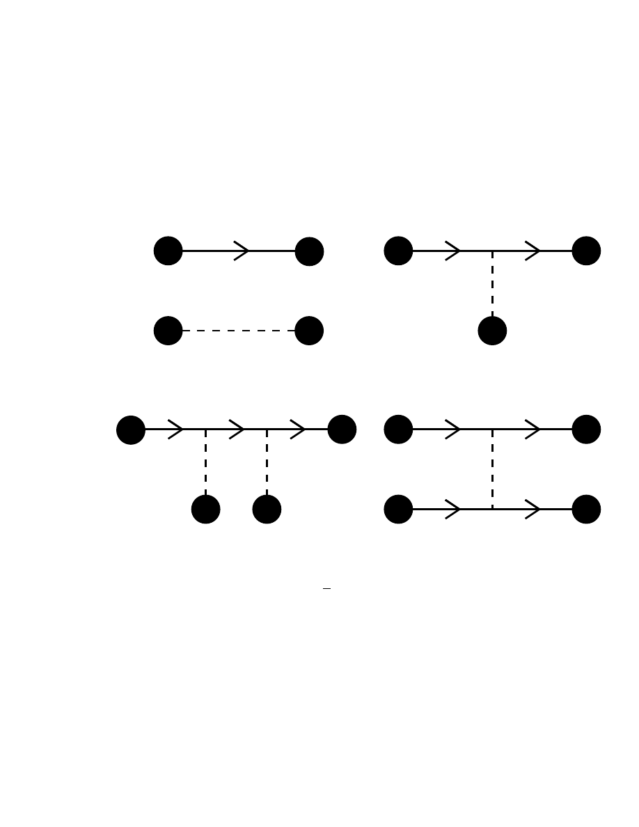
(a)
(c)
(d)
(b)
Figure 1: Tree contributions to iW (η, η, J) with four or fewer sources.
91

×
h
η(x)S(x
− y)S(y − z)η(z)
i
× ∆(y − w)J(w) .
(481)
Our main purpose in this section is to compute the tree-level amplitudes
for various two-body elastic scattering processes, such as e
−
ϕ
→ e
−
ϕ and
e
+
e
−
→ ϕϕ; for these, we will need to evaluate the tree-level contributions to
connected correlation functions of the form
h0|TΨΨϕϕ|0i
C
. Other processes
of interest include e
−
e
−
→ e
−
e
−
and e
+
e
−
→ e
+
e
−
; for these, we will need
to evaluate the tree-level contributions to connected correlation functions of
the form
h0|TΨΨΨΨ|0i
C
.
For
h0|TΨΨϕϕ|0i
C
, the relevant tree-level contribution to iW (η, η, J) is
given by fig. (1)(d). We have
h0|TΨ
α
(x)Ψ
β
(y)ϕ(z
1
)ϕ(z
2
)
|0i
C
=
1
i
δ
δη
α
(x)
i
δ
δη
β
(y)
1
i
δ
δJ(z
1
)
1
i
δ
δJ(z
2
)
iW (η, η, J)
η=η=J=0
=
1
i
5
(ig)
2
Z
d
4
w
1
d
4
w
2
× [S(x−w
1
)S(w
1
−w
2
)S(w
2
−y)]
αβ
× ∆(z
1
−w
1
)∆(z
2
−w
2
)
+
z
1
↔ z
2
+ O(g
4
) .
(482)
The corresponding diagrams, with sources removed, are shown in fig. (2).
For
h0|TΨΨΨΨ|0i
C
, the relevant tree-level contribution to iW (η, η, J) is
given by fig. (1)(c), which has a symmetry factor S = 2. We have
h0|TΨ
α
1
(x
1
)Ψ
β
1
(y
1
)Ψ
α
2
(x
2
)Ψ
β
2
(y
2
)
|0i
C
=
1
i
δ
δη
α
1
(x
1
)
i
δ
δη
β
1
(y
1
)
1
i
δ
δη
α
2
(x
2
)
i
δ
δη
β
2
(y
2
)
iW (η, η, J)
η=η=J=0
.(483)
The two η derivatives can act on the two η’s in the diagram in two different
ways; ditto for the two η derivatives. This results in four different terms,
but two of them are algebraic duplicates of the other two; this duplication
92
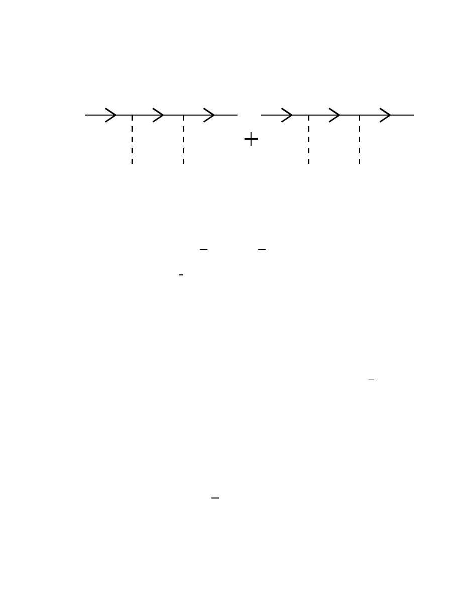
w
w
w
1
1
x
z
1
z
2
y
w
w
w
1
1
x
z
z
y
2
1
Figure 2: Diagrams corresponding to eq. (482).
cancels the symmetry factor (which is a general result). We get
h0|TΨ
α
1
(x
1
)Ψ
β
1
(y
1
)Ψ
α
2
(x
2
)Ψ
β
2
(y
2
)
|0i
C
=
1
i
5
(ig)
2
Z
d
4
w
1
d
4
w
2
× [S(x
1
−w
1
)S(w
1
−y
1
)]
α
1
β
1
× ∆(w
1
−w
2
)
× [S(x
2
−w
2
)S(w
2
−y
2
)]
α
2
β
2
−
(y
1
, β
1
)
↔ (y
2
, β
2
)
+ O(g
4
) .
(484)
The corresponding diagrams, with sources removed, are shown in fig. (3).
Note, however, that we now have a relative minus sign between the two
diagrams, due to the anticommutation of the derivatives with respect to η.
The general rule is this: there is a relative minus sign between any two
diagrams that are identical except for a swap of the position and spin labels
between two external fermion lines.
Let us now consider a particular scattering process: e
−
ϕ
→ e
−
ϕ. The
scattering amplitude is
hf|ii = h0| T a(k
′
)
out
b
s
′
(p
′
)
out
b
†
s
(p)
in
a
†
(k)
in
|0i .
(485)
Next we use the replacements
b
†
s
(p)
in
→ i
Z
d
4
y Ψ(y)(+i
←
/
∂ + m)u
s
(p) e
+ipy
,
(486)
93
x
y
y
x
w
w
2
2
2
1
1
1
x
y
y
x
w
w
2
2
1
1
1
2
Figure 3: Diagrams corresponding to eq. (484).
b
s
′
(p
′
)
out
→ i
Z
d
4
x e
−ipx
u
s
′
(p
′
)(
−i/∂ + m)Ψ(x) ,
(487)
a
†
(k)
in
→ i
Z
d
4
z
1
e
+ikz
1
(
−∂
2
+ m
2
)ϕ(z
1
) ,
(488)
a(k
′
)
out
→ i
Z
d
4
z
2
e
−ik
′
z
2
(
−∂
2
+ m
2
)ϕ(z
2
) .
(489)
We substitute these into eq. (485), and then use eq. (482). The wave oper-
ators (either Klein-Gordon or Dirac) act on the external propagators, and
convert them to delta functions. After using eqs. (478) and (479) for the
internal propagators, all dependence on the various spacetime coordinates is
in the form of plane-wave factors, as in section 10. Integrating over the inter-
nal coordinates then generates delta functions that conserve four-momentum
at each vertex. The only new feature arises from the spinor factors u
s
(p)
and u
s
′
(p
′
). We find that u
s
(p) is associated with the external fermion line
whose arrow points towards the vertex, and that u
s
′
(p
′
) is associated with
the external fermion line whose arrow points away from the vertex. We can
therefore draw the momentum-space diagrams of fig. (4), and write down the
associated tree-level expression for the e
−
ϕ
→ e
−
ϕ scattering amplitude,
i
T
e
−
ϕ→e
−
ϕ
=
1
i
(ig)
2
u
s
′
(p
′
)
"
−/p − /k + m
−s + m
2
+
−/p + /k
′
+ m
−u + m
2
#
u
s
(p) ,
(490)
where s =
−(p + k)
2
and u =
−(p −k
′
)
2
. (We can safely ignore the iǫ’s in the
propagators, because their denominators cannot vanish for any physically
94
p k
k
k
p+k
p
p
k
k
p
p
Figure 4: Diagrams for e
−
ϕ
→ e
−
ϕ, corresponding to eq. (490).
allowed values of s and u.) We will see how to turn this into a more useful
expression in section 46.
Next consider the process e
+
ϕ
→ e
+
ϕ. We now have
hf|ii = h0| T a(k
′
)
out
d
s
′
(p
′
)
out
d
†
s
(p)
in
a
†
(k)
in
|0i .
(491)
The relevant replacements are
d
†
s
(p)
in
→ −i
Z
d
4
x e
+ipx
v
s
(p)(
−i/∂ + m)Ψ(x) ,
(492)
d
s
′
(p
′
)
out
→ −i
Z
d
4
y
Ψ(y)(+i
←
/
∂ + m)v
s
′
(p
′
) e
−ipy
,
(493)
a
†
(k)
in
→ i
Z
d
4
z
1
e
+ikz
1
(
−∂
2
+ m
2
)ϕ(z
1
) ,
(494)
a(k
′
)
out
→ i
Z
d
4
z
2
e
−ikz
2
(
−∂
2
+ m
2
)ϕ(z
2
) .
(495)
We substitute these into eq. (491), and then use eq. (482). This ultimately
leads to the momentum-space Feynman diagrams of fig. (5). Note that we
must now label the external fermion lines with minus their four-momenta;
this is characteristic of d-type particles. (The same phenomenon occurs for a
complex scalar field; see problem 10.1.) Regarding the spinor factors, we find
that
−v
s
(p) is associated with the external fermion line whose arrow points
away
from the vertex, and
−v
s
′
(p
′
) with the external fermion line whose
arrow points towards the vertex. The minus signs attached to each v and
v can be consistently dropped, however, as they only affect the overall sign
95
p k
k
k
p+k
p
p
k
k
p
p
Figure 5: Diagrams for e
+
ϕ
→ e
+
ϕ, corresponding to eq. (496).
of the amplitude (and not the relative signs among contributing diagrams).
The tree-level expression for the e
+
ϕ
→ e
+
ϕ amplitude is then
i
T
e
+
ϕ→e
+
ϕ
=
1
i
(ig)
2
v
s
(p)
"
/
p
− /k
′
+ m
−u + m
2
+
/
p + /
k + m
−s + m
2
#
v
s
′
(p
′
) ,
(496)
where again s =
−(p + k)
2
and u =
−(p − k
′
)
2
.
After working out a few more of these (you might try your hand at some
of them before reading ahead), we can abstract the following set of Feynman
rules.
1) For each incoming electron, draw a solid line with an arrow pointed
towards
the vertex, and label it with the electron’s four-momentum, p
i
.
2) For each outgoing electron, draw a solid line with an arrow pointed
away
from the vertex, and label it with the electron’s four-momentum, p
′
i
.
3) For each incoming positron, draw a solid line with an arrow pointed
away
from the vertex, and label it with minus the positron’s four-momentum,
−p
i
.
4) For each outgoing positron, draw a solid line with an arrow pointed
towards
the vertex, and label it with minus the positron’s four-momentum,
−p
′
i
.
5) For each incoming scalar, draw a dashed line with an arrow pointed
towards
the vertex, and label it with the scalar’s four-momentum, k
i
.
6) For each outgoing scalar, draw a dashed line with an arrow pointed
away
from the vertex, and label it with the scalar’s four-momentum, k
′
i
.
96

7) The only allowed vertex joins two solid lines, one with an arrow point-
ing towards it and one with an arrow pointing away from it, and one dashed
line (whose arrow can point in either direction). Using this vertex, join up
all the external lines, including extra internal lines as needed. In this way,
draw all possible diagrams that are topologically inequivalent.
8) Assign each internal line its own four-momentum. Think of the four-
momenta as flowing along the arrows, and conserve four-momentum at each
vertex. For a tree diagram, this fixes the momenta on all the internal lines.
9) The value of a diagram consists of the following factors:
for each incoming or outgoing scalar, 1;
for each incoming electron, u
s
i
(p
i
);
for each outgoing electron, u
s
′
i
(p
′
i
);
for each incoming positron, v
s
i
(p
i
);
for each outgoing positron, v
s
′
i
(p
′
i
);
for each vertex, ig;
for each internal scalar line,
−i/(k
2
+ M
2
− iǫ),
where k is the four-momentum of that line;
for each internal fermion line,
−i(−/p + m)/(p
2
+ m
2
− iǫ),
where p is the four-momentum of that line.
10) Spinor indices are contracted by starting at one end of a fermion line:
specifically, the end that has the arrow pointing away from the vertex. The
factor associated with the external line is either u or v. Go along the complete
fermion line, following the arrows backwards, and write down (in order from
left to right) the factors associated with the vertices and propagators that
you encounter. The last factor is either a u or v. Repeat this procedure for
the other fermion lines, if any.
11) Two diagrams that are identical except for the momentum and spin
labels on two external fermion lines
that have their arrows pointing in the
same direction
(either both towards or both away from the vertex) have a
relative minus sign.
12) The value of i
T (at tree level) is given by a sum over the values of
the contributing diagrams.
There are additional rules for counterterms and loops, but we will post-
pone those to section 51.
97
1
p
2
k
2
k
1
1
p
p
1
k
1
p
2
k
2
k
1
1
p
p
1
k
1
p
2
k
k
1
p
p
1
k
2
2
Figure 6: Diagrams for e
+
e
−
→ ϕϕ, corresponding to eq. (497).
Let us apply these rules to e
+
e
−
→ ϕϕ. Let the initial electron and
positron have four-momenta p
1
and p
2
, respectively, and the two final scalars
have four-momenta k
′
1
and k
′
2
. The relevant diagrams are shown in fig. (6),
and the result is
i
T
e
+
e
−
→ϕϕ
=
1
i
(ig)
2
v
s
s
(p
2
)
"
−/p
1
+ /
k
′
1
+ m
−t + m
2
+
−/p
1
+ /
k
′
2
+ m
−u + m
2
#
u
s
1
(p
1
) , (497)
where t =
−(p
1
− k
′
1
)
2
and u =
−(p
1
− k
′
2
)
2
.
Next, consider e
−
e
−
→ e
−
e
−
. Let the initial electrons have four-momenta
p
1
and p
2
, and the final electrons have four-momenta p
′
1
and p
′
2
. The relevant
diagrams are shown in fig. (7). It is clear that they are identical except for
the labels on the two external fermion lines that have arrows pointing away
from their vertices. Thus, according to rule #11, these diagrams have a
relative minus sign. (Which diagram gets the extra minus sign is a matter
of convention, and is physically irrelevant.) Thus the result is
i
T
e
−
e
−
→e
−
e
−
=
1
i
(ig)
2
"
(u
′
1
u
1
)(u
′
2
u
2
)
−t + M
2
−
(u
′
2
u
1
)(u
′
1
u
2
)
−u + M
2
#
,
(498)
where u
1
is short for u
s
1
(p
1
), etc., and t =
−(p
1
− p
′
1
)
2
, u =
−(p
1
− p
′
2
)
2
.
One more: e
+
e
−
→ e
+
e
−
. Let the initial electron and positron have four-
momenta p
1
and p
2
, respectively, and the final electron and positron have
four-momenta p
′
1
and p
′
2
, respectively. The relevant diagrams are shown in
fig. (8). If we redraw them in the topologically equivalent manner shown in
98
2
p
1
p
1
p
1
p
1
p
1
p
p
2
2
p
p
2
p
p
1
1
2
p
Figure 7: Diagrams for e
−
e
−
→ e
−
e
−
, corresponding to eq. (498).
fig. (9), then it becomes clear that they are identical except for the labels
on the two external fermion lines that have arrows pointing away from their
vertices. Thus, according to rule #11, these diagrams have a relative minus
sign. (Which diagram gets the extra minus sign is a matter of convention,
and is physically irrelevant.) Thus the result is
i
T
e
+
e
−
→e
+
e
−
=
1
i
(ig)
2
"
(u
′
1
u
1
)(v
2
v
′
2
)
−t + M
2
−
(v
2
u
1
)(u
′
1
v
′
2
)
−u + M
2
#
,
(499)
where s =
−(p
1
+ p
2
)
2
and t =
−(p
1
− p
′
1
)
2
.
Problems
45.1a) Determine how ϕ(x) must transform under parity, time reversal,
and charge conjugation in order for these to all be symmetries of the theory.
(Prerequisite: 39)
b) Same question, but with the interaction given by
L
1
= igϕΨγ
5
Ψ in-
stead of eq. (474).
45.2) Use the Feynman rules to write down (at tree level) i
T for the
processes e
+
e
+
→ e
+
e
+
and ϕϕ
→ e
+
e
−
.
99
p
1
p
1
p
1
p
2
p
2
p
1
p
1
p
2
p
1
p
2
p
1
p
2
+
Figure 8: Diagrams for e
+
e
−
→ e
+
e
−
, corresponding to eq. (499).
p
2
p
1
p
1
p
1
p
2
p
2
p
2
p
1
p
1
p
1
p
2
p
1
Figure 9: Same as fig. (8), but with the diagrams redrawn to show more
clearly that, according to rule #11, they have a relative minus sign.
100

Quantum Field Theory
Mark Srednicki
46: Spin Sums
Prerequisite: 45
In the last section, we calculated various tree-level scattering amplitudes
in Yukawa theory. For example, for e
−
ϕ
→ e
−
ϕ we found
T = g
2
u
s
′
(p
′
)
"
−/p − /k + m
−s + m
2
+
−/p + /k
′
+ m
−u + m
2
#
u
s
(p) ,
(500)
where s =
−(p+k)
2
and u =
−(p−k
′
)
2
. In order to compute the correspond-
ing cross section, we must evaluate
|T |
2
=
T T
∗
. We begin by simplifying
eq. (500) a little; we use (/
p+m)u
s
(p) = 0 to replace the
−/p in each numerator
with m. We then abbreviate eq. (500) as
T = u
′
Au ,
(501)
where
A
≡ g
2
"
−/k + 2m
m
2
− s
+
/
k
′
+ 2m
m
2
− u
#
.
(502)
Then we have
T
∗
=
T = u
′
Au = uAu
′
,
(503)
where in general A
≡ βA
†
β, and, for the particular A of eq. (502), A = A.
Thus we have
|T |
2
= (u
′
Au)(uAu
′
)
=
X
αβγδ
u
′
α
A
αβ
u
β
u
γ
A
γδ
u
′
δ
=
X
αβγδ
u
′
δ
u
′
α
A
αβ
u
β
u
γ
A
γδ
= Tr
h
(u
′
u
′
)A(uu)A
i
.
(504)
101

Next, we use a result from section 38:
u
s
(p)u
s
(p) =
1
2
(1
−sγ
5
/z)(
−/p + m) ,
(505)
where s =
± tells us whether the spin is up or down along the spin quanti-
zation axis z. We then have
|T |
2
=
1
4
Tr
h
(1
−s
′
γ
5
/z
′
)(
−/p
′
+ m)A(1
−sγ
5
/z)(
−/p + m)A
i
.
(506)
We now simply need to take traces of products of gamma matrices; we will
work out the technology for this in the next section.
However, in practice, we are often not interested in (or are unable to easily
measure or prepare) the spin states of the scattering particles. Thus, if we
know that an electron with momentum p
′
landed in our detector, but know
nothing about its spin, we should sum
|T |
2
over the two possible spin states
of this outgoing electron. Similarly, if the spin state of the initial electron is
not specially prepared for each scattering event, then we should average
|T |
2
over the two possible spin states of this initial electron. Then we can use
X
s=±
u
s
(p)u
s
(p) =
−/p + m
(507)
in place of eq. (505).
Let us, then, take
|T |
2
, sum over all final spins, and average over all initial
spins, and call the result
h|T |
2
i. In the present case, we have
h|T |
2
i ≡
1
2
X
s,s
′
|T |
2
=
1
2
Tr
h
(
−/p
′
+ m)A(
−/p + m)A
i
,
(508)
which is much less cumbersome than eq. (506).
Next let’s try something a little harder, namely e
+
e
−
→ e
+
e
−
. We found
in section 45 that
T = g
2
"
(u
′
1
u
1
)(v
2
v
′
2
)
M
2
− t
−
(v
2
u
1
)(u
′
1
v
′
2
)
M
2
− s
#
.
(509)
We then have
T = g
2
"
(u
1
u
′
1
)(v
′
2
v
2
)
M
2
− t
−
(u
1
v
2
)(v
′
2
u
′
1
)
M
2
− s
#
.
(510)
102

When we multiply
T by T , we will get four terms. We want to arrange the
factors in each of them so that every u and every v stands just to the left of
the corresponding u and v. In this way, we get
|T |
2
= +
g
4
(M
2
−t)
2
Tr
h
u
1
u
1
u
′
1
u
′
1
i
Tr
h
v
′
2
v
′
2
v
2
v
2
i
+
g
4
(M
2
−s)
2
Tr
h
u
1
u
1
v
2
v
2
i
Tr
h
v
′
2
v
′
2
u
′
1
u
′
1
i
−
g
4
(M
2
−t)(M
2
−s)
Tr
h
u
1
u
1
v
2
v
2
v
′
2
v
′
2
u
′
1
u
′
1
i
−
g
4
(M
2
−s)(M
2
−t)
Tr
h
u
1
u
1
u
′
1
u
′
1
v
′
2
v
′
2
v
2
v
2
i
.
(511)
Then we average over initial spins and sum over final spins, and use eq. (507)
and
X
s=±
v
s
(p)v
s
(p) =
−/p − m .
(512)
We then must evaluate traces of products of up to four gamma matrices.
103

Quantum Field Theory
Mark Srednicki
47: Gamma Matrix Technology
Prerequisite: 36
In this section, we will learn some tricks for handling gamma matrices.
We need the following information as a starting point:
{γ
µ
, γ
ν
} = −2g
µν
,
(513)
γ
2
5
= 1 ,
(514)
{γ
µ
, γ
5
} = 0 ,
(515)
Tr 1 = 4 .
(516)
Now consider the trace of the product of n gamma matrices. We have
Tr[γ
µ
1
. . . γ
µ
n
] = Tr[γ
2
5
γ
µ
1
γ
2
5
. . . γ
2
5
γ
µ
n
]
= Tr[(γ
5
γ
µ
1
γ
5
) . . . (γ
5
γ
µ
n
γ
5
)]
= Tr[(
−γ
2
5
γ
µ
1
) . . . (
−γ
2
5
γ
µ
n
)]
= (
−1)
n
Tr[γ
µ
1
. . . γ
µ
n
] .
(517)
We used eq. (514) to get the first equality, the cyclic property of the trace
for the second, eq. (515) for the third, and eq. (514) again for the fourth. If
n is odd, eq. (517) tells us that this trace is equal to minus itself, and must
therefore be zero:
Tr[ odd # of γ
µ
’s ] = 0 .
(518)
Similarly,
Tr[ γ
5
( odd # of γ
µ
’s ) ] = 0 .
(519)
104

Next, consider Tr[γ
µ
γ
ν
]. We have
Tr[γ
µ
γ
ν
] = Tr[γ
ν
γ
µ
]
=
1
2
Tr[γ
µ
γ
ν
+ γ
ν
γ
µ
]
=
−g
µν
Tr 1
=
−4g
µν
.
(520)
The first equality follows from the cyclic property of the trace, the second
averages the left- and right-hand sides of the first, the third uses eq. (513),
and the fourth uses eq. (516).
A slightly nicer way of expressing eq. (520) is to introduce two arbitrary
four-vectors a
µ
and b
µ
, and write
Tr[/a/b] =
−4(ab) ,
(521)
where /a = a
µ
γ
µ
, /b = b
µ
γ
µ
, and (ab) = a
µ
b
µ
.
Next consider Tr[/a/b/c/d]. We evaluate this by moving /a to the right, using
eq. (513), which is now more usefully written as
/a/b =
−/b/a − 2(ab) .
(522)
Using this repeatedly, we have
Tr[/a/b/c/d] =
−Tr[/b/a/c/d] − 2(ab)Tr[/c/d]
= +Tr[/b/c/a/d] + 2(ac)Tr[/b/d]
− 2(ab)Tr[/c/d]
=
−Tr[/b/c/d/a] − 2(ad)Tr[/b/c] + 2(ac)Tr[/b/d] − 2(ab)Tr[/c/d] .
(523)
Now we note that the first term on the right-hand side of the last line is, by
the cyclic property of the trace, actually equal to minus the left-hand side.
We can then move this term to the left-hand side to get
2 Tr[/a/b/c/d] =
− 2(ad)Tr[/b/c] + 2(ac)Tr[/b/d] − 2(ab)Tr[/c/d] .
(524)
Finally, we evaluate each Tr[/a/b] with eq. (521), and divide by two:
Tr[/a/b/c/d] = 4
h
(ad)(bc)
− (ac)(bd) + (ab)(cd)
i
.
(525)
105

This is our final result for this trace.
Clearly, we can use the same technique to evaluate the trace of the product
of any even number of gamma matrices.
Next, let’s consider traces that involve γ
5
’s and γ
µ
’s. Since
{γ
5
, γ
µ
} = 0,
we can always bring all the γ
5
’s together by moving them through the γ
µ
’s
(generating minus signs as we go). Then, since γ
2
5
= 1, we end up with either
one γ
5
or none. So we need only consider Tr[γ
5
γ
µ
1
. . . γ
µ
n
]. And, according
to eq. (519), we need only be concerned with even n.
Recall that an explicit formula for γ
5
is
γ
5
= iγ
0
γ
1
γ
2
γ
3
.
(526)
Eq. (525) then implies
Tr γ
5
= 0 .
(527)
Similarly, the six-matrix generalization of eq. (525) yields
Tr[γ
5
γ
µ
γ
ν
] = 0 .
(528)
Finally, consider Tr[γ
5
γ
µ
γ
ν
γ
ρ
γ
σ
]. The only way to get a nonzero result is to
have the four vector indices take on four different values. If we consider the
special case Tr[γ
5
γ
3
γ
2
γ
1
γ
0
], plug in eq. (526), and then use (γ
i
)
2
=
−1 and
(γ
0
)
2
= 1, we get i(
−1)
3
Tr 1 =
−4i, or equivalently
Tr[γ
5
γ
µ
γ
ν
γ
ρ
γ
σ
] =
−4iε
µνρσ
,
(529)
where ε
0123
= ε
3210
= +1.
Another category of gamma matrix combinations that we will eventually
encounter is γ
µ
/a . . . γ
µ
. The simplest of these is
γ
µ
γ
µ
= g
µν
γ
µ
γ
ν
=
1
2
g
µν
{γ
µ
, γ
ν
}
=
−g
µν
g
µν
=
−d .
(530)
To get the second equality, we used the fact that g
µν
is symmetric, and
so only the symmetric part of γ
µ
γ
ν
contributes. In the last line, d is the
106

number of spacetime dimensions. Of course, our entire spinor formalism has
been built around d = 4, but we will need formal results for d = 4
−ε when
we dimensionally regulate loop diagrams involving fermions.
We move on to evaluate
γ
µ
/aγ
µ
= γ
µ
(
−γ
µ
/a
− 2a
µ
)
=
−γ
µ
γ
µ
/a
− 2/a
= (d
−2)/a .
(531)
We continue with
γ
µ
/a/bγ
µ
= (
−/aγ
µ
− 2a
µ
)(
−γ
µ
/b
− 2b
µ
)
= /aγ
µ
γ
µ
/b + 2/a/b + 2/a/b + 4(ab)
= 4(ab)
− (d−4)/a/b .
(532)
And finally,
γ
µ
/a/b/cγ
µ
= (
−/aγ
µ
− 2a
µ
)/b(
−γ
µ
/c
− 2c
µ
)
= /aγ
µ
/bγ
µ
/c + 2/b/a/c + 2/a/c/b + 4(ac)/b
= (d
−2)/a/b/c + 2/b/a/c + 2[/a/c + 2(ac)]/b
= (d
−2)/a/b/c + 2/b/a/c − 2/c/a/b
= (d
−2)/a/b/c + 2[−/a/b − 2(ab)]/c − 2/c/a/b
= (d
−4)/a/b/c − 4(ab)/c − 2/c/a/b
= (d
−4)/a/b/c + 2/c[−2(ab) − /a/b]
= 2/c/b/a + (d
−4)/a/b/c .
(533)
107

Quantum Field Theory
Mark Srednicki
48: Spin-Averaged Cross Sections in Yukawa Theory
Prerequisite: 46, 47
In section 46, we computed
|T |
2
for (among other processes) e
+
e
−
→
e
+
e
−
. We take the incoming and outgoing electrons to have momenta p
1
and
p
′
1
, respectively, and the incoming and outgoing positrons to have momenta
p
2
and p
′
2
, respectively. We have p
2
i
= p
′2
i
=
−m
2
, where m is the electron
(and positron) mass. The Mandelstam variables are
s =
−(p
1
+ p
2
)
2
=
−(p
′
1
+ p
′
2
)
2
,
t =
−(p
1
− p
′
1
)
2
=
−(p
2
− p
′
2
)
2
,
u =
−(p
1
− p
′
2
)
2
=
−(p
2
− p
′
1
)
2
,
(534)
and they obey s + t + u = 4m
2
. Our result was
|T |
2
= g
4
"
Φ
ss
(M
2
− s)
2
−
Φ
st
+ Φ
ts
(M
2
− s)(M
2
− t)
+
Φ
tt
(M
2
− t)
2
#
,
(535)
where M is the scalar mass, and
Φ
ss
= Tr
h
u
1
u
1
v
2
v
2
i
Tr
h
v
′
2
v
′
2
u
′
1
u
′
1
i
,
Φ
tt
= Tr
h
u
1
u
1
u
′
1
u
′
1
i
Tr
h
v
′
2
v
′
2
v
2
v
2
i
,
Φ
st
= Tr
h
u
1
u
1
u
′
1
u
′
1
v
′
2
v
′
2
v
2
v
2
i
,
Φ
ts
= Tr
h
u
1
u
1
v
2
v
2
v
′
2
v
′
2
u
′
1
u
′
1
i
.
(536)
Next, we average over the two initial spins and sum over the two final
spins to get
h|T |
2
i =
1
4
X
s
1
,s
2
,s
′
1
,s
′
2
|T |
2
.
(537)
108

Then we use
X
s=±
u
s
(p)u
s
(p) =
−/p + m ,
X
s=±
v
s
(p)v
s
(p) =
−/p − m ,
(538)
to get
hΦ
ss
i =
1
4
Tr
h
(
−/p
1
+m)(
−/p
2
−m)
i
Tr
h
(
−/p
′
2
−m)(−/p
′
1
+m)
i
,
(539)
hΦ
tt
i =
1
4
Tr
h
(
−/p
1
+m)(
−/p
′
1
+m)
i
Tr
h
(
−/p
′
2
−m)(−/p
2
−m)
i
,
(540)
hΦ
st
i =
1
4
Tr
h
(
−/p
1
+m)(
−/p
′
1
+m)(
−/p
′
2
−m)(−/p
2
−m)
i
,
(541)
hΦ
ts
i =
1
4
Tr
h
(
−/p
1
+m)(
−/p
2
−m)(−/p
′
2
−m)(−/p
′
1
+m)
i
.
(542)
It is now merely tedious to evaluate these traces with the technology of
section 47.
For example,
Tr
h
(
−/p
1
+m)(
−/p
2
−m)
i
= Tr[/
p
1
/
p
2
]
− m
2
Tr 1
=
−4(p
1
p
2
)
− 4m
2
,
(543)
It is convenient to write four-vector products in terms of the Mandelstam
variables. We have
p
1
p
2
= p
′
1
p
′
2
=
−
1
2
(s
− 2m
2
) ,
p
1
p
′
1
= p
2
p
′
2
= +
1
2
(t
− 2m
2
) ,
p
1
p
′
2
= p
′
1
p
2
= +
1
2
(u
− 2m
2
) ,
(544)
and so
Tr
h
(
−/p
1
+m)(
−/p
2
−m)
i
= 2s
− 8m
2
.
(545)
Thus, we can easily work out eqs. (539) and (540):
hΦ
ss
i = (s − 4m
2
)
2
,
(546)
hΦ
tt
i = (t − 4m
2
)
2
.
(547)
109

Obviously, if we start with
hΦ
ss
i and make the swap s ↔ t, we get hΦ
tt
i.
We could have anticipated this from eqs. (539) and (540): if we start with
the right-hand side of eq. (539) and make the swap p
2
↔ −p
′
1
, we get the
right-hand side of eq. (540). But from eq. (544), we see that this momentum
swap is equivalent to s
↔ t.
Let’s move on to
hΦ
st
i and hΦ
ts
i. These two are also related by p
2
↔ −p
′
1
,
and so we only need to compute one of them. We have
hΦ
st
i =
1
4
Tr[/
p
1
/
p
′
1
/
p
′
2
/
p
2
] +
1
4
m
2
Tr[/
p
1
/
p
′
1
− /p
1
/
p
′
2
− /p
1
/
p
2
− /p
′
1
/
p
′
2
− /p
′
1
/
p
2
+ /
p
′
2
/
p
2
]
+
1
4
m
4
Tr 1
= (p
1
p
′
1
)(p
2
p
′
2
)
− (p
1
p
′
2
)(p
2
p
′
1
) + (p
1
p
2
)(p
′
1
p
′
2
)
− m
2
[p
1
p
′
1
− p
1
p
′
2
− p
1
p
2
− p
′
1
p
′
2
+ p
′
1
p
2
+ p
2
p
′
2
] + m
4
=
−
1
2
st + 2m
2
u .
(548)
To get the last line, we used eq. (544), and then simplified it as much as
possible via s + t + u = 4m
2
. Since our result is symmetric on s
↔ t, we have
hΦ
ts
i = hΦ
st
i.
Putting all of this together, we get
h|T |
2
i = g
4
"
(s
− 4m
2
)
2
(M
2
− s)
2
+
st
− 4m
2
u
(M
2
− s)(M
2
− t)
+
(t
− 4m
2
)
2
(M
2
− t)
2
#
.
(549)
This can then be converted to a differential cross section (in any frame) via
the formulae of section 11.
Let’s do one more: e
−
ϕ
→ e
−
ϕ. We take the incoming and outgoing
electrons to have momenta p and p
′
, respectively, and the incoming and
outgoing scalars to have momenta k and k
′
, respectively. We then have
p
2
= p
′2
=
−m
2
and k
2
= k
′2
=
−M
2
. The Mandelstam variables are
s =
−(p + k)
2
=
−(p
′
+ k
′
)
2
,
t =
−(p − p
′
)
2
=
−(k − k
′
)
2
,
u =
−(p − k
′
)
2
=
−(k − p
′
)
2
,
(550)
and they obey s + t + u = 2m
2
+ 2M
2
. Our result in section 46 was
h|T |
2
i =
1
2
Tr
h
A(
−/p + m)A(−/p
′
+ m)
i
,
(551)
110

where
A = g
2
"
−/k + 2m
m
2
− s
+
/
k
′
+ 2m
m
2
− u
#
.
(552)
Thus we have
h|T |
2
i = g
4
"
hΦ
ss
i
(m
2
− s)
2
+
hΦ
su
i + hΦ
us
i
(m
2
− s)(m
2
− u)
+
hΦ
uu
i
(m
2
− u)
2
#
,
(553)
where now
hΦ
ss
i =
1
2
Tr
h
(
−/p
′
+m)(
−/k+2m)(−/p+m)(−/k+2m)
i
,
(554)
hΦ
uu
i =
1
2
Tr
h
(
−/p
′
+m)(+/
k
′
+2m)(
−/p+m)(+/k
′
+2m)
i
,
(555)
hΦ
su
i =
1
2
Tr
h
(
−/p
′
+m)(
−/k+2m)(−/p+m)(+/k
′
+2m)
i
,
(556)
hΦ
us
i =
1
2
Tr
h
(
−/p
′
+m)(+/
k
′
+2m)(
−/p+m)(−/k+2m)
i
.
(557)
We can evaluate these in terms of the Mandelstam variables by using our
trace technology, along with
pk = p
′
k
′
=
−
1
2
(s
− m
2
− M
2
) ,
pp
′
= +
1
2
(t
− 2m
2
) ,
kk
′
= +
1
2
(t
− 2M
2
) ,
pk
′
= p
′
k = +
1
2
(u
− m
2
− M
2
) .
(558)
Examining eqs. (554) and (555), we see that
hΦ
ss
i and hΦ
uu
i are transformed
into each other by k
↔ −k
′
. Examining eqs. (556) and (557), we see that
hΦ
su
i and hΦ
us
i are also transformed into each other by k ↔ −k
′
. From
eq. (558), we see that this is equivalent to s
↔ u. Thus we need only compute
hΦ
ss
i and hΦ
su
i, and then take s ↔ u to get hΦ
uu
i and hΦ
us
i. This is, again,
merely tedious, and the results are
hΦ
ss
i = −su + m
2
(9s + u) + 7m
4
− 8m
2
M
2
+ M
4
,
(559)
hΦ
uu
i = −su + m
2
(9u + s) + 7m
4
− 8m
2
M
2
+ M
4
,
(560)
hΦ
su
i = +su + 3m
2
(s + u) + 9m
4
− 8m
2
M
2
− M
4
.
(561)
hΦ
us
i = +su + 3m
2
(s + u) + 9m
4
− 8m
2
M
2
− M
4
.
(562)
111

Problems
48.1) The tedium of these calculations is greatly alleviated by making use
of a symbolic manipulation program like Mathematica or Maple. One ap-
proach is brute force: compute 4
×4 matrices like /p in the CM frame, and take
their products and traces. If you are familiar with a symbolic-manipulation
program, write one that does this. See if you can verify eqs. (559–562).
48.2) Compute
h|T |
2
i for e
−
e
−
→ e
−
e
−
. You should find that your result
is the same as that for e
+
e
−
→ e
+
e
−
, but with s
↔ u, and an extra overall
minus sign. This relationship is known as crossing symmetry.
48.3) Compute
h|T |
2
i for e
+
e
−
→ ϕϕ. You should find that your result
is the same as that for e
−
ϕ
→ e
−
ϕ, but with s
↔ t, and an extra overall
minus sign. This is another example of crossing symmetry.
48.4) Suppose that M > 2m, so that the scalar can decay to an electron-
positron pair.
a) Compute the decay rate, summed over final spins.
b) Compute
|T |
2
for decay into an electron with spin s
1
and a positron
with spin s
2
. Take the fermion three-momenta to be along the z axis, and
let the x-axis be the spin-quantization axis. You should find that
|T |
2
= 0
if s
1
=
−s
2
, or if M = 2m (so that the outgoing three-momentum of each
fermion is zero). Discuss this in light of conservation of angular momentum
and of parity. (Prerequisite: 40.)
c) Compute the rate for decay into an electron with helicity s
1
and a
positron with helicity s
2
. (See section 38 for the definition of helicity.) You
should find that the decay rate is zero if s
1
=
−s
2
. Discuss this in light of
conservation of angular momentum and of parity.
d) Now consider changing the interaction to
L
1
= igϕΨγ
5
Ψ, and compute
the spin-summed decay rate. Explain (in light of conservation of angular
momentum and of parity) why the decay rate is larger than it was without
the iγ
5
in the interaction.
e) Repeat parts (b) and (c) for the new form of the interaction, and
explain any differences in the results.
48.5) The charged pion π
−
is represented by a complex scalar field ϕ, the
muon
µ
−
by a Dirac field
M, and the muon neutrino ν
µ
by a spin-projected
112

Dirac field P
L
N , where P
L
=
1
2
(1
−γ
5
). The charged pion can decay to a
muon and a muon antineutrino via the interaction
L
1
= 2c
1
G
F
f
π
∂
µ
ϕ
Mγ
µ
P
L
N + h.c. ,
(563)
where c
1
is the cosine of the Cabibbo angle, G
F
= is the Fermi constant, and
f
π
is the pion decay constant.
a) Compute the charged pion decay rate Γ (at tree level).
b) The charged pion mass is m
π
= 139.6 MeV, the muon mass is m
µ
=
105.7 MeV, and the muon neutrino is massless. The Fermi constant is mea-
sured in muon decay to be G
F
= 1.166
× 10
−5
GeV
−2
, and the cosine of the
the Cabibbo angle is measured in nuclear beta decays to be c
1
= 0.974. The
measured value of the charged pion lifetime is 2.603
× 10
−8
s. Determine the
value of f
π
in MeV.
113

Quantum Field Theory
Mark Srednicki
49: The Feynman Rules for Majorana Fields
Prerequisite: 45
In this section we will deduce the Feynman rules for Yukawa theory, but
with a Majorana field instead of a Dirac field. We can think of the particles
associated with the Majorana field as massive neutrinos.
We have
L
1
=
1
2
gϕΨΨ
=
1
2
gϕΨ
T
CΨ ,
(564)
where Ψ be a Majorana field (with mass m) and ϕ is a real scalar field (with
mass M), and g is a coupling constant. In this section, we will be concerned
with tree-level processes only, and so we omit renormalizing Z factors.
From section 41, we have the LSZ rules appropriate for a Majorana field,
b
†
s
(p)
in
→ −i
Z
d
4
x e
+ipx
v
s
(p)(
−i/∂ + m)Ψ(x)
(565)
= +i
Z
d
4
x Ψ
T
(x)
C(+i
←
/
∂ + m)u
s
(p)e
+ipx
,
(566)
b
s
′
(p
′
)
out
→ +i
Z
d
4
x e
−ip
′
x
u
s
′
(p
′
)(
−i/∂ + m)Ψ(x) ,
(567)
=
−i
Z
d
4
x e
−ip
′
x
Ψ
T
(x)
C(+i
←
/
∂ + m)v
s
′
(p
′
)e
−ip
′
x
. (568)
Eq. (566) follows from eq. (565) by taking the transpose of the right-hand
side, and using v
s
′
(p
′
)
T
=
−Cu
s
′
(p
′
) and (
−i/∂ + m)
T
=
C(+i/∂ + m)C
−1
;
similarly, eq. (568) follows from eq. (567). Which form we use depends on
convenience, and is best chosen on a diagram-by-diagram basis, as we will
see shortly.
114

Eqs. (565–568) lead us to compute correlation functions containing Ψ’s,
but not Ψ’s. In position space, this leads to Feynman rules where the fermion
propagator is
1
i
S(x
− y)C
−1
, and the ϕΨΨ vertex is ig
C; the factor of
1
2
in
L
1
is killed by a symmetry factor of 2! that arises from having two identical
Ψ fields in
L
1
. In a particular diagram, as we move along a fermion line, the
C
−1
in the propagator will cancel against the
C in the vertex, leaving over a
final
C
−1
at one end. This
C
−1
can be canceled by a
C from eq. (566) (for an
incoming particle) or (568) (for an outgoing particle). On the other hand, for
the other end of the same line, we should use either eq. (565) (for an incoming
particle) or eq. (567) (for an outgoing particle) to avoid introducing an extra
C at that end. In this way, we can avoid ever having explicit factors of C in
our Feynman rules.
Using this approach, the Feynman rules for this theory are as follows.
1) The total number of incoming and outgoing neutrinos is always even;
call this number 2n. Draw n solid lines. Connect them with internal dashed
lines, using a vertex that joins one dashed and two solid lines. Also, attach
an external dashed line for each incoming or outgoing scalar. In this way,
draw all possible diagrams that are topologically inequivalent.
2) Draw arrows on each segment of each solid line; keep the arrow direc-
tion continuous along each line.
3) Label each external dashed line with the momentum of an incoming
or outgoing scalar. If the particle is incoming, draw an arrow on the dashed
line that points towards the vertex; If the particle is outgoing, draw an arrow
on the dashed line that points away from the vertex.
4) Label each external solid line with the momentum of an incoming or
outgoing neutrino, but include a minus sign with the momentum if (a) the
particle is incoming and the arrow points away from the vertex, or (b) the
particle is outgoing and the arrow points towards the vertex.
5) Do this labeling of external lines in all possible inequivalent ways. Two
diagrams are considered equivalent if they can be transformed into each other
by reversing all the arrows on one or more fermion lines, and correspondingly
changing the signs of the external momenta on each reversed-arrow line. The
process of arrow reversal contributes a minus sign for each reversed-arrow
line.
115

6) Assign each internal line its own four-momentum. Think of the four-
momenta as flowing along the arrows, and conserve four-momentum at each
vertex. For a tree diagram, this fixes the momenta on all the internal lines.
9) The value of a diagram consists of the following factors:
for each incoming or outgoing scalar, 1;
for each incoming neutrino labeled with +p
i
, u
s
i
(p
i
);
for each incoming neutrino labeled with
−p
i
, v
s
i
(p
i
);
for each outgoing neutrino labeled with +p
′
i
, u
s
′
i
(p
′
i
);
for each outgoing neutrino labeled with
−p
′
i
, v
s
′
i
(p
′
i
);
for each vertex, ig;
for each internal scalar line,
−i/(k
2
+ M
2
− iǫ),
where k is the four-momentum of that line;
for each internal fermion line,
−i(−/p + m)/(p
2
+ m
2
− iǫ),
where p is the four-momentum of that line.
10) Spinor indices are contracted by starting at one end of a fermion line:
specifically, the end that has the arrow pointing away from the vertex. The
factor associated with the external line is either u or v. Go along the complete
fermion line, following the arrows backwards, and writing down (in order from
left to right) the factors associated with the vertices and propagators that
you encounter. The last factor is either a u or v. Repeat this procedure for
the other fermion lines, if any.
11) Two diagrams that are identical except for the momentum and spin
labels on two external fermion lines
that have their arrows pointing in the
same direction
(either both towards or both away from the vertex) have a
relative minus sign.
12) The value of i
T is given by a sum over the values of all these diagrams.
There are additional rules for counterterms and loops, but we will post-
pone those to section 51.
Let’s look at the simplest process, ϕ
→ νν. There are two possible
diagrams for this, shown in fig. (10). However, according to rule #5, these
two diagrams are equivalent. The first one evaluates to
i
T = ig v
′
2
u
′
1
,
(569)
116
p
2
p
1
k
p
1
p
2
k
Figure 10: Two equivalent diagrams for ϕ
→ νν, corresponding to eqs. (569)
and (570), respectively.
while the second gives
i
T = −ig v
′
1
u
′
2
.
(570)
The minus sign comes from the last part of rule #5: reversing the arrows on
one fermion line gives an extra minus sign. These two versions of
T should
of course yield the same result; to check this, note that
v
1
u
2
= [v
1
u
2
]
T
= u
T
2
v
T
1
= v
2
C
−1
C
−1
u
1
=
−v
2
u
1
,
(571)
as required.
In general, for processes with a total of just two incoming and outgoing
neutrinos, such as νϕ
→ νϕ or νν → ϕϕ, these rules give (up to an irrelevant
overall sign) the same result for i
T as we would get for the corresponding
process in the Dirac case, e
−
ϕ
→ e
−
ϕ or e
+
e
−
→ ϕϕ. (Note, however, that
in the Dirac case, we have
L
1
= gϕΨΨ, as compared with
L
1
=
1
2
gϕ
ΨΨ in
the Majorana case.)
The differences between Dirac and Majorana fermions become more pro-
nounced for νν
→ νν. Now there are three inequivalent contributing dia-
grams, shown in fig. (11). The corresponding amplitude can be written as
i
T =
1
i
(ig)
2
"
(u
′
1
u
1
)(u
′
2
u
2
)
−t + M
2
−
(u
′
2
u
1
)(u
′
1
u
2
)
−u + M
2
+
(v
2
u
1
)(u
′
1
v
′
2
)
−s + M
2
#
,
(572)
117
2
p
1
p
1
p
1
p
2
p
2
p
1
p
2
p
2
p
1
p
2
p
2
p
1
p
1
p
1
p
2
p
1
p
1
p
Figure 11: Diagrams for νν
→ νν, corresponding to eq. (572).
118

where s =
−(p
1
+ p
2
)
2
, t =
−(p
1
− p
′
1
)
2
and u =
−(p
1
− p
′
2
)
2
. Note the
relative signs. After taking the absolute square of this expression, we can use
relations like eq. (571) on a term-by-term basis to put everything into a form
that allows the spin sums to be performed in the standard way.
In fact, we have already done all the necessary work in the Dirac case.
The s-s, s-t, and t-t terms in
h|T |
2
i for νν → νν are the same as those for
e
+
e
−
→ e
+
e
−
, while the t-t, t-u, and u-u terms are the same as those for
the crossing-related process e
−
e
−
→ e
−
e
−
. Finally, the s-u terms can be
obtained from the s-t terms via t
↔ u, or equivalently from the t-u terms
via t
↔ s. Thus the result is
h|T |
2
i = g
4
"
(s
− 4m
2
)
2
(M
2
− s)
2
+
st
− 4m
2
u
(M
2
− s)(M
2
− t)
+
(t
− 4m
2
)
2
(M
2
− t)
2
+
tu
− 4m
2
s
(M
2
− t)(M
2
− u)
+
(u
− 4m
2
)
2
(M
2
− u)
2
+
us
− 4m
2
t
(M
2
− u)(M
2
− s)
#
,
(573)
which is neatly symmetric on permutations of s, t, and u.
119

Quantum Field Theory
Mark Srednicki
50: Massless Particles and Spinor Helicity
Prerequisite: 48
Scattering amplitudes often simplify greatly if the particles are massless
(or can be approximated as massless because the Mandelstam variables all
have magnitudes much larger than the particle masses squared). In this
section we will explore this phenomenon for spin-one-half (and spin-zero)
particles. We will begin developing the technology of spinor helicity, which
will prove to be of indispensible utility in Part III.
Recall from section 38 that the u spinors for a massless spin-one-half
particle obey
u
s
(p)u
s
(p) =
1
2
(1 + sγ
5
)(
−/p) ,
(574)
where s =
± specifies the helicity, the component of the particle’s spin
measured along the axis specified by its three-momentum; in this notation
the helicity is
1
2
s. The v spinors obey a similar relation,
v
s
(p)v
s
(p) =
1
2
(1
− sγ
5
)(
−/p) .
(575)
In fact, in the massless case, with the phase conventions of section 38, we
have v
s
(p) = u
−s
(p). Thus we can confine our discussion to u-type spinors
only, since we need merely change the sign of s to accomodate v-type spinors.
Let us consider a u spinor for a particle of negative helicity. We have
u
−
(p)u
−
(p) =
1
2
(1
− γ
5
)(
−/p) .
(576)
Let us define
p
a ˙a
≡ p
µ
σ
µ
a ˙a
.
(577)
Then we also have
p
˙aa
= ε
ac
ε
˙a ˙c
p
c ˙c
= p
µ
¯
σ
µ ˙aa
.
(578)
120

Then, using
γ
µ
=
0
σ
µ
¯
σ
µ
0
!
,
1
2
(1
− γ
5
) =
1 0
0 0
!
(579)
in eq. (576), we find
u
−
(p)u
−
(p) =
0
−p
a ˙a
0
0
!
.
(580)
On the other hand, we know that the lower two components of u
−
(p) vanish,
and so we can write
u
−
(p) =
φ
a
0
!
.
(581)
Here φ
a
is a two-component numerical spinor; it is not an anticommuting
object. Such a commuting spinor is sometimes called a twistor. An explicit
numerical formula for it (verified in problem 50.1) is
φ
a
=
√
2ω
− sin(
1
2
θ)e
−iφ
+ cos(
1
2
θ)
!
,
(582)
where θ and φ are the polar and azimuthal angles that specify the direction
of the three-momentum p, and ω =
|p|. Barring eq. (581) yields
u
−
(p) = ( 0, φ
∗
˙a
) ,
(583)
where φ
∗
˙a
= (φ
a
)
∗
. Now, combining eqs. (581) and (583), we get
u
−
(p)u
−
(p) =
0 φ
a
φ
∗
˙a
0
0
!
.
(584)
Comparing with eq. (580), we see that
p
a ˙a
=
−φ
a
φ
∗
˙a
.
(585)
This expresses the four-momentum of the particle neatly in terms of the
twistor that describes its spin state. The essence of the spinor helicity method
is to treat φ
a
as the fundamental object, and to express the particle’s four-
momentum in terms of it, via eq. (585).
121

Given eq. (581), and the phase conventions of section 38, the positive-
helicity spinor is
u
+
(p) =
0
φ
∗ ˙a
!
,
(586)
where φ
∗ ˙a
= ε
˙a ˙c
φ
∗
˙c
. Barring eq. (586) yields
u
+
(p) = ( φ
a
, 0 ) .
(587)
Computation of u
+
(p)u
+
(p) via eqs. (586) and (587), followed by comparison
with eq. (574) with s = +, then reproduces eq. (585), but with the indices
raised.
In fact, the decomposition of p
a ˙a
into the direct product of a twistor and
its complex conjugate is unique (up to an overall phase for the twistor). To
see this, use σ
µ
= (I, ~σ) to write
p
a ˙a
=
−p
0
+ p
3
p
1
− ip
2
p
1
+ ip
2
−p
0
− p
3
!
.
(588)
The determinant of this matrix is
−(p
0
)
2
+ p
2
, and this vanishes because the
particle is (by assumption) massless. Thus p
a ˙a
has a zero eigenvalue. There-
fore, it can be written as a projection onto the eigenvector corresponding to
the nonzero eigenvalue. That is what eq. (585) represents, with the nonzero
eigenvalue absorbed into the normalization of the eigenvector φ
a
.
Let us now introduce some useful notation. Let p and k be two four-
momenta, and φ
a
and κ
a
the corresponding twistors. We define the twistor
product
[p k]
≡ φ
a
κ
a
.
(589)
Because φ
a
κ
a
= ε
ac
φ
c
κ
a
, and the twistors commute, we have
[k p] =
−[p k] .
(590)
From eqs. (581) and (587), we can see that
u
+
(p)u
−
(k) = [p k] .
(591)
Similarly, let us define
hp ki ≡ φ
∗
˙a
κ
∗ ˙a
.
(592)
122

Comparing with eq. (589) we see that
hp ki = [k p]
∗
,
(593)
which implies that this product is also antisymmetric,
hk pi = −hp ki .
(594)
Also, from eqs. (583) and (586), we have
u
−
(p)u
+
(k) =
hp ki .
(595)
Note that the other two possible spinor products vanish:
u
+
(p)u
+
(k) = u
−
(p)u
−
(k) = 0 .
(596)
The twistor products
hp ki and [p k] satisfy another important relation,
hp ki[k p] = (φ
∗
˙a
κ
∗ ˙a
)(κ
a
φ
a
)
= (φ
∗
˙a
φ
a
)(κ
a
κ
∗ ˙a
)
= p
˙aa
k
a ˙a
=
−2p
µ
k
µ
,
(597)
where the last line follows from ¯
σ
µ ˙aa
σ
ν
a ˙a
=
−2g
µν
.
Let us apply this notation to the tree-level scattering amplitude for e
−
ϕ
→
e
−
ϕ in Yukawa theory, which we first computed in Section 44, and which
reads
T
s
′
s
= g
2
u
s
′
(p
′
)
h
˜
S(p+k) + ˜
S(p
−k
′
)
i
u
s
(p) .
(598)
For a massless fermion, ˜
S(p) =
−/p/p
2
. If the scalar is also massless, then
(p + k)
2
= 2p
· k and (p − k
′
)
2
=
−2p · k
′
. Also, we can remove the /
p’s in the
propagator numerators in eq. (598), because /
pu
s
(p) = 0. Thus we have
T
s
′
s
= g
2
u
s
′
(p
′
)
"
−/k
2p
·k
+
−/k
′
2p
·k
′
#
u
s
(p) .
(599)
123

Now consider the case s
′
= s = +. From eqs. (586), (587), and
−/k =
0
κ
a
κ
∗
˙a
κ
∗ ˙a
κ
a
0
!
,
(600)
we get
u
+
(p
′
)(
−/k)u
+
(p) = φ
′a
κ
a
κ
∗
˙a
φ
∗ ˙a
= [p
′
k]
hk pi .
(601)
Similarly, for s
′
= s =
−, we find
u
−
(p
′
)(
−/k)u
−
(p) = φ
′∗
˙a
κ
∗ ˙a
κ
a
φ
a
=
hp
′
k
i [k p] ,
(602)
while for s
′
6= s, the amplitude vanishes:
u
−
(p
′
)(
−/k)u
+
(p) = u
+
(p
′
)(
−/k)u
−
(p) = 0 .
(603)
Then, using eq. (597) on the denominators in eq. (599), we find
T
++
=
−g
2
[p
′
k]
[p k]
+
[p
′
k
′
]
[p k
′
]
!
,
T
−−
=
−g
2
hp
′
k
i
hp ki
+
hp
′
k
′
i
hp k
′
i
!
,
(604)
while
T
+−
=
T
−+
= 0 .
(605)
Thus we have rather simple expressions for the fixed-helicity scattering am-
plitudes in terms of twistor products.
We can simplify the derivation of these results by setting up a bra-ket
notation. Let
|p] = u
−
(p) = v
+
(p) ,
|pi = u
+
(p) = v
−
(p) ,
[p
| = u
+
(p) = v
−
(p) ,
hp| = u
−
(p) = v
+
(p) .
(606)
124

We then have
hk| |pi = hk pi ,
[k
| |p] = [k p] ,
hk| |p] = 0 ,
[k
| |pi = 0 .
(607)
We also can write
−/p = |pi[p| + |p]hp| ,
(608)
where p is any massless four-momentum. With this notation, we can easily
reproduce the results of eqs. (601–603).
Problems
50.1a) Use eqs. (582) and (588) to verify eq. (577).
b) Show that /
pu
−
(p) = p
˙aa
φ
a
. Then use eq. (577) to show that that
p
˙aa
φ
a
= 0.
c) Let the three-momentum p be in the +ˆ
z
direction. Use eq. (241) in
section 38 to compute u
±
(p) explicitly in the massless limit (corresponding
to the limit η
→ ∞, where sinh η = |p|/m. Verify that, when θ = 0, your
results agree with eqs. (581), (582), and (586). Hint: if a matrix M has
eigenvalues
±1 only, then exp(aM) = cosh(a) + sinh(a)M.
50.2) Prove the Schouten identity,
hp qihr si + hp rihs qi + hp sihq ri = 0 .
(609)
Hint: note that the left-hand side is completely antisymmetric in the three
labels q, r, and s, and that each corresponding twistor has only two compo-
nents.
50.3) Show that
hp qi [q r] hr si [s p] = Tr
1
2
(1
−γ
5
)/
p/q/r/s ,
(610)
125

and evaluate the right-hand side.
50.4a) Prove the useful identities
hp|γ
µ
|k] = [k|γ
µ
|pi ,
(611)
hp|γ
µ
|k]
∗
=
hk|γ
µ
|p] ,
(612)
hp|γ
µ
|p] = 2p
µ
,
(613)
hp|γ
µ
|ki = 0 ,
(614)
[p
|γ
µ
|k] = 0 .
(615)
b) Extend the last two identies of part (a): show that the product of an
odd number of gamma matrices sandwiched between either
hp| and |ki or [p|
and
|k] vanishes. Also show that the product of an even number of gamma
matrices between either
hp| and |k] or [p| and |ki vanishes.
c) Prove the Fierz identities,
−
1
2
hp|γ
µ
|q]γ
µ
=
|q]hp| + |pi[q| ,
(616)
−
1
2
[p
|γ
µ
|qiγ
µ
=
|qi[p| + |p]hq| .
(617)
Now take the matrix element of eq. (617) between
hr| and |s] to get another
useful form of the Fierz identity,
[p
|γ
µ
|qi hr|γ
µ
|s] = 2 [p s] hq ri .
(618)
126

Quantum Field Theory
Mark Srednicki
51: Loop Corrections in Yukawa Theory
Prerequisite: 19, 40, 48
In this section we will compute the one-loop corrections in Yukawa theory
with a Dirac field. The basic concepts are all the same as for a scalar, and so
we will mainly be concerned with the extra technicalities arising from spin
indices and anticommutation.
First let us note that the general discussion of sections 18 and 29 leads
us to expect that we will need to add to the lagrangian all possible terms
whose coefficients have positive or zero mass dimension, and that respect
the symmetries of the original lagrangian. These include Lorentz symmetry,
the U(1) phase symmetry of the Dirac field, and the discrete symmetries of
parity, time reversal, and charge conjugation.
The mass dimensions of the fields (in four spacetime dimensions) are
[ϕ] = 1 and [Ψ] =
3
2
. Thus any power of ϕ up to ϕ
4
is allowed. But there
are no additional required terms involving Ψ: the only candidates contain
either γ
5
(e.g., iΨγ
5
Ψ) and are forbidden by parity, or
C (e.g, Ψ
T
CΨ) and are
forbidden by the U(1) symmetry.
Nevertheless, having to deal with the addition of three new terms (ϕ, ϕ
3
,
ϕ
4
) is annoying enough to prompt us to look for a simpler example. Consider,
then, a modified form of the Yukawa interaction,
L
1
= igϕΨγ
5
Ψ .
(619)
This interaction will conserve parity if and only if ϕ is a pseudoscalar:
P
−1
ϕ(x, t)P =
−ϕ(−x, t) .
(620)
Then, ϕ and ϕ
3
are odd under parity, and so we will not need to add them
to
L. The one term we will need to add is ϕ
4
.
127
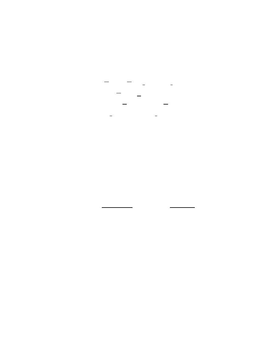
Therefore, the theory we will consider is
L = L
0
+
L
1
,
(621)
L
0
= iΨ/
∂Ψ
− mΨΨ −
1
2
∂
µ
ϕ∂
µ
ϕ
−
1
2
M
2
ϕ
2
,
(622)
L
1
= iZ
g
gϕΨγ
5
Ψ
−
1
24
Z
λ
λϕ
4
+
L
ct
,
(623)
L
ct
= i(Z
Ψ
−1)Ψ/∂Ψ − (Z
m
−1)mΨΨ
−
1
2
(Z
ϕ
−1)∂
µ
ϕ∂
µ
ϕ
−
1
2
(Z
M
−1)M
2
ϕ
2
(624)
where λ is a new coupling constant. We will use an on-shell renormalization
scheme. The lagrangian parameter m is then the actual mass of the electron.
We will define the couplings g and λ as the values of appropriate vertex
functions when the external four-momenta vanish. Finally, the fields are
normalized according to the requirements of the LSZ formula. In practice,
this means that the scalar and fermion propagators must have appropriate
poles with unit residue.
We will assume that M < 2m, so that the scalar is stable against decay
into an electron-positron pair. The exact scalar propagator (in momentum
space) can be then written in Lehmann-K¨all´en form as
˜
∆
(k
2
) =
1
k
2
+ M
2
− iǫ
+
Z
∞
M
2
th
ds ρ
ϕ
(s)
1
k
2
+ s
− iǫ
,
(625)
where the spectral density ρ
ϕ
(s) is real and nonnegative. The threshold mass
M
th
is either 2m (corresponding to the contribution of an electron-positron
pair) or 3M (corresponding to the contribution of three scalars; by parity,
there is no contribution from two scalars), whichever is less.
We see that ˜
∆
(k
2
) has a pole at k
2
=
−M
2
with residue one. This residue
corresponds to the field normalization that is needed for the validity of the
LSZ formula.
We can also write the exact scalar propagator in the form
˜
∆
(k
2
)
−1
= k
2
+ M
2
− iǫ − Π(k
2
) ,
(626)
where iΠ(k
2
) is given by the sum of one-particle irreducible (1PI for short;
see section 14) diagrams with two external scalar lines, and the external
128

propagators removed. The fact that ˜
∆
(k
2
) has a pole at k
2
=
−M
2
with
residue one implies that Π(
−M
2
) = 0 and Π
′
(
−M
2
) = 0; this fixes the
coefficients Z
ϕ
and Z
M
.
All of this is mimicked for the Dirac field. When parity is conserved, the
exact propagator (in momentum space) can be written in Lehmann-K¨all´en
form as
˜
S
(/
p) =
−/p + m
p
2
+ m
2
− iǫ
+
Z
∞
m
2
th
ds ρ
Ψ
(s)
−/p +
√
s
p
2
+ s
− iǫ
,
(627)
real and nonnegative. The threshold mass m
th
is m + M (corresponding to
the contribution of a fermion and a scalar), which, by assumption, is less
than 3m (corresponding to the contribution of three fermions; by Lorentz
invariance, there is no contribution from two fermions).
Since p
2
=
−/p/p, we can rewrite eq. (627) as
˜
S
(/
p) =
1
/
p + m
− iǫ
+
Z
∞
m
2
th
ds ρ
Ψ
(s)
1
/
p +
√
s
− iǫ
,
(628)
with the understanding that 1/(. . .) refers to the matrix inverse. However,
since /
p is the only matrix involved, we can think of ˜
S
(/
p) as an analytic
function of the single variable /
p. With this idea in mind, we see that ˜
S
(/
p)
has a pole at /
p =
−m with residue one. This residue corresponds to the field
normalization that is needed for the validity of the LSZ formula.
We can also write the exact fermion propagator in the form
˜
S
(/
p)
−1
= /
p + m
− iǫ − Σ(/p) ,
(629)
where iΣ(/
p) is given by the sum of 1PI diagrams with two external fermion
lines, and the external propagators removed. The fact that ˜
S
(/
p) has a pole
at /
p =
−m with residue one implies that Σ(−m) = 0 and Σ
′
(
−m) = 0; this
fixes the coefficients Z
Ψ
and Z
m
.
We proceed to the diagrams. The Yukawa vertex carries a factor of
i(iZ
g
g)γ
5
=
−Z
g
gγ
5
. Since Z
g
= 1 + O(g
2
), we can set Z
g
= 1 in the
one-loop diagrams.
Consider first Π(k
2
), which receives the one-loop (and counterterm) cor-
rections shown in fig. (12). The first diagram has a closed fermion loop. As
we will see in problem 51.1 (and section 53), anticommutation of the fermion
129
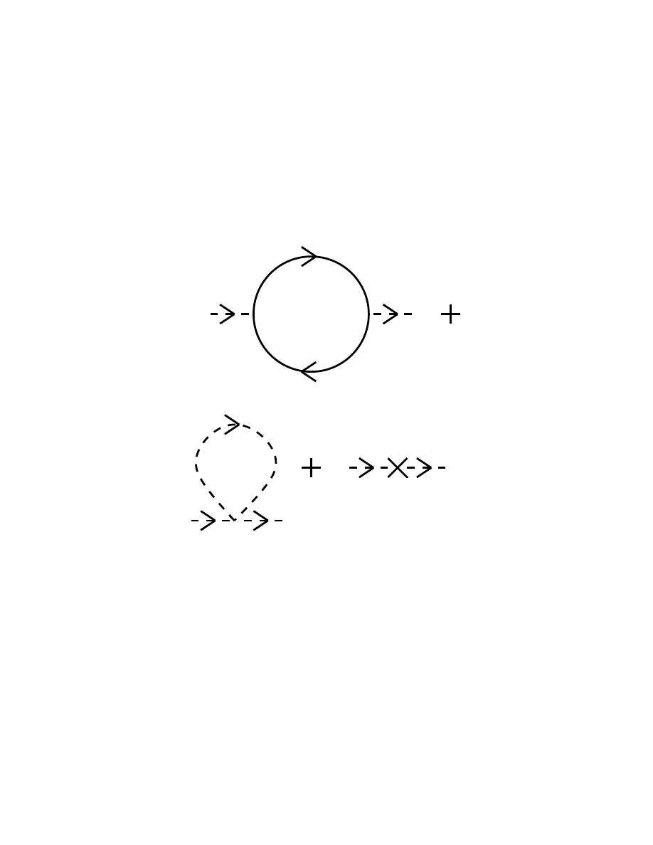
k
k
k
k
k
k
l
k+l
l
Figure 12: The one-loop and counterterm corrections to the scalar propagator
in Yukawa theory.
130

fields results in an extra factor of minus one for each closed fermion loop.
The spin indices on the propagators and vertices are contracted in the usual
way, following the arrows backwards. Since the loop closes on itself, we end
up with a trace over the spin indices. Thus we have
iΠ
Ψ loop
(k
2
) = (
−1)(−g)
2
1
i
2
Z
d
4
ℓ
(2π)
4
Tr
h
˜
S(/ℓ+/
k)γ
5
˜
S(/ℓ)γ
5
i
,
(630)
where
˜
S(/
p) =
−/p + m
p
2
+ m
2
− iǫ
(631)
is the free fermion propagator in momentum space.
We now proceed to evaluate eq. (630). We have
Tr[(
−/ℓ − /k + m)γ
5
(
−/ℓ + m)γ
5
] = Tr[(
−/ℓ − /k + m)(+/ℓ + m)]
= 4[(ℓ + k)ℓ + m
2
]
≡ 4N .
(632)
The first equality follows from γ
2
5
= 1 and γ
5
/
pγ
5
=
−/p.
Next we combine the denominators with Feynman’s formula. Suppressing
the iǫ’s, we have
1
(ℓ+k)
2
+ m
2
1
ℓ
2
+ m
2
=
Z
1
0
dx
1
(q
2
+ D)
2
,
(633)
where q = ℓ + xk and D = x(1
−x)k
2
+ m
2
.
We then change the integration variable in eq. (630) from ℓ to q; the result
is
iΠ
Ψ loop
(k
2
) = 4g
2
Z
1
0
dx
Z
d
4
q
(2π)
4
N
(q
2
+ D)
2
,
(634)
where now N = (q + (1
−x)k)(q − xk) + m
2
. The integral diverges, and so we
analytically continue it to d = 4
− ε spacetime dimensions. (Here we ignore
a subtlety with the definition of γ
5
in d dimensions, and assume that γ
2
5
= 1
and γ
5
/
pγ
5
=
−/p continue to hold.) We also make the replacement g → g˜µε
/2
,
where ˜
µ has dimensions of mass, so that g remains dimensionless.
131

Expanding out the numerator, we have
N = q
2
− x(1−x)k
2
+ m
2
+ (1
−2x)kq .
(635)
The term linear in q integrates to zero. For the rest, we use the general result
of section 14 to get
˜
µε
Z
d
d
q
(2π)
d
1
(q
2
+ D)
2
=
i
16π
2
2
ε
− ln(D/µ
2
)
,
(636)
˜
µε
Z
d
d
q
(2π)
d
q
2
(q
2
+ D)
2
=
i
16π
2
2
ε
+
1
2
− ln(D/µ
2
)
(
−2D) ,
(637)
where µ
2
= 4πe
−γ
˜
µ
2
, and we have dropped terms of order ε. Plugging
eqs. (636) and (637) into eq. (634) yields
Π
Ψ loop
(k
2
) =
−
g
2
4π
2
"
1
ε
(k
2
+ 2m
2
) +
1
6
k
2
+ m
2
−
Z
1
0
dx
3x(1
−x)k
2
+ m
2
ln(D/µ
2
)
#
.
(638)
We see that the divergent term has (as expected) a form that permits can-
cellation by the counterterms.
We evaluated the second diagram of fig. (12) in section 30, with the result
Π
ϕ loop
(k
2
) =
λ
(4π)
2
1
ε
+
1
2
−
1
2
ln(M
2
/µ
2
)
M
2
.
(639)
The third diagram gives the contribution of the counterterms,
Π
ct
(k
2
) =
−(Z
ϕ
−1)k
2
− (Z
M
−1)M
2
.
(640)
Adding up eqs. (638–640), we see that finiteness of Π(k
2
) requires
Z
ϕ
= 1
−
g
2
4π
2
1
ε
+ finite
,
(641)
Z
M
= 1 +
λ
16π
2
−
g
2
2π
2
m
2
M
2
!
1
ε
+ finite
,
(642)
132
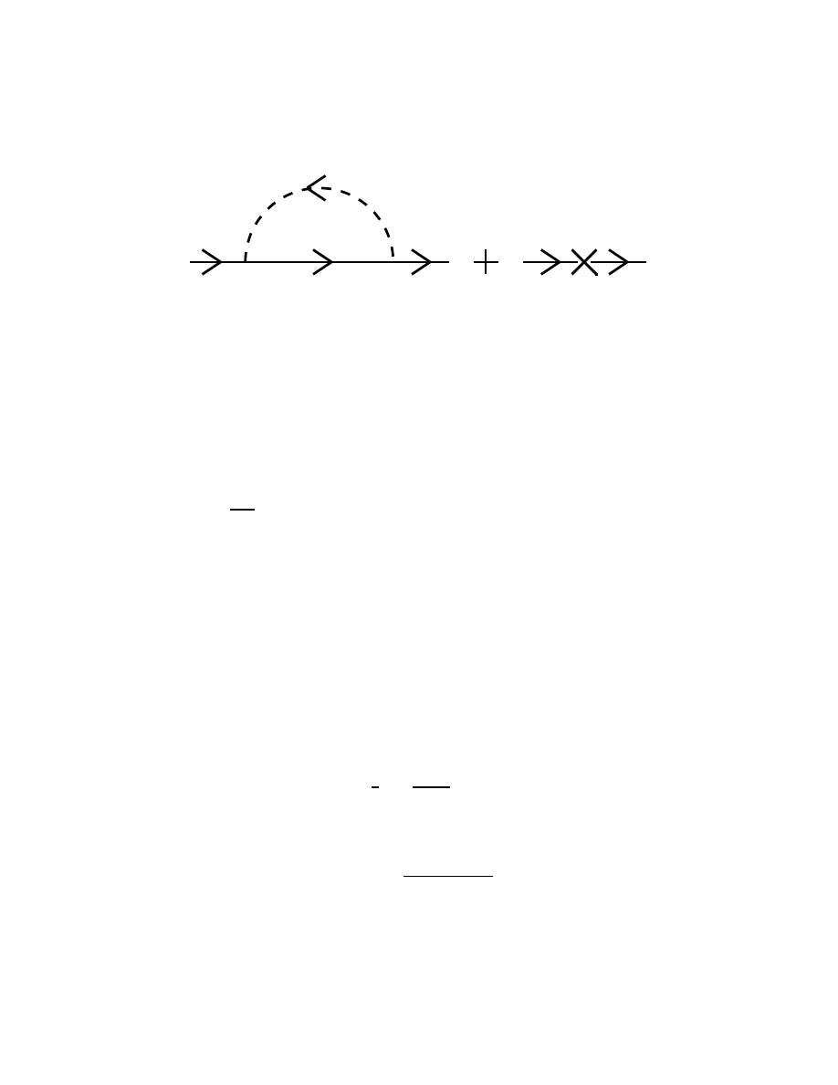
p
p
p
l
p
p+l
Figure 13: The one-loop and counterterm corrections to the fermion propa-
gator in Yukawa theory.
plus higher-order (in g and/or λ) corrections. Note that, although there is
an O(λ) correction to Z
M
, there is not an O(λ) correction to Z
ϕ
.
We can impose Π(
−M
2
) = 0 by writing
Π(k
2
) =
g
2
4π
2
Z
1
0
dx
3x(1
−x)k
2
+ m
2
ln(D/D
0
) + κ
Π
(k
2
+ M
2
)
, (643)
where D
0
=
−x(1−x)M
2
+ m
2
, and κ
Π
is a constant to be determined. We
fix κ
Π
by imposing Π
′
(
−M
2
) = 0, which yields
κ
Π
=
Z
1
0
dx x(1
−x)[3x(1−x)M
2
− m
2
]/D
0
.
(644)
Note that, in this on-shell renormalization scheme, there is no O(λ) correction
to Π(k
2
).
Next we turn to the Ψ propagator, which receives the one-loop (and
counterterm) corrections shown in fig. (13). The spin indices are contracted
in the usual way, following the arrows backwards. We have
iΣ
1 loop
(/
p) = (
−g)
2
1
i
2
Z
d
4
ℓ
(2π)
4
h
γ
5
˜
S(/
p + /ℓ)γ
5
i
˜
∆(ℓ
2
) ,
(645)
where ˜
S(/
p) is given by eq. (631), and
˜
∆(ℓ
2
) =
1
ℓ
2
+ M
2
− iǫ
(646)
is the free scalar propagator in momentum space.
133

We evaluate eq. (645) with the usual bag of tricks. The result is
iΣ
1 loop
(/
p) =
−g
2
Z
1
0
dx
Z
d
4
q
(2π)
4
N
(q
2
+ D)
2
,
(647)
where q = ℓ + xp and
N = /q + (1
−x)/p + m ,
(648)
D = x(1
−x)p
2
+ xm
2
+ (1
−x)M
2
.
(649)
The integral diverges, and so we analytically continue it to d = 4
−ε spacetime
dimensions, make the replacement g
→ g˜µε
/2
, and take the limit as ε
→ 0.
The term linear in q in eq. (648) integrates to zero. Using eq. (636), we get
Σ
1 loop
(/
p) =
−
g
2
16π
2
"
1
ε
(/
p + 2m)
−
Z
1
0
dx
(1
−x)/p + m
ln(D/µ
2
)
#
.
(650)
We see that the divergent term has (as expected) a form that permits can-
cellation by the counterterms, which give
Σ
ct
(/
p) =
−(Z
Ψ
−1)/p − (Z
m
−1)m .
(651)
Adding up eqs. (650) and (651), we see that finiteness of Σ(/
p) requires
Z
Ψ
= 1
−
g
2
16π
2
1
ε
+ finite
,
(652)
Z
m
= 1
−
g
2
8π
2
1
ε
+ finite
,
(653)
plus higher-order corrections.
We can impose Σ(
−m) = 0 by writing
Σ(/
p) =
g
2
16π
2
Z
1
0
dx
(1
−x)/p + m
ln(D/D
0
) + κ
Σ
(/
p + m)
,
(654)
where D
0
is D evaluated at p
2
=
−m
2
, and κ
Σ
is a constant to be determined.
We fix κ
Σ
by imposing Σ
′
(
−m) = 0. In differentiating with respect to /p, we
take the p
2
in D, eq. (649), to be
−/p
2
; we find
κ
Σ
=
−2
Z
1
0
dx x
2
(1
−x)m
2
/D
0
.
(655)
134
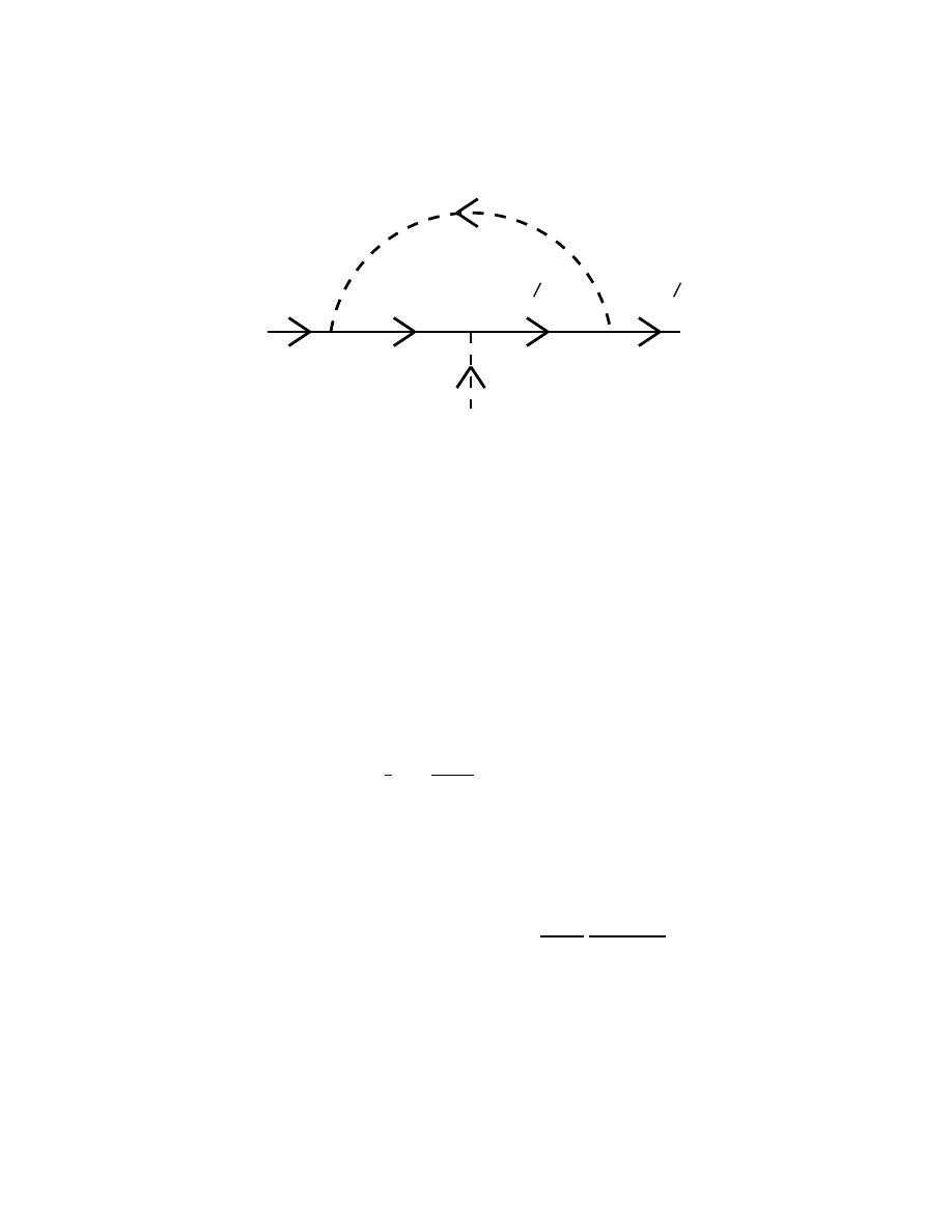
+l
l
p+l
p
p
k
p
Figure 14: The one-loop correction to the scalar-fermion-fermion vertex in
Yukawa theory.
Next we turn to the correction to the Yukawa vertex. We define the vertex
function iV
Y
(p
′
, p) as the sum of one-particle irreducible diagrams with one
incoming fermion with momentum p, one outgoing fermion with momentum
p
′
, and one incoming scalar with momentum k = p
′
− p. The original vertex
−Z
g
gγ
5
is the first term in this sum, and the diagram of fig. (14) is the second.
Thus we have
iV
Y
(p
′
, p) =
−Z
g
gγ
5
+ iV
Y, 1 loop
(p
′
, p) + O(g
5
) ,
(656)
where
iV
Y, 1 loop
(p
′
, p) = (
−g)
3
1
i
3
Z
d
d
ℓ
(2π)
d
h
γ
5
˜
S(/
p
′
+/ℓ)γ
5
˜
S(/
p+/ℓ)γ
5
i
˜
∆(ℓ
2
) . (657)
The numerator can be written as
N = (/
p
′
+ /ℓ + m)(
−/p − /ℓ + m)γ
5
,
(658)
and the denominators combined in the usual way. We then get
iV
Y, 1 loop
(p
′
, p)/g =
−ig
2
Z
dF
3
Z
d
4
q
(2π)
4
N
(q
2
+ D)
3
,
(659)
where the integral over Feynman parameters was defined in section 16, and
now
q = ℓ + x
1
p + x
2
p
′
,
(660)
135

N = [/q
− x
1
/
p + (1
−x
2
)/
p
′
+ m][
−/q − (1−x
1
)/
p + x
2
/
p
′
+ m]γ
5
,
(661)
D = x
1
(1
−x
1
)p
2
+ x
2
(1
−x
2
)p
′2
− 2x
1
x
2
p
·p
′
+ (x
1
+x
2
)m
2
+ x
3
M
2
. (662)
Using /q/q =
−q
2
, we can write N as
N = q
2
γ
5
+
f
N + (linear in q) ,
(663)
where
f
N = [
−x
1
/
p + (1
−x
2
)/
p
′
+ m][
−(1−x
1
)/
p + x
2
/
p
′
+ m]γ
5
.
(664)
The terms linear in q in eq. (663) integrate to zero, and only the first term is
divergent. Performing the usual manipulations, we find
iV
Y, 1 loop
(p
′
, p)/g =
−
g
2
8π
2
"
1
ε
−
1
4
−
1
2
Z
dF
3
ln(D/µ
2
)
γ
5
+
1
4
Z
dF
3
f
N
D
#
.
(665)
From eq. (656), we see that finiteness of V
Y
(p
′
, p) requires
Z
g
= 1 +
g
2
8π
2
1
ε
+ finite
,
(666)
plus higher-order corrections.
To fix the finite part of Z
g
, we need a condition to impose on V
Y
(p
′
, p).
One possibility is to mimic what we did in ϕ
3
theory in section 16: require
V
Y
(0, 0) to have the tree-level value igγ
5
. As in ϕ
3
theory, this is not well
motivated physically, but has the virtue of simplicity, and this is a good
enough reason for us to adopt it. We leave the details to problem 51.2.
Next we turn to the corrections to the ϕ
4
vertex iV
4
(k
1
, k
2
, k
3
, k
4
); the
tree-level contribution is
−iZ
λ
λ. There are diagrams with a closed fermion
loop, as shown in fig. (15), plus one-loop diagrams with ϕ particles only that
we evaluated in section 30. We have
iV
4, Ψ loop
= (
−1)(−g)
4
1
i
4
Z
d
4
ℓ
(2π)
4
Tr
h
˜
S(/ℓ)γ
5
˜
S(/ℓ
−/k
1
)γ
5
× ˜
S(/ℓ+/
k
2
+/
k
3
)γ
5
˜
S(/ℓ+/
k
2
)γ
5
i
+ 5 permutations of (k
2
, k
3
, k
4
) .
(667)
Again we can employ the standard methods; there are no unfamiliar aspects.
This being the case, let us concentrate on obtaining the divergent part; this
136
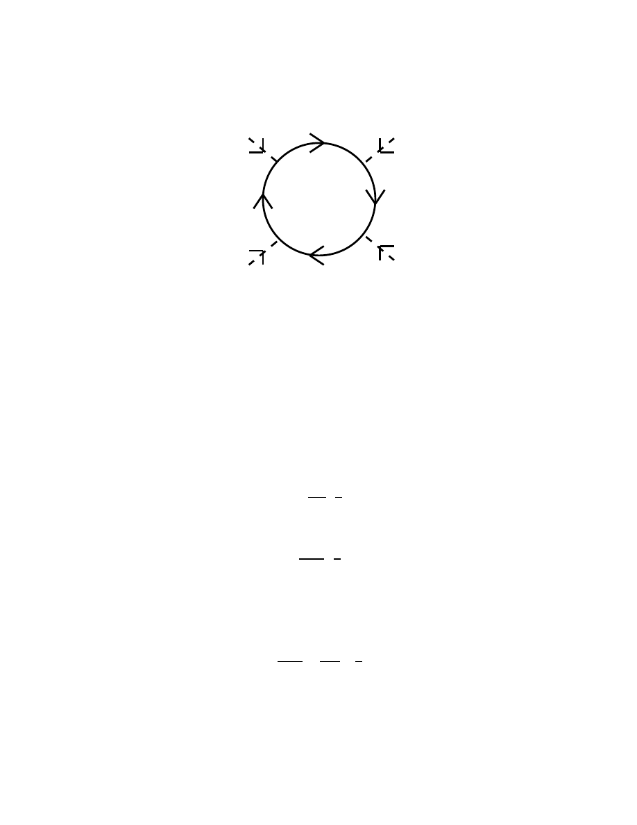
l
k
k
k
k
1
2
3
4
Figure 15: One of six diagrams with a closed fermion loop and four external
scalar lines; the other five are obtained by permuting the external momenta
in all possible inequivalent ways.
will give us enough information to calculate the one-loop contributions to
the beta functions for g and λ.
To obtain the divergent part of eq. (667), it is sufficient to set k
i
= 0.
Then the numerator in eq. (667) becomes simply Tr (/ℓγ
5
)
4
= 4(ℓ
2
)
2
, and
the denominator is (ℓ
2
+ m
2
)
4
. Then we find, after including the identical
contributions from the other five permutations of the external momenta,
V
4, Ψ loop
=
−
3g
4
π
2
1
ε
+ finite
.
(668)
From section 30, we have
V
4, ϕ loop
=
3λ
16π
2
1
ε
+ finite
.
(669)
Then, using
V
4
=
−Z
λ
λ + V
4, Ψ loop
+ V
4, ϕ loop
+ . . . ,
(670)
we see that finiteness of V
4
requires
Z
λ
= 1 +
3λ
16π
2
−
3g
4
π
2
λ
!
1
ε
+ finite
,
(671)
plus higher-order corrections.
137

Problems
51.1) Derive the one-loop correction to the scalar propagator by working
through eq. (475), and show that it has an extra minus sign (corresponding
to the closed fermion loop).
51.2) Prove eq. (627). Hints: Given a multiparticle state
|p, s, q, ni with
four momentum p
µ
and mass M
2
=
−p
2
, J
z
=
1
2
s, charge q, and other
attributes specified by n, show that
h0|Ψ(x)|p, s, q, ni vanishes unless s = ±1
and q = +1. Argue that this is enough information to fix
h0|Ψ(x)|p, s, q, ni ∝
u
s
(p), a spinor of mass M.
51.3) Finish the computation of V
Y
(p
′
, p), imposing the condition
V
Y
(0, 0) = igγ
5
.
(672)
138

Quantum Field Theory
Mark Srednicki
52: Beta Functions in Yukawa Theory
Prerequisite: 27, 51
In this section we will compute the beta functions for the Yukawa coupling
g and the ϕ
4
coupling λ in Yukawa theory, using the methods of section 27.
The relations between the bare and renormalized couplings are
g
0
= Z
−1/2
ϕ
Z
−1
Ψ
Z
g
˜
µε
/2
g ,
(673)
λ
0
= Z
−2
ϕ
Z
λ
˜
µελ .
(674)
Let us define
ln
Z
−1/2
ϕ
Z
−1
Ψ
Z
g
=
∞
X
n=1
G
n
(g, λ)
ε
n
,
(675)
ln
Z
−2
ϕ
Z
λ
=
∞
X
n=1
L
n
(g, λ)
ε
n
.
(676)
From our results in section 51, we have
G
1
(g, λ) =
5g
2
16π
2
+ . . . ,
(677)
L
1
(g, λ) =
3λ
16π
2
+
g
2
2π
2
−
3g
4
π
2
λ
+ . . . ,
(678)
where the ellipses stand for higher-order (in g
2
and/or λ) corrections.
Taking the logarithm of eqs. (673) and (674), and using eqs. (675) and
(676), we get
ln g
0
=
∞
X
n=1
G
n
(g, λ)
ε
n
+ ln g +
1
2
ε ln ˜
µ ,
(679)
ln λ
0
=
∞
X
n=1
L
n
(g, λ)
ε
n
+ ln λ + ε ln ˜
µ .
(680)
139

We now use the fact that g
0
and λ
0
must be independent of µ. We differenti-
ate eqs. (679) and (680) with respect to ln µ; the left-hand sides vanish, and
we multiply the right-hand sides by g and λ, respectively. The result is
0 =
∞
X
n=1
g
∂G
n
∂g
dg
d ln µ
+ g
∂G
n
∂λ
dλ
d ln µ
!
1
ε
n
+
dg
d ln µ
+
1
2
εg ,
(681)
0 =
∞
X
n=1
λ
∂L
n
∂g
dg
d ln µ
+ λ
∂L
n
∂λ
dλ
d ln µ
!
1
ε
n
+
dλ
d ln µ
+ ελ .
(682)
In a renormalizable theory, dg/d ln µ and dλ/d ln µ must be finite in the ε
→ 0
limit. Thus we can write
dg
d ln µ
=
−
1
2
εg + β
g
(g, λ) ,
(683)
dλ
d ln µ
=
−ελ + β
λ
(g, λ) .
(684)
Substituting these into eqs. (681) and (682), and matching powers of ε, we
find
β
g
(g, λ) = g
1
2
g
∂
∂g
+ λ
∂
∂λ
!
G
1
,
(685)
β
λ
(g, λ) = λ
1
2
g
∂
∂g
+ λ
∂
∂λ
!
L
1
.
(686)
The coefficients of all higher powers of 1/ε must also vanish, but this gives
us no more information about the beta functions.
Using eqs. (677) and (678) in eqs. (685) and (686), we get
β
g
(g, λ) =
5g
3
16π
2
+ . . . ,
(687)
β
λ
(g, λ) =
1
16π
2
3λ
2
+ 8λg
2
− 48g
4
+ . . . .
(688)
The higher-order corrections have extra factors of g
2
and/or λ.
140

Quantum Field Theory
Mark Srednicki
53: Functional Determinants
Prerequisite: 44, 45
In the section we will explore the meaning of the functional determinants
that arise when doing gaussian path integrals, either bosonic or fermionic. We
will be interested in situations where the path integral over one particular
field is gaussian, but generates a functional determinant that depends on
some other field. We will see how to relate this functional determinant to a
certain infinite set of Feynman diagrams. We will need the technology we
develop here to compute the path integral for nonabelian gauge theory in
section 70.
We begin by considering a theory of a complex scalar field χ with
L = −∂
µ
χ
†
∂
µ
χ
− m
2
χ
†
χ + gϕχ
†
χ ,
(689)
where ϕ is a real scalar background field. That is, ϕ(x) is treated as a fixed
function of spacetime. Next we define the path integral
Z(ϕ) =
Z
Dχ
†
Dχ e
i
R
d
4
x L
,
(690)
where we use the ǫ trick of section 6 to impose vacuum boundary conditions,
and the normalization Z(0) = 1 is fixed by hand.
Recall from section 44 that if we have n complex variables z
i
, then we
can evaluate gaussian integrals by the general formula
Z
d
n
z d
n
¯
z exp (
−i¯z
i
M
ij
z
j
)
∝ (det M)
−1
.
(691)
In the case of the functional integral in eq. (690), the index i on the integration
variable is replaced by the continuous spacetime label x, and the “matrix”
M becomes
M(x, y) = [
−∂
2
x
+ m
2
− gϕ(x)]δ
4
(x
− y) .
(692)
141

In order to apply eq. (691), we have to understand what it means to compute
the determinant of this expression.
To this end, let us first note that we can write M = M
0
f
M , which is
shorthand for
M(x, z) =
Z
d
4
y M
0
(x, y)
f
M(y, z) ,
(693)
where
M
0
(x, y) = (
−∂
2
x
+ m
2
)δ
4
(x
− y) ,
(694)
f
M (y, z) = δ
4
(y
− z) − g∆(y − z)ϕ(z) .
(695)
Here ∆(y
− z) is the Feynman propagator, which obeys
(
−∂
2
y
+ m
2
)∆(y
− z) = δ
4
(y
− z) .
(696)
After various integrations by parts, it is easy to see that eqs. (693–695) re-
produce eq. (692).
Now we can use the general matrix relation
det AB = det A det B
(697)
to conclude that
det M = det M
0
det
f
M .
(698)
The advantage of this decomposition is that M
0
is independent of the back-
ground field ϕ, and so the resulting factor of (det M
0
)
−1
in Z(ϕ) can simply
be absorbed into the overall normalization. Furthermore, we have
f
M = I
−G,
where
I(x, y) = δ
4
(x
− y)
(699)
is the identity matrix, and
G(x, y) = g∆(x
− y)ϕ(y) .
(700)
Thus, for ϕ(x) = 0, we have
f
M = I and so det
f
M = 1. Then, using eq. (691)
and the normalization condition Z(0) = 1, we see that for nonzero ϕ(x) we
must have simply
Z(ϕ) = (det
f
M )
−1
.
(701)
142

Next, we need the general matrix relation
det A = exp Tr ln A ,
(702)
which is most easily proven by remembering that the determinant and trace
are both basis independent, and then working in a basis where A is in Jordan
form (that is, all entries below the main diagonal are zero). Thus we can write
det
f
M = exp Tr ln
f
M
= exp Tr ln(I
− G)
= exp Tr
"
−
∞
X
n=1
1
n
G
n
#
.
(703)
Combining eqs. (701) and (703) we get
Z(ϕ) = exp
∞
X
n=1
1
n
Tr G
n
,
(704)
where
Tr G
n
= g
n
Z
d
4
x
1
. . . d
4
x
n
∆(x
1
−x
2
)ϕ(x
2
) . . . ∆(x
n
−x
1
)ϕ(x
1
) .
(705)
This is our final result for Z(ϕ).
To better understand what it means, we will rederive it in a different
way. Consider treating the gϕχ
†
χ term in
L as an interaction. This leads
to a vertex that connects two χ propagators; the associated vertex factor
is igϕ(x). According to the general analysis of section 9, we have Z(ϕ) =
exp iΓ(ϕ), where iΓ(ϕ) is given by a sum of connected diagrams. (We have
called the exponent Γ rather than W because it is naturally interpreted as a
quantum action for ϕ after χ has been integrated out.) The only diagrams we
can draw with these Feynman rules are those of fig. (16), with n insertions
of the vertex, where n
≥ 1. The diagram with n vertices has an n-fold
cyclic symmetry, leading to a symmetry factor of S = n. The factor of i
associated with each vertex is canceled by the factor of 1/i associated with
each propagator. Thus the value of the n-vertex diagram is
1
n
g
n
Z
d
4
x
1
. . . d
4
x
n
∆(x
1
−x
2
)ϕ(x
2
) . . . ∆(x
n
−x
1
)ϕ(x
1
) .
(706)
143
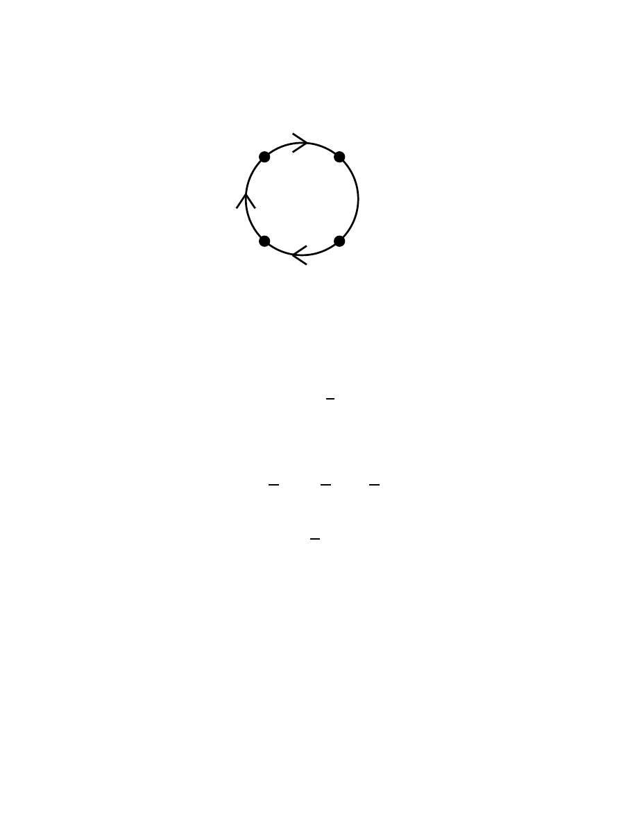
etc
Figure 16: All connected diagrams with ϕ(x) treated as an external field.
Each of the n dots represents a factor of igϕ(x), and each solid line is a χ or
Ψ propagator.
Summing up these diagrams, and using eq. (705), we find
iΓ(ϕ) =
∞
X
n=1
1
n
Tr G
n
.
(707)
This neatly reproduces eq. (704). Thus we see that a functional determinant
can be represented as an infinite sum of Feynman diagrams.
Next we consider a theory of a Dirac fermion Ψ with
L = iΨ/∂Ψ − mΨΨ + gϕΨΨ ,
(708)
where ϕ is again a real scalar background field. We define the path integral
Z(ϕ) =
Z
DΨ DΨ e
i
R
d
4
x L
,
(709)
where we again use the ǫ trick to impose vacuum boundary conditions, and
the normalization Z(0) = 1 is fixed by hand.
Recall from section 44 that if we have n complex Grassmann variables
ψ
i
, then we can evaluate gaussian integrals by the general formula
Z
d
n
¯
ψ d
n
ψ exp
−i ¯
ψ
i
M
ij
ψ
j
∝ det M .
(710)
In the case of the functional integral in eq. (709), the index i on the integration
variable is replaced by the continuous spacetime label x plus the spinor index
144

α, and the “matrix” M becomes
M
αβ
(x, y) = [
−i/∂
x
+ m
− gϕ(x)]
αβ
δ
4
(x
− y) .
(711)
In order to apply eq. (710), we have to understand what it means to compute
the determinant of this expression.
To this end, let us first note that we can write M = M
0
f
M , which is
shorthand for
M
αγ
(x, z) =
Z
d
4
y M
0αβ
(x, y)
f
M
βγ
(y, z) ,
(712)
where
M
0αβ
(x, y) = (
−i/∂
x
+ m)
αβ
δ
4
(x
− y) ,
(713)
f
M
βγ
(y, z) = δ
βγ
δ
4
(y
− z) − gS
βγ
(y
− z)ϕ(z) .
(714)
Here S
βγ
(y
− z) is the Feynman propagator, which obeys
(
−i/∂
y
+ m)
αβ
S
βγ
(y
− z) = δ
αγ
δ
4
(y
− z) .
(715)
After various integrations by parts, it is easy to see that eqs. (712–714) re-
produce eq. (711).
Now we can use eq. (698). The advantage of this decomposition is that
M
0
is independent of the background field ϕ, and so the resulting factor
of det M
0
in Z(ϕ) can simply be absorbed into the overall normalization.
Furthermore, we have
f
M = I
− G, where
I
αβ
(x, y) = δ
αβ
δ
4
(x
− y)
(716)
is the identity matrix, and
G
αβ
(x, y) = gS
αβ
(x
− y)ϕ(y) .
(717)
Thus, for ϕ(x) = 0, we have
f
M = I and so det
f
M = 1. Then, using eq. (710)
and the normalization condition Z(0) = 1, we see that for nonzero ϕ(x) we
must have simply
Z(ϕ) = det
f
M .
(718)
145

Next, we use eqs. (703) and (718) to get
Z(ϕ) = exp
−
∞
X
n=1
1
n
Tr G
n
,
(719)
where now
Tr G
n
= g
n
Z
d
4
x
1
. . . d
4
x
n
tr S(x
1
−x
2
)ϕ(x
2
) . . . S(x
n
−x
1
)ϕ(x
1
) ,
(720)
and “tr” denotes a trace over spinor indices. This is our final result for Z(ϕ).
To better understand what it means, we will rederive it in a different
way. Consider treating the gϕΨΨ term in
L as an interaction. This leads
to a vertex that connects two Ψ propagators; the associated vertex factor
is igϕ(x). According to the general analysis of section 9, we have Z(ϕ) =
exp iΓ(ϕ), where iΓ(ϕ) is given by a sum of connected diagrams. (We have
called the exponent Γ rather than W because it is naturally interpreted as a
quantum action for ϕ after Ψ has been integrated out.) The only diagrams we
can draw with these Feynman rules are those of fig. (16), with n insertions
of the vertex, where n
≥ 1. The diagram with n vertices has an n-fold
cyclic symmetry, leading to a symmetry factor of S = n. The factor of i
associated with each vertex is canceled by the factor of 1/i associated with
each propagator. The closed fermion loop implies a trace over the spinor
indices. Thus the value of the n-vertex diagram is
1
n
g
n
Z
d
4
x
1
. . . d
4
x
n
tr S(x
1
−x
2
)ϕ(x
2
) . . . S(x
n
−x
1
)ϕ(x
1
) .
(721)
Summing up these diagrams, we find that we are missing the overall minus
sign in eq. (719). The appropriate conclusion is that we must associate an
extra minus sign with each closed fermion loop.
146
Wyszukiwarka
Podobne podstrony:
Modanese Inertial Mass and Vacuum Fluctuations in Quantum Field Theory (2003)
Seahra S Path integrals in quantum field theory (web draft, 2002)(36s) PQft
Alvarez Gaume L , Introductory Lectures on Quantum Field Theory
Vol 3 Ch 06 Spin One Half
Norbury Quantum field theory (Wisconsin lecture notes, 2000)(107s)
Quantum field theory
CJ sight in black squares in squares upto 6 inch sq with one half inch grid upto 300yd
CJ 1 inch white circles in 1 5 inch black squares x 9 with one half inch grid lines
CJ sight in gray diamond in diamond & bars target with one half inch grid lines
Classical Field Theory Janos Polonoi
Field M , Nicol M Ergodic theory of equivariant diffeomorphisms (web draft, 2004)(94s) PD
An Introduction to Conformal Field Theory [jnl article] M Gaberdiel (1999) WW
więcej podobnych podstron