
PATRAN Beginner’s Guide
Arul M Britto
November 25, 2003
Contents
1
Introduction
3
2
How to Start a PATRAN Session
3
2.1
Creating a New Database . . . . . . . . . . . . . . . . . . . . . . . . . . . . . . . . . . . .
6
2.2
Opening New Database . . . . . . . . . . . . . . . . . . . . . . . . . . . . . . . . . . . . .
6
2.3
Leaving a PATRAN Session . . . . . . . . . . . . . . . . . . . . . . . . . . . . . . . . . . .
8
2.4
Resuming a Previous Session . . . . . . . . . . . . . . . . . . . . . . . . . . . . . . . . . .
9
3
Steps Involved in an analysis
9
3.1
Units . . . . . . . . . . . . . . . . . . . . . . . . . . . . . . . . . . . . . . . . . . . . . . . .
10
4
Create Geometry
10
4.1
Geometry . . . . . . . . . . . . . . . . . . . . . . . . . . . . . . . . . . . . . . . . . . . . . .
11
4.1.1
Create Points . . . . . . . . . . . . . . . . . . . . . . . . . . . . . . . . . . . . . . .
14
4.1.2
Create Curves . . . . . . . . . . . . . . . . . . . . . . . . . . . . . . . . . . . . . . .
14
4.2
Checking and Correcting Mistakes . . . . . . . . . . . . . . . . . . . . . . . . . . . . . . .
18
4.2.1
Check the Points . . . . . . . . . . . . . . . . . . . . . . . . . . . . . . . . . . . . .
18
4.2.2
Check the Curves . . . . . . . . . . . . . . . . . . . . . . . . . . . . . . . . . . . .
20
4.2.3
Deleting Points and Curves . . . . . . . . . . . . . . . . . . . . . . . . . . . . . . .
20
4.3
Error and Warning Messages . . . . . . . . . . . . . . . . . . . . . . . . . . . . . . . . . .
21
4.4
Entity Labels . . . . . . . . . . . . . . . . . . . . . . . . . . . . . . . . . . . . . . . . . . . .
21
4.5
Checking the Surface Normal . . . . . . . . . . . . . . . . . . . . . . . . . . . . . . . . . .
21
5
Loads and Boundary Conditions
23
5.1
Define the Load variation function . . . . . . . . . . . . . . . . . . . . . . . . . . . . . . .
23
5.2
Loads and Boundary Conditions . . . . . . . . . . . . . . . . . . . . . . . . . . . . . . . .
24
5.3
Load Application . . . . . . . . . . . . . . . . . . . . . . . . . . . . . . . . . . . . . . . . .
27
6
Define Element Properties
27
6.1
Define Material Properties . . . . . . . . . . . . . . . . . . . . . . . . . . . . . . . . . . . .
27
6.2
Element Properties . . . . . . . . . . . . . . . . . . . . . . . . . . . . . . . . . . . . . . . .
29
7
Finite Element Mesh
31
7.1
Create Mesh Seeds . . . . . . . . . . . . . . . . . . . . . . . . . . . . . . . . . . . . . . . .
31
7.2
Create the Mesh . . . . . . . . . . . . . . . . . . . . . . . . . . . . . . . . . . . . . . . . . .
33
7.3
Unpost the Geometry . . . . . . . . . . . . . . . . . . . . . . . . . . . . . . . . . . . . . . .
33
7.4
Equivalence and Optimize . . . . . . . . . . . . . . . . . . . . . . . . . . . . . . . . . . . .
34
8
Check Load/BCs
35
8.1
Loads/BCs . . . . . . . . . . . . . . . . . . . . . . . . . . . . . . . . . . . . . . . . . . . . .
36
8.2
Create a Load Case . . . . . . . . . . . . . . . . . . . . . . . . . . . . . . . . . . . . . . . .
37
1

CONTENTS
CONTENTS
9
Perform the Analysis
37
9.1
Submit a ABAQUS Analysis . . . . . . . . . . . . . . . . . . . . . . . . . . . . . . . . . . .
37
9.2
Accessing the ABAQUS Results from PATRAN . . . . . . . . . . . . . . . . . . . . . . . .
40
9.3
Post Processing . . . . . . . . . . . . . . . . . . . . . . . . . . . . . . . . . . . . . . . . . .
42
9.4
Changing Display Parameters . . . . . . . . . . . . . . . . . . . . . . . . . . . . . . . . . .
43
9.5
Hard Copy of Plot . . . . . . . . . . . . . . . . . . . . . . . . . . . . . . . . . . . . . . . . .
44
9.6
Stress Fringe Plot . . . . . . . . . . . . . . . . . . . . . . . . . . . . . . . . . . . . . . . . .
46
9.7
Using Graph (XY) Plot to plot Stress variation . . . . . . . . . . . . . . . . . . . . . . . . .
46
9.8
To Quit from PATRAN . . . . . . . . . . . . . . . . . . . . . . . . . . . . . . . . . . . . . .
47
10 Files
47
11 Troubleshooting
48
12 Frequently Asked Questions
49
2

2 HOW TO START A PATRAN SESSION
1
Introduction
PATRAN is a pre and post processing package for the finite element program ABAQUS. In addition
it has the capability of finite element analysis. This manual has been prepared for users who want to
use ABAQUS for finite element analysis. It also describes how once the ABAQUS analysis is run one
could carry out some post processing.
This manual tells the user how to run PATRAN in the Teaching system. It also has an example prob-
lem on how to set up the data for an ABAQUS analysis using PATRAN. It explains how a ABAQUS
job can be submitted from within PATRAN and after the successful completion of the job how to use
the post processing facilities.
2
How to Start a PATRAN Session
Find a suitable terminal for running PATRAN. These are the X-terminals in the main area of the DPO,
the PC-based X-terminals at the East end of the DPO, and the PC-based X-terminals in the EIET Lab
(Inglis building).
1. Log in using your user ID and password.
2. Run a window manager (example : twm& ). This is recommended. It is useful in the sense that
the PATRAN windows can be moved around and scaled. Do not run start, fvwm or fvwm2.
3. Create a subdirectory and move to it.
Type mkdir patran (you need to do this only once.)
Type cd patran (you need to do this for each session.)
It is a good idea to re-start PATRAN in the directory in which the database resides. Even though
it is possible to start PATRAN in any directory and then change to the directory in which the
database is, it is not recommended. The reason is any new files created by PATRAN (example
session files) will be placed in the directory from which PATRAN was started.
If you do not know which is your current directory then type pwd. This will list the name of the
current working directory.
Some useful unix commands :
ls -l
- will list all the files in the current directory.
cd
- to return to your HOME directory.
rm
<
file-name
>
- to delete a file. Replace
<
file-name
>
with name of file to be deleted. Example
: rm bracket.dat
Here the subdirectory is called patran. All the PATRAN related files will be placed in this di-
rectory. When you start a session of PATRAN ensure that there is enough unused disk space
available within your quota to complete the current exercise. Contact the Computer Operators if
you require the quota to be increased.
Alternatively you can work in the /tmp directory. However files created in the /tmp directory
are deleted automatically after 48 hours. Therefore if you require these files please copy them to
your home directory within that time. First check whether there is enough free disk space. If the
free disk space is less than 10 Mbytes do not use the /tmp directory.
Type bdf /tmp
Check the amount available under the heading avail. This will be in KBytes.
Type cd /tmp
Type mkdir
<
userid
>
. Here substitute your user-id for
<
userid
>
.
Type cd
<
userid
>
to move to this directory.
If you start PATRAN from here then all the files created will be placed in this directory.
3
2 HOW TO START A PATRAN SESSION
Show
Reset graphics
Undo
Refresh graphics
Heartbeat
Labels
Hide
Labels
Front
View
Interrupt
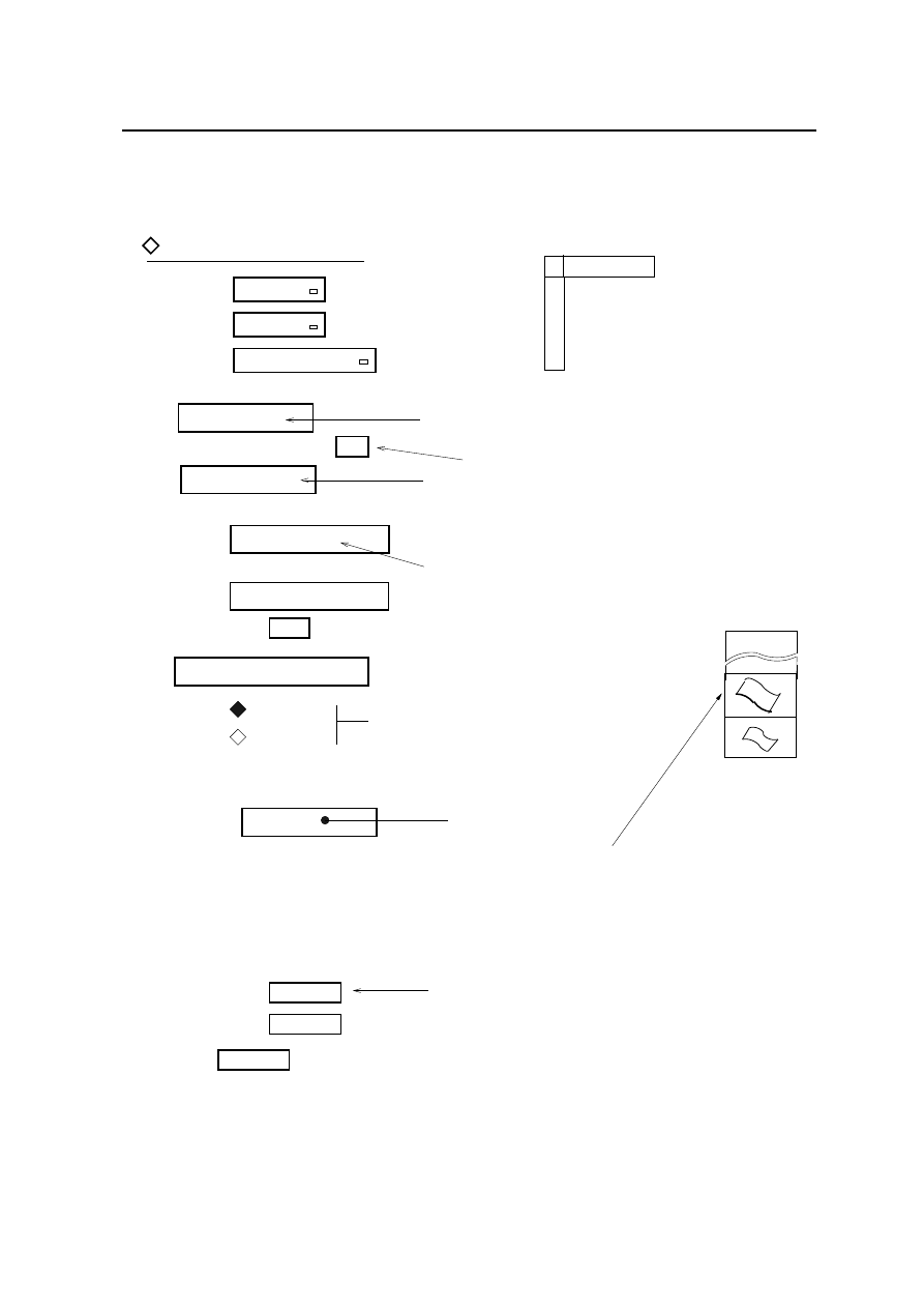
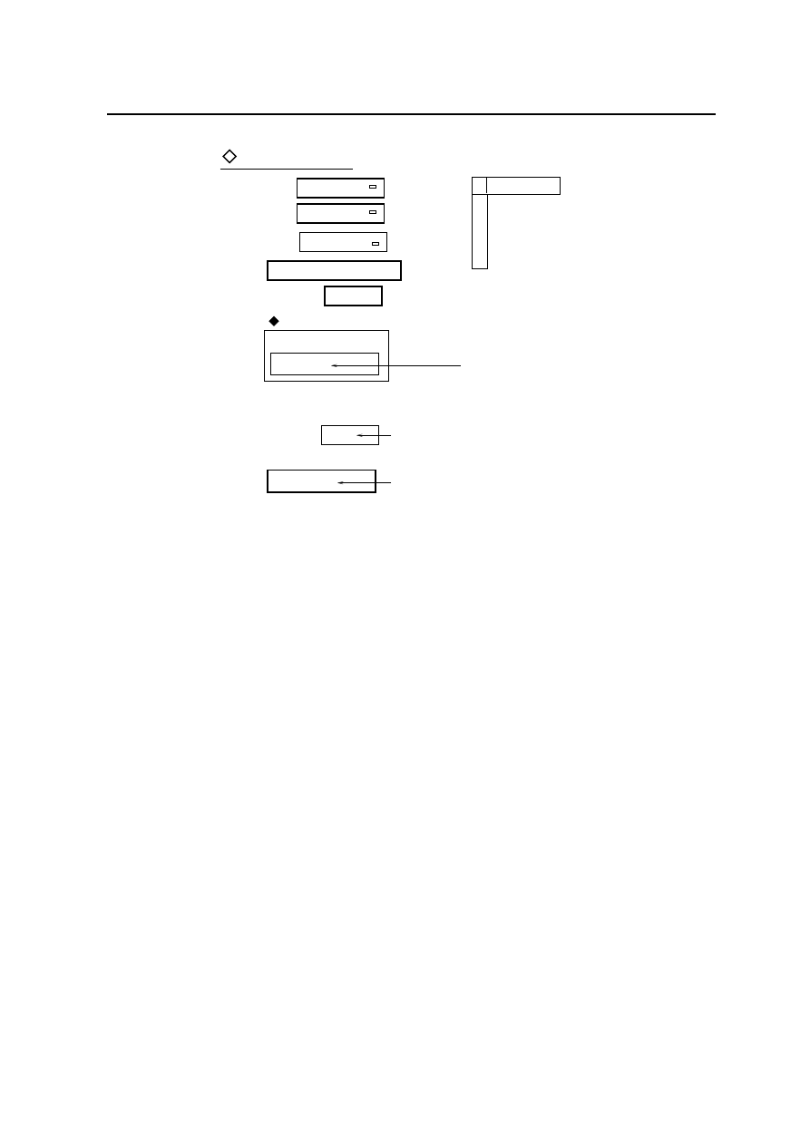
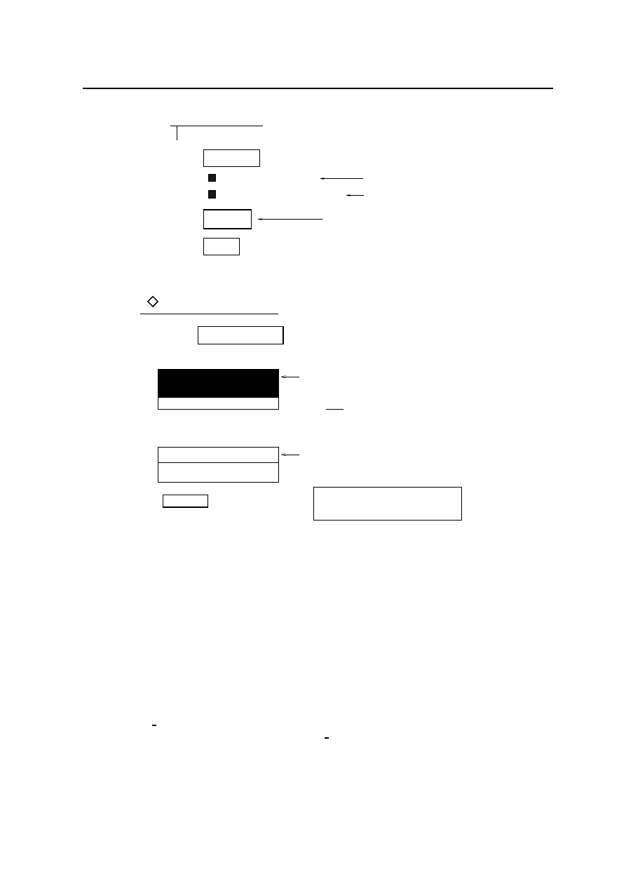
Figure 1: Main Form
4. Type patran (Note : must be in lower case)
Warning
Warning : Do not use the start or fvwm window manager or any of its derivatives
(fvwm2). In the past some problems have been encountered while running PATRAN with
fvwm.
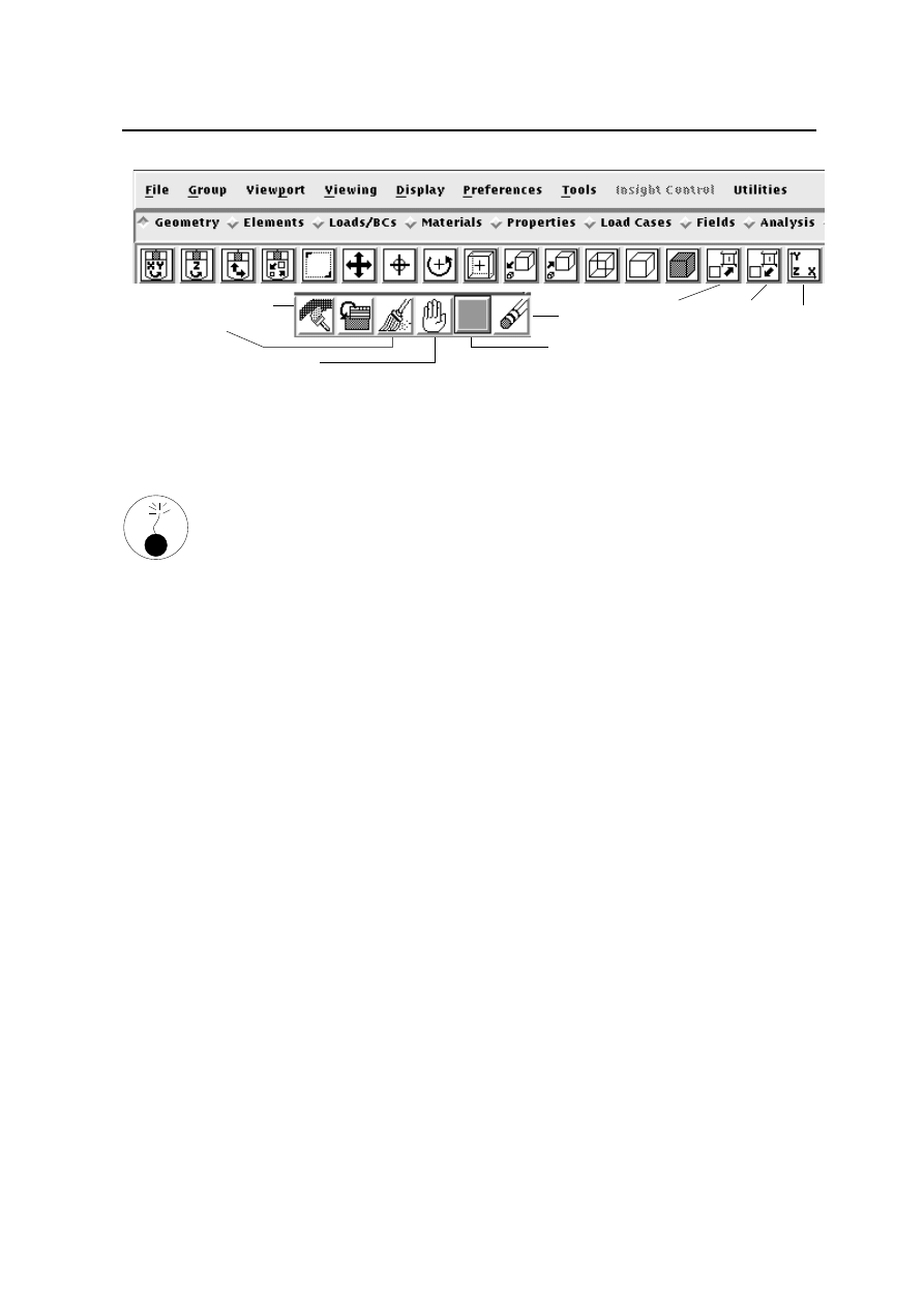
The MSC/PATRAN Main form (Figure 1, also see Appendix A, page 3) should appear
across the top of the screen.
At the top of the main form are
1. the pull-down menus, the on-line help, system icon buttons and the heartbeat.
Below that are
2. the application radio buttons
3. the toolbar icons
4. the history window area
5. the text command line
in that order (See Figure A1, in Appendix A).
The following message should appear in the history window :
MSC.PATRAN 2003 r2 has obtained 1 concurrent license(s) from FLEXlm ....
Then all is well. The MSC/PATRAN status indicator is displayed between the “interrupt” and
“undo” icons. This is the “ heartbeat”.
1. Green means ready and waiting.
2. Blue means busy, but can be interrupted.
3. Red means busy but not interruptible.
However if you get a message saying that PATRAN could not get a licence then try typing patran
again. If you still get the same message please contact the Computer Operators (operators@eng.cam.ac.uk)
and they should be able to sort out the problem.
If the licence was obtained successfully then wait for the heartbeat to turn Green. Only the ‘File’
command along the top row will appear in black. At this point that is the only command that can be
selected. The rest of the menus are greyed out.
In the rest of this document the actions to be taken by the user for completing the exercise is denoted
by the symbol
.
Before starting the exercise
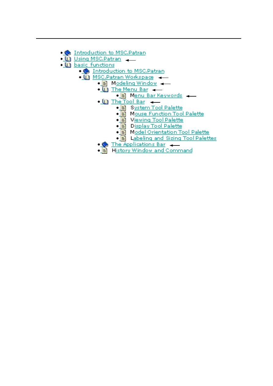
Click on Help from the top menu and choose ‘Contents and Index...’.
This would list the following headers.
4
2 HOW TO START A PATRAN SESSION
4
7
2
3
6
5
1
Figure 2: On-line Help Document
–
Introduction to MSC.Patran
–
Using MSC.Patran
–
Interfaces
–
Modules
–
PCL
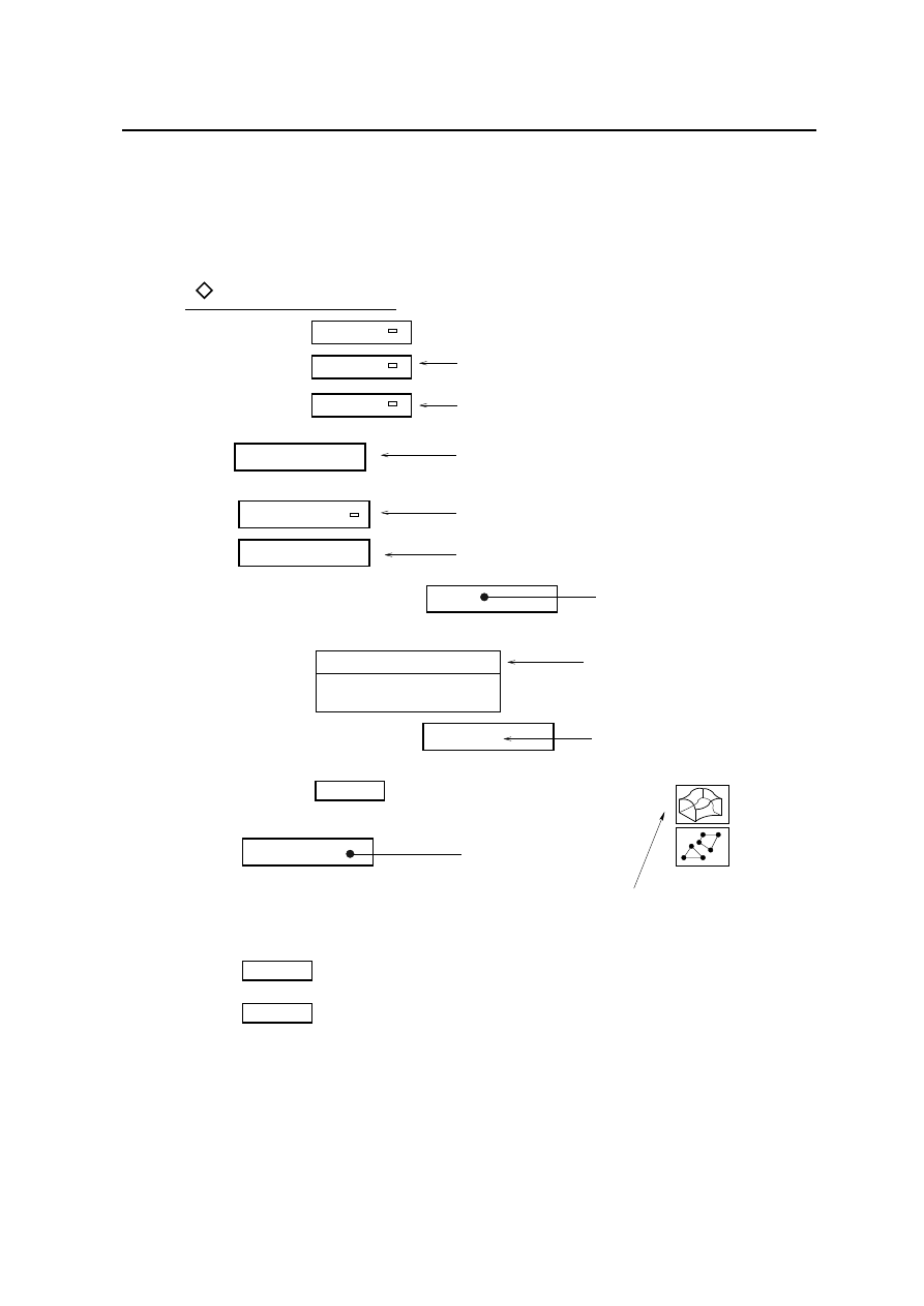
The selections to be made are indicated by numbered arrows in Figure 2,
Click on the “(Closed) Book” symbol or on the label “Using MSC.Patran”. This will open up and
display the subheadings. Then click on “MSC.Patran Workspace”.
Choose ‘Modelling Window’ from this menu (2 pages). This shows the Main form and the
Graphics viewport. Part of the Main form is shown in Figure 1.
Choose ‘Menu Bar’ and select ‘Menu Bar Keywords’. The items in the menu bar controls the
parameters of various system tasks. This page explains the keywords in the menu bar.
Below the Menu Bar is the Applications Bar. Below that is the Tool Bar. First we will consider the
Tool bar.
Click on ‘Tool Bar’ and this should display the various palettes that make up the tool bar. The
most frequently used icons are included in the Tool bar.
Figure 2
shows the contents page as it appears at this stage.
Next click on the ’Applications Bar’.
The essential work in using PATRAN is done by filling in the various forms in the ’Applications
Bar’.
Click on ‘Entering and Retrieving Data’ in the contents page.
This will list (a) Forms, Widgets and Buttons (6 pages) (b) Selecting Entities (6 pages).
These sections explain how to fill in the various forms. For the present just browse through these
pages. At this stage it is not essential reading for completing the exercise given in this handout.
However these are for future reference to be read later for becoming proficient with PATRAN.
5

2 HOW TO START A PATRAN SESSION
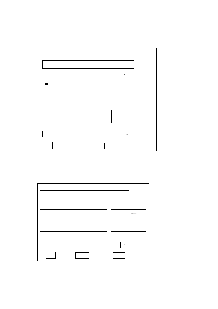
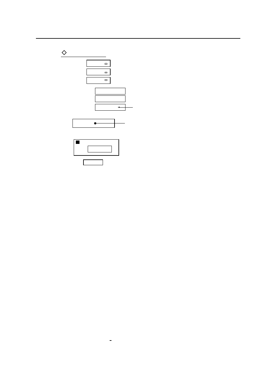
2.1 Creating a New Database
File
New ...
File should be the only menu selection
option that can be selected at this stage.
which is shown in black. This is the only
Remember, this is the top menu picked.
Figure 3: New database
The search facility is very useful. Also useful is the context-sensitive help available. When you
need more explanation on any form with a given setting leave the cursor on the form and then
press the F1 key. After a short pause this should display the relevant information from the on-line
help manual in a separate window. Once you have read the information close the help page.
Choose File / Quit to close the help page.
This way one should avoid any problem with continued use the F1 key.
2.1
Creating a New Database
Place the cursor on File and click the left mouse button.
Unless otherwise stated in the rest of this document it will be assumed that the left mouse button
is used for selecting menu options and items. The right mouse button is used for deselecting items; i.e.
if you make a mistake in selecting an item.
Choose from the menu the option New... (see Figure 3).
This will bring up a form which is shown in Figure 4. In this handout form in general means a
Dialogue box
.
2.2
Opening New Database
Click on the label marked ‘Change Template ...’.
This will open a new form (Figure 5).
To use ABAQUS then click on ‘abaqus.db’ from the list of available template files to select it.
Click on the OK button.
This will close that form.
Click on the box marked ‘New Database Name’ and type bracket and click on the OK button.
This is the name chosen for the current example.
The following messages should appear in the History window:
1. Copying /export/../patran2003r2/abaqus.db to bracket.db.
2. Template Copy complete.
3. Database version 3.1 created by Version 2003 r2 successfully opened.
4. Creating journal file bracket.db.jou at
<
date
><
time
>
.
Note that “.db” is automatically appended to the name. This denotes “database”. An empty view-
port should appear with a black background. The axes will be displayed. The cross hair symbol
represents the origin. The name of the database is displayed at the top of the viewport.
Appendix A contains a brief review of the notations used in PATRAN. It also explains the purpose
of the five icons (repaint, window layering, cleanup, abort and undo) displayed at the top right hand
corner.
When a new database is opened, the following form appears (see Figure 6).
6
2 HOW TO START A PATRAN SESSION
2.2 Opening New Database
Template Database Name
New Database
Filter
/amd_tmp/needle−16/usersn/userid/patran/*.db
Directories
Database List
Change Template ...
Click on this
.........................................../patran/.
.........................................../patran/..
bracket
OK
/export/../patran2003r2/template.db
Modify Preferences ...
Type
New Database Name
Cancel
Filter
bracket
Figure 4: New database
the box below :
Cancel
Filter
OK
Database Template
Template Name
/export/../patran2003r2/*.db
.........................................../patran/.
.........................................../patran/..
Database Template List
ABAQUS analysis.
abaqus.db
base.db
Click on this for
Directories
Filter
should appear in
Then this name
template.db
Figure 5: Change template
7
2 HOW TO START A PATRAN SESSION
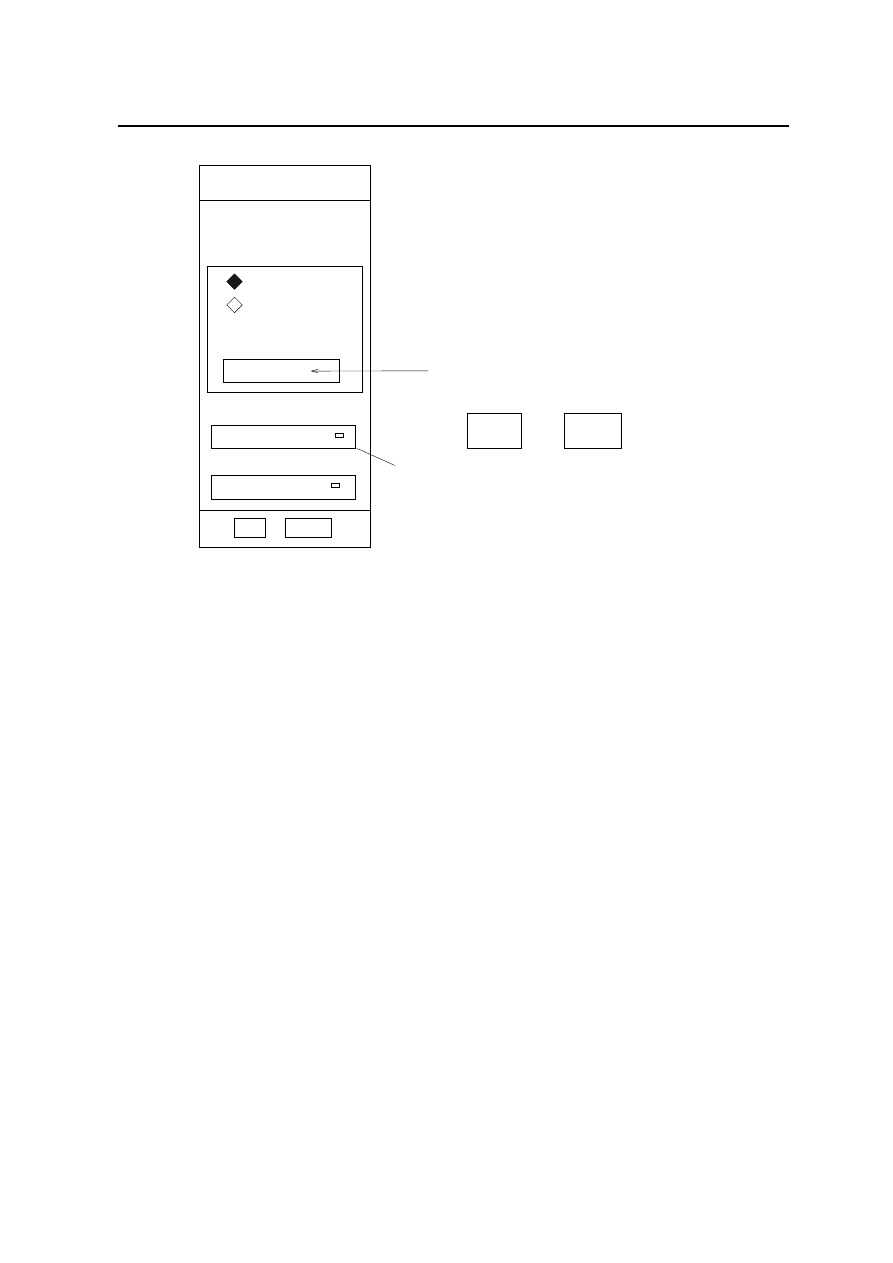
2.3 Leaving a PATRAN Session
New Model Preference
Model Preference for :
bracket.db
Tolerance
Analysis Code
Structural
Analysis Type :
This should display ABAQUS
Change this to 100.
10.0
Model Dimension :
Approximate Maximum
Use the
considered.
of the example problem being
This is the largest dimension
Default
based on Model
or
Delete
char
Reset
OK
key
characters
to delete
Delete
ABAQUS
Figure 6: Model Preference
Click on the box marked ‘Model Dimension’ and change the 10 to 100.
For the current example problem this is the largest dimension. The Tolerance parameter which
is used later is calculated based on this value. Therefore it is important to get this right approx-
imately. Getting this wrong can create a few problems later. The tolerance is taken as 0.0005 of
the largest dimension, so it will 0.05 for the current example. More on tolerance later.
Click on the OK button. This will close that form.
In general when entering/editing data in boxes in a form you need to click on the box first to
indicate to the program that you wish to do so. In the rest of this document when reference is made to
entering data in a box it will be assumed that you have to click on that box first even though this may
not be explicitly stated. Where there are exceptions to this rule it will be pointed out.
The next step is to create the geometry.
2.3
Leaving a PATRAN Session
You can quit the current session at any time you wish. Make sure that the heartbeat is green.
Then Click on the Quit button.
All the information input and actions taken are stored in the PATRAN database so there is no
need to save before quitting.
However if for some reason you want to save a copy of the database (for example to use it as a
template) then
Click on the File button Choose the Save a copy... option. Set the toggle to save a copy of the
journal file. Enter an appropriate name for the saved database.
Always save a copy of the journal file : *.db.jou (here * represents the name of the database).
Then wait for the Green light and choose the Quit option.
8

3 STEPS INVOLVED IN AN ANALYSIS
2.4 Resuming a Previous Session
Another situation where you may want to save a copy of the database is if you want to save the
results of the current analysis before making some changes (for example using a different element
type) and re-running the analysis and comparing the two sets of results. Then it will be a good idea to
work on a copy of the original database.
However you have to have enough spare disk space (quota) to be able to save a second copy of the
database.
First time users can skip the next section (section 2.3). It explains how to open an existing database
to continue a previous session.
2.4
Resuming a Previous PATRAN Session
Change to the directory where the the PATRAN database are present by typing ‘cd patran’.
Choose Open... instead of New... from the File menu.
Select the appropriate db file from the list of ‘available files’, by clicking on it.
That file name should appear in the box marked ‘Existing Database Name’.
Then click on the ‘OK’ button to choose that file.
It is recommended that you use separate databases for each new analysis.
If you want to look at a different PATRAN database then use File / Close to close the current
database and then open the other database.
3
Steps Involved in an analysis
The following is the order adopted for the various steps required for the current example.
1. Decide on what units to use
2. Create Geometry
3. Specify Boundary Conditions and Loading on the Geometry
4. Specify Material properties
5. Assign material properties to geometry
6. Create finite element mesh
7. Create a loadcase
8. Carry out the analysis
9. Read results
10. Post processing of the results
But one does not have to strictly adhere to this sequence. PATRAN provides flexibility. The user
can choose the sequence best suited for the problem in hand.
For example it is better to assign the material properties to the geometry rather than the finite
element mesh. This way if you decide to change the mesh you don’t have to re-assign the material
properties.
Similarly where necessary the specification of the boundary conditions or loading can be delayed
until after the mesh has been generated. In general boundary conditions and loading are specified in
the geometry.
The finite element mesh can be created immediately after the geometry has been created. But there
are good reasons to delay it.
9
4 CREATE GEOMETRY
3.1 Units
80 mm
20
80 mm
20 mm
100
z
y
x
75 mm
Figure 7: Example : L Bracket
3.1
Units
There is no default set of units assumed with ABAQUS. It is the user’s responsibility to choose an
appropriate set of units and enter all values using the correct units. For example the x co-ordinate of a
point is 20 mm. If you are using
m
for Length the value to be entered is 0.02. However if you are using
mm
for Length then you need to enter 20. The same applies to all numbers being entered which have
units associated with it.
From the PATRAN program’s point of view units doesn’t mean anything (all numerical entries are
just numbers). It means that all numerical input are treated as just numbers by PATRAN. For structural
problem the user should decide on the units for Length and Force. For time dependent problems the
unit for Time also has to be chosen. Example :
Length -
m
(metres)
Force -
N
(Newtons)
Time -
S
e
(seconds)
Then all dependent parameters must be specified in a consistent set of units. For example stiffness
should be specified in
N
=m
2
and density in
k
g
=m
3
.
For the example given here the SI(mm) units are used.
Quantity
SI
SI(mm)
SI
US Unit(ft)
US Unit(inch)
Length
m
mm
m
f
t
in
Force
N
N
k
N
l
bf
l
bf
Mass
k
g
tonne
(
10
3
k
g
)
tonne
sl
ug
l
bf
s
2
=in
Time
s
s
s
s
s
Stress
P
a
(N/
m
2
)
M
P
a
(N/
mm
2
)
k
P
a
l
bf
/
f
t
2
psi
(
l
bf
/
in
2
)
Energy
J
mJ
(
10
3
J)
K
J
f
tl
bf
inl
bf
Density
k
g
=m
3
tonne=mm
3
tonne=m
3
sl
ug
=f
t
3
lbf
s
2
=in
4
Note
Always choose your set of units before starting to create the geometry ie entering the
point co-ordinates. Because this affects the stiffness parameters, loading etc. This will
avoid unnecessary scaling of the results later.
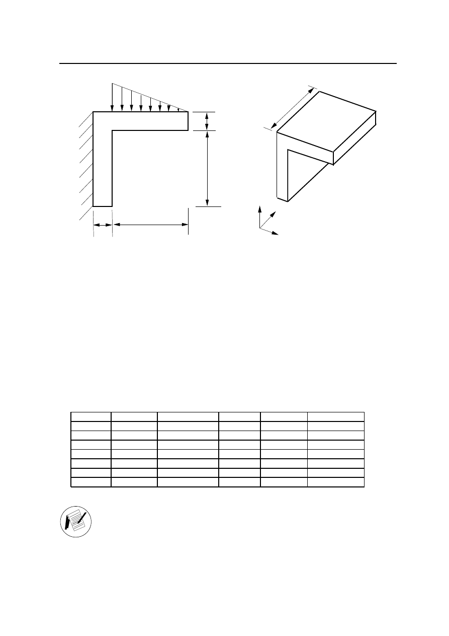
4
Create Geometry
The model is a simple L bracket which is fixed along one side (vertical) in both x and
y directions. Part of the other side (horizontal) is subjected to a triangular distribution
10

4 CREATE GEOMETRY
4.1 Geometry
1
1
2
3
4
Show Labels Icon
which varies from 100
N
=mm
2
to 0 at the tip (Figure 7). This is an elastic analysis and
contains a single load step. The analysis consists of a single increment. The SI(mm) units have been
chosen for the present example.
The bracket is 100 mm long along its side and is 20 mm thick and is 75 mm wide. This is to be
analysed as a Plane Stress problem.
Points, Curves and Surfaces and Solids (for 3D) form the Geometric Entity. The Nodes and Ele-
ments of the FE mesh form the FE Entities.
The bracket is to be divided into 3 surfaces. There are a number of ways to create a surface with
straight edges.
1. Create the 4 points and specify these as vertices and create a surface (Figure 8a).
2. Create the 4 edges of the surface using the above 4 points. Then use the 4 edges to create the
surface. This is the most tedious way to create a surface. But this is the only way to create a
surface if all 4 of its edges are curved (Figure 8b).
3. Create opposite edges of the surface and use these to create a surface. The 2 curves are joined
using straight lines in creating the surface (Figure 8c).
4. Create one curve (say) between points 1 and 2 and then extruded it in the Y direction to create
the surface (Figure 8d).
5. Use a single step to directly create the surface (XYZ Method). Here point 1 is chosen as one end
of the diagonal and then by specifying the diagonal vector the rectangle is created (Figure 8e).
Some of these methods of creating surfaces will be illustrated later.
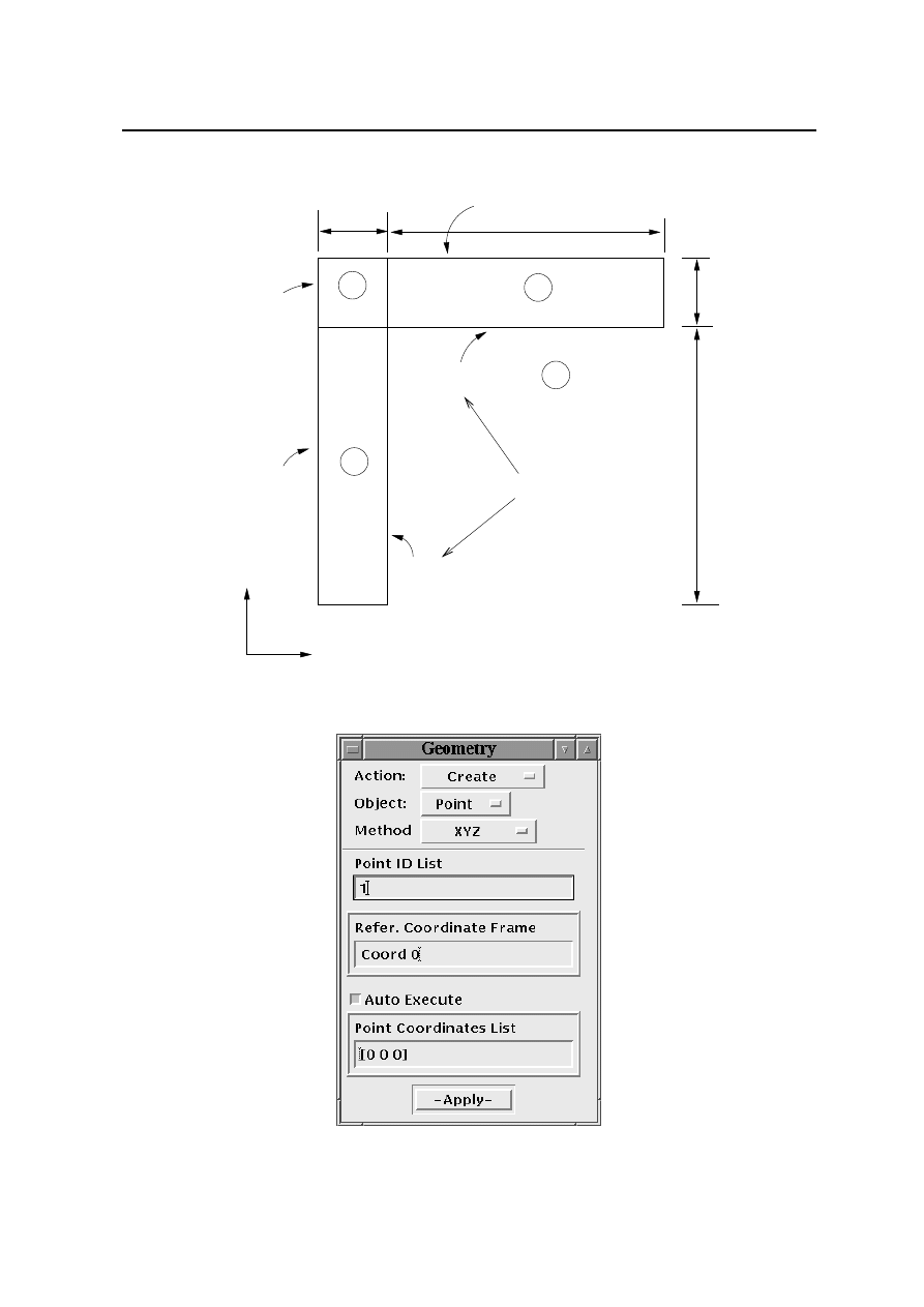
4.1
Geometry
Click on the Show labels icon from the Tool bar. This will display the point, curve numbers as
they are created later.
Click on the
3
Geometry
radio button.
This will open the geometry form and display it on the right hand side of the screen. Only one of
the forms indicated by the
3
symbol can be open at any given time. Clicking on the label of the form
which is currently open closes it. If you click on the label of another form the currently selected form
is closed and the new form is opened.
The Figure 9 shows the bracket divided into three surfaces. It is created using eight points and two
curves.
The geometry form is shown in Figure 10. You will also notice a column of icons with the heading
‘Pick’ displayed alongside the form. This is known as the Select Menu.
If you move the cursor from icon to icon in the select menu, text explaining each icon will pop up.
This is useful when picking entities. You choose an appropriate icon from this menu when needed.
The default icon is the first one (shown in reverse video ie highlighted). This icon means that the
coordinates of the points are directly entered. More on this later.
11
4 CREATE GEOMETRY
4.1 Geometry
2
1
1
1
2
1
4
3
2
4
Surface
Create
Curves
Surface
Create
Extrude
Surface
Create
XYZ
Create
Surface
b
c
d
e
Edges
Action : Create
Object : Surface
3
Create 4 points
Create 4 points
Create 4 points
Create 2 points
Create 1 curve
2
3
4
1
Create 4 curves
Create 4 curves
Translate
Curve
Method : Vertex
1
a
Figure 8: Different Ways of creating a surface
12
4 CREATE GEOMETRY
4.1 Geometry
Internal
80
20
Z
Y
X
3
3
5
2
1
1
1
2
6
surface 1.3
2
surface 2.1
surface 1.1
surface 3.4
surface 3.2
4
8
20
80
7
edges.
surface
of curves,
numbering
surface
Figure 9: L Bracket : The Surfaces
Figure 10: Geometry Form
13

4 CREATE GEOMETRY
4.1 Geometry
4.1.1 Create Points
The default setting of this form is for specifying directly the XYZ coordinates for the points. Notice the
2 boxes labelled ‘Point ID List’ and ‘Point Coordinates List’. The first point is to be placed at the origin.
Click on the Apply button to create the first point at the origin ( [0, 0, 0] ).
The point number is automatically incremented for the next point.
Click on the ‘Point Coordinates List’ and enter the coordinates 20 0 0 and click on the APPLY
button. Note that the co-ordinates are enclosed by square brackets ( [ ] ).
If you make any mistakes click on the ‘undo’ icon next the MSC label (top right hand corner, last
icon). This will undo the last command. In general, you can only undo the last command.
At this stage you could enter the co-ordinates [ 0 80 0 ] for the 3rd point and finally [ 20 80 0 ] for the
4th point co-ordinates, in order to create the first surface. However instead of that let us use a different
method to create the surface.
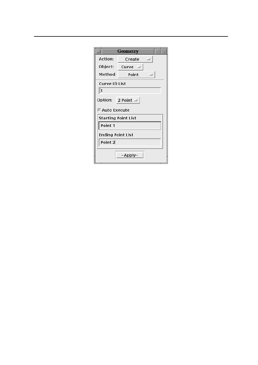
4.1.2 Create Curves
Change the ‘Object’ to ‘Curve’. This is done by pressing the left mouse button over ‘Point’ and
choosing ‘Curve’ by moving the mouse (while holding down the left mouse button) to that menu
option and releasing the mouse button.
Now check that the ‘Method’ is set to ‘Point’. The form should be as shown in Figure 11:
Notice the cursor (indicated by I) at the box marked‘ Starting Point List’. The bottom 2 boxes
where PATRAN expects data to be entered both deal with Points. Whichever point is selected
would be automatically placed in the first box marked ‘Starting Point List’.
Click on Point 1.
PATRAN now anticipates that the next selection will be the ’Ending Point’. So without clicking
on the box marked ‘Ending Point List’
click on the Point 2.
Now this label should appear in the 2nd box and without having to click on APPLY (because
AutoExecute is SET) the 1st Curve will be created and displayed. The curve and its label will be in
Yellow.
The entity selection (Selecting Point 2) for the last box acts as a trigger and executes the above
command.
First time users might find this a little disconcerting. The ‘Auto Execute’ button can be de-activated
by clicking on it. Then you need to click on APPLY to complete the action.
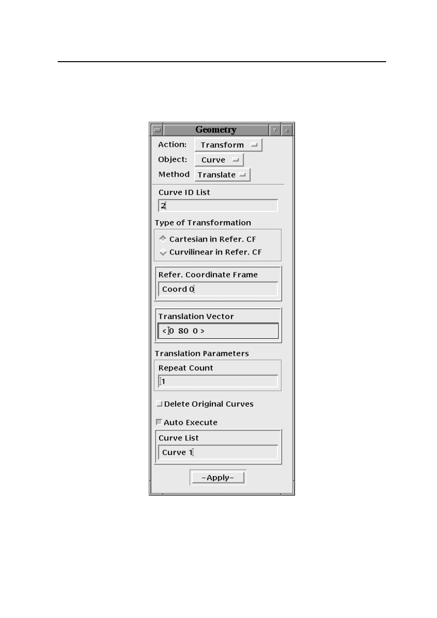
The next step is to create the Curve 2 by translating Curve 1.
Choose the Action : ‘Transform’ instead of ‘Create’.
Notice that the Curve ID List is displaying 2 in readiness for the next curve.
Change the ‘Object’ to ‘Curve’ and the ‘Method’ to ‘Translate’.
The form is as shown in Figure 12 :
The curve 2 is created by translating curve 1 in the y direction by 80 mms.
This is done by changing the ’Translation Vector’ to
<
0 80 0
>
.
14
4 CREATE GEOMETRY
4.1 Geometry
Figure 11: Constructing lines
Here DO NOT press the RETURN key after entering the ’Translation Vector’ because the form is
not complete. Otherwise a Window will appear with an error message. If it does click on OK to
acknowledge it in order to proceed.
Pressing the RETURN key in any of the boxes where the data are typed has the same effect as
executing the current task i.e. clicking on the APPLY button.
Therefore as a rule when typing in data refrain from pressing the RETURN key even if it is the last
box or entry which would complete the data input to that form.
This might lead to the tendency of pressing the RETURN key automatically whenever typing in
data in a box even when the form is not complete.
Leave the repeat count at 1, because we only require 1 curve to be created.
Click on the box marked ‘Curve List’ and then click on Curve 1. The Curve 2 will be displayed
without having to click on ‘APPLY’, if ‘Auto Execute’ is ON.
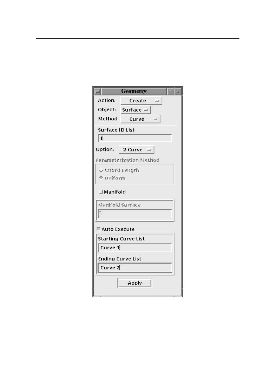
The next step is to create the surface using these 2 curves.
Change the ‘Action’ to ‘Create’. Change the ‘Object’ to ‘Surface’ and the ‘Method’ to ‘Curve’.
The form should be as shown in Figure 13:
Click on Curve 1.
PATRAN now anticipates that the next selection will be the Ending Curve. So without clicking
on the box marked ‘Ending Curve 2 List’
click on the Curve 2.
Now this label should appear in the 2nd box. At this point without having to click on APPLY (because
AutoExecute is SET) the 1st Surface will be created and displayed. The surface will be drawn in a
Green outline and its label will also be in Green.
Of course the conventional method of clicking on the boxes before making the selection still works.
Sometimes when mistakes are made use the ‘Undo’ icon and then follow the conventional method.
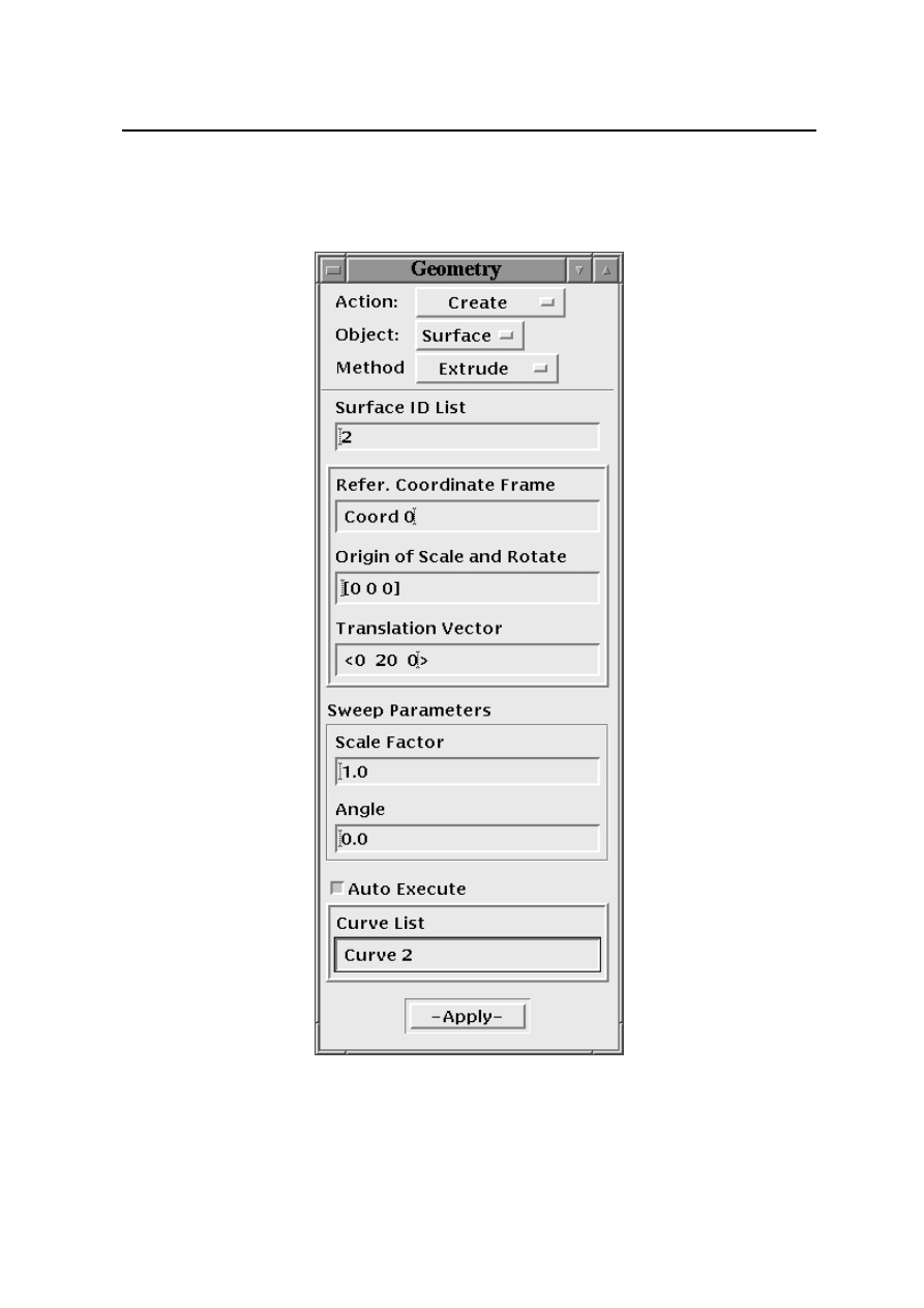
The next task is to create the second surface in a single step using the ‘Extrude Method’.
15
4 CREATE GEOMETRY
4.1 Geometry
Figure 12: Translate Curve
16
4 CREATE GEOMETRY
4.1 Geometry
Figure 13: Constructing a Surface from Curves
17

4 CREATE GEOMETRY
4.2 Checking and Correcting Mistakes
Leave the ‘Action’ at ‘Create’ and the ‘Object’ at ‘Surface’. Change the ‘Method’ to ‘Extrude’. The
form should be as shown in Figure 14:
Change the ‘Translation Vector’ to
<
0 20 0
>
.
Click in the box marked ‘Curve List’ and click on the ‘Curve 2’. This should create and draw the
surface in Green and display its number (Surface 2).
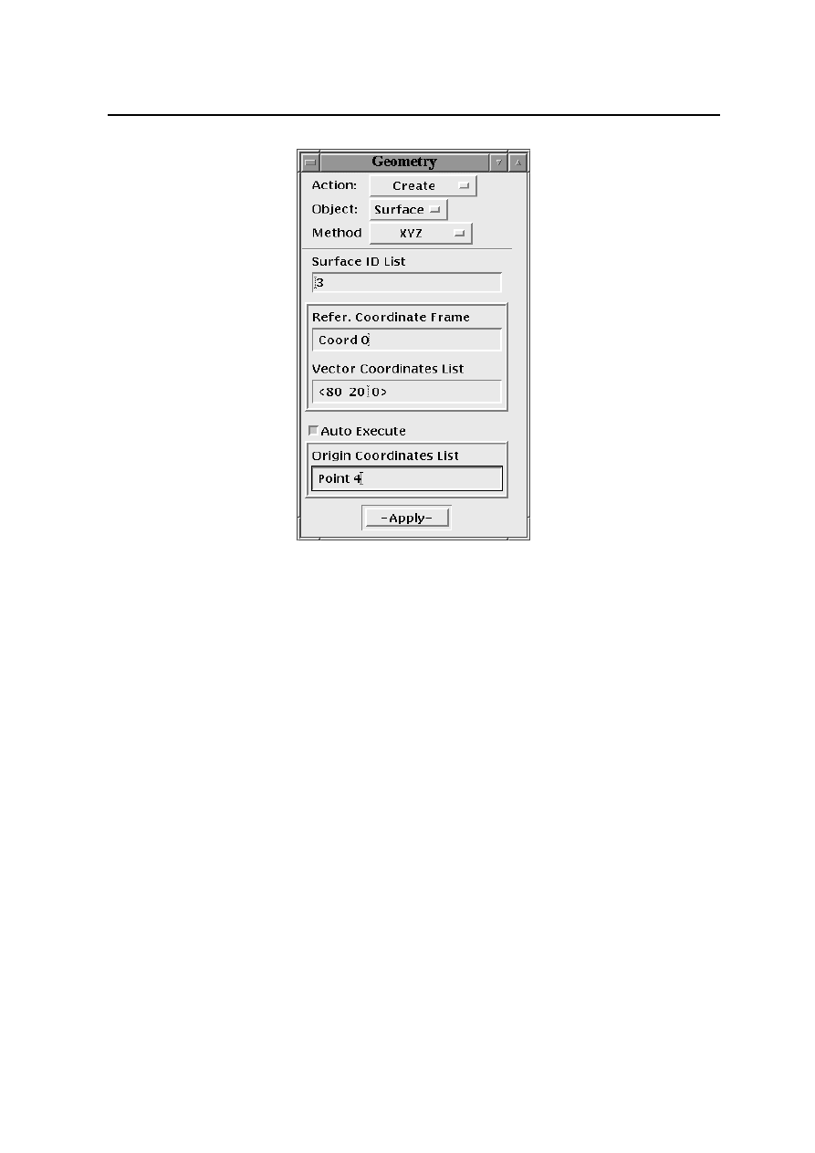
The next task is to create the third surface in a single step.
Leave the ‘Action’ at ‘Create’ and the ‘Object’ at ‘Surface’. Change the ‘Method’ to ‘XYZ’. The
form should be as shown in Figure 15:
Click on the second box (marked ‘Vector Coordinates List’) and then change it to
<
80 20 0
>
.
Leave the repeat count at 1, because only 1 surface is to be created.
Click in the box marked ‘Origin Coordinates List’ and then click on ‘Point 4’.
This should draw the surface in Green and display its number (Surface 3 ).
At this point you should have the 8 Points and 3 surfaces on the screen. However if you had made
mistakes you will find that you have more than 8 Points and/or 3 surfaces; do not panic. The next
section explains how mistakes can be detected and corrected. If there are no mistakes then skip to
section 4.3.
4.2
Checking and Correcting Mistakes
If you think that you have made no mistakes then skip the rest of this section (goto section 4.3).
Sometimes the mistakes made may be too many to be able to rectify it. Then it will be quicker to
delete everything and make a fresh start. For this
Change the ‘Action’ to ‘Delete’ and the ‘Object’ to ‘Any’.
Make sure that the ‘Autoexecute’ option is UNSET (In case you want to change your mind).
This is a drastic step. With a single action you are going to delete all Geometric entities (Points,
Curves, Surfaces). This warning is mainly for future reference when dealing with a more com-
plex/detailed situation. There is no going back. Here it is not that critical (if you make the wrong
choice)
Draw a box around all the entities in the viewport.
It should all change colour to light red.
Click on APPLY.
Otherwise the first thing to check is whether there are any duplicate points and lines.
4.2.1
Check the Points
Click on ‘Create’ label in the Geometry form and change it to ‘Show’.
Also change the other 2 options so that you have Show/Point/Location for Action/Object/Info.
The ‘Total in Model’ will display the total number of points that have been created. This should
be 8.
Click on the box marked ‘Point List’ and type ‘Point 1’, and click on ’Apply’.
This will display a form with the heading ‘Show Point Location Information’. Check that the
co-ordinates are correct for this point.
Repeat this procedure for the 2nd point.
Click on ‘Cancel’ to close that form.
The next section shows how to check the curve data.
18
4 CREATE GEOMETRY
4.2 Checking and Correcting Mistakes
Figure 14: Constructing a Surface Using the Extrude Method
19
4 CREATE GEOMETRY
4.2 Checking and Correcting Mistakes
Figure 15: Creating surface - XYZ method
4.2.2
Check the Curves
Change the options so that you have Show/Curve/Attributes for Action/Object/Info.
This will display the total number of lines that have been created.
Click on the box marked ‘Curve List’ and click on ‘Curve 1’.
This will display a form with the heading ‘Show Curve Attribute Information’. It will list the
Start and End Points. Check with figure 8 whether that information is correct.
Click on the ‘Cancel’ button on this form to close it.
Click on the box marked ‘Curve List’ and click on the ‘Curve 2’. Check the information for this line.
By now you should be able to identify any mistakes that have been made.
4.2.3 Deleting Points and Curves
If you need to delete any entities then do it in the reverse order these were created. For example to
delete points, curves and surfaces, delete the Surfaces first then the Curves and then finally the Points.
This is because of the dependency. Since the Surface creation is dependent on Curves and Points.
So if you try to delete such a Point then PATRAN will remind you of the dependence and ask whether
you want to delete the surface as well. To avoid these questions follow the order described.
If you need to delete any Curves then change the ‘Action’ to ‘Delete’. Change the ‘Object’ to
‘Curve’. Click on the box marked ‘Curve List’ and enter the line numbers you want to delete.
Then click on the ‘Apply’ button.
If you need to delete any points then change the ‘Action’ to ‘Delete’. The ‘Object’ will change to
‘Any’.
20

4 CREATE GEOMETRY
4.3 Error and Warning Messages
Click on ‘Any’ and change this to ‘Point’.
Click on the box marked ‘Point List’ and enter the point numbers you want to delete.
Then click on the ‘Apply’ button.
Make the necessary corrections and re-create any points, curves and surfaces so that the labels
match the ones in Figure 9. Otherwise cannot make progress with this exercise.
4.3
Error and Warning Messages
If you have made a mistake then PATRAN may put up an error message in a window. If an OK button
is displayed then click on this to acknowledge the error. You need to do this in order to continue.
Note
If you find that PATRAN is putting up error messages when you think you have not
made any mistakes then it could be because after entering data in the boxes of a form
you pressed the RETURN key. Use the Apply or OK button at the bottom of the form
once you have completed all the entries. If there are more than one box of data to be
input, and if you press the return key at the first box after entering the data, then the
form is incomplete and this will generate an error message.
Therefore pressing the return key in a box is same as clicking on the Apply button.
Avoid pressing the RETURN key after entering data in any of the boxes.
4.4
Entity Labels
The label entities are all colour coded (the points
f
cyan
g
, lines
f
yellow
g
and surfaces
f
green
g
).
The Show labels/Hide Labels icons in the tool bar operate on the labels/numbers collectively. To
use it selectively
Click on the pull-down menu Display and choose the option Entity Color/Label/Render....
This will bring up a form which will display the complete list of all the colour coding.
Click on ‘Hide All Entity labels’ and ‘Apply’ and this will erase all the geometry entity labels. To
restore it click on ‘Show All Entity labels’ and ‘Apply’.
Click on the Cancel button to close this form.
This form allows one to selectively choose entity labels to be displayed. ’Label Font Size’ controls
the size of the characters.
It is also possible to change the colour used for any of the entities. Just click and hold on the colour
for a selected entity and then select the colour from the palette. You need to make sure that another
entity does not use the same colour.
4.5
Checking the Surface Normal
At this stage it is important to check that the created geometry will give a valid finite element mesh.
This is done by checking the direction of the normal to the surface ie the surface’s C3 parametric direc-
tion. Using the right hand rule, the C3 direction is determined by crossing the surface’s C1 direction
with the C2 direction. Here the right hand rule is used. The positive surface normal should be in the
same direction as the positive Z axis. If not the created finite elements will not be accepted by the
analysis module.
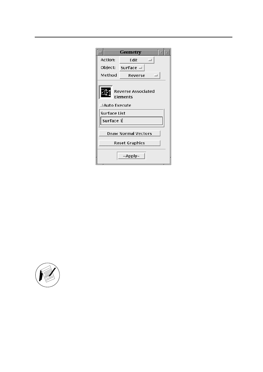
To check this change ‘Action’ from ‘Create’ to ‘Edit’. Change the ‘Object’ to ‘Surface’ and the
‘Method’ to ‘Reverse’ (see Figure 16).
Check the square button marked ‘Auto Execute’ to make sure it is unset.
Click on the box marked ‘Surface List’ and click on the Surface label 1.
21
4 CREATE GEOMETRY
4.5 Checking the Surface Normal
Figure 16: Check Surface Normal
Then Click on the box marked ‘Draw Normal Vectors’.
Now using the middle mouse button tilt the geometry (Hold down the middle mouse button
and move the mouse until you can see the direction of the normal vector clearly). The vector
starts at the centre of the surface and is directed normal to it.
If the normal vector is in the same direction as the positive Z axis then the current geometry will
create a valid finite element mesh.
If the normal vector is in the same direction as the positive Z axis
then DO NOT click on Apply.
If not then you can use the Apply button to reverse it. This can be used selectively on individual
surfaces.
Note
Note that this check only needs to be carried out for analysing 2D problems (Plane
Stress or Plane Strain). However this check is not required if using 3D solid elements
or shell elements.
First click on the box marked ‘Reset Graphics’ in this form. This will erase the
normal vector.
Repeat the above steps for surfaces 2 and 3.
As a final check draw the normal vector for all 3 surfaces. This is one of the
dialogue boxes where you don’t automatically click on APPLY. This is only done
if necessary.
Click on the ‘Front View’ icon in the toolbar. Click on the ‘Fit View’ icon if neces-
sary.
22
5 LOADS AND BOUNDARY CONDITIONS
x
z
y
Front View Icon
Spatial
Fields
Type:
Field Name
PCL Function
Create
Action:
Click in this box and
triang
enter name
Click on this to enter ‘X
in the above box.
Scalar Function
Independent Variables
Type this expression.
100 * (100 − ‘X) / 80
Object:
‘Z
‘Y
‘X
−Apply−
triang
Figure 17: Define Load Distribution Function
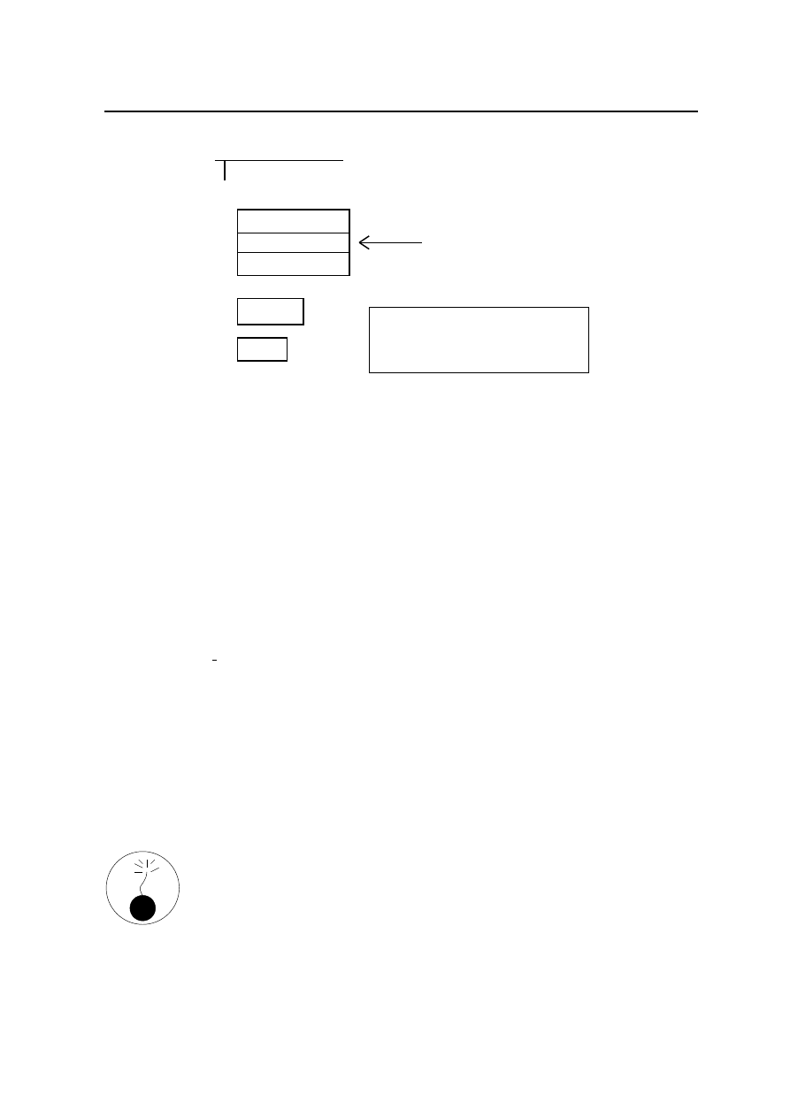
5
Loads and Boundary Conditions
5.1
Define the Load variation function
The function which defines the triangular load distribution will have to be created first before creating
the load. The loading varies as a function of the X Co-ordinate so it will have to be defined as a function
of X.
Click on the
3
Field
button which will close the Geometry form and open the Field form (see
Figure 17
).
First of all click on the box marked ‘Field Name’ and type triang (for triangular distribution).
The expression ( 100 - x ) gives a value of 80 at x = 20 and 0 at x = 100. To change this to 100 one
needs multiply this by 100 and divide by 80. The required expression is 100 * ( 100 - x ) / 80.
Click on the box marked ‘Scalar Function’ and then enter the expression as above but instead of
typing ‘X click on the ’X in the list marked ‘Independent Variables’.
Then click on the Apply button.
This completes the creation of this load function. In the history window you should see the
message :
$
# Field “triang” created.
It is possible to check this expression (see Figure 18).
23
5 LOADS AND BOUNDARY CONDITIONS
5.2 Loads and Boundary Conditions
00
00
00
00
11
11
11
11
Show
Action:
Fields
Select Field To Show
Independent Variable Range
Select this.
20.
X
2
100.
No. of Points
Maximum
Minimum
triang
−Apply−
OK
Click on this box.
Specify Range...
X
Select Independent Variable
Cancel
and the Plot Window.
To close the Dialogue Box
Click on this box.
Unpost Current XYWindow
In the Plotted Curves Form...
Figure 18: Check Load Distribution Function
Change the ‘Action’ from Create to ‘Show’. Click on triang from the list ‘Select Field to Show’.
Click on the button ‘Specify Range’.
In the new dialogue box ‘Specify page’ Enter 20 for Minimum and 100 for maximum and 2 for
the No. of Points. Then click on OK. In the original form click on APPLY.
This should display the plot of the variation in a XYWindow and also list the values in a spread-
sheet type table for the 2 points requested. This completes the check.
Click on ’Cancel’ in the ‘Plotted Curves’ form. Then click on the button marked ‘Unpost Current
XYWindow’. This should close the dialogue box and the plot window.
The next step is to create the boundary condition and the loading.
5.2
Loads and Boundary Conditions
One of the advantages of PATRAN is that one could specify the loading and boundary condition either
on the ‘geometry’ or the ‘finite element model’. If specifying the loads/boundary conditions on the
‘geometry’ it can be carried out even before the finite element mesh is generated. When this is done
the loads and boundary conditions are automatically translated to the ‘finite element model’ when it
is generated.
However in some analyses loads and boundary conditions may have to be specified directly on the
finite element mesh itself. Example : application of a point load at a node in the interior of the mesh
where there is no geometric point. This load can be specified once the finite element mesh has been
generated. The choice of applying Loads/BCs either to the geometry or the finite element mesh is
controlled by a
3
button in the ‘Select Application Region...’ form (called from
3
Loads/BCs form).
Click on the
3
Loads/BCs
button which will close the Fields form and open the Loads/BCs form
(see Figure 19).
24
5 LOADS AND BOUNDARY CONDITIONS
5.2 Loads and Boundary Conditions
B
A
fixed
New set Name
Nodal
Input Data ...
Click in this box and
DO NOT press
Action:
Object:
Displacement
Create
Select this box
< >
Translations <T1,T2,T3>
OK
enter name ’fixed’.
< 0 0 >
Click on the "curve" icon to select it. It is the 3rd icon in the select menu.
Click in this box and enter 2 zeroes
separated by spaces between
Type:
eithe geometry or the finite element
Select menu
Pick
Then click on line A. The label ‘surface 1.1’ should
Click on this and the information should
appear the ‘Application Region’.
Key
−Apply−
Select Application Region...
This selection filters screen picking. In this case only the lines will be
Rotations <R1,R2,R3>
OK
the angled brackets.
Geometry
FEM
model. The default pick is "Geometry".
The Loads and BCs can be associated with
Select Geometry Entities
Click in this box.
Add
appear in the box marked ‘select Geometry Entities’.
Leave this unchanged.
selected, although there may be surfaces or points in the area.
the RETURN key.
Load/Boundary Conditions
Repeat this by selecting line B (label Surface 2.1) .
Figure 19: Load/BC Form
25

5 LOADS AND BOUNDARY CONDITIONS
5.2 Loads and Boundary Conditions
Using this form the displacement fixity along the left hand side vertical boundary is specified.
Leave the default option of Create/Displacement/Nodal for Action/Object/Type.
First of all click on the box marked ‘New Set Name’ and type fixed .
This is the set name given to the fixity boundary condition about to be specified. Each load and
boundary conditions has to be given a set name. The user is free to choose a meaningful name
for the set.
This needs two subforms to be filled. In the first of these you specify the type of fixity. The second
subform is for selecting the region to which the boundary condition is applied. To execute the
command you need to click on the Apply button in the original form.
Now click on the box marked ‘Input Data...’.
This will open a new form.
Click on the box under the heading ‘Translations’ and enter 2 zeroes separated by spaces between
the angled brackets (
<
0 0
>
).
This is to indicate zero displacements in the 2 directions (x and y).
Leave the rest of the data in the default setting.
Click on the OK button. Then in the original form click on the ‘Select Application Region...’.
This is to specify which part of the boundary is to be fixed. Notice the
3
Geometry which is
selected.
Click on the box marked ‘Select Geometry Entities’. Now choose the ‘curve’ icon (3rd icon) from
the select menu next to the form.
This selection filters the picking. In this case only lines will be selected. Surfaces and points will
be ignored when you cursor pick entities.
As you move the mouse around you will notice that the various curves getting highlighted and
changing colour. PATRAN is indicating what is the current selection and highlighting entities
which are likely to be selected. This should help in informing you what is the current icon
selection.
Now click on the left hand side vertical line A.
This line should change colour to indicate that it has been selected.
The label of the line should also appear in the box marked ‘Select Geometry Entities’. However
if this does not happen then check the ‘Select Menu’ to see that the ‘curve’ icon is chosen.
Click on the ‘Add’ button. The label should appear in the box marked ‘Application Region’.
Now click on line B and again click on the ‘Add’ button.
If you had not made any mistakes then click on the OK button to close that form.
If by mistake you had selected a different line, then use the ‘Remove’ button on that form to
remove it from the list. Click on the line which was wrongly selected. Then check the label in the
box marked ‘Select Geometry Entities’ and click on the ‘Remove’ button. This should remove it
from the ‘Application Region’ list.
In the original form click on the Apply button.
Blue cones indicate the restraints applied to the left hand side boundary. There should be 2 sets
of cones at each location. The numbers 1 and 2 indicate which directions are restrained. The tip and
orientation of the cone indicates which direction the edge is restrained. If the tip is pointing in the
horizontal direction then that line is restrained in the horizontal direction.
If the blue cones are not displayed then you must have made a mistake. Change the ‘Action’ from
‘Create’ to ‘Modify’. Check the ‘Input Data’ and ‘Application Region’. Make sure that the correct icon
was chosen from the ‘Select Menu’. You can also change the ‘Action’ to ‘Show Tabular’ to check the
input data.
26

6 DEFINE ELEMENT PROPERTIES
5.3 Load Application
5.3
Load Application
Along the top, the side on the right hand is to be subjected to a vertical triangular distributed load
which varies from 100
N
=mm
2
to 0.
The load distribution function has already been specified in the previous section.
To specify this, set the ’Action’ to ’Create’ and change the ‘Object’ to ‘Pressure’. Enter dstld (short
for distributed loading) in the box marked ‘New Set Name’.
This is the label by which the load will be identified (Figure 20).
Click on the ‘Input Data...’ button and click on the box marked ‘Edge pressure (2-D Solids)’ and
click on the label triang in the field box marked ‘Field’. The label f:triang should be displayed in
that box.
Click on the OK button.
Then click on ‘Select Applications Region...’. Click on the box marked ‘Select Geometry Entities’.
Choose the ‘Curve’ icon from the ‘Select Menu’ (it is the 1st icon). Then click on curve marked C
in Figure 20.
The label ‘Surface 3.2’ should appear in the box marked ‘Select Geometry Entities’.
Click on the ‘Add’ button. The label ‘Surface 3.2’ should appear in the box marked ‘Application
Region’. Then click on the OK button to close that form.
In the original form click on the Apply button.
This completes the specification of the load. The load vector should be displayed in Red. The
values 100 and 0 should be displayed at either end. If this does not happen then you must have made
a mistake. Change the ‘Action’ from ‘Create’ to ‘Modify’. Check that the ‘Input Data’ and ‘Application
Region’ are correct for the above load application. You can also change the ‘Action’ to ‘Show Tabular’
to check the input data. Then proceed with the exercise.
The next step is to input the material properties.
6
Define Element Properties
First a material called steel is created and the properties defined (E,
). Then these properties are
assigned to the bracket and the thickness is also specified. These are defined in two different forms.
6.1
Define Material Properties
The bracket is made out of steel. Here it is assumed to be isotropic and linear elastic.
Click on the
3
Materials
for specifying the material properties.
Figure 21
shows the form which is used to input the material properties for the bracket.
Click on ‘Isotropic’ and look at the other constitutive models that can be chosen. Leave it un-
changed for the present.
Enter the Material Name Steel.
Select ‘Input Properties...’. Enter an Elastic Modulus of ‘2.1E5’ (in MPa), Poisson’s ratio of 0.3.
Click on the ‘OK’ in this form and then click on ‘Apply’ in the original form. This completes the
input of material properties.
If you need to check the material properties at a later stage, change the ‘Action’ from ‘Create’ to
‘Show’. To make any changes, change the ‘Action’ to ‘Modify’.
27
6 DEFINE ELEMENT PROPERTIES
6.1 Define Material Properties
C
FEM
OK
Click in this box and
Click in this box.
The Loads and BCs can be associated with either
The default pick is "Geometry".
triang
Geometry
the geometry or the finite element model.
Add
Target Element Type :
Edge Pressure (2D−Solids)
Change this from 3D to 2D.
Select Surfaces or Edges
triang in the ‘Spatial Fileds’ Box below.
This should then display ‘F : triang’.
Click in this box and then click on
Key
Select menu
Then click on top line in surface 3 (Line C in above). The label ‘Surface 3.2’
should appear in the box marked ‘Select Surfaces or Edges’.
Click on the "Curve" icon to select it. It is the 1st icon in the select menu.
This selection filters screen picking. In this case only the curves or edges
Click on this box.
Click on this and the information should
appear the ‘Application Region’.
f: triang
Spatial Fields
enter name ’dstld’.
dstld
Pressure
Type:
OK
−Apply−
Select Application Region...
Load/Boundary Conditions
DO NOT press
the RETURN key.
Input Data ...
2D
Pick
New set Name
Element Uniform
Create
Action:
Object:
will be selected, although there may be points or surfaces in the area.
Figure 20: Load Application
28
6 DEFINE ELEMENT PROPERTIES
6.2 Element Properties
Input a name and select input
Input Properties...
Material Name
Create
Isotropic
Manual Input
Materials
Action:
Object:
Method:
Properties.
Constitutive Model
Leave
unchanged.
Input these.
Leave these unchanged
Elastic
0.3
2.1E5
Steel
Poisson’s Ratio =
Elastic Modulus =
−Apply−
OK
Figure 21: Material Properties
6.2
Element Properties
Click on the
3
Properties
to assign the previously specified material properties to the geometry
and to specify the thickness of the bracket.
The form for carrying out this is shown in Figure 22.
Change the ‘Type’ to ‘2D Solid’ instead of ‘Shell’. Type ‘bracket’ in the Property Set Name box.
Change ‘Plane Strain’ to ‘Plane Stress’ under Options.
Click on the ‘Standard formulation to look at the other options. But leave it unchanged for the
present.
Click on the ‘Input Properties...’ label. In the new form click on the ‘Material Name’ box and
select ‘steel’ from the Material Property Sets. This should display ‘m:steel’ in the box marked
‘Material Name’. Enter a value of 75 in the thickness box. Click on the OK button.
In the original form click on the ‘Select Members’ box. Then choose the ‘surface or face’ icon
from the select menu (this is the first icon).
To select all three surfaces drawn a box around the whole bracket.
This would have changed the colour of all three surfaces to red. This is an alternative way of
selecting points, curves and surfaces.
The surface will change colour to orange and ‘Surface 1:3’ should appear in the box marked
‘Select Members’. If this does not happen then check that the icon selected from the ‘Select
Menu’ is the first one.
Now click on the ‘Add’ button and the list will now be displayed in the ‘Application Region’
box. Finally click on the ‘Apply’ button.
29
6 DEFINE ELEMENT PROPERTIES
6.2 Element Properties
Property Set Name
2D Solid
Dimension :
Type :
Option(s)
Properties
Plane Stress
Input Properties...
bracket
Action:
2D
Material Name
Click in this box.
Material Property Sets
"Surface 1:3" should appear in the
−Apply−
[ Thickness ]
Select ’Surface’ from the menu of icons (this is the 1st icon).
Quad 4s are 2D elements
Change this to ‘2D Solid’.
Input a name.
Change this from Plane Strain to Plane Stress.
Click on this.
Add
OK
Steel
Select our material in the
listbox that appears in the
form.
Input thickness.
Select Members
Click in this box.
Application Region box.
75
Create
Draw a box around all 3 surfaces.
Figure 22: Element Properties
30
7 FINITE ELEMENT MESH
Click here and enter the Group Name.
New Group Name
Make Current
Add Entity Selection
These are the defaults. The current group
is the one which receives all new entities.
Create ...
Group
fem
Cancel
−Apply−
Figure 23: Define a new group
The message
$
# Property set “bracket” created should appear in the history window.
When the finite element mesh is created later all the elements in the mesh would be assigned the
‘steel’ material properties.
If you need to check the properties at a later stage, change the ‘Action’ from ‘Create’ to ‘Show’. To
make any changes, change the ‘Action’ to ‘Modify’.
Note
As mentioned earlier it is possible to assign the properties either to the “geometry”
or to the “finite element mesh”. Here it has been assigned to the geometry.
7
Finite Element Mesh
Before generating the finite element mesh it is necessary to create a separate group. This
is to keep the Geometry model separate from Finite Element Model. This makes it eas-
ier to select and display the Geometry model separately from the Finite Element Model.
Groups
are like ‘named components’. Each group has its own name and contains en-
tities
. If you look at the top of the viewport you will notice the name default group
displayed. That is the default name and the created geometry is part of that group. Let us leave
‘geometry’ in the default group.
A new group called fem will be created for the finite element model.
Click on the Group label at the top window (Figure 23). Choose the Create... option. Enter ‘fem’
in the box with the heading ‘New Group Name’.
Click on the Apply and Cancel buttons respectively.
You will notice that the group name in the viewport title bar has changed from “default group” to
“fem”. This is the current group (and only one group can be the current group), and it will receive
all new entities that are to be created; i.e. the finite element mesh, nodes and elements. However the
“default group” is still posted. Here posted means ‘on display’.
7.1
Create Mesh Seeds
Mesh seeds tell PATRAN how the mesh is to be generated. The mesh is to be created with 2 elements
along the shorter sides and 8 elements along the longer sides.
Click on the
3
Elements
label which will close the Loads/BC form and open the Finite Elements
form.
31
7 FINITE ELEMENT MESH
7.1 Create Mesh Seeds
A
D
B
E
C
Auto Execute
Click on the line D (curve 1) and then click on the
Click in this box
Curve List
Then click on line C.
lines B and E (surface 2.1 & 2.2) respectively.
8
Number =
Click in this box and then click on line A.
Display Existing Seeds
2
Number =
Curve List
Key
Finite Elements
Uniform
Mesh Seed
Object:
Action:
Create
Type:
Finite Elements
Finite Elements
Finite Elements
Change this to 8.
Figure 24: Mesh Seeds
Leave the current setting of Action/Object/Type as Create/Mesh Seed/Uniform (Figure 24). The
choice of ‘Uniform’ for ‘Type’ means that the generated elements will be of equal width. It is possible
to generate a graded mesh by changing the ‘Type’ to ‘One Way Bias’ or ‘Two Way Bias’. However this
will not be attempted for this example.
The idea is to create a mesh with 8 noded quadrilateral elements.
Change the entry in ‘Number’ box to 2. Click on the ‘Curve list’.
Now click on the lines marked B, D and E respectively (shown in Figure 24).
The mesh seeds showing how the sides will be divided should appear in the lines.
Change the entry in ‘Number’ box to 8.
Click on the ‘Curve List’ again and click on the left hand vertical line (Surface 1.1, marked A
in Figure 24). Notice the internal numbering (surface 1 side 1). Where curves were not directly
created (as for curves 1 and 2) the internal numbering of entities will be used. Don’t be misled
by the reference to ‘Surface’ when you expect ‘Curve’ to appear.
Click on line marked C.
Yellow circles will be displayed along these lines. These are the ‘Mesh Seeds’. This shows where
the nodes will be created and the division of the elements.
You can use the ‘Display Existing Seeds’ option in this form to check what the current seeding is
at a later time.
It is sufficient to assign mesh seeds to 2 adjacent sides of any surface. Opposite sides of a surface
are meshed identically.
32
7 FINITE ELEMENT MESH
7.2 Create the Mesh
Mesher :
Quad
Elem Shape :
Type:
Topology :
Quad8
IsoMesh
The label ‘Surface 1:3’ should appear.
click on the Surface labels 1, 2 and 3.
Click in this box. Then HOLD the SHIFT key
Surface List
Value
0.1
Automatic Calculate
Global Edge Length
Create
−Apply−
Surface
Mesh
Finite Elements
Object:
Action:
Change this to Quad8
Figure 25: Create Mesh
7.2
Create the Mesh
Change Action/Object/method to Create/Mesh/Surface (Figure 25). Click on the ‘Quad 4’ set-
ting for ‘Topology’ and look through the available element types. For the present example choose
the Quad8 elements. This is the 8-noded quadrilateral element.
Now click on the box marked ‘Surface List’ and then hold the SHIFT key and click in the interior
of the surface or on the label of the 3 Surfaces respectively. Alternately one could have drawn a
box around the 3 surfaces.
The label ‘Surface 1:3’ should appear in the box marked ‘Surface List’.
Then click on the Apply button.
The mesh should now be generated and displayed. White lines indicate the element boundary. The
numbers in white are the element numbers and the ones in red are the node numbers. There should
be 36 elements and 159 nodes in the mesh.
It is sufficient to specify the mesh seed for adjacent lines of a surface. The opposite sides in a
surface are meshed identically. However if you had left both of a parallel set of sides unseeded then
the program uses the Global length parameter (which has a value of 12.8) as the size of the elements
to be generated along that side. If this is the case then click on the ‘undo’ icon and then click on the
‘refresh’ icon. This should delete the finite element mesh. Then change ‘Mesh’ for ‘Object’ to ‘Mesh
Seed’ and specify the mesh seeds for the sides correctly. Then re-create the mesh.
7.3
Unpost the Geometry
Now that the finite element model has been generated we can dispense with the geometry model ie
remove it from the view/display. If we had not created the group fem just before the f.e. mesh was
created then this would not have been possible. Then geometric entities (points, curves, surfaces)
would be in the same group (default group) as the f.e. entities (elements and nodes).
33
7 FINITE ELEMENT MESH
7.4 Equivalence and Optimize
Note that the Loads/BCs go away too,
Group
Post...
default_group
Apply
Cancel
fem
of posted groups.
to select it from the list
Click on "fem"
because they are in the default_group
with the geometry.
Select Groups to Post
Figure 26: Select Finite Element Model for viewing
If you had forgotten to create the fem group then no harm is done. Follow the next 3 steps.
Otherwise skip these 3 steps.
Click on the Group label at the top window (Figure 26). Choose the Create... option. Enter ‘fem’
in the box with the heading ‘New Group Name’.
Click on ‘Add Entity selection and change it to ‘All F E Entities’. Note that this step is different
from the previous instruction in creating a new group.
Click on the Apply and Cancel buttons respectively.
Now to post only the fem group.
Now change the Create... to Post.... In the new style dialogue box look at the box marked Select
Groups to Post
.
Both default group and fem are highlighted (are displayed in reverse video) to indicate that both
are currently selected (Figure 26).
Click on the ‘fem’ to select it. Now only the ‘fem’ should appear highlighted. Then click on the
Apply
button and then the Cancel button to close that form.
This should only display the finite element mesh. Click on ‘refresh graphics’ to redraw the mesh.
7.4
Equivalence and Optimize
The next two steps are Equivalence and Optimize. If you click on the ‘Create’ label in the ‘Finite
Element’ form it will display these options.
Warning
First of all look at the node numbers. If these are not on display switch these ON.
You will notice that the nodes along the shared sides of the surfaces have two sets of
numbers superimposed. These are duplicate nodes.
When PATRAN creates the mesh elements and nodes are created separately on each
surface. As a result there are 2 sets of Nodes along shared edges for 2D problems.
The ‘Equivalence’ command gets rid of the duplicate nodes. If the Equivalence
command is not used then the created f.e. mesh will have unconnected parts ie it will
be fragmented.
If the structure consists of more than one surface use of ‘Equivalence’ is mandatory.
Otherwise you will end up with a mesh which is not connected up. Here the TOLERANCE is used
to determine the duplicate nodes. Any 2 nodes situated within a distance of the TOLERANCE are
34
8 CHECK LOAD/BCS
Action:
Object:
Method:
Equivalence
Tolerance Cube
All
Nodes to be excluded
Equivalencing Tolerance
0.05
Click on this.
leave all the default
−Apply−
settings unchanged.
Figure 27: Equivalence the Nodes
considered to be duplicates. Hence the importance of making sure that the largest dimension on which
the tolerance is based on is specified reasonably accurately at the beginning
Click on Create and change it to Equivalence. See Figure 27.
Then click on the Apply .
Notice the Magenta circles which indicate where PATRAN found and deleted the duplicate nodes. In
the message window there should be a message saying that 10 duplicate nodes were deleted.
Notice the node numbers along shared sides. There should now be a unique set to node numbers
clearly readable.
The next step is to ‘Optimize’ the mesh. These would make the solution efficient. With large
number of nodes/elements optimising is recommended.
Click on Equivalence and change it to Optimize.
Change the ‘Method’ to ‘Both’. Click on the ‘Apply’ button.
A table will be displayed with the details of optimisation.
Click on the ‘OK’ button in that form.
8
Check Load/BCs and Create a Load Case
The next step is to create a load case which combines the selected load and boundary conditions into
a single set. But first, we will demonstrate displaying the Loads/BCs on the FEM model.
This is done in two steps. The first is to set the display mode. The second is to replot the markers
from Loads/BCs to cause them to be evaluated on the FEM model.
35
8 CHECK LOAD/BCS
8.1 Loads/BCs
Display
Press this to switch it on.
Cancel
Load / BC / Elem.Props ...
Show All
Show on FEM only
Show LBC / El. Prop. Vectors
Press this to switch it on.
Notice that there is no visual
appearance change. You’re just
changing a switch setting.
Apply
Figure 28: Switch Display On
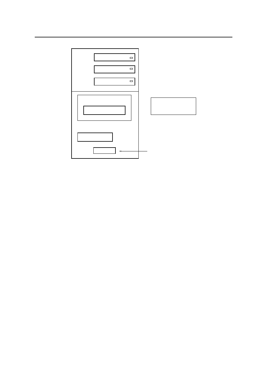
Loads/BCs
Action :
Plot Markers
Assigned Loads/BC Sets
Select Groups
Displ_fixed
Press_dstld
Click on the names of the sets we
just created to select them. Hold down
the shift key when selecting the 2nd item.
The 5 letter prefixes remind you
fem
Click on the name of the group
containing our elements.
Verify that the displacement
markers are at the nodal points.
−Apply−
of the set type.
Figure 29: Plot Markers
8.1
Loads/BCs
Figure 28
shows how to switch the display on.
Click on ‘Display’ and choose ‘Load/BC/Elem. Props...’. In the new form click on the button
marked ‘Show All’ below the box marked Loads/BCs.
Make sure that the button marked ‘Show on FEM only’ is ON; i.e. in the pressed down position.
Click on the ‘Apply’ and ‘Cancel’ buttons respectively.
There will not be any visible change at this point.
Choose
3
Loads/BCs
. Choose the ‘Action’ Plot Markers (Figure 29). Click on the name of the
set Displ fixed to select it, from the box marked ‘Assigned Load/BC Sets’. Then hold down the
shift
key and click on the name of the set Press dstld to select it as well. From the ‘Select Groups’
select ‘fem’. Then click on the ‘Apply’ button.
This will display the displacement markers at the nodes and the load vectors for each element
side. If either or both of the markers are missing then check that you have selected both sets
(fixed, dstld).
36

9 PERFORM THE ANALYSIS
8.2 Create a Load Case
Display
Let’s remove the markers
from the display.
Load / BC / Elem. Props ...
Hide All
Press this to switch it OFF.
Apply
Cancel
After clicking on this click on the
Reset graphics icon to clear the markers.
Show on FEM only
Figure 30: Switch Display Off
Now that the displacement fixities and loads have been verified for the f.e.mesh the display can
be turned off as follows (Figure 30) :
Click on ‘Display’ and choose ‘Load/BC/Elem Props...’. In the new form click on the button
marked ‘Hide All’ below the box marked Loads/BCs. Also unset the toggle ‘Show on FEM
Only’. Click on the ‘Apply’ and ‘Cancel’ buttons respectively.
You can use the ‘refresh’ icon to re-draw the mesh, in case part of the mesh got erased due to the
last command. The next step is to create a load case with the loading and boundary conditions.
8.2
Create a Load Case
A load case combines user selected load and boundary conditions. Next step is to create a load case to
combine the boundary condition, ‘fixed’ and the loading ‘dstld’.
Choose the
3
Load cases
. In the box marked ‘Load Case Name’ enter ‘dist load’. Then click
on the Assign/Prioritize Loads/BCs. This will bring up a new form (Figure 31). From ‘Select
Individual Loads/BCs’ select Disp fixed and Press dstld.
If any one of the items makes more than one appearance (by accidentally clicking more than
once) then ensure that the scale factor is 1.
If more than one appearance is made then
select the row (by clicking on any cell in that row) and then click on button marked Remove All
Rows
and repeat the step.
Click on the ‘OK’ button and then click on the ‘Apply’ button in the original form.
This completes the data input. The message Load Case “dist load” created should appear in the
history window.
9
Perform the Analysis
9.1
Submit a ABAQUS Analysis
We’re ready to analyse the problem we’ve entered in PATRAN.
Click on the
3
Analysis
label.
Figure 32
shows the form.
37

9 PERFORM THE ANALYSIS
9.1 Submit a ABAQUS Analysis
Pressure
Displacement
dstld
Assigned Loads/BCs
Remove All Rows
Remove Selected Rows
Add
1.
Add
Scale factor
Type
Priority
1.
fixed
−Apply−
Assign/Prioritize Loads/BCs
Displ_fixed
Select Individual Loads/BCs
Click on this box and
enter name.
Click on this box.
Use these if you make
any mistakes.
should appear in the spreadsheet below.
created to select them. Then these
Click on the names of the sets we just
Press_dstld
dist_load
Load Cases
Load Case Name
OK
Figure 31: Create a Load case
Click on ‘Step Creation...’ and in the new form enter in the box marked ‘Job Step Name’ :
static loading
.
Notice the default option of Linear Static for the ‘Solution Type’.
In the box marked ‘Job Step Description’ enter ‘Static analysis with pressure loading’.
Click on the ‘Linear Static’ and this will display other type of analyses that can be carried out.
For the present leave this as ‘Linear Static’.
Click on the box marked ‘Select Load Cases...’ and in the new form select the ‘dist load’ from the
available load cases. Then click on the ‘OK’ button to close that form.
Click on the label ‘Output Requests...’ and check the default options for future reference. Change
the ‘None’ for ‘Stress Invariants’ to ‘Integ Point’. Then click on the ‘OK’ button to effect the
changes made.
Click on the ‘Apply’ and ‘Cancel’ buttons respectively in the ‘Step Create’ form. This will close
that form.
Click on the ‘Step Selection...’ button in the original form. Click on the ‘static loading’ in the
‘Existing Job Steps’ box and this will appear in the box marked ‘Selected Job Steps’. Then click
on ‘Apply’.
Now all the data input is complete.
Finally click on the ‘Apply’ button to submit a ABAQUS job.
PATRAN creates the input data file called bracket.inp (for this example) and submits a ABAQUS
job. The abaqus job is run external to the patran session. The following messages should appear in the
history window :
1. Executing /export/../patran2003r2/bin/pat3aba.
38
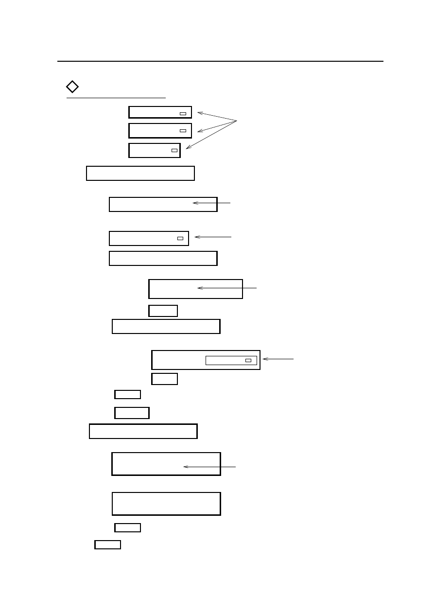
9 PERFORM THE ANALYSIS
9.1 Submit a ABAQUS Analysis
Existing Job Steps
Selected Job Steps
Default Static Step
static_loading
Click on this to add it to the
Selected Job Steps.
static_loading
Method:
static_loading
Job Step Name
Click in this box and enter name
Solution Type
Click on this for other
type of analysis.
Full Run
Object:
Entire Model
Analyze
Action:
Leave these unchanged
Analysis
Available Load Cases
Click on this name to select it.
Stress Invariants
Integ Point
Step Creation...
Select Load Cases...
OK
The default is
None.
If we don’t turn these to
Cancel
Step Selection ...
Apply
Apply
Apply
plot will be unexciting.
Integ Point the results
OK
Output Requests...
Output Variables
Option
dst_load
Linear Static
Figure 32: Run an ABAQUS Analysis
39

9 PERFORM THE ANALYSIS
9.2 Accessing the ABAQUS Results from PATRAN
2. translator messages may be found in the file ./bracket.msg.01.
3. Executing /export/../patran2003r2/bin/AbaqusExecute.
First the viewport will be closed and the Message Generating Input for ABAQUS would appear
in a separate window which would be closed subsequently. At this point he ABAQUS job starts to run
(in the background). The viewport should be back on display.
Now move the viewport aside and look in the xterm window from which patran was started. Look
for the message : Sending output to nohup.out in that window. In the absence of any other message
this would in general mean that the analysis was successful. However in case of errors the following
message may appear in the same window.Error detected ... Aborting AbaqusExecute. In case of
errors you must find the errors and correct them. First look in the file called nohup.out. It might
suggest looking at either bracket.msg or bracket.dat file.
Notice the difference between the files bracket.msg.n and bracket.msg. The bracket.msg file is
created by ABAQUS and is a report of the analysis whereas bracket.msg.n is a report from PATRAN
in creating the ABAQUS input file (whether creation of each keyword was successful or not).
The following steps are involved. First the ABAQUS input file is written to. The report of this
action is written to a file bracket.msg.01 when it is the first time. If the file(s) bracket.msg.n already
exists then a new file with the last 2 digits incremented by 1 will be created. Look for the file with the
largest extension number. The next step in the absence of any errors in the input creation step is to run
the ABAQUS analysis.
Then wait for the abaqus job to finish. Type top in the second X-term window and wait till ‘pre.x’
and ‘standard.x’ disappear from the displayed list. Because this is such a small example you will have
to be quick to see this. Type q to quit from top.
The files bracket.dat and bracket.odb would have then been created. If either or both these files
are missing then there could be an error in the data input. Check the file bracket.msg.01 for error
messages. Check also the bracket.inp file.
If both these files (*.dat and *.odb) are successfully created then resume the PATRAN session as
described in the next section.
This list summarises the general suggestions on what to do after the analysis is complete.
Use one of the other xterm. Make sure that the current directory is patran.
more nohup.out Read the ABAQUS log file.
more bracket.inp View contents of ABAQUS input file.
more bracket.msg View message file.
emacs bracket.dat View ABAQUS output file using emacs.
Use File / Exit Emacs to quit from Emacs.
rm nohup.out Remove this file. It will be recreated.
9.2
Accessing the ABAQUS Results from PATRAN
The ABAQUS printed results will be written to bracket.dat (ascii). The output database is called
bracket.odb (binary). In order to access the results from PATRAN you need to attach the ‘*.odb’ file to
PATRAN.
Click on the
3
Analysis
form to re-open it.
Change the ‘Action’ from ‘Analyze’ to ‘Read Results’.
The form is shown in Figure 33.
40
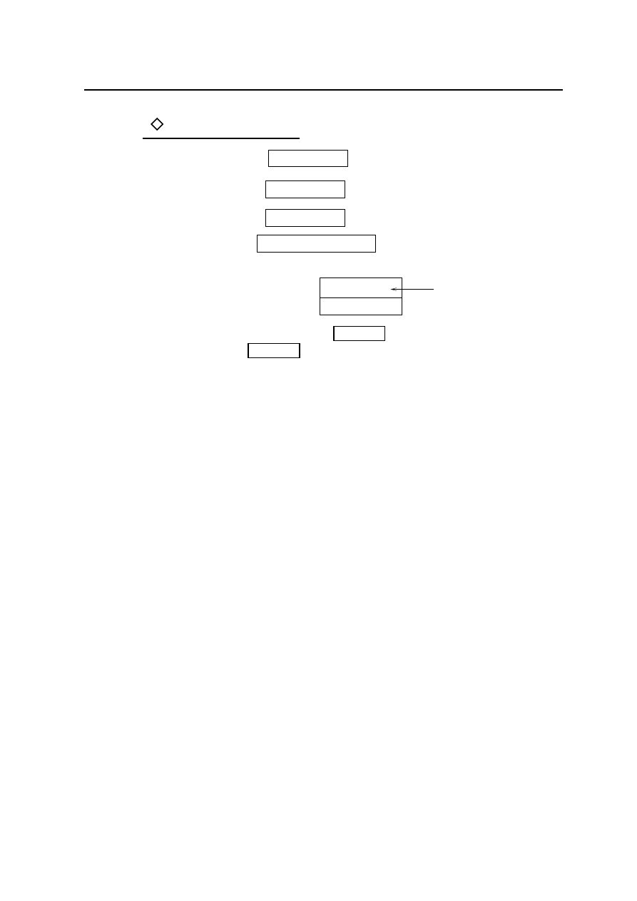
9 PERFORM THE ANALYSIS
9.2 Accessing the ABAQUS Results from PATRAN
Analysis
Action :
Object :
Method :
Attach
Results Entities
Read Results
Available Files
Select this file
Select Results File...
Apply
OK
bracket.odb
Figure 33: Attach to the ABAQUS Output Database
Click on the label ‘Select Results File...’.
This will bring a new form up. Check under the heading ‘Available Files’. If ‘bracket.odb’ does
not appear in the list then the ABAQUS job has not run so far or there may have been some
errors.
Wait for a while and click on the ‘filter’ button to update the list of available files.
It is good practice to check the contents of the file ‘nohup.out’ to see whether the run was suc-
cessful.
Check the date and time because the contents of the file ‘nohup.out’ are cumulative and the
outcome of the current run is appended to the existing file. Also it is a good idea at this point to
delete the file ‘nohup.out’ as it will be re-created.
rm nohup.out.
Now proceed with the post processing.
If the file ‘bracket.odb’ is present then select it by clicking on it.
This file name should then be displayed in the box marked ‘Selected Results File’.
If the file ‘bracket.odb’ is not present then either the job was not run or there may have been errors
in the input data. Use the second window to see whether the file ‘bracket.dat’ and ‘bracket.msg’
are present. If present then look through these files for a possible explanation. You need to take
remedial action before you can carry on with the exercise.
If there are no errors then
Click on the OK button. Click on the ‘Apply’ button in the original form.
There will be messages of progress in the history window. The heartbeat will turn red and then
to blue as the results are set up for direct access from the database. Wait till it turns green again. The
viewport may be cleared and the mesh may be redrawn meanwhile.
The following message should appear in the history window :
41

9 PERFORM THE ANALYSIS
9.3 Post Processing
$# Attaching Direct Results Access file:
$# "/amd_tmp/needle-16/usersn/.../patran/bracket.odb"
$# Creating Group "PART-1-1".
$# Creating Group "FEM".
$# Creating Group "FIXED".
$# Creating Group "BRACKET".
$# Attaching Direct Results Access file:
$# "/amd_tmp/needle-16/users0/.../patran/bracket.odb"
$# *** Begin: Attach MSC.Patran Access
Result File ***
$# Processing result load case: Step-1
$# Processing result sub-case: Frame 0, Time 0
$# Processing result sub-case: Frame 1, Time 2.22e-16
$# Total execution time in real seconds:
0.000
$# Total execution time in CPU
seconds:
0.140
$# *** End: Attach MSC.Patran Access
Result File ***
In case of any problems with post-processing look at this file in a separate X-term window.
$# Error reported from application Results
$#
Direct Results Access file is already attached. To re-attach with
$# different Translation Parameters, please detach the file using the
$# Analysis form option Delete "Attachment" then re-attach. File:
$# "/amd_tmp/needle-16/usersn/.../patran/lp2.odb"
$? NO 4012005
$# Question from application Results
$#
Detach from Direct Results Access file:
$# "/amd_tmp/needle-16/usersn/.../patran/lp2.odb". This operation
$# cannot be undone. Do you want to continue?
$? YES 4012012
$# Detach external results file:
$# /amd_tmp/needle-16/usersn/.../patran/lp2.odb
This above listing is purely for illustrative purposes. It shows a different analysis where errors
were encountered. In case of similar errors you need to find the source of the errors. Then after
making corrections if you want to re-run ABAQUS using the same job name then you need to delete
the Result attachment of the the ‘*.odb’ file to PATRAN first. This is done as follows :
In the
3
Analysis
form,
Change the ‘Action’ to ‘Delete’ and the ‘Object’ to ‘Result Attachment’.
Select the ‘bracket.odb’ and then click on ‘Apply’.
Now the bracket.odb file is detached. Run the ABAQUS analysis again and then re-attach the
results file. Then proceed to the next section.
9.3
Post Processing
Choose the
3
Results
option.
Figure 34
shows the form.
Change the ‘Object’ from Quick Plot to Deformation. ‘point load’ should be highlighted in
‘Select Result Cases’.
42
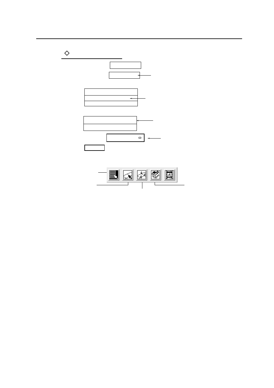
9 PERFORM THE ANALYSIS
9.4 Changing Display Parameters
Object :
Select Deformation Result
Step 1, ... Frame 1
Step 1,... Frame 0
Select Result Cases
Results
Deformation
Click on ‘Quick Plot’ and change it to
‘Deformation’.
Click on the result case name.
Deformation, Displacement
Select Displacements.
Show As :
Resultant
Create
Action :
Apply
Leave unchanged
Figure 34: Results Form
Select Results
Plot Options
Target Entities
Display Attributes
Icons in the Results Form
In the ‘Select Deformation Result’ listbox select ‘Deformations, Displacement’. The ‘Show As’
should be set to ‘Resultant’. Click on the ‘Apply’ label.
You should see the deformed mesh plotted in white on the viewport. The blue lines represent the
undeformed mesh. Notice the value of 1.82 displayed next to the node where the load is applied. This
is the largest displacement.
9.4
Changing Display Parameters
To change the scaling used for the displacement
Click on the ‘Display Attributes’ icon. Turn the ‘Show Maximum Label’ off (Figure 35).
You will notice the value 0.1 in the box marked ‘Scale Factor’ and the radio button ‘Model Scale’
is selected. This means that the largest displacement in the mesh is scaled to be 10% of the
maximum model size.
To look at the displacements at true scale
Click on
3
True Scale
to set it and enter a factor of 1 and then click on ‘Apply’.
The displacements are very small.
Enter a scale factor of 10. (Because the maximum displacement is 1.82). Click on
3
True Scale
to
set it. Now the displacements are directly multiplied by 10. Turn off ‘Show Undeformed’.
Click on ‘Apply’ on the Results form to redraw the deformed mesh.
Now click on the Reset button in this form to restore the original setting.
43
9 PERFORM THE ANALYSIS
9.5 Hard Copy of Plot
True Scale
10.
Display
Attributes
Show Undeformed
this
will be scaled accordingly
Scale Factor
on. Displayed deformations
Click on this.
Turn this
Show Maximum Label
Enter a scale factor of 10 and turn
Apply
Turn this
model will be displayed.
off. Only the deformed
off.
Figure 35: Change Display Properties
9.5
Hard Copy of Plot
To get a hard copy of the generated plot
Click on ‘File’ and select ‘Print...’.
Make sure that ‘DPO Postscript Printer’ is highlighted in the ‘Available Printers’ box. This allows
for a postscript file to be created.
If you want to send the plot directly to the printer then
Click on Apply.
Alternatively if you want to save the plot in a file then
Click on ‘Page Setup...’. This allows for the change of paper size, margins and page orientation.
For the present do not change any of the default settings. Click on ‘Cancel’ to close that form.
Click on ‘Options...’. This gives a choice of black and white or colour output to be created. Click
on ‘Print to File’. This selects the option to create a file. Make sure ‘bracket.ps’ is displayed in
the box marked ‘Filename’. However if you require to use the output in a latex document then
click on ‘Create EPS File’. This chooses the encapsulated postscript file option. Click on the OK
button.
Click on the ‘Apply’ button in the original form. This creates the postscript/eps file. When the
plotting is complete the following message will be printed in the history window.
Postscript file [bracket.ps.01] or [bracket.eps.01] complete.
The choice of whether the plot is to be sent directly to the printer or written a file is controlled by
by the settings in the ‘Options...’ form.
If one of the
3
buttons is chosen then the plot is written to a file in postscript or eps format depend-
ing on which
3
is selected.
To send the plot directly to the printer unset both
3
options.
Click on the Cancel button of the ‘Print’ form to close it.
The file ‘bracket.ps.01’ or ‘bracket.eps.01’ would have been created. Figure 36 shows the gener-
ated plot. Every time a new postscript file is created the number represented by the last 2 digits will
automatically get incremented.
44
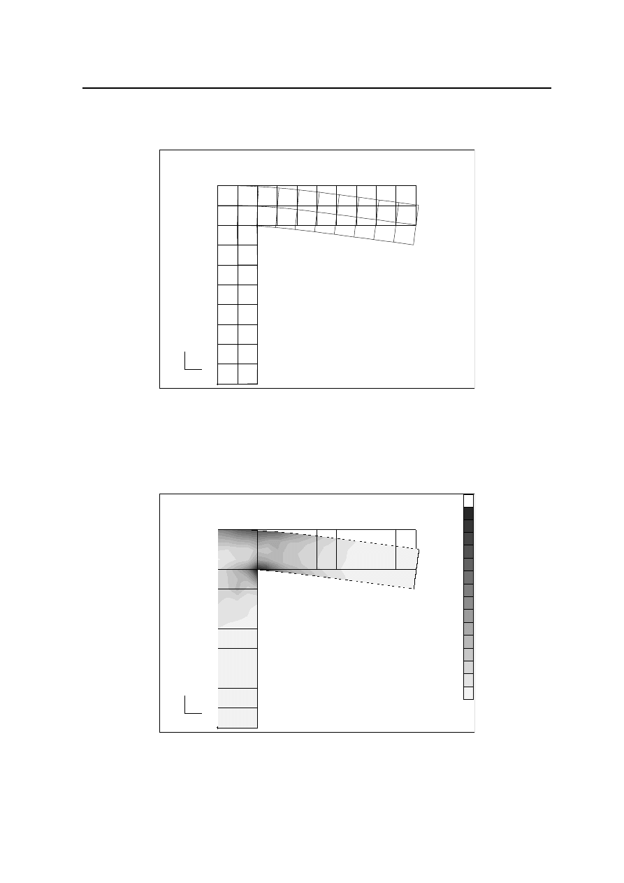
9 PERFORM THE ANALYSIS
9.5 Hard Copy of Plot
X
Y
Z
1.82+00
default_Deformation :
Max 1.82+00 @Nd 147
MSC.Patran 2003 r2 15-Oct-03 17:40:29
Deform:Step-1, A1:Frame 1, Time 2.22e-16, Spatial displacement, U, Layer 1
X
Y
Z
Figure 36: Deformed Mesh
X
Y
Z
1.79+03
3.33-01
1.79+03
1.67+03
1.55+03
1.43+03
1.31+03
1.19+03
1.07+03
9.54+02
8.34+02
7.15+02
5.96+02
4.77+02
3.58+02
2.39+02
1.19+02
3.33-01
default_Fringe :
Max 1.79+03 @Nd 81
Min 3.33-01 @Nd 8
default_Deformation :
Max 1.82+00 @Nd 147
MSC.Patran 2003 r2 15-Oct-03 17:40:55
Fringe:Step-1, A1:Frame 1, Time 2.22e-16, Stress components, S - von Mises, Layer 1
Deform:Step-1, A1:Frame 1, Time 2.22e-16, Spatial displacement, U, Layer 1
X
Y
Z
Figure 37: von Mises Stress Fringe Plot
45

9 PERFORM THE ANALYSIS
9.6 Stress Fringe Plot
9.6
Stress Fringe Plot
The next step is to produce a fringe plot of sigma-xx stress (see Figure 37). This is derived from the
general stresses. The Results menu is already selected and up.
Change the ‘Object’ from Deformation to Fringe.
Choose the ‘Stress, Components, S’ from the ‘Select Fringe Result’ table.
This will automatically select ‘von Mises’ for ‘Quantity’ which is the default choice.
Click on the Apply button.
This should display the fringes on the deformed mesh plot. This is shown in Figure 37. If you
require a fringe plot on the undeformed mesh plot then
click on the reset graphics icon to clear the previous plot and then click on the ‘Apply’ button to
redraw the fringe plot.
Click on ‘Display Attributes’ icon.
Change ‘Display’ from ‘Free Edges’ to ‘Element Edges’ and then click on the ‘Apply’ button.
To get a hard copy of the plot
Click on the ‘File’ label in the pull-down menu and choose the ‘Print...’ option.
Click on the ‘Apply’ button.
This will create a postscript file.
However if you require a colour plot then
Click on the ‘Options...’ button.
Click on the ‘Black to White’ button and change the option to ‘Color’. Click on the ‘OK’ button.
Then click on the ‘Apply’ button in the original form.
This will create a colour postscript file.
Click on the ‘Cancel’ button to close the Print form.
9.7
Using Graph (XY) Plot to plot Stress variation
The Graph (XY) Plot option can be used to produce plots of results against distance. For example to
plot the variation of the horizontal stress (Sigma-xx) along the fixed edge. Graph (XY) Plot has more
options to produce plots.
Click on ‘Fringe’ and change it to ‘Graph’ for the ‘Object’ option.
Method should display ‘Y vs X’. Y should be set to ‘Result’.
In the List box marked ‘Select Y Result’ select ‘Stress, Components’.
Change ‘Quantity’ to display ‘X Component’.
For X change ‘Coordinate’ to ‘Path Length’. Click on the ‘target entities’ icon (2nd icon) in the
Results form. In the new form the ‘Target Entity’ should be set to ‘Path’. For ‘Additional Display
Control’ change the ‘Points’ to ‘Curves’. Increase the ‘Points for Segments’ from 3 to 10.
Click on the box marked ‘Select Path Curves’ and enter surface 1.1 2.1.
Click on the ‘Display Attributes’ icon. In the new form set ‘Append Curve in XYWindow’
To save the plots that are created
46

10 FILES
9.8 To Quit from PATRAN
click on the ‘Plot Options’ icon and enter a title (Stress Sigma-xx along fixed edge) in the box
marked ‘Save Graph Plot As’.
Then click on the ‘Apply’ button.
The key here is to use the four icons displayed to set all the required settings. Only then should
the ‘Apply’ button at the bottom of the form be pressed.
You can use the options available in this form to change the appearance of the plot (to change
the line style).
Further options are available under
3
XY Plot to change the appearance of the plot (to add titles
to the axes, change grid marks, to change the plot types). Choose ‘Action : Modify’ and ‘Object :
Axis’, for example).
To get a hard copy of this
Click on File in the top menu and choose ‘Print...’.
In the form that appears change the category from ‘Current Viewport’ to ‘Current XY Window’.
Check that the ‘Available printers’ is ‘DPO Postscript Printer’. Click on the ‘Apply’ button. If
you have chosen the postscript option throughout the file will have the name bracket.ps.03. In
the command window the following message will appear
Postscript file [bracket.ps.03] complete.
Plots of other variables along the same path can be created in the same XY Window. If you
require a different type of plot then create a new XY Window with a title ‘Results Graph2’ (in the
box marked ‘XY Window Name’ in the form selected using the ‘Display Attributes’ icon).
To get rid of the previous XY Window
Click on
3
XY Plot. Choose the ‘Action : Post’ and ‘Object : XY Window’. In the box marked
‘Post/Unpost XYWindows’ click on ‘Results Graph’ by holding down the Control key and click-
ing the left mouse button. This should unselect that window. The Results Graph should now
disappear.
9.8
To Quit from PATRAN
Click on ‘File’ and choose ‘Quit’ from the menu option.
Since the contents of the PATRAN database is always up to date (when the heartbeat is Green)
the quit option closes the database and exits from PATRAN.
You can restart from here any time you wish.
This completes the exercise. By now you should have some idea of what is involved in setting up
a ABAQUS analysis, running it and post processing the results.
More examples can be found in the on-line document help page. Click on ‘Example problems’.
However these examples are for different analysis programs. Hence if you are using ABAQUS expect
some differences.
10
Files
After using the PATRAN program you will notice that the following files have been created:
1. bracket.db (database), bracket.db.jou (journal file) [Retain]
2. patran.ses.01 (session file(s)) [Retain]
3. bracket.msg.01, bracket.msg.02 (message files) [Delete]
4. bracket.ps.01, bracket.ps.02, bracket.ps.03 (postscript files) [Delete after printing]
47

11 TROUBLESHOOTING
5. bracket.inp, bracket.dat, bracket.odb, bracket.msg, bracket.sta (ABAQUS files) [Delete]
If you have taken more than one session of PATRAN to complete this exercise, there will be more
than 1 session file.
Do not delete the bracket.db.jou, patran.ses.01 files. The first is a journal file which contains all the
commands you have used in completing this exercise.
This file can be used to recreate the database (bracket.db). Therefore this file is useful if you happen
to delete the database file or if it gets corrupted.
If this happens run PATRAN and click on File and choose Utilities / Rebuild... In the new form,
select ‘bracket.db.jou’ from the list of files and click on the OK button. This will rebuild the database,
but this is a slow process and will take time.
The session files can be used to playback the whole exercise and can be useful in demonstrations.
Choose the Session / Play... under the ‘File’ command and then use the patran.ses.01 file to play back
the exercise.
lp -dljmr1 -opostscript file-name
Example : lp -dljmr1 -opostscript bracket.ps.01
The postscript files should be deleted to save disk space after these have been printed.
The ABAQUS files can also be deleted if you had used the ABAQUS option.
11
Troubleshooting
1. You are typing data into a box and it is not displayed in the box. Make sure you have clicked on
the box first to indicate that you wish to input data into that particular box.
2. PATRAN has put up an error message and when you click on the ‘OK’ button to acknowledge
it nothing happens. All the windows are ‘frozen’. Move the PATRAN windows aside to reveal
the window from which you invoked PATRAN; i.e. typed patran. On this window press the
CTRL/C keys; i.e. press the C key while holding down the CTRL key. This in general should
allow you to continue with the PATRAN session.
3. You are trying to delete some data in one of the boxes using the Delete char key and it does not
work. This could be due to some key mapping problems. Try the alternative of highlighting
the entire entry in that field/box and then use the ‘Backspace’ key to delete the current entry.
Then re-type the required entry. If this does not work then choose ‘File...’ and choose ‘Quit’ to
quit from PATRAN. Then logout and login again. Sometimes this will solve the problem. If it
does not then report it to the computer operators and give them the terminal number (example :
tw603).
4. You are trying to select an entity “Curve/Line, surface” or “Element, node” by either clicking on
the entity or drawing a box around it. But Patran does not recognise it and beeps. Usually when
Patran recognises the selection it will change the colour of the selected item and also display the
label of the selected entity.
If this does not happen then
(a) Check that the icon chosen (shown highlighted) in the ‘select menu’ is the correct one.
(b) Check that the group currently posted in the viewport is the correct one. ‘default group’
will contain the geometric entities. ‘fem’ (for this example) will contain the f.e. entities.
For example if f.e. mesh is currently posted in the viewport and in ‘select menu’ you had
chosen a geometric entity (example ‘Curve’) then this can happen. Post the ‘default group’
to select the curve. Alternatively post the ‘fem’ to select element or node.
(c) Check the form to see which radio button
3
is selected : Geometry or finite element.
5. Instruction says to click on either OK or Apply in a form but one cannot see neither of these.
This may be due the default size of the form being short. Lengthen the form window.
48

12 FREQUENTLY ASKED QUESTIONS
12
Frequently Asked Questions
See the web page under Help / Engineering Packages / finite elements / PATRAN for answers to
FAQs (Frequently Asked Questions) about PATRAN.
49
and
These terms are used interchangeably to describe
the rectangular boxes containing widgets. Each form
has a name at the top.
Same as ‘‘Do it’’. Initiates performance of all form
related actions. When it appears as ‘‘-Apply-’’ the
actions can be undone (Use Top Menu eraser icon).
Closes the form without taking any action, i.e.
‘‘cancel this order’’.
Same as Apply, but form closes (goes away) automatically.
Buttons with little rectangle present a list of selections
when pressed (called ‘‘popup’’ selections).
In general, sets all form inputs back to their values at
Really means
is automatically performed each time a selection is made
in the box immediately beneath.
Little
buttons are used for selecting choices.
Any number, from none at all, can be selected by
Appendix A : Brief Notation Review
clicking on squares.
buttons, however, are choice
the previous slelection.
Permitted Characters : A to Z, a to z, 0 to 9, underscore, hyphen, period.
Not Allowed : Spaces, parenthesis, brackets, commas, +, !, ?, =, etc.
Length :
1 to 31 characters
Forms
Menus
Solution Parameters...
Apply
Three periods
this it will bring up another form.
Cancel
OK
Label
Reset
the last time Apply was selected.
Auto Apply.
Auto Execute
square
Choice 1
Choice 2
Choice 3
Choice 1
Diamond
Choice 2
Choice 3
Only one can be selected. Clicking on another deselects
Rules for Creating Names
toggles.
Apply
’’, an
on
When ‘‘
following a name means if you choose
Here is a short summary of the notation.
A
B
making selections. To make
multiple selections, hold down the
Shift key while making them.
Use the right mouse button and
hold down the shift key to
deselect any item selected in
error.
MOUSE
Descriptive Title
Thing_1
Thing_2
Thing_3
Cursor Selecting Entities
Picking
With the cursor at point
mouse and
the cursor to point ‘‘B’’
E
B
C
D
Polygonal
Picking
mouse button at A, B, C, D and E. Choose
and select
points that surrond the entities to be selected.
You can hold down the
entities individually in sequence.
creating a selection box encompassing the entities.
Release the mouse button to initiate the selection
process. Selected entities turn orange.
Help
There are
ways to access on-line help. If you need help while filling out a
form, place your cursor on the form and press the
This accesses the user manual and brings up a copy of the form with more
information. The second method of accessing
right hand side of the Main Window.
A
left
Hold down
Shift Key
‘‘A’’, hold down
left
drag
Rectangle
two
The left mouse button is used for
the
(ctrl) and click the
Control Key
the
key on the keyboard.
F1
is to select help at the top
help
select
deselect
left mouse button
To an item or individually select additional items,
left mouse button.
To highlight a , select the top item with the
block of items
, then hold the down and use the
left mouse button
shift key
to select the last item.
left mouse button
hold down the and use the
control key
To an item, use the and highlight the item.
Listbox
This is a . It has a title at the top and a list of contents.
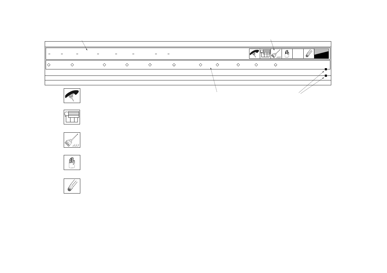
Display
Preferences
Tools
Insight Control
Viewing
Undo
Removes all fringe and marker plots, all automatic titles,
model in wireframe mode.
Interrupt
Interrupts a command in progress. This is useful when you want
to abort out of an executing PATRAN form.
Undoes the last executed action of a PATRAN form when an
highlighting and deformed shape plots. Repaints the
Brings the viewport to the ‘‘front’’ of the main form.
Refresh
beat
Heart
Help
XY Plot
Insight
Results
‘‘−Apply−’’ was pressed. (Note the dashes around Apply).
Pull−Down Menus
Application
MSC/PATRAN Version 2003 r2
move it up or down as required.
button on these markers and
Hold down the left mouse
of the Tool Bar region and
the History Window.
to change the relative size
These markers can be used
Radio Buttons
System icons
Redisplays (refreshes ) all of the graphics Viewports.
Default Window Layering
Command Line
History Window
Tool Bar Region
Analysis
Fields
Load Cases
Group
Viewport
Properties
Materials
Load/BCs
Finite Elements
Geometry
when the picture gets disturbed.
MSC
File
0 0 0 0 0
1 1 1 1 1
000 000 000 000
111 111 111 111
0 0 0 0
1 1 1 1
00 00
11 11
Reset Graphics / Display Cleanup
Wyszukiwarka
Podobne podstrony:
Game Programming Beginners Guide
Frater Jullianus Beginners Guide to Crowley
Foraging A Beginners Guide for Foraging Wild Edible Plants
Beginner's Guide To Hacking
drug ! The Beginner s Guide to Hash Growing
Kundalini Yoga Beginners Guide
Matlab Beginners Guide (ang)
eCourse A Beginners Guide to Choosing Wine
Aquarium Tropical Fish A Beginners Guide
Beginner s Guide to Growing Marijuana
beginners guide to internet riches
Crop Circles A Beginner s Guide by Hugh Manistre prev published 1999 (2002)
Wicca, A Beginners Guide to Earth Magic
Beginners Guide to Growing Marijuana
NLP for Beginners An Idiot Proof Guide to Neuro Linguistic Programming
a practical guide on pharmacovigilance for beginners
Cambridge University Press A Guide to MATLAB for Beginners and Experienced Users J5MINFIO6YPPDR6C36
więcej podobnych podstron