Detecting Malicious Network Traffic Using

Inverse Distributions of Packet Contents

Vijay Karamcheti, Davi Geiger, Zvi Kedem

Courant Institute of Mathematical Sciences

New York University

{

vijayk,geiger,kedem

}

@cs.nyu.edu

S. Muthukrishnan

Department of Computer Science

Rutgers University

[e-mail]

ABSTRACT

We study the problem of detecting malicious IP traffic in the net-
work early, by analyzing the contents of packets. Existing systems
look at packet contents as a bag of substrings and study charac-
teristics of its base distribution B where B

(i) is the frequency of

substring i.

We propose studying the inverse distribution I where I

( f ) is the

number of substrings that appear with frequency f . As we show
using a detailed case study, the inverse distribution shows the emer-
gence of malicious traffic very clearly not only in its “static” col-
lection of bumps, but also in its nascent “dynamic” state when the
phenomenon manifests itself only as a distortion of the inverse dis-
tribution envelope. We describe our probabilistic analysis of the
inverse distribution in terms of Gaussian mixtures, our preliminary
solution for discovering these bumps automatically. Finally, we
briefly discuss challenges in analyzing the inverse distribution of
IP contents and its applications.

Categories and Subject Descriptors

D.4.6 [Security and Protection]: Invasive software

General Terms

Security

Keywords

worms, inverse distribution, content analysis

1.

INTRODUCTION

To cope with increasingly sophisticated network attacks, a grow-

ing number of network security tools inspect the contents (as op-
posed to just headers) of network packets, either individually or at
the level of flows. For the most part, such inspection is restricted to
matching packet contents against a pre-established set of signature
patterns. However, researchers [8, 15, 9, 13] have recently started
advocating more general analysis of traffic contents to try and dis-
cern signals indicative of malicious network activity.

Permission to make digital or hard copies of all or part of this work for
personal or classroom use is granted without fee provided that copies are
not made or distributed for profit or commercial advantage and that copies
bear this notice and the full citation on the first page. To copy otherwise, to
republish, to post on servers or to redistribute to lists, requires prior specific
permission and/or a fee.
SIGCOMM’05 Workshops, August 22–26, 2005, Philadelphia, PA, USA.
Copyright 2005 ACM 1-59593-026-4/05/0008 ...

$

5.00.

Our work follows this trend, investigating whether statistical anal-

ysis of the contents of packets seen at one or more network ele-
ments can be used to detect the onset of a network-wide computer
worm attack. Our approach complements perimeter defenses such
as portscan detectors [7] and anomaly-based firewall and IDS sys-
tems by looking for the emergence of new patterns in packet con-
tents. Thus, it can be used to detect attacks that target buggy but
otherwise functional network services running on vulnerable hosts;
depending on the sophistication of the worm code, the defenses
above may or may not be able to detect such attacks.

The primary intuition underlying our approach is that an ongoing

worm propagation should manifest itself in the presence of higher
than expected byte-level similarity among network packets: this
similarity arises because of the unchanging portions of the worm
packet payload, something expected to be present even in poly-
morphic or obfuscated worms (albeit spread out over the length
of the packet).

1

A similar intuition has been explored by other re-

searchers. The EarlyBird system [15] looks for frequently occuring
substrings in packet contents as indicators of potentially malicious
content. A similar idea can also be found in the Autograph [9] and
Polygraph [13] systems; these systems reason about the frequency
with which patterns of substrings appear to generate compact and
discriminating signatures for a collection of packets classified by
an external entity as being malicious.

All three systems represent packet contents as a bag of substrings

(of either a fixed length [15], or a dynamic packet content-based
length [9, 13]). The analysis looks at the characteristics of the
resultant base distribution, B

(i), which tracks the frequency with

which a specific substring i appears in a collection of packets.

In contrast, our work analyzes the characteristics of the inverse

distribution, I

( f ), which tracks for a given frequency f , the num-

ber of substrings that appear with that frequency. As we show in
Section 2, as compared to the base distribution, the inverse distri-
bution appears to permit earlier, more discriminating detection of
the emergence of new sources of content similarity, which in turn
serve as indicators of malicious traffic. In fact, the presence of a
worm was detected with fewer than 50 of the worm packets having
appeared in a stream of 20,000 packets. Section 3 describes our
preliminary approaches for analyzing inverse distributions to de-
tect and track content similarity “features”. These approaches rely
upon a probabilistic model for the shape of the distribution, and
emphasize early detection of an attack, with a very small number
of worm packet instances and with as few false positives as possi-
ble. Section 4 discusses incorporation of inverse-distribution based
analyses into network security applications.

1

Note that this observation assumes that either the traffic is un-

encrypted or that our techniques are deployed in a location where
traffic can be decrypted as required.

4

5

6

7

8

9

10

11

0

10000

20000

30000

40000

50000

60000

log(Frequency)

Fingerprint ID

Epoch 205

all traffic

worm traffic

4

5

6

7

8

9

10

11

0

10000

20000

30000

40000

50000

60000

log(Frequency)

Fingerprint ID

Epoch 215

all traffic

worm traffic

4

5

6

7

8

9

10

11

0

10000

20000

30000

40000

50000

60000

log(Frequency)

Fingerprint ID

Epoch 225

all traffic

worm traffic

0

2

4

6

8

10

12

0

100

200

300

400

500

600

700

log(# Fingerprints)

Frequency

Epoch 205

all traffic

worm traffic

0

2

4

6

8

10

12

0

100

200

300

400

500

600

700

log(# Fingerprints)

Frequency

Epoch 215

all traffic

worm traffic

0

2

4

6

8

10

12

0

100

200

300

400

500

600

700

log(# Fingerprints)

Frequency

Epoch 225

all traffic

worm traffic

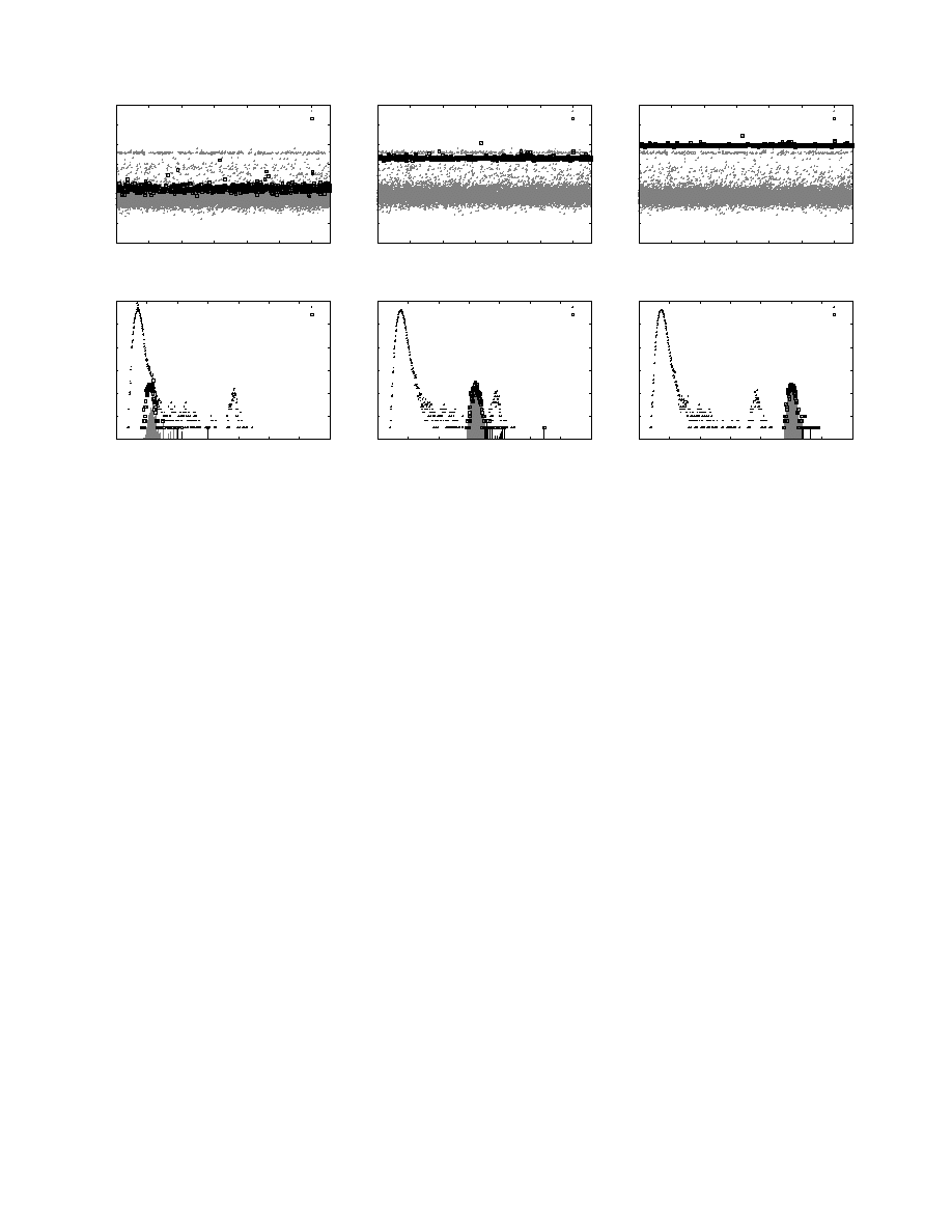
Figure 1: Base (top) and inverse (bottom) frequency distributions of fingerprints over a 20,000 packet window observed at three
different time epochs: Epoch 205 corresponds to the appearance of 22 Witty worm packets, Epoch 215 to 132 packets, and Epoch
225 to 242 packets. The fingerprints appearing in all worm packets are shown using the square points. The gray bars under the
inverse distribution show regions containing fingerprints that have been displaced with respect to the previous time epoch by a large
value. Note that the inverse distribution shows the presence of the worm from Epoch 205 itself.

2.

CASE STUDY

The benefits of inverse distributions vis-a-vis base distributions

are highlighted by a case study that we conducted. We captured
packets on our research network (a /24 address range subnetted
from a Class B address, with about 60 hosts active at any one time)
over a 15-minute period. The packet trace, containing roughly
75,000 incoming and outgoing UDP and TCP packets, corresponded
to a variety of applications including web server requests and re-
sponses, interactions with mail servers using POP and IMAP, file
server access, and IM and chat traffic.

Into this trace, we synthetically injected UDP packets correspond-

ing to two well-known worms: the SQL Slammer worm and the
W32.Witty worm. Packets containing the SQL Slammer worm ap-
peared throughout the trace at a relatively low frequency (1 worm
packet for every 64 data packets) and correspond to the presence
of known worms in network traffic; typically, such worm packets
continue to propagate long after the worm has been detected and
counteracted. The Witty worm packets correspond to a new, as yet
unknown worm, and start appearing 20,000 packets into the trace
at a higher rate: 1 worm packet for every 8 data packets. Our ob-
jective was to examine whether any signals indicative of this new
worm could be discerned by analyzing the base and inverse distri-
butions of packet contents and whether one distribution presented
any advantages over the other.

To build these distributions, we represent packet contents as in

earlier work by a bag of “shingles” [1] denoting different sub-
strings. We derive a smaller p-bit “fingerprint” for each overlap-
ping k-byte segment (“shingle”) of the packet body, one for each
byte boundary. Each packet is represented by the set of finger-
prints it contains, and the contents of all packets seen by a router
is compactly captured by either the base or the inverse frequency

distribution of these fingerprints. Intuitively, two packets exhibit-
ing byte-level similarity would share a set of shingles, while two
dissimilar packets would not. Thus, as the system sees an increas-
ing number of worm packets, we would expect the fingerprints de-
rived from such packets to appear with frequencies higher than the
other fingerprints. These “frequency gaps” are manifested differ-
ently in the base and inverse distributions, leading to differences in
how suitable a particular distribution might be in identifying pack-
ets that are possibly malicious (in the sense that they contain high-
frequency fingerprints, hence the corresponding shingles).

Fig. 1 shows the base (top) and inverse (bottom) frequency dis-

tributions (with k

= 20 and p = 16) over a 20,000 packet window;

the y-axis in both plots uses the log scale. The plots correspond
to three time instants: (Epoch 205) where 22 packets of the Witty
worm have been seen, (Epoch 215) with 132 worm packets, and
(Epoch 225) with 242 worm packets.

Signal in the base distribution.

The base distribution plots

clearly show the movement of the fingerprints shared by all worm
packets (shown using square points), corresponding to the frequency
gap described above. Although the movement is present through-
out, it is only at Epoch 225 that the highest frequency fingerprints
in the base distribution do in fact correspond to the worm.

Systems like EarlyBird, Autograph, and Polygraph distinguish

among the fingerprints based on a frequency threshold: fingerprints
that appear more frequently than this threshold are tagged as poten-
tially malicious, and those below are not. Such approaches neces-
sarily entail a tradeoff between early detection of new worm traffic
and the likelihood of false positives; the former argues for lower fre-
quency thresholds while the latter requires higher thresholds. Even
with 40-byte substrings, only a very small number of which can
appear over any reasonable observation window, EarlyBird suffers

from false positives and requires a manually created “whitelist” of
good substrings known to occur frequently.

To avoid false positives without using whitelists, one would need

to wait for a time instant where the frequency of the worm finger-
prints exceeds that of previously known sources of content similar-
ity (the SQL Slammer worm in this case). Not only does this delay
detection to Epoch 225 in our case, but also note that whether or not
a new worm’s fingerprints ever correspond to the most frequently
occuring set depends upon the relative rate with which the worm
packets appear during the time window captured by the distribu-
tion. In particular, if the rate of Witty worm packets remains below
that of the Slammer worm, detection mechanisms that analyze the
most prevalent fingerprints will not yield good results. Stealthy
worm attacks are particularly prone to this phenomenon: their rel-
ative rate may never exceed the threshold required for sufficiently
discriminating detection.

Signal in the inverse distribution.

In contrast, the inverse dis-

tribution plots in the bottom half of Fig. 1 appear not to suffer from
these problems. Some additional explanation is necessary about
the nature of these plots. The envelope made up from one or more
“bumps” corresponds to the inverse distribution I

( f ), which tracks

for a given frequency f , the number of fingerprints that appear with
that frequency. The contribution of the worm fingerprints to this
count at each column is shown using the square points. Finally, the
gray shaded regions under the inverse distribution curve show con-
tributions from those fingerprints that have incurred displacements
from the previous time epoch of more than a certain threshold. In-
formally, these regions show the portion of the frequency spectrum
occupied by fast-moving fingerprints.

The inverse distribution plots show the emergence of the new

worm packets in a clearer, unambiguous, and rate-insensitive fash-
ion. At Epoch 215, the new worm packets are discernible because
of the creation of a new “bump” between the two originally present
at Epoch 205 and earlier. One might argue that a similar feature can
also be detected from the base distribution at the same time instant,
particularly if we look for gaps in the frequency distribution instead
of just focusing on the highest frequency fingerprints. Note how-
ever that unlike in the base distribution, in the inverse distribution
at Epoch 205, the worm is already noticeable after only 22 pack-
ets: here, their presence distorts the first bump in a way consistent
with a new bump breaking away from the original one. Moreover,
for fast spreading worms, tracking the various fingerprint displace-
ments (the gray regions in the plots) may in fact yield a more re-
sponsive detector that raises an alert even before any perceptible
distortion is observed in the inverse distribution envelope.

Although the case study looks at a small amount of network data

and synthetic worm propagation behaviors, it highlights the poten-
tial of using inverse distributions: the analysis of the structure and
location of the bumps in this distribution appears to provide a highly
discriminating, responsive mechanism for characterizing different
sources of content similarity.

3.

TRACKING FEATURES INDICATING
CONTENT SIMILARITY

We consider a network element that at time t has access to a

history of base distributions B

t

−m+1

,B

t

−m+2

,...,B

t

and a history

of inverse distributions I

t

−k+1

,I

t

−k+2

,...,I

t

(k can be larger than

m because inverse distributions are typically more compact). The
distributions store information about packet fingerprints observed
over a sliding fixed-size time window: since packets seen in the
past cannot be retained, each distribution is necessarily approxi-
mate (we use exponential weighting to “forget” packets at the trail-

ing edge of the window). Comparing the frequency value of a fin-
gerprint across the sequence of base distributions allows us to com-
pute its displacement and thereby construct the gray regions shown
in Fig. 1. We want to (1) characterize the bumps in the inverse
distribution (in terms of their number and location, the set of fin-
gerprints that make up the bumps, etc.); and (2) track these bumps
over time as they appear, move, and disappear.

Below, we sketch several approaches we have been pursuing to-

wards this objective; we have focused so far on detection ability
and robustness concerns rather than implementation efficiency. The
approaches rely on a probabilistic model for the shape of possible
inverse distributions.

3.1

Modeling the Inverse Distribution

We start by modeling the inverse distribution for background

traffic in the absence of any packet groups exhibiting content simi-
larity, and then extend it to account for such groups.

Background traffic.

Each packet’s content is represented by a

set of fingerprints. Our basic model assumes that the fingerprints
are produced by a uniform distribution. With p-bit fingerprints,
there are at most N

F

= 2

p

different fingerprints. For ideal finger-

printing mechanisms, a random shingle is hashed to fingerprint i
with probability p

(i) = p = 1/N

F

.

Since the probability of each fingerprint is uniform and inde-

pendent of the previous ones, the probability that some particular
fingerprint i has appeared k times in the total of n fingerprints seen
at the router is given by the binomial distribution:

b

(k,n, p(i)) =

n
k

p

(i)

k

(1 − p(i))

n

≈

(np)

k

k!

e

−np

= p(k,np),

(1)

where the approximation by the Poisson distribution p

(k,np) is

valid when, as in our case, n is very large and p

(i) = p = 1/N

F

is small such that

λ = np is of moderate magnitude. Thus, the

expected number of fingerprints that appear k times is E

F

,n

(k) =

N

F

p

(k,np), an observation confirmed with real data.

Adding a single packet group to the background.

We

assume that the group is made up of identical packets, and corre-
sponds to N

G

distinct fingerprints (the “group fingerprints”). Thus,

when a packet from the group is observed, the inverse distribution
increments by one for each of these N

G

fingerprints.

If there are n

G

observations of each group fingerprint and n ob-

servations of background traffic fingerprints, the expected number
of fingerprints that appear k times is:

(i) For the N

F

−N

G

fingerprints that are not present in the group

packets, but exist in the background traffic, following Eq. 1,

E

F

−G,n

(k) = (N

F

− N

G

) p(k,np).

(ii) Fingerprints that are present in the group packet will con-

tribute to the inverse distribution each time they are observed,
say n

G

times. Necessarily, k

≥ n

G

, with n

G

contributed by

group packets, and k

− n

G

contributed by the background.

There are N

G

of these fingerprints, so

E

G

,n

(k) = N

G

p

(k − n

G

, np)

for

k

≥ n

G

.

Combining the two cases, E

F

,n

(k) = (N

F

−N

G

) p(k,np)+N

G

p

(k−

n

G

, np) when k ≥ n

G

, and N

F

p

(k,np) when k < n

G

. Intuitively,

the resulting inverse distribution consists of a Poisson component
(bump) for the background and a shifted one for the group.

Generalizing to

L

> 1

groups.

There may be up to 2

L

bumps,

0

2

4

6

8

10

12

14

16

18

20

0

1

2

3

4

5

6

7

8

9 10 11 12 13 14

log(# Fingerprints)

Median Frequency

Epoch 205

all traffic

worm traffic

Figure 2: “Squashed” inverse distribution of fingerprints over a
100 packet window. The fingerprints appearing in Witty worm
packets are shown using the square points. Note the clear sep-
aration between worm and background fingerprints.

since two or more groups may contain common fingerprints and
these fingerprints will then appear more often as compared to the
other fingerprints that are not common. Such combinatorics needs
to be carefully modeled, but the overall structure of the model stays
the same as for the single group case above: the inverse distribution
is made up out of a primary background bump and some number of
content similarity-induced secondary bumps.

“Squashed” inverse distributions.

The above model assumed

that the observation window (measured in number of fingerprints)
over which the inverse distribution was being computed was much
larger than the overall universe of fingerprints. Analyzing the in-
verse distributions that result under a different set of assumptions,
specifically where the reverse is true, can also be beneficial.

Intuitively, when the fingerprint universe is significantly larger

than the observation epoch, one expects a fingerprint to appear at
most once in background traffic. However, fingerprints correspond-
ing to worm packets should appear with a frequency determined by
the number of worm packets observed in the observation epoch.
Thus, given a sufficiently large observation epoch over which one
observes multiple worm packets, and a fingerprint universe that is
significantly larger, one can create inverse distributions where the
fingerprints that appear only in the background traffic are essen-
tially squashed against the y-axis.

Such squashed inverse distributions potentially permit earlier de-

tection of malicious traffic. Fig. 2 shows the inverse distribution for
the trace in Section 2 built using the median frequency value of a
fingerprint over three epochs each corresponding to 100 packets.
Each fingerprint was of size 18 bits resulting in a universe of size
2

18

; in comparison, the number of fingerprint observations in an

epoch was around 30,000. The inverse distribution corresponds to
the leftmost Epoch 205 in Fig. 1, but in contrast shows the presence
of the worm packets more clearly.

Note that these benefits come with costs: (1) increased memory

requirements for storing the distributions over a larger universe of
fingerprints; and (2) increased sensitivity to benign temporary ap-
pearances of content similarity because of the compressed observa-
tion windows. In practice, one would likely want to work with both
the squashed and the original inverse distributions.

3.2

Bump Characteristics and Motion

Guided by the models above, we analyze the base and inverse

distribution data to infer information about the presence of content
similarity groups in network traffic, and the set of fingerprints that
define these groups. We have been exploring both direct and indi-

rect approaches towards this goal. The output in either case is the
identification of one or more sets of fingerprints, whose emergence,
movement, and disappearance is tracked over time.

The direct approach, which we have been experimenting with in

the context of squashed inverse distributions, looks for fingerprints
that appear with larger than expected frequency over a number of
observation epochs. These fingerprints can be identified either us-
ing a simple thresholding test on a robust statistic such as the me-
dian, or a probabilistic framework similar to sequential hypothe-
sis testing. Fingerprints that appear with similar frequencies are
grouped into the same set.

The indirect approach first detects features (bumps) in the in-

verse distribution and then correlates these features with the set
of fingerprints that most likely resulted in their presence. For the
general inverse distribution, the features correspond to the Poisson
bumps. Although ideally we would like to directly estimate the
Poisson parameters, to simplify the analysis we model the loga-
rithm of the distribution as a linear combination of normal distri-
butions (the Gaussian mixture model); each Poisson distribution is
approximated by a Gaussian function

G

k

(

µ,σ) and is associated

with a scale parameter a. Our estimation problem is one of deter-
mining these parameters for some number of Gaussian functions,
say W

, that best approximates the real data according to a mixture

model:

˜

E

F

,n

(k) = log(1 + E

F

,n

(k)) ≈

W

∑

i

=1

a

i

G

k

(

µ

i

,

σ

i

).

The value of W is unknown a priori, so it also needs to be esti-

mated. At first glance, this problem is well-studied: there is a huge
body of literature on Gaussian mixture modeling with unknown
numbers of components, including integrated model selection and
estimation approaches (e.g., [6]). However, we have found these
approaches to be non-robust: small fluctuations in the inverse dis-
tributions across adjoining time epochs produce widely different
numbers of components. Consequently, we have been pursuing
a two-step procedure where we first estimate W using domain-
specific mechanisms, and then compute the parameters of the W
components using standard statistical techniques.

Estimating

W

, the number of bumps.

Since a bump evolves

over time in a well-known pattern modulo statistical fluctuations,
we estimate W by tracking the “flow” of the inverse distribution
over time. The correspondence between two inverse histograms is
used to obtain a displacement field, either at the detailed level of
individual fingerprints (particularly those that incur large displace-
ments), or at the level of the inverse distribution envelope. These
displacements are then tracked to determine the number of bumps,

W , and their locations.

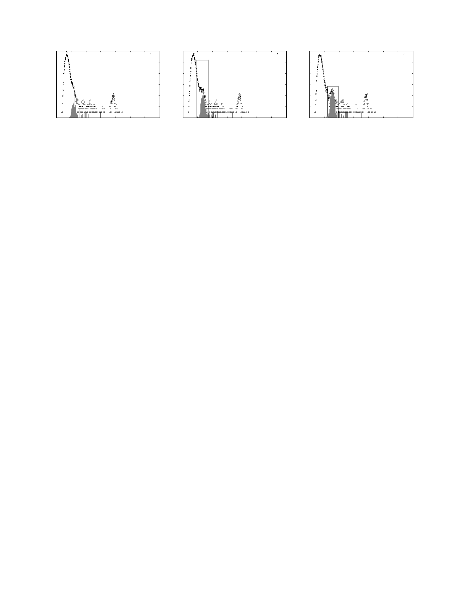
Tracking fast-moving fingerprints. As Fig. 1 shows, the motion of
the bump denoting the worm packets is accompanied by the appear-
ance at the corresponding region of frequency values, of a group of
fingerprints that have incurred large frequency changes with refer-
ence to an earlier time instant. Thus, computing for each frequency
value, the number of fingerprints that have arrived there because of
a large increment in their frequency, can help identify portions of
the frequency range where a bump is located.

One can additionally track the patterns of how these regions

themselves evolve over time to rule out potential false positives.
For example, we expect a worm bump moving to the right to re-
sult in a decrease in the number of fast moving fingerprints at the
previous location and an increase in the new location.

Fig. 3 shows the output of a tracker program developed using

these principles. Note that as we had speculated in Section 2, the

0

2

4

6

8

10

12

0

100

200

300

400

500

600

700

log(# Fingerprints)

Frequency

Epoch 205

all traffic

0

2

4

6

8

10

12

0

100

200

300

400

500

600

700

log(# Fingerprints)

Frequency

Epoch 206

all traffic

0

2

4

6

8

10

12

0

100

200

300

400

500

600

700

log(# Fingerprints)

Frequency

Epoch 207

all traffic

Figure 3: Tracking fast-moving fingerprints can help identify emergence of bumps indicating new sources of content similarity. For
the case study described in Section 2, one can, fully automatically, detect presence of the group of Witty worm packets at Epoch 206,
after only 33 worm packets have been seen.

emergence of the bump can be flagged (shown by the boxed re-
gion) with sufficient confidence well before the bump has com-
pletely separated from its “parent.” In this case, we are able to
flag the appearance of a new source of content similarity at Epoch
206, after only 33 copies of the Witty worm packet were observed.

Tracking changes in the inverse distribution envelope. Direct track-
ing of fingerprint displacements does not pick up stealthy worms,
whose propagation rate stays below a threshold. Such cases can
still be detected by tracking changes in the inverse distribution en-
velope: rate of worm propagation can only affect how quickly these
changes happen, but cannot prevent them from happening.

We use a Bayesian formulation for defining the best correspon-

dence between two inverse distribution envelopes I

t

and I

t

−1

. As

bumps appear or disappear they cause a portion of inverse distribu-
tion to move to the left or the right. Thus, the correspondence can
be defined in terms of the displacement (in terms of frequency) seen
by each point in the I

t

−1

envelope for the latter to have transformed

into the I

t

envelope. A particular assignment of displacement val-

ues is more probable the closer the I

t

−1

envelope comes to the I

t

envelope after applying that displacement. We would also like (1)
for a packet group arrival/departure to cause as few displacement
changes over the prior model as possible; (2) to not skip matches
for regions of the inverse distribution; and (3) to have a slight pref-
erence towards a displacement of zero. Each of these conditions
can be factored into the formulation by introducing additional bi-
ases into the expression governing the probability of a particular
assignment of displacement values.

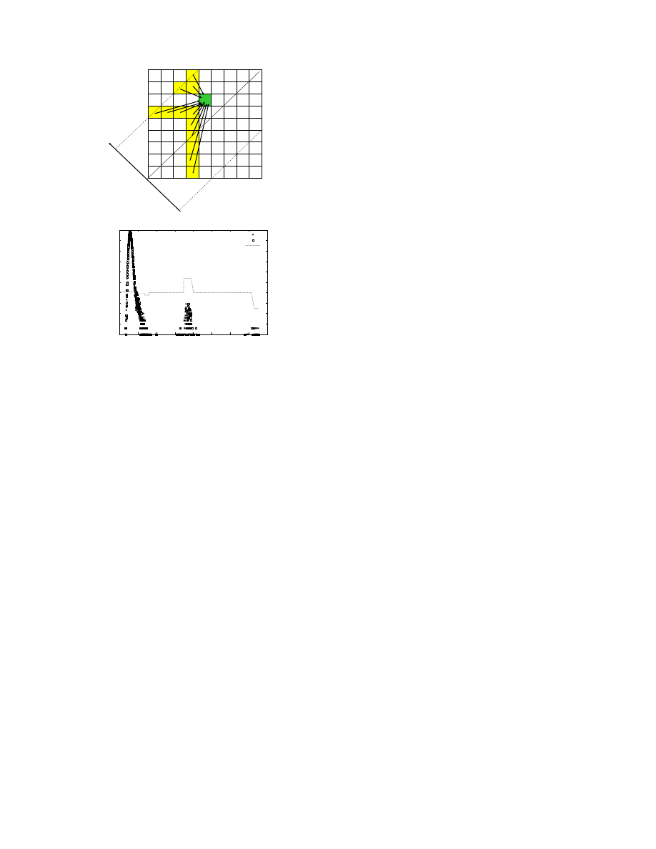
A dynamic programming scheme can be used to obtain the op-

timal displacement value associated with each point in the I

t

−1

inverse envelope (see Fig. 4). Note that both positive and nega-
tive displacement values are explored to support movements of the
point to the right or left. Fig. 4 (bottom) shows the optimal dis-
placement fields for two consecutive time epochs from a different
trace: note the positive and negative steps in the displacement fields
corresponding to the two non-background bumps (one moving to
the right, and one to the left).

Estimating Parameters of the

W

Gaussians.

This can be

done in a relatively straightforward manner once we know W . The
parameters of the Gaussian components can be estimated, among
other methods, by using a Bayesian framework involving max-
imum likelihood and the Expectation Maximization (EM) algo-
rithm [4]. The initial guesses of the a and

µ parameters are based

on the results of the change detection procedures above. Addi-
tional domain knowledge (e.g., the relative sizes of the bumps, their

spread, and inter-bump spacings) can be easily incorporated within
the Bayesian formulation.

4.

DISCUSSION

The algorithms outlined in Section 3 only characterize the fea-

tures of the inverse distribution of packet contents. Several addi-
tional issues need to be addressed before this information can be
profitably incorporated into network security tools:

Relating bumps to packet groups.

A feature in the inverse

distribution corresponds to a set of fingerprints that are part of a
content similarity group; however, this set alone does not always
uniquely identify a group of packets that share content (because
two groups of packets can have overlapping fingerprints).

To address this issue, we have been pursuing an approach that

uses the Gaussian mixture parameters to associate with each fin-
gerprint f , the probability, p

( f ,i), that it belongs to the i’th of the

W components. These probabilities in turn help estimate the frac-

tion of a packet’s content that corresponds to each of the compo-
nents. For a packet with fingerprint set

{ f

1

,..., f

n

}, the fraction of

its content that corresponds to Gaussian component i is given by
x

i

= ∑

n

j

=1

p

( f

j

,i).

Given these fractions,

(x

1

,...,x

W

), one can view the packet as a

point in W -dimensional space falling on the hyperplane that inter-
sects each of the axes at unit distance from the origin. Intuitively,
packets exhibiting content-level similarity end up getting clustered
on this hyperplane. Clusters that contain higher than a threshold of
their content associated with one or more non-background Gaus-
sian components define a packet group of interest. Experiments on
small-to-medium sized traces support this intuition: clusters that
form are clearly separated, and each cluster does correspond to
packets that exhibit content similarity.

A variety of algorithms are possible for detecting such clusters

at run time, and for characterizing information about each clus-
ter (e.g., cluster centroid, spread, exemplar packets for the cluster,
etc.). Note that as new components emerge or existing ones disap-
pear, cluster statistics need to be transformed to correspond to the
new feature space that now gets defined.

Distinguishing benign and malicious packet groups.

Not

all packet groups that exhibit content-level similarity are malicious.
In fact, such similarity may be expected in several situations, e.g.,
in the request and response traffic of a popular web server respond-
ing to several client requests. Two mechanisms can help reduce
the likelihood of raising false alerts. First, it may be possible,
as in the above situation, to identify expected sources of similar-

?

i-k

i-1 i=5

j+1

j=7

j-1

Displacement

0

-5

D=5

Ι

t-1

Ι

t

1

2

3

4

5

6

7

8

9

10

11

0

200

400

600

800

1000 1200 1400 1600

log(# Fingerprints)

Frequency

t1
t2

flow

Figure 4: Dynamic programming structure (top) and the dis-
placement field (“flow”) across two epochs (bottom).

ity, which can then be simply factored out from subsequent anal-
ysis. Second, content analyses can be complemented with tradi-
tional header-based or flow-based statistics to refine the detection
procedure. For example, one expects computer worm propagation
patterns to show themselves as changes in the IP source and des-
tination node connectivity structure, which would now contain a
higher than expected number of edges between nodes that have pre-
viously not been big contributors to overall traffic. Such changes
can be detected by extending recent stream-based traffic analyses
that have identified “heavy hitter” sources and flows [5, 11, 2]. The
EarlyBird system uses a simpler variant of this idea, by tracking IP
source addresses that produce a large amount of traffic.

Implementation efficiency.

Given the relatively heavy-weight

analyses described in Section 3, one might be concerned whether
such analyses can ever be used at multi-Gbps line rates. Several
possibilities exist for reducing the computational cost and memory
requirements of such analyses. First, cheaper header analyses can
be used to filter packets for content analysis. Second, while the
per-packet shingling procedure itself needs to run at line rates, the
analysis of the inverse distribution can happen at larger time granu-
larities (reflecting the aggregate impact of a group of packets). The
shingling procedure itself is very regular and can benefit from a
hardware assist. Third, the iterative nature of the algorithms may
permit combining the iteration steps with incremental data updates.

Moreover, both the shingling step and the algorithms themselves

can benefit from recent advances in sketching and sampling tech-
niques developed for data stream analysis [12, 3]. Recently devel-
oped stream algorithms for estimating individual points, quantiles
and heavy-hitters to certain approximations [3] as well as associ-
ated communication complexity results [10] can all be extended to
the inverse distribution domain. Note also that because the inverse

distribution is smaller in size than its base counterpart, it lends itself
to the use of more sophisticated algorithms for mixture analysis,
clustering, or change detection of the kind needed by our approach.

Other uses of inverse distribution analyses on content.

In

addition to detecting sources of content similarity, inverse distribu-
tions of packet contents appear to have potential as compact signa-
tures for specific (a priori known) kinds of content. For example,
one can imagine such analyses being performed to detect whether
copyrighted music or other media data is being transmitted out of
an organization’s networks. Prior work on application-level sig-
natures based on content (eg., [14]) may also be extended to use
inverse distributions.

Finally, note that although this paper has viewed packet content

as a sequence of bytes, the techniques are equally applicable to
other representations. This observation can enable use of inverse
distribution analyses for spam detection (where content is repre-
sented as a set of keywords) and for detecting polymorphic viruses
and worms (where content is represented as a set of distinguished
instruction sequences).

5.

REFERENCES

[1] A. Z. Broder, S. C. Glassman, M. S. Manasse, and G. Zweig.

Syntactic clustering of the web. In Proc. WWW Conf., 1997.

[2] G. Cormode, F. Korn, S. Muthukrishnan, and D. Srivastava.

Diamonds in the rough: Finding hierarchical heavy hitters in
multidimensional data. In Proc. SIGMOD, 2004.

[3] M. Datar and S. Muthukrishnan. Computing rarity and

similarity over data streams. In Proceedings ESA, 2002.

[4] R. Duda, P. Hart, and D. Stork. Pattern Classification. Wiley

Interscience, 2nd Edition, 2000.

[5] C. Estan and G. Varghese. New directions in traffic

measurement and accounting. In Proc. ACM SIGCOMM
Internet Measurement Workshop, 2001.

[6] M. A. T. Figueiredo and A. K. Jain. Unsupervised learning of

finite mixture models. IEEE Trans. Pattern Analysis and
Machine Intelligence, 24(3):381–396, 2002.

[7] J. Jung, V. Paxson, A. W. Berger, and H. Balakrishnan. Fast

portscan detection using sequential hypothesis testing. In
Proc. IEEE Security and Privacy, 2004.

[8] J. O. Kephart and W. C. Arnold. Automatic extraction of

computer virus signatures. In Proc. 4th Intl. Virus Bulletin
Conf., 2001.

[9] H. A. Kim and B. Karp. Autograph: Toward automatic

distributed worm signature detection. In Proc. USENIX
Security Symp., 2004.

[10] K. Levchenko, R. Paturi, and G. Varghese. On the difficulty

of scalably detecting network attacks. In Proc. ACM Symp.
on Computer and Communication Security, 2004.

[11] G. Manku and R. Motwani. Approximate frequency counts

over data streams. In Proc. VLDB, 2002.

[12] S. Muthukrishnan. Data stream algorithms and applications.

Url:http://www.cs.rutgers.edu/˜muthu/
stream-1-1.ps

.

[13] J. Newsome, B. Karp, and D. Song. Polygraph:

Automatically generating signatures for polymorphic worms.
In Proc. IEEE Security and Privacy, 2005.

[14] S. Sen, O. Spatscheck, and D. Wang. Accurate, scalable

in-network identification of P2P traffic using application
signatures. In Proc. WWW Conf., 2004.

[15] S. Singh, C. Estan, G. Varghese, and S. Savage. Automated

worm fingerprinting. In Proc. OSDI, 2004.