Norbury General relativity and cosmology for undergraduates (Wisconsin lecture notes, 1997)(116s)

GENERAL RELATIVITY &

COSMOLOGY

for Undergraduates

Professor John W. Norbury

Physics Department

University of Wisconsin-Milwaukee

P.O. Box 413

Milwaukee, WI 53201

1997

Contents

NEWTONIAN COSMOLOGY

1.1

Introduction . . . . . . . . . . . . . . . . . . . . . . . . . . . .

1.2

Equation of State . . . . . . . . . . . . . . . . . . . . . . . . .

1.2.1

Matter . . . . . . . . . . . . . . . . . . . . . . . . . . .

1.2.2

Radiation . . . . . . . . . . . . . . . . . . . . . . . . .

1.3

Velocity and Acceleration Equations . . . . . . . . . . . . . .

1.4

Cosmological Constant . . . . . . . . . . . . . . . . . . . . . .

1.4.1

Einstein Static Universe . . . . . . . . . . . . . . . . .

APPLICATIONS

2.1

Conservation laws

. . . . . . . . . . . . . . . . . . . . . . . .

2.2

Age of the Universe

. . . . . . . . . . . . . . . . . . . . . . .

2.3

Inflation . . . . . . . . . . . . . . . . . . . . . . . . . . . . . .

2.4

Quantum Cosmology . . . . . . . . . . . . . . . . . . . . . . .

2.4.1

Derivation of the Schr¨

odinger equation . . . . . . . . .

2.4.2

Wheeler-DeWitt equation . . . . . . . . . . . . . . . .

2.5

Summary . . . . . . . . . . . . . . . . . . . . . . . . . . . . .

2.6

Problems

. . . . . . . . . . . . . . . . . . . . . . . . . . . . .

2.7

Answers . . . . . . . . . . . . . . . . . . . . . . . . . . . . . .

2.8

Solutions

. . . . . . . . . . . . . . . . . . . . . . . . . . . . .

TENSORS

3.1

Contravariant and Covariant Vectors . . . . . . . . . . . . . .

3.2

Higher Rank Tensors . . . . . . . . . . . . . . . . . . . . . . .

3.3

Review of Cartesian Tensors . . . . . . . . . . . . . . . . . . .

3.4

Metric Tensor . . . . . . . . . . . . . . . . . . . . . . . . . . .

3.4.1

Special Relativity . . . . . . . . . . . . . . . . . . . . .

3.5

Christoffel Symbols . . . . . . . . . . . . . . . . . . . . . . . .

CONTENTS

3.6

Christoffel Symbols and Metric Tensor . . . . . . . . . . . . .

3.7

Riemann Curvature Tensor . . . . . . . . . . . . . . . . . . .

3.8

Summary . . . . . . . . . . . . . . . . . . . . . . . . . . . . .

3.9

Problems

. . . . . . . . . . . . . . . . . . . . . . . . . . . . .

3.10 Answers . . . . . . . . . . . . . . . . . . . . . . . . . . . . . .

3.11 Solutions

. . . . . . . . . . . . . . . . . . . . . . . . . . . . .

ENERGY-MOMENTUM TENSOR

4.1

Euler-Lagrange and Hamilton’s Equations . . . . . . . . . . .

4.2

Classical Field Theory . . . . . . . . . . . . . . . . . . . . . .

4.2.1

Classical Klein-Gordon Field . . . . . . . . . . . . . .

4.3

Principle of Least Action

. . . . . . . . . . . . . . . . . . . .

4.4

Energy-Momentum Tensor for Perfect Fluid . . . . . . . . . .

4.5

Continuity Equation . . . . . . . . . . . . . . . . . . . . . . .

4.6

Interacting Scalar Field

. . . . . . . . . . . . . . . . . . . . .

4.7

Cosmology with the Scalar Field . . . . . . . . . . . . . . . .

4.7.1

Alternative derivation . . . . . . . . . . . . . . . . . .

4.7.2

Limiting solutions . . . . . . . . . . . . . . . . . . . .

4.7.3

Exactly Solvable Model of Inflation . . . . . . . . . . .

4.7.4

Variable Cosmological Constant . . . . . . . . . . . . .

4.7.5

Cosmological constant and Scalar Fields . . . . . . . .

4.7.6

Clarification . . . . . . . . . . . . . . . . . . . . . . . .

4.7.7

Generic Inflation and Slow-Roll Approximation . . . .

4.7.8

Chaotic Inflation in Slow-Roll Approximation . . . . .

4.7.9

Density Fluctuations . . . . . . . . . . . . . . . . . . .

4.7.10 Equation of State for Variable Cosmological Constant

4.7.11 Quantization . . . . . . . . . . . . . . . . . . . . . . .

4.8

Problems

. . . . . . . . . . . . . . . . . . . . . . . . . . . . .

EINSTEIN FIELD EQUATIONS

5.1

Preview of Riemannian Geometry . . . . . . . . . . . . . . . .

5.1.1

Polar Coordinate . . . . . . . . . . . . . . . . . . . . .

5.1.2

Volumes and Change of Coordinates . . . . . . . . . .

5.1.3

Differential Geometry . . . . . . . . . . . . . . . . . .

5.1.4

1-dimesional Curve . . . . . . . . . . . . . . . . . . . .

5.1.5

2-dimensional Surface . . . . . . . . . . . . . . . . . .

5.1.6

3-dimensional Hypersurface . . . . . . . . . . . . . . .

5.2

Friedmann-Robertson-Walker Metric . . . . . . . . . . . . . .

5.2.1

Christoffel Symbols . . . . . . . . . . . . . . . . . . . . 101

CONTENTS

5.2.2

Ricci Tensor . . . . . . . . . . . . . . . . . . . . . . . . 102

5.2.3

Riemann Scalar and Einstein Tensor . . . . . . . . . . 103

5.2.4

Energy-Momentum Tensor

. . . . . . . . . . . . . . . 104

5.2.5

Friedmann Equations

. . . . . . . . . . . . . . . . . . 104

5.3

Problems

. . . . . . . . . . . . . . . . . . . . . . . . . . . . . 105

Einstein Field Equations

107

Weak Field Limit

109

Lagrangian Methods

111

CONTENTS

Chapter 1

NEWTONIAN
COSMOLOGY

1.1

Introduction

Many of the modern ideas in cosmology can be explained without the need
to discuss General Relativity. The present chapter represents an attempt to
do this based entirely on Newtonian mechanics. The equations describing
the velocity (called the Friedmann equation) and acceleration of the universe
are derived from Newtonian mechanics and also the cosmological constant
is introduced within a Newtonian framework. The equations of state are
also derived in a very simple way. Applications such as conservation laws,
the age of the universe and the inflation, radiation and matter dominated
epochs are discussed.

1.2

Equation of State

In what follows the equation of state for non-relativistic matter and radiation
will be needed. In particular an expression for the rate of change of density,

ρ, will be needed in terms of the density ρ and pressure p. (The definition

≡

, where t is time, is being used.) The first law of thermodynamics is

dU + dW = dQ

(1.1)

where U is the internal energy, W is the work and Q is the heat transfer.
Ignoring any heat transfer and writing dW = F dr = pdV where F is the

CHAPTER 1. NEWTONIAN COSMOLOGY

force, r is the distance, p is the pressure and V is the volume, then

dU =

−pdV.

(1.2)

Assuming that ρ is a relativistic energy density means that the energy is
expressed as

U = ρV

(1.3)

from which it follows that

U = ˙

ρV + ρ ˙

V =

−p ˙V

(1.4)

where the term on the far right hand side results from equation (1.2). Writing

∝ r

implies that

V
V

= 3

r
r

. Thus

ρ =

−3(ρ + p)

˙r

(1.5)

1.2.1

Matter

Writing the density of matter as

ρ =

4
3

πr

(1.6)

it follows that

≡

dρ

˙r =

−3ρ

˙r

(1.7)

so that by comparing to equation (1.5), it follows that the equation of state
for matter is

p = 0.

(1.8)

This is the same as obtained from the ideal gas law for zero temperature.
Recall that in this derivation we have not introduced any kinetic energy, so
we are talking about zero temperature.

1.2.2

Radiation

The equation of state for radiation can be derived by considering radiation
modes in a cavity based on analogy with a violin string [12]. For a standing
wave on a string fixed at both ends

L =

nλ

(1.9)

1.3. VELOCITY AND ACCELERATION EQUATIONS

where L is the length of the string, λ is the wavelength and n is a positive
integer (n = 1, 2, 3.....). Radiation travels at the velocity of light, so that

c = f λ = f

(1.10)

where f is the frequency. Thus substituting f =

c into Planck’s formula

U = ¯

hω = hf , where h is Planck’s constant, gives

U =

nhc

∝ V

−1/3

(1.11)

Using equation (1.2) the pressure becomes

≡ −

(1.12)

Using ρ = U/V , the radiation equation of state is

p =

ρ.

(1.13)

It is customary to combine the equations of state into the form

p =

(1.14)

where γ

≡ 1 for radiation and γ ≡ 0 for matter. These equations of state

are needed in order to discuss the radiation and matter dominated epochs
which occur in the evolution of the Universe.

1.3

Velocity and Acceleration Equations

The Friedmann equation, which specifies the speed of recession, is obtained
by writing the total energy E as the sum of kinetic plus potential energy
terms (and using M =

4
3

πr

ρ )

E = T + V =

m ˙r

− G

M m

−

8πG

ρ)

(1.15)

where the Hubble constant H

≡

r
r

, m is the mass of a test particle in the

potential energy field enclosed by a gas of dust of mass M , r is the distance
from the center of the dust to the test particle and G is Newton’s constant.

CHAPTER 1. NEWTONIAN COSMOLOGY

Recall that the escape velocity is just v

escape

2GM

8πG

ρr

, so that

the above equation can also be written

˙r

= v

escape

− k

− 2

(1.16)

with k

≡ −

. The constant k

can either be negative, zero or positive

corresponding to the total energy E being positive, zero or negative. For
a particle in motion near the Earth this would correspond to the particle
escaping (unbound), orbiting (critical case) or returning (bound) to Earth
because the speed ˙r would be greater, equal to or smaller than the escape
speed v

escape

. Later this will be analagous to an open, flat or closed universe.

Equation (1.15) is re-arranged as

8πG

ρ +

.13

− 3

(1.17)

Defining k

≡ −

and writing the distance in terms of the scale factor R

and a constant length s as r(t)

≡ R(t)s, it follows that

r
r

R
R

and

r
r

R
R

giving the Friedmann equation

≡ (

)

8πG

−

(1.18)

which specifies the speed of recession. The scale factor is introduced because
in General Relativity it is space itself which expands [19]. Even though this
equation is derived for matter, it is also true for radiation. (In fact it is also
true for vacuum, with Λ

≡ 8πGρ

vac

, where Λ is the cosmological constant

and ρ

vac

is the vacuum energy density which just replaces the ordinary den-

sity. This is discussed later.) Exactly the same equation is obtained from
the general relativistic Einstein field equations [13]. According to Guth [10],
k can be rescaled so that instead of being negative, zero or positive it takes
on the values

−1, 0 or +1. From a Newtonian point of view this corresponds

to unbound, critical or bound trajectories as mentioned above. From a geo-
metric, general relativistic point of view this corresponds to an open, flat or
closed universe.

In elementary mechanics the speed v of a ball dropped from a height r

is evaluated from the conservation of energy equation as v =

√

2gr, where

g is the acceleration due to gravity. The derivation shown above is exactly
analagous to such a calculation. Similarly the acceleration a of the ball is
calculated as a = g from Newton’s equation F = m¨

r, where F is the force

1.4. COSMOLOGICAL CONSTANT

and the acceleration is ¨

≡

. The acceleration for the universe is obtained

from Newton’s equation

−G

M m

= m¨

r.13

− 5

(1.19)

Again using M =

4
3

πr

ρ and

r
r

R
R

gives the acceleration equation

≡

−

4πG

ρ.

(1.20)

However because M =

4
3

πr

ρ was used, it is clear that this acceleration

equation holds only for matter. In our example of the falling ball instead of
the acceleration being obtained from Newton’s Law, it can also be obtained
by taking the time derivative of the energy equation to give a =

= v

dv
dr

(

√

2gr)(

√

) = g. Similarly, for the general case one can take the time

derivative of equation (1.18) (valid for matter and radiation)

= 2 ˙

R ¨

R =

8πG

(ρR

(1.21)

Upon using equation (1.5) the acceleration equation is obtained as

−

4πG

(ρ + 3p) =

−

4πG

(1 + γ)ρ

(1.22)

which reduces to equation (1.20) for the matter equation of state (γ = 0).
Exactly the same equation is obtained from the Einstein field equations [13].

1.4

Cosmological Constant

In both Newtonian and relativistic cosmology the universe is unstable to
gravitational collapse. Both Newton and Einstein believed that the Universe
is static. In order to obtain this Einstein introduced a repulsive gravitational
force, called the cosmological constant, and Newton could have done exactly
the same thing, had he believed the universe to be finite.

In order to obtain a possibly zero acceleration, a positive term (conven-

tionally taken as

) is added to the acceleration equation (1.22) as

−

4πG

(ρ + 3p) +

(1.23)

CHAPTER 1. NEWTONIAN COSMOLOGY

which, with the proper choice of Λ can give the required zero acceleration
for a static universe. Again exactly the same equation is obtained from the
Einstein field equations [13]. What has been done here is entirely equivalent
to just adding a repulsive gravitational force in Newton’s Law. The question
now is how this repulsive force enters the energy equation (1.18). Identifying
the force from

≡

repulsive

≡

(1.24)

and using

repulsive

≡ −

(1.25)

gives the potential energy as

repulsive

−

(1.26)

which is just a repulsive simple harmonic oscillator. Substituting this into
the conservation of energy equation

E = T + V =

m ˙r

− G

M m

−

8πG

−

) (1.27)

gives

≡ (

)

8πG

−

(1.28)

Equations (1.28) and (1.23) constitute the fundamental equations of motion
that are used in all discussions of Friedmann models of the Universe. Exactly
the same equations are obtained from the Einstein field equations [13].

Let us comment on the repulsive harmonic oscillator obtained above.

Recall one of the standard problems often assigned in mechanics courses.
The problem is to imagine that a hole has been drilled from one side of the
Earth, through the center and to the other side. One is to show that if a
ball is dropped into the hole, it will execute harmonic motion. The solution
is obtained by noting that whereas gravity is an inverse square law for point
masses M and m separated by a distance r as given by F = G

M m

, yet if one

of the masses is a continous mass distribution represented by a density then
F = G

4
3

πρmr. The force rises linearly as the distance is increased because

the amount of matter enclosed keeps increasing. Thus the gravitational force
for a continuous mass distribution rises like Hooke’s law and thus oscillatory
solutions are encountered. This sheds light on our repulsive oscillator found

1.4. COSMOLOGICAL CONSTANT

above. In this case we want the gravity to be repulsive, but the cosmological
constant acts just like the uniform matter distribution.

Finally authors often write the cosmological constant in terms of a vac-

uum energy density as Λ

≡ 8πGρ

vac

so that the velocity and acceleration

equations become

≡ (

)

8πG

−

8πG

(ρ + ρ

vac

)

−

(1.29)

and

−

4πG

(1 + γ)ρ +

−

4πG

(1 + γ)ρ +

8πG

vac

(1.30)

1.4.1

Einstein Static Universe

Although we have noted that the cosmological constant provides repulsion,
it is interesting to calculate its exact value for a static universe [14, 15]. The
Einstein static universe requires R = R

= constant and thus ˙

R = ¨

R = 0.

The case ¨

R = 0 will be examined first. From equation (1.23) this requires

that

Λ = 4πG(ρ + 3p) = 4πG(1 + γ)ρ.

(1.31)

If there is no cosmological constant (Λ = 0) then either ρ = 0 which is an
empty universe, or p =

−

1
3

ρ which requires negative pressure. Both of these

alternatives were unacceptable to Einstein and therefore he concluded that
a cosmological constant was present, i.e. Λ

6= 0. From equation (1.31) this

implies

ρ =

4πG(1 + γ)

(1.32)

and because ρ is positive this requires a positive Λ.

Substituting equa-

tion (1.32) into equation (1.28) it follows that

Λ =

3(1 + γ)

3 + γ

[(

)

(1.33)

Now imposing ˙

R = 0 and assuming a matter equation of state (γ = 0)

implies Λ =

2
0

. However the requirement that Λ be positive forces k = +1

giving

Λ =

= constant.

(1.34)

CHAPTER 1. NEWTONIAN COSMOLOGY

Thus the cosmological constant is not any old value but rather simply the
inverse of the scale factor squared, where the scale factor has a fixed value
in this static model.

Chapter 2

APPLICATIONS

2.1

Conservation laws

Just as the Maxwell equations imply the conservation of charge, so too do
our velocity and acceleration equations imply conservation of energy. The
energy-momentum conservation equation is derived by setting the covariant
derivative of the energy momentum tensor equal to zero. The same result is
achieved by taking the time derivative of equation (1.29). The result is

ρ + 3(ρ + p)

= 0.

(2.1)

This is identical to equation (1.5) illustrating the intersting connection be-
tweeen thermodynamics and General Relativity that has been discussed re-
cently [16]. The point is that we used thermodynamics to derive our velocity
and acceleration equations and it is no surprise that the thermodynamic for-
mula drops out again at the end. However, the velocity and acceleration
equations can be obtained directly from the Einstein field equations. Thus
the Einstein equations imply this thermodynamic relationship in the above
equation.

The above equation can also be written as

(ρR

) + p

= 0

(2.2)

and from equation (1.14), 3(ρ + p) = (3 + γ)ρ, it follows that

(ρR

3+γ

) = 0.

(2.3)

CHAPTER 2. APPLICATIONS

Integrating this we obtain

ρ =

3+γ

(2.4)

where c is a constant. This shows that the density falls as

for matter and

for radiation as expected.

Later we shall use these equations in a different form as follows. From

equation (2.1),

+ 3(ρ + p)

= 0

(2.5)

where primes denote derivatives with respect to R, i.e. x

≡ dx/dR. Alter-

natively

(ρR

) + 3pR

= 0

(2.6)

so that

3+γ

(ρR

3+γ

) = 0

(2.7)

which is consistent with equation (2.4)

2.2

Age of the Universe

Recent measurements made with the Hubble space telescope [17] have de-
termined that the age of the universe is younger than globular clusters. A
possible resolution to this paradox involves the cosmological constant [18].
We illustrate this as follows.

Writing equation (1.28) as

8πG

(ρ + ρ

vac

− k

(2.8)

the present day value of k is

k =

8πG

(ρ

+ ρ

0vac

2
0

− H

2
0

(2.9)

with H

≡ (

R
R

)

. Present day values of quantities have been denoted with a

subscript 0. Substituting equation (2.9) into equation (2.8) yields

8πG

(ρR

− ρ

2
0

+ ρ

vac

− ρ

0vac

2
0

)

− H

2
0

(2.10)

2.3. INFLATION

Integrating gives the expansion age

8πG

(ρR

− ρ

+ ρ

vac

− ρ

0vac

)

− H

(2.11)

For the cosmological constant ρ

vac

= ρ

0vac

and because R

< R

then a

non zero cosmological constant will give an age larger than would have been
obtained were it not present.

Our aim here is simply to show that the

inclusion of a cosmological constant gives an age which is larger than if no
constant were present.

2.3

Inflation

In this section only a flat k = 0 universe will be discussed. Results for
an open or closed universe can easily be obtained and are discussed in the
references [13].

Currently the universe is in a matter dominated phase whereby the dom-

inant contribution to the energy density is due to matter. However the early
universe was radiation dominated and the very early universe was vacuum
dominated. Setting k = 0, there will only be one term on the right hand
side of equation (1.29) depending on what is dominating the universe. For a
matter (γ = 0) or radiation (γ = 1) dominated universe the right hand side
will be of the form

3+γ

(ignoring vacuum energy), whereas for a vacuum

dominated universe the right hand side will be a constant. The solution
to the Friedmann equation for a radiation dominated universe will thus be
R

∝ t

1
2

, while for the matter dominated case it will be R

∝ t

2
3

. One can see

that these results give negative acceleration, corresponding to a decelerating
expanding universe.

Inflation [19] occurs when the vacuum energy contribution dominates the

ordinary density and curvature terms in equation (1.29). Assuming these
are negligible and substituting Λ = constant, results in R

∝ exp(t). The

acceleration is positive, corresponding to an accelerating expanding universe
called an inflationary universe.

CHAPTER 2. APPLICATIONS

2.4

Quantum Cosmology

2.4.1

Derivation of the Schr¨

odinger equation

The Wheeler-DeWitt equation will be derived in analogy with the 1 dimen-
sional Schr¨

odinger equation, which we derive herein for completeness. The

Lagrangian L for a single particle moving in a potential V is

L = T

− V

(2.12)

where T =

1
2

m ˙

is the kinetic energy, V is the potential energy. The action

is S =

Ldt and varying the action according to δS = 0 results in the

Euler-Lagrange equation (equation of motion)

(

∂L

∂ ˙

)

−

∂L

∂x

= 0

(2.13)

or just

P =

∂L

∂x

(2.14)

where

≡

∂L

∂ ˙

(2.15)

(Note P is the momentum but p is the pressure.) The Hamiltonian

H is

defined as

H(P, x) ≡ P ˙x − L( ˙x, x).

(2.16)

For many situations of physical interest, such as a single particle moving in
a harmonic oscillator potential V =

1
2

, the Hamiltonian becomes

H = T + V =

+ V = E

(2.17)

where E is the total energy. Quantization is achieved by the operator re-
placements P

→ ˆ

P =

−i

∂

∂x

and E

→ ˆ

E = i

∂

∂t

where we are leaving off

factors of ¯

h and we are considering the 1-dimensional equation only. The

Schr¨

odinger equation is obtained by writing the Hamiltonian as an operator

H acting on a wave function Ψ as in

HΨ = ˆ

EΨ

(2.18)

and making the above operator replacements to obtain

(

−

∂

∂x

+ V )Ψ = i

∂

∂t

(2.19)

which is the usual form of the 1-dimensional Schr¨

odinger equation written

in configuration space.

2.4. QUANTUM COSMOLOGY

2.4.2

Wheeler-DeWitt equation

The discussion of the Wheeler-DeWitt equation in the minisuperspace ap-
proximation [20, 21, 11, 22] is usually restricted to closed (k = +1) and
empty (ρ = 0) universes. Atkatz [11] presented a very nice discussion for
closed and empty universes. Herein we consider closed, open and flat and
non-empty universes. It is important to consider the possible presence of
matter and radiation as they might otherwise change the conclusions. Thus
presented below is a derivation of the Wheeler-DeWitt equation in the min-
isuperspace approximation which also includes matter and radiation and
arbitrary values of k.

The Lagrangian is

L =

−κR

[(

)

−

8πG

(ρ + ρ

vac

)]

(2.20)

with κ

≡

3π

. The momentum conjugate to R is

≡

∂L

∂ ˙

−κ2R ˙R.

(2.21)

Substituting L and P into the Euler-Lagrange equation, ˙

−

∂L

∂R

= 0, equa-

tion (1.29) is recovered. (Note the calculation of

∂L

∂R

is simplified by using

the conservation equation (2.5) with equation (1.14), namely ρ

+ ρ

vac

−(3 + γ)ρ/R). The Hamiltonian H ≡ P ˙R − L is

H( ˙R, R) = −κR

[(

)

−

8πG

(ρ + ρ

vac

)]

≡ 0

(2.22)

which has been written in terms of ˙

R to show explicitly that the Hamiltonian

is identically zero and is not equal to the total energy as before. (Compare
equation (1.29)). In terms of the conjugate momentum

H(P, R) = −κR

[

4κ

−

8πG

(ρ + ρ

vac

)] = 0

(2.23)

which, of course is also equal to zero. Making the replacement P

→ −i

∂

∂R

and imposing

HΨ = 0 results in the Wheeler-DeWitt equation in the min-

isuperspace approximation for arbitrary k and with matter or radiation (ρ
term) included gives

{−

∂

∂R

9π

[(kR

−

8πG

(ρ + ρ

vac

]

}Ψ = 0.

(2.24)

CHAPTER 2. APPLICATIONS

Using equation (2.4) the Wheeler-DeWitt equation becomes

{−

∂

∂R

9π

[kR

−

8πG

−γ

]

}Ψ = 0.

(2.25)

This just looks like the zero energy Schr¨

odinger equation [21] with a potential

given by

V (R) = kR

−

8πG

−γ

(2.26)

For the empty Universe case of no matter or radiation (c = 0) the po-

tential V (R) is plotted in Figure 1 for the cases k = +1, 0,

−1 respectively

corresponding to closed [21], open and flat universes. It can be seen that only
the closed universe case provides a potential barrier through which tunnel-
ing can occur. This provides a clear illustration of the idea that only closed
universes can arise through quantum tunneling [22]. If radiation (γ = 1 and
c

6= 0) is included then only a negative constant will be added to the poten-

tial (because the term R

−γ

will be constant for γ = 1) and these conclusions

about tunneling will not change. The shapes in Figure 1 will be identical
except that the whole graph will be shifted downwards by a constant with
the inclusion of radiation. (For matter (γ = 0 and c

6= 0) a term growing

like R will be included in the potential which will only be important for very
small R and so the conclusions again will not be changed.) To summarize,
only closed universes can arise from quantum tunneling even if matter or
radiation are present.

2.5

Summary

2.6. PROBLEMS

2.6

Problems

2.1

CHAPTER 2. APPLICATIONS

2.7

Answers

2.1

2.8. SOLUTIONS

2.8

Solutions

2.1

2.2

CHAPTER 2. APPLICATIONS

Chapter 3

TENSORS

3.1

Contravariant and Covariant Vectors

Let us imagine that an ’ordinary’ 2-dimensional vector has components (x, y)
or (x

, x

) (read as x superscript 2 not x squared) in a certain coordinate

system and components (x, y) or (x

, x

) when that coordinate system is ro-

tated by angle θ (but with the vector remaining fixed). Then the components
are related by [1]

x
y

cos θ

sin θ

cos θ

! Ã

x
y

(3.1)

Notice that we are using superscipts (x

) for the components of our or-

dinary vectors (instead of the usual subscripts used in freshman physics),
which henceforth we are going to name contravariant vectors. We empha-
size that these are just the ordinary vectors one comes across in freshman
physics.

Expanding the matrix equation we have

x = x cos θ + y sin θ

(3.2)

y =

−x sin θ + y cos θ

from which it follows that

∂x

= cos θ

∂x

∂y

= sin θ

(3.3)

CHAPTER 3. TENSORS

∂y

∂x

− sin θ

∂y

= cos θ

so that

x =

∂x

x +

∂x

∂y

(3.4)

y =

∂y

∂x

x +

∂y

which can be written compactly as

∂x

(3.5)

where we will always be using the Einstein summation convention for doubly
repeated indices. (i.e. x

≡

)

Instead of defining an ordinary (contravariant) vector as a little arrow

pointing in some direction, we shall instead define it as an object whose com-
ponents transform according to equation(3.5). This is just a fancy version
of equation(3.1), which is another way to define a vector as what happens
to the components upon rotation (instead of the definition of a vector as a
little arrow). Notice that we could have written down a diferential version
of (3.5) just from what we know about calculus. Using the infinitessimal dx

(instead of x

) it follows immediately that

∂x

(3.6)

which is identical to (3.5) and therefore we must say that dx

forms an

ordinary or contravariant vector (or an infinitessimally tiny arrow).

While we are on the subject of calculus and infinitessimals let’s think

about

∂

∂x

which is kind of like the ’inverse’ of dx

. From calculus if f =

f (x, y) and x = x(x, y) and y = y(x, y) (which is what (3.3) is saying) then

∂f

∂x

∂f

∂x

∂f

∂y

∂x

(3.7)

∂f

∂y

∂f

∂x

∂y

∂f

∂y

or simply

∂f

∂x

∂f

∂x

(3.8)

3.1. CONTRAVARIANT AND COVARIANT VECTORS

Let’s ’remove’ f and just write

∂

∂x

∂

∂x

(3.9)

which we see is similar to (3.5), and so we might expect that ∂/∂x

are

the ’components’ of a ’non-ordinary’ vector. Notice that the index is in the
denominator, so instead of writing ∂/∂x

let’s just always write it as x

for

shorthand. Or equivalently define

≡

∂

∂x

(3.10)

Thus

∂x

(3.11)

So now let’s define a contravariant vector A

as anything whose components

transform as (compare (3.5))

≡

∂x

(3.12)

and a covariant vector A

(often also called a one-form, or dual vector or

covector)

∂x

(3.13)

In calculus we have two fundamental objects dx

and the dual vector ∂/∂x

If we try to form the dual dual vector ∂/∂(∂/∂x

) we get back dx

[2]. A

set of points in a smooth space is called a manifold and where dx

forms a

space, ∂/∂x

forms the corresponding ’dual’ space [2]. The dual of the dual

space is just the original space dx

. Contravariant and covariant vectors are

the dual of each other. Other examples of dual spaces are row and column

matrices (x

y) and

x
y

and the kets < a

| and bras |a > used in quantum

mechanics [3].

Before proceeding let’s emphasize again that our definitions of contravari-

ant and covariant vectors in (3.13) and (3.13) are nothing more than fancy
versions of (3.1).

CHAPTER 3. TENSORS

3.2

Higher Rank Tensors

Notice that our vector components A

have one index, whereas a scalar

(e.g. t = time or T = temperature) has zero indices. Thus scalars are called
tensors of rank zero and vectors are called tensors of rank one. We are
familiar with matrices which have two indices A

. A contravariant tensor of

rank two is of the form A

µν

, rank three A

µνγ

etc. A mixed tensor, e.g. A

is partly covariant and partly contravariant.

In order for an object to be called a tensor it must satisfy the tensor

transformation rules, examples of which are (3.13) and (3.13) and

µν

∂x

αβ

(3.14)

µ
ν

∂x

(3.15)

µν
ρ

∂x

αβ

(3.16)

Thus even though a matrix has two indices A

, it may not necessarily be

a second rank tensor unless it satisfies the above tensor tranformation rules
as well. However all second rank tensors can be written as matrices.

Higher rank tensors can be constructed from lower rank ones by forming

what is called the outer product or tensor product [14] as follows. For instance

≡ A

(3.17)

αβ

γδ

≡ A

α
γ

(3.18)

The tensor product is often written simply as

T = A

⊗ B

(3.19)

(do Problem 3.1) (NNN Next time discuss wedge product - easy - just
introduce antisymmetry).

We can also construct lower rank tensors from higher rank ones by a

process called contraction, which sets a covariant and contravariant index
equal, and because of the Einstein summation convention equal or repeated

3.3. REVIEW OF CARTESIAN TENSORS

indices are summed over. Thus contraction represents setting two indices
equal and summing. For example

αβ

γβ

≡ T

(3.20)

Thus contraction over a pair of indices reduces the rank of a tensor by two
[14].

The inner product [14] of two tensors is defined by forming the outer

product and then contracting over a pair of indices as

≡ A

α
γ

(3.21)

Clearly the inner product of two vectors (rank one tensors) produces a scalar
(rank zero tensor) as

= constant

≡ A.B

(3.22)

and it can be shown that A.B as defined here is a scalar (do Problem 3.2).
A scalar is a tensor of rank zero with the very special transformation law of
invariance

c = c.

(3.23)

It is easily shown, for example, that A

is no good as a definition of inner

product for vectors because it is not invariant under transformations and
therefore is not a scalar.

3.3

Review of Cartesian Tensors

Let us review the scalar product that we used in freshman physics. We wrote
vectors as A = A

and defined the scalar product as

A.B

≡ AB cos θ

(3.24)

where A and B are the magnitudes of the vectors A and B and θ is the
angle between them. Thus

A.B = A

= (ˆ

.ˆ

≡ g

(3.25)

CHAPTER 3. TENSORS

where the metric tensor g

is defined as the dot product of the basis vectors.

A Cartesian basis is defined as one in which g

≡ δ

(obtained from

.ˆ

|ˆe

||ˆe

| cos θ = cos θ = δ

). That is, the basis vectors are of unit

length and perpendicular to each other in which case

A.B = A

= A

+ A

+ ....

(3.26)

where the sum (+...) extends to however many dimensions are being consid-
ered and

A.A

≡ A

= A

(3.27)

which is just Pythagoras’ theorem, A.A

≡ A

= A

+ A

+ .......

Notice that the usual results we learned about in freshman physics, equa-

tions (3.26) and (3.27), result entirely from requiring g

= δ

in matrix notation.

We could easily have defined a non-Cartesian space, for example, g

in which case Pythagoras’ theorem would change to

A.A

≡ A

= A

2
x

+ A

2
y

+ A

(3.28)

Thus it is the metric tensor g

≡ ˆe

.ˆ

given by the scalar product of the

unit vectors which (almost) completely defines the vector space that we are
considering. Now let’s return to vectors and one-forms (i.e. contravariant
and covariant vectors).

3.4

Metric Tensor

We have already seen (in Problem 3.2) that the inner product defined by
A.B

≡ A

transforms as a scalar. (The choice A

won’t do because

it is not a scalar). However based on the previous section, we would expect
that A.B can also be written in terms of a metric tensor. The most natural
way to do this is

A.B

≡ A

= g

µν

(3.29)

assuming g

µν

is a tensor.

3.4. METRIC TENSOR

In fact defining A.B

≡ A

≡ g

µν

makes perfect sense because it

also transforms as a scalar (i.e. is invariant). (do Problem 3.3) Thus either
of the two right hand sides of (3.29) will do equally well as the definition of
the scalar product, and thus we deduce that

= g

µν

(3.30)

so that the metric tensor has the effect of lowering indices. Similarly it can
raise indices

= g

µν

(3.31)

How is vector A written in terms of basis vectors ? Based on our expe-

rience with Cartesian vectors let’s define our basis vectors such that

A.B

≡ A

= g

µν

≡ (e

(3.32)

which imples that vectors can be written in terms of components and basis
vectors as

A = A

= A

(3.33)

Thus the basis vectors of a covariant vector (one-form) transform as con-
travariant vectors. Contravariant components have basis vectors that trans-
form as one-froms [5] (pg. 63-64).

The above results illuminate our flat (Cartesian) space results where

µν

≡ δ

µν

, so that (3.31) becomes A

= A

showing that in flat space there

is no distinction between covariant and contravariant vectors. Because of
this it also follows that A = A

and A.B = A

which were our flat

space results.

Two more points to note are the symmetry

µν

= g

νµ

(3.34)

CHAPTER 3. TENSORS

and the inverse defined by

µα

αν

= δ

= g

(3.35)

so that g

is the Kronecker delta. This follows by getting back what we start

with as in A

= g

µν

= g

µν

να

≡ δ

3.4.1

Special Relativity

Whereas the 3-dimensional Cartesian space is completely characterized by
g

µν

= δ

µν











(3.36)

Obviously for unit matrices there is no distinction between δ

and δ

µν

. The

4-dimensional spacetime of special relativity is specified by

µν








−1








(3.37)

If a contravariant vector is specified by

= (A

, A

) = (A

, A)

(3.38)

it follows that the covariant vector is A

= η

µν

= (A

, A

) = (A

−A)

(3.39)

Note that A

= A

Exercise: Prove equation (3.39) using (3.38) and (3.37).
Thus, for example, the energy momentum four vector p

= (E, p) gives

= E

− p

. Of course p

is the invariant we identify as m

so that

= p

+ m

Because of equation (3.38) we must have

∂

≡

∂

∂x

= (

∂

∂x

5) = (

∂

∂t

(3.40)

implying that

∂

≡

∂

∂x

= (

∂

∂x

−5) = (

∂

∂t

−5)

(3.41)

3.5. CHRISTOFFEL SYMBOLS

Note that ∂

= ∂

∂

∂t

(with c

≡ 1). We define

≡ ∂

∂

= ∂

∂

+ ∂

∂

= ∂

∂

− ∂

∂

∂x

− 5

∂

∂t

− 5

(3.42)

(Note that some authors [30] instead define

≡ 5

−

∂

∂t

Let us now briefly discuss the fourvelocity u

and proper time. We shall

write out c explicitly here.

Using dx

≡ (cdt, dx) the invariant interval is

≡ dx

= c

− dx

(3.43)

The proper time τ is defined via

≡ cdτ =

cdt

(3.44)

which is consistent with the time dilation effect as the proper time is the
time measured in an observer’s rest frame. The fourvelocity is defined as

≡

dτ

≡ (γc, γv)

(3.45)

such that the fourmomentum is

≡ mu

= (

, p)

(3.46)

where m is the rest mass.

Exercise: Check that (mu

)

= m

. (This must be true so that E

(pc)

+ (mc

)

3.5

Christoffel Symbols

Some good references for this section are [7, 14, 8]. In electrodynamics in
flat spacetime we encounter

E =

−~5φ

(3.47)

and

B = ~

5 × A

(3.48)

CHAPTER 3. TENSORS

where E and B are the electric and magnetic fields and φ and A are the scalar
and vectors potentials. ~

5 is the gradient operator defined (in 3 dimensions)

5 ≡ ˆi∂/∂x + ˆj∂/∂y + ˆk∂/∂z

= ˆ

∂/∂x

+ ˆ

∂/∂x

+ ˆ

∂/∂x

(3.49)

Clearly then φ and A are functions of x, y, z, i.e. φ = φ(x, y, z) and

A = A(x, y, z). Therefore φ is called a scalar field and A is called a vector
field. E and B are also vector fields because their values are a function of
position also. (The electric field of a point charge gets smaller when you
move away.) Because the left hand sides are vectors, (3.47) and (3.48) imply
that the derivatives ~

5φ and ~5 × A also transform as vectors. What about

the derivative of tensors in our general curved spacetime ? Do they also
transform as tensors ?

Consider a vector field A

) as a function of contravariant coordinates.

Let us introduce a shorthand for the derivative as

µ,ν

≡

∂A

∂x

(3.50)

We want to know whether the derivative A

µ,ν

is a tensor. That is does A

µ,ν

transform according to A

µ,ν

∂x

α,β

. ? To find out, let’s evaluate the

derivative explicitly

µ,ν

≡

∂A

∂x

∂

∂x

(

∂x

)

∂x

∂A

∂x

∂

∂x

(3.51)

but A

is a function of x

not x

, i.e. A

= A

)

6= A

) . Therefore

we must insert

∂A

∂x

∂A

∂x

so that

µ,ν

≡

∂A

∂x

∂A

∂x

∂

∂x

α,γ

∂

∂x

(3.52)

We see therefore that the tensor transformation law for A

µ,ν

is spoiled by

the second term. Thus A

µ,ν

is not a tensor [8, 7, 14].

3.5. CHRISTOFFEL SYMBOLS

To see why this problem occurs we should look at the definition of the

derivative [8],

µ,ν

≡

∂A

∂x

= lim

→0

(x + dx)

− A

(x)

(3.53)

or more properly [7, 14] as lim

→0

+dx

)

−A

)

The problem however with (3.53) is that the numerator is not a vector

because A

(x + dx) and A

(x) are located at different points. The differnce

between two vectors is only a vector if they are located at the same point.
The difference betweeen two vectors located at separate points is not a vector
because the transformations laws (3.12) and (3.13) depend on position. In
freshman physics when we represent two vectors A and B as little arrows,
the difference A

− B is not even defined (i.e. is not a vector) if A and B

are at different points. We first instruct the freshman student to slide one
of the vectors to the other one and only then we can visualize the difference
between them. This sliding is achieved by moving one of the vectors parallel
to itself (called parallel transport), which is easy to do in flat space. Thus
to compare two vectors (i.e. compute A

− B) we must first put them at the

same spacetime point.

Thus in order to calculate A

(x + dx)

− A

(x) we must first define what

is meant by parallel transport in a general curved space. When we parallel
transport a vector in flat space its components don’t change when we move
it around, but they do change in curved space. Imagine standing on the
curved surface of the Earth, say in Paris, holding a giant arrow (let’s call
this vector A) vertically upward. If you walk from Paris to Moscow and keep
the arrow pointed upward at all times (in other words transport the vector
parallel to itself), then an astronaut viewing the arrow from a stationary
position in space will notice that the arrow points in different directions in
Moscow compared to Paris, even though according to you, you have par-
allel transported the vector and it still points vertically upward from the
Earth. Thus the astronaut sees the arrow pointing in a different direction
and concludes that it is not the same vector. (It can’t be because it points
differently; it’s orientation has changed.) Thus parallel transport produces a
different vector.

Vector A has changed into a different vector C.

To fix this situation, the astronaut communicates with you by radio and

views your arrow through her spacecraft window. She makes a little mark
on her window to line up with your arrow in Paris. She then draws a whole
series of parallel lines on her window and as you walk from Paris to Moscow
she keeps instructing you to keep your arrow parallel to the lines on her

CHAPTER 3. TENSORS

window. When you get to Moscow, she is satisfied that you haven’t rotated
your arrow compared to the markings on her window. If a vector is parallel
transported from an ’absolute’ point of view (the astronaut’s window), then
it must still be the same vector A, except now moved to a different point
(Moscow).

Let’s denote δA

as the change produced in vector A

) located at x

by an infinitessimal parallel transport by a distance dx

. We expect δA

be directly proportional to dx

δA

∝ dx

(3.54)

We also expect δA

to be directly proportional to A

; the bigger our arrow,

the more noticeable its change will be. Thus

δA

∝ A

(3.55)

The only sensible constant of proportionality will have to have covariant µ
and α indices and a contravariant ν index as

δA

≡ Γ

ν
µα

(3.56)

where Γ

µα

are called Christoffel symbols or coefficients of affine connection

or simply connection coefficients . As Narlikar [7] points out, whereas the
metric tensor tells us how to define distance betweeen neighboring points, the
connection coefficients tell us how to define parallelism betweeen neighboring
points.

Equation (3.56) defines parallel transport. δA

is the change produced

in vector A

by an infinitessimal transport by a distance dx

to produce a

new vector C

≡ A

+ δA

. To obtain parallel transport for a contravariant

vector B

note that a scalar defined as A

cannot change under parallel

transport. Thus [8]

δ(A

) = 0

(3.57)

from which it follows that (do Problem 3.4)

δA

≡ −Γ

µ
να

(3.58)

We shall also assume [8] symmetry under exchange of lower indices,

α
µν

= Γ

α
νµ

(3.59)

(We would have a truly crazy space if this wasn’t true [8]. Think about it !)

3.5. CHRISTOFFEL SYMBOLS

Continuing with our consideration of A

) parallel transported an in-

finitessimal distance dx

, the new vector C

will be

= A

+ δA

(3.60)

whereas the old vector A

) at the new position x

+ dx

will be A

) . The difference betweeen them is

= A

+ dx

)

− [A

) + δA

]

(3.61)

which by construction is a vector. Thus we are led to a new definition of
derivative (which is a tensor [8])

µ;ν

≡

= lim

→0

(x + dx)

− [A

(x) + δA

]

(3.62)

Using (3.53) in (3.61) we have dA

∂A

∂x

− δA

∂A

∂x

− Γ

µα

and (3.62) becomes A

µ;ν

≡

∂A

∂x

− Γ

µν

(because

= δ

) which

we shall henceforth write as

µ;ν

≡ A

µ,ν

− Γ

µν

(3.63)

where A

µ,ν

≡

∂A

∂x

. The derivative A

µ;ν

is often called the covariant deriva-

tive (with the word covariant not meaning the same as before) and one can
easily verify that A

µ;ν

is a second rank tensor (which will be done later in

Problem 3.5). From (3.58)

;ν

≡ A

,ν

+ Γ

ν²

(3.64)

For tensors of higher rank the results are, for example, [14, 8]

µν
;λ

≡ A

µν
,λ

+ Γ

µ
λ²

²ν

+ Γ

ν
λ²

µ²

CHAPTER 3. TENSORS

(3.65)

and

µν;λ

≡ A

µν,λ

− Γ

²
µλ

²ν

− Γ

²
νλ

µ²

(3.66)

and

µ
ν;λ

≡ A

µ
ν,λ

+ Γ

µ
λ²

²
ν

− Γ

²
νλ

µ
²

(3.67)

and

µν
αβ;λ

≡ A

µν
αβ,λ

+ Γ

µ
λ²

²ν
αβ

+ Γ

ν
λ²

µ²
αβ

− Γ

²
αλ

µν
²β

− Γ

²
βλ

µν
α²

(3.68)

3.6

Christoffel Symbols and Metric Tensor

We shall now derive an important formula which gives the Christoffel symbol
in terms of the metric tensor and its derivatives [8, 14, 7]. The formula is

α
βγ

1
2

α²

²β,γ

+ g

²γ,β

− g

βγ,²

(3.69)

Another result we wish to prove is that

µ²

= (ln

√

−g)

,µ

1
2

[ln(

−g)]

,µ

(3.70)

where

≡ determinant|g

µν

(3.71)

Note that g

6= |g

µν

|. Let us now prove these results.

Proof of Equation (3.69). The process of covariant differentiation should

never change the length of a vector. To ensure this means that the covariant
derivative of the metric tensor should always be identically zero,

µν;λ

≡ 0.

(3.72)

Applying (3.66)

µν;λ

≡ g

µν,λ

− Γ

²
µλ

²ν

− Γ

²
νλ

µ²

≡ 0

(3.73)

3.6. CHRISTOFFEL SYMBOLS AND METRIC TENSOR

Thus

µν,λ

= Γ

²
µλ

²ν

+ Γ

²
νλ

µ²

(3.74)

and permuting the µνλ indices cyclically gives

λµ,ν

= Γ

²
λν

²µ

+ Γ

²
µν

λ²

(3.75)

and

νλ,µ

= Γ

²
νµ

²λ

+ Γ

²
λµ

ν²

(3.76)

Now add (3.75) and (3.76) and subtract (3.74) gives [8]

λµ,ν

+ g

νλ,µ

− g

µν,λ

= 2Γ

²
µν

λ²

(3.77)

because of the symmetries of (3.59) and (3.34). Multiplying (3.77) by g

λα

and using (3.34) and (3.35) (to give g

λ²

λα

= g

²λ

λα

= δ

) yields

α
µν

λα

λµ,ν

+ g

νλ,µ

− g

µν,λ

(3.78)

which gives (3.69). (do Problems 3.5 and 3.6).

Proof of equation (3.70) [14] (Appendix II) Using g

α²

²β,α

= g

α²

βα,²

(obtained using the symmetry of the metric tensor and swapping the names
of indices) and contracting over αν, equation (3.69) becomes (first and last
terms cancel)

α
β,α

α²

²β,α

+ g

²α,β

− g

βα,²

α²

²α,β

(3.79)

Defining g as the determinant

µν

| and using (3.35) it follows that

∂g

µν

= gg

µν

(3.80)

a result which can be easily checked. (do Problem 3.7) Thus (3.79) be-
comes

α
β,α

∂g

λα

∂g

λα

∂x

∂g

∂x

∂ ln g

∂x

(3.81)

which is (3.70), where in (3.70) we write ln(

−g) instead of ln g because g is

always negative.

CHAPTER 3. TENSORS

3.7

Riemann Curvature Tensor

The Riemann curvature tensor is one of the most important tensors in gen-
eral relativity. If it is zero then it means that the space is flat. If it is
non-zero then we have a curved space. This tensor is most easily derived
by considering the order of double differentiation on tensors [28, 2, 9, 7, 8].
Firstly we write in general

µ
,αβ

≡

∂

∂x

(3.82)

and also when we write A

µ
;αβ

we again mean second derivative. Many authors

instead write A

µ
,αβ

≡ A

µ
,α,β

or A

µ
;αβ

≡ A

µ
;α;β

. We shall use either notation.

In general it turns out that even though A

µ
,αβ

= A

µ
,βα

, however in general

it is true that A

µ
;αβ

6= A

µ
;βα

. Let us examine this in more detail. Firstly

consider the second derivative of a scalar φ. A scalar does not change under
parallel transport therefore φ

;µ

= φ

,µ

. From (3.63) we have (φ

;µ

is a tensor,

not a scalar)

;µ;ν

= φ

,µ;ν

= φ

,µ,ν

− Γ

²
µν

,²

(3.83)

but because Γ

µν

= Γ

νµ

it follows that φ

;µν

= φ

;νµ

meaning that the order

of differentiation does not matter for a scalar. Consider now a vector. Let’s
differentiate equation (3.64). Note that A

;ν

is a second rank tensor, so we

use (3.67) as follows

µ
;ν;λ

= A

µ
;ν,λ

+ Γ

µ
λ²

²
;ν

− Γ

²
νλ

µ
;²

∂

∂x

µ
;ν

) + Γ

µ
λ²

²
;ν

− Γ

²
νλ

µ
;²

= A

µ
,ν,λ

+ Γ

µ
ν²,λ

+ Γ

µ
ν²

²
,λ

+ Γ

µ
λ²

²
;ν

− Γ

²
νλ

µ
;²

(3.84)

Now interchange the order of differentiation (just swap the ν and λ indices)

µ
;λ;ν

= A

µ
,λ,ν

+ Γ

µ
λ²,ν

+ Γ

µ
λ²

²
,ν

+ Γ

µ
ν²

²
;λ

− Γ

²
λν

µ
;²

(3.85)

Subtracting we have

µ
;ν;λ

− A

µ
;λ;ν

= A

(Γ

µ
ν²,λ

− Γ

µ
λ²,ν

+ Γ

µ
λθ

θ
ν²

− Γ

µ
νθ

θ
λ²

)

≡ A

µ
λ²ν

(3.86)

with the famous Riemann curvature tensor defined as

3.8. SUMMARY

α
βγδ

≡ −Γ

α
βγ,δ

+ Γ

α
βδ,γ

+ Γ

²γ

²
βδ

− Γ

α
²δ

²
βγ

(3.87)

Exercise: Check that equations (3.86) and (3.87) are consistent.

The Riemann tensor tells us everything essential about the curvature of

a space. For a Cartesian spcae the Riemann tensor is zero.

The Riemann tensor has the following useful symmetry properties [9]

α
βγδ

−R

α
βδγ

(3.88)

α
βγδ

+ R

α
γδβ

+ R

α
δβγ

= 0

(3.89)

and

αβγδ

−R

βαγδ

(3.90)

All other symmetry properties of the Riemann tensor may be obtained from
these. For example

αβγδ

= R

γδαβ

(3.91)

Finally we introduce the Ricci tensor [9] by contracting on a pair of indices

αβ

≡ R

²
α²β

(3.92)

which has the property

αβ

= R

βα

(3.93)

(It will turn out later that R

αβ

= 0 for empty space [9] ). Note that the

contraction of the Riemann tensor is unique up to a sign, i.e. we could have
defined R

²
²αβ

or R

²
α²β

or R

²
αβ²

as the Ricci tensor and we would have the

same result except that maybe a sign differnce would appear. Thus different
books may have this sign difference.

However all authors agree on the definition of the Riemann scalar (ob-

tained by contracting R

α
β

)

≡ R

α
α

≡ g

αβ

(3.94)

Finally the Einstein tensor is defined as

µν

≡ R

µν

−

µν

(3.95)

After discussing the stress-energy tensor in the next chapter, we shall put
all of this tensor machinery to use in our discussion of general relativity
following.

3.8

Summary

CHAPTER 3. TENSORS

3.9

Problems

3.1 If A

and B

are tensors, show that the tensor product (outer product)

defined by T

≡ A

is also a tensor.

3.2 Show that the inner product A.B

≡ A

is invariant under transfor-

mations, i.e. show that it satisfies the tensor transformation law of a scalar
(thus it is often called the scalar product).

3.3 Show that the inner product defined by A.B

≡ g

µν

is also a scalar

(invariant under transformations), where g

µν

is assumed to be a tensor.

3.4 Prove equation (3.58).

3.5 Derive the transformation rule for Γ

α
βγ

. Is Γ

α
βγ

a tensor ?

3.6 Show that A

µ;ν

is a second rank tensor.

3.7 Check that

∂g

µν

= gg

µν

. (Equation (3.80)).

3.10. ANSWERS

3.10

Answers

no answers; only solutions

CHAPTER 3. TENSORS

3.11

Solutions

3.1

To prove that T

is a tensor we must show that it satisfies the

tensor transformation law T

µ
ν

∂x

Proof T

µ
ν

= A

∂x

α ∂x

∂x

QED.

3.2

First let’s recall that if f = f (θ, α) and θ = θ(x, y) and α =

α(x, y) then

∂f

∂θ

∂f
∂x

∂x

∂θ

∂f
∂y

∂y
∂θ

∂f

∂x

∂θ

Now

A.B = A

∂x

α ∂x

∂x

by the chain rule

= δ

= A

= A.B

3.11. SOLUTIONS

3.3

A.B

≡ g

µν

∂x

αβ

∂x

αβ

∂x

αβ

= δ

αβ

= g

αβ

= A

= A.B

3.4

3.5

3.6

3.7

CHAPTER 3. TENSORS

Chapter 4

ENERGY-MOMENTUM
TENSOR

It is important to emphasize that our discussion in this chapter is based
entirely on Special Relativity.

4.1

Euler-Lagrange and Hamilton’s Equations

Newton’s second law of motion is

F =

(4.1)

or in component form (for each component F

)

(4.2)

where p

= m ˙

(with q

being the generalized position coordinate) so that

= ˙

m ˙

+ m¨

. If ˙

m = 0 then F

= m¨

= ma

. For conservative forces

F =

−5V where V is the scalar potential. Rewriting Newton’s law we have

−

(m ˙

)

(4.3)

Let us define the Lagrangian L(q

, ˙

)

≡ T −V where T is the kinetic energy.

In freshman physics T = T ( ˙

) =

1
2

m ˙

and V = V (q

) such as the harmonic

oscillator V (q

) =

1
2

. That is in freshman physics T is a function only

of velocity ˙

and V is a function only of position q

Thus L(q

, ˙

) =

CHAPTER 4. ENERGY-MOMENTUM TENSOR

T ( ˙

)

− V (q

). It follows that

∂L

∂q

−

dV
dq

and

∂L

∂ ˙

d ˙

= m ˙

= p

. Thus

Newton’s law is

∂L

∂q

(

∂L

∂ ˙

)

(4.4)

with the canonical momentum [1] defined as

≡

∂L

∂ ˙

(4.5)

The second equation of (4.4) is known as the Euler-Lagrange equations of
motion and serves as an alternative formulation of mechanics [1]. It is usually
written

(

∂L

∂ ˙

)

−

∂L

∂q

= 0

(4.6)

or just

∂L

∂q

(4.7)

We have obtained the Euler-Lagrange equations using simple arguments. A
more rigorous derivation is based on the calculus of variations [1] as discussed
in Section 7.3.

We now introduce the Hamiltonian H defined as a function of p and q as

H(p

, q

)

≡ p

− L(q

, ˙

)

(4.8)

For the simple case T =

1
2

m ˙

and V

6= V ( ˙q

) we have p

∂L

∂ ˙

= m ˙

so that

T =

2
i

and p

2
i

so that H(p

, q

) =

2
i

+ V (q

) = T + V which is the

total energy. Hamilton’s equations of motion immediately follow from (4.8)
as

∂H

∂p

= ˙

(4.9)

because L

6= L(p

) and

∂H

∂q

−

∂L

∂q

so that from (4.4)

−

∂H

∂q

= ˙

(4.10)

4.2. CLASSICAL FIELD THEORY

4.2

Classical Field Theory

Scalar fields are important in cosmology as they are thought to drive infla-
tion. Such a field is called an inflaton, an example of which may be the Higgs
boson. Thus the field φ considered below can be thoguht of as an inflaton,
a Higgs boson or any other scalar boson.

In both special and general relativity we always seek covariant equations

in which space and time are given equal status. The Euler-Lagrange equa-
tions (4.6) are clearly not covariant because special emphasis is placed on
time via the ˙

and

(

∂L

∂ ˙

) terms.

Let us replace the q

by a field φ

≡ φ(x) where x ≡ (t, x). The generalized

coordiante q has been replaced by the field variable φ and the discrete index
i has been replaced by a continuously varying index x. In the next section
we shall show how to derive the Euler-Lagrange equations from the action
defined as

≡

Ldt

(4.11)

which again is clearly not covariant. A covariant form of the action would
involve a Lagrangian density

L via

≡

x =

xdt

(4.12)

with L

≡

x. The term

−

∂L

∂q

in equation (4.6) gets replaced by the

covariant term

−

∂

∂φ(x)

Any time derivative

should be replaced with

∂

≡

∂

∂x

which contains space as well as time derivatives. Thus one can

guess that the covariant generalization of the point particle Euler-Lagrange
equations (4.6) is

∂

∂(∂

φ)

−

∂

∂φ

= 0

(4.13)

which is the covariant Euler-Lagrange equation for scalar fields. This will
be derived rigorously in the next section.

In analogy with the canonical momentum in equation (4.5) we define the

covariant momentum density

≡

∂

∂(∂

φ)

(4.14)

so that the Euler-Lagrange equations become

∂

∂φ

(4.15)

CHAPTER 4. ENERGY-MOMENTUM TENSOR

The canonical momentum is defined as

≡ Π

∂

∂ ˙

(4.16)

The energy momentum tensor is (analagous to (4.8))

µν

≡ Π

∂

− g

µν

(4.17)

with the Hamiltonian density

≡

H ≡ T

= Π ˙

− L

(4.18)

4.2.1

Classical Klein-Gordon Field

In order to illustrate the foregoing theory we shall use the example of the
classical, massive Klein-Gordon field defined with the Lagrangian density
(HL units ??)

(∂

φ∂

− m

)

[ ˙

− (5φ)

− m

]

(4.19)

The covariant momentum density is more easily evaluated by re-writing
L

1
2

µν

(∂

φ∂

− m

). Thus Π

∂

∂(∂

φ)

1
2

µν

(δ

∂

φ + ∂

φδ

)

1
2

(δ

∂

φ + ∂

φδ

) =

1
2

(∂

φ + ∂

φ) = ∂

φ. Thus for the Klein-Gordon

field we have

= ∂

(4.20)

giving the canonical momentum Π = Π

= ∂

φ = ∂

φ = ˙

φ,

Π = ˙

(4.21)

Evaluating

∂

∂φ

−m

φ, the Euler-Lagrange equations give the field equation

as ∂

∂

φ + m

φ or

(

+ m

)φ = 0

− 5

φ + m

φ = 0

(4.22)

4.3. PRINCIPLE OF LEAST ACTION

which is the Klein-Gordon equation for a free, massive scalar field. In mo-
mentum space p

−2

, thus

− m

)φ = 0

(4.23)

(Note that some authors [30] define

≡ 5

−

∂

∂t

different from (3.42), so

that they write the Klein-Gordon equation as (

−m

)φ = 0 or (p

)φ =

0.)

The energy momentum tensor is

µν

≡ Π

∂

− g

µν

= ∂

φ∂

− g

µν

= ∂

φ∂

−

µν

(∂

φ∂

− m

(4.24)

Therefore the Hamiltonian density is

H ≡ T

= ˙

−

1
2

(∂

φ∂

− m

)

which becomes [31]

H =

(

5φ)

[Π

+ (

5φ)

+ m

]

(4.25)

where we have relied upon the results of Section 3.4.1.

4.3

Principle of Least Action

derive EL eqns properly for q and φ (do later). Leave out for now.

4.4

Energy-Momentum Tensor for Perfect Fluid

The best references for this section are [9](Pg. 124-125), [7], and [32](Pg.
155). The book by D’Inverno [32] also has a nice discussion of the Navier-
Stokes equation and its relation to the material of this section. Other ref-
erences are [8](Pg. 83), [15](Pg. 330), [33](Pg. 259), [34](Pg. 38), and
[2].

These references show that the energy-momentum tensor for a perfect

fluid is

CHAPTER 4. ENERGY-MOMENTUM TENSOR

µν

= (ρ + p)u

− pη

µν

(4.26)

where ρ is the energy density and p is the pressure. We shall now work this
out for several specific cases [9]. Fig. 2.5 of Narlikar’s book [7] is particularly
helpful.

Motionless dust represents a collection of particles at rest. Thus u

(c, 0), so that T

= ρ. The equation of state for dust is p = 0 so that

= 0 = T

= T

. Thus

µν















(4.27)

Motionless fluid representes a collection of particles all moving randomly
(such that they exert a pressure) but the whole collection is at rest, such
as a gas of particles at non-zero temperature, but confined in a motionless
container. In this case u

= (c, 0) again, but now p

6= 0. Thus again T

= ρ

but now T

= p and T

= 0 so that

µν















(4.28)

Motionless radiation is characterized by the equation of state p =

1
3

ρ.

Again the radiation is confined to a container not in motion so that u

(γc, 0). (The

1
3

just comes from randomizing the pressure in 3 dimensions

[7].) Thus

µν

ρu

−

ρη

µν








1
3








(4.29)

Thus the general case is the motionless fluid energy-momentum tensor

in equation (4.28). The special cases of motionless dust or motionless radi-
ation are obtained with the respective substitutions of p = 0 or p =

1
3

ρ in

equation (4.28).

4.5. CONTINUITY EQUATION

4.5

Continuity Equation

In classical electrodynamics the fourcurrent density is j

≡ (cρ, j) and the

covariant conservation law is ∂

= 0 which results in the equation of

continuity

∂ρ

∂t

5.j = 0. This can also be obtained from the Maxwell

equations by taking the divergence of Amp`

ere’s law. (do Problems 4.1

and 4.2) Thus the four Maxwell equations are entirely equivalent to only
three Maxwell equations plus the equation of continuity.

We had a similar situation in Chapters 1 and 2 where we found that the

velocity and acceleration equations imply the conservation equation. Thus
the two velocity and acceleration equations are entirely equivalent to only
the velocity equation plus the conservation law.

In analogy with electrodynamics the conservation law for the energy-

momentum tensor is

µν

;ν

= 0

(4.30)

In the next chapter we shall show how equation (2.1) can be derived from
this.

4.6

Interacting Scalar Field

We represent the interaction of a scalar field with a scalar potential V (φ).
Recall our elementary results for L = T

− V =

1
2

m ˙

− V (q

) for the coordi-

nates ˙

. These discrete coordinates ˙

have now been replaced by continuous

field variables φ(x) where φ has replaced the generalized coordinate q and
the discrete index i has been replaced by a continuous index x. Thus V (q

)

naturally gets replaced with V (φ) where φ

≡ φ(x).

Thus for an interacting scalar field we simply tack on

−V (φ) to the free

Klein-Gordon Lagrangian of equation (4.19) to give

L =

(∂

φ∂

− m

)

− V (φ)

≡ L

(4.31)

where

≡ L

and

≡ −V (φ). Actually the Lagrangian of (4.31)

refers to a minimally coupled scalar field as opposed to conformally coupled
[21] (Pg. 276). It is important to emphasize that V (φ) does not contain
derivative terms such as ∂

φ. Thus the covariant momentum density and

canonical momentum remain the same as equations (4.20) and (4.21) for the

CHAPTER 4. ENERGY-MOMENTUM TENSOR

free particle case namely Π

= ∂

φ and π = ˙

φ. Solving the Euler-Lagrange

equations now gives

(

+ m

)φ + V

= 0

− 5

φ + m

φ + V

= 0

(4.32)

with

≡

dφ

(4.33)

The energy-momentum tensor is the same as for the free particle case,

equation (4.24), except for the addition of g

µν

V (φ) as in

µν

= ∂

φ∂

− g

µν

[

(∂

φ∂

− m

)

− V (φ)]

(4.34)

yielding the Hamiltonian density the same as for the free particle case, equa-
tion (4.25), except for the addition of V (φ) as in

H ≡ T

(

5φ)

+ V (φ)

[Π

+ (

5φ)

+ m

] + V (φ).

(4.35)

The purely spatial components are T

= ∂

φ∂

−g

[

1
2

(∂

φ∂

−m

)

−

V (φ)] and with g

−1 (i.e. assume Special Relativity NNN) we obtain

(

5φ)

−

− V (φ)

(4.36)

Note that even though T

has repeated indices let us not assume

implied in this case. That is T

refers to T

= T

and not

= T

+ T

. Some authors (e.g Serot and Walecka [34]) do assume

the latter convention and therefore will disagree with our results by

1
3

Let us assume that the effects of the scalar field are averaged so as

to behave like a perfect (motionless) fluid. In that case, comparing equa-
tion (4.28), we make the identification [13, 34]

E ≡ ρ ≡< T

(4.37)

and

≡< T

(4.38)

4.7. COSMOLOGY WITH THE SCALAR FIELD

where

E ≡ ρ is the energy density and p is the pressure. (Note that because

Serot and Walecka do assume the Einstein summation convention for T

they actually write p

≡

1
3

< T

>.) Making these identifications we have

ρ =

(

5φ)

+ V (φ)

(4.39)

and

p =

(

5φ)

−

− V (φ)

(4.40)

Let us also assume that the scalar field is massless and that φ = φ(t)

only, i.e. φ

6= φ(x), so that spatial derivatives disappear. (See Pg. 276-277

of Kolb and Turner [21] and Pg. 138 of Islam [13]). Therefore we finally
obtain [13, 21].

ρ =

1
2

+ V (φ)

(4.41)

and

p =

1
2

− V (φ)

(4.42)

4.7

Cosmology with the Scalar Field

We have finished with our discussion of the energy-momentum tensor and
therefore we should now move onto the next chapter. However, with the
tools at hand (energy-momentum tensor and Friedmann equations) we can
discuss the relevance of the scalar field to cosmology without needing the
formalism of General Relativity. Therefore before proceeding to the next
chapter we shall make a brief digression and discuss the evolution of the
scalar field.

If one is considering cosmological evolution driven by a scalar field, one

can simply substitute the above expressions for ρ and p into the Friedmann

CHAPTER 4. ENERGY-MOMENTUM TENSOR

and acceleration equations (1.29) and (1.30) to obtain the time evolution of
the scale factor as in

≡ (

)

8πG

[

(

5φ)

+ V (φ)]

−

(4.43)

and

−

4πG

[

(

5φ)

−

− V (φ)] +

(4.44)

The equation for the time evolution of the scalar field is obtained either by
taking the time derivative of equation (4.43) or more simply by substituting
the expression for ρ and p in equations (4.41) and (4.42) into the conservation
equation (2.1) to give

φ + 3H[ ˙

φ +

(

5φ)

] + m

φ + V

= 0.

(4.45)

Note that this is a new Klein-Gordon equation quite different to equation (4.32).
The difference occurs because we have now incorporated gravity via the
Friedmann and conservation equation. We shall derive this equation again
in Chapter 7.

Again assuming the field is massless and ignoring spatial derivatives we

have

φ + 3H ˙

φ + V

= 0

(4.46)

Notice that this is the equation for a damped harmonic oscillator (V =

1
2

and

≡ V

= kx with F =

−V

) as

m¨

x + d ˙

x + kx = 0

(4.47)

Kolb and Turner [21] actually also include a particle creation term due to
the decay of the scalar field, which will cause reheating, and instead write

φ + 3H ˙

φ + Γ ˙

φ + V

= 0

(4.48)

4.7. COSMOLOGY WITH THE SCALAR FIELD

4.7.1

Alternative derivation

We can derive the equation of motion (4.46) for the scalar field in a quicker
manner [29] (Pg. 73), but this derivation only seems to work if we set m = 0
and

5φ = 0 at the beginning. (Exercise: find out what goes wrong if m 6= 0

and

5φ 6= 0.)

Consider a Lagrangian for φ which already has the scale factor built into

it as

L = R

[

(∂

φ∂

− m

)

− V (φ)]

(4.49)

The R

factor comes from

√

−g = R

for a Robertson-Walker metric. This

will be discussed in Chapter 7.

Notice that it is the same factor which

sits outside the Friedmann Lagrangian in equation (2.20). The equation of
motion is (do Problem 4.3)

− 5

φ + 3H ˙

φ + m

φ + V

= 0

(4.50)

which is different to (4.45). (NNNN why ???) However if m = 0 and

5φ = 0

it is the same as (4.46).

Let’s only consider

L = R

[

− V (φ)]

(4.51)

which results from setting m = 0 and

5φ = 0 in (4.49). The equation of

motion is

φ + 3H ˙

φ + V

= 0

(4.52)

Notice how quickly we obtained this result rather than the long procedure
to get (4.46). We didn’t even use the energy-momentum tensor. Also realize
that because

5φ = 0 the above Lagrangian formalism is really no different to

our old fashioned formalism where we had q

(t). Here we have only φ = φ(t)

(not φ = φ(x)), and so we only have i = 1, i.e. q

≡ φ.

Identifying the Lagrangian as [29]

L = R

− V ) we immediately write

down the total energy density ρ = T + V =

1
2

+ V (φ). Taking the time

derivative ˙

ρ = ˙

φ ¨

φ + V

φ =

−3H ˙φ

from (4.46) and substituting into the

conservation equation (2.1), ˙

ρ =

−3H(ρ + p) we obtain the pressure as

p =

1
2

− V (φ). Thus our energy density and pressure derived here agree

with our results above (4.39) and (4.40). Notice that the pressure is nothing
more than p =

. [29].

CHAPTER 4. ENERGY-MOMENTUM TENSOR

4.7.2

Limiting solutions

Assuming that k = Λ = 0 the Friedmann equation becomes

≡ (

)

8πG

(

φ + V )

(4.53)

This equation together with equation (4.46) form a set of coupled equations
where solutions give φ(t) and R(t). We solve the coupled equations in the
standard way by first eliminating one variable, then solving one equation,
then substituting the solution back into the other equation to solve for the
other variable. Let’s write equation (4.46) purely in terms of φ by eliminating

R which appears in the form H =

R
R

. We eliminate R by substituting H

from (4.53) into (4.46) to give

φ +

12πG( ˙

+ 2V ) ˙

φ+V’=0

+ 2 ¨

φV

− 12πG( ˙φ

+ 2V ) ˙

+ V

= 0

(4.54)

Notice that this is a non-linear differential equation for φ, which is difficult
to solve in general. In this section we shall study the solutions for certain
limiting cases. Once φ(t) is obtained from (4.54) it is put back into (4.53)
to get R(t).

Potential Energy=0

Setting V = 0 we then have ρ =

1
2

= p. Thus our equation of state is

p = ρ

(4.55)

or γ = 3.

With V = V

= 0 we have

√

12πG ˙

= 0

(4.56)

which has the solution (do problem 4.4)

φ(t) = φ

√

12πG

ln[1 +

√

12πG ˙

φ(t

− t

)]

(4.57)

4.7. COSMOLOGY WITH THE SCALAR FIELD

(Note that the solution is equation (9.18) of [29] is wrong.) Upon substitut-
ing this solution back into the Friedmann equation (4.53) and solving the
differential equation we obtain (do problem 4.5)

R(t) = R

[1 +

√

12πG ˙

− t

)]

1/3

(4.58)

This result may be understood from another point of view. Writing the
Friedmann equations as

≡ (

)

8πG

(4.59)

and

ρ =

(4.60)

then the solution is always

∝t

2/m

(4.61)

which always gives

∝

(4.62)

ρ = constant

(4.63)

(corresponding to m = 0) then the solution is

∝e

(4.64)

(do problem 4.6). Note that for m < 2, one obtains power law inflation.
For ordinary matter (m = 3), or radiation (m = 4) we have R

∝ t

2/3

and

∝ t

1/2

respectively. Returning to the scalar field solution (4.57) the density

is ρ =

1
2

for V = 0. Thus

φ(t) =

1 +

√

12πG ˙

− t

)

(4.65)

combined with (

)

= 1 +

√

12πG ˙

− t

) from (4.58) yields

φ(t) =

(4.66)

to give the density

CHAPTER 4. ENERGY-MOMENTUM TENSOR

ρ =

1
2

(4.67)

corresponding to m = 6 and thus R

∝ t

1/3

in agreement with (4.58). Note

also that this density ρ

∝

also gives ρ

∝

Thus for a scalar field with V = 0, we have p = ρ (γ = 3) and ρ

∝

Contrast this with matter for which p = 0(γ = 0) and ρ

∝

or radiation

for which p =

1
3

ρ (γ = 1/3) and ρ

∝

However equation (4.67) may not be interpreted as a decaying Cosmo-

logical Constant because p

6= ρ (see later).

Kinetic Energy=0

Here we take ˙

φ = ¨

φ = 0, so that ρ = V and p =

−V giving

p =

−ρ

(4.68)

or γ =

−3 which is a negative pressure equation of state. Our equation of

motion for the scalar field (4.54) becomes

= 0

(4.69)

meaning that

V = V

(4.70)

which is constant. Substituting the solution into the Friedmann equation
(4.53) gives

= (

)

8πG

(4.71)

which acts as a Cosmological Constant and which has the solution (do prob-
lem 4.7)

R(t) = R

8πG

−t

)

(4.72)

which is an inflationary solution, valid for any V .

Warning

We have found that if k = Λ = 0 and if ρ

∝

then R

∝t

for any

value of m. All of this is correct. To check this we might substitute into the
Friedmann equation as

= (

)

∝

(4.73)

4.7. COSMOLOGY WITH THE SCALAR FIELD

and say

R
R

∝

giving

∝

which yields ln R

∝ lnt and thus

∝ t

2/m

. The result R

∝t is wrong because we have left out an important

constant.

Actually if

R
R

then ln R = c ln t = ln t

giving R

∝ t

instead of R

∝t.

Let’s keep our constants then. Write ρ =

then R = (

)

2/m

and ρ =

(

)

(2/m)

. Substituting into the Friedmann equation gives

(

R
R

)

(2/m)

R
R

(2/m)

with the above constant C =

yielding

∝t

2/m

in agreement with the correct result above.

The lesson is be careful of constants when doing back-of-the-envelope

calculations.

4.7.3

Exactly Solvable Model of Inflation

Because (4.54) is a difficult non-linear equation, exactly solvable models are
very rare. We shall examine the model of Barrow [35] which can be solved
exactly and leads to power law inflation. The advantage of an exactly solv-
able model is that one can develop ones physical intuition better. Barrow’s
model [35] is briefly introduced by Islam [13].

Any scalar field model is specified by writing down the potential V (φ).

Barrow’s potential is

V (φ)

≡ βe

−λφ

(4.74)

where β and λ are constants to be determined. Barrow [35] claims that a
particular solution to (4.54) is (which was presumably guessed at, rather
then solving the differential equation)

φ(t) =

√

2Alnt

(4.75)

where

√

2A is just some constant. We check this claim by substituting (4.74)

and (4.75) into (4.54). From this we find (do problem 4.9) that

λ =

(4.76)

and

β =

−A

(4.77)

β = A(24πGA

− 1)

(4.78)

CHAPTER 4. ENERGY-MOMENTUM TENSOR

Note that Barrow is wrong when he writes λA =

√

2. Also he uses units

with 8πG = 1, so that the second solution (4.78), he writes correctly as
β = A(3A

− 1). Also Barrow doesn’t use the first solution (4.77) for reasons

we shall see shortly.

Having solved for φ(t) we now substitute into (4.53) to solve for R(t).

(Recall φ(t) and R(t) are the solutions we seek to our coupled equations

(4.46) and (4.53).)

Substituting V =

and ˙

φ =

√

2A
t

(see solution to

problem 4.9) we have

≡ (

)

8πG

(

) =

8πG

(A + β)

(4.79)

giving an equivalent density

ρ =

A + β

(4.80)

Clearly we see why we reject the first solution (4.77) with β =

−A. It would

give zero density. Using the second solution (4.78) with β = A(24πGA

− 1)

yields

ρ =

24πGA

(4.81)

Solving the Friedmann equation (4.79) gives

∝t

8πGA

(4.82)

where D is some constant. Setting 8πG

≡ 1 we have

∝t

(4.83)

in agreement with Barrow’s solution. Power law inflation results for

A > 1.

(4.84)

Inverting the solution (4.83) we have t

= C

2/A

where C

is some constant.

Substituting into (4.81) we have

∝

2/A

(4.85)

which corresponds to a Weak decaying Cosmological Constant. (See sections
4.7.4 and 4.7.5) For the inflationary result A > 1 we have

≡ m < 2 which

corresponds to the quantum tunneling solution!!

Note of course that (4.85) can also be obtained via ρ =

1
3

+V. We have

∝

2/A

and ˙

φ =

√

2A
t

giving ˙

∝

2/A

4.7. COSMOLOGY WITH THE SCALAR FIELD

4.7.4

Variable Cosmological Constant

In this section we address the question as to when the density can be inter-
preted as a Cosmological Constant. Recall the Friedmann equations

≡ (

)

8πG

−

(4.86)

and

−

4πG

(ρ + 3p) +

−

4πG

ρ(1 + γ) +

(4.87)

for p =

ρ. Suppose ρ = k = 0, then we have

= (

)

(4.88)

and

(4.89)

where two things have happened. Firstly the velocity and acceleration equa-
tions both have the same right hand side. Secondly the acceleration is posi-
tive. What sort of density would give the same result. Again for k = 0

= (

)

8πG

(4.90)

and

8πG

(4.91)

only for γ =

−3 or p = −ρ. From our conservation equation, ˙ρ = −3H(ρ+p),

this can only happen for ρ=constant. Thus constant density with equation
of state p =

−ρ acts identically to a Cosmological Constant. In addition

the solution is automatically are of exponential inflation, R

∝ e

. (Ex-

ercise:verify this.) Let us define a Strong Cosmological Constant as one in
which the velocity and acceleration equations both have the same right hand
side, (which automatically implies that the acceleration is positive). Such a
Strong Cosmological Constant must be a true constant.

CHAPTER 4. ENERGY-MOMENTUM TENSOR

On the other hand we can imagine densities that still give a positive

acceleration (i.e. inflation) but do not normally give the velocity and accel-
eration with the same right hand side. Examining (4.54) indicates that the
acceleration is guarenteed to be positive if γ <

−1 giving p < −

1
3

ρ. (Recall

that the exponential inflation above required γ =

−3, which is consistent

with the inequality.) Thus negative pressure gives inflation. (Although not
all negative pressure gives inflation, e.g. p =

−

1
4

ρ.) The inflation due to

γ <

−1 will not be exponential inflation, but something weaker like per-

haps power law inflation. Let us define a Weak Cosmological Constant as
one which arises from negative pressure (actually p <

−

1
3

ρ) to give a positive

acceleration (inflation) only. The velocity and acceleration equations need
not have the same right hand side.

Recall that ordinary matter and radiation, or any positive pressure equa-

tion of state, neccesarily leads to negative acceleration (with Λ = 0). Thus
positive pressure leads to attractive gravity. However positive acceleration
implies a repulsive gravity or antigravity. Thus negative pressure (actually
p <

−

1
3

ρ) leads to antigravity. This is why we wish to use the term weak Cos-

mological Constant (even though right hand sides are not the same) because
it is consonant with antigravity.

Let us summarize. We consider ρ alone with Λ

≡ 0. For

⇒ γ < −1 and ρ =anything (e.g. ρ = ρ(R) or ρ =constant)

0 and ρ =constant

⇒ γ = −3

For γ <

−1, ρ behaves as a weak Cosmological Constant and for γ = −3,

ρ behaves as a Strong Cosmological Constant.

Finally let us emphasize that it is perfectly legitimate to consider a Weak

Cosmological Constant as a real Cosmological Constant. Einstein’s original
motivation in introducing Λ was to obtain a static universe. Thus all he
wanted was a antigravity term; i.e. all he wanted was a weak Cosmological
Constant. It “accidentally” happened that the right hand sides turned out
to be equal, giving a strong Λ.

Interpreting ρ as a Cosmological Constant leads us to expect that a

weak Cosmological Constant can vary. This follows from ρ=anything above.
i.e.

ρ=constant or ρ = ρ(R) giving a variable function.

(But a strong

Cosmological Constant cannot vary).

4.7. COSMOLOGY WITH THE SCALAR FIELD

4.7.5

Cosmological constant and Scalar Fields

Refer back to the density and pressure of the scalar field in equations (4.41))
and (4.42). We had

ρ =

+ V (φ)

and

ρ =

− V (φ).

For the case where P E = V = 0 we have p = ρ. The pressure is positive

and therefore equation (4.67), ρ

∝

, cannot be interpreted as a (variable)

Cosmological Constant.

For the case where KE =

1
2

= 0 we have p =

−ρ meaning that ρ can

be interpreted as a Strong Cosmological Constant. (We found V

= 0 and

thus ρ = V = constant = V

and p =

−V

These results are true in general (assuming m =

∇φ = 0) as we have not

yet specified V (φ).

Let us now consider the Barrow model V (φ) = βe

−λφ

. we found that

φ(t) =

ln t and β =

(

− 1) for 8πG ≡ 1. Introducing A ≡

we can

re-write as β = A(3A

− 1) and φ(t) =

√

2A ln t and V (φ) = A(3A

− 1)e

Substituting we obtain

Barrow

(4.92)

and

Barrow

(

− 1) = (

− 1)ρ

(4.93)

the general equation of state is p =

ρ giving the Barrow equation of state

Barrow

− 3

(4.94)

in equation (4.84) we concluded that power law inflation results for A > 1.
Substituting this into (4.94) implies

Barrow

−3

(4.95)

which we expect because power law inflation implies ¨

R > 0. thus for A > 1

the Barrow pressure is negative with γ <

−1 and thus ρ

Barrow

cor-

responds to a Weak Cosmological Constant. Furthermore this Cosmological
Constant is variable and decays with time. in equation (4.85) we wrote this
as ρ

Barrow

∝

2/A

CHAPTER 4. ENERGY-MOMENTUM TENSOR

4.7.6

Clarification

We wish to clarify the distinction between a Strong Cosmological Constant,
a Weak Cosmological Constant and a Varying Cosmological Constant. A
Strong Cosmological Constant occurs when the Friedmann equation are of
the form

≡ (

)

(4.96)

and

−qH

≡

(4.97)

and comparing with

(

)

8πG

(4.98)

−

8πG

(ρ + 3p)

(4.99)

leads us to conclude that the equation of state for a Strong Cosmological
Constant is p =

−ρ, where we have identified Λ ≡ 8πGρ

. The conservation

equation

ρ =

−3H(ρ + p)

(4.100)

leads us to conclude that Λ

≡ 8πGρ

=constant for a Strong Cosmological

Constant.

A Variable Cosmological Constant Λ(R), can also be considered but the

equation cannot be like (4.96) and (4.97) with no ρ term. As we shall see be-
low a Varying Cosmological Constant automatically involves matter creation
(existence of a ρ term). Thus Λ(R) cannot be written down in the Friedmann
equation without also writing ρ. Thus for a Varying Cosmological Constant
(let k = 0) we have

≡ (

)

8πG

ρ +

Λ(R)

(4.101)

and

−qH

≡

−

4πG

(1 + γ)ρ +

(4.102)

One can easily show that the conservation equation becomes

ρ + ˙

=-3H(ρ+p)

−H(3+γ)ρ

4.7. COSMOLOGY WITH THE SCALAR FIELD

(4.103)

(do Problem 4.10). Other ways of writing this are (see equations 2.1-2.7
).

d(ρR

)

+ p

+ R

= 0

(4.104)

d(ρR

3+γ

)

+ R

3+γ

= 0

(4.105)

+ ρ

−

(ρ + p)

(4.106)

d(ρR

)

+ 3pR

+ R

= 0

(4.107)

3+γ

d(ρR

3+γ

)

−ρ

(4.108)

The last equation show clearly that if ρ

6= 0 (i.e. ρ

6= constant) then

matter or radiation is created or destroyed. This is why we cannot write
(4.96) and (4.97) if Λ is allowed to vary. We must include particle creation
terms as in (??) and (4.102).

For a Variable Cosmological Constant the same term

Λ(R)

appears in

both right hand sides of the Friedmann equation (4.101) and (4.102). How-
ever we don’t know its equation of state. Also γ can be anything and thus

can lead to creation of matter, radiation or anything else. Further Λ(R)

can vary.

Both a Strong and Weak Cosmological Constant have well defined equa-

tion of state, both with (different) negative pressure. A Weak Cosmological
Constant can vary but the right hand sides of the Friedmann equations differ.

Thus we see that we have 3 different types of Cosmological Constant

namely, Strong, Weak, and Variable, each with both similar and dissimiliar
properties. These are summarize in the Table.

4.7.7

Generic Inflation and Slow-Roll Approximation

We shall first discuss features that are common to many models of inflation
based on scalar fields [21]. These models typically have a large region of the
potential where the potential is flat (slow-roll region) and then a harmonic

CHAPTER 4. ENERGY-MOMENTUM TENSOR

Weak

Strong

Variable

Right Hand Sides

of Velocity and

Different

same

Same (but must include ρ)

Acceleration Eqns.

Eqn. State

p <

−

1
3

p =

−ρ

Unknown

Λ = 8πGρ

Variable

Constant

Variable

Table 4.1: Properties of 3 types of Cosmological Constants

region where the potential looks similar to an oscillatior (rapid oscillation
region). Such a potential is shown in Fig 4.1.

Let us first analyze this situation from a simple physics point of view. If

Fig 4.1 were actually a plot of V (x) versus x the equation of motion would
be

m¨

x + b ˙

x + V

= 0

(4.109)

which, for V =

1
2

or V

= kx would represent a damped harmonic oscil-

lator, which indeed is the case in the rapid oscillation region. In the slow
roll regime we have V

≈constant or V = V

− Cx where C is small, giving

−C. The physical situation would represent a ball rolling down a hill

with friction into a valley [21].

In the slow roll regime friction dominates and the ball moves at terminal

velocity [21], ˙

x=constant and ˙

x doesn’t change much so that ¨

x = 0. This is

the slow roll regime we have

b ˙

x + V

= 0

(4.110)

and for V = V

− Cx we have

b ˙

≈C

(4.111)

When the ball finally reaches the valley we are back to the full equation
(4.109) where V

≡ kx so that the ball experiences rapid, damped oscilla-

tions.

Let’s return to the scalar field equations which are (for Λ = k = 0)

≡ (

)

8πG

(

φ + V )

(4.112)

4.7. COSMOLOGY WITH THE SCALAR FIELD

and

φ + 3H ˙

φ + V

= 0

(4.113)

where the friction term 3H is due to the expansion of the universe [21]. Based
on analogy with the rolling ball, the slow roll approximation ( ˙

≈constant,

≈ 0) is

3H ˙

φ + V

≈ 0

(4.114)

In addition, the slow roll region is characterized by a small kinetic energy

1
2

<< V , so that

≈

8πG

≈ constant

(4.115)

For the rolling ball we only had one equation, but here we have two equations
(4.114) and (4.115) involved in the slow roll approximations. The slow roll
equation can also be obtained directly from equation (4.54) where we set

<< 2V

and ¨

≈ 0 to give

24πGV

φ + V

= 0

(4.116)

which is consistent with combining (4.114) and (4.115). Normally we would
have the formula for V(φ) and solve (4.116) or (4.54) first for φ(t) and then
substitute our answer into the Friedmann equation to obtain R(t). However
we have not yet specified V (φ). We have specified that we are in a slow roll
regime thus making (4.115) valid which we can solve directly for R(t) giving
an exponential inflationary solution

R(t)

≈R

8πG

(4.117)

Thus, no matter what V (φ) is, the slow regime always give approximately
exponential inflation.

To obtain φ(t) we must specify V (φ) even in the slow-roll regime.

4.7.8

Chaotic Inflation in Slow-Roll Approximation

The Chaotic inflation model is defined by the potential

V (φ) =

(4.118)

which is exactly analogous to the harmonic oscillator potential V (x) =

1
2

CHAPTER 4. ENERGY-MOMENTUM TENSOR

Using V

1
2

the slow roll solution (4.117) becomes

R(t)

4π

√

Gmφ

4π

(4.119)

where G

≡

is in agreement with equation (9.23) of Madsen [29]. Having

specified V (φ) in (4.118) we can solve (4.116), which

φ =

−

√

24πG

√

(4.120)

−

√

12πG

(4.121)

This gives

φ(t)

−

φo

√

12πG

= φ

−

mMp

φo

√

12π

−

√

12π

(4.122)

is the slow roll region in agreement with equation (9.25) of Madsen [29]. For
m << M

or for short times we see that φ(t) will be approximately constant,

or slowing rolling. We see that φ(t) is a decaying exponential in time. Thus
there will be a “half-life” or “lifetime” associated with slow roll which we
define as

τ =

√

12π

(4.123)

When t = τ we see that φ = φ

1
e

. That is the amplitude is reduced by the

factor

1
e

We expect that the slow roll approximation will be valid for t < τ .

Our solution of φ(t) in (4.122) came from solving (4.116). We can also

obtain φ(t) slightly differently. Let’s not assume V = V

=constant, but only

that ˙

<< 2V and ¨

≈ 0. Then instead of (4.116) we have

√

24πGV ˙

φ + V

= 0

(4.124)

which, for chaotic inflation becomes

√

12πGmφ ˙

φ + m

φ = 0

(4.125)

4.7. COSMOLOGY WITH THE SCALAR FIELD

φ =

−

√

12πG

(4.126)

which has the solution

φ(t)

−

√

12πG

−

√

12π

(4.127)

in agreement with (4.122) for short time.

We can further investigate the validity of the slow roll approximation by

evaluating the potential as a function of time and checking that it is constant
for short times. We do this by substituting our solution for φ(t) back into
the potential. We get

2
o

−

mMp

φo

√

3π

≈

(φ

−

√

3π

(4.128)

Thus we see that for m << M

or for short times the potential is indeed

constant.

For short times (or for m << M

) we have verified that φ and V are

approximately constant. This means that ˙

≈ 0 and ρ ≈ V

which give

exponential inflation. (Also p

≈ −V

, so that p =

−ρ).

In order to solve the horizon, flatness and monopole problems, most

models require a high degree of inflation typically amounting to about 60
e-folds [21]. Given R(t) = R

, the number of e-folds after time t is

N = ln(

R(t)

) = Ht.

(4.129)

(Actually a better formula is given in equation (8.26) of the book by Kolb
and Turner [21] (pg.278)). After one lifetime τ , the number of e-folds is

N = Hτ =

4π

√

12π

= 4π

(4.130)

where H =

4π

taken from (4.119) and τ is from (4.123). Thus the

requirement N

≥ 60 yields

≥ 60 ⇒ φ

≥

√

(4.131)

CHAPTER 4. ENERGY-MOMENTUM TENSOR

Notice how the flatness problem is solved in inflation. We have H

≡ (

R
R

)

8πG

−

≈

8πG

−

. During inflation (slow roll) V

stays constant but

by the end of inflation R = R

−120

. The term

has

dropped by e

−120

, whereas V

has remained constant. Thus the term

entirely negligible. Inflation does not give k = 0, but rather gives

≈ 0

which is equivalent to k = 0. This is an improtant distinction. The universe
can have k = 0 or k = +1 or k =

−1. No matter what the value of k, it gets

diluted by inflation and is equivalent to a universe with k = 0. thus within
our horizon the universe is flat. Quantum cosmology predict that a universe
which arises via tunnelling must have k = +1. This is perfectly OK with
inflation which simply dilutes the curvature.

Quantum tunnelling requires k = +1. Inflation actually says nothing

about the value of k. It simply predicts that

≈ 0 at the end of inflation.

On Earth, the reason many people believe the Earth is flat is because

we cannot see beyond the horizon. Up to the horizon it looks flat. If we
could see beyond the horizon we would see the curvature. Similarly for our
universe. According to inflation the size of the universe is much larger then
the distance to the horizon ( i.e. as far as we can see) the universe looks
flat becuase

is negligible. If we could see beyond the horizon we would

see the curvature. And quantum tunnelling predicts that what we would see
would be a universe of positive curvature.

Cosmological Constant associated with Chaotic Inflation

Let us now calculate the density as a function of R. We solve (4.119) for

t = t(R) as

t =

4π

mφ

ln(

(4.132)

Substituting into (4.122) we have

φ(R) = φ

(

)

M 2

4πφ2

(4.133)

and with V (φ) =

1
2

we have

V (R) =

2
o

(

)

M 2

2πφ2

(4.134)

Also from (4.122)

φ(t) =

−

√

12π

−

mMp

φo

√

12π

(4.135)

4.7. COSMOLOGY WITH THE SCALAR FIELD

so that

φ(R) =

−

√

12π

(

)

M 2

4πφ2

(4.136)

Finally evaluating ρ =

1
2

+ V we have

ρ(R) =

(

12π

+ φ

2
o

)(

)

M 2

2πφ2

(4.137)

Thus

ρ(R)

∝

where m

≡

2πφ

(4.138)

Recall previously that an inflationary solution requires m < 2, yielding

√

4π

= 0.3 M

(4.139)

which is entirely consistent with (4.131)!

What is the equation of state? using p =

1
2

− V we obtain

p =

(

12π

− φ

2
o

)(

)

M 2

2πφ2

(4.140)

The question is, is the pressure negative? We find that for inflation to occur
we need φ

√

4π

. Write this as

= `

√

4π

with ` > 1

(4.141)

Thus the density becomes

ρ(R) =

8π

(

+ `

)(

)

(4.142)

and

p(R) =

8π

(

− `

)(

)

(4.143)

Defining κ

≡

8π

(

)

, we write ρ = (

1
3

+ `

)κ and p = (

1
3

− `

)κ, giving

p =

−3`

1+3`

ρ. The requirement ` > 1 yields

p <

−

(4.144)

CHAPTER 4. ENERGY-MOMENTUM TENSOR

which means negative pressure! Writing p =

ρ gives

γ =

−

(4.145)

These results are in agreement with our previous constraints that in order
to have positive ¨

R (inflation) we needed p <

1
3

ρ or γ <

−1.

Our chaotic inflation model is the slow roll approximation gives negative

pressure (but not p =

−ρ) and corresponds to a Weak Decaying Cosmological

Constant!

4.7.9

Density Fluctuations

An important result that we shall use without proof is that fluctuations of
the scalar field are given approximately by

δφ

≈

2π

(4.146)

this result is discussed by Linde [36] (Pg.17,50), Kolb and Turner [21](Pg.284),
Collins, Martin and Squires [37] (Pg.410) and by Dolgov, Sazhin and Zel-
dovich [38].

Using ρ =

1
2

+V(φ) we have

dρ

dφ

= V

(φ) or

δρ = V

δφ

≈V

2π

(4.147)

which, upon assuming ˙

φ = 0, gives

δρ

3π

√

(4.148)

where we have used G

≡

. For the chaotic inflation model, V =

1
2

this yields

δρ

3π

(4.149)

This is an intensely important formula often written as

δρ

≈m

√

G =

(4.150)

4.7. COSMOLOGY WITH THE SCALAR FIELD

the density fluctuations observed by COBE are

δρ

≈ 10

−5

yielding m =

−5

The above formula is not very useful for the Barrow model where a well

defined inflation means m

≡ m

inf lation

is not present. In that case the

formula is written more usefully as [?, ?, ?]

δρ

inf lation

(4.151)

4.7.10

Equation of State for Variable Cosmological Constant

In this section we wish to demonstrate that Variable Cosmological Constant
models have negative pressure [?, ?, ?].

Firstly if one assumes

≡

(4.152)

then the conservation law follows as

3+γ

(ρR

3+γ

) =

−ρ

(4.153)

Let’s assume that

≡

= ρ

(

)

(4.154)

Integrating the conservation law we have

ρ =

3+γ

+ χρ

(4.155)

where

≡

3 + γ

− m

(4.156)

and A is a constant give by

A = (ρ

− χρ

3+γ
o

(4.157)

The pressure is

p =

3+γ

3 + γ

− m

(4.158)

This looks like bad news. Assuming that ρ

dominate over the first term

at some stage of evolution, it looks like the pressure only get negative for
m> 3 + γ. However, there are two things to keep in mind. Firstly, the

CHAPTER 4. ENERGY-MOMENTUM TENSOR

pressure p is not the pressure of radiation or matter or vacuum because
ρ =

3+γ

+ χρ, and p =

ρ. The pressure that we would want to be negative

would be the vacuum pressure p

, which we shall work out below. Secondly,

the key point is not as much having p negative but rather having ¨

R positive.

The equation

−qH

≡

−

4πG

(ρ + 3p) +

8πG

(4.159)

can still give postive ¨

R even if p is not negative, because the ρ

term has to

be considered. The Friedmann equation is

≡ (

)

8πG

(ρ + ρ

)

−

(4.160)

Let us evaluate the right hand sides of these two equations (4.159) and
(4.160).

From (4.155) we have

≡ (

)

8πG

[

3+γ

+ (χ + 1)ρ

]

−

(4.161)

where

χ + 1 =

3 + γ

− m

(4.162)

Also assuming p=

ρ we have

−qH

≡

−

4πG

(1 + γ)(

3+γ

+ χρ

) +

8πG

(4.163)

−

4πG

[1 + γ)

3+γ

(3 + γ)(m

− 2)

3 + γ

− m

]. (4.164)

Define

≡

(3 + γ)(m

− 2)

3 + γ

− m

(4.165)

we see that θ is always negative for m < 2! Thus if the vacuum term domi-
nates equation (4.164) then ¨

R will be positive for m < 2. This agrees with

our previous consideration that if ρ =

dominates the velocity equation

then m < 2 leads to inflation.

Note however that θ can be negative for other values of m as shown in

Table 4.2.

4.7. COSMOLOGY WITH THE SCALAR FIELD

θ(γ = 0)

θ(γ = 1)

0.5

-1.8

-1.7

-1.5

-1.3

1.5

-1.0

-0.8

2.5

3.0

1.33

∞

-6

∞

-4.5

-12

-4

-8

Table 4.2: θ as a function of γ and m

Having established that a decaying Cosmological Constant can lead to

negative pressure, let us now work out the vacuum equation of state for a
decaying Cosmological Constant. Looking at (4.161) let us define

≡

3+γ

(4.166)

and

≡ (χ + 1)ρ

3 + γ

− m

(4.167)

so that

ρ + ρ

= ˜

ρ + ˜

(4.168)

giving

≡ (

)

8πG

(ρ + ρ

)

−

8πG

( ˜

ρ + ˜

)

−

(4.169)

and from (4.164) we have

−qH

≡

−

4πG

[(1 + γ)ρ

− 2ρ

]

(4.170)

−

4πG

[(1 + γ) ˜

ρ + (m

− 2)˜ρ

]

(4.171)

which we would like to write as

−qH

≡

−

4πG

( ˜

ρ + 3˜

−

4πG

( ˜

+ 3˜

(4.172)

This is achieved if we make the following defintions

CHAPTER 4. ENERGY-MOMENTUM TENSOR

≡

(4.173)

and

≡

−3

≡

(4.174)

which is our vacuum equation of state for a decaying Cosmological Constant.
We see that for m< 3 we have ˜

and γ

negative. For a m < 2 we have

−1 which we saw previously is the condition for inflation assuming

vacuum domination of the density and pressure.

It is also satisfying to note that the equation of state for the non-vacuum

component (equation 4.173) is identical to the equation of state for a perfect
fluid that we encountered for models without a Cosmological Constant.

Alternative Derivation

Our definition of ˜

ρ and ˜

above are not unique. We present alternative

definitions below which will give the same vacuum equation of state but
different for the non-vacuum component.

In equation (4.161) the density is

ρ + ρ

3+γ

+ (χ + 1)ρ

(ρ

− χρ

)(

)

3+γ

+ (χ + 1)ρ

(

)

(

)

3+γ

+ ρ

[(χ + 1)(

)

− χ(

)

3+γ

]

(4.175)

We previoulsy defined ˜

≡

3+γ

and ˜

≡ (χ + 1)ρ

. However we might

alternatively define

≡ ρ

(

)

3+γ

(4.176)

and

≡ ρ

[(χ + 1)(

)

− χ(

3+γ

]

(χ + 1)ρ

− χ

(4.177)

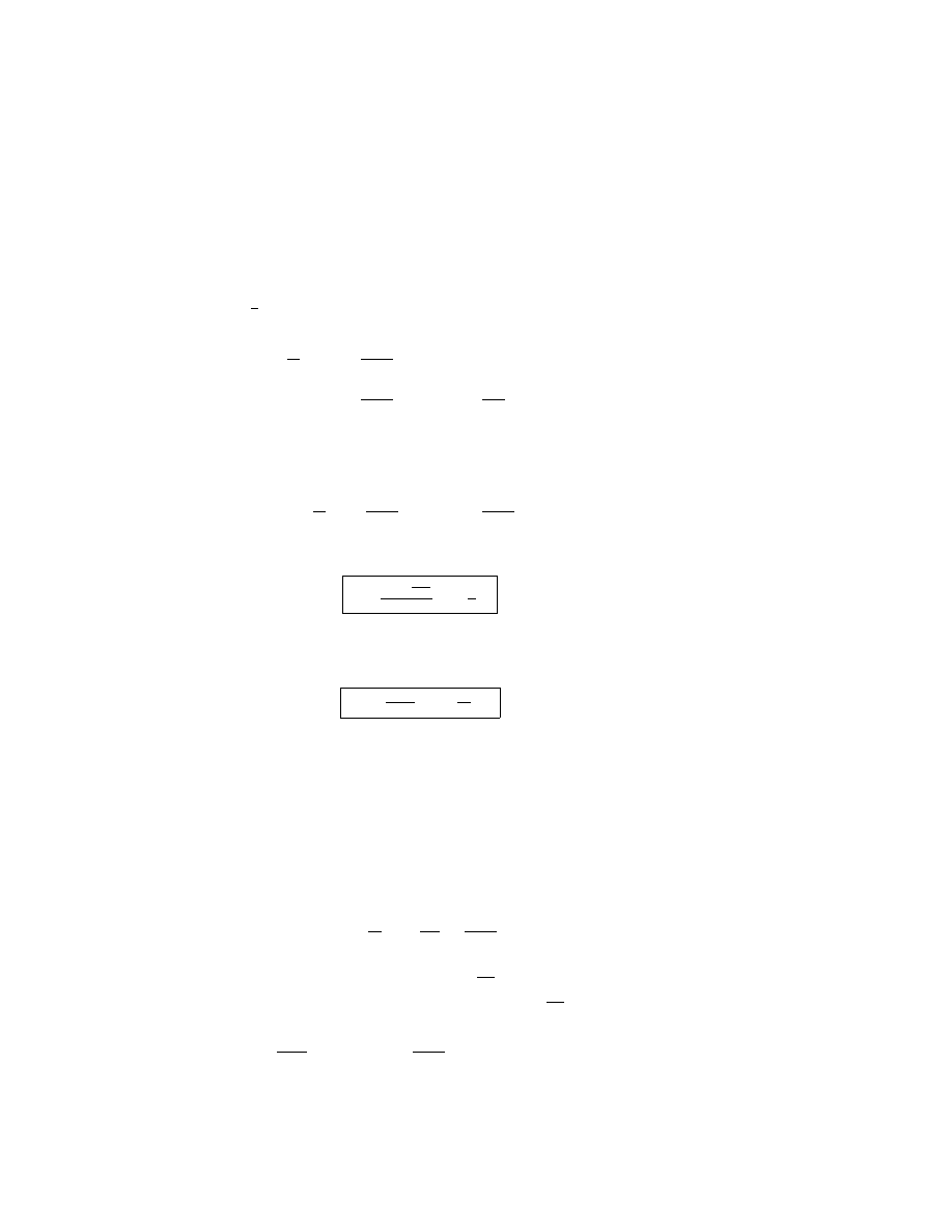
4.7. COSMOLOGY WITH THE SCALAR FIELD

still obtaining

ρ + ρ

= ˜

ρ + ˜

= ¯

ρ + ¯

(4.178)

Assuming p =

ρ we have (compare to equation 4.171)

−qH

≡

−

4πG

[(1 + γ)ρ

− 2ρ

]

−

4πG

[(1 + γ

− m

) ¯

ρ + (m

− 2)¯ρ

]

(4.179)

(where we have used the second expression in 4.177), which we would like
to write as

−qH

≡

−

4πG

( ¯

ρ + 3¯

−

4πG

( ¯

+ 3¯

(4.180)

This is achieved if we make the following definitions

≡

−m

ρvo

ρo

≡

(4.181)

and

≡

−3

(4.182)

4.7.11

Quantization

All of our proceeding work with the scalar field was at the classical level. In
this section we wish to consider quantum effects.

In section (2.4.2) we dervied the wheeler-DeWitt equation in minisuper-

space approximation. We began with the Lagrangian in equation (2.20)

L =

−κR

[(

)

−

8πG

(ρ + ρ

)]

(4.183)

and identified the conjugate momentum p

≡

∂L

∂ ˙

−2κ ˙RR and derived the

Wheeler-DeWitt equation, after quantizing with p

→ i

∂

∂R

, as

{−

∂

∂R

+ 4κ

[kR

−

8πG

(ρ + ρ

]

}ψ = 0.

(4.184)

CHAPTER 4. ENERGY-MOMENTUM TENSOR

Notice that our quantization ’didn’t do anything to the density.”

In the work that we have done in the present chapter we have made

an effort to write the scalar field as a function of R, i.e. φ = φ(R) and
using ρ =

1
2

+ V (φ) we have written as an effective density ρ(R) for

the scalar field.

Our intention has been to simply insert this ρ(R) into

the Wheeler-DeWitt equation (4.184). In our work on inflation we found
that for ρ

∝

dominating the Friedmann equation then inflation occurs

for m < 2. If this density also dominates ρ + ρ

in the Wheeler-DeWitt

equation, then a tunnelling potential will only be present for m < 2. Thus
inflation and quantum tunnelling require the same condition. This leads us
to the hypothesis that inflation and quantum tunnelling are identical! Or in
other words, inflation is simply a classical description of quantum tunnelling.
We call this hypothesis Quantum Inflation.

Quantum inflation is easy to validate for ordinary densities, either ρ or

, that behave like ρ

∝

. With our discussion of the scalar field we have

written ρ

∝

so it would seem that the idea of quantum inflation also

works for scalar fields.

In our quantization procedure we ”didn’t do anything to the density.” In

terms of scalar fields then this quantization procedure is different to what
other people do with quantization. The usual procedure [?, ?, ?, 20, 21] is
to quantize φ and R seperately and arrive at a Wheeler- DeWitt equation
in terms of both of these variables. Let us now study this procedure.

We begin with the Lagrangian

L =

−κR

[(

)

−

] + 2π

[

− V (φ)]

(4.185)

where κ

≡

3π

From this one can deduce that

(

)

8πG

(

+ V )

−

(4.186)

and also

φ + 3H ˙

φ + V

= 0

(4.187)

provided one uses

R
R

−

4πG

(ρ + 3p) with ρ =

1
2

+ V and p =

1
2

− V .

(NNN see FE)

The canonical momenta are

≡

∂L

∂ ˙

−2κR ˙R

(4.188)

4.7. COSMOLOGY WITH THE SCALAR FIELD

and

≡

∂L

∂ ˙

= 2π

φ.

(4.189)

The Hamiltonian (H = p

− L) becomes (using κ =

3π

)

R + Π

− L

(4.190)

−κR

[(

)

−

8πG

(

+ V )]

≡ 0

(4.191)

where the result H = 0 is obtained by comparing the expression for the
Hamiltonian to the Friedmann equation (4.186). This Hamiltonian is exactly
analogous to the Hamiltonian we had in equation (2.22) where we had ρ
instead of

1
2

+ V .

Writing H in terms of the conjugate momenta we have

H =

−κR

[

4κ

−

8πG

(

2
φ

8π

+ V )] = 0

(4.192)

which, of course is also equal to zero. This Hamiltonian is inherited to
equation (11.34), Pg.462 of the book by Kolb and Turner [21]. This equation
is re-arranged as

2
R

−

4πG

2
φ

9π

(kR

−

8πG

V R

) = 0.

(4.193)

In order to compare to our signal Wheeler-DeWitt equation let’s replace Π

with Π

= 2π

φ, which results in

2
R

9π

[kR

−

8πG

(

+ V )R

] = 0

(4.194)

which is exactly analogous to our original Wheeler-DeWitt equation (2.24)
where we had ρ instead of

1
2

+ V .

Equation (4.193) is quantized by making the replacements

→ −i

∂

∂R

(4.195)

and

→ −i

∂

∂φ

(4.196)

and setting Hψ = 0 to give

CHAPTER 4. ENERGY-MOMENTUM TENSOR

[

−

∂

∂R

4πG

∂

∂φ

9π

(kR

−

8πG

)]ψ = 0

(4.197)

which is the Wheeler-DeWitt equation in minisuperspace approximation for
a quantized scalar field φ. This is identical to equation (10.1.11), Pg.270 of
the book by Linde [36].

We identify the potential as

U (R, φ) =

9π

(kR

−

8πG

V R

)

(4.198)

which is identical to equation (11.35), Pg.463 of the book by Kolb and Turner
[21]. In equation (10.1.25), Pg277 of the book by Linde [36], he gives an
expression for V (R, φ) =

3π

V (a), so that our result does agree with Linde.

We can see that the above method of quantizing the scalar field φ directly

is still consistent with our idea of Quantum Inflation.

Recall that ρ(R)

and V (R) in terms of φ(R) obvioulsy ρ, V and ˙

must have the same R

dependence. Thus if ρ

∝

then also V

∝

in the same way. Thus our

potential U (R, φ) will alsways exhibit a tunnelling shape for m < 2. Thus
Quantum Inflation still works for U (R, φ) when φ is quantized seperately.

4.8

Problems

4.1 Show that ∂

= 0 is the equation of continuity

∂ρ

∂t

∇ · j = 0 where

≡ (ρ, j).

4.2 Show that the above equation of continuity also results from taking the
divergence of Amp`

er´

es law.

4.3 Show that the Lagrangian in equation (4.49) yields the equation of mo-
tion (4.50).

4.4 A) Solve the differential equation (4.56).

B) Check your answer by

substituting your solution back into the equation.

4.5 Now put your solution from problem 4.4 into the Friedmann equation
(4.53) and solve for R(t).

4.8. PROBLEMS

4.6 A) If (

R
R

)

∝

, show that R

∝ t

2/m

. B) If H

≡ (

R
R

)

= constant

show that R

∝ e

4.7 If (

R
R

)

8πG

, show that R = R

8πG

−t

)

4.8 Show that inflationary solutions are characterized by ¨

R > 0 and non-

inflationary expansions by ¨

R < 0

4.9 Barrow’s model is V (φ)

≡ βe

−λφ

. Check that φ(t) =

√

2A ln t is a

soluttion and evaluate the constants β and λ in terms of A.

4.10 Prove equations (4.103)-(4.108).

CHAPTER 4. ENERGY-MOMENTUM TENSOR

Chapter 5

EINSTEIN FIELD
EQUATIONS

The Einstein’s field equations are

µν

= 8πGT

µν

+ Λg

µν

(5.1)

which are a set of 16 coupled equations which will give g

µν

(buried inside

µν

) gives T

µν

. Actually there are only 10 independent equations because

of the symmetry g

µν

= g

νµ

In principle our job is easy. Just write down T

µν

and solve for g

µν

which

specifies the metric. Then we can calculate the paths of light rays, the orbits
of planets, etc. In practice the solution of the Einstein field equations are
exceedingly difficult and only a few exact solutions are known.

Two excellent reference for this section are Chapter 7 of the book by

Lawden [?] and Chapter 2 of the book by Islam [13].

In actual practice, the way one usually solves the Einstein’s equations

is to specify a metric in general terms which contains unknown coefficients.
This metric is substituted into the Einstein equations and one solves for the
unknown coefficients.

Thus we need to learn how to derive the metric for the spaces un-

der consideration. Let us learn how to derive the Friedmann-Robertson-
Walker (FRW) metric which is the metric appropriate to a homogeneous
and isotropic universe but where size can change with time.

CHAPTER 5. EINSTEIN FIELD EQUATIONS

5.1

Preview of Riemannian Geometry

5.1.1

Polar Coordinate

A general N-dimensional Riemannian space, denoted by

, is one in which

the distance ds between two neighboring points can be written (Pg. 88 [?])

= g

µν

(5.2)

If coordinates can be found such that

= dx

(5.3)

over the whole space then the space is said to be Euclidean and is denoted
by

. Clearly

is a special case of

Below we shall restrict our discussion to the spatial part of the metric

denoted as

= h

(5.4)

We shall very often have (eg. FRW and special relativity metrics)

= c

− d`

(5.5)

so that

−g

(5.6)

Consider the two dimensional space where

= dr

+ r

dθ

(5.7)

Here h

= 1, h

= h

= 0, h

= r

. The space looks like

but actually it

because we can find coordinate such that (5.3) is true. These coordinate

are the two-dimensional plane polar coordinates

r cos θ

(5.8)

r sin θ

(5.9)

in which

= dx

+ dy

(5.10)

with g

= g

=1 and g

= g

= 0 or g

µν

= δ

µν

5.1. PREVIEW OF RIEMANNIAN GEOMETRY

Recall that for 3-dimensional spherical polar coordinates

r sin θ cos φ

(5.11)

r sin θ sin φ

(5.12)

r cos θ

(5.13)

and the increments of length d`

, d`

is the e

, e

and e

directions

respectively are

(5.14)

rdθ

(5.15)

r sin θdφ.

(5.16)

Thus the surfaces of a sphere is an example of a space which is

and

cannot be reduced to

. On the surface of the sphere the distance between

two points is

2
θ

+ d`

2
φ

(5.17)

dθ

+ r

sin

θdφ

(5.18)

where h

= r

, h

= h

= 0, h

= r

sin

θ. For this surface it is not

possible to find x, y such that ds

= dx

+ dy

and therefore the surface of

a sphere is not

∈

but rather a genuine

∈

space.

5.1.2

Volumes and Change of Coordinates

The measure is the volume element in some set of coordinates. There are 3
ways to calculate the measure.

1) Infinitesimal Length Method is one in which one identifies the infin-

tesimal increments of length and simply multiplies them together to get the
volume element. In Cartesian Coordinates we have d`

= dx, d`

= dy, and

= dz to give

dV = d`

= dxdydz.

(5.19)

In 2-d plane polar coordinates d`

= dr and d`

= rdθ to give

dV = d`

= rdrdθ

(5.20)

(actually this ”volume” is an area). In 3-D spherical polar coordinates d`

dr, d`

= dθ and d`

= r sin dφ to give

dV = d`

= r

sin θdrdθdφ.

(5.21)

CHAPTER 5. EINSTEIN FIELD EQUATIONS

2) Jacobian Method is the one usually mentioned in introductory calculus

books ([?] Pg.746) for changing variables. Suppose x = x(u, v) and y =
y(u, v) then

Z Z

f (x, y)dxdy =

Z Z

f [x(u, v), y(u, v)]

| J(u, v) | dudv

(5.22)

where

| J(u, v) | is the modulus of the Jacobian defined as

J (u, v)

≡

¯¯

∂x
∂u

∂x
∂v

∂y
∂u

∂y
∂v

¯¯

(5.23)

For 3-dimensions with x = x(u, v, w), y = y(u, v, w) and z = z(u, v, w) we
have

J (u, v, w)

≡

¯¯

∂x
∂u

∂x
∂v

∂x

∂w

∂y
∂u

∂y
∂v

∂y

∂w

∂z

∂u

∂z
∂v

∂z

∂w

¯¯

(5.24)

For Cartesian coordinates obviously J (x, y, z) = 1. For plane polar coordi-
nates (x = r cos θ, y = r sin θ)

J (r, θ) =

¯¯

cos θ

−r sin θ

sin θ

r cos θ

¯¯

= r

(5.25)

and for spherical polar coordinates (x = r sin θ cos φ, y = r sin θ cos φ, z =
r cos θ)

J (r, θ, φ) =

¯¯

sin θ cos φ

r cos θ cos φ

−r sin θ sin φ

sin θ sin φ

r cos θ sin φ

r sin θ cos φ

cos θ

−r sin θ

¯¯

= r

sin θ

(5.26)

The volume element in 2-d is

dV =

| J(u, v) | dudv

(5.27)

and in 3-d it is

dV =

| J(u, v, w) | dudvdw

(5.28)

which then reproduce equations (5.19), (5.139) and (5.140) for Cartesian,
plane polar and spherical polar coordinates.

3) Metric Tensor Method is what we prefer in general relativity. Here

([21], Pg.33)

5.1. PREVIEW OF RIEMANNIAN GEOMETRY

dV =

√

hdudvdw

(5.29)

where h is the determinant of the spatial metric tensor. Thus

| J |=

√

(5.30)

For a plane polar coordinates ds

= dr

+ r

dθ

≡ g

so that

h =

¯¯

= r

(5.31)

giving

√

h = r so that dV =

√

hdrdθ in agreement with (5.139). For spherical

polar coordinates d`

= dr

+ r

dθ

+ r

sin

θdφ

≡ h

giving

h =

¯¯

sin

¯¯

= r

sin

(5.32)

giving

√

h = r

sin θ so that dV =

√

hdrdθdφ = r

sin θdrdθdφ in agreement

with (5.140).

Thus define

≡ dudv

≡ dudvdw

≡ dudvdwdt

(5.33)

so that the measure is

dV =

√

x or

√

(5.34)

depending on the number of dimensions. It is important to remember that
d

x or d

x om this notation is not d`

or d`

but simply only

the coordinates. For example in spherical polar coordinates

≡ drdθdφ

(5.35)

or with time

≡ drdθdφdt.

(5.36)

The measure is volume is obtained with dV =

√

x or

√

−gd

x (because

for 4-d we use g

µν

and h

−g

and h =

−g). Thus in general

CHAPTER 5. EINSTEIN FIELD EQUATIONS

6= d

in contrast to conventions used, say in undergraduate physics books.

5.1.3

Differential Geometry

A Good reference for differential geometry is the book by Lipschutz [?].
Introductory material is discussed by Purcell and Varberg [?] (Pg.625-634,
285-290).

Previously we wrote the definition of a circle as x

+ y

= r

which

could be written generally as y = y(x). The same equation can be expressed
parametrically in terms of the parameter θ as x = r cos θ and y = r sin θ or
generally as x = x(θ) and y = y(θ). For many curves the form y = y(x)
can be clumsy and nowadays mathematicians always prefer the parametric
representation. (See [?] Pg.570). Another way to write our equation for the
circle (radius=1) is

x = cos θˆ

+ sin θˆ

(5.37)

where ˆ

and ˆ

are basis vectors in

Thus a general curve (Chapter 3 of [?]) is expressed as

x = x(t)

(5.38)

where t is the parameter. If the basis is chosen to be

then x = x(t) is

equivalent to two scalar equations x

= x

(t) and x

= x

(t). Thus a curve

can be specified in any number of dimensions. For our circle above we have
x

= x

(θ) = cos θ and x

= x

= sin θ.

A general surface (Chapter 8 of [?]) is expressed as

x = x(u, v).

(5.39)

If, for example, the basis in

then

x(u, v) = x

(u, v)ˆ

+ x

(u, v)ˆ

+ x

(u, v)ˆ

(5.40)

Good references of the next 3 sections are the books by Kolb and Turner

([21], Pg.31-35) and Landau ([?], Pg.177-181) and Ohanian and Ruffini ([8],
Pg546-552) and Chow ([28], Pg.197-200) and the article by Kung [?].

5.1. PREVIEW OF RIEMANNIAN GEOMETRY

5.1.4

1-dimesional Curve

Let us first consider the circle, often called the one sphere denoted by S

Recall that for a circle the radius R, the proper way to express it is in terms
of 1-dimensional parameter θ as

x(θ) = R(cos θˆ

+ sin θˆ

(5.41)

However in introductory books one always introduces a ficticous extra di-
mension and embeds the 1-d curve in a 2-d Euclidean space via

+ y

= R

(5.42)

which we recognize as the equation for a circle. Remember though this
equation is really overkill. It is a 2-d equation for a 1-d curve! The 1-
parameter equation (5.41) is much better. We can also write

2
1

+ x

2
2

= R

(5.43)

The element of length in the 2-d Euclidean space is

= dx

2
1

+ dx

2
2

(5.44)

In an ordinary 2-d Euclidean space x and y (or x

and x

) are free to vary

independently and this is how the whole 2-d space get covered. Equation
(5.44) is true in general. However the reason that (5.42) or (5.43) describes
a circle is because it constrains the value of y in terms of x. This constraint
(5.42) picks our only those points in

which give the circle.

Equation (5.44) covers all of

. We can constrain it for the circle by

reducing the two parameters x

and x

to only one parameter. Thus we will

have d` for the circle. We do this using the 2-d constraint (5.43) and writing
y =

√

− x

and dy =

−x

√

−x

dx so that

− x

(5.45)

Note that dy

≡ (dy)

and dy

6= d(y

). Thus (5.44) becomes

− x

(5.46)

CHAPTER 5. EINSTEIN FIELD EQUATIONS

This can also be written in terms of the dimensionless coordinate

≡

(5.47)

to give

= R

− r

(5.48)

where R is the radius of the space (the circle).

Another convenient coordinate system for the circle use the angle θ from

plane polar coordinates specified via

R cos θ

R sin θ.

(5.49)

Identifying the increments of length d`

and d`

in the ˆ

and ˆ

directions

Rdθ

(5.50)

then

2
R

+ d`

2
θ

+ R

dθ

(5.51)

which gives the distance d` in the 2-d space. To restrict ourselves to the rim
of the circle (curved 1-d space) we fix d`

= dR = 0 and get

= R

dθ

(5.52)

which makes it obvious that the space is the one sphere (circle) of radius R.
Using simple trigonometry one can show that (5.52) is the same as (5.46).
(Do Problem 5.1)

Using d`

≡ h

we evidently have

= (R

)

(5.53)

which is a 1-dimensional ”motion”. The determinant is obviously h = R

giving

√

h = R. This allows us to calculate the volume (we are calling the

length a geological volume) as

V =

√

x =

2π

Rdθ = 2πR

(5.54)

5.1. PREVIEW OF RIEMANNIAN GEOMETRY

The 1-d curve that we described above is the circle or one sphere denoted

. However there are three 1-d spaces which are homogeneous and isotropic.

There are i) the flat x line (R

), ii) the positively curved one sphere (S

)

derived above and iii) the negatively curved hyperbolic curve (H

). [21]

The formulas for a space of constant negative curvature [21] can be ob-

tained with the replacement

→ iR

(5.55)

to yield

−R

− x

+ x

(5.56)

or using r

≡

= R

1 + r

(5.57)

These results are also obtained by embedding in Minkowski space ( do Prob-
lem 5.2).

The line element for a space of zero curvature is obviously just

= dx

(5.58)

or using r

≡

= R

(5.59)

These formulas are obtained from S

or H

by letting R

→ ∞.

We can collect our results for R

, S

and H

into a single formula

− kx

(5.60)

or using r

≡

= R

−kR

(5.61)

where k = 0, +1,

−1 for flat, closed and open curves respectively. (i.e. for

, S

and H

respectively)

CHAPTER 5. EINSTEIN FIELD EQUATIONS

5.1.5

2-dimensional Surface

Kolb and Turner [21] analyze this problem very nicely. Other references are
listed following equation (5.40).

A surface is represented by two parameters u, v and expressed as x =

x(u, v) as mentioned previously. However we shall introduce a surface ficti-
cious coordinate (three parameters) and embedding the surface in

. Thus

with 3 parameters the equation for the two sphere is

+ y

+ z

+ R

(5.62)

which we recognize as the equation for a sphere used in introductory books.
However this equation is overkill. It is a 3-d equation for a 2-d surface. We
can also write

2
1

+ x

2
2

+ x

2
3

= R

(5.63)

Any 3-d Euclidean space

has length element

= dx

2
1

+ dx

2
2

+ dx

2
3

(5.64)

which under normal circumstances would map out the whole 3-d volume.
However (5.63) restricts x

according to

2
3

= R

− x

2
1

− x

2
2

(5.65)

Writing

∂x

(5.66)

and with

∂x

−x

√

−x

2
1

−x

2
2

we have

−

+ x

− x

(5.67)

2
3

+ x

)

− x

(5.68)

to give ([21], Pg.32)

= dx

2
1

+ dx

2
2

+ x

)

− x

(5.69)

5.1. PREVIEW OF RIEMANNIAN GEOMETRY

which is re-written as

− x

[(R

−x

2
2

)dx

2
1

+(R

−x

2
1

)dx

2
2

(5.70)

Let us introduce plane polar coordinates in the x

plane as

= r

cos θ

= r

sin θ.

(5.71)

These coordinates are shown very clearly in Fig 2.1, Pg.32 of Kolb and

Turner [21]. Thus

→ 2π

→ R.

(5.72)

Using

∂x

∂θ

dθ

(5.73)

then (5.69) and (5.70) become

− r

+ r

dθ

(5.74)

This can also be written in terms of the dimensionless coordinate

≡

(5.75)

to give

= R

[

− r

+ r

dθ

]

(5.76)

where

r : 0

→ 1.

(5.77)

Another convenient coordinate system for the two sphere uses angles θ

and φ from spherical polar coordinates specified via

R sin θ cos φ

(5.78)

R sin θ sin φ

(5.79)

R cos θ

(5.80)

and substituting into (5.64) directly yields

= R

(dθ

+ sin

θdφ

(5.81)

CHAPTER 5. EINSTEIN FIELD EQUATIONS

Equation (5.81) is alternatively obtained by identifying the increments of
length d`

, d`

in the ˆ

, ˆ

and ˆ

directions as

(5.82)

Rdθ

(5.83)

R sin θdφ

(5.84)

then

2
R

+ d`

2
θ

+ d`

2
φ

+ R

(dθ

+ sin

θdφ

)

(5.85)

gives the distance ds in the 3-d space. To restrict ourselves to the surface of
the sphere (curved 2-d space) we find d`

= dR = 0 and get

= R

(dθ

+ sin

θdφ

)

(5.86)

in agreement with (5.81).

Using d`

≡ h

we evidently have for S

sin

(5.87)

The determinant is obviously

h = R

sin

(5.88)

giving

√

h = R

sin θ. The volume (we are calling the surface area a gener-

alized volume) is

V =

√

x =

√

hdθdφ + R

sin theta

2π

dφ = 4πR

(5.89)

Actually there are three 2-d spaces which are homogenous and isotropic.

There are 1) the flat x

− y plane (R

), ii) the positively curved two sphere

) and iii) the negatively curved two hyperbola (H

As before we can obtain the formula for H

with the replacement

→ iR

(5.90)

to yield

= R

[

1 + r

+ r

dθ

(5.91)

5.1. PREVIEW OF RIEMANNIAN GEOMETRY

This result is also obtained by embedding in Minkowski space. The metric
corresponding to (5.81) is ([21], Pg.34, equation 2.17)

= R

(dθ

+ sin

θdφ

(5.92)

We can collect our results for R

, S

and H

into a single formula

= R

(

− kr

+ r

dθ

)

(5.93)

where k=0, +1, -1 for flat (R

), closed (S

) and open (H

) surfaces respec-

tively.

The volume can be alternatively calculated using d`

= h

(5.93) we have

−kr

(5.94)

giving the determinant

h =

− kr

(5.95)

√

h =

√

−kr

. The volume is

√

x =

√

h = R

rdr

√

− kr

2π

dθ

(5.96)

2πR

rdr

√

− kr

(5.97)

The limits of integration

dr can be clearly seen from Fig 2.1 of Kolb and

Turner [21], Pg.32. What this really means is

≡ 2

(5.98)

where r = 0 at θ = 0 and r = R at θ =

and r = 0 again at θ = π.

(See bottom Pg.179 and top pg.180 of the book by Lawden [?] for more
explanation)

The integral and its limits are more clearly done with the substitution

√

≡ sin χ

(5.99)

CHAPTER 5. EINSTEIN FIELD EQUATIONS

when

χ : 0

→ π.

(5.100)

Thus

dχ is equivalent to

dr = 2

dr. Thus the volume in equation

(5.97) becomes

V = 2πR

√

sin χdχ

(5.101)

giving

V =

4πR

(5.102)

Thus for k = +1 we have V = 4πR

as before. For k = 0 we have V =

∞

and for k =

−1 we need to do the integral again. We would find V = ∞ for

k =

−1.

5.1.6

3-dimensional Hypersurface

Proceeding upwards in our number of dimensions we might inquire a ”curved
volume”. But the curvature can really only be imagined with respect to
embedding in a 4-dimensional Euclidean space

. We call the 4-d space as

a hypersurface.

Our 4-d Euclidean space (into which we will embed the hypersurface)

has length element

= dx

2
1

+ dx

2
2

+ dx

2
3

+ dx

2
4

(5.103)

(it is d`

and not ds

A hypersurface is represented by three parameters u, v, w and is ex-

pressed as x = x(u, v, w). Introduce an extra ficticious coordinate for the
three sphere S

+ y

+ z

+ w

2
1

+ x

2
2

+ x

2
3

+ x

2
4

(5.104)

which restricts x

2
4

= R

− x

2
1

− x

2
2

− x

2
3

(5.105)

Writing

∂x

(5.106)

5.1. PREVIEW OF RIEMANNIAN GEOMETRY

and with

∂x

−x

√

−x

2
1

−x

2
2

−x

2
3

etc. we have

−

+ x

− x

(5.107)

2
4

+ x

)

− x

(5.108)

to give ([21], Pg.34)

= dx

2
1

+ dx

2
2

+ dx

2
3

+ x

)

− x

(5.109)

Let us introduce spherical polar coordinates in the x

hyperplane as

sin θ cos φ

(5.110)

sin θ sin φ

(5.111)

cos θ

(5.112)

where

→ π

(5.113)

→ 2π

(5.114)

→ R.

(5.115)

Using

∂x

∂r

. +

∂x

∂θ

dθ +

∂x

∂φ

dφ

(5.116)

then (5.109) becomes

− r

+ r

dθ

+ r

sin

θdφ

(5.117)

Introducing the dimensionless coordinate

≡

(5.118)

gives

= R

[

− r

+ r

dθ

+ r

sin

θdφ

]

(5.119)

CHAPTER 5. EINSTEIN FIELD EQUATIONS

where

r : 0

→ 1.

(5.120)

Another convenient coordinate system for the three sphere uses angles

χ, θ, φ from 4-dimensional hyperspherical polar coordinates specified via

R sin χ sin θ cos φ

(5.121)

R sin χ sin θ sin φ

(5.122)

R sin χ cos θ

(5.123)

R cos χ.

(5.124)

Substituting into (5.119) directly yields

= R

[dχ

+ sin

χ(dθ

+ sin

θdφ

)].

(5.125)

Using d`

= h

we have






sin

χ sin






(5.126)

The determinant is

h = R

sin

χ sin

(5.127)

giving

√

h = R

sin

χ sin θ. The volume is

√

x =

√

hdχdθdφ

sin

χdχ

sin θdθ

2π

dφ

(5.128)

where the limits

dχ are the same as in the previous section. Thus

V = 4πR

sin

χdχ = 4πR

[

−

sin 2χ

]

π
0

(5.129)

giving

V = 2π

(5.130)

for the volume of our hypersphere. Compare this to the volume of a Eu-
clidean sphere

4
3

πR

For a flat, open and closed hyperspheres the metric is

= R

[

− kr

+ r

dθ

+ r

sin

θdφ

]

(5.131)

5.2. FRIEDMANN-ROBERTSON-WALKER METRIC

The volume can be calculated alternatively. Using d` = h

(5.131) we have






−kr

sin






(5.132)

giving the determinant h =

sin

−kr

. The volume is

V =

√

hdrdθdφ

√

− kr

sin θdθ

2π

dφ

4πR

√

− kr

(5.133)

The limits of integration are the same as discussed in equation (5.98).

Using the substitution

√

≡ sin χ

(5.134)

with

: 0

→ π

(5.135)

becuase χ : 0

→ π. Thus the volume is

V = 4πR

3/2

sin

χdχ

(5.136)

giving

V =

2π

3/2

(5.137)

For k = +1 this agrees with our result before.

5.2

Friedmann-Robertson-Walker Metric

The metric of Special Relativity is

= c

− (dx

(5.138)

Clearly the spatial part is a 3-d Euclidean flat space. We have seen that the
spatial metric for a homogeneous, isotropic curved space with a size R(t)
that can change in time is

= R

(t)[

− kr

+ r

(dθ

+ sin

θdφ

)].

(5.139)

100

CHAPTER 5. EINSTEIN FIELD EQUATIONS

Replacing the spatial part of the special relativity metric with (5.139) we
have the Friedmann-Robertson-Walker (FRW) metric [13]

= c

− R

(t)[

− kr

+ r

(dθ

+ sin

θdφ

)]

(5.140)

where R(t) is called the scale factor and the constant k can be 0,

±1 depend-

ing on the curvature. This can also be derived with the use of Killing vectors
[13].

Writing ds

≡ g

µν

and identifying

= ct

(5.141)

= r

(5.142)

= θ

(5.143)

= φ

(5.144)

we have

= 1

(5.145)

−R

− kr

(5.146)

−R

(5.147)

−R

sin

(5.148)

Defining the determinant

≡ detg

µν

= g

(5.149)

−

sin

− kr

(5.150)

(Note that this is not g = detg

µν

.) Thus

√

−g =

sin θ

√

− kr

(5.151)

If g

µν

is represented by a matrix [g

µν

], then we found previously that

µν

is just the inverse of this metric namely [g

µν

]

−1

. For a diagonal matrix

(which we have for the FRW metric) each matrix element is simply given by
g

µν

. Thus it’s easy to get

= 1

(5.152)

5.2. FRIEDMANN-ROBERTSON-WALKER METRIC

101

−

− kr

)

(5.153)

−1

(5.154)

−1

sin

(5.155)

5.2.1

Christoffel Symbols

We now calculate the Christoffel symbols using equation (3.69). Fortunately
we need not calculate all of them. We can use the symmetry Γ

α
βγ

= Γ

α
γβ

shorten the job. We have

α
βγ

≡

α²

²β,γ

+ g

αγ,β

− g

βγ,²

) = Γ

α
γβ

αα

αβ,γ

+ g

αγ,β

− g

βγ,α

)

(5.156)

which follows because g

α²

= 0 unless ² = α. (g

µν

is a diagonal matrix for

the FRW metric.) The only non-zero Christoffel symbols are the following:

0
11

01,1

+ g

01,1

− g

11,0

) =

−

11,0

because g

= 0 and g

= 1. This becomes (let’s now set c

≡ 1)

0
11

−

11,0

−

∂

∂t

(

−R

− kr

)

− kr

∂R

∂t

2R ˙

2(1

− kr

)

R ˙

− kr

(5.157)

because r

6= r(t) and R = R(t). Proceeding

0
22

−

22,0

−

∂

∂t

(

−R

) = r

R ˙

(5.158)

0
33

= r

sin

θR ˙

(5.159)

1
11

− kr

(5.160)

1
22

−r(1 − kr

)

(5.161)

1
33

−r(1 − kr

) sin

(5.162)

102

CHAPTER 5. EINSTEIN FIELD EQUATIONS

2
12

= Γ

3
13

(5.163)

2
33

− sin θ cos θ

(5.164)

3
23

= cot θ

(5.165)

1
01

= Γ

2
02

= Γ

3
03

(5.166)

(do Problems 5.2 and 5.3)

5.2.2

Ricci Tensor

Using equation (??) we can now calculate the Ricci tensor. For the FRW
metric it turns out that R

µν

= 0 for µ

6= ν, so that the non-zero components

are R

, R

. Proceeding we have

√

−g

(Γ

²
00

√

−g), −(ln

√

−g)

,00

− Γ

²
0θ

θ
0²

but Γ

= 0 giving

−(ln

√

−g)

,00

− Γ

0
0θ

θ
00

− Γ

1
0θ

θ
01

− Γ

2
0θ

θ
02

− Γ

3
0θ

θ
03

when we have performed the sum over ². The term Γ

θ
0θ

= 0. In the last

three terms we have Γ

α
0θ

where α = 1, 2, 3. Now Γ

α
0θ

= 0 for θ

6= α, so that

we must have θ = 1, 2, 3 in the third, forth and fifth terms respectively. Also
the second term contains Γ

0
0θ

which is always 0. Thus

−(ln

√

−g)

,00

− Γ

1
10

1
01

− Γ

2
02

− Γ

3
03

−(ln

√

−g)

,00

− (Γ

1
01

)

− (Γ

2
02

)

− (Γ

3
03

)

−(ln

√

−g)

,00

− 3(

)

Now

(

√

−g)

∂

√

−g

∂x

∂

√

−g

∂t

sin θ

√

− kr

∂R

∂t

sin θ

√

− kr

and

(ln

√

−g)

,µ

≡

∂ ln

√

−g

∂x

∂ ln

√

−g

∂

√

−g

∂

√

−g

∂x

√

−g

∂

√

−g

∂x

5.2. FRIEDMANN-ROBERTSON-WALKER METRIC

103

so that

(ln

√

−g)

−

√

−g

∂

√

−g

∂x

√

− kr

sin θ

√

− kr

R = 3

giving

(ln

√

−g)

,00

= 3

∂

∂t

(

) = 3

R ¨

− ˙R

= 3

− 3(

)

We finally have

−3

(5.167)

One can similaraly show that

R ¨

− 2 ˙R

+ 2k

− kr

(5.168)

= r

(R ¨

R + 2 ˙

+ 2k)

(5.169)

= r

sin

θ(R ˙

R + 2 ˙

+ 2k)

(5.170)

(do Problem 5.4)

5.2.3

Riemann Scalar and Einstein Tensor

We now calculate the Ricci scalar

R≡ RR

≡ g

αβ

. The only non-zero

contributions are

R = g

+ g

(5.171)

−6[

+ (

)

]

(5.172)

(do Problem 5.5). Finally we calculate the Einstein tensor G

µν

≡ R

µν

−

1
2

µν

. The only non-zero component are for µ = ν. We obtain

= 3[(

)

]

(5.173)

−1

− kr

(2 ¨

RR + ˙

+ k)

(5.174)

−r

(2 ¨

RR + ˙

+ k)

(5.175)

−r

sin

θ(2 ¨

RR + ˙

+ k)

(5.176)

(do Problem 5.6).

104

CHAPTER 5. EINSTEIN FIELD EQUATIONS

5.2.4

Energy-Momentum Tensor

For a perfect fluid the energy momentum tensor is given in equation (4.26)
as

µν

= (ρ + p)u

µν

− pη

µν

(5.177)

The tensor for T

µν

is written is (4.28) for the metric of Special Relativity.

For an arbitrary metric in General Relativity we have

µν

= (ρ + p)u

µν

− pg

µν

(5.178)

where we shall use g

µν

from our FRW model. For a motionless fluid recall

that u

= (c, 0) or U

= (c,

−0) = (c, 0) = (1, 0) for c ≡ 1. Thus

= ρ + p

− p = ρ

(5.179)

and

−pg

(5.180)

because u

= 0. Upon substitution of the FRW values for the metric given

is equations (5.145)-(5.148) we have

µν








−kr

sin








(5.181)

5.2.5

Friedmann Equations

Finally we substitute our results into the Einstein field equations G

µν

8πGT

µν

+ Λg

µν

The µν = 00 component is

3[(

)

] = 8πGρ + Λ

giving

≡ (

)

8πG

−

(5.182)

The µν = 11 component is

−1

− kr

(2 ¨

RR + ˙

+ k) = 8πGp

− kr

+ Λ

−R

− kr

5.3. PROBLEMS

105

giving

+ (

)

−8πGp + Λ.

But we now use our previous result (5.182) to give

8πG

ρ +

−8πGp + Λ

to finally give

4πG

(ρ + 3p) +

(5.183)

(do Problem 5.7).

5.3

Problems

5.1 For the FRW metric show that Γ

− (1 − kr

)r sin

θ and Γ = cot θ.

5.2 Show that, for example, Γ

= Γ

= 0 for the FRW metric.

5.3 Show that R

= r

(R ¨

R + 2 cot R

+ 2k) for the FRW metric.

5.4 Show that the Ricci scalar is

R= −6[

R
R

+ (

R
R

)

] for the FRW metric.

5.5 Calculate G

µν

for the FRW metric.

5.6 Show that the µν = 22 and µν = 33 components of the Einstein’s
equations for the FRW metric yield the same equation (5.63) as the µν = 11
component.

106

CHAPTER 5. EINSTEIN FIELD EQUATIONS

Chapter 6

Einstein Field Equations

µν

= kT

µν

go through history e.g. he first tried R

µν

= kT

µν

etc

107

108

CHAPTER 6. EINSTEIN FIELD EQUATIONS

Chapter 7

Weak Field Limit

derivation of G

µν

= kT

µν

from equiv princ.

109

110

CHAPTER 7. WEAK FIELD LIMIT

Chapter 8

Lagrangian Methods

Lagrangians for G

µν

etc.

(NNNN have assumed special relativity g

= +1) (NNN

5φ term seems

to disagree with Kolb and Turner Pg. 276 eqn 8.20).

111

112

CHAPTER 8. LAGRANGIAN METHODS

Bibliography

[1] J.B. Marion, Classical Dynamics of Particles and Systems, 3rd ed.,

(Harcourt, Brace, Jovanovich College Publishers, New York, 1988).
QA845 .M38

[2] J.Foster and J.D Nightingale, A Short Course in General Relativity,

2nd ed., (Springer-Verlag, 1995). QC173.6 .F67

[3] S. Gasiorowicz, Quantum Physics, (Wiley, New York, 1996).

[4] H.A. Atwater, Introduction to General Relativity, (Pergamon, New

York, 1974).

[5] B.F. Schutz, A First Course in General Relativity, (Cambridge Univer-

sity Press, New York, 1990). QC173.6.S38

[6] B.F. Schutz, Geometrical methods of mathematical physics, (Cambridge

University Press, New York, 1980). QC20.7.D52

[7] J.V. Narlikar, Introduction to cosmology, 2nd ed., (Cambridge Univer-

sity Press, New York, 1993). QB981.N3

[8] H. Ohanian and R. Ruffini, A Gravitation and Spacetime, 2nd ed.,

(W.W. Norton and Company, New York, 1994). QC178 .O35

[9] J.L. Martin, General Relativity, (Ellis Horwood Limited, Chichester,

England, 1988).

[10] A. Guth and P. Steinhardt, The Inflationary Universe, in The New

Physics, edited by P. Davies, (Cambridge University Press, New York,
1989).

[11] D. Atkatz, American J. Phys. 62, 619 (1994).

113

114

BIBLIOGRAPHY

[12] R. Kubo, Statistical Mechanics, (North-Holland, Amsterdam, 1967).

[13] J.N. Islam, An Introduction to Mathematical Cosmology, (Cambridge

University Press, New York, 1992).

[14] H.A. Atwater, Introduction to General Relativity, (Pergamon, New

York, 1974).

[15] R. Adler, M. Bazin, M. Schiffer, Introduction to General Relativity,

(McGraw-Hill, New York, 1975).

[16] T. Jacobson, Phys. Rev. Lett. 75, 1260 (1995)

[17] W. Freedman et al, Nature D 371, 757 (1994).

[18] L.M. Krauss and M.S. Turner, The cosmological constant is back, Gen-

eral Relativity and Gravitation, 27, 1137 (1995).

[19] A. Guth, Phys. Rev. D 23, 347 (1981).

[20] J. Hartle and S. Hawking, Phys. Rev. D 28, 2960 (1983).

[21] E.W. Kolb and M.S. Turner, The Early Universe, (Addison-Wesley,

1990).

[22] D. Atkatz and H. Pagels, Phys. Rev. D 25, 2065 (1982).

[23] F.W. Byron and Fuller, Mathematics of Classical and Quantum Physics,

vols. 1 and 2,
(Addison-Wesley, Reading, Masachusetts, 1969). QC20.B9

[24] G.B. Arfken and H.J. Weber, Mathematical Methods for Physicists, 4th

ed., (Academic Press, San Diego, 1995). QA37.2.A74

[25] H.C. Ohanian, Classical Electrodynamics, (Allyn and Bacon, Boston,

1988). QC631.O43

[26] J.D. Jackson, Classical Electrodynamics, (Wiley, New York, 1975).

QC631.J3

[27] J.B. Marion, Classical Electromagnetic Radiation, (Academic Press,

New York, 1965). QC631.M37

[28] T. L. Chow, General Relativity and Cosmology, (Wuerz Publishing Ltd.,

Winnipeg, Canada, 1994).

BIBLIOGRAPHY

115

[29] M.S. Madsen, The Dynamic Cosmos, (Chapman and Hall, New York,

1995).

[30] H. Muirhead, The physics of elementary particles, (Pergamon Press,

New York, 1965). QC721.M94

[31] M. Leon, Particle physics: an introduction, (Academic Press, New York,

1973). QC793.2.L46

[32] R. D’Inverno, Introducing Einstein’s Relativity, (Clarendon Press, Ox-

ford, 1993).

[33] P.J.E. Peebles, Principles of Physical Cosmology, (Princeton University

Press, Princeton, New Jersey, 1993).

[34] B.D. Serot and J. D. Walecka, The Relativistic Nuclear ManyBody Prob-

lem, Advances in Nuclear Physics, 16, 1 (1986). edited by J.W. Negele
and E. Vogt (Plenum Press, New York, 1986).

[35] J. D. Barrow, Cosmic No-Hair Theorem and Inflation, Physics

Lett. B, 187, 112, (1987)

[36] A. D. Linde, Inflation and Quantum Cosmology, (Academic Press, New

York, 1990)

[37] P. D. B. Collins, A. D. Martin and E. J. Squires, Particle Physics and

Cosmology, (Wiley, New YOrdk, 1987)

[38] A. D. Dolgov, M. V. Sazhin and Y. B. Zeldovich, Basis of Modern

Cosmology (Editions Fronti`

eres, B.P.33, 91192 Gif-Sur-Yvette Cedex,

France, 1990)

Wyszukiwarka

Podobne podstrony:
General Relativity and Quantum Cosmology Madore
Jose Wudka Space Time, Relativity and Cosmology Ch5 The Clouds Gather
Eurocode 2 Part 1 1 2004 NA UK Design of concrete structures General rules and rules for buildin
Norbury Quantum field theory (Wisconsin lecture notes, 2000)(107s)
General Relativity Theory, Quantum Theory of Black Holes and Quantum Cosmology
Introduction to Tensor Calculus for General Relativity
Introduction to Differential Geometry and General Relativity
Eurocode 8 Part 1 1998 2004 Design of Structures for Earthquake Resistance General Rules Seism
Einstein, Special and General Relativity
Introduction to relativistic astrophysics and cosmology through Maple
Tips and improvements for the general occultist
British Patent 2,812 Improvements in Methods of and Apparatus for the Generation of Electric Current
Eurocode 3 Part 1 3 2006 UK NA Design of steel structures General rules Supplementary rules for
British Patent 8,575 Improved Methods of and Apparatus for Generating and Utilizing Electric Energy
Applications and opportunities for ultrasound assisted extraction in the food industry — A review
Law and Practice for Architects
2 grammar and vocabulary for cambridge advanced and proficiency QBWN766O56WP232YJRJWVCMXBEH2RFEASQ2H
VENTILATION AND COOLING IN UNDERGROUND MINES (2)

więcej podobnych podstron