Linear mixed-integer models for biomass supply chains with transport, storage
and processing

Silke van Dyken

, Bjorn H. Bakken, Hans I. Skjelbred

SINTEF Energy Research, Sem Saelands vei 11, NO-7465 Trondheim, Norway

a r t i c l e

i n f o

Article history:
Received 23 February 2009
Received in revised form
17 November 2009
Accepted 18 November 2009
Available online 7 December 2009

Keywords:
Energy supply systems
Biomass
Long-term processes
Linear mixed-integer models

a b s t r a c t

This paper presents a linear mixed-integer modeling approach for basic components in a biomass supply
chain including supply, processing, storage and demand of different types of biomass. The main focus in
the biomass models lies on the representation of the relationship between moisture and energy content
in a discretized framework and on handling of long-term processes like storage with passive drying
effects in the optimization. The biomass models are formulated consistently with current models for gas,
electricity and heat infrastructures in the optimization model ‘eTransport’, which is designed for plan-
ning of energy systems with multiple energy carriers. To keep track of the varying moisture content in
the models and its impact on other biomass properties, the current node structure in eTransport has
been expanded with a special set of biomass nodes. The Node, Supply, Dryer and Storage models are
presented in detail as examples of the approach. A sample case study is included to illustrate the
functionality implemented in the models.

1. Introduction

Biomass can be deﬁned as organic matter that has been directly

or indirectly derived from contemporary photosynthesis reactions,
and hence can be considered a part of the present carbon cycle. It is
considered a renewable resource when utilized in a sustainable
way (harvesting equals re-growth). Many countries have large
biomass resources, and it is considered as one of the most prom-
ising renewable energy sources in the near to mid-term perspec-
tive. Forest biomass represents the largest energy resource, but
biomass can also be produced by dedicated cultivation, i.e. energy
farming. By-products from forestry and agriculture can also be used
for energy purposes, referred to as biomass waste. Examples of such
waste sources are maintenance work in parks and gardens, thin-
ning wood from forestry and straw from wheat farming. There are
also general waste streams from household and industry, which
include biomass products like food, paper, demolition wood and
saw dust.

The generic term ‘biomass’ is used on a wide and diverse range

of energy resources that can be used in solid or gasiﬁed form for
heating applications or electricity production, or in liquid or gasi-
ﬁed form as transportation fuel. E.g. 5–8 assortments of forest
species will diverge into 30–60 log types and 100–200 raw

products. In the end of a general biomass supply chain, the number
of products may become many thousands. Thus, it is not sufﬁcient
to set up a techno-economic optimization model where ﬂow of
generic ‘biomass’ is considered in the same way as ﬂow of elec-
tricity, heat or natural gas. Large international research programs
are initiated to develop efﬁcient technologies for increased utili-
zation of biomass resources both for stationary and mobile use

[1,2]

. Compared to more traditional energy transport technologies

like electricity and gas, however, fewer efforts have so far been
apparent in techno-economic modeling and optimization of
biomass supply chains. Most reports and studies

[3–8]

show

numerical assessments on speciﬁc biomass activities and technol-
ogies necessary to meet energy demand. Although many have an
energy system approach, few actually use a model that accounts for
the many trade offs and the alternative handling options in the
design of a general biomass supply chain.

A detailed dynamic simulation program for collection and

transportation of large quantities of biomass, the IBSAL model, is
presented in Ref.

[3]

. The model considers time-dependent avail-

ability of biomass under the inﬂuence of weather conditions and
predicts the number and size of equipment needed to meet
a certain demand. The delivered cost of biomass is calculated based
on the utilization rate of the machines and storage spaces. The
model uses non-linear equations to describe the dependencies, e.g.
a third-degree polynomial to represent the moisture content as
a function of number of days since the start of harvest.

Corresponding author. Tel.: þ 47 73 55 04 47; fax: þ 47 73 59 72 50.
E-mail address:

silke.vandyken@sintef.no

(S. van Dyken).

Contents lists available at

ScienceDirect

Energy

j o u r n a l h o m e p a g e : w w w . e l s e v i e r . c o m / l o c a t e / e n e r g y

0360-5442/$ – see front matter 2009 Elsevier Ltd. All rights reserved.
doi:10.1016/j.energy.2009.11.017

Energy 35 (2010) 1338–1350

Nomenclature

Parameters

binary parameter to determine storage type (passive
drying yes/no) for biomass product p

speciﬁc operating cost per m

biomass fed to dryer

d [USD/m

]

cost of biomass handling in storage s [USD/timestep
and m

]

bpt

BSup

cost of biomass product p from biomass supply b in

timestep t [USD/m

]

sab

biomass handling cost in storage s during the whole
storage time Tin

Tout

[USD/m

]

moisture reduction in storage s for biomass product p
[%wt/timestep and m

]

spab

moisture reduction in storage s for biomass product p

during the whole storage time Tin

Tout

, assuming

a decreasing drying rate with increasing storage time
[decimal fraction mass/m

]

ref

reference density of product p [kg/m

]

zero

density of product p, completely dry [kW h/m

]

volume loss coefﬁcient for product p in dryer
d [decimal fraction volume basis]

volume loss coefﬁcient for biomass product p in
storage s, average at storage starting point [decimal
fraction volume basis/timestep]

emission coefﬁcient for emission type e from dryer
d [kg/MW h]

emission coefﬁcient for emission type e from storage s
[kg/MW h]

spab

volume loss for biomass product p in storage s during

the whole storage time Tin

Tout

, increasing with

increasing storage time [decimal fraction volume
basis/m

]

fuel use in storage s per m

biomass input to run e.g.

wheel loaders [l/m

]

ref

reference heating value of product p [kW h/m

]

HVin

dlp

heating value of biomass product p for moisture pair l

to dryer d in timestep t [kW h/m

]

HVoil

heating value of oil to dryer d or storage s [MW h/l],
global parameter

ref

reference moisture content of product p [decimal
fraction mass]

BSup

moisture content of biomass product p from biomass
supply b [decimal fraction mass]

MCi

maximum input moisture content to dryer d [decimal
fraction mass]

MCI

input moisture in moisture pair l in dryer

d (linearization) [decimal fraction mass]

MCmax

maximum moisture content of product p in biomass

node n [decimal fraction mass]

MCmin

minimum moisture content of product p in biomass

node n [decimal fraction mass]

MCo

lowest level of output moisture content achievable in
dryer d [decimal fraction mass]

MCO

output moisture in moisture pair l in dryer

d (discretization) [decimal fraction mass]

MCstep

moisture reduction in dryer d per discretization step

[decimal fraction mass]

total number of timesteps

Nli

number of discretization points in the dryer model
(moisture)

Npairs

number of discretization pairs in the dryer model

(moisture)

Nsteps

number of discretization steps in the dryer model

(moisture)

Nbv

number of discretization points in the dryer model
(biomass burned)

Pen

emission penalty for emission type e from dryer
d [USD/kg]

Pen

emission penalty for emission type e from storage s

[USD/kg]

speciﬁc energy required in dryer d to evaporate 1 kg
water from biomass product p [kW h/kg]

Qmax

rated capacity of dryer d for biomass product p [MW]

dlp

speciﬁc energy required to dry biomass product p in
dryer d for all moisture pairs l [MW h/kg]

Tin

input timestep to storage s in timestep a

Tout

output timestep from storage s in timestep b

Vmax

BSup

maximum ﬂow of biomass product p from biomass

supply b [m

/timestep]

Vmax

maximum ﬂow of biomass product p to dryer d [m

timestep]

Vbmax

maximum volume of biomass burned in dryer d [m

timestep]

amount of biomass burned in dryer d at discretization
point v in Burn [m

/timestep]

Vmax

maximum ﬂow of biomass to storage s [m

/timestep]

Vmin

BSup

minimum ﬂow of biomass product p from biomass

supply b [m

/timestep]

Wevap

amount of water evaporated in dryer d from biomass
product p per moisture step MCstep

[kg/m

]

Variables
Bio_load_ﬂow

ijpt

biomass volume ﬂow of product p from network
node i to load node j in timestep t [m

/timestep]

Bio_local_ﬂow

ijpt

biomass volume ﬂow of product p from supply
node i to load node j in timestep t [m

/timestep]

Bio_net2net_ﬂow

ijpt

biomass volume ﬂow of product p from
network node i to j in timestep t [m

/timestep]

Bio_supply_ﬂow

ijpt

biomass volume ﬂow from supply node i to
network node j in timestep t [m

/timestep]

operating cost for different technologies,
Z ˛ Technologies

npt

0 density of biomass product p in node n in timestep t

[kg/m

]

Emit

edt

0 amount of emission type e from dryer d in timestep t

[kg/timestep]

Emit

est

0 amount of emission type e from storage s in timestep

t [kg/timestep]

dpt

fuel (oil) used by dryer d in timestep t to dry biomass

product p [l/timestep]

npt

0 density of biomass product p in node n in timestep t

[kg/m

]

Load_ﬂow

ijt

energy ﬂow from network node i to load node j in
timestep t [MW h/timestep]

Local_ﬂow

ijt

energy ﬂow from supply node i to load node j in
timestep t [MW h/timestep]

dlvt

binary variable for discretization of moisture pair l and

burned volume v in dryer d and timestep t, the value is
1 if moisture pair l is chosen, 0 if not

spab

binary variable to determine how long (tin

tout

)

a biomass product p has to be stored in storage s to
reach a certain output moisture level, the value is 1 if
input time is tin

and output time is tout

, 0 if not

S. van Dyken et al. / Energy 35 (2010) 1338–1350

1339

A rather simple non-linear decision support model is given in

Ref.

[4]

. The problem considered is optimal exploitation of biomass

resources with several harvesting sites and a few centralized
combustion plants on a regional level. The aim is to ﬁnd the optimal
capacity of heat and power generation as well as the optimal
utilization of biomass resources and transport options. The time
horizon considered is one year so that the model is capable of
giving long-term decision support.

Another modeling approach describes a methodology for opti-

mization of agricultural supply chains by dynamic programming
(DP)

[5]

to ﬁnd the lowest cost from harvest to end use. The DP

model works by deﬁning a set of stages of the supply chain and
stages for the biomass. The model explicitly deals with the product
properties, which are inﬂuenced by handling, processing, trans-
portation and storage actions.

The work presented in Ref.

[6]

describes an environmental

decision support system (EDDS) based on a geographic information
system (GIS). The optimization model used can be classiﬁed as
a non-linear mixed-integer programming problem. The main focus
is the optimal planning of forest biomass use for energy production.
Different scenarios can be analyzed over a long-time period sup-
ported by a user interface.

The model described in Ref.

[7]

focuses on biomass collection

and

transportation

systems

and

presents

multicriteria

assessment model. Economic, social, environmental and tech-
nical factors are included in the ranking of the alternatives

investigated. Another mixed-integer linear optimization model is
demonstrated in Ref.

[8]

. The methodology allows for biomass

management for energy supply on a regional level. The model is
based on the dynamic evaluation of economic efﬁciency and the
objective is to ﬁnd the most economical and ecological supply
structure.

Both Refs.

[9]

and

[10]

analyze logistic issues of biomass and

present the application of the concepts developed in case studies.
The work in Ref.

[9]

deals with the storage problem and the

advantages a multi-biomass supply chain might have on the logistic
cost. The objective of Ref.

[10]

was the development of a forest

biomass supply logistics model.

In this paper, we present a linear mixed-integer modeling

framework that can be applied to most relevant components in
a biomass supply chain, including sources, handling/processing,
storage and end use. Characteristic for our generic model is its
ﬂexible structure which allows for the modeling of value chains
with multiple biomass types and technologies. The modeling
framework is based on an approach with a network node system
applied in Ref.

[16]

and

[17]

. The main objective of our approach is

the presentation of the new functionality. Minor focus has been
given to an application with real case data.

The amount of energy ﬂowing (and speciﬁc operating cost) at

any point in the supply chain depends both on the volume and the
moisture content in the biomass, and can be deﬁned as a function of
two main properties of the biomass product

[5]

npt

0 biomass moisture content of product p in biomass

node n in timestep t [decimal fraction mass]

MCin

dpt

0 biomass input moisture content of product p to

dryer d in timestep t [decimal fraction mass]

MCin

spt

0 biomass input moisture content of product p to

storage s in timestep t [decimal fraction mass]

MCout

dpt

0 biomass output moisture content of product p

from dryer d in timestep t [decimal fraction mass]

MCout

spt

0 biomass output moisture content of product p

from storage s in timestep t [decimal fraction mass]

Net2net_ﬂow

ijt

energy ﬂow from network node i to j in timestep
t [MW h/timestep]

jit

N 2N

power ﬂow in timestep t from/to other network
models at node i [MW h/timestep]

sit

Sup

power ﬂow in timestep t from local supply connected

at node i [MW h/timestep]

dpt

0 amount of energy required to dry biomass product p in

dryer d and timestep t [MW h/timestep]

Qex

0 external drying heat to dryer d in timestep t [MW h/

timestep]

Supply_ﬂow

ijt

energy ﬂow from supply node i to network node j
in timestep t [MW h/timestep]

bpt

BSup

0 amount of biomass product p supplied in timestep t

from supply b

pnlt

biomass ﬂow of product p in timestep t to load l

connected to node n [m

/timestep]

pnjt

N 2N

biomass ﬂow of product p in timestep t from/to other
network models j at node n [m

/timestep]

psnt

Sup

biomass ﬂow of product p in timestep t from biomass

supply s connected at node n [m

/timestep]

dpt

0 amount of biomass product p burned in dryer d and

timestep t to supply drying heat [m

/timestep]

Vin

dpt

0 input volume of biomass product p to dryer d in

timestep t [m

/timestep]

Vin

spt

0 input volume of biomass product p to storage s in

timestep t [m

/timestep]

Vout

dpt

0 output volume of biomass product p from dryer d in

timestep t [m

/timestep]

Vout

spt

0 output volume of biomass product p from storage s in

timestep t [m

/timestep]

Vtrans

spab

0 transferred volume of biomass product p in

storage s between timestep a, b [m

/timestep]

t, a, b

index for timesteps within operational model, t, a,

b ˛ Time_steps

Sets
BioSupplies set of biomass supplies
BioNodes

set of biomass nodes

Burn

set of all values for linearization of the amount of
biomass burned in the dryer model

Dryers

set of biomass dryers

Emissions

set of (predeﬁned) emission types;
Emissions ¼ [CO

, CO, NO

, SO

]

Index

index set for calculation of speciﬁc drying energy in
dryer model

Load_points set of load and market nodes
Net2load

set to deﬁne connections between network nodes
and load nodes

Net2net

set to deﬁne connections between two different
networks t

Network_nodes set of network nodes
Pairs

set of all discretization moisture pairs in the dryer
model

Products

set of all biomass products

Storages

set of biomass storages

Supply_points set of energy sources
Supply2load set to deﬁne direct connections between supply

nodes and load nodes

Supply2net

set to deﬁne connections between supply nodes
and network nodes

Time_steps

set of hours in the operational model (circular)

S. van Dyken et al. / Energy 35 (2010) 1338–1350

1340

Appearance; describing if the biomass is in chips, pellets, logs,

etc.

Quality; primarily moisture content

The following types of actions can then be distinguished

[5]

Handling; actions that intentionally alter or modify the

appearance of a product, e.g. chipping or pelleting

Processing; actions which intentionally alter or modify the

quality of a product, e.g. drying

Transportation and storage; actions which unintentionally alter

the quality of a product, e.g. natural drying during long-term
storage

In the current framework, we do not distinguish between

handling and processing. The main issue during optimization is to
keep track of what kind of changes a speciﬁc action or module does
to the product, both in terms of quality and appearance.

Furthermore, the long-term effects of passive drying (change of

quality) during storage has to be considered together with forced
drying in a processing module. The typical hourly and seasonal load
proﬁles used for optimization of heat and electricity supply thus
have to be modiﬁed to allow the algorithm to choose between
cheap/free long-term passive drying and spending fuel for forced
and fast drying.

The paper is organized as follows: Section

gives a brief over-

view of the eTransport optimization model and the basic network
structure, Section

describes the new biomass model structure

with the biomass node system. The Supply, Dryer and Storage
models are presented in detail as samples of the methodology.
Section

contains a sample case study to demonstrate the prop-

erties of the new biomass models. Section

contains aspects of

discussion and Section

an explanation of current and further

work.

2. The eTransport model

The optimization model eTransport is developed for expansion

planning in energy systems where several alternative energy
carriers and technologies are considered simultaneously

[11–14]

The model uses a detailed network representation of technologies
and infrastructure to enable identiﬁcation of single components,
cables and pipelines. The current version optimizes investments in
infrastructure over a planning horizon of 10 to 30 years for most
relevant energy carriers and conversion between these. It is not
limited to continuous transport like lines, cables and pipelines, but
can also include discrete transport by ship, road or rail.

The model is separated into an operational model (energy system

model) and an investment model where both economical and
environmental aspects are handled by a superior modeling struc-
ture

[14]

. In the operational model there are sub-models for each

energy carrier and for conversion components. With the presented
biomass module, several new sub-models have been added to the
operational model. The operational planning horizon is relatively
short (1–3 days) with a typical timestep of 1 h. The operational
model ﬁnds the cost-minimizing diurnal operation for a given
infrastructure and for given energy loads. Annual operating costs
for different energy system designs are calculated by solving the
operational model repeatedly for different seasons/segments (e.g.
peak load, low load, intermediate, etc.), investment periods (e.g. 5
year intervals) and relevant system designs. Annual operating and
environmental costs for all different periods and energy system
designs are then used by the investment model to ﬁnd the invest-
ment plan that minimizes the present value of all costs over the
planning horizon.

Mathematically, the model uses a combination of linear

programming (LP) and mixed-integer programming (MIP) for the
operational model, and dynamic programming (DP) for the
investment model. The operational model is implemented in
the AMPL programming language with CPLEX as solver

[15]

, while

the investment model is implemented in Cþþ. A modular design
ensures that new technology modules developed in AMPL for the
operational model are automatically embedded in the investment
model. A full-graphical Windows interface is developed for the
model in MS Visio. All data for a given case are stored in a database.

The sub-models for different components are connected by

general energy ﬂow variables that identify the ﬂow between
energy sources (Supply_points), network components for transport,
conversion and storage (Network_nodes) and energy sinks like
loads and markets (Load_points). The connections between supply
points, network nodes and load points are case-speciﬁc, and they
are identiﬁed by sets of pairs where each pair shows a possible path
for the energy ﬂow between component types:

Supply2net

Set of pairs (i, j), where i ˛ Supply_points and
j ˛ Network_nodes

Supply2load

Set of pairs (i, j), where i ˛ Supply_points and
j ˛ Load_points

Net2net

Set of pairs (i, j), where i, j ˛ Network_nodes

Net2load

Set of pairs (i, j), where i ˛ Network_nodes and
j ˛ Load_points

General energy ﬂow variables are deﬁned over the energy

system structure to account for the actual energy ﬂow between
different components (except for internal ﬂow within each model).
These general variables are included in and restricted by the various
models and they are the link between the different models:

Supply_ﬂow

ijt

Energy ﬂow from i to j at t, where (i, j) ˛ Sup-
ply2net and t ˛ Time_steps

Local_ﬂow

ijt

Energy ﬂow from i to j at t, where (i, j) ˛ Sup-
ply2load and t ˛ Time_steps

Net2net_ﬂow

ijt

Energy ﬂow from i to j at t, where (i, j) ˛ Net2net
and t ˛ Time_steps

Load_ﬂow

ijt

Energy ﬂow from i to j at t, where (i, j) ˛ Net2-
load and t ˛ Time_steps

In the operational model, the different technology models are

added together to form a single linear mixed-integer optimization
problem. The object function is the sum of the contributions from
the different models and the restrictions of the problem include all
the restrictions deﬁned in the models. Emissions are caused by
a subset of components (power plants/CHP, boilers, road/ship
transport, etc.) that are deﬁned as emitting CO

, NO

, CO and SO

Further environmental consequences can be deﬁned. Emissions are
calculated for each module and accounted for as separate results.
When emission penalties Pen

are introduced by the user (e.g.

a CO

tax), the resulting costs are included in the objective function

and thus added to the operating costs.

The task for the investment model is to ﬁnd the optimal set of

investments during the period of analysis, based on investment
costs for different projects and the pre-calculated annual operating
costs for different periods and states. The optimal investment plan
is deﬁned as the plan that minimizes the discounted present value
of all costs in the planning period, i.e. operating costs plus invest-
ment costs minus the rest value of investments. The optimal plan
will therefore identify the optimal design of the energy system (i.e.
the optimal state) in different periods.

S. van Dyken et al. / Energy 35 (2010) 1338–1350

1341

More details of the investment algorithm and the emission

handling in eTransport are previously published in Ref.

[14]

and

will not be presented here.

3. Biomass in eTransport

When analyzing a biomass supply chain, it is of great importance to

consider the effects associated with the variation of moisture content
for a vast variety of materials. Ensuring that the moisture content of the
biomass entering or leaving a process is within a certain range is
essential for the proper operation and efﬁciency of conversion tech-
nologies, as for instance combustion or fast pyrolysis plants. The
original version of eTransport only takes the ﬂow of energy from
one node to another into account (node types: Supply_points,
Network_nodes and Load_points). However, with biomass, the amount
of energy ﬂowing from one node to another depends both on the
volume ﬂow and the moisture content. The biomass density and
the heating value are additional key parameters. Thus, in contrast to
the original LP structure of eTransport, more than one variable has to
be handled during the optimization. This leads to a non-linear problem
which has to be discretized to be able to carry out the LP-optimization.
To keep track of the variables of volume and moisture throughout the
system a new set BioNodes has been deﬁned in addition to the common
network nodes. This set assures consistency between connected
components of the biomass module. The same modeling approach is
applied in Refs.

[16]

and

[17]

to describe the technological character-

istics of natural gas ﬂows in pipelines in combination with optimiza-
tion of gas markets. The approach is based on a network node system
which allows for the control of both the gas ﬂow and the pressure. This
network structure has already been applied in the gas models in
eTransport. However, since the control of both the gas ﬂow and the
system pressure is similar to the interdependent variables which have
to be handled in a biomass chain, the gas network modeling approach
has been transferred to the biomass module.

Aside from the interdependent variables, the modeling of

biomass processes differs from the original design in eTransport by
the occurrence of long-term effects. Compared to the analysis of
electricity networks, long-term processes and seasonal variation
(harvest period, amount of biomass available, weather conditions,
etc.) play a major role in a study of a biomass supply chains.
Biomass properties will change in a long-term perspective, mainly
due to passive drying effects and degradation processes. The typical
time resolution in the operational model in eTransport is 1 h

[14]

suitable for a detailed analysis of e.g. electricity networks, but it is
not appropriate when analyzing biomass processes. Furthermore,
the current investment module does not allow for the optimization
of long-term processes since the information given/obtained about
operating conditions and material properties in one year or
segment cannot be transferred to another year or segment.

However, an approach to modeling the long-term effects can be

made by using the functionality existing in the short term structure.
The default time resolution in the operational model is on an hourly
basis with 24 timesteps, but this can be changed freely. Thus, time-
dependent variables are deﬁned per timestep in the nomenclature.
By choosing 52 timesteps and one single segment the model will
optimize the operation of the system for a whole year on a weekly
basis (input values ¼ weekly average values). With such a weekly
time resolution, the long-term functions implemented in the
biomass chains can be handled by the operational optimization.

With the BioNodes as a connecting basic structure, seven new

technology models are implemented in eTransport:

1) Supply: different kinds of biomass supplied to the system with

moisture levels deﬁned by the user, varying cost proﬁle and
restricted volume.

2) Chipping: grinding/chipping of solid biomass to user-deﬁned

quality/appearance.

3) Pellets

Plant:

production

pellets

with

user-deﬁned

properties.

4) Storage: storage of biomass with passive drying function

(optional). Might cause emissions due to internal units (oil-
ﬁred) for biomass handling.

5) Dryer: active drying of biomass. Causes emissions when oil-

ﬁred.

6) Combustion: heat production in a large scale biomass boiler,

co-ﬁred with oil (optional), causes emissions.

7) Demand: biomass load point, demand of biomass volume at

a certain moisture and quality level.

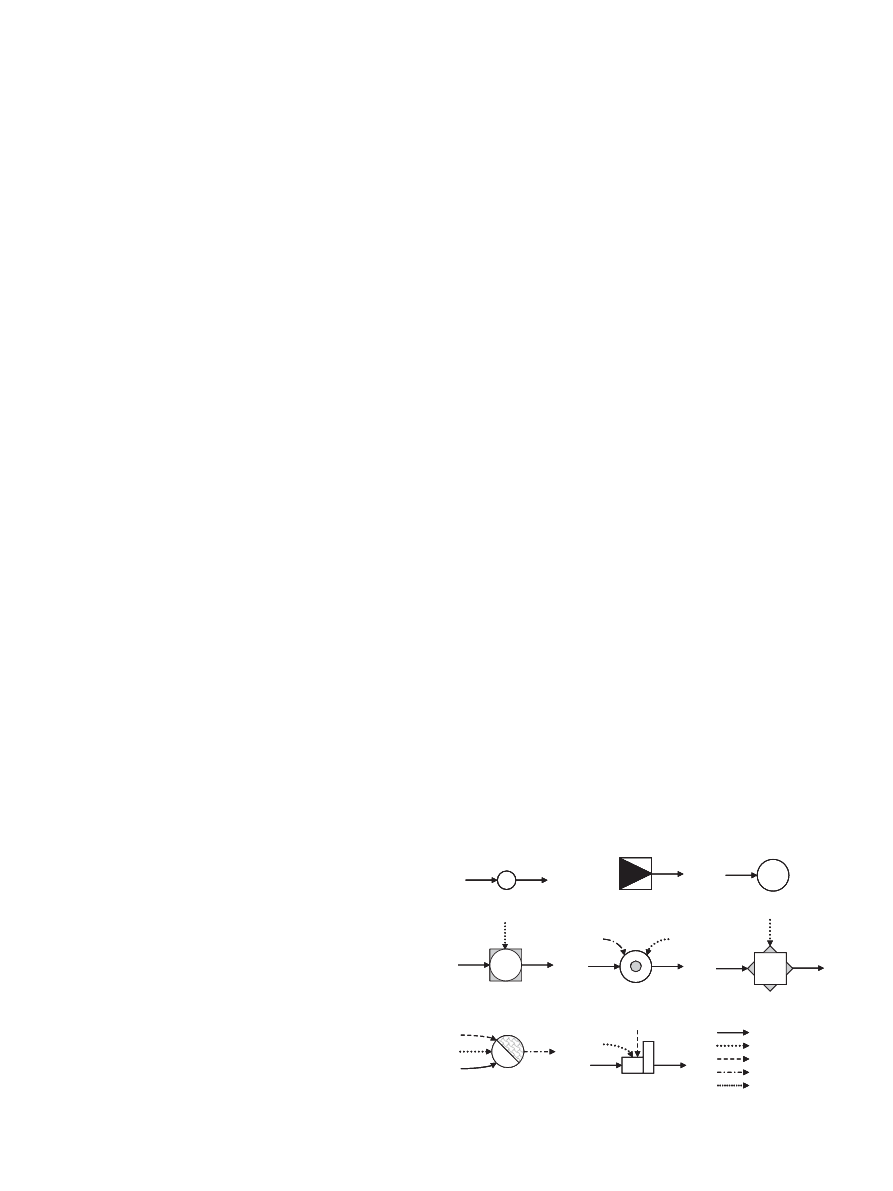
The symbolic technology models and the symbolic biomass

node are shown in

Fig. 1

. Some of the models originate from

Ref.

[18]

, but have been further developed and adjusted to the new

node structure. In the following sections, the basic structure of the
biomass module and the LP formulations for the BioNodes,
the Supply, the Dryer and the Storage model are presented in detail.
The model description is followed by a case study to illustrate the
new functionality and possible model applications.

3.1. Basic biomass module structure and biomass nodes

To be able to handle both the basic characteristics of different

kinds of biomass and the effects the variation in moisture content
might have on these properties, a set of different Products is
created. For each p ˛ Products, a reference point is speciﬁed
deﬁning the following reference parameters:

the moisture content MC

ref

the bulk density D

ref

and the heating value HV

ref

The common ﬂow variables used to model the ﬂow in the

eTransport network are (as presented in Section

): Supply_ﬂowijt,

Local_ﬂowijt, Net2net_ﬂowijt and Load_ﬂowijt. These variables only
take into account the ﬂow of energy [MW h/h] between two points
i and j in the network in different timesteps t. That is not sufﬁcient
in a biomass model, since information about the moisture content
at various steps in the chain is crucial for the optimization. For that
reason, each of the four common ﬂow variables in eTransport has
been extended with a forth index p ˛ Products to be able to repre-
sent the product properties. Thus, information about moisture
content is given and transferred between the models and the

Chipper

Biomass Node

Demand

Storage

Dryer

Supply

Combustion

Pellets Plant

Chipper

Electricity

Biomass
Fuel

Heat
Bio Oil

Fig. 1. Biomass models in eTransport – symbolic pictures.

S. van Dyken et al. / Energy 35 (2010) 1338–1350

1342

BioNodes in the network. In contrast to the common ﬂow variables,
the ﬂow between the biomass models in the network is a volume
ﬂow [m

/h] and not a ﬂow of energy. The extended ﬂow variables

are only valid in the biomass module.

Bio_supply_ﬂow

ijpt

Biomass volume ﬂow of product p from i
to j at t, where (i, j) ˛ Supply2net,
p ˛ Products and t ˛ Time_steps

Bio_local_ﬂow

ijpt

Biomass volume ﬂow of product p from i
to j at t, where (i, j) ˛ Supply2load,
p ˛ Products and t ˛ Time_steps

Bio_net2net_ﬂow

ijpt

Biomass volume ﬂow of product p from i
to j at t, where (i, j) ˛ Net2net, p ˛ Products
and t ˛ Time_steps

Bio_load_ﬂow

ijpt

Biomass volume ﬂow of product p from i to
j at t, where (i, j) ˛ Net2load, p ˛ Products
and t ˛ Time_steps

By means of the biomass node structure, the quality variable

moisture content MC

npt

is controlled in addition to the biomass

volume ﬂow. This requires the connection of each biomass model to
a biomass node. In this way, it can be accounted for that changes in
one part of the system might inﬂuence the performance of the rest
of the system. Extended passive storage keeping could for example
shorten the residence time in a dryer which in turn inﬂuences the
operating cost of the whole system.

The moisture content is modeled as a free variable which can be

restricted by different sets of parameters in the biomass nodes and
in the technology models. The biomass density and the heating
value are not separately restricted since these values are directly
linked to the moisture content assuming linear dependencies. The
biomass density in a node is linked to the moisture content by
assuming a linear dependency:

npt

¼ D

ref

1 þ MC

npt

1 þ MC

ref

; c

n˛BioNodes; p˛Products; t˛Time steps:

(1)

The density of completely dry biomass (MC

npt

¼ 0) is deﬁned

asD

zero

ref

1 þ MC

ref

; c

p˛Products:

(2)

Applying the formulation of D

zero

to Eq.

(1)

, the linear depen-

dency of biomass moisture content and density can be expressed by

npt

¼D

zero

1þMC

npt

; c

n˛BioNodes; p˛Products; t˛Timesteps:

(3)

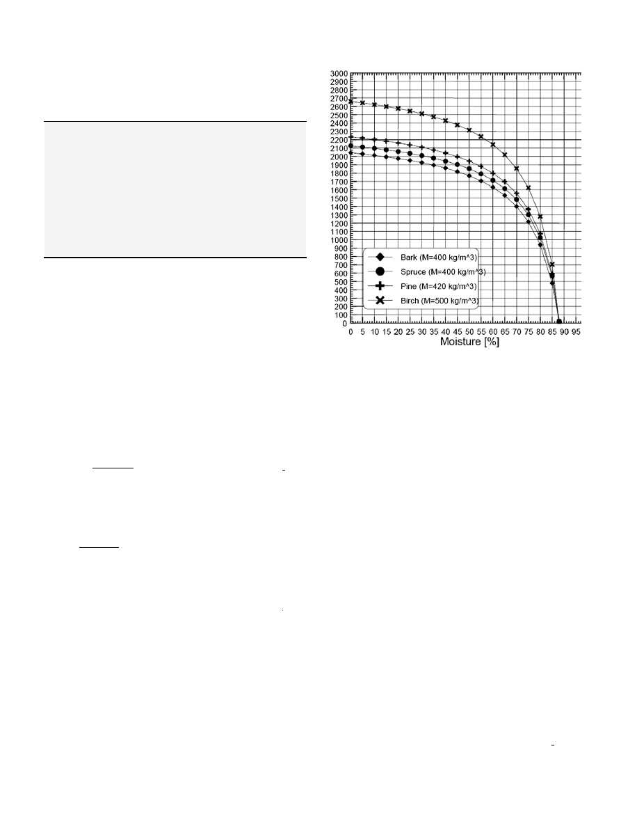
The dependency of the biomass heating value on the moisture
content is modeled by linearization of the relation shown in

Fig. 2

It is assumed that the correlation applies to all kinds of biomass.
The curve shown for spruce is taken as a reference curve. It is
divided into three linear parts using four linearization points (more
points possible for increased accuracy). The linearized curve for
spruce is scaled up and down to represent other biomass types
p ˛ Products using the corresponding reference values MC

ref

and

ref

Three different deﬁnitions are common for the heating value of

biomass:

– HHV (higher heating value) which is the gross heating value

– LHV (lower heating value) which is the net heating value. In

contrast to the HHV, the LHV does not include the heat which
originates from the water vapor formed during the combustion

– EHV (effective heating value) is the LHV subtracting the energy

of evaporating the moisture content of the biomass

The relation shown in

Fig. 2

is based on the EHV, but the

reference heating values deﬁned in the model do not necessarily
have to be the EHV. Since the dependency found based on

Fig. 2

an approximation, it is also possible to use the LHV or HHV as long
as this choice is consistent in the whole model. Furthermore, it has
to be considered that the heating values available for different
kinds of biomass often represent average values. This is caused by
the wide variation of biomass quality.

There are no operating costs associated with the biomass node

model

¼ 0:

(4)

The biomass node model does not represent a physical technology
model. It is implemented to enable the transfer of biomass property
information between the network models and to keep track of the
biomass ﬂow and the variation in moisture content. Thus, neither
the biomass volume ﬂow nor the three quality variables are modi-
ﬁed in the biomass node model. The amount of biomass that goes
into a biomass node equals the amount of biomass that leaves it. The
mass balance equation for a biomass node n ˛ BioNodes is given by

i:ði;nÞ˛Supply2net

Sup

inpt

j:ðj;nÞ˛Net2net

N2N

jnpt

l:ðn;lÞ˛Net2load

nlpt

j:ðn;jÞ˛Net2net

N2N

njpt

; c

n˛BioNodes; p˛Products; t˛Time steps:

(5)

Fig. 2. Relation between moisture content and EHV [kW h/m

S. van Dyken et al. / Energy 35 (2010) 1338–1350

1343

3.2. Supply model

The biomass supply model is a generic source that accounts for

cost and moisture content of any biomass product p. The output
volume V

bpt

BSup

cannot exceed the maximum output capacity. At the

same time, the minimum output conditions have to be kept.

Vmin

BSup
bp

BSup

bpt

Vmax

BSup
bp

;

bn˛BioSupplies; p˛Products; t˛Timesteps:

(6)

The cost of using biomass is given by

BSup

t˛Time steps

b˛BioSupplies

p˛Products

BSup

bpt

BSup

bpt

(7)

The biomass taken from a given supply point has to be fed to

a biomass node. The special properties of the biomass node system
only take effect when each model belonging to the biomass chain is
connected to a biomass node. Thus, the biomass balance for the
biomass supply point is

BSup

bpt

i:ðb;iÞ˛Supply2net

Sup

bipt

; c

b˛BioSupplies; p˛Products;

t˛Time steps:

(8)

Eq.

(8)

restricts the biomass volume ﬂow from the biomass supply

to the network. In addition, information about the moisture content
has to be transferred to the network. The moisture content in the
biomass supply is set equal to the moisture content in the biomass
node connected to the supply point. This is done applying the
general node structure and the set ‘‘Supply2net’’.

BSup

¼ if n˛BioNodes then MC

npt

else MC

BSup

;

b˛BioSupplies; ðb; nÞ˛Supply2net; p˛Products; t˛Time steps:

(9)

3.3. Dryer model

The dryer model reduces the moisture content of a biomass

product p. The heat required to run the drying process can either be
supplied by an external heat source, by direct burning of biomass or
oil, or a combination of these. The amount of biomass dried in the
model is restricted by the maximum biomass feed rate Vmax

the dryer [m

/h]. In addition, it is restricted by its rated capacity

Qmax

[MW] and the drying rate q

[kW h/kg water evaporated].

The drying rate, which is deﬁned by the user, is treated as an
average rate. It is assumed that the energy required to evaporate
the biomass moisture slightly increases when the drying is carried
out on a low moisture level. Hence, reducing the moisture content
from 60% wt to 50% wt requires less energy than reducing it from
20% wt to 10% wt. Volume losses during the drying process are
accounted for applying the volume loss coefﬁcient

(percentage

of input volume). In addition to the energy costs calculated in the
energy supply models, a speciﬁc operating cost c

per m

biomass

fed to the dryer can be speciﬁed.

The optimization of the amount of biomass fed to the dryer and

both the variable input and output moisture level leads to a non-
linear problem which has to be discretized. This is done using a set
of predeﬁned pairs of possible input and output moisture content
combinations, MCI

and MCO

. The user deﬁnes the number of

discretization points between the maximum input moisture level
MCi

and the lowest output moisture level achievable in the dryer

MCo

. The moisture pairs are generated automatically in the

model. A numerical example with the deﬁnition of MCstep

shown in

Table 1

. The optimal moisture pair is found by means of

the binary variable

dlvt

The heat required in the drying process can be obtained by

burning a fraction of the biomass. The biomass volume required to
cover the drying heat depends on the heating value of the biomass.
Again, the heating value is linked to the moisture content which is
not known before the optimization is carried out. Thus, the amount
of biomass burned for heating purposes Vb

dpt

has to be discretized,

too. This is implemented by deﬁning a certain number of dis-
cretization points Nbv

. Applying this number and the upper bound

Vbmax

, biomass volume values VB

are calculated in the model.

Due to the linear dependency of biomass density on moisture

content, the amount of water evaporated (equals the density
change) does not decrease at low moisture levels. Thus, a moisture
reduction corresponding to MCstep

always corresponds to the

same amount of water Wevap

Wevap

¼ D

zero

1 þ MCi

zero

1 þ MCi

MCstep

¼ D

zero

MCstep

; c

d˛Dryers; p˛Products:

(10)

To be able to consider a decreasing drying rate nevertheless,

a modifying factor has been implemented in the calculation of the
speciﬁc drying energy

dlp

given in Eq.

(11)

. By means of this factor,

the speciﬁc evaporation energy q

linearly increases at low drying

moisture levels.

dlp

¼ Wevap

i in Index

1 þ MCi

MCI

ði 1Þ

MCstep

; c

d˛Dryers; l˛Pairs; p˛Products:

(11)

Table 2

gives a numerical example of the modiﬁcation of q

implemented in the calculation of the speciﬁc drying energy

dlp

To maintain a linear mixed-integer problem, both the input and

output moisture content has to be further restricted. This is done by
applying the predeﬁned discretization moisture pairs. The binary
variable

dlvt

is implemented to select the most suitable moisture

pair. The values of

dlvt

are set by the solver. The constraint given by

l˛Pairs;v˛Burn

Dr
dlvt

¼ 1; cd˛Dryers; t˛Time steps

(12)

Table 1
Example: generation of moisture pairs for discretization in dryer model.

Parameter data

MCi

¼ 0:6

MCo

¼ 0:4

Nli

¼ 3

Nsteps

¼ 4

Npairs

¼ 15

MCstep

¼ ðMCi

MCo

Þ=Nsteps

¼ 0:05

40 %

60 %

point

step

Dr
d

MCi

Dr
d

MCo

40 %

60 %

point

step

Dr
d

MCi

Dr
d

MCi

Dr
d

MCo

Dr
d

MCo

Generated moisture pairs

(0.60/0.60)

(0.60/0.55)

(0.60/0.50)

(0.60/0.45)

(0.60/0.40)

(0.55/0.5)

(0.55/0.50)

(0.55/0.45)

(0.55/0.40)

(0.50/0.50)

(0.50/0.45)

(0.50/0.40)

(0.45/0.45)

(0.45/0.40)
(0.40/0.40)

S. van Dyken et al. / Energy 35 (2010) 1338–1350

1344

assures that only one

dlvt

is set to equal one. Thus, only one

moisture pair (the most appropriate one) is chosen. This choice is
taken by the solver considering the other constraints and the cost
functions.

Eqs.

(13) and (14)

restrict the difference between input and

output moisture (the level of moisture reduction in the dryer),
applying the combinations given by the moisture discretization
pairs.

MCin

dpt

l˛Pairs;v˛Burn

MCI

Dr
dlvt

;

(13)

MCout

dpt

l˛Pairs;v˛Burn

MCO

Dr
dlvt

; c

d˛Dryers; l˛Pairs;

p˛Products; t˛Time steps:

(14)

In the same way as the moisture level, the amount of biomass

burned has to be restricted by applying the discretized values VB

and the binary variable

dlvt

dpt

l˛Pairs;v˛Burn

Dr
dlvt

; c

d˛Dryers; p˛Products;

t˛Time steps:

(15)

The energy required to reduce the biomass moisture in the dryer

is calculated by means of the speciﬁc drying energy

dlp

and given

dpt

dlp

Vin

dpt

v˛Burn

Dr
dlvt

dlp

Vmax

;

d˛Dryers; l˛Pairs; p˛Products; t˛Time steps:

(16)

The heat required to dry the biomass volume can either be supplied
by an external heat source or by burning biomass or oil. The heating
value HVin

dlp

of the biomass input volume is calculated applying

the dependency described in Section

3.2

, subject to the moisture

pairs given for discretization. The amount of drying heat cannot
exceed the drying heat capacity of the dryer:

dpt

Qex

þ F

dpt

HVoil þ

l˛Pairs;v˛Burn

HVin

dlp

dlvt

;

(17)

where

dpt

Q max

; c

d˛Dryers; p˛Products; t˛Time steps:

(18)

It is assumed that some of the biomass gets lost or becomes

unusable during the drying process. This is modeled by deﬁning
a certain percentage of the input volume as loss volume (Eq. (

)).

Furthermore, the input volume cannot exceed the maximum input
capacity (Eq. (

)):

Vin

dpt

¼ Vout

dpt

1 þ

;

(19)

where

Vin

dpt

Vmax

; c

d˛Dryers; p˛Products; t˛Time steps:

(20)

The operating costs of the dryer model are energy costs which

are calculated in the supply models. Fuel costs due to oil use F

dpt

external heat use Qex

or the cost for the biomass burned in the

dryer are accounted for in the oil supply, the external heat supply
and the biomass supply model object function, respectively. An oil-
ﬁred dryer causes emission, and the emission costs are calculated
as given in Eq.

(21)

, provided that an emission penalty Pen

deﬁned.

e˛Emissions

t˛Time steps

d˛Dryers

Pen

Emit

edt

;

(21)

where

Emit

edt

¼ em

dpt

HVoil; cp˛Products; d˛Dryers;

t˛Time steps; e˛Emissions:

(22)

The amount of biomass ﬂowing to the dryer is the sum of the

biomass volume dried and the (optional) biomass volume burned
to supply drying heat. The biomass is fed to the dryer from the
biomass node n connected to the dryer input point i. The input and
output volume is linked by Eq.

(19)

. The dried biomass is sent to the

biomass node n connected to the dryer output point j:

Vin

dpt

þ Vb

dpt

i:ðn;iÞ˛Net2net

N2N

nipt

;

(23)

Vout

dpt

j:ðj;nÞ˛Net2net

N2N

jnpt

; c

d˛Dryers; n˛BioNodes;

p˛Products; t˛Time steps:

(24)

The biomass moisture content at the dryer inlet (outlet) is set

equal to the moisture content in the biomass node connected to the
dryer inlet (outlet). This is done applying the general node structure
and the set ‘‘Net2net’’.

MCin

dpt

¼ if n˛BioNodes then MC

npt

; c

d˛Dryers;

ðn; dÞ˛Net2net; p˛Products; t˛Time steps;

(25)

MCout

dpt

¼ if n˛BioNodes then MC

npt

; c

d˛Dryers;

ðd; nÞ˛Net2net; p˛Products; t˛Time steps:

(26)

In addition to the heat obtained by burning biomass in the dryer,

it is possible to reuse external waste heat or to produce drying heat
from burning oil. The energy balance for the dryer heat input point
h and the dryer fuel input point f is

Qex

h:ði;hÞ˛Net2net

N2N

iht

h:ðs;hÞ˛Supply2net

Sup

sht

;

(27)

dpt

HVoil ¼

f :ði;f Þ˛Net2net

N2N

ift

f :ðs;f Þ˛Supply2net

Sup

sft

;

d˛Dryers; t˛Time steps:

(28)

Table 2
Example: calculation of speciﬁc drying energy in dryer model.

MCi

MCo

, const

0.6

0.2

2.0

MCI

MCO

, mod

0.6

0.5

2.0

0.6

0.4

2.1

0.6

0.3

2.2

0.6

0.2

2.3

0.5

0.4

2.2

0.5

0.3

2.3

0.5

0.2

2.4

0.4

0.3

2.4

0.4

0.2

2.5

0.3

0.2

2.6

S. van Dyken et al. / Energy 35 (2010) 1338–1350

1345

Here, the common energy ﬂow variables are used, since no

information on biomass quality is required. The biomass chain thus
interacts directly with the other energy carriers in the system.

3.4. Storage model

Any biomass product can be sent to the storage model. In

addition to the energy storage function, the model provides the
opportunity to indicate passive drying effects as a function of the
storage time. The passive drying function is not appropriate for an
hourly time resolution, but it becomes applicable when the analysis
is carried out on a weekly basis as described in Section

. However,

the passive drying functionality is deﬁned per timestep and is not
limited to a certain time resolution. To indicate internal fuel use due
to biomass handling in the storage, a fuel input point is also deﬁned.

The drying rate

is user-deﬁned and describes the reduction of

biomass moisture (percentage) which can be achieved per time-
step. In addition to the moisture reduction coefﬁcient, the volume
loss coefﬁcient

and the storage cost coefﬁcient c

are also

deﬁned per timestep.

Similarly to the drying model, the moisture reduction coefﬁcient

is treated as an average input value. However, in contrast to the
dryer model, the decreasing drying rate at lower moisture levels is
not implemented. It is assumed that the moisture reduction rate
decreases with increasing storage time Tout

Tin

, expressed in

parameter

spab

. The volume loss coefﬁcient is dealt with in the

same way: The volume losses are increasing with increasing
storage time, expressed in the calculated parameter E

spab

. In this

way, volume and quality losses due to long-term storage can be
indicated. The storage cost is deﬁned per timestep, too, but the cost
is assumed as constant and summed up over the total storage time
in the parameter C

sab

. That means that no cost increase due to

increasing storage time is implemented.

The binary variable

spab

keeps track of how long (how many

timesteps) the biomass at least has to be stored to reach the
moisture level required at the storage output. It is not possible to
take out biomass with a moisture level higher than that one
required at the storage output point.

It is assumed that increasing storage time has an impact on both

the moisture reduction coefﬁcient

and the volume loss coefﬁ-

cient

. The storage costs are assumed to be stable, thus they do

not change with increasing storage time and are constant in each
timestep. The total storage costs are calculated by multiplying the
cost coefﬁcient by the number of timesteps spent between input
and output of biomass to/from storage (Tout

Tin

) given by

sab

¼ if Tin

¼ Tout

then 0 else c

Tout

Tin

;

s˛Storages; ab˛Time steps:

(29)

Another assumption is that the longer the biomass is stored, the

more volume gets lost (due to biomass handling). In addition to
handling losses, other negative effects may appear (quality loss due
to e.g. fungal decay). These effects are modeled by deﬁning
a volume loss parameter dependent on storage time:

spab

¼ if Tin

¼ Tout

then 1 else

Tout

Tin

St
sb

;

s˛Storages; p˛Products; ab˛Time steps:

(30)

An increasing time difference between biomass input and

output of the same volume leads to growing volume losses. The
equation implemented to express a decreasing drying rate is
comparable to the volume loss calculation in Eq.

(30)

. The mode of

calculation of both factors is based on assumptions. It is assumed
that less moisture is evaporated when the biomass already has

been stored for a long time. This offers the possibility to display the
decelerated drying effect at lower moisture levels in the model.
Contrary to the volume loss calculation, the decreasing drying rate
is still deﬁned per timestep, given by

St
spab

¼ if Tin

¼ Tout

then

St
sp

else

St
sp

Tout

Tin

Tout

Tin

;

s˛Storages; p˛Products; ab˛Time steps:

(31)

Table 3

gives a numerical example of the calculation of both the

time-dependent parameters

spab

and E

spab

and the constant cost

parameter C

sab

in the storage model.

The user deﬁnes whether passive drying effects occur during

storage or not. This is done by implementing the binary parameter

. If

is set to zero (no passive drying in storage), the storage time

is not restricted. That means that the optimization algorithm
chooses freely (only restricted by the storage cost in the objective
function) for how many timesteps the biomass is stored and when it
is sent to the next biomass model in the supply chain. However, if

is set to one (passive drying effects in storage), time-dependent
restrictions have to be met. In this case, the storage time is restricted
applying the binary variable

spab

. Considering the maximum and

minimum values of moisture content given in the biomass node at
the storage output or the demand moisture level in the end of the
supply chain, a certain moisture range for the storage output
moisture level is deﬁned. Applying the binary variable

spab

and the

drying rate

spab

, it is calculated how many timesteps the biomass

has to be stored to reach the output moisture level required:

St
spab

Tout

Tin

MCin

spt

MCout

spt

St
spab

;

(32)

St
spab

Tout

Tin

MCin

spt

MCout

spt

St
spab

;

s˛Storages; p˛Products; ab˛Time steps:

(33)

spab

is set to one if the output moisture level can be reached

during the time period Tin

Tout

, otherwise it is set to zero. It is

assumed that some of the biomass gets lost or becomes unusable
during the storage process. This is modeled by deﬁning a certain
percentage of the input volume as loss volume. The biomass
volume ﬂow to and from storage is restricted by

Vin

spt

b˛Time steps

Vtrans

spab

;

(34)

Vout

spt

a˛Time steps

Vtrans

spab

;

(35)

Table 3
Example: calculation of constants in storage model.

0.05

0.01

200

Tout

Tin

spab

sab

0.0500

0.9900

200

0.0488

0.9801

400

0.0475

0.9703

600

0.0464

0.9606

800

0.0452

0.9510

1000

S. van Dyken et al. / Energy 35 (2010) 1338–1350

1346

where

Vtrans

spab

St
spab

Vmax

s˛Storages; p˛Products;ab˛Timesteps:

(36)

where the volume loss factor E

spab

is deﬁned in Eq.

(30)

The user-deﬁned cost factor is multiplied by the biomass

volume Vtrans

spab

handled in storage to determine the storage cost:

a;b˛Time steps

s˛Storages

p˛Products

sab

Vtrans

spab

e˛Emissions

Pen

Emit

est

(37)

where

Emit

est

¼ em

HVoil$Vin

spt

; c

p˛Products; s˛Storages;

a; b˛Time steps; e˛Emissions:

(38)

Storage keeping causes emissions only when an external fuel
demand is deﬁned, applying the parameter F

. In this case, the

emission costs are added to the operating costs, provided that an
emission penalty Pen

is deﬁned. Fuel costs are accounted for in

the oil supply model objective.

The biomass is fed to the storage from the biomass node n

connected to the storage input point i and sent from the storage to
the biomass node n connected to the storage output point j

Vin

spt

i:ðn;iÞ˛Net2net

N2N

nipt

;

(39)

Vout

spt

j:ðj;nÞ˛Net2net

N2N

jnpt

; c

s˛Storages; n˛BioNodes;

p˛Products; t˛Time steps;

(40)

applying the biomass ﬂow variable V

jnpt

(Bio_net2net_ﬂowijpt).

The input and output volume is linked by Eq.

(34) and (35)

. Simi-

larly to the dryer model with Eq.

(25) and (26)

, the biomass

moisture content at the storage inlet (outlet) is set equal to the
moisture content in the biomass node connected to the storage
inlet (outlet):

MCin

spt

¼ if n˛BioNodes then MC

npt

; c

s˛Storages;

ðn; sÞ˛Net2net; p˛Products; t˛Time steps;

(41)

MCout

spt

¼ if n˛BioNodes then MC

npt

; c

s˛Storages;

ðs; nÞ˛Net2net; p˛Products; t˛Time steps:

(42)

The fuel needed by the storage to handle the biomass is fed from

the network to the storage fuel input point f.

HVoil$Vin

spt

f :ði;f Þ˛Net2net

N2N

ift

f :ðs;f Þ˛Supply2net

Sup

sft

;

d˛Storages; t˛Time steps:

(43)

According to Eq.

(28)

in the dryer model, the common energy

ﬂow variables are used, since no information on biomass quality
parameters is required.

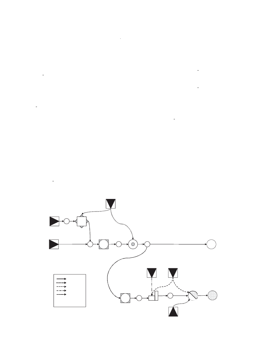
4. Case study

To demonstrate the use of the new biomass models, especially

the functionality of the active and passive drying processes in the
Dryer and Storage model, a simple case study is carried out. The
main intention is to point out the properties and functionality of
the new models rather than to represent a detailed analysis of a real
biomass supply chain with several alternatives. Therefore, no
investment analysis is carried out and the emissions caused by the

BIO_SUP_S

CHIP

STOR_I

DRY

STOR_II

HEAT LOAD

BIO_LOAD_C

BIO_SUP_C

FUEL_SUP_I

EL_SUP

FUEL_SUP_II

HEAT_SUP

0.5

0.1

0.11

0.5

Electricity

Biomass
Fuel

Heat
Bio Oil

0.5

Moisture

content

Fig. 3. Biomass case in eTransport.

S. van Dyken et al. / Energy 35 (2010) 1338–1350

1347

different processes applied in the case are not investigated. Only
limited focus has been given to obtain realistic input data.

4.1. Case overview

The analysis is run over a time period of twelve weeks (twelve

timesteps t). This period is appropriate to describe the active drying
processes in the dryer and to allow for moisture decrease from one
week to another in the storage model.

It is assumed that the amount of biomass products available

within a time period of twelve weeks varies. Thus, the biomass
supply proﬁle is not constant, but the biomass demand proﬁle is
assumed to be constant. Hence, storage keeping is required to be
able to cover the demand in all weeks. The combination of moisture
content demanded at different points in the case is set in such
a way that both passive and active drying processes are possible.

The case setup is shown in

Fig. 3

. Three different biomass

products are handled in the case: spruce, chips and pellets with the
reference values given in

Table 4

. On the demand site, there is

a biomass load point demanding chips at a constant level of
100 m

/week (average 0.6 m

/h) and a heat load point with

a demand of 20 MW h/week (average 119 kW h/h). To cover the
demand, two different biomass supplies with restricted capacities
are available: a chip supply (45 USD/m

) and a spruce supply

(35 USD/m

). As can be seen from

Fig. 4

, the chip supply volume is

not sufﬁcient to cover the chip demand. Thus, chips have to be
processed from spruce in the chipper before they are sent to
storage. This increases the price (spruce) due to the additional
energy costs generated in the chipper.

The moisture content required in the different supply, conver-

sion and load points is indicated in the case setup in

Fig. 3

. Both the

chips and the spruce are supplied with a moisture content of 50%
wt. The moisture content demanded by the biomass load (chips) is
11% wt while the moisture content of the biomass burned in the
boiler cannot exceed 10% wt. Thus, drying is required. This can be
carried out either active in the dryer or passive in the storages. In
both storage models, the drying option is enabled and it is assumed
that the moisture content of the biomass stored is reduced with 1%

wt during one week. The speciﬁc energy required in the dryer to
evaporate one kg of water from biomass is set to 2 kW h/kg
(average heat requirement for dryers

[19]

After having passed the dryer, the main fraction of chips is sent

to the biomass demand point. The remaining chips are sent to
a second storage which is followed by a combination of a pellets
production plant and a boiler to cover the heat demand. The drying
heat required in the dryer is supplied both by an external heat
source (restricted capacity) and by burning fuel. The option of
burning biomass is not used. The heat required in the pellet
production plant is covered by an external heat source, too. Both
the pellet plant and the boiler demand electricity to run internal
control systems and other supplementary devices. The amount of
energy required to handle the biomass inside storage is neglected.
Similarly, no additional operating costs are deﬁned.

Apart from the combustion model, the maximum capacity

(volume and heat) in the conversion models is not restricted. In the
combustion model, the maximum volume capacity is limited so
that the integrated additional oil ﬁring option has to be applied. The
volume losses are set to 1% of the input volume in the storage and
the dryer model, while losses of 5% are assumed in the chipper and
the pellet plant. There is no cost associated with the use of external
heat. The fuel cost is set to 0.65 USD/liter, the electricity cost to
84 USD/MW h.

4.2. System operation and results

The model chooses from the two supply sources available as

shown in

Fig. 5

. The volume capacity of the spruce supply is utilized

fully while the chips supply only is used to cover lacking chips
production. With the cost combination deﬁned in the model, it is
more proﬁtable to process chips from spruce and to pay for the fuel
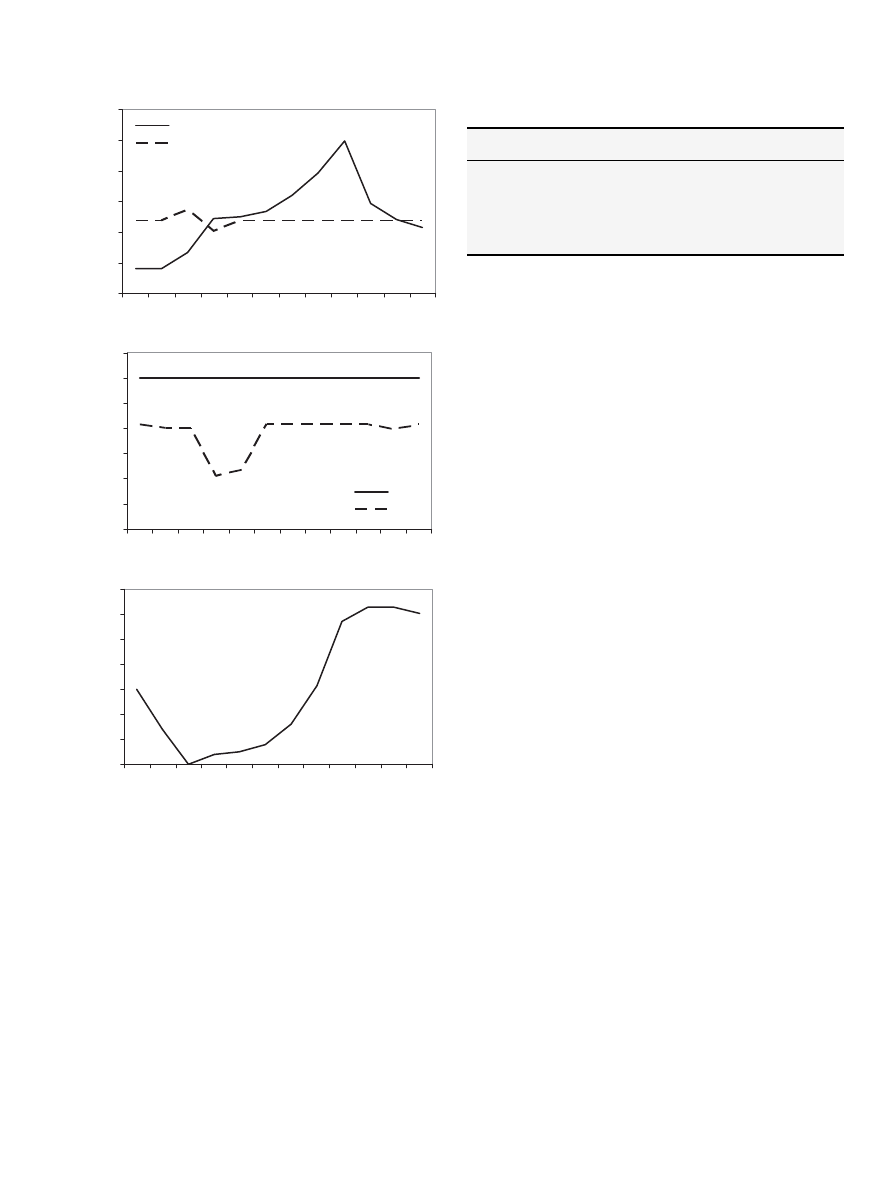
required in the process than to purchase chips directly from supply.

Fig. 6

illustrates both the drying effect and the storage keeping

in storage I. The moisture content is reduced from 50% wt at the
storage input to values in the range between 46.4% wt and 42.3% wt.
The lowest output moisture content is reached in week four. One
has to keep in mind that the set Time_steps is deﬁned as circular.
Thus, week twelve is followed by week one in the model. A certain
amount of biomass sent to storage in week seven for instance might
be sent out in week four. This leads to a storage time of nine weeks
associated with a fairly high moisture reduction. As can be seen
from

Fig. 6

(a) and (c) the storage is ﬁlled to a high level to take

advantage of the increasing moisture reduction with longer storage
time.

In storage II, the moisture content of the chips is reduced from

11% wt (dryer output) to 10% wt (boiler input required). With the

Table 4
Reference values of case products.

Parameter

Unit

Spruce

Chips

Pellets

ref

%wt

ref

kg/m

405

340

700

ref

kW h/m

2155

1000

3200

100

120

140

160

180

weeks

Volume [m

]

Spruce
Chips

Fig. 4. Maximum volume capacity spruce and chips supply.

100

150

200

250

weeks

]

Chips
Spruce

Fig. 5. Total output volume spruce and chips supply.

S. van Dyken et al. / Energy 35 (2010) 1338–1350

1348

moisture reduction factor of 1% wt assumed in storage II, the
requested moisture level can be reached during one week. Thus,
chips sent to storage in one week are sent out with a moisture level
of 10% wt in the following week. Therefore, in contrast to storage I,
no remarkable storage effects are to be observed in storage II.

The objective value represents the operating cost for the whole

system. Over a time horizon of twelve weeks the operating cost
adds up to 68,733.51 USD. This value represents the fuel cost, the
biomass cost and the electricity cost.

5. Discussion

The objective of the present work is to develop a linear

modeling framework as a part of the eTransport optimization tool
that can be applied to most relevant components in a biomass
supply chain, including sources, handling/processing, storage and

end use. The moisture content has large inﬂuence on the efﬁciency
of various biomass conversion processes like combustion and
pyrolysis

[20]

. Thus, the main focus of this work has been to

represent the relationship between moisture and energy content of
different kinds of biomass and to handle long-term processes in the
optimization like passive drying effects.

With the modeling approach presented in this paper, a solid basis

for the linear modeling of general biomass supply chains has been
developed. Due to assumptions and simpliﬁcations made in the models
as well as the fact that the biomass module is embedded in the already
existing eTransport framework, there are some model limitations.

The modeling of long-term effects in the biomass module is

a new approach which is partly limited by the time structure in
eTransport. Long-term effects in the biomass models can be
a challenge when combined with shorter time resolution e.g. in
heat and electricity loads. In the case study presented this has been
solved by using weekly average values.

Another time aspect in the model is the solving time. It varies

with the complexity of the problem depending on system size, the
range of products to be handled and the number of timesteps
chosen. One possibility to avoid prohibitive solving times is to
lower the precision of the solver. This can be justiﬁed by the fact
that uncertainty in the input dataset contributes signiﬁcantly more
to the total uncertainty of the objective value than the gap between
the best feasible solution and its lower bound. To illustrate this, the
case presented has been solved with a range of allowed gaps in the
CPLEX branch and bound algorithm. The resulting solving time and
objective values are given in

Table 5

. As seen from the table the

solution time is reduced by a factor of 100 by increasing the allowed
gap from 5% to 10% of lower bound on the objective value.

The economic part of the biomass model application and the

emission handling are not discussed in detail since the calculation
follows the main eTransport algorithms documented in

[14]

. Emis-

sions can be accounted for both in biomass sources (due to harvesting,
handling, etc.), energy use in biomass processing models and from
combustion. These emissions are then considered by the investment
algorithm in the same way as for other combustion models.

In the case study, only limited focus has been given to obtain

realistic input data. The main objective with the case study is to
demonstrate the functionality of the new methodology presented.
The assembly of models shown in the case study represents one
possibility out of an unlimited number of combinations. With the
data chosen, the functionality available in the biomass models is
demonstrated. A next step in the model development and
improvement would be to validate the results with working
conditions of a real system.

6. Summary

Both the eTransport model and the biomass module discussed

in this paper are still under development. The biomass models are
partly an expansion of models from a master thesis

[18]

. The work

100

150

200

250

300

10 11 12

weeks

volume [m

]

input
output

0,38

0,40

0,42

0,44

0,46

0,48

0,50

0,52

10 11 12

weeks

moisture content

input
output

100

150

200

250

300

350

10 11 12

weeks

volume [m

]

Fig. 6. Storage I, (a) input and output volume, (b) moisture content, (c) volume stored.

Table 5
Solving time and objective value for a range of gap tolerances in the solver.

MIPGAP [% of lower bound
on objective value]

Solving
time [s]

Objective
value [USD]

7.07

69,123.7003

7.83

69,123.7003

14.12

69,028.6076

37.86

68,910.7083

159.06

68,733.5117

747.70

68,733.5117

1 h

S. van Dyken et al. / Energy 35 (2010) 1338–1350

1349

presented in this paper has been carried out with ﬁnancial support
from the Research Council of Norway and StatoilHydro. Require-
ments from StatoilHydro have inﬂuenced the technologies to be
modeled. In addition to the seven biomass models presented in
Section

, two more models have been developed:

Transport: Truck transport. Discrete model, emissions due to fuel
use.
Pyrolysis: Bio oil production in a fast pyrolysis process. Link to
bio fuel applications.

These two models are not discussed in detail, but they illustrate

the many possibilities for further development of the biomass
module. The transport model is a discrete model. The pyrolysis
model can be seen as a link to bio fuel applications. This link shows
the wide variety of biomass utilization. Other processing technol-
ogies as for instance bundling and grinding could be implemented
in future. Moisture dependent efﬁciency of biomass combustion
models can also be implemented within the new framework. The
whole biomass sector itself is under development and new and
more improved technologies frequently appear. With its ﬂexible
structure, the biomass module presented here is a solid basis for
further development and improvement.

Acknowledgements

The authors gratefully acknowledge the support from the

Research Council of Norway and from StatoilHydro as a sponsor of
the project.

References

[1] International Energy Agency. IEA bioenergy – an international collaboration in

bioenergy. See also,

http://www.ieabioenergy.com

[accessed 1.02.09].

[2] European Union Energy Research – Biomass. See also,

http://ec.europa.eu/

research/energy/nn/nn_rt/nn_rt_bm/article_1110_en.htm

[accessed 1.02.09].

[3] Sokhansanj S, Kumar A, Turhollow AF. Development and implementation of

integrated biomass supply analysis and logistics model (IBSAL). Biomass and
Bioenergy 2006;30:838–47.

[4] Freppaz D, Minciardi R, Robba M, Rovatti M, Sacile R, Taramasso A. Optimizing

forest biomass exploitation for energy supply on a regional level. Biomass and
Bioenergy 2004;26:15–25.

[5] Gigler JK, Hendrix EMT, Heesen RA, van den Hazelkamp VGW, Meerdink G. On

optimization of agri chains by dynamic programming. European Journal of
Operational Research 2002;139:613–25.

[6] Frombo F, Minciardi R, Robba M, Sacile R. A decision support system for

planning biomass-based energy production. Energy 2009;34:362–9.

[7] Kumar A, Sokhansanj S, Flynn PC. Development of a multicriteria assessment

model for ranking biomass feedstock collection and transportation systems.
Applied Biochemistry and Biotechnology 2006;123:71–87.

[8] Nagel J. Determination of an economic energy supply structure based on

biomass using a mixed-integer linear optimization model. Ecological Engi-
neering 2000;16:91–102.

[9] Rentizelas AA, Tolis AJ, Tatsiopoulos IP. Logistics issues of biomass: the storage

problem and the multi-biomass supply chain. Renewable and Sustainable
Energy Reviews 2009;13:887–94.

[10] Mahmoudi M, Sowlati T, Sokhansanj S. Logistics of supplying biomass from

a mountain pine beetle-infested forest to a power plant in British Columbia.
Scandinavian Journal of Forest Research 2009;24:76–86.

[11] Bakken BH, Wolfgang O, Roynstrand J, Frydenlund F, Skjelbred HI. eTransport:

a novel tool for energy system planning. Report A6255. Trondheim, Norway:
SINTEF Energy Research, ISBN 82-594-2966-7; 2006.

[12] Bakken BH, Holen AT. Energy service systems: integrated planning case

studies. In: Proceedings of the IEEE Power Engineering Society 2004 general
meeting, Denver, CO, USA, 2004. IEEE; 2004.

[13] Bakken BH, Velken I. Linear models for optimization of infrastructure for CO

capture and storage. IEEE Transactions on Energy Conversion 2008;23:
824–33.

[14] Bakken BH, Wolfgang O, Skjelbred HI. eTransport: investment planning in

energy supply systems with multiple energy carriers. Energy 2007;32:
1676–89.

[15] Fourer R, Gay DA, Kerninghan BW. AMPL: a modeling language for mathe-

matical programming. Toronto: Thomson; 2003.

[16] Tomasgard A, Bjørndal M, Midthun K. Modeling optimal economic dispatch

and ﬂow externalities in natural gas networks. In: Proceedings of the Trans-
Atlantic Infraday, conference on applied infrastructure modeling and policy
analysis, Maryland, USA; 2007.

[17] Midthun K. Optimization models for liberalized natural gas markets. Doctoral

thesis, Norwegian University of Science and Technology, Trondheim, Norway;
2007. ISBN 978-82-471-4526-5.

[18] Li Y. Modelling of infrastructure for biomass collection. Master thesis,

Norwegian University of Science and Technology, Trondheim, Norway; 2006.

[19] Amos WA. Report on biomass drying technology. Report NREL/TP-570-

25885. 1617 Cole Boulevard, Golden, CO, USA: National Renewable Energy
Laboratory; 1998.

[20] Yoshida Y, Dowaki K, Matsumura Y, Matsuhashi R, Li D, Ishitani H, et al.

Comprehensive comparison of efﬁciency and CO

emissions between biomass

energy conversion technologies – position of supercritical water gasiﬁcation
in biomass technologies. Biomass and Bioenergy 2003;25:257–72.

S. van Dyken et al. / Energy 35 (2010) 1338–1350

1350

Document Outline

Linear mixed-integer models for biomass supply chains with transport, storage and processing

Wyszukiwarka

Podobne podstrony:
36 495 507 Unit Cell Models for Thermomechanical Behaviour of Tool Steels
key pro m8 supported models for vw
Advanced Methods for Development of Wind turbine models for control designe
ANIMAL MODELS FOR IMPLANT BIOMA Nieznany (2)
Time Series Models For Reliability Evaluation Of Power Systems Including Wind Energy
Energy and CO2 analysis of poplar and maize crops for biomass production in Italy Włochy 2016
Queuing theory based models for studying intrusion evolution and elimination in computer networks
RFID Security Issues in Military Supply Chains
One hit models for virus inactivation studies
Cost Models for Future Software Life Cycle Processes; COCOMO 2 0 Barry Boehm et al
Barret et al Templates For The Solution Of Linear Systems Building Blocks For Iterative Methods [s
Models for drying kinetics based on drying curves of slabs
(paper)Learning Graphical Models for Stationary Time Series Bach and Jordan
choi t m chiu c h risk analysis in stochastic supply chains

więcej podobnych podstron

Linear mixed integer models for biomass supply chains with transport, storage

Document Outline