
Ecient Collision Detection for
Animation and Robotics
Ming C. Lin
Department of Electrical Engineering
and Computer Science
University of California, Berkeley
Berkeley, CA,

Ecient Collision Detection for Animation and Robotics
by
Ming Chieh Lin
B.S. (University of California at Berkeley) 1988
M.S. (University of California at Berkeley) 1991
A dissertation submitted in partial satisfaction of the
requirements for the degree of
Doctor of Philosophy
in
Engineering - Electrical Engineering
and Computer Sciences
in the
GRADUATE DIVISION
of the
UNIVERSITY of CALIFORNIA at BERKELEY
Committee in charge:
Professor John F. Canny, Chair
Professor Ronald Fearing
Professor Andrew Packard
1993

Ecient Collision Detection for Animation and Robotics
Copyright
c
1993
by
Ming Chieh Lin

i
Abstract
Ecient Collision Detection for Animation and Robotics
by
Ming Chieh Lin
Doctor of Philosophy in Electrical Engineering
and Computer Science
University of California at Berkeley
Professor John F. Canny, Chair
We present ecientalgorithms for collision detection and contact determina-
tion between geometric models, described by linear or curved boundaries, undergoing
rigid motion. The heart of our collision detection algorithm is a simple and fast
incremental method to compute the distance between two convex polyhedra. It uti-
lizes convexity to establish some local applicability criteria for verifying the closest
features. A preprocessing procedure is used to subdivide each feature's neighboring
features to a constant size and thus guarantee expected constant running time for
each test.
The expected constant time performance is an attribute from exploiting the
geometric coherence and locality. Let
n be the total number of features, the expected
run time is between
O(
p
n) and O(n) depending on the shape, if no special initial-
ization is done. This technique can be used for dynamic collision detection, planning
in three-dimensional space, physical simulation, and other robotics problems.
The set of models we consider includes polyhedra and objects with surfaces
described by rational spline patches or piecewise algebraic functions. We use the
expected constant time distance computation algorithm for collision detection be-

ii
tween convex polyhedral objects and extend it using a hierarchical representation to
distance measurement between non-convex polytopes. Next, we use global algebraic
methods for solving polynomial equations and the hierarchical description to devise
ecient algorithms for arbitrary curved objects.
We also describe two dierent approaches to reduce the frequency of colli-
sion detection from
0
@
N
2
1
A
pairwise comparisons in an environment with
n moving
objects. One of them is to use a priority queue sorted by a lower bound on time to
collision; the other uses an overlap test on bounding boxes.
Finally, we present an opportunistic global path planner algorithm which
uses the incremental distance computation algorithm to trace out a one-dimensional
skeleton for the purpose of robot motion planning.
The performance of the distance computation and collision detection algo-
rithms attests their promise for real-time dynamic simulations as well as applications
in a computer generated virtual environment.
Approved: John F. Canny

iii
Acknowledgements
The successful completion of this thesis is the result of the help, coop-
eration, faith and support of many people.
First of all, I would like to thank Professor John Canny for the in-
sightful discussions we had, his guidance during my graduate studies at
Berkeley, his patience and support through some of the worst times in
my life. Some of the results in this thesis would not have been possible
without his suggestions and feedbacks.
I am also grateful to all my committee members (Professor R. Fear-
ing, A. Packard, and J. Malik), especailly Professor Ronald Fearing and
Andrew Packard for carefully proofreading my thesis and providing con-
structive criticism.
I would like to extend my sincere appreciation to Professor Dinesh
Manocha for his cheerful support and collaboration, and for sharing his
invaluable experience in \job hunting". Parts of Chapter 4 and a section
of Chapter 5 in this thesis are the result of our joint work.
Special thanks are due to Brian Mirtich for his help in re-implementing
the distance algorithm (described in Chapter 3) in ANSI C, thorough
testing, bug reporting, and his input to the robustness of the distance
computation for convex polyhedra.
I wish to acknowledge Professor David Bara at Carnegie Mellon Uni-
versity for the discussion we had on one-dimensional sweeping method. I
would also like to thank Professor Raimond Seidel and Professor Herbert
Edelsbrunner for comments on rectangle intersection and convex decom-
position algorithms; and to Professor George Vanecek of Purdue Univer-
sity and Professor James Cremer for discussions on contact analysis and
dynamics.
I also appreciate the chance to converse about our work through elec-
tronic mail correspondence, telephone conversation, and in-person inter-
action with Dr. David Stripe in Sandia National Lab, Richard Mastro and
Karel Zikan in Boeing. These discussions helped me discover some of the
possible research problems I need to address as well as future application
areas for our collision detection algorithms.

iv
I would also like to thank all my long time college pals: Yvonne and
Robert Hou, Caroline and Gani Jusuf, Alfred Yeung, Leslie Field, Dev
Chen and Gautam Doshi. Thank you all for the last six, seven years of
friendship and support, especially when I was at Denver. Berkeley can
never be the same wthout you!!!
And, I am not forgetting you all: Isabell Mazon, the \Canny Gang",
and all my (30+) ocemates and labmates for all the intellectual conver-
sations and casual chatting. Thanks for the #333 Cory Hall and Robotics
Lab memories, as well as the many fun hours we shared together.
I also wish to express my gratitude to Dr. Colbert for her genuine care,
100% attentiveness, and buoyant spirit. Her vivacity was contagious. I
could not have made it without her!
Last but not least, I would like to thank my family, who are always
supportive, caring, and mainly responsible for my enormous amount of
huge phone bills. I have gone through some traumatic experiences during
my years at CAL, but they have been there to catch me when I fell, to
stand by my side when I was down, and were
ALWAYS
there for me no
matter what happened. I would like to acknowledge them for being my
\moral backbone", especially to Dad and Mom, who taught me to be
strong in the face of all adversities.
Ming C. Lin

v
Contents
List of Figures
viii
1 Introduction
1
1.1 Previous Work
: : : : : : : : : : : : : : : : : : : : : : : : : : : : : :
4
1.2 Overview of the Thesis
: : : : : : : : : : : : : : : : : : : : : : : : : :
9
2 Background
12
2.1 Basic Concenpts
: : : : : : : : : : : : : : : : : : : : : : : : : : : : : : 12
2.1.1 Model Representations
: : : : : : : : : : : : : : : : : : : : : : 12
2.1.2 Data Structures and Basic Terminology
: : : : : : : : : : : : : 14
2.1.3 Voronoi Diagram
: : : : : : : : : : : : : : : : : : : : : : : : : 16
2.1.4 Voronoi Region
: : : : : : : : : : : : : : : : : : : : : : : : : : 17
2.2 Object Modeling
: : : : : : : : : : : : : : : : : : : : : : : : : : : : : 17
2.2.1 Motion Description
: : : : : : : : : : : : : : : : : : : : : : : : 18
2.2.2 System of Algebraic Equations
: : : : : : : : : : : : : : : : : : 19
3 An Incremental Distance Computation Algorithm
21
3.1 Closest Feature Pair
: : : : : : : : : : : : : : : : : : : : : : : : : : : 22
3.2 Applicability Criteria
: : : : : : : : : : : : : : : : : : : : : : : : : : : 25
3.2.1 Point-Vertex Applicability Criterion
: : : : : : : : : : : : : : : 25
3.2.2 Point-Edge Applicability Criterion
: : : : : : : : : : : : : : : 25
3.2.3 Point-Face Applicability Criterion
: : : : : : : : : : : : : : : : 26
3.2.4 Subdivision Procedure
: : : : : : : : : : : : : : : : : : : : : : 28
3.2.5 Implementation Issues
: : : : : : : : : : : : : : : : : : : : : : 29
3.3 The Algorithm
: : : : : : : : : : : : : : : : : : : : : : : : : : : : : : 32
3.3.1 Description of the Overall Approach
: : : : : : : : : : : : : : 32
3.3.2 Geometric Subroutines
: : : : : : : : : : : : : : : : : : : : : : 36
3.3.3 Analysis of the Algorithm
: : : : : : : : : : : : : : : : : : : : 38
3.3.4 Expected Running Time
: : : : : : : : : : : : : : : : : : : : : 39
3.4 Proof of Completeness
: : : : : : : : : : : : : : : : : : : : : : : : : : 40
3.5 Numerical Experiments
: : : : : : : : : : : : : : : : : : : : : : : : : : 52

vi
3.6 Dynamic Collision Detection for Convex Polyhedra
: : : : : : : : : : 56
4 Extension to Non-Convex Objects and Curved Objects
58
4.1 Collision Detection for Non-convex Objects
: : : : : : : : : : : : : : : 58
4.1.1 Sub-Part Hierarchical Tree Representation
: : : : : : : : : : : 58
4.1.2 Detection for Non-Convex Polyhedra
: : : : : : : : : : : : : : 61
4.2 Collision Detection for Curved Objects
: : : : : : : : : : : : : : : : : 64
4.2.1 Collision Detection and Surface Intersection
: : : : : : : : : : 64
4.2.2 Closest Features
: : : : : : : : : : : : : : : : : : : : : : : : : : 64
4.2.3 Contact Formulation
: : : : : : : : : : : : : : : : : : : : : : : 68
4.3 Coherence for Collision Detection between Curved Objects
: : : : : : 71
4.3.1 Approximating Curved Objects by Polyhedral Models
: : : : : 71
4.3.2 Convex Curved Surfaces
: : : : : : : : : : : : : : : : : : : : : 72
4.3.3 Non-Convex Curved Objects
: : : : : : : : : : : : : : : : : : : 74
5 Interference Tests for Multiple Objects
77
5.1 Scheduling Scheme
: : : : : : : : : : : : : : : : : : : : : : : : : : : : 78
5.1.1 Bounding Time to Collision
: : : : : : : : : : : : : : : : : : : 78
5.1.2 The Overall Approach
: : : : : : : : : : : : : : : : : : : : : : 80
5.2 Sweep & Sort and Interval Tree
: : : : : : : : : : : : : : : : : : : : : 81
5.2.1 Using Bounding Volumes
: : : : : : : : : : : : : : : : : : : : : 81
5.2.2 One-Dimensional Sort and Sweep
: : : : : : : : : : : : : : : : 84
5.2.3 Interval Tree for 2D Intersection Tests
: : : : : : : : : : : : : 85
5.3 Other Approaches
: : : : : : : : : : : : : : : : : : : : : : : : : : : : : 86
5.3.1 BSP-Trees and Octrees
: : : : : : : : : : : : : : : : : : : : : : 86
5.3.2 Uniform Spatial Subdivision
: : : : : : : : : : : : : : : : : : : 87
5.4 Applications in Dynamic Simulation and Virtual Environment
: : : : 87
6 An Opportunistic Global Path Planner
89
6.1 Background
: : : : : : : : : : : : : : : : : : : : : : : : : : : : : : : : 90
6.2 A Maximum Clearance Roadmap Algorithm
: : : : : : : : : : : : : : 92
6.2.1 Denitions
: : : : : : : : : : : : : : : : : : : : : : : : : : : : : 92
6.2.2 The General Roadmap
: : : : : : : : : : : : : : : : : : : : : : 93
6.3 Dening the Distance Function
: : : : : : : : : : : : : : : : : : : : : 99
6.4 Algorithm Details
: : : : : : : : : : : : : : : : : : : : : : : : : : : : : 100
6.4.1 Freeways and Bridges
: : : : : : : : : : : : : : : : : : : : : : : 101
6.4.2 Two-Dimensional Workspace
: : : : : : : : : : : : : : : : : : : 103
6.4.3 Three-Dimensional Workspace
: : : : : : : : : : : : : : : : : : 106
6.4.4 Path Optimization
: : : : : : : : : : : : : : : : : : : : : : : : 107
6.5 Proof of Completeness for an Opportunistic Global Path Planner
: : 108
6.6 Complexity Bound
: : : : : : : : : : : : : : : : : : : : : : : : : : : : 114
6.7 Geometric Relations between Critical Points and Contact Constraints 114

vii
6.8 Brief Discussion
: : : : : : : : : : : : : : : : : : : : : : : : : : : : : : 116
7 Conclusions
118
7.1 Summary
: : : : : : : : : : : : : : : : : : : : : : : : : : : : : : : : : 118
7.2 Future Work
: : : : : : : : : : : : : : : : : : : : : : : : : : : : : : : : 119
7.2.1 Overlap Detection for Convex Polyhedra
: : : : : : : : : : : : 120
7.2.2 Intersection Test for Concave Objects
: : : : : : : : : : : : : : 121
7.2.3 Collision Detection for Deformable objects
: : : : : : : : : : : 123
7.2.4 Collision Response
: : : : : : : : : : : : : : : : : : : : : : : : 125
Bibliography
127
A Calculating the Nearest Points between Two Features
136
B Pseudo Code of the Distance Algorithm
139

viii
List of Figures
2.1 A winged edge representation
: : : : : : : : : : : : : : : : : : : : : : 15
3.1 Applicability Test: (
F
a
;V
b
)
!
(
E
a
;V
b
) since
V
b
fails the applicability
test imposed by the constraint plane
CP. R
1
and
R
2
are the Voronoi
regions of
F
a
and
E
a
respectively.
: : : : : : : : : : : : : : : : : : : : 24
3.2 Point-Vertex Applicability Criterion
: : : : : : : : : : : : : : : : : : : 26
3.3 Point-Edge Applicability Criterion
: : : : : : : : : : : : : : : : : : : : 27
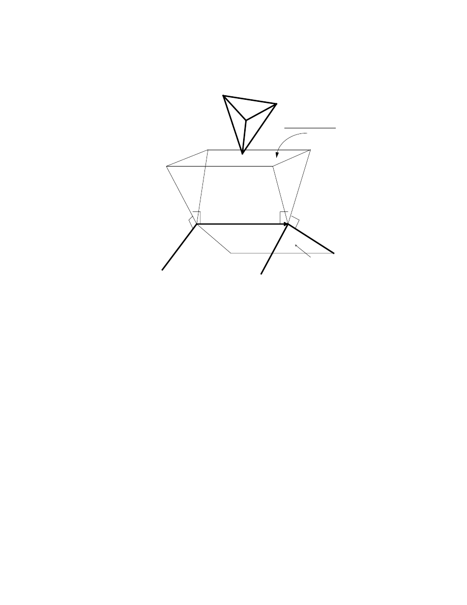
3.4 Vertex-Face Applicability Criterion
: : : : : : : : : : : : : : : : : : : 28
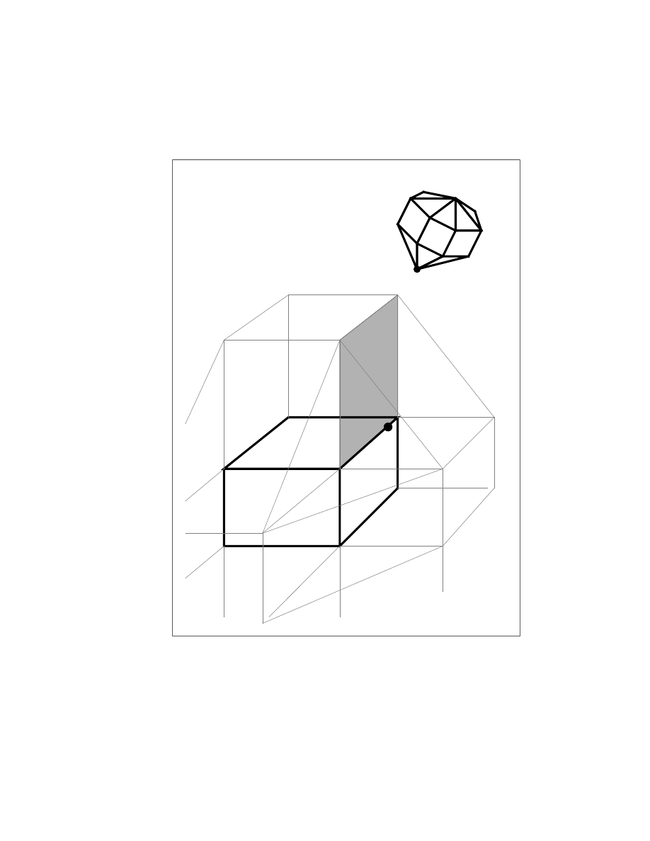
3.5 Preprocessing of a vertex's conical applicability region and a face's
cylindrical applicability region
: : : : : : : : : : : : : : : : : : : : : : 30
3.6 An example of Flared Voronoi Cells:
CP
F
corresponds to the ared
constraint place
CP of a face and CP
E
corresponds to the ared con-
straint plane
CP of an edge. R
0
1
and
R
0
2
are the
ared
Voronoi regions
of unperturbed
R
1
and
R
2
. Note that they overlap each other.
: : : : 31
3.7 (a) An overhead view of an edge lying above a face (b) A side view of
the face outward normal bounded by the two outward normals of the
edge's left and right faces.
: : : : : : : : : : : : : : : : : : : : : : : : 35
3.8 A Side View for Point-Vertex Applicability Criterion Proof
: : : : : : 43
3.9 An Overhead View for Point-Edge Applicability Criterion Proof
: : : 44
3.10 A Side View for Point-Edge Applicability Criterion Proof
: : : : : : : 44
3.11 A Side View for Point-Face Applicability Criterion Proof
: : : : : : : 45
3.12 Computation time vs. total no. of vertices
: : : : : : : : : : : : : : : 53
3.13 Polytopes Used in Example Computations
: : : : : : : : : : : : : : : 55
4.1 An example of sub-part hierarchy tree
: : : : : : : : : : : : : : : : : 59
4.2 An example for non-convex objects
: : : : : : : : : : : : : : : : : : : 63
4.3 Tangential intersection and boundary intersection between two Bezier
surfaces
: : : : : : : : : : : : : : : : : : : : : : : : : : : : : : : : : : 67
4.4 Closest features between two dierent orientations of a cylinder
: : : 71
4.5 Hierarchical representation of a torus composed of Bezier surfaces
: : 75

ix
6.1 A schematized 2-d conguration space and the partition of free space
into
x
1
-channels.
: : : : : : : : : : : : : : : : : : : : : : : : : : : : : 94
6.2 Two channels
C
1
and
C
2
joining the channel
C
3
, and a bridge curve in
C
3
.
: : : : : : : : : : : : : : : : : : : : : : : : : : : : : : : : : : : : : 96
6.3 A pictorial example of an inection point in
CS
R
vs. its view in
R
y at the slice x = x
0
: : : : : : : : : : : : : : : : : : : : : : : : : 103
6.4 An example of the algorithm in the 2-d workspace
: : : : : : : : : : : 105

1
Chapter 1
Introduction
The problem of collision detection or contact determination between two
or more objects is fundamental to computer animation, physical based modeling,
molecular modeling, computer simulated environments (e.g. virtual environments)
and robot motion planning as well [3, 7, 12, 20, 43, 45, 63, 69, 70, 72, 82, 85]. (De-
pending on the content of applications, it is also called with many dierent names,
such as interference detection, clash detection, intersection tests, etc.) In robotics,
an essential component of robot motion planning and collision avoidance is a geo-
metric reasoning system which can detect potential contacts and determine the exact
collision points between the robot manipulator and the obstacles in the workspace.
Although it doesn't provide a complete solution to the path planning and obstacle
avoidance problems, it often serves as a good indicator to steer the robot away from
its surrounding obstacles before an actual collision occurs.
Similarly, in computer animation, interactions among objects are simulated
by modeling the contact constraints and impact dynamics. Since prompt recognition
of possible impacts is a key to successful response to collisions in a timely fashion, a
simple yet ecient algorithm for collision detection is important for fast and realistic
animation and simulation of moving objects. The interference detection problem
has been considered one of the major bottlenecks in acheiving real-time dynamic
simulation.
Collision detection is also an integral part of many new, exciting technolog-

2
ical developments. Virtual prototyping systems create electronic representations of
mechanical parts, tools, and machines, which need to be tested for interconnectivity,
functionality, and reliability. The goal of these systems is to save processing and
manufacturing costs by avoiding the actual physical manufacture of prototypes. This
is similar to the goal of CAD tools for VLSI, except that virtual prototyping is more
demanding. It requires a complete test environment containing hundreds of parts,
whose complex interactions are based on physics and geometry. Collision detection
is vital component of such environments.
Another area of rising interests is synthetic environment, commonly known
as \virtual reality" (which is a comprehensiveterm promoting muchhypes and hopes).
In a synthetic environment, virtual objects (most of them stationary) are created and
placed in the world. A human participant may wish to move the virtual objects or
alter the scene. Such a simple action as touching and grasping involves geometric
contacts. A collision detection algorithm must be implemented to achieve any degree
of realism for such a basic motion. However, often there are hundreds, even thousands
of objects in the virtual world, a naive algorithm would probably take hours just to
check for possible interference whenever a human participant moves. This is not
acceptable for an interactive virtual environment. Therefore, a simple yet ecient
collision detection algorithm is almost indispensable to an interactive, realistic virtual
environment.
The objective of collision detection is to automatically report a geometric
contact when it is about to occur or has actually occurred. It is typically used in order
to simulate the physics of moving objects, or to provide the geometric information
which is needed in path planning for robots. The static collision detection problem
is often studied and then later extended to a dynamic environment. However, the
choice of step size can easily aect the outcome of the dynamic algorithms. If the
position and orientation of the objects is known in advance, the collision detection
can be solved as a function of time.
A related problem to collision detection is determining the minimum Eu-
clidean distance between two objects. The Euclidean distance between two objects
is a natural measurement of
proximity
for reasoning about their spatial relationship.

3
A dynamic solution to determining the minimum separation between two moving
objects can be a useful tool in solving the interference detection problem, since the
distance measurement provides all the necessary local geometric information and the
solution to the proximity question between two objects. However, it is not necessary
to determine the exact amount of separation or penetration between two objects to
decide whether a collision has taken place or not. That is, determining the minimum
separation or maximum penetration makes a much stronger statement than what
is necessary to answer the collision detection problem. But, this additional knowl-
edge can be extremely useful in computing the interaction forces and other penalty
functions in motion planning.
Collision detection is usually coupled with an appropriate response to the
collision. The collision response is generally application dependent and many algo-
rithms have been proposed for dierent environments like motion control in anima-
tion by Moore and Wilhelm [63], physical simulations by Bara, Hahn, Pentland and
Williams [3, 43, 70] or molecular modeling by Turk [85]. Since simplicity and ease of
implementation is considered as one of the important factors for any practical algo-
rithm in the computer graphics community, most collision detection algorithms used
for computer animation are rather simple but not necessary ecient. The simplest
algorithms for collision detection are based upon using bounding volumes and spatial
decomposition techniques. Typical examples of bounding volumes include cuboids,
spheres, octrees etc., and they are chosen due to the simplicity of nding collisions
between two such volumes. Once the two objects are in the vicinity of each other,
spatial decomposition techniques based on subdivision are used to solve the interfer-
ence problem. Recursive subdivision is robust but computationally expensive, and it
often requires substantially more memory. Furthermore the convergence to the solu-
tion corresponding to the contact point is linear. Repeating these steps at each time
instant makes the overall algorithm very slow. The run time impact of a subdivision
based collision detection algorithm on the physical simulation has been highlighted
by Hahn [43].
As interest in dynamic simulations has been rising in computer graphics
and robotics, collision detection has also received a great deal of attention. The im-

4
portance of collision detection extends to several areas like robot motion planning,
dynamic simulation, virtual reality applications and it has been extensively studied
in robotics, computational geometry, and computer graphics for more than a decade
[3, 4, 11, 13, 17, 41, 43, 45, 51, 53, 63]. Yet, there is no practical, ecient algo-
rithm available yet for general geometric models to perform collision detection in real
time. Recently, Pentland has listed collision detection as one of the major bottlenecks
towards real time virtual environment simulations [69].
In this thesis, we present an ecientalgorithm for collision detection between
objects with linear and curved boundaries, undergoing rigid motion. No assumption is
made on the motion of the object to be expressed as a closed form function of time. At
each instant, we only assume the knowledge of position and orientation with respect to
a global origin. We rst develop a fast, incremental distance computation algorithm
which keeps track of a pair of closest features between two convex polyhedra. The
expected running time of this algorithm is constant.
Next we will extend this incremental algorithm to non-convex objects by
using sub-part hierarchy tree representation and to curved objects by combining local
and global equation solving techniques. In addition, two methods are described to
reduce the frequency of interference detections by (1) a priority queue sorted by lower
bound on time to collisions (2) sweeping and sorting algorithms and a geometric
data structure. Some examples for applications of these algorithms are also briey
mentioned. The performance of these algorithms shows great promise for real-time
robotics simulation and computer animation.
1.1 Previous Work
Collision detection and the related problem of determining minimum dis-
tance has a long history. It has been considered in both static and dynamic (moving
objects) versions in [3], [11], [13], [17], [26], [27], [39], [40], [41], [65].
One of the earlier survey on \clash detection" was presented by Cameron
[12]. He mentioned three dierent approaches for dynamic collision detection. One of
them is to perform static collision detection repetitively at each discrete time steps,

5
but it is possible to miss a collision between time steps if the step size is too large.
Yet, it would be a waste of computation eort if the step size is too small. Another
method is to use a space-time approach: working directly in the four-dimensional sets
which form the abstract modes of the motion shapes (swept volumes in 4
D). Not
only is it dicult to visualize, but it is also a challenging task to model such sets,
especially when the motion is complex. The last method is to using sweeping volume
to represent moving objects over a period of time. This seems to be a rather intuitive
approach, but rather restrictive. Unless the motion of the objects are already known
in advance, it is impossible to sweep out the envelope of the moving objects and it
suppresses the temporal information. If two objects are both moving, the intersection
of two sweeping volume does not necessarily indicate an actual \clash" between two
objects.
Local properties have been used in the earlier motion planning algorithms
by Donald, Lozano-Perez and Wesley [28, 53] when two features come into contact.
In [53], Lozano-Perez and Wesley characterized the collision free motion planning
problem by using a point robot navigating in the conguration space by growing the
stationary obstacles with the size of the robot. As long as the point robot does not
enter a forbidden zone, a collision does not take place.
A fact that has often been overlooked is that collision
detection
for convex
polyhedra can be done in linear time in the worst case by Sancheti and Keerthi [77].
The proof is by reduction to linear programming. If two point sets have disjoint convex
hulls, then there is a plane which separates the two sets. Letting the four parameters of
the plane equations be variables, add a linear inequality for each vertex of polyhedron
A that species that the vertex is on one side of the plane, and an inequality for each
vertex of polyhedron B that species that it is on the other side. Megiddo and Dyers
work [30], [58], [59] showed that linear programming is solvable in linear time for any
xed number of variables. More recent work by Seidel [79] has shown that linear time
linear programming algorithms are quite practical for a small number of variables.
The algorithm of [79] has been implemented, and seems fast in practice.
Using linear-time preprocessing, Dobkin and Kirkpatrick were able to solve
the collision detection problem as well as compute the separation between two convex

6
polytopes in
O(log
j
A
j
log
j
B
j
) where A and B are polyhedra and
j
j
denotes the total
number of faces [27]. This approach uses a hierarchical description of the convex
objects and extension of their previous work [26]. This is one of the best known
theoretical bounds.
The capability of determining possible contacts in dynamic domains is im-
portant for computer animation of moving objects. We would like an animator to
perform impact determination by itself without high computational costs or much
coding eorts. Some algorithms (such as Boyse's [11] and Canny's [17]) solve the
problem in more generality than is necessary for computer animation; while others
do not easily produce the exact collision points and contact normal direction for col-
lision response [34]. In one of the earlier animation papers addressing the issue of
collision detection, Moore and Wilhelms [63] mentioned the method based on the
Cyrus-Beck clipping algorithm [74], which provides a simple, robust alternative but
runs in
O(n
2
m
2
) time for
m polyhedra and n vertices per polyhedron. The method
works by checking whether a point lies inside a polygon or polyhedron by using a inner
product calculation test. First, all vertices from polyhedron
B are tested against poly-
hedron
A, and then all vertices from A are tested for inclusion in B. This approach
along with special case treatments is reasonably reliable. But, the computation runs
in
O(n
2
) time where
n is the number of vertices per polyhedron.
Hahn [43] used a hierarchical method involving bounding boxes for intersec-
tion tests which run in
O(n
2
) time for each pair of polyhedra where
n is the number of
vertices for each polyhedron. The algorithm sweeps out the volume of bounding boxes
over a small time step to nd the exact contact locations. In testing for interference,
it takes every edge to check against each polygon and vice versa. Its performance is
comparable to Cyrus-Beck clipping algorithm. Our algorithm is a simple and ecient
method which runs in expected constant time for each pair of polyhedra, independent
of the geometric complexity of each polyhedron. (It would only take
O(m
2
) time for
m polyhedra with any number of vertices per polyhedron.) This provides a signicant
gain in speed for computer animation, especially for polyhedra with a large number
of vertices.
In applications involving dynamic simulations and physical motion, geomet-

7
ric coherence has been utilized to devise algorithms based on local features [3]. This
has signicantly improved the performance of collision detection algorithms in dy-
namic environments. Bara uses cached edges and faces to nd a separating plane
between two convex polytopes [3]. However, Bara's assumption to cache the last
\witnesses" does not hold when relative displacement of objects between successive
time steps are large and when closest features changes, it falls back on a global search;
while our method works fast even when there are relatively large displacements of ob-
jects and changes in closest features.
As for curved objects, Herzen and etc. [45] have described a general al-
gorithm based on time dependent parametric surfaces. It treats time as an extra
dimension and also assumes bounds on derivatives. The algorithm uses subdivision
technique in the resulting space and can therefore be slow. A similar method us-
ing interval arithmetic and subdivision has been presented for collision detection by
Du [29]. Du has extended it to dynamic environments as well. However, for com-
monly used spline patches computing and representing the implicit representations
is computationally expensive as stated by Homann [46]. Both algorithms, [29, 46],
expect a closed form expression of motion as a function of time. In [70], Pentland and
Williams proposes using implicit functions to represent shape and the property of the
\inside-outside" functions for collision detection. Besides its restriction to implicits
only, this algorithm has a drawback in terms of robustness, as it uses point samples.
A detailed explanation of these problems are described in [29]. Bara has also pre-
sented an algorithm for nding closest points between two convex closed objects only
[3].
In the related problem of computing the minimum separation between two
objects, Gilbert and his collaborators computed the minimum distance between two
convex objects with an expected linear time algorithm and used it for collision de-
tection. Our work shares with [38], [39], and [41] the calculation and maintenance
of closest points during incremental motion. But whereas [38], [39], and [41] require
expected linear time to verify the closest points, we use the properties of convex sets
to reduce this check to constant time.
Cameron and Culley further discussed the problem of interpenetration and

8
provided the intersection measurement for the use in a penalty function for robot mo-
tion planning [13]. The classical non-linear programming approaches for this problem
are presented in [1] and [9]. More recently, Sancheti and Keerthi [77] discussed the
computation of proximity between two convex polytopes from a complexity view-
point, in which the use of quadratic programming is proposed as an alternative to
compute the separation and detection problem between two convex objects in
O(n)
time in a xed dimension
d, where n is the number of vertices of each polytopes.
In fact, these techniques are used by researchers Karel Zikan [91], Richard Mastro,
etc. at the Boeing Virtual Reality Research Laboratory as a mean of computing the
distance between two objects.
Meggido's result in [58] stated that we can solve the problem of minimiz-
ing a convex quadratic function, subject to linear constraints in
R
3
in linear time by
transforming the quadratic programming using an appropriate ane transformation
of
R
3
(found in constant time) to a linear programming problem. In [60], Megiddo
and Tamir have further shown that a large class of separable convex quadratic trans-
portation problems with a xed number of sources and separable convex quadratic
programming with nonnegativity constraints and a xed number of linear equality
constraints can be solved in linear time. Below, we will present a short description of
how we can reduce the distance computation problem using quadratic programming
to a linear programming problem and solve it in linear time.
The convex optimization problem of computing the distance between two
convex polyhedra
A and B by quadratic programming can be formulated as follows:
Minimize
k
v
k
2
=
k
q
,
p
k
2
,
s.t.
p
2
A, q
2
B
subject to
n
1
X
i
=1
i
p
i
=
p;
n
1
X
i
=1
i
= 1
;
i
0
n
2
X
j
=1
j
q
j
=
q = p + v;
n
2
X
j
=1
j
= 1
;
j
0
where
p
i
and
q
j
are vertices of
A and B respectively. The variables are p, v,
i
's and
j
's. There are (
n
1
+
n
2
+6) constraints:
n
1
and
n
2
linear constraints from solving
i
's
and
j
's and 3 linear constraints each from solving the
x;y;z
,
coordinates of
p and
v respectively. Since we also have the nonnegativity constraints for p and v, we can

9
displace both
A and B to ensure the coordinates of p
0 and to nd the solutions
of 8 systems of equations (in 8 octants) to verify that the constraints, the
x;y;z
,
coordinates of
v
0, are enforced as well. According to the result on separable
quadratic programming in [60], this QP problem can be solved in
O(n
1
+
n
2
) time.
Overall, no good collision detection algorithms or distance computation
methods are known for general geometric models. Moreover, most of the litera-
ture has focussed on collision detection and the separation problem between a pair of
objects as compared to handling environments with multiple object models.
1.2 Overview of the Thesis
Chapter 3 through 5 of this thesis deal with algorithms for collision detection,
while chapter 6 gives an application of the collision detection algorithms in robot
motion planning. We begin in Chapter 2 by describing the basic knowledge necessary
to follow the development of this thesis work. The core of the collision detection
algorithms lies in Chapter 3, where the incremental distance computation algorithm
is described. Since this method is especially tailored toward convex polyhedra, its
extension toward non-convex polytopes and the objects with curved boundaries is
described in Chapter 4. Chapter 5 gives a treatment on reducing the frequency of
collision checks in a large environment where there may be thousands of objects
present. Chapter 6 is more or less self contained, and describes an opportunistic
global path planner which uses the techniques described in Chapter 3 to construct a
one-dimensional skeleton for the purpose of robot motion planning.
Chapter 2 described some computational geometry and modeling concepts
which leads to the development of the algorithms presented in this thesis, as well as
the object modeling to the input of our algorithms described in this thesis.
Chapter 3 contains the main result of thesis, which is a simple and fast
algorithm to compute the distance between two polyhedra by nding the closest fea-
tures between two convex polyhedra. It utilizes the geometry of polyhedra to establish
some local applicability criteria for verifying the closest features, with a preprocessing
procedure to reduce each feature's neighbors to a constant size, and thus guarantees

10
expected constant running time for each test. Data from numerous experimentstested
on a broad set of convex polyhedra in
R
3
show that the expected running time is
con-
stant
for nding closest features when the closest features from the previous time step
are known. It is linear in total number of features if no special initialization is done.
This technique can be used for dynamic collision detection, physical simulation, plan-
ning in three-dimensional space, and other robotics problems. It forms the heart of
the motion planning algorithm described in Chapter 6.
In Chapter 4, we will discuss how we can use the incremental distance com-
putation algorithm in Chapter 3 for dynamic collision detection between non-convex
polytopes and objects with curved boundary. Since the incremental distance com-
putation algorithm is designed based upon the properties of convex sets, extension
to non-convex polytopes using a sub-part hierarchical tree representation will be de-
scribed in detail here. The later part of this chapter deals with contact determination
between geometric models described by curved boundaries and undergoing rigid mo-
tion. The set of models include surfaces described by rational spline patches or piece-
wise algebraic functions. In contrast to previous approaches, we utilize the expected
constant time algorithm for tracking the closest features between convex polytopes
described in Chapter 3 and local numerical methods to extend the incremental nature
to convex curved objects. This approach preserves the coherence between successive
motions and exploits the locality in updating their possible contact status. We use
local and global algebraic methods for solving polynomial equations and the geomet-
ric formulation of the problem to devise ecient algorithms for non-convex curved
objects as well, and to determinethe exact contact points when collisions occur. Parts
of this chapter represent joint work with Dinesh Manocha of the University of North
Carolina at Chapel Hill.
Chapter 5 complements the previous chapters by describing two methods
which further reduce the frequency of collision checks in an environmentwith multiple
objects moving around. One assumes the knowledge of maximum acceleration and
velocity to establish a priority queue sorted by the lower bound on time to collision.
The other purely exploits the spatial arrangement without any other information
to reduce the number of pairwise interference tests. The rational behind this work

11
comes from the fact that though each pairwise interference test only takes expected
constant time, to check for all possible contacts among
n objects at all time can be
quite time consuming, especially if
n is in the range of hundreds or thousands. This
n
2
factor in the collision detection computation will dominate the run time, once
n
increases. Therefore, it is essential to come up with either heuristic approaches or
good theoretical algorithms to reduce the
n
2
pairwise comparisons.
Chapter 6 is independent of the other chapters of the thesis, and presents
a new robot path planning algorithm that constructs a global skeleton of free-space
by the incremental local method described in Chapter 3. The curves of the skeleton
are the loci of maxima of an articial potential eld that is directly proportional to
distance of the robot from obstacles. This method has the advantage of fast conver-
gence of local methods in uncluttered environments, but it also has a deterministic
and ecient method of escaping local extremal points of the potential function. We
rst describe a general roadmap algorithm, for conguration spaces of any dimension,
and then describe specic applications of the algorithm for robots with two and three
degrees of freedom.

12
Chapter 2
Background
In this chapter, we will describe some modeling and computational geome-
try concepts which leads to the development of the algorithms presented later in this
thesis, as well as the object modeling for the input to our collision detection algo-
rithms. Some of the materials presented in this chapter can be found in the books by
Homann, Preparata and Shamos [46, 71].
The set of models we used include rigid polyhedra and objects with surfaces
described by rational spline or piecewise algebraic functions. No deformation of the
objects is assumed under motion or external forces. (This may seem a restrictive
constraint. However, in general this assumption yields very satisfactory results, unless
the object nature is exible and deformable.)
2.1 Basic Concenpts
We will rst review some of the basic concepts and terminologies which are
essential to the later development of this thesis work.
2.1.1 Model Representations
In solid and geometricmodeling, there are two majorrepresentations schemata:
B-rep (boundary representation) and CSG (constructive solid geometry). Each has

13
its own advantages and inherent problems.
Boundary Representation:
to represent a solid object by describing its surface,
such that we have the complete information about the interior and exterior of an
object. This representation gives us two types of description: (a) geometric { the
parameters needed to describe a face, an edge, and a vertex; (b) topological { the
adjacencies and incidences of vertices, edges, and faces. This representation evolves
from the description for polyhedra.
Constructive Solid Geometry:
to represent a solid object by a set-theoretic
Boolean expression of
primitive
objects. The CSG operations include rotation, trans-
lation,
regularized union
,
regularized intersection
and
regularized dierence
. The CSG
standard primitives are the sphere, the cylinder, the cone, the parallelepiped, the tri-
angular prism, and the torus. To create a primitive part, the user needs to specify
the dimensions (such as the height, width, and length of a block) of these primitives.
Each object has a
local coordinate frame
associated with it. The conguration of each
object is expressed by the basic CSG operations (i.e. rotation and translation) to
place each object with respect to a global
world coordinate frame
.
Due to the nature of the distance computation algorithm for convex poly-
topes (presented in Chapter 3), which utilizes the adjacencies and incidences of fea-
tures as well as the geometric information to describe the geometric embedding re-
lationship, we have chosen the (modied) boundary representation to describe each
polyhedron (described in the next section). However, the basic concept of CSG rep-
resentation is used in constructing the subpart hierarchical tree to describe the non-
convex polyhedral objects, since each convex piece encloses a volume (can be thought
of as an object primitive).

14
2.1.2 Data Structures and Basic Terminology
Given the two major dierent representation schema, next we will describe
the modied
boundary
representation, which we use to represent convex polytope in
our algorithm, as well as some basic terminologies describing the geometric relation-
ship between geometric entities.
Let
A be a polytope. A is partitioned into features f
1
;:::;f
n
where
n is
the total number of features, i.e. n = f + e + v where f, e, v stands for the total
number of faces, edges, vertices respectively. Each feature (except vertex) is an open
subset of an ane plane and does not contain its boundary. This implies the following
relationships:
[
f
i
=
A;i = 1;:::;n
f
i
\
f
j
=
;
;i
6
=
j
Denition:
B is in the
boundary
of
F and F is in
coboundary
of
B, if and only if B
is in the closure of
F, i.e. B
F and B has one fewer dimension than F does.
For example, the coboundary of a vertex is the set of edges touching it and
the coboundary of an edge is the two faces adjacent to it. The boundary of a face is
the set of edges in the closure of the face.
We also adapt the winged edge representation. For those readers who are
not familiar with this terminology, please refer to [46]. Here we give a brief description
of the winged edge representation:
The edge is oriented by giving two incident vertices (the head and tail).
The edge points from tail to head. It has two adjacent faces cobounding it as well.
Looking from the the tail end toward the head, the adjacent face lying to the right
hand side is what we called the \right face" and similarly for the \left face" (please
see Fig.2.1).
Each polyhedron data structure has a eld for its features (faces, edges,
vertices) and Voronoi cells described below in Sec 2.1.4. Each feature (a vertex, an
edge, or a face) is described by its geometric parameters. Its data structure also
includes a list of its boundary, coboundary, and
Voronoi regions
(dened later in
Sec 2.1.4).

15
H
E
T
E
Right
Face
Left
Face
E
Figure 2.1: A winged edge representation
In addition, we will use the word \above" and \beneath" to describe the
relationship between a point and a face. In the homogeneous representation where
a point
P is presented as a vector (P
x
;P
y
;P
z
;1) and F's normalized unit outward
normal
N
F
is presented as vector (
a;b;c;
,
d), where
,
d is the directional distance
from the origin and the vector
n = (a;b;c) has the magnitude of 1. The plane which
F lies on is described by the plane equation ax + by + cz + d = 0.
A point P is
above
F
,
P
N
F
> 0
A point P is
on
F
,
P
N
F
= 0
A point P is
beneath
F
,
P
N
F
< 0
So, if
,
d > 0, then the origin lies
,
d units beneath the face F and vice versa.
Similarly, let
~e be the vector representing an edge E. Let H
E
= (
H
x
;H
y
;H
z
) and
T
E
= (
T
x
;T
y
;T
z
).
~e = H
E
,
T
E
= (
H
x
,
T
x
;H
y
,
T
y
;H
z
,
T
Z
;0) where H
E
and
T
E
are the head and tail of the edge
E respectively.
An edge E points
into
a face
F
,
~e
N
F
< 0
An edge E is
parallel
to a face
F
,
~e
N
F
= 0
An edge E points
out
of a face
F
,
~e
N
F
> 0

16
2.1.3 Voronoi Diagram
The proximity problem, i.e. \given a set
S of N points in
R
2
, for each point
p
i
2
S what is the set of points (x;y) in the plane that are closer to p
i
than to any
other point in
S ?", is often answered by the retraction approach in computational
geometry. This approach is commonly known as constructing the
Voronoi diagram
of the point set
S. This is an important concept which we will revisit in Chapter 3.
Here we will give a brief denition of Voronoi diagram.
The intuition to solve the proximity problem in
R
2
is to partition the plane
into regions, each of these is the set of the points which are closer to a point
p
i
2
S
than any other. If we know this partitioning, then we can solve the problem of
proximity directly by a simple query. The partition is based on the set of closest
points, e.g. bisectors which have 2 or 3 closest points.
Given two points
p
i
and
p
j
, the set of points closer to
p
i
than to
p
j
is just the
half-plane
H
i
(
p
i
;p
j
) containing
p
i
.
H
i
(
p
i
;p
j
) is dened by the perpendicular bisector
to
p
i
p
j
. The set of points closer to
p
i
than to any other point is formed by the
intersection of at most
N
,
1 half-planes, where
N is the number of points in the set
S. This set of points, V
i
, is called the
Voronoi polygon associated with
p
i
.
The collection of
N Voronoi polygons given the N points in the set S is
the
Voronoi diagram
,
V or(S), of the point set S. Every point (x;y) in the plane lies
within a Voronoi polygon. If a point (
x;y)
2
V (i), then p
i
is a
nearest point
to the
point (
x;y). Therefore, the Voronoi diagram contains all the information necessary
to solve the proximity problems given a set of points in
R
2
. A similar idea applies to
the same problem in three-dimensional or higher dimensional space [15, 32].
The extension of the Voronoi diagram to higher dimensional
features
(instead
of points) is called the generalized Voronoi diagram, i.e. the set of points closest to
a
feature
, e.g. that of a polyhedron. In general, the generalized Voronoi diagram
has quadratic surface boundaries in it. However, if the objects are convex, then the
generalized Voronoi diagram has planar boundaries. This leads to the denition of
Voronoi regions
which will be described next in Sec 2.1.4.

17
2.1.4 Voronoi Region
A
Voronoi region
associated with a
feature
is a set of points exterior to the
polyhedron which are closer to that feature than any other. The Voronoi regions
form a partition of space outside the polyhedron according to the closest feature.
The collection of Voronoi regions of each polyhedron is the Voronoi diagram of the
polyhedron. Note that the Voronoi diagram of a convex polyhedron has linear size
and consists of polyhedral regions. A
cell
is the data structure for a Voronoi region.
It has a set of constraint planes which bound the Voronoi region with pointers to the
neighboring cells (which share a constraint plane with it) in its data structure. If a
point lies on a constraint plane, then it is equi-distant from the two features which
share this constraint plane in their Voronoi regions.
Using the geometric properties of convex sets, applicability criteria (ex-
plained in Sec.3.2) are established based upon the Voronoi regions. If a point
P
on object
A lies inside the Voronoi region of f
B
on object
B, then f
B
is a closest
feature to the point
P. (More details will be presented in Chapter 3.)
In Chapter 3, we will describe our incremental distance computation al-
gorithm which utilizes the concept of Voronoi regions and the properties of convex
polyhedra to perform collision detection in expected constant time. After giving the
details of polyhedral model representations, in the next section we will describe more
general object modeling to include the class of non-polyhedral objects as well, with
emphasis on curved surfaces.
2.2 Object Modeling
The set of objects we consider, besides convex polytopes, includes non-
convex objects (like a torus) as well as two dimensional manifolds described using
polynomials. The class of parametric and implicit surfaces described in terms of
piecewise polynomial equations is currently considered the state of the art for mod-
eling applications [35, 46]. These include free-form surfaces described using spline
patches, primitive objects like polyhedra, quadrics surfaces (like cones, ellipsoids),

18
torus and their combinations obtained using CSG operations. For arbitrary curved
objects it is possible to obtain reasonably good approximations using B-splines
Most of the earlier animation and simulation systems are restricted to poly-
hedral models. However,modeling with surfaces bounded by linear boundaries poses a
serious restriction in these systems. Our contact determination algorithms for curved
objects are applicable on objects described using spline representations (Bezier and
B-spline patches) and algebraic surfaces. These representations can be used as prim-
itives for CSG operations as well.
Typically spline patches are described geometrically by their control points,
knot vectors and order continuity [35]. The control points have the property that the
entire patch lies in the convex hull of these points. The spline patches are represented
as piecewise Bezier patches. Although these models are described geometrically using
control polytopes, we assume that the Bezier surface has an algebraic formulation in
homogeneous coordinates as:
F
(
s;t) = (X(s;t);Y (s;t);Z(s;t);W(s;t)):
(2
:1)
We also allow the objects to be described implicitly as algebraic surfaces. For exam-
ples, the quadric surfaces like spheres, cylinders can be simply described as a degree
two algebraic surface. The algebraic surfaces are represented as
f(x;y;z) = 0.
2.2.1 Motion Description
All objects are dened with respect to a global coordinate system, the
world
coordinate frame
. The initial conguration is specied in terms of the origin of the
system. As the objects undergo rigid motion, we update their positions using a 4
4
matrix,
M, used to represent the rotation as well as translational components of the
motion (with respect to the origin). The collision detection algorithm is based only
on local features of the polyhedra (or control polytope of spline patches) and does not
require the position of the other features to be updated for the purpose of collision
detection at every instant.

19
2.2.2 System of Algebraic Equations
Our algorithm for collision detection for algebraic surface formulates the
problem of nding closest points between object models and contact determination
in terms of solving a system of algebraic equations. For most instances, we obtain a
zero dimensional algebraic system consisting of
n equations in n unknowns. However
at times, we may have an overconstrained system, where the number of equations is
more than the number of unknowns or an underconstrained system, which has innite
number of solutions. We will be using algorithms for solving zero dimensional systems
and address how they can be modied to other cases. In particular, we are given a
system of
n algebraic equations in n unknowns:
F
1
(
x
1
;x
2
;:::;x
n
) = 0
...
(2.2)
F
n
(
x
1
;x
2
;:::;x
n
) = 0
Let their degrees be
d
1
,
d
2
,
:::, d
n
, respectively. We are interested in computing all
the solutions in some domain (like all the real solutions to the given system).
Current algorithms for solving polynomial equations can be classied into
local and global methods. Local methods like Newton's method or optimization
routines need good initial guesses to each solution in the given domain. Their perfor-
mance is a function of the initial guesses. If we are interested in computing all the real
solutions of a system of polynomials, solving equations by local methods requires that
we know the number of real solutions to the system of equations and good guesses to
these solutions.
The global approaches do not need any initial guesses. They are based on
algebraic approaches like resultants, Gr}obner bases or purely numerical techniques
like the homotopy methods and interval arithmetic. Purely symbolic methods based
on resultants and Gr}obner bases are rather slow in practice and require multiprecision
arithmetic for accurate computations. In the context of nite precision arithmetic,
the main approaches are based on resultant and matrix computations [55], continua-

20
tion methods [64] and interval arithmetic [29, 81]. The recently developed algorithm
based on resultants and matrix computations has been shown to be very fast and
accurate on many geometric problems and is reasonably simple to implement using
linear algebra routines by Manocha [55]. In particular, given a polynomial system
the algorithm in [55] reduces the problem of root nding to an eigenvalue problem.
Based on the eigenvalue and eigenvectors, all the solutions of the original system are
computed. For large systems the matrix tends to be sparse. The order of the matrix,
say
N, is a function of the algebraic complexity of the system. This is bounded by
the Bezout bound of the given system corresponding to the product of the degrees of
the equations. In most applications, the equations are sparse and therefore, the order
of the resulting matrix is much lower than the Bezout bound. Good algorithms are
available for computing the eigenvalues and eigenvectors of a matrix. Their running
time can be as high as
O(N
3
). However, in our applications we are only interested
in a few solutions to the given system of equations in a corresponding domain, i.e.
real eigenvalues. This corresponds to nding selected eigenvalues of the matrix corre-
sponding to the domain. Algorithms combining this with the sparsity of the matrix
are presented in [56] and they work very well in practice.
The global root nders are used in the preprocessing stage. As the objects
undergo motion, the problem of collision detection and contact determination is posed
in terms of a new algebraic system. However, the new algebraic system is obtained
by a slight change in the coecients of the previous system of equations. The change
in coecients is a function of the motion between successive instances and this is
typically small due to temporal and spatial coherence. Since the roots of an algebraic
system are a continuous function of the coecients, the roots change slightly as well.
As a result, the new set of roots can be computed using local methods only. We can
either use Newton's method to compute the roots of the new set of algebraic equations
or inverse power iterations [42] to compute the eigenvalues of the new matrix obtained
using resultant formulation.

21
Chapter 3
An Incremental Distance
Computation Algorithm
In this chapter we present a simple and ecient method to compute the
distance between two convex polyhedra by nding and tracking the closest points.
The method is generally applicable, but is especially well suited to repetitive distance
calculation as the objects move in a sequence of small, discrete steps due to its
incremental nature. The method works by nding and maintaining a pair of closest
features (vertex, edge, or face) on the two polyhedra as the they move. We take
advantage of the fact that the closest features change only infrequently as the objects
move along nely discretized paths. By preprocessing the polyhedra, we can verify
that the closest features have not changed or performed an update to a neighboring
feature in expected constant time. Our experiments show that, once initialized, the
expected running time of our incremental algorithm is
constant
independent of the
complexity of the polyhedra, provided the motion is not abruptly large.
Our method is very straightforward in its conception. We start with a
candidate pair of features, one from each polyhedron, and check whether the closest
points lie on these features. Since the objects are convex, this is a local test involving
only the neighboring features (boundary and coboundary as dened in Sec. 2.1.2) of
the candidate features. If the features fail the test, we step to a neighboring feature
of one or both candidates, and try again. With some simple preprocessing, we can

22
guarantee that every feature has a constant number of neighboring features. This is
how we can verify a closest feature pair in expected constant time.
When a pair of features fails the test, the new pair we choose is guaranteed
to be closer than the old one. Usually when the objects move and one of the closest
features changes, we can nd it after a single iteration. Even if the closest features
are changing rapidly, say once per step along the path, our algorithm will take only
slightly longer. It is also clear that in any situation the algorithm must terminate in
a number of steps at most equal to the number of feature pairs.
This algorithm is a key part of our general planning algorithm, described
in Chap.6 That algorithm creates a one-dimensional roadmap of the free space of
a robot by tracing out curves of maximal clearance from obstacles. We use the
algorithm in this chapter to compute distances and closest points. From there we can
easily compute gradients of the distance function in conguration space, and thereby
nd the direction of the maximal clearance curves.
In addition, this technique is well adapted for dynamic collision detection.
This follows naturally from the fact that two objects collide if and only if the distance
between them is less than or equal to zero (plus some user dened tolerance). In fact,
our approach provide more geometric information than what is necessary, i.e. the
distance information and the closest feature pair may be used to compute inter-object
forces.
3.1 Closest Feature Pair
Each object is represented as a convex polyhedron, or a union of convex
polyhedra. Many real-world objects that have curved surfaces are represented by
polyhedral approximations. The accuracy of the approximations can be improved by
increasing the resolution or the number of vertices. With our method, there is little
or no degradation in performance when the resolution is increased in the convex case.
For nonconvex objects, we rely on subdivision into convex pieces, which unfortunately,
may take
O((n+r
2
)
logr) time to partition a nondegenerate simple polytope of genus
0, where
n is the number of vertices and r is the number of
reex edges
of the original

23
nonconvex object [23, 2]. In general, a polytope of
n verticescan always be partitioned
into
O(n
2
) convex pieces [22].
Given the object representation and data structure for convex polyhedra
described in Chapter 2, here we will dene the term
closest feature pair
which we
quote frequently in our description of the distance computation algorithm for convex
polyhedra.
The closest pair of features between two general convex polyhedra is dened
as the pair of features which contain the closest points. Let polytopes
A and B denote
the convex sets in
R
3
. Assume
A and B are closed and bounded, therefore, compact.
The distance between objects
A and B is the shortest Euclidean distance d
AB
:
d
AB
= inf
p
2
A;q
2
B
j
p
,
q
j
and let
P
A
2
A, P
B
2
B be such that
d
AB
=
j
P
A
,
P
B
j
then
P
A
and
P
B
are a pair of closest points between objects
A and B.
For each pair of features (
f
A
and
f
B
) from objects A and B, rst we nd the
pair of nearest points (say
P
A
and
P
B
) between these
two features
. Then, we check
whether these points are a pair of closest points
between
A
and
B. That is, we need
to verify that
f
B
is truly a closest feature on
B to P
A
and
f
A
is truly a closest feature
on
A to P
B
This is verication of whether
P
A
lies inside the Voronoi region of
f
B
and whether
P
B
lies inside the Voronoi region of
f
A
(please see Fig. 3.1). If either
check fails, a new (closer) feature is substituted, and the new pair is checked again.
Eventually, we must terminate with a closest pair, since the distance between each
candidate feature pair decreases, as the algorithm steps through them.
The test of whether one point lies inside of a Voronoi region of a feature
is what we call an \applicability test". In the next section three intuitive geometric
applicability tests, which are the essential components of our algorithm, will be de-
scribed. The overall description of our approach and the completeness proof will be
presented in more detail in the following sections.
24
R
1
R
2
F
a
CP
Object B
Object A
V
b
Pa
E
a
(a)
Figure 3.1: Applicability Test: (
F
a
;V
b
)
!
(
E
a
;V
b
) since
V
b
fails the applicability test
imposed by the constraint plane
CP. R
1
and
R
2
are the Voronoi regions of
F
a
and
E
a
respectively.

25
3.2 Applicability Criteria
There are three basic applicability criteria which we use throughout our
distance computation algorithm. These are (i) point-vertex, (ii) point-edge, and (iii)
point-face applicability conditions. Each of these applicability criteria is equivalent
to a membership test which veries whether
the point
lies in the Voronoi region of
the
feature
. If the
nearest points
on two features both lie inside the Voronoi region of
the other feature, then the two features are a closest feature pair and the points are
closest points between the polyhedra.
3.2.1 Point-Vertex Applicability Criterion
If a vertex
V of polyhedron B is truly a closest feature to point P on polyhe-
dron
A, then P must lie within the Voronoi region bounded by the constraint planes
which are perpendicular to the coboundary of
V (the edges touching V ). This can be
seen from Fig.3.2. If
P lies outside the region dened by the constraint planes and
hence on the other side of one of the constraint planes, then this implies that there
is at least one edge of
V 's coboundary closer to P than V . This edge is normal to
the violated constraint. Therefore, the procedure will walk to the corresponding edge
and iteratively call the closest feature test to verify whether the
feature containing
P
and the
new edge
are the closest features on the two polyhedra.
3.2.2 Point-Edge Applicability Criterion
As for the point-edge case, if edge
E of polyhedron B is really a closest
feature to the point
P of polyhedron A, then P must lie within the Voronoi region
bounded by the four constraint planes of
E as shown in Fig.3.3. Let the head and
tail of
E be H
E
and
T
E
respectively. Two of these planes are perpendicular to
E
passing through the head
H
E
and the tail
T
E
of
E. The other two planes contain E
and one of the normals to the coboundaries of
E (i.e. the right and the left faces of
E). If P lies inside this wedge-shaped Voronoi region, the applicability test succeeds.
If
P fails the test imposed by H
E
(or
T
E
), then the procedure will walk to
H
E
(or

26
V
ObjectB
P
ObjectA
Voronoi Region
Figure 3.2: Point-Vertex Applicability Criterion
T
E
) which must be closer to
P and recursively call the general algorithm to verify
whether the
new vertex
and the
feature containing
P are the two closest features on
two polyhedra respectively. If
P fails the applicability test imposed by the right (or
left) face, then the procedure will walk to the right (or left) face in the coboundary
of
E and call the general algorithm recursively to verify whether the
new face
(the
right or left face of
E) and the
feature containing
P are a pair of closest features.
3.2.3 Point-Face Applicability Criterion
Similarly, if a face
F of polyhedron B is actually a closest feature to P on
polyhedron
A, then P must lie within F's Voronoi region dened by F's prism and
above the plane containing
F, as shown in Fig.3.4. F's
prism
is the region bounded
by the constraint planes which are perpendicular to
F and contain the edges in the
boundary of
F.
First of all, the algorithm checks if
P passes the applicability constraints
imposed by
F's edges in its coboundary. If so, the feature containing P and F
27
E
T
e
H
e
Right-Face
P
Left-Face
ObjectA
Voronoi Region
Figure 3.3: Point-Edge Applicability Criterion
are a pair of closest features; else, the procedure will once again walk to the edge
corresponding to a failed constraint check and call the general algorithm to check
whether the
new edge
in
F's boundary (i.e. E
F
) and the
feature containing
P are a
pair of the closest features.
Next, we need to check whether
P lies above F to guarantee that P is not
inside the polyhedron
B. If P lies beneath F, it implies that there is at least one
feature on polyhedron
B closer to the feature containing P than F or that collision
is possible. In such a case, the nearest points on
F and the feature containing P may
dene a local minimum of distance, and stepping to a neighboring feature of
F may
increase the distance. Therefore, the procedure will call upon a
O(n) routine (where
n is the number of features of B) to search for the closest feature on the polyhedron
B to the feature containing P and proceed with the general algorithm.

28
N
F
2
F
P
F
Voronoi Region
ObjectA
Figure 3.4: Vertex-Face Applicability Criterion
3.2.4 Subdivision Procedure
For vertices of typical convex polyhedra, there are usually three to six edges
in the coboundary. Faces of typical polyhedra also have three to six edges in the
boundaries. Therefore, frequently the applicability criteria require only a few quick
tests for each round. When a face has more than ve edges in its boundary or when a
vertex has more than ve edges in its coboundary, the Voronoi region associated with
each feature is preprocessed by subdividing the whole region into smaller cells. That
is, we subdivide the prismatic Voronoi region of a face (with more than ve edges)
into quadrilateral cells and divide the Voronoi region of a vertex (with more than ve
coboundaries) into pyrmidal cells. After subdivision, each Voronoi cell is dened by
4 or 5 constraint planes in its boundary or coboundary. Fig.3.5 shows how this can
be done on a vertex's Voronoi region with 8 constraint planes and a face's Voronoi
region with 8 constraint planes. This subdivision procedure is a simple algorithm
which can be done in linear time as part of preprocessing, and it guarantees that
when the algorithm starts, each Voronoi region has a constant number of constraint

29
planes. Consequently, the three applicability tests described above run in
constant
time
.
3.2.5 Implementation Issues
In order to minimize online computation time, we do all the subdivision
procedures and compute all the Voronoi regions rst in a one-time computational
eort. Therefore, as the algorithm steps through each iteration, all the applicabil-
ity tests would look uniformly alike | all as \point-cell applicability test", with a
slight dierence to the point-face applicability criterion. There will no longer be any
distinction among the three basic applicability criteria.
Each feature is an open subset of an ane plane. Therefore, end points
are not consider part of an edge. This is done to simplify the proof of convergence.
Though we use the winged edge representation for our implementation, all the edges
are not deliberately oriented as in the winged edge representation.
We also use hysteresis to avoid cycling in degenerate cases when there is more
than one feature pair separated at approximately the same distance. We achieve this
by making the Voronoi regions overlap each other with small and \ared" displace-
ments. To illustrate the \ared Voronoi cells", we demonstrate them by an example
in Fig. 3.6. Note that all the constraint planes are tilted outward by a small angular
displacement as well as innitesimal translational displacement. The angular dis-
placement is used to ensure the overlap of adjacent regions. So, when a point falls on
the borderline case, it will not ip back and forth between the two adjacent Voronoi
regions. The small translational displacement in addition to angular displacement is
needed for numerical problem arising from point coordinate transformations. For an
example, if we transform a point
p by a homogeneous matrix T and transform it back
by
T
,1
, we will not get the same point
p but p
0
with small dierences in each of its
coordinate, i.e.
T
,1
(
Tp)=neqp.
All faces are convex,
but
because of subdivision they can be coplanar. Where
the faces are coplanar, the Voronoi regions of the edges between them is null and face
constraints point directly to the next Voronoi region associated with their neighboring
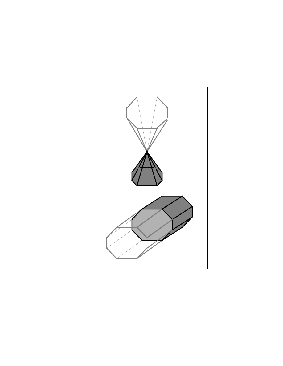
30
R
1
R
2
R
3
R
5
R
6
R
4
V
a
F
b
Object A
Object B
(b)
R
b
R
a
Figure 3.5: Preprocessing of a vertex's conical applicability region and a face's cylin-
drical applicability region

31
CP
E
R
1
’
CP
F
CP
R
2
’
R
2
R
1
Object A
Figure 3.6: An example of Flared Voronoi Cells:
CP
F
corresponds to the ared
constraint place
CP of a face and CP
E
corresponds to the ared constraint plane
CP of an edge. R
0
1
and
R
0
2
are the
ared
Voronoi regions of unperturbed
R
1
and
R
2
.
Note that they overlap each other.

32
coplanar faces.
In addition, the order of the applicability test in each case does not aect
the nal result of the algorithm. However, to achieve faster convergence, we look for
the constraint plane which is violated the most and its associated neighboring feature
to continue the verication process in our implementation.
We can also calculate how frequently we need to check for collision by taking
into consideration the maximum magnitude of acceleration and velocity and initial
separation. We use a priority queue based on the lower bound on time to collision to
detect possible intersection at a timely fashion. Here the step size is adaptively set
according to the lower bound on time to collision we calculate. For more information
on this approach, please see Chapter 5 of this thesis.
In the next section, we will show how these applicability conditions are used
to
update
a pair of closest features between two convex polyhedra in expected
constant
time
.
3.3 The Algorithm
Given a pair of features, there are altogether 6 possible cases that we need
to consider: (1) a pair of vertices, (2) a vertex and an edge, (3) a vertex and a face,
(4) a pair of edges, (5) an edge and a face, and (6) two faces. In general, the case of
two faces or edge-face rarely happens. However, in applications such as path planning
we may end up moving along maximal clearance paths which keep two faces parallel,
or an edge parallel to a face. It is important to be able to detect when we have such
a degenerate case.
3.3.1 Description of the Overall Approach
Given a pair of features
f
A
and
f
B
each from convex polyhedra
A and B
respectively, except for cases (1), (5) and (6), we begin by computing the nearest
points between
f
A
and
f
B
. The details for computing these nearest points between
f
A
and
f
B
are rather trivial, thus omitted here (please refer to Appendix A if necessary).

33
However, we would like to reinforce one point. We do not assume innitely long
edges when we compute these nearest points. The nearest points computed given two
features are the actual points on the features, not some virtual points on innitely
extended edges, i.e. nearest points between edges may be their endpoints.
(1) If the features are a pair of vertices,
V
A
and
V
B
, then both
V
A
and
V
B
have to
satisfy the point-vertex applicability conditions imposed by each other, in order for
them to be the closest features. If
V
A
fails the point-vertex applicability test imposed
by
V
B
or vice versa, then the algorithm will return a new pair of features, say
V
A
and
E
B
(the edge whose corresponding constraint was violated in the point-vertex
applicability test), then continue verifying the new feature pair until it nds a closest
pair.
(2) Given a vertex
V
A
and an edge
E
B
from
A and B respectively, the algorithm will
check whether the vertex
V
A
satises the point-edge applicability conditions imposed
by the edge
E
B
and
whether the nearest point
P
E
on the edge
E
B
to
V
A
satises the
point-vertex applicability conditions imposed by the vertex
V
A
. If both checks return
\true", then
V
A
and
E
B
are the closest features. Otherwise, a corresponding new pair
of features (depending on which test failed) will be returned and the algorithm will
continue to walk closer and closer toward a pair of closest features.
(3) For the case of a vertex
V
A
and a face
F
B
, both of the point-face applicability tests
imposed by the face
F
B
to the vertex
V
A
and
the point-vertex applicability criterion
by
V
A
to the nearest point
P
F
on the face must be satised for this pair of features
to qualify as a closest-feature pair. Otherwise, a new pair of features will be returned
and the algorithm will be called again until the closest-feature pair is found.
(4) Similarly, given a pair of edges
E
A
and
E
B
as inputs, if their nearest points
P
A
and
P
B
satisfy the point-edge applicability criterion imposed by
E
B
and
E
A
, then
they are a pair of closest features between two polyhedra. If not, one of the edges
will be changed to a neighboring vertex or a face and the verication process will be
done again on the new pair of features.
(5) When a given pair of features is an edge
E
A
and a face
F
B
, we rst need to decide

34
whether the edge is parallel to the face. If it is not, then either one of two edge's
endpoints and the face,
or
the edge and some other edge bounding the face will be the
next candidate pair. The former case occurs when the head or tail of the edge satises
the point-face applicability condition imposed by the face, and when one endpoint of
E is closer to the plane containing F than the other endpoint of E. Otherwise, the
edge
E and the closest edge E
F
on the face's boundary to
E will be returned as the
next candidate features.
If the edge and the face are parallel, then they are the closest features
provided three conditions are met. (i) The edge must cut the \applicability prism"
Prism
F
which is the region bounded by the constraint planes perpendicular to
F
B
and passing through
F
B
's boundary (or the region swept out by
F
B
along its normal
direction), that is
E
\
Prism
F
6
=
;
(ii) the face normal must lie between the face
normals of the faces bounding the edge (see Fig. 3.7, Sec. 3.4, and the pseudo code in
Appendix B), (iii) the edge must lie above the face. There are several other situations
which may occur, please see Appendix B or the proof of completeness in Sec. 3.4 for
a detailed treatment of edge-face case.
(6) In the rare occasion when two faces
F
A
and
F
B
are given as inputs, the algorithm
rst has to decide if they are parallel. If they are, it will invoke an overlap-checking
subroutine which runs in linear time in the total number of edges of
F
A
and
F
B
.
(Note: it actually runs in constant time after we preprocess the polyhedra, since
now all the faces have constant size of boundaries.) If they are both parallel,
F
A
's
projection down onto the face
F
B
overlaps
F
B
and each face is above the other face
relative to their outward normals, then they are in fact the closest features.
But, if they are parallel yet not overlapping, then we use a linear time
procedure [71] to nd the closest pair of edges, say
E
A
and
E
B
between
F
A
and
F
B
,
then invoke the algorithm again with this new pair of candidates (
E
A
;E
B
).
If
F
A
and
F
B
are not parallel, then rst we nd the closest feature (either
a vertex or an edge)
f
A
of
F
A
to the plane containing
F
B
and vice versa. Then, we
check if this closest feature
f
A
satisfy the applicability constraint imposed by
F
B
.
If so, the new candidate pair will be this closest feature
f
A
and
F
B
; otherwise, we
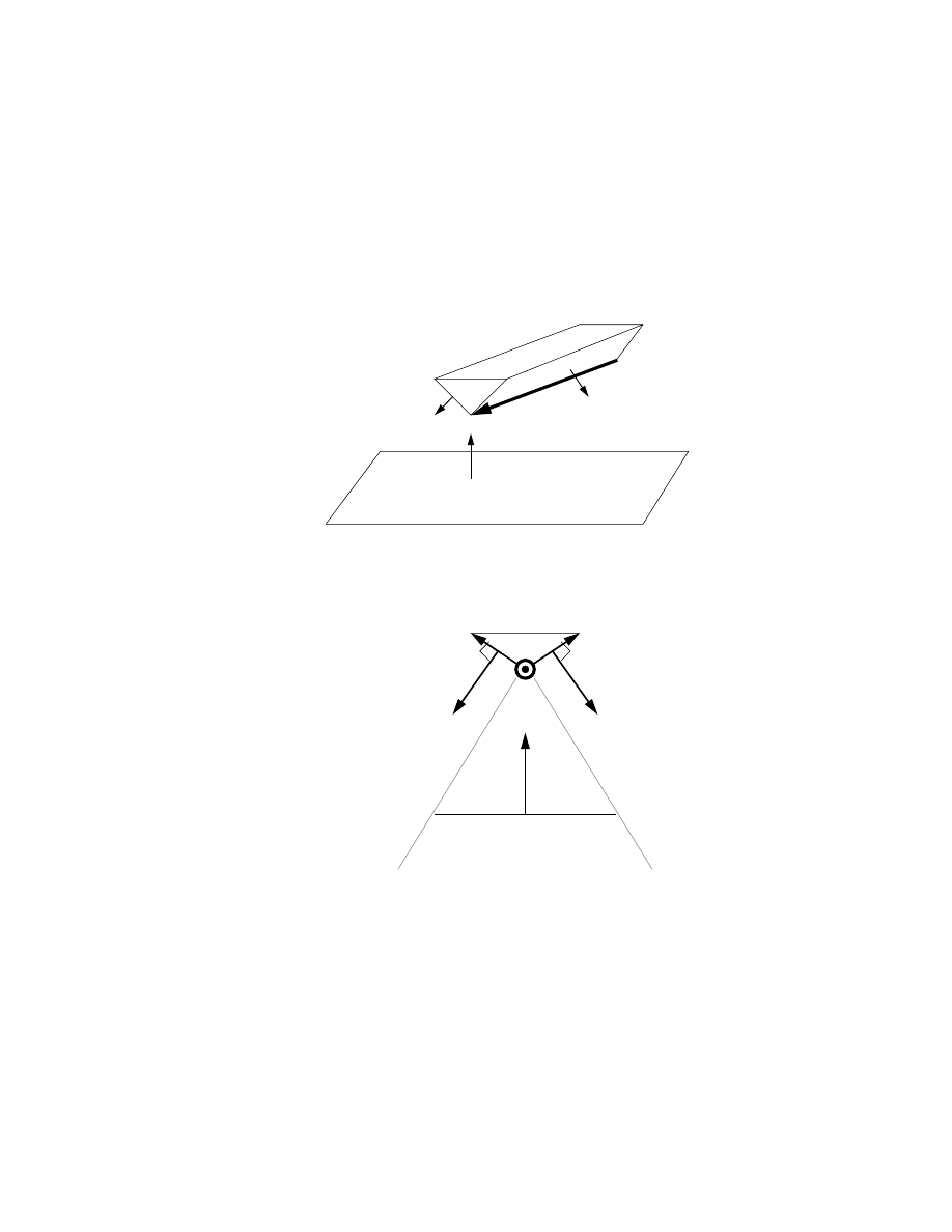
35
E
N
R
N
L
N
F
Object A
F
(a)
(b)
N
F
E
F
Object A
E x N
R
N
L
x E
P
R
N
L
P
L
N
R
Figure 3.7: (a) An overhead view of an edge lying above a face (b) A side view of
the face outward normal bounded by the two outward normals of the edge's left and
right faces.

36
enumerate over all edge-pairs between two faces to nd a closest pair of edges and
proceed from there.
If one face lies on the \far side" of the other (where the face is beneath the
other face relative to their face outward normals) or vice versa, then the algorithm
invokes a linear-time routine to step away from this local minimum of distance, and
provides a new pair of features much closer than the previous pair. Please refer to
Appendix B for a complete description of face-face case.
3.3.2 Geometric Subroutines
In this section, we will present some algorithms for geometric operations on
polytopes. They are used in our implementation of the algorithms described in this
thesis.
Edge & Face's Prism Intersection:
To test for the intersectionof a
parallel
edge
E
A
to
F
B
within a prism
Prism
F
swept out by a face
F
B
along its face normal direction
N
F
, we check whether portion
of this edge lies within the interior region of
Prism
F
. This region can be visualized
as the space bounded by
n planes which are perpendicular to the face F
B
and passing
through the
n edges in its boundary.
Suppose
F
i
is a face of the prismatic region
Prism
F
and perpendicular to the
face
F
B
and passing through the edge
E
i
bounding
F
B
. To test for
E
A
's intersection
within the prism
Prism
F
, we need to check whether
E
A
intersects some face
F
i
of
R
F
.
We can perform this test with easy and ecient implementation
1
of this
intersection test. We rst parameterize the edge
E
A
between 0 and
l where l is the
length of
E
A
. The idea is to intersect the intervals of the edge
E
A
contained in the
exterior
2
of each half-space with each constraint plane in the prism of a face
F
B
.
1
suggested by Brian Mirtich
2
We dene the exterior half-space of each constraint plane to be the half-space where all the points
satisfy the applicability constraints imposed by
F
B
's boundary. The "point-cell-checkp" routine in
the pseudo code can clarify all the ambiguity. Please refer to Appendix B if necessary.

37
First, we decide whether the edge
E
A
points inward or outward of each hyperplane
F
i
of the region by taking the inner product of
E
A
's unit directional vector with
F
i
's
outward normal
N
F
i
.
Then, we can decide which portion of
E
A
intersect the
exterior
half-space
of
F
i
by taking another inner product of the head of
E
A
and
F
i
's outward normal
normalized by the inner product of
E
A
and
N
F
i
to calculate the relative \inclusion"
factor of
E
A
inside of the prism region. The relative (beginning and ending) inclusion
factors should be in the range of 0 and
l for an indication of an edge-face's prism
intersection.
Pseudo code for this approach just described is listed in Appendix B. This
geometric test is used in our implementation of distance computation algorithm as a
subroutine to check whether a given edge intersects the Voronoi prism of a given face
to test their eligibilities be a pair of closest features.
Face & Face's Prisim Intersection:
To check if two convex polygons
A and B are overlapping, one of the basic
approaches is to verify if there is some vertex of
A lying on the \inside" of
all
edges in
the boundary of
B or vice versa. The \inside" refers to the
interior half-plane
of the
edge, not necessary the interior of the polygon. A n-sided convex polygon is formed
by the intersection of interior half-planes of
n edges. We can use the fact that two
polygons do no overlap if there exists a separating line passing through one edge in
the boundary of either face. The polygons overlap, if and only if
none
of the edges
in the boundary of both polygons forms a separating line.
For our own application, we are interested to verify whether a face
A's pro-
jection down to the plane containing the face
B overlaps with the face B, where A
and
B are
parallel
and in
R
3
. To nd a separating line between two such polygons
in
R
3
, we check if there exists a supporting plane passing through an edge in the
boundary of one polygon such that all vertices of the other polygon lies in the \exte-
rior half-space" of the supporting plane. The supporting plane is perpendicular the
polygon and containing an edge in the polygon's boundary. This approach runs in
O(N
2
) time where
N is the number of edges of each polygon.

38
An elegant approach which runs in
O(M + N) can be found in [66, 71],
where the two polygons
A and B each has M, N vertices respectively. This approach
not only determines whether two convex polygon intersect or not, it also nds the
intersections between them. The basic approach is to \advance" along the edges of
A and B to nd the \internal chain" of vertices which form the intersection polygon.
Please refer to [66, 71] for all the details.
3.3.3 Analysis of the Algorithm
A careful study of all of the above checks shows that they all take time in
proportion to the size of the boundary and coboundary of each feature. Therefore,
after subdivision preprocessing, all local tests run in constant time since each feature
now has constant number of neighboring features. The only exception to this is when
f
A
is a face, and
f
B
lies under the plane containing
f
A
(or vise versa). In this case,
we can not use a local feature change, because this may lead to the procedure getting
stuck in a loop. Geometrically, we are moving around the local minimum of the
distance function, in which we may become trapped. When this situation occurs, we
search among all the features of object
A to nd a closest feature to the f
B
3
. This is
not a constant time step, but note that it is impossible for the algorithm to move to
such an opposing face once it is initialized and given a reasonable step size (not more
than a few degrees of rotation). So this situation can only occur when the algorithm
is rst called on an arbitrary pair of features.
The algorithm can take any arbitrary pair of features of two polyhedra and
nd a true pair of closest features by iteratively checking and changing features. In
this case, the running time is proportional to the number of feature pairs traversed
in this process. It is not more than the product of the numbers of features of the two
polyhedra, because the distance between feature pairs must always decrease when
a switch is made, which makes cycling impossible. Empirically, it seems to be not
worse than linear when started from an arbitrary pair of features. However, once
3
We can also use a very expensive
pr
epr
o
c
essing
step to nd a feature on the opposite side of the
polyhedron of the current face. But, this involves searching for all facets whose the outward normals
pointing in the opposite direction, i.e. the dot product of the two face outward normals is negative.

39
it nds the closest pair of features
or
a pair in their vicinity, it only takes expected
constant time to update a closest feature pair as the two objects translate and rotate
in three-space. The overall computational time is shorter in comparison with other
algorithms available at the present time.
If the two objects are just touching or intersecting, it gives an error message
to indicate collision and terminates the procedure with the contacting-feature pair as
returned values. A pseudo code is given in Appendix B. The completeness proof of
this algorithm is presented in Sec. 3.4 and it should give readers a better insight to
the algorithm.
3.3.4 Expected Running Time
Our approach works well by taking advantage of \continuity of motion"
or geometric coherence between discrete time steps. When the motion is abruptly
large, the performance doesn't achieve the potential of this algorithm though it still
typically nds a pair of closest features in sub-linear time. One of the frequently asked
questions is how to choose step size so that we can preserve the geometric coherence
to exploit the locality of closest feature pairs in small discrete steps. This question
can be addressed indirectly by the following analysis:
For relatively spherical objects, the expected running time
t is proportional
to
p
n. For cylindrical objects, the expected running time t is proportional to n,
where
n is the number of faces (or vertices) per polyhedron.
This is derived from the following reasoning: Given a tessellated sphere
which has
N faces around its equator, when the objects are rotated X degrees, it
takes roughly
k
X
360
=N
=
K
N steps to update the closest feature pair, where k and
K are the adjustment constants. And the total number of features (vertices) for the
sphere is
O(N
2
). Therefore, the number of steps (or accumulated running time) is
proportional to
p
n, where n = O(N
2
) is the total number of features (vertices or
faces). A similar argument holds for the cylindrical objects.
With this observation, we can set the step size to preserve the coherence at
each step. However, it is not necessary since the overall runtime is governed by the

40
number of intermediate feature pairs traversed in the process and the algorithm can
always nd the pair of closest features, given any step size.
3.4 Proof of Completeness
The algorithm takes any pair of features on two polyhedra and returns a
pair of closest features by iteratively checking and changing features. Through each
applicability test, the algorithm steps closer and closer to a pair of closest features.
That is, after each applicability check, the distance between the updated feature-pair
is smaller than that of the previous feature-pair if a switch of feature-pairs is made.
To verify if a given pair of features is the closest pair, each step takes running time
proportional to the number of neighboring features (boundaries and/or coboundaries
of the features). Since each feature has a constant number of neighboring features,
each verication step takes only constant time in all cases except when a feature
lies beneath a face and inside the face's Voronoi region (this corresponds to a local
minimum of distance function). Thus we call this pair of features as an \exceptional"
feature pair. This situation only occurs after a large motion in a single step when the
actual closest feature of
A is on the other (or opposite) side of the last closest feature
on
A.
Let n be the number of features from each object. If the algorithm never
encounters a local minimum, the algorithm will return a pair of closest feature in
O(n
2
) time since there are at most
n
2
feature-pairs to verify using constant-time
applicability criteria and other subroutines. If the algorithm runs into an exceptional
pair of features, then it is necessary to invoke a linear-time routine to continue the
verication process. We will show later that the algorithm calls the linear-timeroutine
at most 2
n times. Hence, the algorithm converges in O(n
2
) time.
Lemma 1
Each applicability test and closest feature-pair verifying subroutine will
necessarily return a new pair of features closer in distance than the previous pair
when a switch of feature-pairs is made.

41
Proof:
The algorithm works by nding a pair of closest features. There are two
categories: (1) non-degenerate cases { vertex-vertex, vertex-edge, and vertex-face (2)
degenerate cases { edge-edge, edge-face, and face-face.
For non-degenerate and edge-edge cases, the algorithm rst takes any pair
of features
f
A
and
f
B
, then nd the nearest points
P
A
and
P
B
between them. Next,
it checks each nearest point against the applicability constraints of the other feature.
The distance between two features is the distance between the nearest points of two
features, which is the same as the distance between one nearest point to the other
feature. Therefore, if we can nd another feature
f
0
A
closer to
P
B
or another feature
f
0
B
closer to
P
A
, we have shown the distance between each candidate feature pair is
less after the switch.
Please note that edge-edge is a special degenerate case, since it can possibly
have either one pair or many pairs of nearest points. When a pair of edges has one
pair of nearest points, it is considered as all other non-degenerate cases. When both
edges are parallel, they can possibly have innitely many pairs of nearest points. In
such a case, we still treat it as the other non-degenerate cases by choosing the nearest
points to be the midpoints of the line segments which contains the entire sets of
nearest points between two edges. In this manner, the edge-edge degenerate case can
be easily treated as in the other non-degenerate cases and the proof of completeness
applies here as well.
The other two degenerate cases must be treated dierently since they may
contain innitely many closest point pairs. We would like to recall that edges and
faces are treated as open subsets of lines and planes respectively. That is, the edge is
considered as the set of points between two endpoints of the edge, excluding the head
and the tail of the edge; similarly, a face is the set of points interior to its boundary
(excluding the edges and vertices in its boundary). This guarantees that when a
switch of features is made, the new features are
strictly
closer.
We will rst show that each applicability test returns a pair of candidate
features closer in distance than the previous pair when a switch of feature pairs is
made. Then, we show the closest feature verifying subroutines for both edge-face and

42
face-face cases necessarily return a closer pair of features when a switch of feature
pairs is made.
(I) Point-Vertex Applicability Criterion
If vertex
V is truly the closest feature to point P, then P must lie within
the region bounded by the planes which are perpendicular to the coboundaries of
V
(the edges touching
V ). If so, the shortest distance between P and the other object
is clearly the distance between
P and V (by the denition of Voronoi region) . When
P lies outside one of the plane boundaries, say C
E
1
, the constraint plane of an edge
E
1
touching
V , then there is at least one point on E
1
closer to
P than V itself, i.e.
the distance between the edge
E
1
(whose constraint is violated) and
P is shorter than
the distance between
V and P. This can be seen from Fig.3.8. When a point P lies
directly on the bisector
C
E
1
between
V and E
1
, then
P is equi-distant from both
features; else,
P is closer to V if P is inside of V 's Voronoi region, and vice versa.
Therefore, each Point-Vertex Applicability test is guaranteed to generate a pair of
features that is closer in distance than the previous pair (which fails the Point-Vertex
Applicability test), when a switch of feature pairs occurs.
(II) Point-Edge Applicability Criterion
If edge
E is really the closest feature to point P, then P must lie within the
region bounded by the four constraint planes generated by the coboundary (the left
and right faces) and boundary (the two end points) of
E. This is the Voronoi region
of
E. If this is the case, the shortest distance between P and the other object is the
distance between
P and E (see Fig.3.3 and Sec. 3.2.2 for the construction of point-
edge constraint planes.) When
P fails an applicability constraint, say C
F
, imposed by
the left (or right) face of the edge
E, there is at least one point on the corresponding
face closer to
P than E, i.e. the distance between P and the corresponding face is
shorter than the distance between
P and E (as in Fig.3.9). If P fails the applicability
criterion
C
V
imposed by the head (or tail) of
E, then P is closer to the corresponding
endpoint than to
E itself (as in Fig.3.10). Therefore, the distance between the new
pair of features is guaranteed to be shorter than that of the previous pair which fails

43
V
E
1
E
2
E
3
P
Voronoi Region
a
b
b < a
Figure 3.8: A Side View for Point-Vertex Applicability Criterion Proof
the Point-Edge Applicability Criterion, when a switch of feature pairs is made.
(III) Point-Face Applicability Criterion
If the face
F is actually the closest feature to a point P, then P must lie
within the prism bounded by the constraint planes which are orthogonal to
F and
containing the edges in
F's boundary and above F (by the denition of Voronoi
region and point-face applicability criterion in Sec. 3.2.3). If
P fails one applicability
constraint, say
C
E
1
imposed by one of F's edges, say
E
1
, then
E
1
is closer to
P than
F itself.
When a point lies beneath a face
F and within the prism bounded by other
constraint planes, it is possible that
P (and of course, the object A which contains
P) lies inside of the object B containing F. But, it is also possible that P lies out
side of
B and on the other side of B from F. This corresponds to a local minimum of
distance function. It requires a linear-time routine to step to the next feature-pair.
The linear-time routine enumerates all features on the object
B and searches for the
closest one to the feature
f
A
containing
P. This necessarily decreases the distance
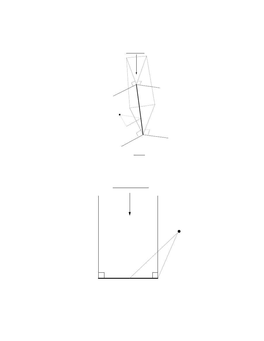
44
b
E
P
b > a
Voronoi Rgn.
a
Figure 3.9: An Overhead View for Point-Edge Applicability Criterion Proof
P
E H
E
T
E
Voronoi Region
Figure 3.10: A Side View for Point-Edge Applicability Criterion Proof

45
F
E
F
N
F
Voronoi Region
P
Figure 3.11: A Side View for Point-Face Applicability Criterion Proof
between the closest feature candidates base upon the minimum distance information
during the search.
Therefore, we can conclude that the distance decreases when a switch of
feature pairs is made as the result of Point-Face Applicability Test.
(IV) Verifying Subroutines in Edge-Face Case
With the exception of edge-edge (as mentioned earlier in the beginning of
the proof), only edge-face and face-face may have multiple pairs of closest points and
require a more complex treatments. Whereas, the closest feature verication for the
other non-degenerate cases and edge-edge solely depends on point-vertex, point-edge,
and point-face applicability tests which we have already studied. Now we will examine
each of these two cases closely.
Edge-Face
(
E, F)
The indentation corresponds to the level of nested loops in the pseudo code (Ap-
pendix B). Please cross-reference if necessary.

46
Given an edge
E and a face F, the algorithm rst checks
IF
E
AND
F
ARE
PARALLEL
, i.e. the two endpoints
H
E
and
T
E
are equi-distant from the face
F
(i.e. their signed distance is the same). The
signed
distance between
H
E
and
F can
be computed easily by
H
E
N
F
where
N
F
is
F's unit outward normal and similarly
for the signed distance between
F and H
T
.
THEN
, when the head
H
E
and tail
T
E
of the edge
E are equi-distant from the face
F, the subroutine checks
IF
E
INTERSECTS
F
'S PRISM REGION
, (i.e. the
region bounded by
F's constraint planes constructed from the edges in F's boundary).
THEN
, if
E intersects the prism region of F, the algorithm checks
IF
THE HEAD
H
E
(OR TAIL
T
E
) OF
E
LIES ABOVE THE FACE
F.
THEN
, it will check
IF THE FACE OUTWARD NOR-
MAL
N
F
IS \BOUNDED" BY THE NORMALS OF
THE EDGE'S LEFT AND RIGHT FACES
, say
N
L
and
N
R
respectively, to verify that the face
F lies inside the Voronoi
region of the edge
E, not in the Voronoi region of E's left or right
face (
F
L
or
F
R
). This is done by checking if (
N
L
~E)
N
F
> 0
and (~
E
N
R
)
N
F
> 0, where N
F
is the outward normal of the
face
F, ~E is the edge vector (as described in Sec. 2.1.2), and
N
R
,
N
L
denote the outward normal of the edge's right and left
face respectively.
THEN
, the edge
E and the face F will be returned as
the closest feature pair, since
E and F lie within the
Voronoi region of each other.
ELSE
, it returns the right or left face (
F
R
or
F
L
) of
E,
which ever is closer to
F.
ELSE
, when the head
H
E
(implies
E also) lies beneath F, then
it will invoke a subroutine
e-nd-min
which nds the closest
feature on the polyhedron
B containing F to E by enumerating
all the features on
B. Then the algorithm will return E and this
new feature
f
B
as the next candidates for the closest feature pair
verication.
ELSE
,
E does not intersect the prism dened by F's boundary edges,
then there is at least one edge of
F's boundary which is closer to E

47
than the interior of
F is to E (by the denition of Voronoi region). So,
when the test is failed, it calls a constant time routine (which takes time
proportional to the constant number of face's boundary) and returns the
edge
E and the closest edge or vertex, say f
F
, on the
F's boundary to E.
ELSE
, the algorithm checks
IF ONE END POINT LIES ABOVE THE FACE
F
AND THE OTHER LIES BENEATH
F.
THEN
, if so there is one edge on
F's boundary which is closer to E than
the interior of
F. So, the algorithm will nd the closest edge or vertex
f
B
, which has the minimum distance to
E among all edges and vertices
in
F's boundary, and return (E, f
B
) as the next candidate pair.
ELSE
, one endpoint
H
E
(or
T
E
) of
E is closer (the magnitude
j
V
E
N
F
j
instead of the signed distance is used for comparison here) to
F
than the other endpoint, the algorithm will check
IF THE CLOSER
ENDPOINT
V
E
LIES INSIDE OF
F
's PRISM REGION
(bounded
by constraint planes generated by edges in
F's boundary), Cell
F
, as in
the vertex-face case.
THEN
, if closer endpoint
V
E
lies inside of
F's prism region,
then the algorithm will next verify
IF THIS ENDPOINT
LIES ABOVE THE FACE
F (to detect a local minimum of
distance function).
THEN
, if
V
E
(the closer endpoint to
F) is above F the
algorithm next veries
IF THE CLOSEST POINT
P
F
ON
F
TO
V
E
SATISFIES
V
E
'S APPLICA-
BILITY CONSTRAINTS
.
THEN
, if so the algorithm returns
V
E
and
F
as the closest feature pair.
ELSE
some constraint plane in
V
E
's Voronoi
cell
Cell
V
E
is violated. This constraint plane is
generated by an edge, say
E
0
, in
V
E
's cobound-
ary. This edge
E
0
is closer to
F, so the algo-
rithm will return (
E
0
,
F) as the next candidate
pair.
ELSE
, if the closer endpoint
V
E
of
E lies beneath F,
then the algorithm nds the closest feature
f
B
on the
polyhedron
B to V
E
The algorithm returns (
V
E
,
f
B
) as
the next candidate feature pair.

48
ELSE
, if the closer endpoint
V
E
of
E to F lies outside of F's
prism region, then there is one edge on
F's boundary which is
closer to
E than the interior of F. So, the algorithm will nd
the closest edge or vertex
f
B
, which has the minimum distance
to
E among all edges and vertices in F's boundary, and return
(
E, f
B
) as the next candidate pair.
(V) Verifying Subroutines in Face-Face Case
Face-Face
(
F
A
,
F
B
)
The numbering system (
n) in this proof is annotated for easy reference within the
proof. The indentation corresponds to the level of nested loops in the pseudo code
(Appendix B).
(0) Given two faces,
F
A
and
F
B
, the algorithm rst checks
IF THEY ARE PAR-
ALLEL
.
(1)
THEN
, if they are parallel, it invokes a subroutines which runs in constant time
(proportional to the product of numbers of boundaries between two faces, which is a
constant after subdivision) to check
IF THE ORTHOGONAL PROJECTION
OF
F
A
ON TO THE PLANE OF
F
B
OVERLAPS
F
B
(i.e.
F
A
intersects the
prism region of
F
B
).
(2)
THEN
, if they overlapped, the algorithm next checks
IF
P
A
(implies
F
A
as well, since two faces are parallel)
LIES ABOVE
F
B
, where
P
A
is one of the points on
F
A
and its projection down to the
F
B
is in the
overlap region.
(3)
THEN
, if
P
A
(thus
F
A
) lies above
F
B
, the algorithm next
checks
IF
P
B
(THUS
F
B
) ALSO LIES ABOVE
F
A
, where
P
B
is one of the points and its projection down to the
F
B
is in
the overlap region.
(4)
THEN
, if
P
B
(thus
F
B
) is above
F
A
and vice versa,
we have a pair of closest points (
P
A
,
P
B
) satisfy the
respective applicability constraints of
F
B
and
F
A
. So,
P
A
and
P
B
are the closest points on
A and B; and the

49
features containing them,
F
A
and
F
B
, will be returned
as the closest features.
(5)
ELSE
, if
P
B
(thus
F
B
) lies beneath
F
A
, then the
algorithm nds the closest feature
f
A
on polyhedron
A
containing
F
A
to
F
B
by enumerating all features of
A to
search for the feature which has minimum distance to
F
B
. So, the new pair of features (
f
A
,
F
B
) is guaranteed
to be closer than (
F
A
,
F
B
).
(6)
ELSE
, if
P
A
(thus
F
A
) lies beneath
F
B
, the algorithm nds
the closest feature
f
B
on polyhedron
B containing F
B
to
F
A
and
returns (
F
A
,
f
B
) as the next candidate feature pair. This pair
of new features has to be closer than
F
A
to
F
B
since
f
B
has the
shortest distance among all features on
B to F
A
.
(7)
ELSE
, if
F
A
and
F
B
are parallel but the projection of
F
A
does not
overlap
F
B
, a subroutine enumerates all possible combination of edge-
pairs (one from the boundary of each face respectively) and computes the
distance between each edge-pair to nd a pair of closest edges which has
the minimum distance among all. This new pair of edges (
E
A
,
E
B
) is
guaranteed to be closer than the two faces, since two faces
F
A
and
F
B
do
not contain their boundaries.
(8)
ELSE
, if
F
A
and
F
B
are not parallel, this implies there is at least one vertex or
edge on
F
A
closer to
F
B
than
F
A
to
F
B
or
vice versa. So, the algorithm rst nds
the closest vertex or edge on
F
A
to the plane containing
F
B
,
B
.
(9)
VERTEX:
if there is only a single closest vertex
V
A
to the plane
containing
F
B
,
V
A
is closer to
F
B
than
F
A
is to
F
B
since two faces are
not parallel and their boundaries must be closer to each other than their
interior. Next, the algorithm checks if
V
A
lies within the Voronoi region
of
F
B
.
(10)
THEN
, if so
V
A
and
F
B
will be returned as the next can-
didate pair.
(11)
ELSE
, the algorithm nds the closest vertex (or edge) on
F
B
to
A
, and proceeds as before.
(12)
VERTEX:
if there is only a single vertex
V
B
clos-
est to the plane
A
containing
F
A
, the algorithm checks
if
V
B
lies inside of
F
A
's Voronoi region bounded by the
constraint planes generated by the edges in
F
A
's bound-
ary and above
F
A
.

50
(13)
THEN
, if
V
B
lies inside of
F
A
's Voronoi
region, then
F
A
and
V
B
will naturally be the
next candidate pair. This new pair of features
is closer than the previous pair as already ana-
lyzed in (10).
(14)
ELSE
, the algorithm performs a search of
all edge pairs from the boundary of
F
A
and
F
B
and returns the closest pair (
E
A
,
E
B
) as the
next candidate feature pair.
(15)
EDGE:
, similarly if the closest feature on
F
B
to
A
is an edge
E
B
, the algorithm once again checks if
E
B
cuts
F
A
's prism to determine whether
F
A
and
E
B
are the next candidate features.
(16)
THEN
, the algorithm checks
IF THE
END POINT OF
E
B
LIES ABOVE
F
A
.
(17)
THEN
, the new pair of candidate
features is
F
A
and
E
B
since
E
B
lies within
F
A
's Voronoi region.
(18)
ELSE
, the algorithm searches for the
closest feature
f
A
which has the minimum
distance among all other features on
A to
E
B
and returns (
f
A
,
E
B
) as the next pair
of candidate features.
(14)
ELSE
, if not, then this implies that nei-
ther face contains the closest points since nei-
ther
F
A
nor
F
B
's Voronoi regions contain a clos-
est point from the other's boundary. So, the
algorithm will enumerate all the edge-pairs in
the boundaries of
F
A
and
F
B
to nd the pair of
edges which is closest in distance. This new
pair of edges (
E
A
,
E
B
) is guaranteed to be
closer than the two faces.
(19)
EDGE:
if there are two closest vertices on
F
A
to
B
, then the edge
E
A
containing the two vertices is closer to
B
than
F
A
is. Next, the
algorithm checks
IF
E
A
INTERSECTS THE PRISM REGION OF
F
B
, as in the edge-face case.
(20)
THEN
, the algorithm checks
IF THE END POINT
OF
E
A
LIES ABOVE
F
B
.
(21)
THEN
, if so the edge
E
A
and
F
B
will be returned
as the next candidate pair.

51
(22)
ELSE
, the algorithm searches for the closest fea-
ture
f
B
which has the minimum distance among all
other features on
B to E
A
and returns (
E
A
,
f
B
) as the
next pair of candidate features.
(23)
ELSE
, if this is not the case, then the algorithm nds the
closest vertex (or edge) on
F
B
to the plane containing
F
A
, say
A
and proceeds as before, from block (11) to block (18).
In either degenerate case (edge-face or face-face), a pair of features closer
in distance is always provided when a switch of feature pairs is made. All the veri-
fying subroutines run in
constant
time (proportional to the number of boundary or
coboundary of features
or
the product of numbers of boundaries between two fea-
tures), except where an edge lies beneath a face or when a face lies beneath a face.
In such local cases, a linear-time routine is invoked.
To sum up, all the applicability tests and closest feature-pair verifying sub-
routines generate a pair of new features closer in distance than the previous pair when
a switch of feature-pairs is made.
Corollary
The algorithm takes
O(n
3
) time to nd the closest feature pair, since
each pair of features is visited at most once, and each step takes at most linear time.
O(n
3
) is a rather loose upper bound. We can nd a tighter bound on the
running time if we study the local minimum case in greater details. As a result of
a new analysis, we claim in Lemma 2 that the algorithm should converge in
O(n
2
)
time. The proof is stated below.
Lemma 2
The algorithm will converge in
O(n
2
) time.
Proof:
Except for the case of a local minimum which corresponds to the situation
where one feature lies under the plane containing the other face, all the applicability
tests and subroutines run in constant time. Thus the overall running time is
O(n
2
)
in this case, since the algorithm can only exhaustively visit
O(n
2
) pairs of features

52
and no looping can possibly exist if it doesn't encounter local minima (by Lemma 1).
As mentioned earlier, when a local minimum is encountered, a linear-time routine is
invoked. But it is not necessary to call this linear-time routine more than 2
n times
to nd the closest feature-pair. The reasons are the following:
We claim that we will not revisit the same feature twice in a linear time
check. We will prove by contradiction. Assume that the linear time routine is called
to nd a closest feature in
B to f
A
. The routine will never again be called with (
f
A
,
B) as argument. Suppose it was, i.e. suppose that f
B
was the result of the call to
the linear time routine with input (
f
A
;B) and after several iterations from (f
A
,
f
B
)
!
:::
!
(
f
0
A
,
f
0
B
) we come to a feature pair (
f
A
,
f
0
B
) and that the linear routine is
invoked to nd the closest feature on
B to f
A
. Once again,
f
B
must be returned as
the closest feature to
f
A
. But, this violates Lemma 1 since the distance must strictly
decrease when changes of features are made, which is not true of the regular sequence
(
f
A
;f
B
)
!
:::
!
(
f
A
;f
0
B
)
!
:::
!
(
f
A
;f
B
).
Similarly, the routine will not be called more than once with (
f
B
, A) as
arguments. Thus, the linear-time routine can be called at most 2
n times, where n is
the total number of features of object
B (or A).
Therefore, the closest-feature algorithm will converge in
O(n
2
) time, even in
the worst case where local minima are encountered.
3.5 Numerical Experiments
The algorithm for convex polyhedral objects described in this chapter has
been implemented in both Sun Common Lisp and ANSI C for general convex objects.
(The extension of this algorithm to non-convex objects is presented in the next chap-
ter.) The input data are arbitrary pairs of features from two given polyhedral objects
in three dimensional space. The routine outputs a pair of the closest features (and
a pair of nearest points) for these two objects and the Euclidean distance between
them.
Numerous examplesin three dimensionalspace have been studied and tested.
Our implementation in ANSI C gives us an expected constant time performance of
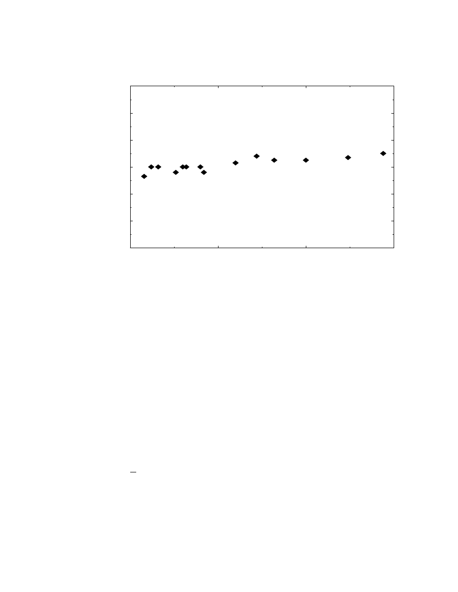
53
0.0
100.0
200.0
300.0
total number of vertices
0.0
20.0
40.0
60.0
80.0
100.0
120.0
computation time in microseconds
Figure 3.12: Computation time vs. total no. of vertices
50-70 usec per object pair of arbitrary complexity on SGI Indigo2 XZ (200-300 usec
per object pair on a 12.5 Mips 1.4 Mega ops Sun4 Sparc Station) for relative small
rotational displacement. Fig.3.12 shows the expected constant time performance for
polygonized spherical and cylindrical objects of various resolutions. Each data point
is taken as the average value of 1000 trials with the relative rotation of 1 degree per
step. (The closest features rarely change if two objects are translated along the line
connecting the closest feature pair.)
We would like to mention that the accumulated runtime for 1000 trials
shows slightly increasing trend for total vertices over 1000, this is due to the fact
that the number of feature pair changes for the same amount of rotation increases
if the resolution of objects increases. For spherical and most objects, the runtime is
roughly
O(
p
n) where n is number of vertices for each object with a extremely small
constant. For the cylindrical objects where the total number of facets to approximate
the quadratic surface is linear with the number of vertices, the total accumulated
runtime is expectedly sub-linear with the total number of vertices.

54
For two convex hulls of teapots (each has 1047 vertices, 3135 edges, and 2090
faces), the algorithm takes roughly 50, 61, 100, 150 usec for 1, 5, 10, 20 degrees of
relative rotation and displacements. Note that when the relative movement between
2 objects becomes large, the runtime seems to increase as well, this is due to the fact
that the geometric coherence doesn't hold as well in the abrupt motions. Nevertheless,
the algorithm continues to perform well compared to other algorithms.
The examples we used in our simulation include a wide variety of polytopes:
cubes, rectangular boxes, cylinders, cones, frustrums, and a Puma link of dierent
sizes as shown in Fig.3.13. In particular, the number of facets or the resolution for
cylinders, cones and frustrums have been varied from 12, 20, 24, 48, up to 120 in order
to generate a richer set of polytopes for testing purpose. Due to the programming
language's nature, Lisp code usually gives a longer run time (roughly 10 times slower
than the implementation written in ANSI C).
To give readers a feeling of speed dierence the expected run time obtained
from our Lisp code is 3.5 msec which is roughly 10 times slower than our C imple-
mentation (from the same Sun4 SPARC station described above), independent of
object complexity. The experiment results obtained from our Lisp code are briey
summarized in Table 1. M1 and M2 stand for the number of vertices for each object
respectively; and N stands for the total number of vertices between the two objects.
The average CPU time is taken over 50 trials of experimental runs. (Each trial picks
all 18 arbitrary permuted combination of feature pairs to initialize the computation
and calculates the average run time based upon these 18 runs.) With initialization to
the previous closest feature, the routine can almost always keep track of the closest
features of two given polytopes in expected constant time (about 3 to 4 msec).
Without initialization (i.e. no previous closest feature pair is given), the
algorithm runs in average time not worse than linear in the total number of vertices.
This is what we would expect, since it seems unlikely that the algorithm would need to
visit a given feature more than once. In practice, we believe our algorithm compares
very favorably with other algorithms designed for distance computations or collision
detection. Since the nature of problem is not the same, we cannot provide exact
comparisons to some of the previous algorithms. But, we can briey comment on the
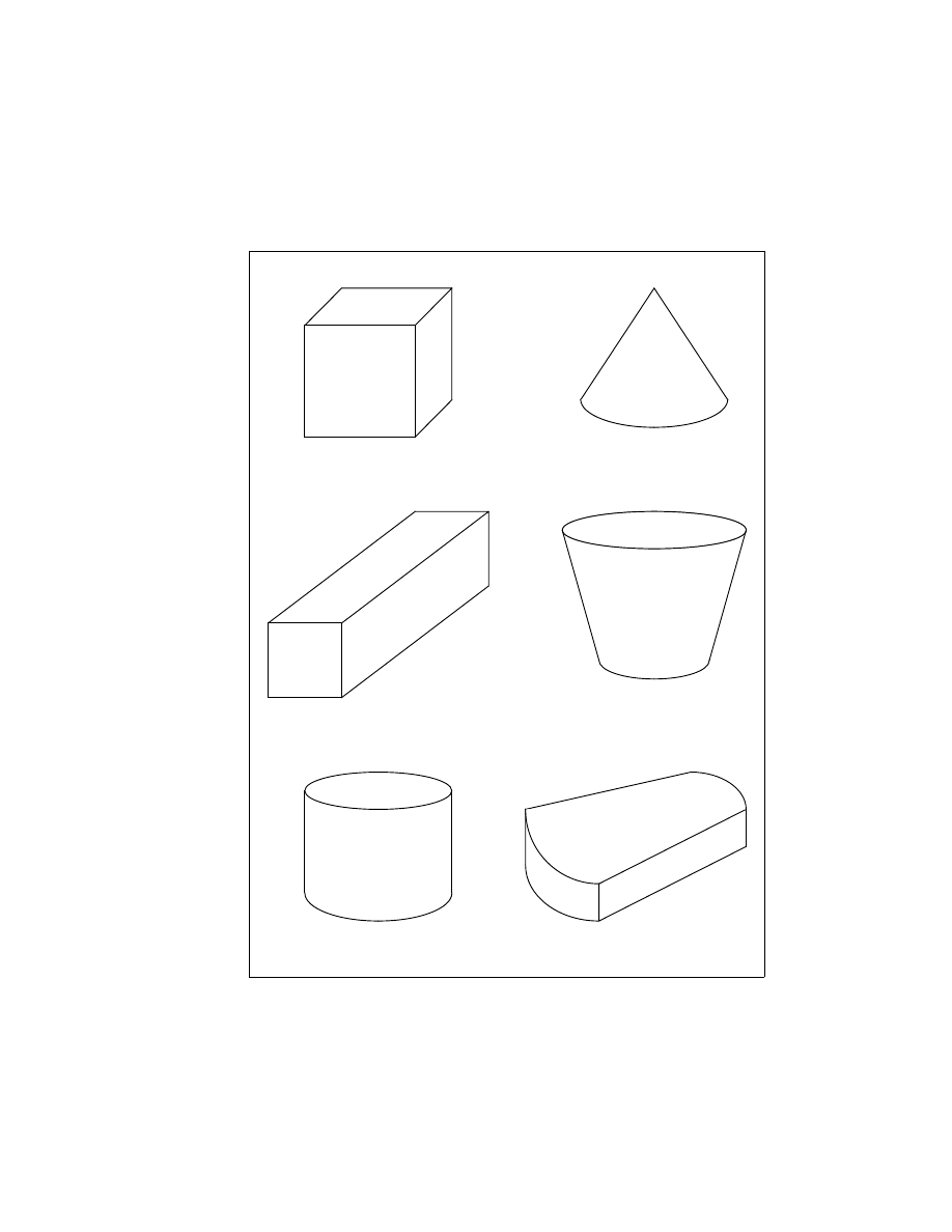
55
(a)
(b)
(c)
(d)
(e)
(f)
Figure 3.13: Polytopes Used in Example Computations

56
Objects M1 + M2 = N w/o Init w/ Init
(a),(b)
8 + 8 = 16
21
3.2
(a),(f)
8 + 16 = 24
23
3.3
(a),(c)
8 + 24 = 32
26
3.5
(d),(e)
48 + 21 = 69
41
3.5
(c),(c) 96 + 48 = 144
67
3.0
Table 3.1: Average CPU Time in Milliseconds
number of operations involved in a typical calculation. For an average computation
to track or update a pair of closest features, each run takes roughly 50-70 usec on a
SGI Indigo2 XZ or 92-131 arithmetic operations (roughly 12-51 operations to nd the
nearest points, 2 x 16 operations on 2 point transformations, 2 x 4 x 6 operations for
two applicability tests and each involves 4 inner product calculations) independent
of the machines. By comparing the number of arithmetic operations in the previous
implementedalgorithms, we believethat our implementationgives better performance
and probably is the fastest implementedcollision detection algorithm. (Please see [65],
[13], [17], [40], [39], [38], [72], and [90].)
This is especially true in a dynamic environment where the trajectories are
not known (nor are they in closed form even between impacts, but are given by ellip-
tic integrals). The
expected constant time
performance comes from the fact that
each
update
of the closest feature pair involves only the constant number of neighboring
features (after the initialization and preprocessing procedures). The speed of algo-
rithm is an attribute from the
incremental
nature of our approach and the geometric
coherence between successive, discrete movements.
3.6 Dynamic Collision Detection for Convex Poly-
hedra
The distance computation algorithm can be easily used for detecting colli-
sion while the objects are moving. This is done by iteratively checking the distance

57
between any pair of moving objects. If the distance is less than or equal to zero (plus
- a small safety margin dened by the user), then a collision is declared. We can set
the step size of the algorithm once we obtain the initial position, distance, velocity
and acceleration among all object pairs. We also use a simple queuing scheme to
reduce the frequency of collision checks by relying on the fact that only the object
pairs which have a small (Chapter 5).
Furthermore, we will not need to transform all the Voronoi regions and all
features of polyhedra but only the closest points and the new candidate features (if
necessary), since local applicability constraints are all we need for tracking a closest
pair of closest features. The transformation is done by taking the relative transfor-
mation between two objects. For example, given two objects moving in space, their
motions with respect to the origin of the world frame can be characterized by the
transformation matrices
T
A
and
T
B
respectively. Then, their relative motion can be
represented by the homogeneous relative transformation
T
AB
=
T
,1
B
T
A
.

58
Chapter 4
Extension to Non-Convex Objects
and Curved Objects
Most of objects in the real world are not simple, convex polyhedral objects.
Curved corners and composite objects are what we see mostly in the man-made envi-
ronment. However, we can use the union of convex polyhedra to model a non-convex
object and reasonably rened polyhedral approximation for curved boundaries as well.
In this chapter, we will discuss how we extend the collision detection algorithm (de-
scribed in Chapter 3) from convex objects to non-convex objects. Then, the extension
to the curved objects will be described later in the chapter as well.
4.1 Collision Detection for Non-convex Objects
4.1.1 Sub-Part Hierarchical Tree Representation
Nonconvex objects can be either composite solid objects or they can be
articulated bodies. We assume that each nonconvex object is given as a union of
convex polyhedra
or
is composed of several nonconvex subparts, each of these can be
further represented as a union of convex polyhedra or a union of non-convex objects.
We use a sub-part hierarchy tree to represent each nonconvex object. At each node of
the tree, we store either a convex sub-part (at a leave) or the union of several convex

59
Figure 4.1: An example of sub-part hierarchy tree

60
subparts.
Depending on the applications, we rst construct the convex hull of a rigid
non-convex object or dynamic bounding box for articulated bodies at each node and
work up the tree as part of preprocessing computation. We also include the convex
hull or dynamic bounding box of the union of sub-parts in the data structure. The
convex hull (or the bounding box) of each node is the convex hull (or bounding box)
of the union of its children. For instance, the root of the sub-part hierarchy tree for
a composite solid non-convex object is the nonconvex object with its convex hull in
its data structure; each convex sub-part is stored at a leave. The root of the sub-part
hierarchical tree for a Puma arm is the bounding box of the entire arm which consists
of 6 links; and each leave stores a convex link.
For example, in Fig. 4.1, the root of this tree is the aircraft and the convex
hull of the aircraft (outlined by the wire frames). The nodes on the rst level of the
tree store the subparts and the union of the subparts of the aircraft, i.e. the left and
right wings (both convex), the convex body of airplane, and the union of the tail
pieces. Please note that at the node where the union of the tail pieces are stored, a
convex hull of union of these tail pieces is also stored there as well. This node, which
stores the union of all tail pieces, further branches out to 3 leaves, each of which
stores a convex tail piece.
For a robot manipulator like a Puma arm, each link can be treated as a
convex subpart in a leave node. The root of this tree can be a simple bounding box of
the entire Puma arm whose conguration may be changing throughout the duration
of its task. (Therefore, the bounding box may be changing as well. Of course, the
eciency of our distance computation algorithm in Chapter 3 is lost when applied
to a changing volume, since the Voronoi regions will be changing as the volume of
the object changes and the preprocessing computation is not utilized to its maximum
extend. However, in Chapter 5 we will present another simple yet ecient approach
to deal with such a situation.)
In addition, not only can we apply the hierarchical subpart tree representa-
tion to polyhedral models, we can also use it for non-convex
curved
objects as well.
Depending on the representation of the curved objects (parametric, algebraic, Bezier,

61
or B-spline patches), each node of the tree will store a portion (such as a patch) of
the curved surfaces and the root of the tree is the entire curved object and the convex
hull of its polyhedral approximation. For more treatments on the non-convex curved
objects, please refer to Sec. 4.3.3.
4.1.2 Detection for Non-Convex Polyhedra
Given the subpart tree representation, we examine the possible interference
by a recursive algorithm at each time step. The algorithm will rst check for collision
between two parent convex hulls. Of course, if there is no interference between two
parents, there is no collision and the algorithm updates the closest-feature pair and the
distance between them. If there is a collision, then it will expand their children. All
children of one parent node are checked against all children of the other parent node.
If there is also a collision between the children, then the algorithm will recursively call
upon itself to check for possible impacts among the children's children, and so on. In
this recursive manner, the algorithm will only signal a collision if there is actually an
impact between the sub-parts of two objects; otherwise, there is no collision between
the two objects.
For instance, assume for simplicitythat one nonconvex object is composed of
m convex polyhedra and the other is composed of n convex polyhedra, the algorithm
will rst check for collision between the two convex hulls of these two objects. If there
is a collision,
mn convex polyhedra-pairs will be tested for possible contacts. If there
is a collision between any one of these
mn pairs of convex polyhedra, then the two
objects interpenetrate; otherwise, the two objects have not yet intersected. Fig. 4.2
shows how this algorithm works on two simplied aircraft models.
In Fig. 4.2, we rst apply the algorithm described in Chapter 3 to the convex
hulls of the two aircrafts. If they do not intersect, then the algorithm terminates and
reports no collision. In the next step, the algorithm continues to track the motion of
the two planes and nds their convex hulls overlap. Then, the algorithm goes down
the tree to the next level of tree nodes and check whether there is a collision among
the subparts (the wings, the bodies, and the union of subparts, i.e. the union of tail

62
pieces). If not, the algorithm will not report a collision. Otherwise, when there is an
actual penetration of subparts (such as two wings interpenetrating each other), then
a collision is reported.
We would like to clarify one fact that we never need to construct the Voronoi
regions of the non-convex objects, since it is absolutely unnecessary given the subpart
hierarchical tree. Instead, at the preprocessing step we only construct the Voronoi
regions for each convex piece at each node of the subpart hierarchical tree. When we
perform the collision checks, we only keep track of the closest feature pairs for the
convex hulls of parent nodes, unless a collision has taken place between the convex
hulls of two non-convex objects or the bounding boxes of articulated bodies. Under
such a situation, we have to track the closest pair of features for not only the convex
hulls or bounding boxes at the parent nodes, but also among all possible subpart
pairs at the children nodes as well. This can lead to
O(n
2
) of comparisons, if each
object is consisted of
n subparts and the trees only have two levels of leave nodes.
However, we can achieve a better performance if we have a good hierarchy of
the model. For complex objects, using a deep hierarchical tree with lower branching
factor will keep down the number of nodes which need to be expanded. This approach
guarantees that we nd the earliest collision between two non-convex objects while
reducing computation costs. For example, given 2
n subparts, we can further group
them into two subassemblies and each has
n subparts. Each subassembly is further
divided into several smaller groups. This process generates a deep hierarchical tree
with lower branching factor, thus reduces the number of expansions needed whenever
the convex hulls (or bounding boxes) at the top-level parent nodes collide.
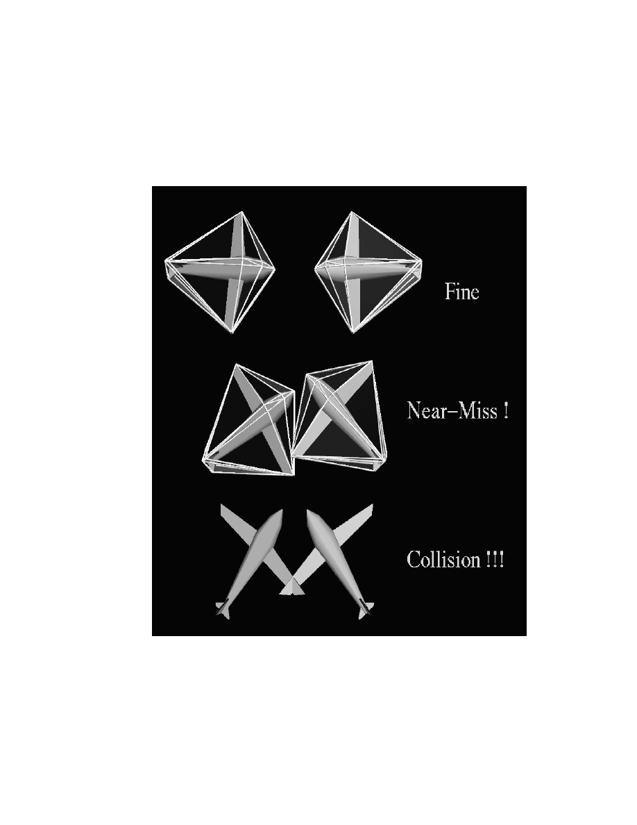
63
Figure 4.2: An example for non-convex objects

64
4.2 Collision Detection for Curved Objects
In this section
1
, we analyze the problemof collision detection between curved
objects represented as spline models or piecewise algebraic surfaces. Dierent types of
surface representations have been desribed in Chapter 2, please refer to it if necessary.
We show that these problems reduce to nding solutions of a system of algebraic
equations. In particular, we present algebraic formulations corresponding to closest
points determination and geometric contacts.
4.2.1 Collision Detection and Surface Intersection
In geometric and solid modeling, the problem of computing the intersection
of surfaces represented as spline surfaces or algebraic surfaces has received a great
deal of attention [46]. Given two surfaces, the problem corresponds to computing all
components of the intersection curve robustly and accurately. However, for collision
detection we are actually dealing with a restricted version of this problem. That is,
given two surfaces we want to know whether they intersect.
In general, given two spline surfaces, there is
no
good and quick solution
to the problem of whether they intersect or have a common geometric contact. The
simplest solution is based on checking the control polytopes (a convex bounding box)
for collision and using subdivision. However, we have highlighted the problems with
this approach (in Chapter 1) in terms of performance when the two objects are close
to touching. Our approach is based on formulating the problem in terms of solving
systems of algebraic equations and using global methods for solving these equations,
and local methods to update the solutions.
4.2.2 Closest Features
Given the homogeneous representation of two parametric surfaces,
F
(
s;t) =
(
X(s;t), Y (s;t), Z(s;t), W(s;t)) and
G
(
u;v) = (X(u;v), Y (u;v);Z(u;v), W(u;v));
1
This is the result of joint work with Prof. Dinesh Manocha at the University of North Carolina,
Chapel Hill

65
the closest
features
between two polyhedra correspond to the closest point sets on the
surface. The closest points are characterized by the property that the correspond-
ing surface normals are collinear. This can be expressed in terms of the following
variables. Let
F
11
(
s;t;u;v;
1
) = (
F
(
s;t)
,
G
(
u;v))
F
12
(
s;t;u;v;
1
) =
1
(
G
u
(
u;v)
G
v
(
u;v))
F
21
(
s;t;u;v;
2
) = (
F
s
(
s;t)
F
t
(
s;t))
F
22
(
s;t;u;v;
2
) =
2
(
G
u
(
u;v)
G
v
(
u;v));
where
F
s
;
F
t
;
G
u
;
G
v
correspond to the partial derivatives. The closest points between
the two surfaces satisfy the following equations:
F
1
(
s;t;u;v;
1
) =
F
11
(
s;t;u;v;
1
)
,
F
12
(
s;t;u;v;
1
) =
0
B
B
B
B
@
0
0
0
1
C
C
C
C
A
:
(4.1)
F
2
(
s;t;u;v;
2
) =
F
21
(
s;t;u;v;
2
)
,
F
22
(
s;t;u;v;
2
) =
0
B
B
B
B
@
0
0
0
1
C
C
C
C
A
:
This results in 6 equations in 6 unknowns. These constraints between the closest
features can also be expressed as:
H
1
(
s;t;u;v) = (
F
(
s;t)
,
G
(
u;v))
G
u
(
u;v) = 0
H
2
(
s;t;u;v) = (
F
(
s;t)
,
G
(
u;v))
G
v
(
u;v) = 0
(4.2)
H
3
(
s;t;u;v) = (
F
(
s;t)
,
G
(
u;v))
F
s
(
s;t) = 0
H
4
(
s;t;u;v) = (
F
(
s;t)
,
G
(
u;v))
F
t
(
s;t) = 0;
where
corresponds to the dot product. This results in four equations in four un-
knowns.
Let us analyze the algebraic complexityof these two system of equations cor-
responding to closest features. Lets consider the rst system corresponding to (4.1).
In particular, given 2 rational parametric surfaces
F
(
s;t) and
G
(
u;v), both of their

66
numerators and denominators are polynomials of degree
n, the degrees of numerators
and denominators of the partials are 2
n
,
1 and 2
n respectively in the given vari-
ables (due to quotient rule). The numerator and denominator of
F
11
(
s;t;u;v;
1
)
have degree 2
n and 2n due to subtraction of two rational polynomials. As for
F
12
(
s;t;u;v;
1
), taking the cross product doubles the degrees for both the numer-
ator and denominator; therefore, the degrees for the numerator and denominator of
F
12
(
s;t;u;v;
1
) are 4
n
,
2 and 4
n respectively. To eliminate
1
from
F
1
(
s;t;u;v;
1
),
we get
F
11
(
X(s;t;u;v;
1
))
F
12
(
X(s;t;u;v;
1
)) =
F
11
(
Y (s;t;u;v;
1
))
F
12
(
Y (s;t;u;v;
1
)) =
F
11
(
Z(s;t;u;v;
1
))
F
12
(
Z(s;t;u;v;
1
))
(4
:3)
After cross multiplication to clear out the denominators we get two
polynomails
of
degree 12
n
,
2 each. Once again, by the same reasoning as stated above, both the
numerators and denominators of
F
21
(
s;t;u;v;
2
) and
F
22
(
s;t;u;v;
2
) have degrees
of 4
n
,
2 and 4
n. By similar method mentioned above, we can eliminate
2
from
F
2
(
s;t;u;v;
2
). We get two polynomial equations of degree 16
n
,
4 each after cross
multiplication. As a result the system has a Bezout bound of (12
n
,
2)
2
(16
n
,
4)
2
.
Each equation in the second system of equations has degree 4
n
,
1 (obtained
after computing the partials and addition of two rational polynomials) and therefore
the overall algebraic complexitycorresponding to the Bezout bound is (4
n
,
1)
4
. Since
the later system results in a lower degree bound, in the rest of the analysis we will
use this system. However, we are only interested in the solutions in the domain of
interest (since each surface is dened on a subset of the real plane).
Bara has used a formulation similar to (4.1)to keep track of closest points
between closed convex surfaces [3] based on local optimization routines. The main
problem is nding a solution to these equations for the initial conguration. In
general, these equations can have more than one solution in the associated domain, i.e.
the real plane, (even though there is only one closest point pair) and the optimization
routine may not converge to the right solution. A simple example is the formulation
for the problem of collision detection between two spheres. There is only one pair of
closest points, however equations (4.1) or (4.2) have four pairs of real solutions.
Given two algebraic surfaces,
f(x;y;z) = 0 and g(x;y;z) = 0, the problem

67
( a )
Tangent Plane
Contact Point
Intersection
is a boundary point
( b )
Figure 4.3: Tangential intersection and boundary intersection between two Bezier
surfaces
of closest point determination can be reduced to nding roots of the following system
of 8 algebraic equations:
f(x
1
;y
1
;z
1
) = 0
g(x
2
;y
2
;z
2
) = 0
(4.4)
0
B
B
B
B
@
f
x
(
x
1
;y
1
;z
1
)
f
y
(
x
1
;y
1
;z
1
)
f
z
(
x
1
;y
1
;z
1
)
1
C
C
C
C
A
=
1
0
B
B
B
B
@
g
x
(
x
2
;y
2
;z
2
)
g
y
(
x
2
;y
2
;z
2
)
g
z
(
x
2
;y
2
;z
2
)
1
C
C
C
C
A
0
B
B
B
B
@
x
1
y
1
z
1
1
C
C
C
C
A
,
0
B
B
B
B
@
x
2
y
2
z
2
1
C
C
C
C
A
=
2
0
B
B
B
B
@
g
x
(
x
2
;y
2
;z
2
)
g
y
(
x
2
;y
2
;z
2
)
g
z
(
x
2
;y
2
;z
2
)
1
C
C
C
C
A
Given two algebraic surfaces of degree
n, we can eliminate
1
by setting
f
x
(
x
1
;y
1
;z
1)
g
x
(
x
2
;y
2
;z
2
)
=
f
y
(
x
1
;y
1
;z
1)
g
y
(
x
2
;y
2
;z
2)
. After cross multiplication, we have a polynomial equation
of 2n-2, since each partial has degree of
n
,
1 and the multiplication results in

68
the degree sum of 2
n
,
2. To eliminate
2
, we set
x
1
,
x
2
g
x
(
x
2
;y
2
;z
2
)
=
y
1
,
y
2
g
y
(
x
2
;y
2
;z
2
)
and the
degree of the resulting polynomial equation is n. We have six quations after elim-
inating
1
and
2
: two of degrees (2
n
,
2) and four of degress
n respectively (2
from eliminating
2
and 2 from
f(x
1
;y
1
;z
1
) and
g(x
2
;y
2
;z
2
)). Therefore, the Bezout
bound of the resulting system can be as high as
N = (2n
,
2)
2
n
4
. In general, if
the system of equations is sparse, we can get a tight bound with Bernstein bound
[8]. The Bernstein bound for Eqn. 4.4 is
n
2
(
n
2
+ 3)(
n
,
1)
2
. Canny and Emiris
calculate the Bernstein bounds eciently by using sparse mixed resultant formula-
tion [16]. For example, the Bernstein bounds
2
for the case of
n = 2;3;4;5;6;7;8;9
are 28
;432;2736;11200;35100;91728;210112;435456, while the Bezout bounds are
64
;1296;9216;40000;129600;345744;
respectively. Even for small values of
n, N
can be large and therefore, the algebraic complexity of computing the closest points
can be fairly high. In our applications we are only interested in the real solutions to
these equations in the corresponding domain of interest. The actual number of real
solutions may change as the two objects undergo motion and some congurations can
result in innite solutions (e.g. when a closest pair corresponds to a curve on each
surface, as shown for two cylinders in Fig. 4.4. ). As a result, it is fairly non-trivial to
keep track of all the closest points between objects and updating them as the objects
undergo motion.
4.2.3 Contact Formulation
The problem of collision detection corresponds to determining whether there
is any contact between the two objects. In particular, it is assumed that in the
beginning the objects are not overlapping. As they undergo motion, we are interested
in knowing whether there is any contact between the objects. There are two types
of contacts. They are tangential contact and boundary contact. In this section, we
formulate both of these problems in terms of a system of algebraic equations. In the
next section, we describe how the algorithm tests for these conditions as the object
2
These gures are calculated by John Canny and Ioannis Emiris using their code based on the
sparse mixed resultant formulation.

69
undergoes rigid motion.
Tangential Intersection :
This corresponds to a tangential intersection between
the two surfaces at a geometriccontact point, as in Fig.4.3(a). The contact point
lies in the interior of each surface (as opposed to being on the boundary curve)
and the normal vectors at that point are collinear. These constraints can be
formulated as:
F
(
s;t) =
G
(
u;v)
(4.5)
(
F
s
(
s;t)
F
t
(
s;t))
G
u
(
u;v) = 0
(
F
s
(
s;t)
F
t
(
s;t))
G
v
(
u;v) = 0
The rst vector equation corresponds to a contact between the two surfaces and
the last two equations represent the fact that their normals are collinear. They
are expressed as scalar triple product of the vector The last vector equation
represented in terms of cross product corresponds to three scalar equations.
We obtain 5 equations in 4 unknowns. This is an overconstrained system and
has a solution only when the two surfaces are touching each other tangentially.
However, we solve the problem by computing all the solutions to the rst four
equations using global methods and substitute them into the fth equation. If
the given equations have a common solution, than one of the solution of the
rst four equation will satisfy the fth equation as well. For the rst three
equations, after cross multiplication we get 3 polynomial equations of degree
2
n each. The dot product results in the addition of degrees of the numerator
polynomials. Therefore, we get a polynomial equation of degree 6
n
,
3 from
the fourth equation. Therefore, the Bezout bound of the system corresponding
to the rst four equations is bounded by
N = (2n)
3
(6
n
,
3), where
n is the
parametric degree of each surface. Similarly for two algebraic surfaces, the
problem of tangential intersection can be formulated as:
f(x;y;z) = 0
g(x;y;z) = 0
(4.6)

70
0
B
B
B
B
@
f
x
(
x;y;z)
f
y
(
x;y;z)
f
z
(
x;y;z)
1
C
C
C
C
A
=
0
B
B
B
B
@
g
x
(
x;y;z)
g
y
(
x;y;z)
g
z
(
x;y;z)
1
C
C
C
C
A
In this case, we obtain 4 equations in 3 unknowns (after eliminating
) and
these equations correspond to an overconstrained system as well. These over-
constrained system is solved in a manner similar to that of parametric surfaces.
The rst two equations are of degrees
n. To eliminate from the third equa-
tion, we get a polynomial equation of degree 2(n-1) due to cross multiplication
and taking partial with respect to
x;y;z. The Bezout bound for the rst three
equations is
N = n
2
(2
n
,
2).
Boundary Intersection :
Such intersections lie on the boundary curve of one
of the two surfaces. Say we are given a Bezier surface, dened over the domain,
(
s;t)
2
[0
;1]
[0
;1], we obtain the boundary curves by substituting s or t to be
0 or 1. The resulting problem reduces to solving the equations:
F
(
s;1) =
G
(
u;v)
(4
:7)
Other possible boundary intersections can be computed in a similar manner.
The intersection points can be easily computed using global methods. An ex-
ample has been shown in Figure 4.3(b)
Two objects collide if one of these sets of equations, (4.5) or (4.7) for para-
metric surfaces and (4.6) for algebraic surfaces, have a common solution in their
domain.
In a few degenerate cases, it is possible that the system of equations (4.5)
and (4.7) have an innite number of solutions. One such example is shown for two
cylinders in Fig.4.4. In this case the geometric contact corresponds to a curve on each
surface, as opposed to a point. These cases can be detected using resultant methods
as well [55].

71
( a )
( b )
Closest
Points
Point Sets
Closest
Figure 4.4: Closest features between two dierent orientations of a cylinder
4.3 Coherence for Collision Detection between
Curved Objects
In most dynamic environments, the closest features or points between two
moving objects change infrequently between two time frames. We have used this
coherence property in designing the expected constant time algorithm for collision
detection among convex polytopes and applied to non-convex polytopes as well. In
this section we utilize this coherence property along with the algebraic formulations
presented in the previous section for curved models.
4.3.1 Approximating Curved Objects by Polyhedral Mod-
els
We approximate each physical object with curved boundary by a polyhedra
(or polygonal mesh). Such approximations are used by rendering algorithms utiliz-

72
ing polygon rendering capabilities available on current hardware. These polyhedral
models are used for collision detection, based on the almost constant time algorithm
utilizing local features. Eventually a geometric contact is determined by solving the
equations highlighted in the previous section. We use an
-polytope
approximation
for a curved surface. It is dened as:
Denition:
Let
S be a surface and P is -polytope approximation, if for all points,
p
on the boundary of polytope
P, there is a point
s
on
S such that
k
s
,
p
k
.
Similarly for each point
s
on
S, there is a point
p
on the boundary of
P such that
k
p
,
s
k
.
An
-polytope approximation is obtained using either a simple mesh gener-
ation algorithm or an adaptive subdivision of the surfaces. Given a user dened
,
algorithms for generating such meshes are highlighted for parametric B-spline surfaces
in [36] and for algebraic surfaces in [44]. In our implementation we used an inscribed
polygonal approximation to the surface boundary.
We use the
-polytope approximations for convex surfaces only. In such
cases the resulting polytope is convex as well. Often a curved model can be repre-
sented as a union of convex objects. Such models are represented hierarchically, as
described in Section 4.1.1. Each polytope at a leaf node corresponds to an
-polytope
approximation.
4.3.2 Convex Curved Surfaces
In this section we present an algorithm for two convex spline surfaces. The
input to the algorithm are two convex B-spline surfaces (say
S
A
and
S
B
) and their
associated control polytopes. It is assumed that the surfaces have at least rst order
continuity. We compute an
-polytope approximation for each spline surface. Let P
A
and
P
b
be
A
-polytope and
B
-polytope approximations of
S
A
and
S
B
, respectively.
If the objects do not collide, there may be no need to nd the exact closest
points between them but a rough estimate of location to preserve the property of
geometric coherence. In this case, we keep track of the closest points between
P
A
and
P
B
. Based on those closest points, we have a good bound on the actual distance

73
between the two surfaces. At any instance let
d
p
be the minimum distance between
P
A
and
P
B
(computed using the polyhedral collision detection algorithm). Let
d
s
be
the minimumdistance between the two surfaces. It follows from the
-approximation:
d
p
,
A
,
B
d
s
d
p
:
(4
:8)
The algorithm proceeds by keeping track of the closest points between
P
A
and
P
B
and
updating the bounds on
d
s
based on
d
p
. Whenever
d
p
A
+
B
, we use Gauss Newton
routines to nd the closest points between the surfaces
S
A
and
S
B
. In particular, we
formulate the problem: For Gauss Newton routines, we want to minimizethe function
H
(
s;t;u;v) =
4
X
i
=1
(
H
i
(
s;t;u;v))
2
;
where
H
i
are dened in (4.2). We use
Gauss-Newton
algorithm to minimize
H
. The
initial guess to the variables is computed in the following manner.
We use the line, say
L
A;B
, joining the closest points of
P
A
and
P
B
as an
initial guess to the line joining the closest points of
S
A
and
S
B
(in terms of direction).
The initial estimate to the variables in the equations in (4.2) is obtained by nding the
intersection of the line
L
A;B
with the surfaces,
F
(
s;t) and
G
(
u;v). This corresponds
to a line-surface intersection problem and can be solved using subdivision or algebraic
methods [35, 55]. As the surfaces move along, the coecients of the equations in (4.2)
are updated according to the rigid motion. The closest points between the resulting
surfaces are updated using Gauss Newton routines. Finally, when these closest points
coincide, there is a collision.
In practice, the convergence of the Gauss Newton routines to the closest
points of
S
A
and
S
B
is a function of
A
and
B
. In fact, the choice of
in the -polytope
approximation is important to the overall performance of the algorithm. Ideally, as
!
0, we get a ner approximation of the curved surface and better the convergence
of the Gauss Newton routines. However, a smaller
increases the numberof features in
the resulting polytope. Though polyhedral collision detection is an expected constant
time algorithm at each step, the overall performance of this algorithm is governed by
the total number of feature pairs traversed by the algorithm. The latter is dependent

74
on motion and the resolution of the approximation. Consequently, a very small
can
slow down the overall algorithm. In our applications, we have chosen
as a function
of the dimension of a simple bounding box used to bound
S
A
. In particular, let
l
be dimension of the smallest cube, enclosing
S
A
. We have chosen
= l, where
:01
:05. This has worked well in the examples we have tested so far.
The algorithm is similar for surfaces represented algebraically. Objects
which can be represented as a union of convex surfaces, we use the hierarchical rep-
resentation and the algorithm highlighted above on the leaf nodes.
4.3.3 Non-Convex Curved Objects
In this section we outline the algorithm for non-convex surfaces which cannot
be represented as a union of convex surfaces. A common example is a torus and even a
model of a teapot described by B-spline surfaces comes in this category. The approach
highlighted in terms of
-polytopes is not applicable to non-convex surfaces, as the
resulting polytope is non-convex and its convex decomposition would result in many
convex polytopes (of the order of
O(1=)).
Given two B-spline non-convex surface surfaces, we decompose them into
a series of Bezier surfaces. After decomposition we use a hierarchical representation
for the non-convex surface. The height of the resulting tree is two. Each leaf node
corresponds to the Bezier surface. The nodes at the rst level of the tree correspond
to the convex hull of the control polytope of each Bezier surface. The root of the tree
represents the union of the convex hull of all these polytopes. An example of such
a hierarchical representation is shown in Fig.4.5 for a torus. The torus is composed
of biquadratic Bezier surfaces, shown at the leaf nodes. The convex polytopes at the
rst level are the convex hull of control polytopes of each Bezier surface and the root
is a convex hull of the union of all control points.
The algorithm proceeds on the hierarchical representation, as explained in
Section 3. However, each leaf node is a Bezier surface. The fact that each surface
is non-convex implies that the closest points of the polytopes may not be a good
approximation to the closest points on the surface. Moreover, two such surfaces
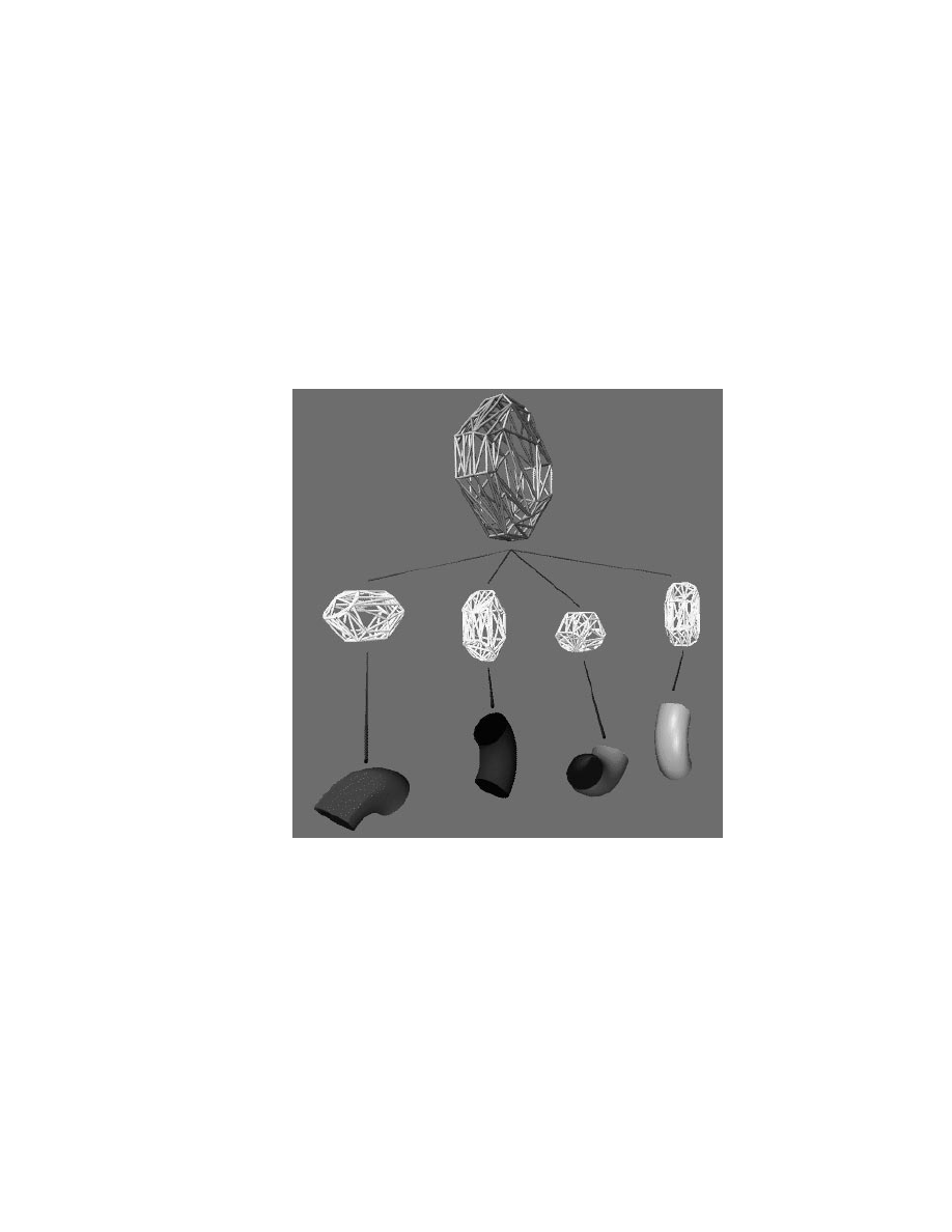
75
Figure 4.5: Hierarchical representation of a torus composed of Bezier surfaces

76
can have more than one closest feature at any time. As a result, local optimization
methods highlighted in the previous sections may not work for the non-convex objects.
The problem of collision detection between two Bezier surfaces is solved by
nding all the solutions to the equations (4.5) and (4.7). A real solution in the domain
to those equations implies a geometric collision and a precise contact between the
models. The algebraic method based on resultants and eigenvalues is used to nd all
the solutions to the equations (4.5) and (4.7) [55]. This global root nder is used when
the control polytopes of two Bezier surfaces collide. At that instant the two surfaces
may or may not have a geometric contact. It is possible that all the solutions to these
equations are complex. The set of equations in (4.5) represents an overconstrained
system and may have no solution in the complex domain as well. However, we apply
the algebraic method to the rst four equations in (4.5) and compute all the solutions.
The total number of solutions of a system of equations is bounded by the
Bezout bound. The resultant method computes all these solutions. As the objects
move, we update the coecients of these equations based on the rigid motion. We
obtain a new set of equations corresponding to (4.5) and (4.7), whose coecients are
slightly dierent as compared to the previous set. All the roots of the new set of
equations are updated using Newton's method. The previous set of roots are used as
initial guesses. The overall approach is like
homotopy methods
[64], This procedure
represents an algebraic analog of the geometric coherence exploited in the earlier
section.
As the two objects move closer to each other, the imaginary components of
some of the roots start decreasing. Finally, a real collision occurs, when the imaginary
component of one of the roots becomes zero.
We do not have to track all the paths corresponding to the total number of
solutions. After a few time steps we only keep track of the solutions whose imaginary
components are decreasing. This is based on the fact that the number of closest
points is much lower than the Bezout bound of the equations.

77
Chapter 5
Interference Tests for Multiple
Objects
In a typical environment, there are moving objects and stationary obstacles
as well. Assume that there are
N objects moving around in an environment of M
stationary obstacles. Each of
N movingobjects is also considered as a moving obstacle
to the other moving objects. Keeping track of the distance for
0
@
N
2
1
A
+
NM pairs of
objects at all time can be quite time consuming, especially in a large environment. In
order to avoid unnecessary computations and to speed up the run time, we present two
methods: one assumes the knowledge of maximumacceleration and velocity, the other
purely exploits the spatial arrangement without any other information to reduce the
number of pairwise interference tests. For the scheduling scheme in which we assume
the dynamics (velocities, accelerations, etc.) is known, we rely on the fact that only
the object pairs which have a small separation are likely to have an impact within the
next few time instances, and those object pairs which are far apart from each other
cannot possibly come to interfere with each other until certain time. For spatial
tests to reduce the number of pairwise comparisons, we assume the environment is
rather sparse and the objects move in such a way that the geometric coherence can
be preserved, i.e. the assumption that the motion is essentially continuous in time
domain.

78
5.1 Scheduling Scheme
The algorithm maintains a queue (implemented as a heap) of all pairs of
objects that might collide (e.g. a pair of objects which are rigidly attached to each
other will not appear in the queue). They are sorted by lower bound on time to
collision; with the one most likely to collide (i.e. the one that has the smallest
approximate time to collision) appearing at the top of the heap. The approximation
is a lower bound on the time to collision, so no collisions are missed. Non-convex
objects, which are represented as hierarchy trees as described in Chapter 4, are treated
as single objects from the point of view of the queue. That is, only the roots of the
hierarchy trees are paired with other objects in the queue.
The algorithm rst has to compute the initial separation and the possible
collision time among all pairs of objects and the obstacles, assuming that the mag-
nitude of relative initial velocity, relative maximum acceleration and velocity limits
among them are given. After initialization, at each step it only computes the closest
feature pair and the distance between one object pair of our interests, i.e. the pair
of objects which are most likely to collide rst; meanwhile we ignore the other object
pairs until one of them is about to collide. Basically, the algorithm puts all the object
pairs to sleep until the clock reaches the \wakeup" time for the rst pair on top of
the heap. Wakeup time
W
i
for each object pair
P
i
is dened as
W
i
=
t
iw
+
t
0
where
t
iw
is the lower bound on the time to collision for each pair
P
i
for most situations
(with exceptions described in the next sub-section) and
t
0
is the current time.
5.1.1 Bounding Time to Collision
Given a trajectory that each moving object will travel, we can determine the
exact collision time. Please refer to [17] for more details. If the path that each object
travels is not known in advance, then we can calculate a lower bound on collision
time. This lower bound on collision time is calculated adaptively to speed up the
performance of dynamic collision detection.

79
Let
a
max
be an upper bound on the relative acceleration between any two
points
on any pair of objects. The bound
a
max
can be easily obtained from bounds on
the relative absolute linear
~a
lin
and relative rotational accelerations
~a
rot
and relative
rotational velocities
~!
r
of the bodies and their diameters:
~a
max
=
~a
lin
+
~a
rot
~r+~!
r
(
~!
r
~r) where r is the vector dierence between the centers of mass of two bodies. Let
d be the initial separation for a given pair of objects, and v
i
(where
~v
i
=
~v
lin
+
~!
r
~r)
the initial relative velocity of closest points on these objects. Then we can bound the
time
t
c
to collision as
t
c
=
q
v
2
i
+ 2
a
max
d
,
v
i
a
max
(5.1)
This is the minimum safe time that is added to the current time to give the
wakeup time for this pair of objects. To avoid a \Zeno's paradox" condition where
smaller and smaller times are added and the collision is never reached, we must add
a lower bound to the time increment. So rather than just adding
t
c
as derived above,
we added
t
w
= max(
t
c
;t
min
), where
t
min
is a constant (say 1 mSec or
1
FrameRate
) which
determines the eective time resolution of the calculation.
As a side note here, we would like to mention the fact that since we can
calculate the lower bound on collision time adaptively, we can give a fairly good
estimate of exact collision time to the precision in magnitude of
t
min
. In addition,
since the lower bound on time to collision is calculated adaptively for the object
most likely to collide rst, it is impossible for the algorithm to fail to detect an
interpenetration.
This can be done by modifying
t
min
, the eective time resolution, and the
user dened safety tolerance
according to the environment so as to avoid the case
where one object collides with the other between time steps.
is used because the
polyhedra may be actually shrunk by
amount to approximate the actual object.
Therefore, the collision should be declared when the distance between two convex
polytopes is less than 2
. This is done to ensure that we can always report a collision
or near-misses.

80
5.1.2 The Overall Approach
Our scheme for dynamic simulation using our distance computation algo-
rithm is an iterative process which continuously inserts and deletes the object pairs
from a heap according to their approximate time to collision, as the objects move in
a dynamic environment.
It is assumed that there is a function
A
i
(
t) given for each object, which
returns the object's pose at time
t, as a 4x4 matrix. Initially, all poses are determined
at
t = 0, and the distance calculation algorithm in Chapter 3 is run on all pairs of
objects that might collide. The pairs are inserted into the heap according to their
approximate time to collision.
Then the rst pair of objects is pulled o the queue. Its closest feature pair
at
t = 0 will be available, and the distance measuring algorithm from Chapter refdist
is run. If a collision has occurred and been reported, then the pair is re-inserted
in the queue with a minimum time increment,
t
min
. If not, a new lower bound on
time-to-collision for that pair is computed, and the pair is re-inserted in the queue.
This process is repeated until the wakeup time of the head of the queue exceeds the
simulation time.
Note that the lower bound on collision time is calculated adaptively for the
pair most likely to collide. Therefore, no collision can be missed. We will not need to
worry about those sleeping pairs (which will not collide before their wake-up time),
until the clock reaches the wake-up time
W
i
for each pair
P
i
.
This scheme described above can take care of all object pairs eciently so
that the distant object pairs wake up much less frequently. Thus, it reduces the run
time in a signicant way.
If no upper bounds on the velocity and acceleration can be assumed, in the
next section we propose algorithms which impose a bounding box hierarchy on each
object in the environment to reduce the naive bound of
0
@
N
2
1
A
pairwise comparisons
for a dynamic environment of
n objects. Once the object pairs' bounding boxes
already collide, then we can apply the algorithm described in Chapter 3 to perform

81
collision detection and to nd the exact contact points if applicable.
5.2 Sweep & Sort and Interval Tree
In the three-dimensional workspace, if two bodies collide then their projec-
tions down to the lower-dimensional
x
,
y;y
,
z;x
,
z hyperplanes must overlap as
well. Therefore, if we can eciently
update
their overlapping status in each axis or in
a 2-dimensional plane, we can easily eliminate the object pairs which are denitely
not in contact with each other. In order to quickly determine all object pairs over-
lapping in the lower dimensions, we impose a virtual bounding box hierarchy on each
body.
5.2.1 Using Bounding Volumes
To compute exact collision contacts, using a bounding volume for an in-
terference test is not sucient, but it is rather ecient for eliminating those object
pairs which are of no immediate interests from the point of collision
detection
. The
bounding box can either be spherical or rectangular (even elliptical), depending on
the application and the environment. We prefer spherical and rectangular volume
due to their simplicity and suitability in our application.
Consider an environment where most of objects are elongated and only a
few objects (probably just the robot manipulators in most situations) are moving,
then rectangular bounding boxes are preferable. In a more dynamic environment
like a vibrating parts feeder where all objects are rather \fat" [68] and bouncing
around, then spherical bounding boxes are more desirable. If the objects are con-
cave or articulated, then a subpart-hierarchical bounding box representation (similar
to subpart-hierarchical tree representation, with each node storing a bounding box)
should be employed. The reasons for using each type of the bounding volumes are as
follows.
Using a spherical bounding volume, we can precompute the box during the
preprocessing step. At each time step, we only need to update the center of each

82
spherical volume and get the minimum and maximum
x;y;z
,
coordinates almost
instantaneously by subtracting the measurement of radius from the coordinates of the
center. This involves only one vector-matrix multiplication and six simple arithmetic
operations (3 addition and 3 subtraction). However, if the objects are rather oblong,
then a sphere is a rather poor bounding volume to use.
Therefore, a rectangular bounding box emerges to be a better choice for
elogated objects. To impose a virtual rectangular bounding volume on an object
rotating and translating in space involves a recomputation of the rectangular bound-
ing volume. Recomputing a rectangular bounding volume is done by updating the
maximum and minimum
x;y;z
,
coordinates at each time instance. This is a simple
procedure which can be done at constant time for each body. We can update the
\min" and \max" by the following approaches:
Since the bounding boxes are convex, the maximum and minimum in the
x;y;z
,
coordinates must be the coordinates of vertices. We can use a modied
vertex-face
routine from the incremental distance computation algorithm described
in Chapter 3. We can set up 6 imaginary boundary walls, each of these walls is located
at the maximal and minimal
x;y;z
,
coordinates possible in the environment. Given
the previous bounding volume, we can update each vertex of the bounding volume
by performing only half of modied
vertex-face
test, since all the vertices are always
in the Voronoi regions of these boundary walls. We rst nd the nearest point on the
boundary wall to the previous vertex (after motion transformation) on the bounding
volume, then we verify if the nearest point on the boundary wall lies inside of the
Voronoi region of the previous vertex. If so, the previous vertex is still the extremal
point (minimum or maximum in
x;y, or z
,
axis). When a constraint is violated
by the nearest point on the face (wall) to the previous extremal vertex, the next
feature returned will be the neighboring
vertex
, instead of the neighboring edge. This
is a simple modication to the point-vertex applicability criterion routine. It still
preserves the properties of locality and coherence well. This approach of recomputing
bounding volume dynamically involves 6
point-vertex
applicability tests.
Another simple method can be used based on the property of convexity.
At each time step, all we need to do is to check if the current minimum (or max-

83
imum) vertex in
x
,
(or
y;z
,
)coordinate still has the smallest (or largest)
x
,
(or
y;z
,
)coordinate values in comparison to its neighboring vertices. By performing this
verication process recursively, we can recompute the bounding boxes at expected
constant rate. Once again, we are exploiting the temporal and geometric coherence
and the locality of convex polytopes. We only update the bounding volumes for the
moving objects. Therefore, if
all
objects are moving around (especially in a rather
unpredictable way), it's hard to preserve the coherence well and the update overhead
may slow down the overall computation.
But, we can speed up the performance of this approach by realizing that
we are only interested in one coordinate value of vertices for each update, say
x
coordinate while updating the minimum or maximum value in x-axis. Therefore,
there is no need to transform the other coordinates, say
y and z values, in updating
the
x extremal vertices during the comparison with neighboring vertices. Therefore,
we only need to perform 24 vector-vector multiplications. (24 comes from 6 updates
in minimumand maximum in
x;y;z
,
coordinates and each update involves 4 vector-
vector multiplications, assuming each vertex has 3 neighboring vertices.)
For concave and articulated bodies, we need to use a hierarchical bounding
box structure, i.e. a tree of bounding boxes. Before the top level bounding boxes
collide, there is no need to impose a bounding volume on each subpart or each link.
Once the collision occurs between the parent bounding boxes, then we compute the
bounding boxes for each child (subpart or linkage). At last we would like to briey
mention that in order to report \near-misses", we should \grow" the bounding boxes
by a small amount to ensure that we perform the exact collision detection algorithm
when two objects are about to collide,
not
after they collide.
Given the details of computing bounding volumedynamically,we will present
two approaches which use \sort and sweep" techniques and a geometric data struc-
ture to quickly perform intersection test on the real intervals to reduce the number
of pairwise comparison.

84
5.2.2 One-Dimensional Sort and Sweep
In computational geometry, there are several algorithms which can solve the
overlapping problem for
d-dimensional bounding boxes in O(nlog
d
,1
n+s) time where
s is the number of pairwise overlaps [31, 47, 80]. This bound can be improved using
coherence.
Let a one-dimensional bounding box be [
b;e] where b and e are the real
numbers representing the beginning and ending points. To determine all pairs of
overlapping intervals given a list of
n intervals, we need to verify for all pairs i and j
if
b
i
2
[
b
j
;e
j
] or
b
j
2
[
b
i
;e
i
], 1
i < j
n. This can be solved by rst sorting a list
of all
b
i
and
e
i
values, from the lowest to the highest. Then, the list is traversed to
nd all the intervals which overlap. The sorting process takes
O(nlogn) and O(n) to
sweep through a sorted list and
O(s) to output each overlap where s is the number
of overlap.
For a sparse and dynamic environment, we do not anticipate each body to
make a relatively large movement between time steps, thus the sorted list should not
change much. Consequently the last sorted list would be a good starting point to
continue. To sort a \nearly sorted" list by
bubble sort
or
insertion sort
can be done
in
O(n + e) where e is the number of exchanges.
All we need to do now is to keep track of \status change", i.e. from overlap-
ping in the last time step to non-overlapping in the current time step and vise versa.
We keep a list of overlapping intervals at all time and update it whenever there is a
status change. This can be done in
O(n + e
x
+
e
y
+
e
z
) time, where
e
x
;e
y
;e
z
are the
number of exchanges along the
x;y;z-coordinate. Though the update can be done in
linear time,
e
x
;e
y
;e
z
can be
O(n
2
) with an extremely small constant. Therefore, the
expected
run time is linear in the total number of vertices.
To use this approach in a three-dimensional workspace, we pre-sort the mini-
mum and maximumvalues of each object along the
x;y;z
,
axis (as if we are imposing
a virtual bounding box hierarchy on each body), sweep through each nearly sorted list
every time step and update the list of overlapping intervals as we mentioned before.
If the environment is sparse and the motions between time frames are \smooth", we

85
expect the extra eort to check for collision will be negligible. This \pre-ltering"
process to eliminate the pairs of objects
not
likely to collide will run essentially in
linear time. A similar approach has been mentioned by Bara in [48].
This approach is especially suitable for an environment where only a few
objects are moving while most of objects are stationary, e.g. a virtual walk-through
environment.
5.2.3 Interval Tree for 2D Intersection Tests
Another approach is to extend the one-dimensional sorting and sweeping
technique to higher dimensional space. However, as mentioned earlier, the time bound
will be worse than
O(n) for two or three-dimensional sort and sweep due to the
dicultyto make a tree structure dynamicand exible for quick insertion and deletion
of a higher dimensional boxes. Nevertheless, for more dense or special environments
(such as a mobile robot moving around in a room cluttered with moving obstacles,
such as people), it is more ecientto use an interval tree for 2-dimensional intersection
tests to reduce the number of pairwise checks for overlapping. We can signicantly
reduce the extra eort in verifying the exchanges checked by the one-dimensional sort
and sweep. Here we will briey describe the data structure of an interval tree and
how we use it for intersection test of 2-dimensional rectangular boxes.
An interval tree is actually a
range tree
properly annotated at the nodes for
fast search of real intervals. Assume that
n intervals are given, as [b
1
;e
1
]
;
;[b
n
;e
n
]
where
b
i
and
e
i
are the endpoints of the interval as dened above. The range tree
is constructed by rst sorting all the endpoints into a list (
x
1
;
;x
m
) in ascending
order, where
m
2
n. Then, we construct the range tree top-down by splitting the
sort list
L into the left subtree L
l
and the right subtree
L
r
, where
L
l
= (
x
1
;
;x
p
)
and
L
r
= (
x
p
+1
;
;x
m
). The root has the split value
x
p
+
x
p+1
2
. We construct the
subtrees within each subtree recursively in this fashion till each leave contains only
an endpoint. The construction of the range tree for
n intervals takes O(nlogn) time.
After we construct the range tree, we further link all nodes containing stored intervals
in a doubly linked list and annotate each node if it or any of its descendant contains

86
stored intervals. The embellished tree is called the
interval tree
.
We can use the interval tree for static query, as well as for the rectangle
intersection problem. To check for rectangle intersection using the sweep algorithm:
we take a sweeping line parallel to the
y axis and sweep in increasing x direction, and
look for overlapping
y intervals. As we sweep across the x axis, y intervals appears
or disappear. Whenever there is an appearing
y interval, we check to see if the new
interval intersects the old set of intervals stored in the interval tree, report all intervals
it intersects as rectangle intersection, and add the new interval to the tree.
Each query of interval intersection takes
O(logn + k) time where k is the
number of reported intersection and
n is the number of intervals. Therefore, reporting
intersection among
n rectangles can be done in O(nlogn + K) where K is the total
number of intersecting rectangles.
5.3 Other Approaches
Here we will also briey mention a few dierent approaches which can be
used in other environments or applications.
5.3.1 BSP-Trees and Octrees
One of the commonly used tree structure is BSP-tree (binary space parti-
tioning tree) to speed up intersection tests in CSG (constructive solid geometry) [83].
This approach construct a tree from separating planes at each node recursively. It
partitions each object into groups of parts which are close together in binary space.
When, the separation planes are chosen to be aligned with the coordinate axes, then
a BSP tree becomes more or less like an octree.
One can think of an octree as tree of cubes within cubes. But, the size of the
cube varies depending on the number of objects occupying that region. A sparsely
populated region is covered by one large cube, while a densely occupied region is
divided into more smaller cubes. Each cube can be divided into 8 smaller cubes if
necessary. So, each node in the tree has 8 children (leaves).

87
Another modied version of BSP-Tree proposed by Vanecek [37] is a multi-
dimensional space partitioning tree called
Brep-Index
. This tree structure is used for
collision detection [10] between moving objects in a system called
Proxima
developed
at Prudue University.
The problem with tree structures is similar to that of using 2-d interval tree
that its update (insertion and deletion) is inexible and cumbersome, especially for
a large tree. The overhead of insertion and deletion of a node in a tree can easily
dominate the run time, especially when a collision occurs. The tree structures also
cannot capture the temporal and spatial coherence well.
5.3.2 Uniform Spatial Subdivision
We can divide the space into unit cells (or volumes) and place each object
(or bounding box) in some cell(s) [68]. To check for collisions, we have to examine the
cell(s) occupied by each box to verifyif the cell(s) is(are) shared by other objects. But,
it is dicult to set a near-optimal size for each cell and it requires tremendous amount
of allocated memory. If the size of the cell is not properly chosen, the computation
can be rather expensive. For an environment where almost all objects are of uniform
size, like a vibrating parts feeder bowl or molecular modeling [85, 68], this is a rather
ideal algorithm, especially to run on a parallel-computing machine. In fact, Overmars
has shown that using a hash table to look up an enetry, we can use a data structure
of O(n) storage space to perform the point location queries in constant time [68].
5.4 Applications in Dynamic Simulation and Vir-
tual Environment
The algorithms presented in this chapter have been utilized in dynamic
simulation as well as in a walk-through environment. These applications attest for
the practicality of the algorithms and the importance of the problem natures.
The algorithm described in Sec. 5.1 and the distance computation algorithm
described in Chapter 3 have been used in the dynamics simulator written by Mirtich

88
[62]. It reduces the frequency of the collision checks signicantly and helps to speed up
the calculations of the dynamic simulator considerably. Our vision of this dynamic
simulator is the ability to to simulate thousands of small mechanical parts on a
vibrating parts feeder in real time. Looking at our current progress, we believe such
a goal is attainable using the collision detection algorithms described in this thesis.
At the same time, the algorithm described in Sec. 5.2.2 is currently under
testing to be eventually integrated into a Walk-Through environment developed at
the University of North Carolina, Chapel Hill on their in-house Pixel Plane machine
[24]. In a virtual world like \walk-through environment" where a human needs to
interact with his/her surrounding, it is important that the computer can simulate
the interactions of the human participants with the passively or actively changing
environment. Since the usual models of \walk-through" are rather complex and may
have thousands of objects in the world, an algorithm as described in Sec. 5.2.2 becomes
an essential component to generate a realism of motions.

89
Chapter 6
An Opportunistic Global Path
Planner
The algorithm described in Chapter 3 is a key part of our general planning
algorithm presented in this chapter. This path planning algorithm creates an one-
dimensional roadmap of the free space of a robot by tracing out curves of maximal
clearance from obstacles. We use the distance computation algorithm to incrementally
compute distances between the robot pieces and the nearby obstacles. From there
we can easily compute gradients of the distance function in conguration space, and
thereby nd the direction of the maximal clearance curves.
This is done by rst nding the pairs of closest features between the robot
and the obstacles, and then keeping track of these closest pairs incrementally by calls
to this algorithm. The curves traced out by this algorithm are in fact maximally
clear of the obstacles. As mentioned earlier, once a pair of initialization features
in the vicinity of the actual closest pair is found, the algorithm takes a very short
time (usually constant) to nd the actual closest pair of features. Given the closest
features, it is straight forward to compute the gradient of the distance function in
conguration space which is what we need to trace the skeleton curves.
In this chapter, we will describe an opportunistic global path planner which
uses the opportunistic local method (Chapter 3) to build up the one-dimensional
skeleton (or freeway) and global computation to nd the critical points where linking

90
curves (or bridges) are constructed.
6.1 Background
There have been two major approaches to motion planning for manipulators,
(i) local methods, such as articial potential eld methods [50], which are usually fast
but are not guaranteed to nd a path, and (ii) global methods, like the rst Roadmap
Algorithm [18], which is guaranteed to nd a path but may spend a long time doing
it. In this chapter, we present an algorithm which has characteristics of both. Our
method is an incremental construction of a skeleton of free-space. Like the potential
eld methods, the curves of this skeleton locally maximizesa certain potential function
that varies with distance from obstacles. Like the Roadmap Algorithm, the skeleton,
computed incrementally, is eventually guaranteed to contain a path between two
congurations if one exists. The size of the skeleton in the worst case, is comparable
with the worst-case size of the roadmap.
Unlike the local methods, our algorithm never gets trapped in local extremal
points. Unlike the Roadmap Algorithm, our incremental algorithm can take advan-
tage of a non-worst-case environment. The complexity of the roadmap came from
the need to take recursive slices through conguration space. In our incremental
algorithm, slices are only taken when an initial search fails and there is a \bridge"
through free space linking two \channels". The new algorithm is no longer recursive
because bridges can be computed directly by hill-climbing . The bridges are built
near \interesting" critical points and inection points. The conditions for a bridge
are quite strict. Possible candidate critical points can be locally checked before a slice
is taken. We expect few slices to be required in typical environments.
In fact, we can make a stronger statement about completeness of the algo-
rithm. The skeleton that the algorithm computes eventually contains paths that are
homotopic to all paths in free space. Thus, once we have computed slices through
all the bridges, we have a complete description of free-space for the purposes of path
planning. Of course, if we only want to nd a path joining two given points, we stop
the algorithm as soon as it has found a path.

91
The tracing of individual skeleton curves is a simple enough task that we
expect that it could be done in real time on the robot's control hardware, as in other
articial potential eld algorithms. However, since the robot may have to backtrack
to pass across a bridge, it does not seem worthwhile to do this during the search.
For those readers already familiar with the Roadmap Algorithm, the follow-
ing description may help with understanding of the new method: If the conguration
space is
R
k
, then we can construct a hypersurface in
R
k
+1
which is the graph of the
potential function, i.e. if
P(x
1
;:::;x
k
) is the potential, the hypersurface is the set
of all points of the form (
x
1
;:::;x
k
;P(x
1
;:::;x
k
)). The skeleton we dene here is a
subset of a roadmap (in the sense of [18]) of this hypersurface.
This work builds on a considerable volume of work in both global motion
planning methods [18] [54], [73], [78], and local planners, [50]. Our method shares a
common theme with the work of Barraquand and Latombe [6] in that it attempts to
use a local potential eld planner for speed with some procedure for escaping local
maxima. But whereas Barraquand and Latombe's method is a local method made
global, we have taken a global method (the Roadmap Algorithm) and found a local
opportunistic way to compute it.
Although our starting point was completely dierent, there are some other
similarities with [6]. Our \freeways" resemble the valleys intuitively described in [6].
But the main dierence between our method and the method in [6] is that we have
a guaranteed (and reasonably ecient) method of escaping local potential extremal
points and that our potential function is computed in the conguration space.
The chapter is organized as follows: Section 6.2 contains a simple and gen-
eral description of roadmaps. The description deliberately ignores details of things
like the distance function used, because the algorithm can work with almost any
function. Section 6.3 gives some particulars of the application of articial potential
elds. Section 6.4 describes our incremental algorithm, rst for robots with two de-
grees of freedom, then for three degrees of freedom. Section 6.5 gives the proof of
completeness for this algorithm.

92
6.2 A Maximum Clearance Roadmap Algorithm
We denote the space of all congurations of the robot as
CS. For example,
for a rotary joint robot with
k joints, the conguration space CS is
R
k
, the set of all
joint angle tuples (
1
;:::;
k
). The set of congurations where the robot overlaps some
obstacle is the conguration space obstacle
CO, and the complement of CO is the
set of free (non-overlapping) congurations
FP. As described in [18], FP is bounded
by algebraic hypersurfaces in the parameters
t
i
after the standard substitution
t
i
=
tan(
i
2
). This result is needed for the complexity bounds in [18] but we will not need
it here.
A roadmap is a one-dimensional subset of
FP that is guaranteed to be
connected within each connected component of
FP. Roadmaps are described in some
detail in [18] where it is shown that they can be computed in time
O(n
k
log
n(d
O
(
n
2
)
))
for a robot with
k degrees of freedom, and where free space is dened by n polynomial
constraints of degree
d [14]. But n
k
may still be too large for many applications, and
in many cases the free space is much simpler than its worst case complexity, which
is
O(n
k
). We would like to exploit this simplicity to the maximum extent possible.
The results of [6] suggest that in practice free space is usually much simpler than the
worst case bounds. What we will describe is a method aimed at getting a minimal
description of the connectivity of a particular free space. The original description of
roadmaps is quite technical and intricate. In this paper, we give a less formal and
hopefully more intuitive description.
6.2.1 Denitions
Suppose
CS has coordinates x
1
;:::;x
k
. A slice
CS
j
v
is a slice by the hy-
perplane
x
1
=
v. Similarly, slicing FP with the same hyperplane gives a set denoted
FP
j
v
. The algorithm is based on the key notion of a channel which we dene next:
A
channel-slice
of free space
FP is a connected component of some slice
FP
j
v
.

93
The term channel-slice is used because these sets are precursors to channels. To
construct a channel from channel slices, we vary
v over some interval. As we do this,
for most values of
v, all that happens is that the connected components of FP
j
v
change shape continuously. As
v increases, there are however a nite number of
values of
v, called
critical values
, at which there is some topological change. Some
events are not signicant for us, such as where the topology of a component of the
cross-section changes, but there are four important events: As
v increases a connected
component of
FP
j
v
may appear or disappear, or several components may join, or a
single component may split into several. The points where joins or splits occur are
called
interesting critical points
. We dene a channel as a maximal connected union
of cross sections that contains no image of interesting critical points. We use the
notation
FP
j
(
a;b
)
to mean the subset of
FP where x
1
2
(
a;b)
R
.
A
channel
through
FP is a connected component of FP
(
a;b
)
containing no
splits or joins, and (maximality) which is not contained in a connected component of
FP
(
c;d
)
containing no splits or joins, for (
c;d) a proper superset of (a;b). See Fig. 6.1
for an example of channels.
The property of no splits or joins can be stated in another way. A maximal
connected set
C
j
(
a;b
)
FP
j
(
a;b
)
is a channel if every subset
C
j
(
e;f
)
is connected for
(
e;f)
(
a;b).
6.2.2 The General Roadmap
Now to the heart of the method. A roadmap has two components:
(i) Freeways (called silhouette curves in [18]) and
(ii) Bridges (called linking curves in [18]).
A freeway is a connected one-dimensional subset of a channel that forms a backbone
for the channel. The key properties of a freeway are that it should span the channel,
and be continuable into adjacent channels. A freeway
spans
a channel if its range of
x
1
values is the same as the channels, i.e. a freeway for the channel
C
j
(
a;b
)
must have
points with all
x
1
coordinates in the range (
a;b). A freeway is
continuable
if it meets
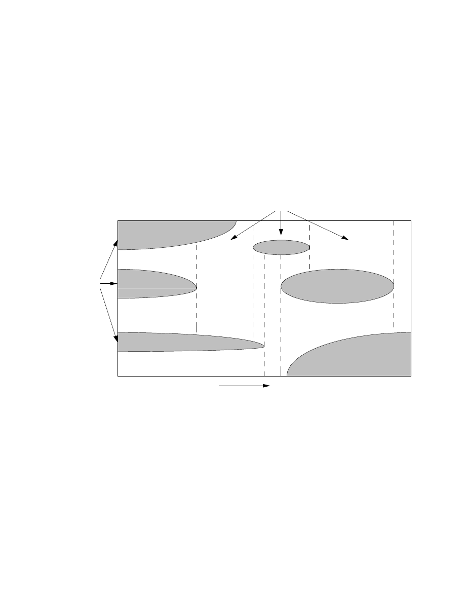
94
CO
Channels
x
1
Figure 6.1: A schematized 2-d conguration space and the partition of free space into
x
1
-channels.

95
another freeway at its endpoints. i.e. if
C
j
(
a;b
) and
C
0
j
(
b;c
)
are two adjacent channels,
the
b endpoint of a freeway of C
j
(
a;b
)
should meet an endpoint of a freeway of
C
0
j
(
b;c
)
.
(Technically, since the intervals are open, the word \endpoint" should be replaced by
\limit point")
In general, when a specic method of computing freeway curves is chosen,
there may be several freeways within one channel. For example, in the rest of this
chapter, freeways are dened using articial potential functions which are directly
proportional to distance from obstacles. In this case each freeway is the locus of local
maxima in potential within slices
FP
j
v
of
FP as v varies. This locus itself may have
some critical points, but as we shall see, the freeway curves can be extended easily
past them. Since there may be several local potential maxima within a slice, we may
have several disjoint freeway curves within a single channel, but with our incremental
roadmap construction, this is perfectly OK.
Now to bridges. A bridge is a one-dimensional set which links freeways from
channels that have just joined, or are about to split (as
v increases). Suppose two
channels
C
1
and
C
2
have joined into a single channel
C
3
, as shown in Fig. 6.2. We
know that the freeways of
C
1
and
C
2
will continue into two freeway curves in
C
3
.
These freeways within
C
3
are not guaranteed to connect. However, we do know that
by denition
C
3
is connected in the slice slice
x
1
=
v through the critical point, so
we add linking curves from the critical point to
some
freeway point in each of
C
1
and
C
2
. It does not matter which freeway point, because the freeway curves inside the
channels
C
1
and
C
2
must be connected within each channel, as we show in Sec. 6.5.
By adding bridges, we guarantee that whenever two channels meet (some points on)
their freeways are connected.
Once we can show that whenever channels meet, their freeways do also (via
bridges), we have shown that the roadmap, which is the union of freeways and bridges,
is connected. The proof of this very intuitive result is a simple inductive argument
on the (nite number of) channels, given in Sec. 6.5.
The basic structure of the general Roadmap Algorithm follows:
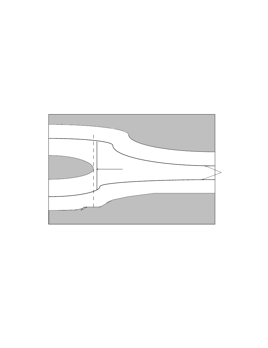
96
C
2
Bridge
Freeways
C
3
C
1
Figure 6.2: Two channels
C
1
and
C
2
joining the channel
C
3
, and a bridge curve in
C
3
.

97
1. Start tracing a freeway curve from the start conguration, and also from the
goal.
2. If the curves leading from the start and goal are not connected, enumerate a
split or join point, and add a bridge curve \near" the split or join (
x
1
-coordinate
of the slice slightly greater than that of the joint point for a join, slightly less
for a split).
3. Find all the points on the bridge curve that lie on other freeways, and trace
from these freeways. Go to step (2).
The algorithm terminates at step (2) when either the start and goal are connected,
in which case the algorithm signals success and returns a connecting path, or if it
runs out of split and join points, in which case there is no path connecting the start
and goal. This description is quite abstract, but in later sections we will give detailed
description of the approach in two- and three-dimensional conguration spaces.
Three things distinguish our new algorithm from the previous Roadmap
Algorithm. The most important is that the new algorithm is not recursive. Step 2
involves adding a bridge curve which is two pieces of curve found by hill-climbing on
the potential. In the original roadmap algorithm, linking curves had to be dened
recursively, because it is not possible to hill-climb to a maximum with an algebraic
curve. Another dierence is that the freeways do not necessarily lie near the boundary
of free space as they did in [18]. In our present implementation we are in fact using
maximum clearance freeways. But the most important dierence is that we now
only enumerate
true
split or join points. For a robot with
k degrees of freedom and
an environment of complexity
n, it can be shown that there are at most O(n
(
k
,1)
)
potential split or join points. (Please refer to Sec. proof.planner for the proof on
the upper bound for the maximum number of interesting critical points.) But many
experiments with implemented planners in recent years have shown that the number
of true splits or joins in typical conguration spaces is much lower. In our new
algorithm, we can make a purely local test on a potential split or join point to see
if it is really qualied. The vast majority of candidates will not be, so we expect far

98
fewer than
O(n
(
k
,1)
) bridges to be required.
Denition
A point
p in
R
k
+1
is an
interesting critical point
if for every neighborhood
U
of
p, one of the following holds:
(i) The intersection
U
\
x
,1
1
(
x
1
(
p) + ) consists of several connected components
for all suciently small
. This is a generalized split point.
(ii) The intersection
U
\
x
,1
1
(
x
1
(
p)
,
) consists of several components for all su-
ciently small
. This is a generalized join point.
We will assume the environment is generic, i.e. there is no special topology
such that a small perturbation will change the clearance of the paths. This is true for
almost all practical situations: most obstacles have a reasonably large interior space
that a small perturbation will not aect much of the obstacle conguration space.
Based on the transversality condition of general position assumptions in [18], the
interesting critical points can be computed as follows. Let
S be the set of equations
used to calculate the critical points. The set
S is dened by inequalities, and its
boundary is a union of surfaces of various dimensions. Let
S
be such a surface; it
will be dened as the intersection of several conguration space constraint surfaces.
Each of these is given by an equation of the form
f
i
= 0. To nd the critical points
of such a surface w.r.t. the function
x
1
(
:), we rst dene a polynomial g as follows:
g =
l
X
i
=1
f
2
i
(6
:1)
and then solve the system
g = ; @
@x
2
g = 0
@
@x
k
g = 0
(6
:2)
where
l is the number of equations which are zero on S
, the
x
2
;:::;x
k
are coordinates
which are orthogonal to
x
1
, and
is an innitesimal that is used to simplify the
computation (see [18]).
It can be shown [21] that the solutions of interest can be recovered from the
lowest degree coecient in
of the resultant of this system. This normally involves

99
computing a symbolic determinant which is a polynomial in
[57]. But a more
practical approach is to recover only the lowest coecient in
by using straight line
program representations and dierentiating [33].
To enumerate all the interesting critical points is computationally expensive,
since we have to solve
O(n
(
k
,1)
) systems of non-linear equations. Thus, we also plan
to experiment with randomly chosen slice values in some bounded ranges, alternating
with slices taken at true split or join points. The rationale for this is that in practice
the \range" of slice values over which a bridge joins two freeways is typically quite
large. There is a good probability of nding a value in this range by using random
values. Occasionally there will be a wide range of slice values for a particular bridge,
but many irrelevant split and join points may be enumerated with values outside this
range. To make sure we do not make such easy problems harder than they should be,
our implementation alternates slices taken near true split and join points with slices
taken at random
x
1
values.
6.3 Dening the Distance Function
The idea of our approach is to construct a potential eld which repels the
point robot in conguration space away from the obstacles. Given a goal position
and a description of its environment, a manipulator will move along a \maximum
potential" path in an \articial potential eld". The position to be reached represents
a critical point that will be linked by the
bridge
to the nearest maximum, and the
obstacles represent repulsive surfaces for the manipulator parts.
Let
CO denote the obstacles, and x the position in
R
k
. The articial po-
tential eld
U
art
(
x) induces an articial repulsion from the surface of the obstacles.
U
art
(
x) is a non-negative function whose value tends to zero as any part of the robot
approaches an obstacle. One of the classical analytical potential elds is the Euclidean
distance function.
Using the shortest distance to an obstacle
O, we have proposed the following
potential eld
U
art
(
x):

100
U
art
(
x) = min
ij
(
D(O
i
;L
j
(
x)))
where
D(O
i
;L
j
(
x)) is the shortest Euclidean distance between an obstacle O
i
and
the link
L
j
when the robot is at conguration
x. D(O
i
;L
j
(
x)) is obtained by a local
method for fast computation of distance between convex polyhedra in Chapter 3.
Notice that the proposed
U
art
(
x) is not a continuously dierentiable function
as in many potential eld methods.
U
art
(
x) is
piecewise
continuous and dierentiable.
This is perfectly all right for the application in our Roadmap algorithm. In fact it
will be a lower envelope of smooth functions. This is all the better because it means
that local maxima that do not occur where the function is smooth are all the more
sharply dened. The graph of the distance function certainly has a
stratication
into
a nite number of smooth pieces [87]. Its maxima will be the union of certain local
maxima of these smooth pieces. So we can still use the system of equations dened
earlier to nd them.
With this scheme, a manipulator moves in such a way to maximize the
articial potential eld
U
art
(
x). But like any local method, just following one curve
of such maxima is not guaranteed to reach the goal. Thus, the need for bridges.
6.4 Algorithm Details
The algorithm takes as input a geometric description of the robot links
and obstacles as convex polyhedra or unions of convex polyhedra. It also takes the
initial and goal congurations, and the kinematic description of the robot, say via
Denavit-Hartenberg parameters. The output is a path between the initial and goal
congurations represented as a sequence of closely spaced points (more closely than
the C-space distance to the nearest obstacle at that point), assuming such a path
exists. If there is no path, the algorithm will eventually discover that, and output
\NO PATH".
The potential function is a map
U
art
:
CS
!
R
. The graph of the function
is a surface in
CS
R
. Let
u and v denote two coordinate axes, the Roadmap

101
Algorithm xes
v and then follows the extremal points in direction u as the value of
v varies. But, the new algorithm diers from the original roadmap algorithm[18] in
the following respects:
It does not always construct the entire roadmap
In the new algorithm,
v = x
i
, where
x
i
is one of the CS coordinates while
u = h,
where
h is the height of the potential function. Yet, in the original, v = x
i
and
u = x
j
where
x
i
and
x
j
are
both
CS coordinates.
The original Roadmap algorithm xes the
x
i
coordinate and follows extremal
points (maxima, minima and saddles) in
x
j
, to generate the silhouette curves.
On the other hand, the new algorithm xes
x
i
, and follows only
maxima
in
h.
The new algorithm is not recursive. Recursion was necessary in the original
because there is no single algebraic curve that connects an arbitrary point to
an extremum in
u. But the new algorithm uses numerical hill-climbing which
has no such limitation.
6.4.1 Freeways and Bridges
A roadmap has two major components { freeways and bridges. They are
generated as following:
Freeway Tracing
is done by tracking the locus of local maxima in distance within
each slice normal to the sweeping direction. Small steps are made in the sweep
direction, and the local maxima recomputed numerically. Freeway tracing con-
tinues in both directions along the freeway until it terminates in one of two
ways:
(a) The freeway runs into an inection point, a point where the curve tangent
becomes orthogonal to the sweep direction. It is always possible to continue
past these points by adding a bridge.
(b) The freeway runs into an obstacle. This is a normal termination, and the
tracing simply stops and the algorithm backtracks.

102
Bridges
begin always at inection points or critical points and terminate always at
freeway points within the same slice. The algorithm simply follows the gradient
of the potential function from the start point within the slice until it reaches a
local maximum, which must be a freeway point.
Enumeration of Critical Points
Critical points are calculated as in Section 2. But most of these critical
points will not be interesting. We can check locally among all the critical points
to see if they qualify to be a \split" or \join". This test checks if the point has a
neighborhood that is \saddle-like". It is based on the orientations of the CSpace
boundary surface normals at the critical point.
Random Slicing
Optionally, the user may wish to add roadmaps of randomly chosen slices,
rather than calculating many critical points (or rather than calculating them at all,
but then of course, completeness will be lost). This
is
a recursive procedure, and
involves choosing a
v value at random, making a recursive call to the algorithm on
this
v-slice.
Random slicing may also be used within the slice itself, and so on, which
leads to a depth-
k recursion tree. If this is done, some search heuristics must be added
to guide the choice of where in the tree the next slice (and hence the next child) should
be added. The heuristic also needs to trade o random slicing and critical point
enumeration. The goal of the heuristic is to enumerate enough random slices that
the algorithm will have a good chance of success on \easy" environments (intuitively
where there are large passages between channels) without having to explore too many
critical points. Yet it should still nd its way around a dicult environment using
the critical slices without having wasted most of its time taking random slices.
Given the general outline of our algorithm, we will now give an instantiation
on 2-D and a detailed description of how it can be applied to 3-D.
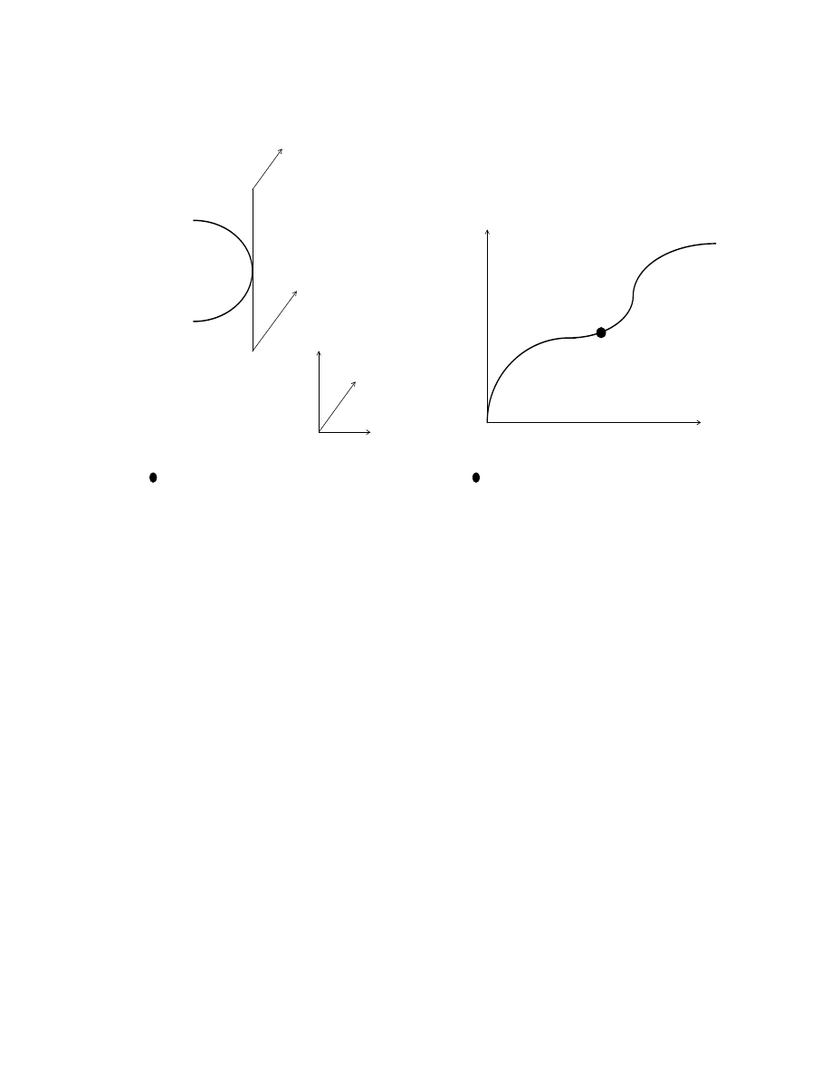
103
y
R
x = x
0
P
inflect
x
y
R
Portion of silhouette curve in CS x R
Slice projection at x = x
0
in R-y plane
P
inflect
Figure 6.3: A pictorial example of an inection point in
CS
R
vs. its view in
R
y
at the slice
x = x
0
6.4.2 Two-Dimensional Workspace
Starting from the initial position
p
init
2
CS, we rst x one of the axes of
CS and then take the x coordinate of a slice to be the x coordinate of p
init
. Then we
search this slice to nd the nearest local maximum. (This local maximumis a freeway
point.) Next, we build a
bridge
between the point
p
init
and this local maximum. At
the same time, we begin tracing a freeway curve from the goal. If the goal is not on
the maximum contour of the potential eld, then we must build a
bridge
to link it to
the nearest local maximum. Afterwards, we trace the locus of this local maximum as
x varies until we reach an endpoint. If the current position p
loc
on the curve is the goal
G, then we can terminate the procedure. Otherwise, we must verify whether p
loc
is a
\dead-end" or an inection point of the slice
x = x
0
. (See Fig. 6.3.) If
p
loc
is a point
of inection, then we can continue the curve by taking a slice at the neighborhood of
the inection point and hill-climbing along the gradient direction
near
the inection
point. This search necessarily takes us to another local maximum.

104
Fig. 6.4 demonstrates how the algorithm works in 2-d
CS. This diagram is
a projection of a constructed potential eld in
CS x
R
onto the
x-y plane of the 2-d
CS. The shaded area is the CO in the conguration space. The solid curves represent
the contour of maximum potential, while the dashed curves represent the minima.
Furthermore, the path generated by our planner is indicated by arrows. In addition,
the vertical lines symbolize channel slices through the interesting critical points and
inection points. When this procedure has been taken to its conclusion and both
endpoints of the freeway terminate at dead-ends, then at this point it is necessary to
take a slice at some value of
x. Our planner generates several random x-values for
slices (at a uniformly spaced distribution along the span of the freeway), interweaving
them with an enumeration of all the interesting critical points. If after a specied
number of random values, our planner fails to nd a connecting path to a nearby
local maximum, then it will take a slice through an interesting critical point. Each
slice, being 1-dimensional, itself forms the bridge curve (or a piece of it does). We
call this procedure repeatedly until we reach the goal position
G or have enumerated
all the interesting critical points.
The algorithm is described schematically below:
Algorithm
Procedure FindGoal (Environment,
p
init
, G)
if (
p
init
6
=
G)
then Explore(
p
init
) and Explore(
G)
else return(FoundGoal);
even := false;
While ( CritPtRemain and NotOnSkeleton(G) ) do
if (even)
then x := Random (x-range)
else x := x-coord(next-crit-pt());
TakeSlice(x);
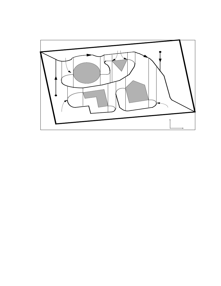
105
P
init
Boundary
Boundary
y
x
G
Silhouette
(freeway)
Bridge
Inflection Point
Inflection Point
Critical Points
Critical Point
Figure 6.4: An example of the algorithm in the 2-d workspace
even := not even;
end(while);
End(FindGoal);
Function Explore(p)
% Trace out a curve from p
q := search-up&down(p);
% To move up & down only in
y, using gradient near p
if new(q) then
% new() checks if q is already on the curve
begin(if)
<e1,e2> := trace(q);
% trace out the curve from q, output two end points
if inection(e1) then Explore(e1);

106
if inection(e2) then Explore(e2);
% inection(p) checks if p is an inection point
end(if);
End(Explore);
Function TakeSlice(x-coordinate(p))
% This function generates all points on the slice and explore
% all the maxima on the slice.
old-pt := nd-pt(x-coordinate);
% nd-pt() nd all the points on the x-coordinate.
% It moves up&down until reaches another maximum.
new-pt := null;
For (each pt in the old-pt) do
<up,down> := search-up&down(pt);
%
<up,down> is a pair of points of 0,1,or2 pts
new-pt := new-pt +
<up,down>;
For (each pt in the new-pt) do
Explore(pt);
End(TakeSlice);
6.4.3 Three-Dimensional Workspace
For a three-dimensional workspace, the construction is quite similar. Start-
ing from the initial position
p
init
and the goal
G, we rst x one axis, X. We trace
from the start point to a local maximum of distance within the
Y -Z plane containing
the start point. Then we follow this local maximum by taking steps in
X. If this
curve terminates in an inection point, we can always reach another maximum by
following the direction of the potential gradient
just beyond
the inection point in
X.
Eventually, though, we expect to terminate by running into an obstacle.

107
When we wish to enumerate a critical point, the bridge curve is the same
as the rst segment that we used to get from
p
init
onto the freeway. That is, we
trace from the critical point along the direction of the gradient within the current
Y -Z slice. There will be two directions outward from the critical point along which
the distance increases. We follow both of these, which gives us a bridge curve linking
freeways of two distinct channels.
If we decide to use random slicing, we select a slice
FP
j
x
normal to the
x-
axis and call the algorithm of the last section on that slice. We require it to produce a
roadmap containing any freeway points that we have found so far that lie in this slice.
This algorithm itself may take random slices, so we need to limit the total number of
random slices taken before we enumerate the next interesting critical point (in 3-D),
so that random slicing does not dominate the running time.
6.4.4 Path Optimization
After the solution path is obtained, we plan to smooth it by the classical
principles of variational calculus, i.e. to solve a classical two points boundary value
problem. Basically we minimize the potential which is a function of both distance
and smoothness to nd a
locally
optimal (smooth) path.
Let
s be the arc that is the path rened from a sequence of points between
a and b in space, r be the shortest Euclidean distance between the point robot and
the obstacle, and
be the curvature of the path at each point. The cost function for
path optimization that we want to minimize is:
f(s;r;) =
Z
b
a
(Ar
2
+
B
2
)
ds
where
r, , and s are functions of a point P
i
in a given point sequence, and
A;B are
adjustment constants. Taking the gradient of this function with respect to each point
P
i
gives us the direction of an improved,
locally
optimal path.
This can be done in the following manner: given a sequence of points
(
P
1
;P
2
;
;P
k
), we want to minimize the cost function

108
g(P
i
) =
X
i
A
r(P
i
)
2
j
S
i
j
+
B(P
i
)
2
j
S
i
j
(6.3)
where
S
i
and
(P
i
) are dened as:
S
i
= P
i
+1
,
P
i
,1
2
(P
i
) =
\
P
i
,1
;P
i
;P
i
+1
j
S
i
j
Now, taking the gradient w.r.t.
P
i
, we have
r
g(P
i
) =
X
i
,
2
A
r(P
i
)
3
r
r(P
i
)
j
S
i
j
+ 2
B(P
i
)
r
(P
i
)
j
S
i
j
(6.4)
The most expensive procedure in computing the above gradient is to com-
pute the distance at each point. By using the incremental distance calculation algo-
rithm described in Chapter 3, we can compute the distance between the robot and the
closest obstacle in constant time. Since we have to do this computation for a sequence
of points, the computation time for each iteration to smooth the curve traced out by
our planner is linear in the total number of points in a given sequence. After several
iterations of computing the gradient of the summation in Eqn.6.4, the solution path
will eventually be smooth and
locally
optimal.
6.5 Proof of Completeness for an Opportunistic
Global Path Planner
Careful completeness proofs for the roadmap algorithm are given in [18] and
[19]. These proofs apply with very slight modication to the roadmap algorithm that
we describe in this paper. The roadmap of [18] is the set of extremal points in a certain
direction in free space. Therefore it hugs the boundary of free space. The roadmap
described in this paper follows extrema of the
distance function
, and therefore stays
well clear of obstacles (except at critical points). But in fact the two are very similar

109
if we think of the
graph of the distance function
in
R
n
. This is a surface
S in
R
(
n
+1)
and if we follow the extrema of distance on this surface, the roadmap of this paper is
exactly a roadmap in the sense of [18] and [19].
The silhouette curves of [18] correspond to the freeway curves of this paper,
and the linking curves correspond to bridges. Recall the basic property required of
roadmaps:
Denition
A subset of
R of a set S satises the
roadmap condition
if every connected
component of
S contains a single connected component of R.
For this denition to be useful, there is an additional requirement that any
point in
S can \easily" reach a point on the roadmap.
There is one minor optimization that we take advantage of in this paper.
That is to trace only
maxima
of the distance function, rather than both maxima and
minima. This can also be applied to the original roadmap.
For those readers not familiar with the earlier papers, we give here an infor-
mal sketch of the completeness proof. We need some notation rst.
Let
S denote the surface in
R
(
n
+1)
which is the graph of the distance function.
S is an n-dimensional set and is semi-algebraic if conguration space is suitably
parametrized. This simply means that it can be dened as a boolean combination of
inequalities which are polynomials in the conguration space parameters.
One of the coordinates in conguration space
R
n
becomes the
sweep direc-
tion
. Let this direction be
x
1
. Almost any direction in
CS will work, and heuristics
can be used to pick a direction which should be good for a particular application.
When we take slices of the distance surface
S, they are taken normal to the x
1
co-
ordinate, so
S
j
a
means
S
\
(
x
1
=
a). Also, for a point p in
R
(
n
+1)
,
x
1
(
p) is the
x
1
-coordinate of
p.
The other coordinate we are interested in is the distance itself, which we
think of as the height of the distance surface. So for a point
p in
R
(
n
+1)
,
h(p) is the
value of the distance at this conguration.

110
For this paper, we use a slightly dierent denition of silhouettes, taking only
local maxima into account. We will assume henceforth that the conguration space is
bounded in every coordinate. This is certainly always the case for any practical robot
working in a conned environment, such as industrial robot manipulators, mobile
robots, etc. If it is not bounded, there are technical ways to reduce to a bounded
problem, see for example [14]. The set of free congurations is also assumed to be
closed. The closed and bounded assumptions ensure that the distance function will
attain locally maximal values on every connected component of free space.
A
silhouette point
is a locally maximal point of the function
h(:) on some
slice
S
j
a
of
S. The
silhouette
(
S) of S is the set of all such points for all a.
The key properties of the silhouette are ([18], [19]):
(i) Within each slice of
S, each connected component of S
j
a
must contain at least
one silhouette point.
(ii) The silhouette should be one-dimensional.
(iii) The critical points of the silhouette w.r.t the function
x
1
(
:) should include the
critical points of the set
S.
Clearly, using local maxima will satisfy property (i). This is true simply
because a continuous function (in this case, a distance function with the value zero
on the boundary and positive values in the interior) has a local maximumin a compact
set. For property (ii) we require that the directions
x
1
and
h be \generic" (see the
earlier papers). This is easily done by picking a general
x
1
, but
h may not be generic
a priori. However, rather than the true distance
h, we assume that the distance
plus a very small linear combination of the other coordinates is used. This linear
combination can be arbitrarily small, and we assume that it is small enough that it
does not signicantly aect the clearance of silhouette points.
For property (iii), we depart somewhat from the original denition. The
critical points of the silhouette curves that we have traced can be discovered during
the tracing process (they are the points where the curve tangent becomes orthogo-
nal to
x
1
). But we need to nd all (or a sucient set of) critical points to ensure

111
completeness. All critical points do indeed lie on silhouette curves, but since our
algorithm is incremental, we may not discover these other curves unless we encounter
points on them. So we need a systematic way to enumerate the critical points of
S,
since these will serve as starting points for tracing the silhouette curves that we need
for completeness.
In fact, not all critical points of
S are required. There is a subset of them
called
interesting critical points
that are sucient for our purpose. Intuitively, the
interesting critical points are the split or join points in higher dimensions. They can
be dened as follows:
Denition
A point
p in
R
k
+1
is an
interesting critical point
if for every neighborhood
U
of
p, one of the following holds:
(i) The intersection
U
\
x
,1
1
(
x
1
(
p) + ) consists of several connected components
for all suciently small
. This is a generalized split point.
(ii) The intersection
U
\
x
,1
1
(
x
1
(
p)
,
) consists of several components for all su-
ciently small
. This is a generalized join point.
From the denition above, it follows that as we sweep the plane
x
1
=
a
through
S, the number of connected components of S
j
a
changes only when the plane
passes though interesting critical points.
Denition
Now we can dene the roadmap of the surface
S. The roadmap R(S) is
dened as follows: Let
P
C
(
S) be the set of interesting critical points of x
1
(
:) on S,
P
C
() be the set of critical points of
x
1
(
:) on the silhouette, and P
C
the union of
these two. The roadmap is then:
R(S) = (S)
[
(
[
p
2
P
c
L(p))
(6
:5)
That is, the roadmap of
S is the union of the silhouette (S) and various linking
curves
L(p). The linking curves join critical points of S or to other silhouette
points.

112
The new roadmap algorithm has an advantage over the original in that
it is not restricted to algebraic curve segments. This is because the original was
formulated to give precise algorithmic bounds on the planning problem, whereas the
new algorithm approximates the silhouette by tracing. Tracing is just as easy for
many types of non-algebraic curves as for algebraic ones.
This allows us to do linking in a single step, whereas algebraic linking curves
must be dened recursively. We generate linking curves in the present context by
simply xing the
x
1
coordinate and hill-climbing to a local maximum in
h(:). The
curve traced out by the hill-climbing procedure starts at the critical point and ends
at a local maximum(which will be a silhouette point) of the distance within the same
x
1
slice. Thus it forms a linking curve to the silhouette. If we are at an interesting
critical point, there will be two opposing directions (both normal to
x
1
) along which
the distance function increases. Tracing in both directions links the critical point to
silhouette points on both channels that meet at that critical point.
Theorem
R(S) satises the roadmap condition.
Proof
Let
a
1
;:::;a
m
be the
x
1
-coordinates of the critical points
P
C
, and assume the
a
i
's are arranged in ascending order. The proof is by induction on the
a
i
's.
Our inductive hypothesis is that the roadmap condition holds to the \left"
of
a
i
,1
. That is, we assume that
R(S)
j
a
i,1
=
R(S)
\
x
,
l
1
(
x
1
a
i
,1
) satises the
roadmap condition as a subset of
S
j
a
i,1
.
The base case is
x
1
=
a
1
. If we have chosen a general direction
x
1
, the set
S
j
a
1
consists of a single point which will also be part of the roadmap.
For the inductivestep we start with some basic results from Chapter 2 in [87],
which state that we can smoothly deform or retract a manifold (or union of manifolds
like the surface
S) in the absence of critical points. In this case, it implies that the
set
S
j
<a
i
can be smoothly retracted onto
S
j
a
i,1
, because the interval (
a
i
,1
;a
i
) is free
of critical values. There is also a retraction which retracts
R(S)
j
<a
i
onto
R(S)
j
a
i,1
.
These retractions imply that there are no topological changes in
R(S) or S in the
interval (
a
i
,1
;a
i
), and if
R(S)
j
a
i,1
satises the roadmap condition, then so does
R(S)
j
<a
i
.

113
So all that remains is the transition from
R(S)
j
<a
i
to
R(S)
j
a
i
. Let
p
i
be the
critical point whose
x
1
coordinate is
a
i
. The roadmap condition holds for
R(S)
j
<a
i
,
i.e. each component of
S
j
<a
i
contains a single component of
R(S)
j
<a
i
. The only
way for the condition to fail as
x
1
increases to
a
i
is if the number of silhouette curve
components increases, i.e. when
p
i
is a critical point of the silhouette, or if the number
of connected components of
S decreases, which happens when p
i
is a join point. Let
us consider these cases in turn:
If
p
i
is a critical point of the silhouette, the tangent to the silhouette at
p
i
is normal to
x
1
. By assumption, a new component of the silhouette appeared at
p
i
as
x
1
increased to
a
i
. This means that in the slice
x
1
=
a
i
,
(for small enough) there
is no local maximum in the neighborhood of
p
i
. On the other hand, there must be
a local maximum of distance in this slice, which we can nd by hill-climbing. So to
link such a critical point, we move by
in the
,
x
1
direction (or its projection on
S
so that we remain on the surface) to a nearby point
q
i
. Then we hill climb from
q
i
in
the slice
x
1
=
a
i
,
until we reach a local maximum, which will be a silhouette point.
This pair of curves links
p
i
to the existing roadmap, and so our inductive hypothesis
is proved for
R(S)
j
a
i
.
At join points, though, the linking curve will join
p
i
to a silhouette point in
each of the two channels which meet at
p
i
. If these two channels are in fact separate
connected components of
S
j
<a
i
, the linking curve will join their respective roadmaps.
Those roadmaps are by hypothesis connected within each connected component of
S
j
<a
i
. Thus the union of these roadmaps and the linking curve is a single connected
curve within the connected component of
S
j
a
i
which contains
p
i
. Thus we have
proved the inductive hypothesis for
a
i
if
p
i
is a join point.
We have proved that
R(S) satises the roadmap condition. And it is easy
to link arbitrary points in free-space with the roadmap. To do this we simply x
x
1
and hill-climb from the given point using the distance function. Thus our algorithm
is complete for nding collision-free paths.
Note that we do not need to construct conguration space explicitly to
compute the roadmap. Instead it suces to be able to compute the interesting critical

114
points, and to be able to compute the distance function and its gradient. This should
not surprise the reader familiar with dierential topology. Morse theory has already
shown us that the topology of manifolds can be completely characterized by looking
locally at critical points.
6.6 Complexity Bound
Since our planner probably does not need to explore all the critical points,
this bound can be reduced by nding only those
interesting
critical points where
adding a bridge helps to reach the goal. If
n is the number of obstacle features (faces,
edges, vertices) in the environmentand the conguration space is
R
k
, then the number
of \interesting critical points" is at most
O((2d)
k
n
(
k
,1)
). As mentioned earlier, the
algorithm is no longer recursive in calculating the critical points and linking curves
(bridges) as in [18], the complexity bound calculated in [18] does not apply here.
6.7 Geometric Relations between Critical Points
and Contact Constraints
Let
n be the number of obstacle features in the environment and the robot
has constant complexity. Free space
FP is bordered by O(n) constraint surfaces.
Each constraint surface corresponds to an elementary contact, either face-vertex or
edge-edge, between a feature of the robot and a feature of the environment. Other
types of contacts are called non-elementary, and can be viewed as multipleelementary
contacts at the same point, e.g. vertex-edge. They correspond to intersections of
constraint surfaces in conguration space.
Denition
An
elementary contact
is a local contact dened by a single equation. It
corresponds to a constraint surface in conguration space. For example, face-vertex
or edge-edge.

115
Denition
A
non-elementary contact
is a local contact dened by two or more equa-
tions. It corresponds to an intersection or conjunction of two or more constraint
surfaces in conguration space. For example, vertex-edge or vertex-vertex. There are
O(n) of non-elementary contacts if the robot has constant complexity.
We can represent
CO in disjunctive form:
CO = (
_
e
i
2
edges(obstacles)
f
j
2
faces(robot)
O
e
i
;f
j
)
_
(
_
e
j
2
edges(robot)
f
i
2
faces(obstacles)
O
e
j
;f
i
)
where
O
e
i
;f
j
is an overlap predicate for possible contact of an edge and a face. See [18]
for the denition of
O
e
i
;f
j
. For a xed robot complexity, the number of branches for
the disjunctive tree grows linearly w.r.t. the environment complexity. Each
O
e
i
;f
j
has
constant size, if the polyhedron is preprocessed (described in Chapter 3). Each clause,
O
e
i
;f
j
, is a conjunction of inequalities. This disjunctive tree structure is useful for
computing the maximum number of critical points by combinatorics. The interesting
critical points (which correspond to the non-elementary contacts) occur when two or
more constraint surfaces lie under one clause.
Using the disjunctivetree structure, we can calculate the upper bound for the
maximumnumber of critical points by combinatorial means (by counting the number
of systems of equations we must solve to nd all the critical points). Generically, at
most
k surfaces intersect in k dimensions. For a robot with k degrees of freedom and
an environment of complexity
n, (i.e. n is the number of feature constraints between
robot and obstacles) the number of critical points is
(2
d)
k
0
@
n + k
k
1
A
=
O((2d)
k
n
k
)
where
d is the maximum degree of constraint polynomial equations. This is an upper
bound on the number of critical points from [61] and [84]. Therefore, for a given
robot (with xed complexity), there are
at most
O((2d)
k
n
k
) critical points in terms

116
of
n, where k is the dimension of conguration space and n is the number of obstacle
features. (NOTE: We only use the above argument to prove the upper bound,
not
to
calculate critical points in this fashion.)
These
O((2d)
k
n
k
) intersection points fall into two categories: (a) All the
contacts are elementary; (b) one or more contacts are non-elementary. When all
contacts are elementary, i.e. all contact points are distinct on the object, free space in
a neighborhood of the intersection point is homeomorphic to the intersection of
k half-
spaces (one side of a constraint surface), and forms a cone. This type of intersection
point cannot be a split or join point, and does not require a bridge. However if one or
more contacts are non-elementary, then the intersection point is a potential split or
join point. But because the
O(n) non-elementary contact surfaces have codimension
2, there are only
O(n
(
k
,1)
) systems of equations that dene critical points of type
(b), and therefore at most
O((2d)
k
n
k
,1
) possible points. Interesting critical points
may be either intersection points, and we have seen that there are
O((2d)
k
n
(
k
,1)
)
candidates; or they may lie on higher dimensional intersection surfaces, but these
are certainly dened by fewer than
k equations, and the number of possible critical
points is not more than
O((2d)
k
n
(
k
,1)
) [84], [61]. Therefore, the number of interesting
critical points is at most
O((2d)
k
n
(
k
,1)
).
6.8 Brief Discussion
By following the maxima of a well-designed potential eld, and taking slice
projections through critical points and at random values, our approach builds in-
crementally an obstacle-avoiding path to guide a robot toward the desired goal, by
using the distance computation algorithm described in Chapter 3. The techniques
proposed in this chapter provide the planner with a systematic way to escape from
these local maxima that have been a long standing problem with using the potential
eld approach in robot motion planning.
This path planning algorithm, computed from local information about the
geometry of conguration space by using the incremental distance computation tech-
niques, requires no expensive precomputation steps as in most global methods devel-

117
oped thus far. In a two dimensional space, this method is comparable with using a
Voronoi Diagram for path planning. In three-dimensional space, however, our method
is more ecient than computing hyperbolic surfaces for the Voronoi diagram method.
In the worst case, it should run at least as fast as the original roadmap algorithm.
But, it should run faster in almost all practical cases.

118
Chapter 7
Conclusions
7.1 Summary
A new algorithm for computing the Euclidean distance between two poly-
hedra has been presented in Chapter 3. It utilizes the convexity of polyhedra to
establish three important applicability criteria for tracking the closest feature pair.
With subdivision techniques to reduce the size of coboundaries/boundaries when ap-
propriate, its expected runtime is
constant time
in updating the closest feature pair.
If the previous closest features have not been provided, it is typically sublinear in
the total number of vertices, but linear for cylindrical objects. Besides its eciency
and simplicity, it is also complete | it is guaranteed to nd the closest feature pair
if the objects are separated; it gives an error message to indicate collision (when the
distance
, the user dened safety tolerance) and returns the contacting feature
pair if they are just touching or intersecting.
The methodology described can be employed in distance calculations, col-
lision detection, motion planning, and other robotics problems. In Chapter 4, this
algorithm is extended for dynamic collision detection between nonconvex objects by
using subpart hierarchical tree representation. In Chapter 4, we also presented an
extension of the expected constant time distance computation algorithm to contact
determination between convex objects with curved surfaces and boundary. Since the
distance computation algorithm described in Chapter 3 runs in expected constant

119
time once initialized, the algorithm is extremely useful in reducing the error by in-
creasing the resolution of polytope approximations for convex objects with smooth
curved surfaces. Rening the approximation to reduce error will no longer have a
detrimental side eect in running time.
In Chapter 5, we proposed techniques to reduce
0
@
N
2
1
A
pairwise intersec-
tion tests for a large environment of
n moving objects. One of them is to use the
priority queue (implemented as a heap) sorted by the lower bound on time to collsion;
the other is to use the sweeping and sorting techniques and geometric data structures
along with hierarchical bounding boxes to eliminate the objects pairs which are def-
initely not in the vicinity of each other. These algorithms work well in practice and
help to achieve almost real time performance for most environments.
One of our applications is path planning in the presence of obstacles de-
scribed in Chapter 6. That algorithm traces out the skeleton curves which are loci
of maxima of a distance function. This is done by rst nding the pairs of closest
features between the robot and the obstacles, and then keeping track of these clos-
est pairs incrementally by calls to our incremental distance computation algorithm.
The curves traced out by this algorithm are in fact maximally clear of the obsta-
cles. It is very computationally economical and ecient to use our expected constant
time distance calculation for the purpose of computing the gradient of the distance
function.
7.2 Future Work
The chapters in this thesis address work which has been studied in robotics,
computational geometry and computer graphics for several years. The treatment of
these topics was far from exhaustive. There is no shortage of open problems awaiting
for new ideas and innovative solutions.

120
7.2.1 Overlap Detection for Convex Polyhedra
The core of the collision detection algorithm is built upon the concepts
of Voronoi regions for convex polyhedra. As mentioned earlier in Chapter 3, the
Voronoi regions form a partition of space outside the polyhedron. But the algorithm
can possibly run into a cyclic loop when interpenetration occurs, if no special care is
taken to prohibit such events. Hence, if the polyhedra can overlap, it is important
that we add a module which detects interpenetration when it occurs as well.
Pseudo Voronoi Regions:
This small module can be constructed based upon similar ideas of space
partitioning to the
interior
space of the convex polyhedra. The partitioning does not
have to form the exact Voronoi regions since we are not interested in knowing the
closest features between two interpenetrating polyhedra but only to detect such a
case. A close approximation with simple calculation can provide the necessary tools
for detecting overlapping.
This is done by barycentric partition of the interior of a polyhedron. We rst
calculate the centroid of each convex polyhedron, which is the weighted average, and
then construct the constraint planes of each face to the centroid of the polyhedron.
These interior constraint planes of a face
F are the hyperplanes passing through the
centroid and each edge in
F's boundary and the hyperplane containing the face F.
If all the faces are equi-distant from the centroid, these hyperplanes form the exact
Voronoi diagrams for the interior of the polyhedron. Otherwise, they will provide a
reasonable space partition for the purpose of detecting interpenetration.
The data structure of these interior
pseudo
Voronoi regions is very much like
the exterior Voronoi regions described in Chapter 3. Each region associated with each
face has
e + 1 hyperplanes dening it, where e is the number of edges in the face's
boundary. Each hyperplane has a pointer directing to a neighboring region where the
algorithm will step to next, if the constraint imposed by this hyperplane is violated.
In addition, a
type
eld is added in the data structure of a Voronoi cell to indicate
whether it is an interior or exterior Voronoi region.

121
The exact Voronoi regions for the interior space of the polyhedron can also
be constructed by computing all the equi-distant bisectors of all facets. But, such an
elaborate precomputation is not necessary unless we are also interested in computing
the degree of interpenetration for constructing some type of penalty functions in
collision response or motion planning.
As two convex polyhedral objects move and pass through each other, the
change of feature pairs also indicate such a motion since the pointers associated with
each constraint plane keep track of the
pseudo
closest features between two objects
during penetration phase as well.
Other Applications
In addition, by appending this small module to the expected constant time
algorithm described in Chapter 3, we can speed up the run time whenever one can-
didate feature lies beneath another candidate feature (this scenario corresponds to
local minima of distance function). We no longer need the linear search to enumerate
all features on one polyhedron to nd the closest feature on one polyhedron to the
other. By traveling through the interior space of two convex objects, we can step
out of the local minima at the faster pace. This can be simply done by replacing the
linear time search by the overlap detection module described here, whenever a feature
lies beneath another face.
However, to ensure convergence, we will need to construct the exact Voronoi
regions of the interior space or use special cases analysis to guarantee that each switch
of feature necessarily decreases the distance between two objects.
7.2.2 Intersection Test for Concave Objects
New Approaches for Collision Detection between Non-convex Objects
Currently, we are also investigating other possibilities of solving the intersec-
tion problem for non-convex objects. Though sub-part hierarchicaltree representation
is an intuitive and natural approach, we have run into the problem of extending this

122
approach for any general input of models. This is due to the fact that there is no
optimal convex decomposition algorithm, but near-optimal algorithm [23]. A simple
convex decomposition does not necessarily give us the decomposition characterizing
the geometry structure of the object. Thus, it is hard to exploit the strength of this
methodology.
Another solution is to use the concept of \destructive solid geometry", that
is to represent each non-convex object by boolean operations of
C = A
,
X
i
B
i
where
A and B
i
's are convex and
C is the non-convex object. By examining the
overlap between
A
1
of the object
C
1
and
B
2
i
of the object
C
2
(where
B
2
i
represents
one of the notches or concavities of
C
2
), we have the relevant information for the
actual contact location within the concavities. Again, we only have to keep track of
the local closest feature pairs within the concavities of our interests, once the convex
hulls of two non-convex objects intersect. We plan to use the fact that certain object
types, especially cylinders, have a bounded number of closest feature pairs.
In addition, we can possibly combine the priority queue and sweeping and
sorting techniques described in Chapter 5 with the basic algorithm for nonconvex
objects to further reduce the number of intersection tests needed inside of the con-
cavities.
Automated Generation of the Sub-Part Hierarchical Representation
To support the simulation, geometricmodeling to represent three-dimensional
objects is necessary for collision detection and dynamics computation. Furthermore,
to automate the process of generating the hierarchicalrepresentation will be extremely
useful in handling complex, non-convex objects in a computer generated simulation.
Our collision detection algorithm for non-convex objects uses the sub-part
hierarchical tree representation to model each non-convex object. If the objects are
generated by hand, this representation is easy to use. However, if we are given a
set of faces describing the non-convex object without any special format, we can use

123
a convex decomposition module which does not necessarily give us an optimal con-
vex decomposition of the non-convex objects, since the problem itself is NP-complete
[52, 67, 22, 76]. Therefore, applying our sub-part hierarchical tree representation
directly to the output of a non-optimal convex decomposition routine may not yield
satisfactory results for the purpose of collision detection, especially if we have numer-
ous number of convex pieces. One possibility is to establish a criterion for grouping
nodes, e.g.
maximize
volume
(
A
[
B
)
volume
(
conv
(
A
[
B
))
, where
conv(P) represents the convex hull of
P.
So far, in our simulation, we have to build the sub-part hierarchical tree by
both visual inspection of the data and extracting the information by hand, in order
to take advantage of the geometry of the original object. This is a rather painful and
time consuming process.
One proposed solution would be to generate all models by a Computer Aided
Geometric Design tool which has only union as a primitive and all primitive volumes
are convex. However, to make a general system for collision detection, we still have
to face the problem when we are given only the face information without any special
format to extract the geometry information to construct the sub-part hierarchical
tree. This is an interesting and challenging geometry and modeling problem.
7.2.3 Collision Detection for Deformable objects
One of most challenging problems is collision detection for objects of de-
formable materials or with time varying surfaces. In terms of complexity, deformable
objects oer us the greatest challenge for the problem of contact determination. Our
algorithms presented in this thesis work extremely well with rigid bodies. Whereas
using deformable models, it is very dicult to predict where concavity and degeneracy
may be introduced due to external forces, and the shape of objects can be changed
in all possible ways. Therefore, the problem of collision detection becomes rather
complex and almost impossible to solve interactively.
Some work has been done for time-dependentparametric surfaces [45]. Herzen
and etc. use a hierarchical algorithm which rst nds the potential collision over large

124
volumes and then renes the solution to smaller volumes. The bound on these vol-
umes are derived from the derivatives with respect to time and the parameters of the
surfaces. Though it is reasonably robust and applicable for deforming time-dependent
surfaces, it cannot guarantee to detect collisions for surfaces with unbounded deriva-
tives. In many interactive environments, the derivatives of the surface with respect
to time are not obtainable and this approach cannot work under such a circumstance.
Another commonly used method is to model the deformable objects by nite
element methods and nodal analysis [70]. However, this approach is computationally
too expensive. Unless we use specialized parallel machines to simulate the motions,
its speed is not satisfactory.
Bara and Witkin use polyhedral approximation to handle the deformable
objects [5] for the purpose of collision detection. If the model is very rened, this
approach may yield reasonable results; however, even with the use of coherence based
on a culling step to reduce the number of the polygon-polygon intersection tests,
the resulting algorithm still takes longer than linear time. For low resolution of the
polyhedral model, the visual eect generated by this algorithm would be very discon-
certing (the viewer may see intersecting facets frequently) and the numerical solution
will be rather poor for the purpose of simulating dynamics and robust integration.
Snyder and etc. [81] present a general collision detection algorithm for any
type of surface by using interval arithmetics, optimization routines, and many other
numerical methods. Although the algorithm can be used for a large class of various
models, it is extremely slow. As Snyder admitted, it cannot be used for real time
simulation. However, these days it is not acceptable to spend hundreds of hours
generating a few seconds of simulation. One of the important factors as we mention
in the introduction is speed, i.e. how quickly the algorithm can generate results.
Our algorithm is especially tailored for rigid bodies, since the Voronoi regions
are constructed based on the properties of convex polyhedra. For linear deformation
where the objects remain convex, we can transform the precomputed Voronoi regions
for the purpose of collision detection between exible objects. But, in most situations,
the deformable object may become locally non-convex and the algorithm described
in Chapter 3 cannot be easily modied to eciently handle such a contact during the

125
deformation phase. However, it is possible that we use the algorithms described in
this thesis as a top level module until the impacts occurs or external forces are applied
to the deformable objects, for the purpose of eliminating collision checks. But, a fast
and exact method is still needed. This leads to a new area of exciting research.
7.2.4 Collision Response
In a physically-based dynamic simulation, there are two major components
to a successful and realistic system display: collision detection and collision response.
Given that we have understood the problem of collision detection reasonably well for
the rigid objects, another related problem is to resolve the diculty of simulating the
physics of real world objects: Contact forces must be calculated and applied until
separation nally occurs; in addition, objects' velocities must be adjusted during the
contact course in response to the impacts. All these processes are considered as a
part of dynamics response to the collision following the basic laws of physics.
An automated dynamics generator allows the user to interact with a chang-
ing environment. Such an environment can arise because of active motion (locomo-
tion) or passive motion (riding a vehicle). Furthermore, modeling physics of dynamics
tightly couples interaction with force feedback between human participants in the vir-
tual world and guided agent (i.e. graphic images slaved to other human participants);
it also tightly couples among human participants and the force feedback devices. It
contributes to realistic portrayal of autonomous movements of all virtual objects in
the synthetic environments.
Most dynamic simulators [4, 7, 25, 88, 89] make simplication of models in
simulating the physics of translating and rotating objects, and mostly on frictionless
impacts. Recently, Keller applied Routh's frictional impact equations [75] to a few
simplied cases with numerous assumptions [49]. Wang and Mason also characterize
frictional impacts for the two-dimensional impacts [86]. Currently Mirtich and Canny
are investigating a better approach to model the three-dimensional frictional impact,
which will be extremely useful for a general-purpose dynamics simulator in computer
generated virtual environment or robotics simulation for manufacturing purposes.

126
Many open problems are still left to be addressed. The goal of research in
this area would be to simulate the dynamics (the geometric component, the physics
module, the numerical integrator, and motion control) in real time.

127
Bibliography
[1] L. E. Andersson and N. F. Steward. Maximal distance for robotic simulation: the
convex case.
Journal of Optimization Theory and Applications
, 57(No. 2):215{
222, 1988.
[2] C. Bajaj and T. Dey. Convex decomposition of polyhedra and robustness.
SIAM
J. of Comput.
, (No. 2):339{364, 1992.
[3] D. Bara. Curved surfaces and coherence for non-penetrating rigid body simu-
lation.
ACM Computer Graphics
, 24(4):19{28, 1990.
[4] D. Bara. Issues on computing contact forces for non-penetrating rigid bodies.
Algorithmica
, Vol. 10(2-4):292{352, Aug/Sept/Oct 1993.
[5] David Bara and Andrew Witkin. Dynamic simulation of non-penetrating ex-
ible bodies.
Computer Graphics
, 26(2):303{308, July 1992.
[6] J. Barraquand, B. Langlois, and J-C. Latombe. Robot motion planning with
many degrees of freedom and dynamic constraints. In
Proceedings 5th Int. Symp
Robotics Research
, Tokyo, Japan, 1989.
[7] R. Barzel and A. Barr. A modeling system based on dynamic constraints.
ACM
Computer Graphics
, 22(4):31{39, 1988.
[8] D. N. Bernstein. The number of roots of a system of equations.
Funktsional'nyi
Analiz i Ego Prilozheniya
, 9(3):1{4, Jul-Sep 1975.

128
[9] J. E. Bobrow. A direct minimization approach for obtaining distance between
convex polyhedra.
International Journal of Robotics Research
, 8(No. 3):65{67,
1989.
[10] W. Bouma and Jr. G. Vanecek. Collision detection and analysis in a physi-
cally based simulation. In
Proceeding of the Seconde Eurographics Workshop on
Animation and Simulation
, 1992. Vienna Austria.
[11] J. W. Boyse. Interference detection among solids and surfaces.
Comm. ACM
,
22(1):3{9, 1979.
[12] S. A. Cameron. A study of the clash detection problem in robotics.
Proc. IEEE
ICRA
, pages pp. 488{493, 1985.
[13] S. A. Cameron and R. K. Culley. Determining the minimum translational dis-
tance between two convex polyhedra.
Proc. IEEE ICRA
, pages pp. 591{596,
1986.
[14] J. Canny. Computing roadmaps of general semi-algebraic sets. In
AAECC-91
,
pages 94{107, 1991.
[15] J. Canny and B. Donald. Simplied voronoi diagrams.
Discret Comput. Geom-
etry
, pages 219{236, 1988.
[16] J. Canny and I. Emiris. An ecient algorithm for the sparse mixed resultant.
In G. Cohen, T. Mora, and O. Moreno, editors,
Proc. 10th Intern. Symp. on
Applied Algebra, Algebraic Algorithms and Error-Correcting Codes
, pages 89{
104. Springer Verlag, May 1993. Lect. Notes in Comp. Science 263.
[17] J. F. Canny. Collision detection for moving polyhedra.
IEEE Trans. PAMI
, 8:pp.
200{209, 1986.
[18] J. F. Canny.
The Complexity of Robot Motion Planning
. MIT Press, Cambridge,
MA, 1988.

129
[19] J. F. Canny. Constructing roadmaps of semi-algebraic sets I: Completeness.
Articial Intelligence
, 37:203{222, 1988.
[20] J. F. Canny and M. C. Lin. An opportunistic global path planner.
Algorithmica,
Special Issue on Computational Robotics
, Vol. 10(2-4):102{120, Aug/Sept/Oct
1993.
[21] J.F. Canny. Generalized characteristic polynomials.
Journal of Symbolic Com-
putation
, 9(3):241{250, 1990.
[22] B. Chazelle. Convex partitions of polyhedra: A lower bound and worst-case
optimal algorithm.
SIAM J. Comput.
, 13:488{507, 1984.
[23] B. Chazelle and L. Palios. Triangulating a non-convex polytope.
Discrete &
Comput. Geom.
, (5):505{526, 1990.
[24] J. Cohen, M. Lin, D. Manocha, and M. Ponamgi. Exact collision detection for in-
teractive, large-scaled environments. Tech Report #TR94-005, 1994. University
of North Carolina, Chapel Hill.
[25] James F. Cremer and A. James Stewart. The architecture of newton, a general-
purpose dynamics simulator. In
IEEE Int. Conf. on Robotics and Automation
,
pages 1806{1811, May 1989.
[26] D. P. Dobkin and D. G. Kirkpatrick. A linear algorithm for determining the
separation of convex polyhedra.
J. Algorithms
, 6(3):pp. 381{392, 1985.
[27] D. P. Dobkin and D. G. Kirkpatrick. Determining the separation of prepro-
cessed polyhedra { a unied approach. In
Proc. 17th Internat. Colloq. Automata
Lang. Program
,Lecture Notes in Computer Science443, pages 400{413. Springer-
Verlag, 1990.
[28] B. R. Donald. Motion planning with six degrees of freedom. Master's thesis,
MIT Articial Intelligence Lab., 1984. AI-TR-791.

130
[29] Tom Du. Interval arithmetic and recursive subdivision for implicit functions
and constructive solid geometry.
ACM Computer Graphics
, 26(2):131{139, 1992.
[30] M. E. Dyer. Linear algorithms for two and three-variable linear programs.
SIAM
J. on Computing
, 13:pp. 31{45, 1984.
[31] H. Edelsbrunner. A new approach to rectangle intersections, part i&ii.
Intern.
J. Computer Math.
, 13:pp. 209{229, 1983.
[32] H. Edelsbrunner.
Algorithms in Combinatorial Geometry
. Springer-Verlag,
Berlin, Heidelberg, New York, London, Paris, Tokyo, 1988.
[33] I. Emiris and J. Canny. A general approach to removing degeneracies. In
IEEE
FOCS
, pages 405{413, 1991.
[34] S. F. Fahlman. A planning system for robot construction tasks.
Artical Intel-
lignece
, 5:pp. 1{49, 1974.
[35] G. Farin.
Curves and Surfaces for Computer Aided Geometric Design: A Prac-
tical Guide
. Academic Press Inc., 1990.
[36] D. Filip, R. Magedson, and R. Markot. Surface algorithms using bounds on
derivatives.
Computer Aided Geometric Design
, 3:295{311, 1986.
[37] Jr. G. Vanecek. Brep-index: A multi-dimensional space partitioning tree.
ACM/SIGGRAPH Symposium on Solid Modeling Foundations and CAD Ap-
plications
, pages 35{44, 1991. Austin Texas.
[38] E. G. Gilbert and C. P. Foo. Computing the distance between general convex
objects in three dimensional space.
IEEE Trans. Robotics Automat.
, 6(1), 1990.
[39] E. G. Gilbert and S. M. Hong. A new algorithm for detecting the collision of
moving objects.
Proc. IEEE ICRA
, pages pp. 8{14, 1989.
[40] E. G. Gilbert and D. W. Johnson. Distance functions and their application to
robot path planning in the presence of obstacles.
IEEE J. Robotics Automat.
,
RA-1:pp. 21{30, 1985.

131
[41] E. G. Gilbert, D. W. Johnson, and S. S. Keerthi. A fast procedure for computing
the distance between objects in three-dimensional space.
IEEE J. Robotics and
Automation
, vol RA-4:pp. 193{203, 1988.
[42] G.H. Golub and C.F. Van Loan.
Matrix Computations
. John Hopkins Press,
Baltimore, 1989.
[43] J. K. Hahn. Realistic animation of rigid bodies.
ACM Computer Graphics
,
22(4):pp. 299{308, 1988.
[44] Mark Hall and Joe Warren. Adaptive polygonalization of implicitly dened
surfaces.
IEEE Computer Graphics and Applications
, 10(6):33{42, November
1990.
[45] B. V. Herzen, A. H. Barr, and H. R. Zatz. Geometric collisions for time-
dependent parametric surfaces.
ACM Computer Graphics
, 24(4), August 1990.
[46] C. Homann.
Geometric & Solid Modeling
. Morgan Kaufmann Publishers, Inc.,
San Mateo, CA, 1989.
[47] J.E. Hopcroft, J.T. Schwartz, and M. Sharir. Ecient detection of intersections
among spheres.
The International Journal of Robotics Research
, 2(4):77{80,
1983.
[48] Kass, Witkin, Bara, and Barr. An introduction to physically based modeling.
Course Notes 60, 1993.
[49] J. B. Keller. Impact with friction.
Journal of Applied Mathematics
, Vol. 53,
March 1986.
[50] O. Khatib. Real-time obstable avoidance for manipulators and mobile robots.
IJRR
, 5(1):90{98, 1986.
[51] J.C. Latombe.
Robot Motion Planning
. Kluwer Academic Publishers, 1991.

132
[52] A. Lingas. The power of non-rectilinear holes. In
Proc. 9th Internat. Colloq.
Automata Lang. Program.
, volume 140 of
Lecture Notes in Computer Science
,
pages 369{383. Springer-Verlag, 1982.
[53] T. Lozano-Perez and M. Wesley. An algorithm for planning collision-free paths
among polyhedral obstacles.
Comm. ACM
, 22(10):pp. 560{570, 1979.
[54] T. Lozano-Perez and M. Wesley. An algorithm for planning collision-free paths
among polyhedral obstacles.
Comm. ACM
, 22(10):560{570, 1979.
[55] D. Manocha.
Algebraic and Numeric Techniques for Modeling and Robotics
.
PhD thesis, Computer Science Division, Department of Electrical Engineering
and Computer Science, University of California, Berkeley, May 1992.
[56] D. Manocha. Solving polynomial systems for curve, surface and solid model-
ing. In
ACM/SIGGRAPH Symposium on Solid Modeling
, pages 169{178, 1993.
Revised version to appear in IEEE Computer Graphics and Applications.
[57] D. Manocha and J. F. Canny. Ecient teniques for multipolynomial resultant
algorithms.
Proceedings of ISSAC'91
, 1991. Bonn, Germany.
[58] N. Megiddo. Linear-time algorithms for linear programming in
R
3
and related
problems.
SIAM J. Computing
, 12:pp. 759{776, 1983.
[59] N. Megiddo. Linear programming in linear time when the dimension is xed.
Jour. ACM
, 31:pp. 114{127, 1984.
[60] N. Megiddo and A. Tamir. Linear time algorithms for some separable quadratic
programming problems.
Operations Research letters
, 13(4):203{211, 1993.
[61] J. Milnor. On the betti numbers of real varieties.
Proc. Amer. Math. Soc.
,
15:275{280, 1964.
[62] B. Mirtich and J. Canny. Impusle-based, real time dynamic simulation. Submit-
ted to ACM SIGGRAPH, 1994. University of California, Berkeley.

133
[63] M. Moore and J. Wilhelms. Collision detection and response for computer ani-
mation.
ACM Computer Graphics
, 22(4):pp. 289{298, 1988.
[64] A. P. Morgan. Polynomial continuation and its relationship to the symbolic
reduction of polynomial systems. In
Symbolic and Numerical Computation for
Articial Intelligence
, pages 23{45, 1992.
[65] M. Orlowski. The computation of the distance between polyhedra in 3-space.
Presented SIAM Conf. on Geometric Modeling and Robotics, 1985. Albany, NY.
[66] J. O'Rourke, C.-B Chien, T. Olson, and D. Naddor. A new linear algorithm for
intersecting convex polygons.
Computer Graphics and Image Processing
, 19:384{
391, 1982.
[67] J. O'Rourke and K. J. Supowit. Some NP-hard polygon decomposition problems.
IEEE Trans. Inform. Theory
, IT-30:181{190, 1983.
[68] M. H. Overmars. Point location in fat subdivisions.
Inform. Proc. Lett.
, 44:261{
265, 1992.
[69] A. Pentland. Computational complexity versus simulated environment.
Com-
puter Graphics
, 22(2):185{192, 1990.
[70] A. Pentland and J. Williams. Good vibrations: Modal dynamics for graphics
and animation.
Computer Graphics
, 23(3):185{192, 1990.
[71] F. P. Preparata and M. I. Shamos.
Computational Geometry
. Springer-Verlag,
New York, 1985.
[72] W. E. Red. Minimum distances for robot task simulation.
Robotics
, 1:pp. 231{
238, 1983.
[73] J. Reif.
Complexity of the Mover's Problem and Generalizations
, chapter 11,
pages pp. 267{281. Ablex publishing corp., New Jersey, 1987. edited by J.T.
Schwartz and M. Sharir and J. Hopcroft.

134
[74] D. F. Rogers.
Procedural Elements for Computer Graphics
. McGraw-Hill Book
Company, 1985.
[75] Edward J. Routh.
Elementary Rigid Dynamics
. 1905.
[76] J. Ruppert and R. Seidel. On the diculty of tetrahedralizing 3-dimensional non-
convex polyhedra. In
Proc. of the Fifth Annual Symposium on Computational
Geometry
, pages 380{392. ACM, 1989.
[77] N. Sancheti and S. Keerthi. Computation of certain measures of proximity be-
tween convex polytopes: A complexityviewpoint.
Proceedings of IEEE ICRA'92
,
3:2508{2513, May 1992.
[78] J.T. Schwartz and M. Sharir.
On the `Piano Movers' Problem, II. General Tech-
niques for Computing Topological Properties of Real Algebraic Manifolds
, chap-
ter 5, pages 154{186. Ablex publishing corp., New Jersey, 1987.
[79] R. Seidel. Linear programming and convex hulls made easy. In
Proc. 6th Ann.
ACM Conf. on Computational Geometry
, pages 211{215, Berkeley, California,
1990.
[80] H. W. Six and D. Wood. Counting and reporting intersections of d-ranges.
IEEE
Trans. on Computers
, C-31(No. 3), March 1982.
[81] J. Snyder, A. Woodbury, K Fleischer, B. Currin, and A. Barr. Interval methods
for multi-point collisions between time-dependent curved surfaces.
Computer
Graphics, Proceedings of ACM SIGGRAPH'93
, pages 321{334, August 1993.
[82] D. Sturman. A discussion on the development of motion control systems. In
SigGraph Course Notes: Computer Animation: 3-D Motion Specication and
Control
, number 10, 1987.
[83] W. Thibault and B. Naylor. Set operations on polyhedra using binary space
partitioning trees.
Computer Graphics { SIGGRAPH'87
, (4), 1987.

135
[84] R. Thom. Sur l'homologie des varietes algebriques reelles.
Dierential and Com-
binatorial Topology
, pages 255{265, 1965.
[85] G. Turk. Interactive collision detection for molecular graphics. Master's thesis,
Computer Science Department, University of North Carolina at Chapel Hill,
1989.
[86] Yu Wang and Matthew T. Mason. Modeling impact dynamics for robotic op-
erations. In
IEEE Int. Conf. on Robotics and Automation
, pages 678{685, May
1987.
[87] C. G. Gibson K. Wirthmullerand A. A. du Plessis E. J. N. Looijenga.
Topological
Stability of Smooth Mappings
. Springer-Verlag, Berlin . Heidelberg . New York,
1976.
[88] Andrew Witkin, Michael Gleicher, and William Welch. Interactive dynamics.
Computer Graphics
, 24(2):11{22, March 1990.
[89] Andrew Witkin and William Welch. Fast animation and control of nonrigid
structures.
Computer Graphics
, 24(4):243{252, August 1990.
[90] P. Wolfe. Finding the nearest points in a polytope.
Math. Programming
, 11:pp.
128{149, 1976.
[91] K. Zikan and W. D. Curtis. Intersection and separations of polytopes.
Boeing
Computer Services Technology
, BCSTECH-93-031, 1993. A note on collision and
interference detection.

136
Appendix A
Calculating the Nearest Points
between Two Features
In this appendix, we will described the equations which the implementation
of the distance computation algorithm described in Chapter 3 is based upon.
(I) VERTEX-VERTEX: The nearest points are just the vertices.
(II) VERTEX-EDGE: Let the vertex be
V = (V
x
;V
y
;V
z
;1) and the edge E have head
H
E
= (
H
x
;H
y
;H
z
;1), tail T
E
= (
T
x
;T
y
;T
z
;1), and ~e = H
E
,
T
E
= (
E
x
;E
y
;E
z
;0).
Then, the nearest point
P
E
on the edge
E to the vertex V can be found by:
P
E
=
T
E
+
min(1;max(0; (V
,
T
E
)
~e
j
~e
j
2
))
~e
(A
:1)
(III) VERTEX-FACE: Let the vertex be
V = (V
x
;V
y
;V
z
;1); If we use a normalized
unit face outward normal vector, that is the normal
n = (a;b;c) of the face has the
magnitude of 1 and
N
F
= (
n;
,
d) = (a;b;c;
,
d) and
,
d is the
signed
distance of the
face
F from the origin, and the vertex V dened as above. We dene a new vector
quantity
~n
F
by
~n
F
= (
n;0). The nearest point P
F
on
F to V can be simply expressed
as:

137
P
F
=
V
,
(
V
N
F
)
~n
F
(A
:2)
(IV) EDGE-EDGE: Let
H
1
and
T
1
be the head and tail of the edge
E
1
respectively.
And
H
2
and
T
2
be the head and tail of the edge
E
2
as well. Vectors
~e
1
and
~e
2
are
dened as
~e
1
=
H
1
,
T
1
and
~e
2
=
H
2
,
T
2
. We can nd for the nearest point pair
P
1
and
P
2
on
E
1
and
E
2
by the following:
P
1
=
H
1
+
s(T
1
,
H
1
) =
H
1
,
s~e
1
(A.3)
P
2
=
H
2
+
u(T
2
,
H
2
) =
H
2
,
u~e
2
where
s and u are scalar values parameterized between 0 and 1 to indicate the relative
location of
P
1
and
P
2
on the edges
E
1
and
E
2
. Let
~n = P
1
,
P
2
and
j
~n
j
is the shortest
distance between the two edges
E
1
and
E
2
. Since
~n must be orthogonal to the vectors
~e
1
and
~e
2
, we have:
~n
~e
1
= (
P
1
,
P
2
)
~e
1
= 0
(A.4)
~n
~e
2
= (
P
1
,
P
2
)
~e
2
= 0
By substituting Eqn.( A.3) into these equations (A.4), we can solve for
s and u:
s = (~e
1
~e
2
)[(
H
1
,
H
2
)
~e
2
]
,
(
~e
2
~e
2
)[(
H
1
,
H
2
)
~e
1
]
det
(A.5)
u = (~e
1
~e
1
)[(
H
1
,
H
2
)
~e
2
]
,
(
~e
1
~e
2
)[(
H
1
,
H
2
)
~e
1
]
det
where
det = ((~e
1
~e
2
)
(
~e
1
~e
2
))
,
(
~e
1
~e
1
)
(
~e
2
~e
2
). However, to make sure
P
1
and
P
2
lie on the edges
E
1
and
E
2
,
s and u are truncated to the range [0,1] which gives the
correct nearest point pair (
P
1
;P
2
)
(V) EDGE-FACE: Degenerate, we don't compute them explicitly. Please see the
pseudo code in Appendix B for the detailed treatment.

138
(VI) FACE-FACE: Degenerate, we don't compute them explicitly. Please see the
pseudo code in Appendix B for the detailed treatment.

139
Appendix B
Pseudo Code of the Distance
Algorithm
PART I - Data Structure
type VEC {
REAL X
%% X-coordinate
REAL Y
%% Y-coordinate
REAL Z
%% Z-coordinate
REAL W
%% scaling factor
}
type VERTEX {
REAL X, Y, Z, W;
FEATURE *edges;
%% pointer to its coboundary - a list of edges
CELL *cell;
%% vertex's Voronoi region
};
type EDGE {
VERTEX *H, *T;
%% the head and tail of this edge
FACE *fright, *fleft; %% the right and left face of this winged edge
VEC vector;
%% unit vector representing this edge

140
CELL *cell;
%% edge's Voronoi region
};
type FACE {
FEATURE *verts;
%% list of vertices on the face
FEATURE *edges;
%% list of edges bounding the face
VEC norm;
%% face's unit outward normal
CELL *cell;
%% face's PRISM, NOT including the plane of face
POLYHEDRON *cobnd;
%% the polyhedron containing the FACE
};
type FEATURE {
union{
%% features are union of
VERTEX *v;
%% vertices,
EDGE *e;
%% edges,
FACE *f;
%% and faces
};
FEATURE *next;
%% pointer to next feature
};
struct CELL {
VEC cplane;
%% one constraint plane of a Voronoi region:
%%%% cplane.X * X + cplane.Y * Y + cplane.Z * Z + cplane.W = 0 %%%%
PTR *neighbr;
%% ptr to next feature if this app test fails
CELL *next;
%% if there are more planes in this V. region
};
type POLYHEDRON {
FEATURE *verts;
%% all its vertices
FEATURE *edges;
%% all its edges
FEATURE *faces;
%% all its faces
CELL *cells;
%% all the Voronoi regions assoc. with features

141
VEC pos;
%% its current location vector
VEC rot;
%% its current direction vector
};
PART II - Algorithm
%%% vector or vertex operation: dot product
PROCEDURE vdot (v1, v2)
RETURN (v1.X*v2.X + v1.Y*v2.Y + v1.Z*v2.Z + v1.W*v2.W)
%%% vector operation: cross product
PROCEDURE vcross (v1, v2)
RETURN (v1.Y*v2.Z-v1.Z*v2.Y, v1.Z*v2.X-v1.X*v2.Z, v1.X*v2.Y-v1.Y*v2.X)
%%% vector operation: triple product
PROCEDURE triple(v1, v2, v3)
RETURN (vdot(vcross(v1, v2, v3))
%%% distance function: it tests for the type of features in order
%%% to calculate the distance between them. It takes in 2 features
%%% and returns the distance between them. Since it is rather simple,
%%% we only document its functionality and input here.
PROCEDURE dist(feat1, feat2)
%%% Given 2 features "feat1" and "feat2", this routine finds the
%%% nearest point of one feature to another:
PROCEDURE nearest-pt(feat1, feat2)
%%% Given 2 faces "Fa" and "Fb", it find the closest vertex
%%% or edges in Fb's boundary to the plane containing Fa
PROCEDURE closestToFplane(Fa, Fb)
%%% Given an edge E and a face F, it finds the closest vertex
%%% or edge in the boundary of the face F
PROCEDURE closestToE(E, F)

142
%%% Given 2 faces "Fa" and "Fb", it find the pair of edges
%%% closest in distance between 2 given faces
PROCEDURE closest-edges(Fa, Fb)
%%% Given 2 faces, it determines if the projection of Fa down
%%% to Fb overlaps with Fb. This can be implemented with best
%%% known bound O(N+M) by marching along the boundary of Fa and
%%% Fb to find the intersecting edges thus the overlap polygon,
%%% where N and M is the number of vertices of Fa and Fb.
PROCEDURE overlap(Fa, Fb)
%%% This is the linear time routine used to find the closest
%%% feature on one "polyhedron" to a given feature "feat"
PROCEDURE find-closest(feat, polyhedron)
%%% Point-Cell Applicability Condition:
%%% This routine returns TRUE if P satisfies all applicability
%%% constraints of the Voronoi cell, "Cell"; it returns the
%%% neighboring feature whose constraint is violated the most
%%% if "P" fails at least one constraint of "Cell".
PROCEDURE point-cell-checkp (P, Cell)
min = 0
NBR = NULL
while (NOT(Cell.cplane = NULL)) Do
test = vdot(P, Cell.cplane)
if (test < min)
then
min = test
NBR = Cell.neighbor
Cell = Cell.next
RETURN NBR
%%% Point-Face Applicability Condition
PROCEDURE point-face-checkp (P, F)
NBR = point-cell-checkp (P, F.cell)
if (NBR = NULL)
then if vdot(P, F.norm) > 0

143
then RETURN(NBR)
else RETURN(find-closest(P, F.cobnd))
else RETURN(NBR)
%% This procedure returns TRUE if Ea lies within the
%% prismatic region swept out by Fb along its face normal
%% direction, FALSE otherwise.
PROCEDURE E-FPrism(E, F)
min = 0
max = length(Ea)
for (cell = Fb.cell till cell=NULL; cell = cell.next)
norm = vdot(Ea.vector,cell.cplane)
%% Ea points inward of the hyperplane
if (norm > 0)
%% compute the relative inclusion factor
then K = vdot(Ea.H, cell.cplane) / norm
if (K < max) {
then max = K
if (min > max) RETURN(FALSE) }
%% Ea points outward from the hyperplane
else if (norm < 0)
%% compute the relative inclusion factor
then K = vdot(Ea.T, cell.cplane) / norm
if (K > min) {
min = K
if (max < min) RETURN(FALSE)}
%% norm = 0 if the edge Ea and Ei are parallel
else if vdot(Ea.H, cell.cplane) < 0 RETURN(FALSE)
RETURN(TRUE)
%%% Vertex-Vertex case:
PROCEDURE vertex-vertex (Va, Vb)
NBRb = point-cell-checkp (Va, Vb.cell)
if (NBRb = NULL)
then NBRa = point-cell-checkp (Vb, Va.cell))
if (NBRa = NULL)

144
then RETURN (Va, Vb, dist(Va,Vb))
else close-feat-checkp (NBRa, Vb)
else close-feat-checkp (Va, NBRb)
%%% Vertex-Edge case:
PROCEDURE vertex-edge (Va, Eb)
NBRb = point-cell-checkp(Va, Eb.cell)
if (NBRb = NULL)
then NBRa = point-cell-checkp(nearest-pt(Va, Eb), Va.cell)
if (NBRa = NULL)
then RETURN (Va, Eb, dist(Va,Eb))
else close-feat-checkp (NBRa, Eb)
else close-feat-checkp (Va, NBRb)
%%% Vertex-Face case:
PROCEDURE vertex-face (Va, Fb)
NBRb = point-face-checkp (Va,Fb)
if (NBRb = NULL)
then NBRa = point-cell-checkp (nearest-pt(Va, Fb), Va.cell)
if (NBRa = NULL)
then RETURN (Va, Fb, dist(Va,Fb))
else close-feat-checkp (NBRa, Fb)
else close-feat-checkp (Va, NBRb)
%%% Edge-Edge case:
PROCEDURE edge-edge (Ea, Eb)
NBRb = point-cell-checkp (nearest-pt(Eb, Ea), Eb.cell)
if (NBRb = NULL)
then NBRa = point-cell-checkp (nearest-pt(Ea, Eb), Ea.cell))
if (NBRa = NULL)
then RETURN (Ea, Eb, dist(Ea,Eb))
else close-feat-checkp (NBRa, Eb)
else close-feat-checkp (Ea, NBRb)
%%% Edge-Face case:
PROCEDURE edge-face (Ea Fb)
if (vdot(Ea.H, Fb.norm) = vdot(Ea.T, Fb.norm))

145
then if (E-FPrism(Ea, Fb.cell) # NULL)
then if (vdot(Ea.H, Fb.norm) > 0)
then cp_right = triple(E.fright.norm, Ea.vector, Fb.norm)
cp_left = triple(E.vector, F.fleft.norm, Fb.norm)
if (cp_right >= 0)
then if (cp_left >= 0)
then RETURN (Ea, Fb, dist(Ea,Fb))
else close-feat-checkp (Ea.fleft, Fb)
else close-feat-checkp (Ea.fright, Fb)
else close-feat-checkp (Ea, find-closest(Ea, Fb.cobnd))
else close-feat-checkp (Ea, closestToE(Ea, Fb))
else if (sign(vdot(Ea.H, Fb.norm)) # sign(vdot(Ea.T, Fb.norm)))
then close-feat-checkp (Ea, closestToE(Ea, Fb))
else if (dist(Ea.H, Fb) < dist(Ea.T, Fb))
%% dist returns unsigned magnitude
then sub-edge-face(Ea.H, Ea, Fb)
else sub-edge-face(Ea.T, Ea, Fb)
%%% Sub-Edge-Face case:
PROCEDURE sub-edge-face (Ve, E, F)
NBRb = point-cell-checkp (Ve, F.cell)
if (NBRb = NULL)
then if (vdot(Ve, F.norm) > 0)
then NBRa = point-cell-checkp (nearest-pt(Ve, F), Ve.cell)
if (NBRa = NULL)
then RETURN (Ve, F, dist(Ve,F))
else close-feat-checkp (NBRa, F)
else close-feat-checkp (Ve, find-closest(Ve, F.cobnd))
else close-feat-checkp (E, closestToE(E, F))
%%% Face-Face-case:
PROCEDURE face-face (Fa Fb)
if (abs(vdot(Fa.norm, Fb.norm)) = 1) %% check if Fa and Fb parallel
then if (overlap(Fa, Fb))
then if (vdot(Va, Fb.norm) > 0)
then if (vdot(Vb, Fa.norm) > 0)
then RETURN (Fa, Fb, dist(Fa,Fb))

146
else close-feat-checkp(find-closest(Fb, Fa.cobnd),Fb)
else close-feat-checkp (Fa, find-closest(Fa, Fb.cobnd))
else close-feat-checkp ((closest-edges(Fa, Fb))
else NBRa = closestToFplane(Fb, Fa)
if (type(NBRa) = VERTEX)
%% check if NBRa is a vertex
then NBRb = point-face-checkp (NBRa, Fb)
if (NBRb = NULL)
then close-feat-checkp (NBRa, Fb)
else sub-face-face(Fa, Fb)
else if (E-FPrism(NBRa, Fb.cell))
then if (vdot(NBRa.H, Fb.norm) > 0)
then close-feat-checkp (NBRa, Fb)
else close-feat-checkp
(NBRa, find-closest(NBRa, Fb.cobnd))
else sub-face-face(Fa, Fb)
%%% Sub-Face-Face:
PROCEDURE sub-face-face(Fa, Fb)
NBRb = closestToFplane(Fa, Fb)
if (type(NBRb) = VERTEX)
%% Is NBRb a vertex?
then NBRa = point-face-checkp (NBRb, Fa)
if (NBRa = NULL)
then close-feat-checkp (Fa, NBRb)
else close-feat-checkp (closest-edges(Fa,Fb))
else if (E-FPrism(NBRb, Fa.cell))
then if (vdot(NBRb.H, Fa.norm) > 0)
then close-feat-checkp (Fa, NBRb)
else close-feat-checkp
((find-closest(NBRb, Fa.cobnd), NBRb)
else close-feat-checkp (closest-edges(Fa,Fb))
%%% The main routine
PROCEDURE close-feat-checkp (feat1, feat2)
case (type(feat1), type(feat2))
(VERTEX, VERTEX) RETURN vertex-vertex(feat1, feat2)
(VERTEX, EDGE)
RETURN vertex-edge(feat1, feat2)
(VERTEX, FACE)
RETURN vertex-face(feat1, feat2)

147
(EDGE, VERTEX)
RETURN reverse(vertex-edge(feat2, feat1)
(EDGE, EDGE)
RETURN edge-edge(feat1, feat2)
(EDGE, FACE)
RETURN edge-face(feat1 feat2)
(FACE, VERTEX)
RETURN reverse(vertex-face(feat2, feat1))
(FACE, EDGE)
RETURN reverse(edge-face(feat2, feat1))
(FACE, FACE)
RETURN face-face(feat1, feat2)
%% To check if two objects collide by their minimum separation
if (dist(feat1,feat2) ~ 0)
then PRINT ("Collision")
Wyszukiwarka
Podobne podstrony:
Intrusion Detection for Viruses and Worms
Efficient VLSI architectures for the biorthogonal wavelet transform by filter bank and lifting sc
Programming (ebook PDF) Efficient Algorithms For Sorting and Synchronization
Efficient VLSI architectures for the biorthogonal wavelet transform by filter bank and lifting sc
Efficient harvest lines for Short Rotation Coppices (SRC) in Agriculture and Agroforestry Niemcy 201
Testing and evaluating virus detectors for handheld devices
Efficient VLSI architectures for the biorthogonal wavelet transform by filter bank and lifting sc
GUIDELINES FOR WRITING AND PUBLISHING SCIENTIFIC PAPERS
Guidelines for Persons and Organizations Providing Support for Victims of Forced Migration
steel?rgoes guidelines for master and co
for love and sex (2)
Get Set for Media and Cultural Studies
Improvements in Fan Performance Rating Methods for Air and Sound
Preparing for Death and Helping the Dying Sangye Khadro
Supply chain for cheese and desserts
Conditioning for Sports and Martial Arts
For Health and Strenght
więcej podobnych podstron