
How to Eat Your Entropy and Have it Too —
Optimal Recovery Strategies for Compromised RNGs
Yevgeniy Dodis
1?
, Adi Shamir
2
, Noah Stephens-Davidowitz
1
, and Daniel Wichs
3??
1
Dept. of Computer Science, New York University. { dodis@cs.nyu.edu, noahsd@gmail.com }
2
Dept. of Computer Science and Applied Mathematics, Weizmann Institute. adi.shamir@weizmann.ac.il
3
Dept. of Computer Science, Northeastern University. wichs@ccs.neu.edu
Abstract. Random number generators (RNGs) play a crucial role in many cryptographic schemes and proto-
cols, but their security proof usually assumes that their internal state is initialized with truly random seeds and
remains secret at all times. However, in many practical situations these are unrealistic assumptions: The seed is
often gathered after a reset/reboot from low entropy external events such as the timing of manual key presses,
and the state can be compromised at unknown points in time via side channels or penetration attacks. The usual
remedy (used by all the major operating systems, including Windows, Linux, FreeBSD, MacOS, iOS, etc.) is to
periodically replenish the internal state through an auxiliary input with additional randomness harvested from
the environment. However, recovering from such attacks in a provably correct and computationally optimal way
had remained an unsolved challenge so far.
In this paper we formalize the problem of designing an efficient recovery mechanism from state compromise,
by considering it as an online optimization problem. If we knew the timing of the last compromise and the
amount of entropy gathered since then, we could stop producing any outputs until the state becomes truly
random again. However, our challenge is to recover within a time proportional to this optimal solution even in
the hardest (and most realistic) case in which (a) we know nothing about the timing of the last state compromise,
and the amount of new entropy injected since then into the state, and (b) any premature production of outputs
leads to the total loss of all the added entropy used by the RNG, since the attacker can use brute force to
enumerate all the possible low-entropy states. In other words, the challenge is to develop recovery mechanisms
which are guaranteed to save the day as quickly as possible after a compromise we are not even aware of. The
dilemma that we face is that any entropy used prematurely will be lost, and any entropy which is kept unused
will delay the recovery.
After developing our formal definitional framework for RNGs with inputs, we show how to construct a nearly
optimal RNG which is secure in our model. Our technique is inspired by the design of the Fortuna RNG (which
is a heuristic RNG construction that is currently used by Windows and comes without any formal analysis),
but we non-trivially adapt it to our much stronger adversarial setting. Along the way, our formal treatment of
Fortuna enables us to improve its entropy efficiency by almost a factor of two, and to show that our improved
construction is essentially tight, by proving a rigorous lower bound on the possible efficiency of any recovery
mechanism in our very general model of the problem.
1
Introduction
Randomness is essential in many facets of cryptography, from the generation of long-term cryptographic
keys, to sampling local randomness for encryption, zero-knowledge proofs, and many other randomized
cryptographic primitives. As a useful abstraction, designers of such cryptographic schemes assume a source
of (nearly) uniform, unbiased, and independent random bits of arbitrary length. In practice, however, this
theoretical abstraction is realized by means of a Random Number Generator (RNG), whose goal is to
quickly accumulate entropy from various physical sources in the environment (such as keyboard presses or
mouse movement) and then convert it into the required source of (pseudo) random bits. We notice that a
highly desired (but, alas, rarely achieved) property of such RNGs is their ability to quickly recover from
?
Research partially supported by gifts from VMware Labs and Google, and NSF grants 1319051, 1314568, 1065288, 1017471.
??
Research partially supported by gift from Google and NSF grants 1347350, 1314722.

various forms of state compromise, in which the current state S of the RNG becomes known to the attacker,
either due to a successful penetration attack, or via side channel leakage, or simply due to insufficient
randomness in the initial state. This means that the state S of practical RNGs should be periodically
refreshed using the above-mentioned physical sources of randomness I. In contrast, the simpler and much
better-understood theoretical model of pseudorandom generators (PRGs) does not allow the state to be
refreshed after its initialization. To emphasize this distinction, we will sometimes call our notion an “RNG
with input”, and notice that virtually all modern operating systems come equipped with such an RNG with
input; e.g., /dev/random [Wik04] for Linux, Yarrow [KSF99] for MacOs/iOS/FreeBSD and Fortuna [FS03]
for Windows [Fer13].
Unfortunately, despite the fact that they are widely used and often referred to in various standards [ISO11,
Kil11, ESC05, BK12], RNGs with input have received comparatively little attention from theoreticians. The
two notable exceptions are the works of Barak and Halevi [BH05] and Dodis et al. [DPR
13]. The pioneer-
ing work of [BH05] emphasized the importance of rigorous analysis of RNGs with input and laid their first
theoretical foundations. However, as pointed out by [DPR
13], the extremely clean and elegant security
model of [BH05] ignores the “heart and soul” issue of most real-world RNGs with input, namely, their
ability to gradually “accumulate” many low-entropy inputs I into the state S at the same time that they
lose entropy due to premature use. In particular, [DPR
13] showed that the construction of [BH05] (proven
secure in their model) may always fail to recover from state compromise when the entropy of each input
I
1
, . . . , I
q
is sufficiently small, even for arbitrarily large q.
Motivated by these considerations, Dodis et al. [DPR
13] defined an improved security model for RNGs
with input, which explicitly guaranteed eventual recovery from any state compromise, provided that the
collective fresh entropy of inputs I
1
, . . . , I
q
crosses some security threshold γ
∗
, irrespective of the entropies
of individual inputs I
j
. In particular, they demonstrated that Linux’s /dev/random does not satisfy their
stronger notion of robustness (for similar reasons as the construction of [BH05]), and then constructed a
simple scheme which is provably robust in this model. However, as we explain below, their robustness model
did not address the issue of efficiency of the recovery mechanism when the RNG is being continuously used
after the compromise.
The Premature Next Problem. In this paper, we extend the model of [DPR
13] to address some
additional desirable security properties of RNGs with input not captured by this model. The main such
property is resilience to the “premature next attack”. This general attack, first explicitly mentioned by
Kelsey, Schneier, Wagner, and Hall [KSWH98], is applicable in situations in which the RNG state S has
accumulated an insufficient amount of entropy e (which is very common in bootup situations) and then must
produce some outputs R via legitimate “next” calls in order to generate various system keys. Not only is this
R not fully random (which is expected), but now the attacker can potentially use R to recover the current
state S by brute force, effectively “emptying” the e bits of entropy that S accumulated so far. Applied
iteratively, this simple attack, when feasible, can prevent the system from ever recovering from compromise,
irrespective of the total amount of fresh entropy injected into the system since the last compromise.
At first, it might appear that the only way to prevent this attack is by discovering a sound way to
estimate the current entropy in the state and to use this estimate to block the premature next calls. This is
essentially the approach taken by Linux’s /dev/random and many other RNGs with input. Unfortunately,
sound entropy estimation is hard or even infeasible [SV03, FS03] (e.g., [DPR
13] showed simple ways to
completely fool Linux’s entropy estimator). This seems to suggest that the modeling of RNGs with input
should consider each premature next call as a full state compromise, and this is the highly conservative
approach taken by [DPR
13] (which we will fix in this work).
Fortuna. Fortunately, the conclusion above is overly pessimistic. In fact, the solution idea already comes
from two very popular RNGs mentioned above, whose designs were heavily affected by the desire to overcome
the premature next problem: Yarrow (designed by Schneier, Kelsey and Ferguson [KSF99] and used by
MacOS/iOS/FreeBSD), and its refinement Fortuna (subsequently designed by Ferguson and Schneier [FS03]
and used by Windows [Fer13]). The simple but brilliant idea of these works is to partition the incoming
entropy into multiple entropy “pools” and then to cleverly use these pools at vastly different rates when
2

producing outputs, in order to guarantee that at least one pool will eventually accumulate enough entropy
to guarantee security before it is “prematurely emptied” by a next call. (See Section 4 for more details.)
Ferguson and Schneier provide good security intuition for their Fortuna “pool scheduler” construction,
assuming that all the RNG inputs I
1
, . . . , I
q
have the same (unknown) entropy and that each of the pools can
losslessly accumulate all the entropy that it gets. (They suggest using iterated hashing with a cryptographic
hash function as a heuristic way to achieve this.) In particular, if q is the upper bound on the number of
inputs, they suggest that one can make the number of pools P = log
2
q, and recover from state compromise
(with premature next!) at the loss of a factor O(log q) in the amount of fresh entropy needed.
Our Main Result. Inspired by the idea of Fortuna, we formally extend the prior RNG robustness notion
of [DPR
13] to robustness against premature next. Unlike Ferguson and Schneier, we do so without making
any restrictive assumptions such as requiring that the entropy of all the inputs I
j
be constant. (Indeed,
these entropies can be adversarily chosen, as in the model of [DPR
13], and can be unknown to the RNG.)
Also, in our formal and general security model, we do not assume ideal entropy accumulation or inherently
rely on cryptographic hash functions. In fact, our model is syntactically very similar to the prior RNG
model of [DPR
13], except: (1) a premature next call is not considered an unrecoverable state corruption,
but (2) in addition to the (old) “entropy penalty” parameter γ
∗
, there is a (new) “time penalty” parameter
β ≥ 1, measuring how long it will take to recover from state compromise relative to the optimal recovery
time needed to receive γ
∗
bits of fresh entropy. (See Figures 2 and 3.)
To summarize, our model formalizes the problem of designing an efficient recovery mechanism from
state compromise as an online optimization problem. If we knew the timing of the last compromise and
the amount of entropy gathered since then, we could stop producing any outputs until the state becomes
truly random again. However, our challenge is to recover within a time proportional to this optimal solution
even in the hardest (and most realistic) case in which (a) we know nothing about the timing of the last
state compromise, and the amount of new entropy injected since then into the state, and (b) any premature
production of outputs leads to the total loss of all the added entropy used by the RNG, since the attacker can
use brute force to enumerate all the possible low-entropy states. In other words, the challenge is to develop
recovery mechanisms which are guaranteed to save the day as quickly as possible after a compromise we
are not even aware of. The dilemma that we face is that any entropy used prematurely will be lost, and any
entropy which is kept unused will delay the recovery.
After extending our model to handle premature next calls, we define the generalized Fortuna construc-
tion, which is provably robust against premature next. Although heavily inspired by actual Fortuna, the
syntax of our construction is noticeably different (See Figure 5), since we prove it secure in a stronger model
and without any idealized assumptions (like perfect entropy accumulation, which, as demonstrated by the
attacks in [DPR
13], is not a trivial thing to sweep under the rug). In fact, to obtain our construction, we:
(a) abstract out a rigorous security notion of a (pool) scheduler; (b) show a formal composition theorem
(Theorem 2) stating that a secure scheduler can be composed with any robust RNG in the prior model
of [DPR
13] to achieve security against premature next; (c) obtain our final RNG by using the provably
secure RNG of [DPR
13] and a Fortuna-like scheduler (proven secure in our significantly stronger model).
In particular, the resulting RNG is secure in the standard model, and only uses the existence of standard
PRGs as its sole computational assumption.
Constant-Rate RNGs. In Section 5.4, we consider the actual constants involved in our construction,
and show that under a reasonable setting or parameters, our RNG will recover from compromise in β = 4
times the number of steps it takes to get 20 to 30 kB of fresh entropy. While these numbers are a bit high,
they are also obtained in an extremely strong adversarial model. In contrast, remember that Ferguson and
Schneier informally analyzed the security of Fortuna in a much simpler case in which entropy drips in at
a constant rate. While restrictive, in Section 6 we also look at the security of generalized Fortuna (with
a better specialized scheduler) in this model, as it could be useful in some practical scenarios and allow
for a more direct comparison with the original Fortuna. In this simpler constant entropy dripping rate,
we estimate that our RNG (with standard security parameters) will recover from a complete compromise
immediately after it gets about 2 to 3 kB of entropy (see Section 6.2), which is comparable to [FS03]’s
3

(corrected) claim, but without assuming ideal entropy accumulation into the state. In fact, our optimized
constant-rate scheduler beats the original Fortuna’s scheduler by almost a factor of 2 in terms of entropy
efficiency.
Rate Lower Bound. We also show that any “Fortuna-like construction” (which tries to collect entropy
in multiple pools and cleverly utilize them with an arbitrary scheduler) must lose at least a factor Ω(log q)
in its “entropy efficiency”, even in the case where all inputs I
j
have an (unknown) constant-rate entropy.
This suggests that the original scheduler of Fortuna (which used log q pools which evenly divide the entropy
among them) is asymptotically optimal in the constant-rate case (as is our improved version).
Semi-Adaptive Set-Refresh.
As a final result, we make progress in addressing another important
limitation of the model of Dodis et al. [DPR
13] (and our direct extension of the current model that
handles premature nexts). Deferring technical details to Section 7, in that model the attacker A had very
limited opportunities to adaptively influence the samples produced by another adversarial quantity, called
the distribution sampler D. As explained in there and in [DPR
13], some assumption of this kind is necessary
to avoid impossibility results, but it does limit the applicability of the model to some real-world situations.
As the initial step to removing this limitation, in Section 7.1 we introduce the “semi-adaptive set-refresh”
model and show that both the original RNG of [DPR
13] and our new RNG are provably secure in this
more realistic adversarial model.
Other Related Work. As we mentioned, there is very little literature focusing on the design and analysis
of RNGs with inputs in the standard model. In addition to [BH05, DPR
13], some analysis of the Linux
RNG was done by Lacharme, Röck, Strubel and Videau [LRSV12]. On the other hand, many works showed
devastating attacks on various cryptographic schemes when using weak randomness; some notable examples
include [GPR06, KSWH98, NS02, CVE08, DGP07, LHA
2
Preliminaries
Entropy. For a discrete distribution X, we denote its min-entropy by H
∞
(X) = min
x
{− log Pr[X = x]}.
We also define worst-case min-entropy of X conditioned on another random variable Z by in the following
conservative way: H
∞
(X|Z) = − log([max
x,z
Pr[X = x|Z = z]]). We use this definition instead of the
usual one so that it satisfies the following relation, which is called the “chain rule”: H
∞
(X, Z) − H
∞
(Z) ≥
H
∞
(X|Z).
Pseudorandom Functions and Generators. We say that a function F : {0, 1}
`
× {0, 1}
m
→ {0, 1}
m
is a (deterministic) (t, q
F
, ε)-pseudorandom function (PRF) if no adversary running in time t and making
q
F
oracle queries to F(key, ·) can distinguish between F(key, ·) and a random function with probability
greater than ε when key
$
← {0, 1}
`
. We say that a function G : {0, 1}
m
→ {0, 1}
n
is a (deterministic)
(t, ε)-pseudorandom generator (PRG) if no adversary running in time t can distinguish between G(seed)
and uniformly random bits with probability greater than ε when seed
$
← {0, 1}
m
.
Game Playing Framework. For our security definitions and proofs we use the code-based game-playing
framework of [BR06]. A game GAME has an initialize procedure, procedures to respond to adversary oracle
queries, and a finalize procedure. A game GAME is executed with an adversary A as follows: First, initialize
executes, and its outputs are the inputs to A. Then A executes, its oracle queries being answered by
the corresponding procedures of GAME. When A terminates, its output becomes the input to the finalize
procedure. The output of the latter is called the output of the game, and we let GAME
A
⇒ y denote the
event that this game output takes value y. A
GAME
denotes the output of the adversary and Adv
GAME
A
=
2 × Pr[GAME
A
⇒ 1] − 1. Our convention is that Boolean flags are assumed initialized to false and that the
running time of the adversary A is defined as the total running time of the game with the adversary in
expectation, including the procedures of the game.
3
RNG with Input: Modeling and Security
In this section we present formal modeling and security definitions for RNGs with input, largely follow-
ing [DPR
4

Definition 1 (RNG with input). An RNG with input is a triple of algorithms G = (setup, refresh, next)
and a triple (n, `, p) ∈ N
3
where n is the state length, ` is the output length and p is the input length of G:
– setup: a probabilistic algorithm that outputs some public parameters seed for the generator.
– refresh: a deterministic algorithm that, given seed, a state S ∈ {0, 1}
n
and an input I ∈ {0, 1}
p
, outputs
a new state S
0
= refresh(seed, S, I) ∈ {0, 1}
n
.
– next: a deterministic algorithm that, given seed and a state S ∈ {0, 1}
n
, outputs a pair (S
0
, R) =
next(seed, S) where S
0
∈ {0, 1}
n
is the new state and R ∈ {0, 1}
`
is the output.
Before moving to defining our security notions, we notice that there are two adversarial entities we need
to worry about: the adversary A whose task is (intuitively) to distinguish the outputs of the RNG from
random, and the distribution sampler D whose task is to produce inputs I
1
, I
2
, . . . , which have high entropy
collectively, but somehow help A in breaking the security of the RNG. In other words, the distribution
sampler models potentially adversarial environment (or “nature”) where our RNG is forced to operate.
3.1
Distribution Sampler
The distribution sampler D is a stateful and probabilistic algorithm which, given the current state σ, outputs
a tuple (σ
0
, I, γ, z) where: (a) σ
0
is the new state for D; (b) I ∈ {0, 1}
p
is the next input for the refresh
algorithm; (c) γ is some fresh entropy estimation of I, as discussed below; (d) z is the leakage about I
given to the attacker A. We denote by q
D
the upper bound on number of executions of D in our security
games, and say that D is legitimate if H
∞
(I
j
| I
1
, . . . , I
j−1
, I
j+1
, . . . , I
q
D
, z
1
, . . . , z
q
D
, γ
0
, . . . , γ
q
D
) ≥ γ
j
for
all j ∈ {1, . . . , q
D
} where (σ
i
, I
i
, γ
i
, z
i
) = D(σ
i−1
) for i ∈ {1, . . . , q
D
} and σ
0
= 0.
We explain [DPR
13]’s reason for explicitly requiring D to output the entropy estimate γ
j
. Most complex
RNGs are worried about the situation where the system might enter a prolonged state where no new entropy
is inserted in the system. Correspondingly, such RNGs typically include some ad hoc entropy estimation
procedure E whose goal is to block the RNG from outputting output value R
j
until the state has accumulated
enough entropy γ
∗
(for some entropy threshold γ
∗
). Unfortunately, it is well-known that even approximating
the entropy of a given distribution is a computationally hard problem [SV03]. This means that if we require
our RNG G to explicitly come up with such a procedure E, we are bound to either place some significant
restrictions (or assumptions) on D, or rely on some hoc and non standard assumptions. Indeed, [DPR
demonstrate some attacks on the entropy estimation of the Linux RNG, illustrating how hard (or, perhaps,
impossible?) it is to design a sound entropy estimation procedure E. Finally, we observe that the design of
E is anyway completely independent of the mathematics of the actual refresh and next procedures, meaning
that the latter can and should be evaluated independently of the “accuracy” of E.
Motivated by these considerations, [DPR
13] do not insist on any “entropy estimation” procedure as
a mandatory part of the RNG design. Instead, they place the burden of entropy estimations on D itself.
Equivalently, we can think that the entropy estimations γ
j
come from the entropy estimation procedure E
(which is now “merged” with D), but only provide security assuming that E is correct in this estimation
(which we know is hard in practice, and motivates future work in this direction).
However, we stress that: (a) the entropy estimates γ
j
will only be used in our security definitions, but
not in any of the actual RNG operations (which will only use the input I returned by D); (b) we do not
insist that a legitimate D can perfectly estimate the fresh entropy of its next sample I
j
, but only provide a
lower bound γ
j
that is legitimate. For example, D is free to set γ
j
= 0 as many times as it wants and, in this
case, can even choose to leak the entire I
j
to A via the leakage z
j
! More generally, we allow D to inject new
entropy γ
j
as slowly (and maliciously!) as it wants, but will only require security when the counter c keeping
track of the current “fresh” entropy in the system
crosses some entropy threshold γ
∗
(since otherwise we
have “no reason” to expect any security).
1
Since conditional min-entropy is defined in the worst-case manner, the value γ
j
in the bound below should not be viewed
as a random variable, but rather as an arbitrary fixing of this random variable.
2
Intuitively, “fresh” refers to the new entropy in the system since the last state compromise.
5

3.2
Security Notions
We define the game ROB(γ
∗
) in our game framework. We show the initialize and finalize procedures for
ROB(γ
∗
) in Figure 1. The attacker’s goal is to guess the correct value b picked in the initialize procedure
with access to several oracles, shown in Figure 2. Dodis et al. define the notion of robustness for an RNG
with input [DPR
13]. In particular, they define the parametrized security game ROB(γ
∗
) where γ
∗
is a
measure of the “fresh” entropy in the system when security should be expected. Intuitively, in this game A
is able to view or change the state of the RNG (get-state and set-state), to see output from it (get-next),
and to update it with a sample I
j
from D (D-refresh). In particular, notice that the D-refresh oracle keeps
track of the fresh entropy in the system and declares the RNG to no longer be corrupted only when the
fresh entropy c is greater than γ
∗
. (We stress again that the entropy estimates γ
i
and the counter c are not
available to the RNG.) Intuitively, A wins if the RNG is not corrupted and he correctly distinguishes the
output of the RNG from uniformly random bits.
proc. initialize
seed
$
← setup; σ ← 0; S
$
← {0, 1}
n
; c ← n; corrupt ← false; b
$
← {0, 1}
OUTPUT seed
proc. finalize(b
∗
)
IF b = b
∗
RETURN 1
ELSE RETURN 0
Fig. 1: Procedures initialize and finalize for G = (setup, refresh, next)
proc. D-refresh
(σ, I, γ, z)
$
← D(σ)
S ← refresh(S, I)
c ← c + γ
IF c ≥ γ
∗
,
corrupt ← false
OUTPUT (γ, z)
proc. next-ror
(S, R
0
) ← next(S)
R
1
$
← {0, 1}
`
IF corrupt = true,
c ← 0
RETURN R
0
ELSE OUTPUT R
b
proc. get-next
(S, R) ← next(S)
IF corrupt = true,
c ← 0
OUTPUT R
proc. get-state
c ← 0; corrupt ← true
OUTPUT S
proc. set-state(S
∗
)
c ← 0; corrupt ← true
S ← S
∗
Fig. 2: Procedures in ROB(γ
∗
) for G = (setup, refresh, next)
Definition 2 (Security of RNG with input). A pseudorandom number generator with input G = (setup,
refresh, next) is called ((t, q
D
, q
R
, q
S
), γ
∗
, ε)-robust if for any attacker A running in time at most t, making at
most q
D
calls to D-refresh, q
R
calls to next-ror/get-next and q
S
calls to get-state/set-state, and any legitimate
distribution sampler D inside the D-refresh procedure, the advantage of A in game ROB(γ
∗
) is at most ε.
Notice that in ROB(γ
∗
), if A calls get-next when the RNG is still corrupted, this is a “premature”
get-next and the entropy counter c is reset to 0. Intuitively, [DPR
13] treats information “leaked” from
an insecure RNG as a total compromise. We modify their security definition and define the notion of
robustness against premature next with the corresponding security game NROB(γ
∗
, γ
max
, β). Our modified
game NROB(γ
∗
, γ
max
, β) has identical initialize and finalize procedures to [DPR
13]’s ROB(γ
∗
) (Figure 1).
Figure 3 shows the new oracle queries. The differences with ROB(γ
∗
) are highlighted for clarity.
In our modified game, “premature” get-next calls do not reset the entropy counter. We pay a price
for this that is represented by the parameter β ≥ 1. In particular, in our modified game, the game does
not immediately declare the state to be uncorrupted when the entropy counter c passes the threshold γ
∗
.
Instead, the game keeps a counter T that records the number of calls to D-refresh since the last set-state or
get-state (or the start of the game). When c passes γ
∗
, it sets T
∗
← T and the state becomes uncorrupted
only after T ≥ βT
∗
(of course, provided A made no additional calls to get-state or set-state). In particular,
while we allow extra time for recovery, notice that we do not require any additional entropy from the
distribution sampler D.
Intuitively, we allow A to receive output from a (possibly corrupted) RNG and, therefore, to potentially
learn information about the state of the RNG without any “penalty”. However, we allow the RNG additional
6

time to “mix the fresh entropy” received from D, proportional to the amount of time T
∗
that it took to get
the required fresh entropy γ
∗
since the last compromise.
As a final subtlety, we set a maximum γ
max
on the amount that the entropy counter can be increased
from one D-refresh call. This might seem strange, since it is not obvious how receiving too much entropy
at once could be a problem. However, γ
max
will prove quite useful in the analysis of our construction.
Intuitively, this is because it is harder to “mix” entropy if it comes too quickly. Of course γ
max
is bounded
by the length of the input p, but in practice we often expect it to be substantially lower. In such cases,
we are able to prove much better performance for our RNG construction, even if γ
max
is unknown to the
RNG. In addition, we get very slightly better results if some upper bound on γ
max
is incorporated into the
construction.
proc. D-refresh
(σ, I, γ, z)
$
← D(σ)
S ← refresh(S, I)
IF γ > γ
max
, THEN γ ← γ
max
c ← c + γ
T ← T + 1
IF c ≥ γ
∗
,
corrupt ← false
IF T
∗
= 0,
T
∗
← T
IF T ≥ β · T
∗
,
corrupt ← false
OUTPUT (γ, z)
proc. next-ror
(S, R
0
) ← next(S)
R
1
$
← {0, 1}
`
IF corrupt = true,
c ← 0
RETURN R
0
ELSE OUTPUT R
b
proc. get-next
(S, R) ← next(S)
IF corrupt = true,
c ← 0
OUTPUT R
proc. get-state
c ← 0; corrupt ← true
T ← 0; T
∗
← 0
OUTPUT S
proc. set-state(S
∗
)
c ← 0; corrupt ← true
T ← 0; T
∗
← 0
S ← S
∗
Fig. 3: Procedures in NROB(γ
∗
, γ
max
, β) for G = (setup, refresh, next) with differences from ROB(γ
∗
) highlighted
Definition 3 (Security of RNG with input against premature next). A pseudorandom number
generator with input G = (setup, refresh, next) is called ((t, q
D
, q
R
, q
S
), γ
∗
, γ
max
, ε, β)-premature-next ro-
bust if for any attacker A running in time at most t, making at most q
D
calls to D-refresh, q
R
calls to
next-ror/get-next and q
S
calls to get-state/set-state, and any legitimate distribution sampler D inside the
D-refresh procedure, the advantage of A in game NROB(γ
∗
, γ
max
, β) is at most ε.
Relaxed Security Notions. We note that the above security definition is quite strong. In particular,
the attacker has the ability to arbitrarily set the state of G many times. Motivated by this, we present
several relaxed security definitions that may better capture real-world security. These definitions will be
useful for our proofs, and we show in Section 4.2 that we can achieve better results for these weaker notions
of security:
– NROB
reset
(γ
∗
, γ
max
, β) is NROB(γ
∗
, γ
max
, β) in which oracle calls to set-state are replaced by calls to
reset-state. reset-state takes no input and simply sets the state of G to some fixed state S
0
, determined
by the scheme and sets the entropy counter to zero.
– NROB
1set
(γ
∗
, γ
max
, β) is NROB(γ
∗
, γ
max
, β) in which the attacker may only make one set-state call at
the beginning of the game.
– NROB
0set
(γ
∗
, γ
max
, β) is NROB(γ
∗
, γ
max
, β) in which the attacker may not make any set-state calls.
We define the corresponding security notions in the natural way (See Definition 3), and we call them
respectively robustness against resets, robustness against one set-state, and robust without set-state.
4
The Generalized Fortuna Construction
At first, it might seem hopeless to build an RNG with input that can recover from compromise in the
presence of premature next calls, since output from a compromised RNG can of course reveal information
3
Intuitively, this game captures security against an attacker that can cause a machine to reboot.
7

about the (low-entropy) state. Surprisingly, Ferguson and Schneier presented an elegant away to get around
this issue in their Fortuna construction [FS03]. Their idea is to have several “pools of entropy” and a special
“register” to handle next calls. As input that potentially has some entropy comes into the RNG, any entropy
“gets accumulated” into one pool at a time in some predetermined sequence. Additionally, some of the pools
may be used to update the register. Intuitively, by keeping some of the entropy away from the register for
prolonged periods of time, we hope to allow one pool to accumulate enough entropy to guarantee security,
even if the adversary makes arbitrarily many premature next calls (and therefore potentially learns the
entire state of the register). The hope is to schedule the various updates in a clever way such that this
is guaranteed to happen, and in particular Ferguson and Schneier present an informal analysis to suggest
that Fortuna realizes this hope in their “constant rate” model (in which the entropy γ
i
of each input is an
unknown constant).
In this section, we present a generalized version of Fortuna in our model and terminology. In particular,
while Fortuna simply uses a cryptographic hash function to accumulate entropy and implicitly assumes
perfect entropy accumulation, we will explicitly define each pool as an RNG with input, using the robust
construction from [DPR
13] (and simply a standard PRG as the register). And, of course, we do not make
the constant-rate assumption. We also explicitly model the choice of input and output pools with a new
object that we call a scheduler, and we define the corresponding notion of scheduler security. In addition
to providing a formal model, we achieve strong improvements over Fortuna’s implicit scheduler.
As a result, we prove formally in the standard model that the generalized Fortuna construction is
premature-next robust when instantiated with a number of robust RNGs with input, a secure scheduler,
and a secure PRG.
4.1
Schedulers
Definition 4. A scheduler is a deterministic algorithm SC that takes as input a key skey and a state
τ ∈ {0, 1}
m
and outputs a new state τ
0
∈ {0, 1}
m
and two pool indices, in, out ∈ N ∪ {⊥}.
We call a scheduler keyless if there is no key. In this case, we simply omit the key and write SC(τ ). We say
that SC has P pools if for any skey and any state τ , if (τ
0
, in, out) = SC(skey, τ ), then in, out ∈ [0, P −1]∪{⊥}.
proc. SGAME
w
1
, . . . , w
q
← E
skey
$
← {0, 1}
|skey|
τ
0
← A(skey, (w
i
)
q
i=1
)
(in
i
, out
i
)
q
i=1
← SC
q
(skey, τ
0
)
c ← 0; c
0
← 0, . . . , c
P −1
← 0; T
∗
← 0
FOR T in 1, . . . , q,
IF w
T
> w
max
, THEN OUTPUT 0
c ← c + w
T
; c
in
T
← c
in
T
+ w
T
IF out 6= ⊥,
IF c
out
T
≥ 1, THEN OUTPUT 0
ELSE c
out
T
← 0
IF c ≥ α
IF T
∗
= 0, THEN T
∗
← T
IF T ≥ β · T
∗
, THEN OUTPUT 1
OUTPUT 0
Fig. 4: SGAME(P, q, w
max
, α, β), the security game for a scheduler SC
Given a scheduler SC with skey and state τ , we write SC
q
(skey, τ ) = (in
j
(SC, skey, τ ), out
j
(SC, skey, τ ))
q
j=1
to represent the sequence obtained by iteratively computing (in, out, τ ) ← SC(skey, τ ) for q times. When
SC, skey, and τ are clear or implicit, we will simply write in
j
and out
j
. We think of in
j
as a pool that is to
8

be “filled” at time j and out
j
as a pool to be “emptied” immediately afterwards. When out
j
= ⊥, no pool
is emptied.
For a scheduler with P pools, we define the security game SGAME(P, q, w
max
, α, β) as in Figure 4. In
the security game, there are two adversaries, a sequence sampler E and an attacker A. We think of the
sequence sampler E as a simplified version of the distribution sampler D that is only concerned with the
entropy estimates (γ
i
)
q
i=1
. E simply outputs a sequence of weights (w
i
)
q
i=1
with 0 ≤ w
i
≤ w
max
, where we
think of the weights as normalized entropies w
i
= γ
i
/γ
∗
and w
max
= γ
max
/γ
∗
.
The challenger chooses a key skey at random. Given skey and (w
i
)
q
i=1
, A chooses a start state for the
scheduler τ
0
, resulting in the sequence (in
i
, out
i
)
q
i=1
. Each pool has an accumulated weight c
j
, initially 0,
and the pools are filled and emptied in sequence; on the T -th step, the weight of pool in
T
is increased by
w
T
and pool out
T
is emptied (its weight set to 0), or no pool is emptied if out = ⊥. If at some point in
the game a pool whose weight is at least 1 is emptied, the adversary loses. (Remember, 1 here corresponds
to γ
∗
, so this corresponds to the case when the underlying RNG recovers.) We say that such a pool is a
winning pool at time T against (τ
0
, (w
i
)
q
i=1
). On the other hand, the adversary wins if
P
T
∗
i=1
w
i
≥ α and the
game reaches the (β · T
∗
)-th step (without the challenger winning). Finally, if neither event happens, the
adversary loses.
Definition 5 (Scheduler security). A scheduler SC with P pools is (t, q, w
max
, α, β, ε)-secure if for any
pair of adversaries E , A with cumulative run-time t, the probability that E , A win game SGAME(P, q, w
max
, α, β)
is at most ε. We call r = α · β the competitive ratio of SC.
We note that schedulers are non-trivial objects. Indeed, in Appendix A, we prove the following lower
bounds, which imply that schedulers can only achieve superconstant competitive ratios r = α · β.
Theorem 1. Suppose that SC is a (t, q, w
max
, α, β, ε)-secure scheduler running in time t
SC
. Let r = α · β
be the competitive ratio. Then, if q ≥ 3, ε < 1/q, t = Ω(q · (t
SC
+ log q)), and r ≤ w
max
√
q, we have that
r > log
e
q − log
e
(1/w
max
) − log
e
log
e
q − 1 ,
α >
w
max
w
max
+ 1
·
log
e
(1/ε) − 1
log
e
log
e
(1/ε) + 1
.
4.2
The Composition Theorem
Our generalized Fortuna construction consists of a scheduler SC with P pools, P entropy pools G
i
, and
register ρ. The G
i
are themselves RNGs with input and ρ can be thought of as a much simpler RNG with
input which just gets uniformly random samples. On a refresh call, Fortuna uses SC to select one pool G
in
to update and one pool G
out
from which to update ρ. next calls are handled entirely from the register.
Formally, we define a generalized Fortuna construction as follows: Let SC be a scheduler with P pools
and let pools G
i
= (setup
i
, refresh
i
, next
i
) for i = 0, . . . , P − 1 be RNGs with input. For simplicity, we assume
all the RNGs have input length p and output length `, and the same setup procedure, setup
i
= setup
G
. We
also assume G : {0, 1}
`
→ {0, 1}
2`
is a pseudorandom generator (without input). We construct a new
RNG with input G(SC, (G
i
)
P −1
i=0
, G) = (setup, refresh, next) as in Figure 5.
Theorem 2. Let G be an RNG with input constructed as above. If the scheduler SC is a (t
SC
, q
D
, w
max
, α, β, ε
SC
)-
secure scheduler with P pools and state length m, the pools G
i
are ((t, q
D
, q
R
= q
D
, q
S
), γ
∗
, ε)-robust RNGs
with input and the register G is (t, ε
prg
)-pseudorandom generator, then G is ((t
0
, q
D
, q
0
R
, q
S
), α · γ
∗
, w
max
·
γ
∗
, ε
0
, β)-premature-next robust where t
0
≈ min(t, t
SC
) and ε
0
= q
2
D
· q
S
· (q
D
· ε
SC
+ P · 2
m
· ε + q
0
R
ε
prg
).
For our weaker security notions, we achieve better ε
0
:
– For NROB
reset
, ε
0
= q
2
D
· q
S
· (q
D
· ε
SC
+ P · ε + q
0
R
ε
prg
).
– For NROB
1set
, ε
0
= q
D
· ε
SC
+ P · 2
m
· ε + q
0
R
ε
prg
.
– For NROB
0set
, ε
0
= q
D
· ε
SC
+ P · ε + q
0
R
ε
prg
.
4
The intuition for the competitive ratio r = α · β (which will be explicit in Section 6) comes from the case when the sequence
sampler E is restricted to constant sequences w
i
= w. In that case, r bounds the ratio between the time taken by SC to win
and the time taken to receive a total weight of one.
9

proc. setup :
seed
G
$
← setup
G
()
skey
$
← {0, 1}
|skey|
OUTPUT seed = (skey, seed
G
)
proc. refresh(seed, S, I) :
PARSE (skey, seed
G
) ← seed; τ, S
ρ
, (S
i
)
P −1
i=0
← S
(τ, in, out) ← SC(skey, τ )
S
in
← refresh
in
(seed
G
, S
in
, I)
(S
out
, R) ← next
out
(seed
G
, S
out
)
S
ρ
← S
ρ
⊕ R
OUTPUT S = τ, S
ρ
, (S
i
)
P −1
i=0
proc.next(seed, S) :
PARSE
τ, S
ρ
, (S
i
)
P −1
i=0
← S
(S
ρ
, R) ← G(S
ρ
)
OUTPUT (S = τ, S
ρ
, (S
i
)
P −1
i=0
, R)
Fig. 5: The generalized Fortuna construction
4.3
Proof of Theorem 2
For convenience, we first prove the theorem for the game NROB
1set
. (Recall that NROB
1set
is a modified
version of NROB in which the adversary is allowed only one call to set-state at the start of the game.) We
then show that this implies security for the game NROB and sketch how to extend the proof to the two
other notions.
Let us start with some notation to keep track of the state of the security game NROB
1set
(α · γ
∗
, β). Most
importantly, for each of the P component RNGs G
i
we will keep track of a counter c
i
and a corruption
flag corrupt
i
. These implicitly correspond to the notion of corruption in the basic security game ROB. In
particular, the flags are all initially set to corrupt
i
← false and c
i
← n for each of the RNGs. Whenever
the attacker calls D-refresh on our constructed RNG, it receives sample I with min-entropy at least γ, and
the scheduler chooses component RNGs G
in
, G
out
. Then, we (1) increment c
in
← c
in
+ γ and if c
in
≥ γ
∗
set
corrupt
in
← false (2) if corrupt
out
= true set c
out
= 0. Whenever the attacker calls set-state or get-state, we
set all of the flags corrupt
i
← true and c
i
← 0.
We also define the flag corrupt
ρ
for the register, which is initially set to corrupt
ρ
← false. Whenever the
attacker calls D-refresh and and the component RNG G
out
selected by the scheduler has corrupt
out
= false
then set corrupt
ρ
← false. Whenever the attacker calls set-state, get-state we set corrupt
ρ
← true.
We now define a sequence of games:
1. Game 0 is the NROB
1set
(α · γ
∗
, β) security game against G.
2. Game i for i = 1, . . . , P is a modified version of Game 0 in which, whenever we call next
out
at any
point in the game on a component RNG G
out
for out < i and corrupt
out
= false, we choose the output
R ← {0, 1}
`
uniformly at random instead of using the output of the RNG.
3. Game P + 1 is a modified version of Game P where, whenever next
ρ
is called and corrupt
ρ
is set to
false, we output uniform randomness R ← {0, 1}
`
.
4. Game P + 2 is the same as Game P + 1, but whenever the corrupt flag (the global compromised flag
of NROB itself) is set to false we also set corrupt
ρ
to false.
Let A be an attacker on the NROB
1set
security game running in time t
0
and making q
D
queries to
D-refresh, q
R
queries to get-next or next-ror, q
S
− 1 queries to get-state, and at most one set-state query at
the very beginning of the game. In each game, we say that A wins if it guesses the challenge bit b
0
= b.
Claim. For each i ∈ {1, . . . P } we have | Pr[A wins in Game i − 1] − Pr[A wins in Game i]| ≤ 2
m
ε.
Proof. We prove this by reduction to the basic robustness game ROB of the underlying RNG G
i
. Assume
that there is some distribution sampler D attacker A with advantage δ in distinguishing Game i − 1 and
Game i. The main idea is to compose the distributions sampler D and the scheduler SC to create a new
distribution sampler D
0
that only outputs the samples of D intended for G
i
and “leaks” all of the other
samples to A
0
. This allows A
0
to simulate the NROB
1set
game for A by knowing the entire state of all the
component RNGs except for G
i
. The main subtle issue is that the state of the scheduler may get set by
the attacker A in the initial set-state call in a way that depends on the seed of the RNG G
i
, preventing D
0
from learning the correct sequence of input pools. We handle this by simply guessing the initial scheduler
10

state ahead of time τ
D
0
. D
0
then leaks τ
D
0
to A
0
, and if it happens to be wrong, he just stops the game and
outputs a random bit b
∗
.
In particular, we define a distribution sampler D
0
i,q
D
(with hard-coded values in the subscript) as shown
in Figure 6. We also define A
0
as in Figure 7 to essentially simulate the NROB
1set
game for A by using its
oracles to get samples for G
i
and knowing the state of all other generators. Let τ
A
be the scheduler state
chosen by A on set-state or simply the start state of the scheduler if he does not call set-state. Let b
chal
be
the challenge bit chosen by the ROB(γ
∗
) challenger
and let b
∗
be the bit guessed by A
0
(which is uniformly
random if τ
A
6= τ
D
0
). Conditioned on (b
chal
= 0) ∧ (τ
A
= τ
D
0
), the view of A above exactly corresponds to
Game i − 1 and conditioned on (b
chal
= 1) ∧ (τ
A
= τ
D
0
) it corresponds to Game i. Therefore, we have:
ε ≥ Adv
ROB(γ
∗
)
A
0
,D
0
= 2 · | Pr[b
∗
= b
chal
] −
1
2
| ≥ | Pr[b
∗
= 1|b
chal
= 1] − Pr[b
∗
= 1|b
chal
= 0]|
= Pr[τ
A
= τ
D
0
]| Pr[b
∗
= 1|b
chal
= 1, τ
A
= τ
D
0
] − Pr[b
∗
= 1|b
chal
= 0, τ
A
= τ
D
0
]| ≥ 2
−m
δ
The second line follows because, conditioned on τ
A
6= τ
D
0
, the bit b
∗
is independent of b
chal
. This tells us
that δ ≤ 2
m
ε as we wanted to show.
proc. D
0
i,q
D
(σ
0
) :
IF σ
0
= 0
// initial call
τ
D
0
$
← {0, 1}
m
, skey
$
← {0, 1}
n
, (in
j
, out
j
)
q
D
j=1
← SC
q
D
(skey, τ
0
)
Z
sam
← ∅, Z
leak
← ∅
//Two empty queues
σ ← 0
FOR j = 1 . . . q
D
:
(σ, I, γ, z)
$
← D(σ).
IF in
j
= i, THEN Z
sam
.push((I, γ, z))
ELSE Z
leak
.push((I, γ, z))
σ
0
← Z
sam
, I
0
← 0, γ
0
← 0, z
0
← (Z
leak
, τ
D
0
, skey)
OUTPUT (σ
0
, I
0
, γ
0
, z
0
)
ELSE
σ
0
← Z
sam
, (I, γ, z) ← Z
sam
.pop()
OUTPUT (Z
sam
, I, γ, z).
Fig. 6: The distribution sampler D
0
Next we show that Game P is indistinguishable from Game P + 1.
Claim. We have | Pr[A wins in Game P ] − Pr[A wins in Game P + 1]| ≤ 2ε
prg
.
Proof. We prove this by reduction to the PRG security of the underlying “register” G. We simply employ
a hybrid argument over all calls to this G when corrupt
ρ
= false, starting from the earliest, and change the
output (S
ρ
, R) ← G(S
ρ
) to being a uniformly random 2` bit value. In each hybrid i the state S
ρ
prior to
the ith call is either (I) the initial value chosen uniformly random, (II) an output of a prior G call and
therefore uniformly random in this hybrid, (III) some value xored with the output of some pool G
i
when
corrupt
i
was set to false and therefore uniformly random.
Next we show that Game P + 1 is indistinguishable from Game P + 2.
Claim. We have | Pr[A wins in Game P + 1] − Pr[A wins in Game P + 2]| ≤ q
D
ε
SC
.
5
This does not correspond to the bit b chosen by A
0
in the simulation.
11

proc. D-refresh
(τ, in, out) ← SC(skey, τ )
IF in = i,
(γ, z) ← ROB(γ
∗
).D-refresh()
ELSE ,
(I, γ, z) ← Z.pop()
S
in
← refresh
in
(seed
G
, S
in
, I)
c
in
← c
in
+ γ, c ← c + γ
IF c
in
> γ
∗
corrupt
in
← false.
IF out = i,
R
$
← ROB(γ
∗
).next-ror()
ELSE ,
(S
out
, R) ← next
out
(seed
G
, S
out
)
IF
corrupt
out
= true
c
out
← 0
IF out < i AND corrupt
out
= false,
R
$
← {0, 1}
`
S
ρ
← S
ρ
⊕ R
OUTPUT (γ, z)
proc. initialize()
b
$
← {0, 1}
seed
G
← ROB(γ
∗
).initialize()
(Z, τ
D
0
, skey) ← ROB(γ
∗
).D-refresh()
τ
A
$
← {0, 1}
m
τ ← τ
A
FOR j ∈ {0, . . . , P − 1} \ {i}:
S
j
$
← {0, 1}
n
FOR j ∈ {0, . . . , P − 1}:
c
j
← n, corrupt
j
← false
c ← n, corrupt ← false
OUTPUT seed = (seed
G
, skey)
proc. finalize(b
∗
)
IF τ
D
0
6= τ
A
, THEN b
∗
$
← {0, 1}
OUTPUT ROB(γ
∗
).finalize(b
∗
)
proc. next-ror
(S
ρ
, R
0
) ← G(S
ρ
)
R
1
$
← {0, 1}
`
IF corrupt = true,
RETURN R
0
ELSE OUTPUT R
b
proc. get-next
(S
ρ
, R) ← G(S
ρ
)
OUTPUT R
proc. get-state
corrupt ← true, c ← 0
FOR j in
0, . . . , P − 1
c
j
← 0, corrupt
j
← true
S
i
← ROB(γ
∗
).get-state()
S ← (τ, S
ρ
, (S
j
)
P −1
j=0
)
OUTPUT S
proc. set-state(S
0
)
corrupt ← true, c ← 0
PARSE (τ
A
, S
0
ρ
, (S
0
j
)
P −1
j=0
) ← S
0
FOR j in
0, . . . , P − 1
c
j
← 0, corrupt
j
← true
IF j 6= i
S
j
← S
0
j
ELSE
ROB(γ
∗
).set-state(S
0
j
)
τ ← τ
A
S
ρ
← S
0
ρ
Fig. 7: Responses of A
0
to oracle queries from A
Proof. We prove this by reduction to scheduler security. In particular, Game P + 1 and P + 2 can only differ
if in Game P + 1 it happens at some point that the corrupt flag is set to false but corrupt
ρ
= true. We call
this event E
bad
. Intuitively, this corresponds to the case where the attacker makes a get-state or set-state
query (causing corrupt and corrupt
ρ
to both be set to true) then sufficient entropy (αγ
∗
) has been added by
the entropy sampler and sufficient time (βT
∗
) passes to ensure that corrupt is set to false, but none of the
component RNGs G
i
managed to get enough entropy to set corrupt
i
to false or they were never emptied.
This corresponds to a failure of the scheduler, and we show how to convert an attacker A and distribution
D for which Pr[E
bad
] ≥ δ into an attack E , A
0
on the scheduler. For convenience, when E
bad
occurs, let i
∗
be the index of the first entropy sample given after the last get-state, set-state (compromise) query before
E
bad
occurs.
The attackers E , A
0
guess a random value i ∈ [q
D
] which intuitively corresponds to a guess on i
∗
.
E simply runs D for q
D
steps to get (among other outputs) the entropy estimates {γ
j
}. It outputs the
sequence w
1
= γ
i
/γ
∗
, w
2
= γ
i+1
/γ
∗
, . . .. The attacker A
0
(skey) simply runs a copy of A, D completely
simulating Game P + 1 and outputs the state of the scheduler τ immediately before the ith D-refresh
query. It is easy to check that E , A
0
win against the scheduler as long as D, A cause the event E
bad
to
happen and the guess i = i
∗
is correct. In particular, the entropy counters c
i
measuring the amount of
entropy added to each RNG behave the same those in the scheduler security game, up to the scaling factor
of γ
∗
. Therefore, they have advantage δ/q
D
which proves the claim.
Claim. We have Pr[A wins in Game P + 2] =
1
2
.
Proof. The attacker’s view in Game P + 2 is completely independent of challenge bit b. In particular, the
next-ror queries with corrupt = false always return a random value no matter what the bit b is. Therefore,
the attacker’s probability of guessing the challenge bit is exactly
1
2
.
Combining the above claims, we prove the theorem for the case of NROB
1set
security. Notice that the
same proof for the game NROB
0set
would not require us to guess the initial state of the scheduler in going
from Game i − 1 to Game i and would therefore avoid the 2
m
factor loss in security.
12

We can now generically go from NROB
1set
security to full NROB security. Indeed, an analogous version of
the same claim can also be used to go from NROB
0set
to NROB
reset
security with the same loss of parameters.
Claim. If an RNG satisfies (t, q
D
, q
R
, q
S
, γ
∗
, γ
max
, ε, β)-NROB
1set
security, then it also satisfies
(t
0
, q
D
, q
R
, q
S
, γ
∗
, γ
max
, ε
0
, β)-NROB security where t
0
≈ t, ε
0
= q
2
D
q
S
ε.
Proof. Let A, D be any attacker and distribution sampler against NROB with advantage δ. Let us divide
up the game into at most q
S
epochs, where each epoch i begins either at the beginning of the game or with
a set-state query. Let Game 0 be the original NROB game with challenge bit b = 0, and let Game i be the
game where each next-ror query in epoch i with corrupt = false returns a uniformly random R ← {0, 1}
`
.
The output of the game is the output of A. We have |Pr[(Game 0) ⇒ 1] − Pr[(Game q
S
) ⇒ 1]| = δ/2
meaning that there is some i such that | Pr[(Game i) ⇒ 1] − Pr[(Game i + 1) ⇒ 1]| ≥ δ/(2q
S
).
We construct A
0
, D
0
with advantage δ/(q
S
q
2
D
) in the game NROB
1set
. In particular we guess two addi-
tional indices j
start
< j
end
∈ [q
D
] for the samples used at the beginning and end of epoch i. The distributions
sampler D
0
runs D for q
D
times to get all the samples up front, immediately leaks the samples (I
j
, γ
j
, z
j
)
for j < j
start
and j > j
end
, and on each invocation outputs the samples (I
j
, γ
j
, z
j
) starting from j = j
start
and incrementing j. The attacker A
0
simply uses the leaked samples to completely simulate Game i for A
up until the ith epoch. At that point A
0
invokes its own challenger for NROB
1set
with distribution sampler
D
0
and uses the state given by attacker A in epoch i to make its own set-state query. It then uses its oracles
to simulate the ith epoch for A. Finally, at the end of the ith epoch A
0
again uses the leaked samples to
simulate the rest of the game for A. If A
0
didn’t guess j
start
, j
end
correctly, it outputs a random bit. Other-
wise it outputs what A outputs. It’s easy to see that if A
0
guesses correctly and the challenge bit is b = 0
then the above perfectly simulates (Game i) and if the bit is b = 1 is perfectly simulates (Game i + 1).
Therefore, the advantage of A
0
, D
0
in guessing the challenge bit is δ/(q
S
q
2
D
), which proves the claim.
5
Instantiating the Construction
5.1
A Robust RNG with Input
Recall that our construction of a premature-next robust RNG with input still requires a robust RNG with
input. We therefore present [DPR
13]’s construction of such an RNG.
Let G : {0, 1}
m
→ {0, 1}
n+`
be a (deterministic) pseudorandom generator where m < n. Let [y]
m
1
denote the first m bits of y ∈ {0, 1}
n
. The [DPR
13] construction of an RNG with input has parameters n
(state length), ` (output length), and p = n (sample length), and is defined as follows:
– setup(): Output seed = (X, X
0
) ← {0, 1}
2n
.
– S
0
= refresh(S, I): Given seed = (X, X
0
), current state S ∈ {0, 1}
n
, and a sample I ∈ {0, 1}
n
, output:
S
0
:= S · X + I, where all operations are over F
2
n
.
– (S
0
, R) = next(S): Given seed = (X, X
0
) and a state S ∈ {0, 1}
n
, first compute U = [X
0
· S]
m
1
. Then
output (S
0
, R) = G(U ).
Theorem 3 ( [DPR
13, Theorem 2]). Let n > m, `, γ
∗
be integers and ε
ext
∈ (0, 1) such that γ
∗
≥
m + 2 log(1/ε
ext
) + 1 and n ≥ m + 2 log(1/ε
ext
) + log(q
D
) + 1. Assume that G : {0, 1}
m
→ {0, 1}
n+`
is a
deterministic (t, ε
prg
)-pseudorandom generator. Let G = (setup, refresh, next) be defined as above. Then G is
a ((t
0
, q
D
, q
R
, q
S
), γ
∗
, ε)-robust RNG with input where t
0
≈ t, ε = q
R
(2ε
prg
+ q
2
D
ε
ext
+ 2
−n+1
).
Dodis et al. recommend using AES in counter mode to instantiate their PRG, and they provide a detailed
analysis of its security with this instantiation. (See [DPR
13, Section 6.1].) We notice that our construction
only makes next calls to their RNG during our refresh calls, and Ferguson and Schneier recommend limiting
the number of refresh calls by simply allowing a maximum of ten per second [FS03]. They therefore argue
that it is reasonable to set q
D
= 2
32
for most security cases (effectively setting a time limit of over thirteen
years). So, we can plug in q
D
= q
R
= q
S
= 2
32
.
13

With this setting in mind, guidelines of [DPR
13, Section 6.1] show that our construction can provide a
pseudorandom 128-bit string after receiving γ
∗
0
bits of entropy with γ
∗
0
in the range of 350 to 500, depending
on the desired level of security.
5.2
Scheduler Construction
proc. SC(skey, τ ) :
IF τ 6= 0 mod P /w
max
, THEN out ← ⊥
ELSE out ← max{out : τ = 0 mod 2
out
· P/w
max
}
in ← F(skey, τ )
τ
0
← τ + 1 mod q
OUTPUT (τ
0
, in, out)
Fig. 8: Our scheduler construction
To apply Theorem 2, we still need a secure scheduler (as defined in Section 4.1). Our scheduler will be
largely derived from Ferguson and Schneier’s Fortuna construction [FS03], but improved and adapted to our
model and syntax. In our terminology, Fortuna’s scheduler SC
F
is keyless with log
2
q pools, and its state is
a counter τ . The pools are filled in a “round-robin” fashion, (e.g., pool i is filled when τ = i mod log
2
q).
Every log
2
q steps, Fortuna empties the maximal pool i such that 2
i
divides τ / log
2
q.
SC
F
is designed to be secure against some unknown but constant sequence of weights w
i
= w. Roughly, if
w > 1/2
i
, then Fortuna will win by the second time that pool i is emptied.
We modify Fortuna’s scheduler
so that it is secure against arbitrary (e.g., not constant) sequence samplers by replacing the round-robin
method of filling pools with a pseudorandom sequence. We also slightly lower the number of pools, and we
account for w
max
, as we explain below.
Assume for simplicity that log
2
log
2
q and log
2
(1/w
max
) are integers. We let P = log
2
q − log
2
log
2
q −
log
2
(1/w
max
). We denote by skey the key for some pseudorandom function F whose range is {0, . . . , P − 1}.
Given a state τ ∈ {0, . . . , q − 1} and a key skey, we define SC(skey, τ ) formally in Figure 8. In particular,
the input pool is chosen pseudorandomly such that in = F(skey, τ ). When τ = 0 mod P/w
max
, the output
pool is chosen such that out is maximal with 2
out
· P/w
max
divides τ . (Otherwise, there is no output pool.)
Theorem 4. If the pseudorandom function F is (t, q, ε
F
)-secure, then for any ε ∈ (0, 1), the scheduler SC
defined above is (t
0
, q, w
max
, α, β, ε
SC
)-secure with t
0
≈ t, ε
SC
= q · (ε
F
+ ε),
α = 2 · (w
max
· log
e
(1/ε) + 1) · (log
2
q − log
2
log
2
q − log
2
(1/w
max
)) ,
and
β = 4 .
Remark. Note that we set P = log
2
q − log
2
log
2
q − log
2
(1/w
max
) for the sake of optimization. In practice,
w
max
= γ
max
/γ
∗
may be unknown, in which case we can safely use log
2
q − log
2
log
2
q pools at a very small
cost. We can then still obtaining significant savings in α when w
max
= γ
max
/γ
∗
is small even if w
max
is
unknown. In other words, one can safely instantiate our scheduler (and the corresponding RNG with input)
without a bound on w
max
, and still benefit if w
max
happens to be low in practice.
To prove the theorem, we define a sequence of games. Let Game 0 be SGAME(P, q, w
max
, α, β) against
SC. Let Game 1 be Game 0 in which the adversary A is removed and the start state τ
0
is simply selected
randomly τ
0
$
← {0, . . . , q − 1}. Let Game 2 be Game 1 with F(skey, ·) replaced by H, a uniformly random
function.
Claim. For any sequence sampler E and any adversary A,
Pr[A, E win in Game 0] ≤ q · Pr[E wins in Game 1]
6
We analyze their construction against constant sequences much more carefully in Section 6.
14

Proof. Fix A, E . Let τ
R
0
$
← {0, . . . , q − 1}, and let E be the event that A(skey) = τ
R
0
. Then,
Pr[E wins in Game 1] ≥ Pr[E wins in Game 1|E] · Pr[E] =
1
q
· Pr[A, E win in Game 0] .
Claim. Suppose F is a (t, q, ε
F
)-secure pseudorandom function. Then, for any sequence sampler, E running
in time t
0
≈ t,
Pr[E wins in Game 1] ≤ ε
F
+ Pr[E wins in Game 2] .
Proof. Fix E . We will construct an adversary A
F
that attempts to distinguish between F under a random
key and a uniformly random function.
A
F
receives access to a function H, which is either F under a random key or uniformly random. A
F
then
simulates E , receiving output (w
1
, . . . , w
q
). Finally, A
F
simply simulates Game 1 with (w
i
) and outputs
the result of the game.
Note that A
F
outputs exactly the result of (Game 1)
E
if H is F under a random key and exactly the
results of (Game 2)
E
when H is a random function. The advantage of A
F
in the PRF game is therefore
Pr[E wins in Game 1] + Pr[E loses in Game 2] − 1 = Pr[E wins in Game 1] − Pr[E wins in Game 2] .
The result follows from the security of F.
Claim. For any ε ∈ (0, 1), let Game 2 as above with β = 4, P = log
2
q, 1/w
max
an integer, and
α = 2 · (w
max
· log
e
(1/ε) + 1) · (log
2
q − log
2
log
2
q − log
2
(1/w
max
)) .
Then, for any sequence sampler E , Pr[E wins in Game 2] ≤ ε.
Proof. Fix the output of E , (w
1
, . . . , w
q
). Let τ
0
∈ {0, . . . , q − 1} be some start state with the corresponding
sequence (in
i
, out
i
)
q
i=1
. Note that in
i
is uniformly random and independent of E , τ
0
.
Let T
∗
such that
P
T
∗
i=1
w
i
≥ α. Let j such that 2
j
≥ w
max
· T
∗
/P > 2
j−1
. (If no such T
∗
, j exist, then
SC wins by default.)
We wish to find a pool that was not emptied before time T
∗
but is emptied relatively soon after time
T
∗
. Call the first such pool to be emptied win and the first time that pool win is emptied T
win
. Note that
there is at most one k ≥ j such that pool k was emptied before time T
∗
. If such a pool exists, call the first
time that it is emptied T
k
. Note that 2
j
· P/w
max
divides T
k
+ τ
0
. We consider three different cases:
1. If no such k exists, then some pool whose index is at least j must be emptied by 2
j
· P
b
/w
max
, and by
hypothesis it cannot have been emptied before time T
∗
. So T
win
≤ 2
j
· P/w
max
.
2. If k > j, then pool k is emptied at most every 2
j+1
· P/w
max
rounds, so the pool emptied at time
T
k
+2
j
·P/w
max
cannot be pool k. But, 2
j
·P/w
max
divides T
k
+2
j
·P/w
max
+τ
0
, so some pool whose index is
at least j must be emptied at time T
k
+2
j
·P/w
max
. Therefore, T
win
= T
k
+2
j
·P/w
max
< T
∗
+2
j
·P/w
max
.
3. If k = j, then 2
j+1
· P/w
max
does not divide T
k
+ τ
0
, and therefore 2
j+1
· P/w
max
must divide T
k
+
2
j
· P/w
max
. So, a pool whose index is greater than j must be emptied at that time. Therefore T
win
≤
T
k
+ 2
j
· P/w
max
< T
∗
+ 2
j
· P/w
max
.
In all cases,
T
win
< T
∗
+ 2
j
· P/w
max
≤ 2
j+1
· P/w
max
.
So T
win
<
2
j+1
2
j−1
· T
∗
= 4 · T
∗
= β · T
∗
. Recall that the scheduler wins if it empties a pool with weight at least
one at any time before β · T
∗
. Therefore, the scheduler wins if win has weight at least one after time T
∗
.
Let 0 ≤ W
win,i
≤ w
max
be the random variable that takes value w
i
if in
i
= win and 0 otherwise. Then,
the weight of pool win at time T
∗
is
P
T
∗
i=1
W
win,i
.
We recall the standard Chernoff-Hoeffding bound:
Pr[W ≤ (1 − δ)µ] ≤ e
−δ
2
E[W ]/(2w
max
)
15
for any δ ∈ (0, 1). Plugging in, the probability that the scheduler loses after starting in state τ
0
is at most
Pr
H
h X
i≤T
∗
W
win,i
≤ 1
i
≤ e
−
αb
2wmax·P
·(1−
2P
α
)
= e
1/w
max
· e
−
α
2wmax·P
.
Finally, we set ε = e
1/w
max
· e
−
α
2wmax·P
and solve for α:
α = 2 · (w
max
· log
e
(1/ε) + 1) · P
= 2 · (w
max
· log
e
(1/ε) + 1) · (log
2
q − log
2
log
2
q − log
2
(1/w
max
)) .
Putting everything together, for any E , A,
ε
SC
≤ q · Pr[E wins in Game 1]
≤ q · (ε
F
+ Pr[E wins in Game 2])
≤ q · (ε
F
+ ε)
5.3
Scheduler Instantiation
To instantiate the scheduler in practice, we suggest using AES as the PRF F. As in [DPR
13], we ignore
the computational error term ε
F
and set ε
SC
≈ qε.
In our application, our scheduler will be called only on
refresh calls to our generalized Fortuna RNG construction, so we again set q = 2
32
. It seems reasonable for
most realistic scenarios to set w
max
= γ
max
/γ
∗
≈ 1/16 and ε
SC
≈ 2
−192
, but we provide values for other
w
max
and ε as well:
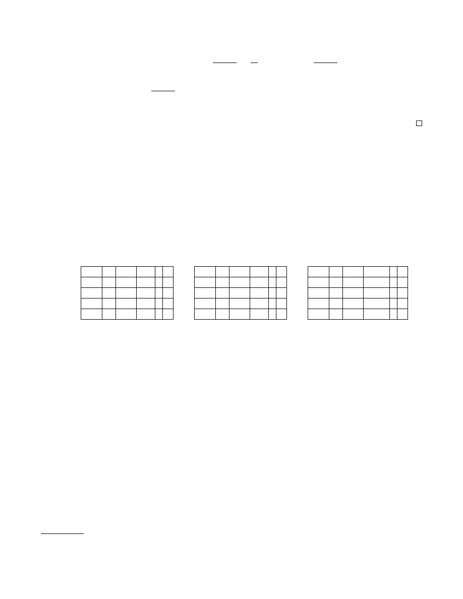
ε
SC
q
w
max
α
β P
2
−128
2
32
1/64 115 4 21
2
−128
2
32
1/16 367 4 23
2
−128
2
32
1/4
1445 4 25
2
−128
2
32
1
6080 4 27
ε
SC
q
w
max
α
β P
2
−192
2
32
1/64 144 4 21
2
−192
2
32
1/16 494 4 23
2
−192
2
32
1/4
2000 4 25
2
−192
2
32
1
8476 4 27
ε
SC
q
w
max
α
β P
2
−256
2
32
1/64 174
4 21
2
−256
2
32
1/16 622
4 23
2
−256
2
32
1/4
2554
4 25
2
−256
2
32
1
10, 871 4 27
5.4
Putting It All Together
Now, we have all the pieces to build an RNG with input that is premature-next robust (by Theorem 2).
Again setting q = 2
32
and assuming w
max
= γ
max
/γ
∗
≈ 32/500 ≈ 1/16, our final scheme can output a
secure 128-bit key in four times the amount of time that it takes to receive roughly 20 to 30 kilobytes of
entropy.
6
Constant-Rate Adversaries
We note that the numbers that we achieve in Section 5.4 are not ideal. But, our security model is also
very strong. So, we follow Ferguson and Schneier [FS03] and consider the weaker model in which the
distribution sampler D is restricted to a constant entropy rate. While this model may be too restrictive, it
leads to interesting results, and it suggests that our construction (or, rather, the slight variant suggested in
Section 6.3) may perform much better against distribution samplers that are not too adversarial. Indeed, if
we think of the distribution sampler D as essentially representing nature, this might not be too unreasonable.
Constant-Rate Model.
We simply modify our definitions in the natural way. First, we say that a
distribution (resp., sequence) sampler is constant if, for all i, γ
i
= γ (resp., w
i
= w) for all i for some
fixed γ (resp., w). Second, we say that an RNG with input is ((t, q
D
, q
R
, q
S
), γ
∗
, γ
max
, ε, β)-premature-next
robust against constant adversaries if it is ((t, q
D
, q
R
, q
S
), γ
∗
, γ
max
, ε, β)-premature-next robust when the
distribution sampler D is required to be constant. Third, we say that a scheduler is (t, q, w
max
, r, ε)-secure
against constant sequences if, for some
α, β such that α · β = r it is (t, q, w
max
, α, β, ε)-secure when the
7
13] contains a detailed discussion of the subtleties here and the justification for such an assumption.
8
We note that when the sequence sampler E must be constant, (t, q, w
max
, α, β, ε)-security is equivalent to (t, q, w
max
, α
0
, β
0
, ε)-
security if α · β = α
0
· β
0
.
16

sequence sampler E is required to be constant. When ε = 0 and the adversaries are allowed unbounded
computation (as is the case in our construction), we simply leave out the parameters t and ε.
Finally, we note that our composition theorem, Theorem 2, applies equally well in the constant-rate
case. In particular, replacing a secure scheduler with a scheduler that is secure against constant sequences
results in an RNG with input that is premature-next robust against constant adversaries, with identical
parameters. This will allow us to achieve much better parameters for schedulers and RNGs with input
against constant adversaries.
6.1
Optimizing Fortuna’s Scheduler
Ferguson and Schneier essentially analyze the security of a scheduler that is a deterministic version of our
scheduler from Section 5.2, with pseudorandom choices replaced by round-robin choices [FS03]. (This is,
of course, where we got the idea for our scheduler.) They conclude that it achieves a competitive ratio of
2 log
2
q. However, the correct value is 3 log
2
q.
Ferguson and Schneier’s model differs from ours in that
they do not consider adversarial starting times τ
0
between the emptying of pools. Taking this (important)
consideration into account, it turns out that SC
F
achieves a competitive ratio of r
F
= 3.5 log
2
q in our
model (e.g., for q = 2
32
, we get r
F
= 112, as opposed to their claimed value of 64).
Interestingly, the pseudocode in [FS03] actually describes a potentially stronger scheduler than the one
that they analyzed. Instead of emptying just pool i, this new scheduler empties each pool j with j ≤ i.
Although Ferguson and Schneier did not make use of this in their analysis, we observe that this would
lead to significantly improved results provided that the scheduler could “get credit” for all the entropy from
multiple pools. Unfortunately, our model syntactically cannot capture the notion of multiple pools being
emptied at once, and this is necessary for our composition theorem (Theorem 2). Fortunately, we notice
that our model can simulate a multiple-pool scheduler by simply treating any set of pools that is emptied
together at a given time as one new pool.
In Appendix B, we make this observation concrete and further optimize the scheduler of Fortuna to
obtain the following result.
Theorem 5. For any integer b ≥ 2, there exists a keyless scheduler SC
b
that is (q, w
max
, r
b
)-secure against
constant sequences where
r
b
=
b +
w
max
b
+
1 − w
max
b
2
· (log
b
q − log
b
log
b
q − log
b
(1/w
max
)) .
In particular, with w
max
= 1 and q → ∞, b = 3 is optimal with r
3
≈ 2.1 log
2
q ≈
r
F
1.66
≈
r
2
1.19
≈
r
4
1.01
.
We note that SC
b
performs even better in the non-asymptotic case. For example, in the case that Ferguson
and Schneier analyzed, q = 2
32
and w
max
= 1, we have r
3
≈ 58.2 ≈
r
F
1.9
, saving almost half the entropy
compared to Fortuna.
6.2
Constant-Rate Instantiation
Using the results from above, we note that applying our generalized Fortuna construction with the scheduler
from Appendix B with b = 3, q = 2
32
, and w
max
= 1 yields an RNG with input that can achieve a secure
128-bit key after accumulating 3 to 4.5 kilobytes of entropy from a constant distribution sampler D. So,
this constant-rate construction (in this restricted setting) is over twenty-five more efficient than our general
construction.
(In Section 6.3, we present a scheduler that achieves these better results in the constant-rate
case but also achieves the results presented in Section 5 in our stronger model.)
9
There is an attack: Let w = 1/(2
i
+ 1) and start Fortuna’s counter so that pool i + 1 is emptied after 2
i
· log
2
q steps. Clearly,
SC
F
takes (2
i
+ 2
i+1
) · log
2
q = 3 · 2
i
· log
2
q total steps to finish, achieving a competitive ratio arbitrarily close to 3 log
2
q.
10
This follows from the analysis of our own scheduler in Appendix B.
11
To compare with our previous numbers from Section 5, recall that we had β = 4. Therefore, we note that the above scheduler
achieves such security in four times the amount of time that it takes to receive about 750 bytes to 1.2 kilobytes of entropy.
These are the proper numbers to compare, though they make less sense in the constant-rate case.
17

Ferguson and Schneier claim in [FS03] that their underlying seed (the key for AES in counter mode)
reaches a secure 128-bit key after receiving what amounts to over 1.7 kilobytes of entropy (after accounting
for the error and difference in models mentioned in Section 6). However, we note that they implicitly assume
that their construction achieves perfect entropy accumulation. We achieve formally provable security and
lose roughly a factor of four from using the construction of [DPR
13] described in Section 5 to accumulate
entropy, though due to various optimizations we manage to come within a factor of about 2 of Ferguson
and Schneier’s claim.
6.3
A Scheduler Secure in Both Worlds
Recall that in Section 5.2, we construct a secure scheduler, and above we construct a keyless scheduler that
is secure only against constant sequence samplers but achieves much better parameters. We justify this
weaker model by arguing that, in practice, a purely adversarial distribution sampler may be too stringent.
We would like to say that the “true” security of our construction in a “real world” setting lies somewhere in
between. And, we would like to say that practitioners can use one scheduler that is provably secure in the
stronger model and achieves excellent parameters when adversaries happen to be friendlier.
However, this is unfortunately not true for the scheduler that we presented in Section 5.2. Recall that
this scheduler selected which pool to fill at a given time pseudorandomly, using a PRF. It is not hard to
see that its performance against constant sequence samplers is only slightly better than its performance
against arbitrary adversaries. Intuitively, our keyless scheduler distributes weight evenly amongst all of its
pools, while our more secure scheduler only does so in expectation. As a result, it can put entropy in the
“wrong pool” with fairly high probability, even in the constant-rate case.
Luckily, there is a fairly simple solution. Instead of selecting a new pool pseudorandomly at each step,
we instead choose a pseudorandom permutation of all P pools every P steps. In particular, given a state τ
and a key skey, the scheduler computes π ← F(skey, bτ /P c) where π is a permutation of P elements, F is a
pseudorandom function whose range is all permutations on P elements, and P is the number of pools of the
scheduler. It then fills pool in ← π(τ mod P ). The scheduler can otherwise behave like our scheduler from
Section 6. It is not hard to see that our proofs of security in both the constant-rate and general case apply
immediately to this modified scheduler. So, we recommend that practitioners implement this construction.
7
Relaxing the Seed Independence of the Distribution Sampler
In this section, we address another limitation of the original model of [DPR
13], which our model inherits:
the subtle issue of seed independence. In particular, the model of [DPR
13] does not allow the distribution
sampler D to have access to the initial seed seed of the RNG with input.
As explained by [DPR
13], this is necessary to some extent, as there is a very simple impossibility
result when D knows the seed. Given any RNG with input G whose input length is p ≥ 2, consider
D that simply samples I
1
, . . . , I
q
D
uniformly such that next(seed, S
q
D
) starts with a 0 where S
0
= 0, and
S
j
= refresh(seed, S
j−1
, I
j
). Let A be the adversary that simply calls set-state(0), makes q
D
calls to D-refresh,
calls next-ror, and simply outputs the first bit of the resulting output. It is clear that this pair of A and D
will break the RNG security, and also that H
∞
(I
j
|I
1
, . . . , I
j−1
, I
j+1
, . . . I
q
D
) ≈ p − 1.
In fact, the original provably secure scheme from [DPR
13] can be attacked much more dramatically
(than the above generic attack) by a seed-dependent D. Recall, in that scheme part of the seed X, input
I, and state S are simply elements in a finite field F
2
n
. Also, if the start state S is 0 and the distribution
sampler D samples some random variables I
1
, . . . , I
q
D
, then after q
D
refresh calls the resulting state will be
S = X
q
D
−1
I
1
+ X
q
D
−2
I
2
+ . . . + I
q
D
. This suggests a natural attack: simply let I
j
be sampled uniformly
from {0, X
j−q
D
}. Clearly the distribution sampler provides q
D
bits of entropy in this case, but a quick
check shows that the state S is the sum of uniformly random bits, so it can be only 0 or 1. The distribution
sampler can therefore provide arbitrarily large amounts of entropy while only letting the state accumulate
one bit.
18

Unfortunately, our generalized Fortuna scheme that is premature-next robust suffers a similar fate, even
without attacking any of the “pool” RNGs. Indeed, if the distribution sampler D has access to the seed, then
in particular, it has access to the key skey of the scheduler. D can therefore choose to only provide entropy
to pools that will soon be emptied. For example, against our scheduler in Section 5.2, D can provide 1 bit of
entropy whenever pool 0 will be filled next, and no entropy otherwise. If the adversary A then calls get-next
repeatedly after every D-refresh call, the RNG will never accumulate any entropy (with high probability).
To sum up, existing schemes crucially rely on the seed-independence of the distribution sampler, and it
is also clear that full seed-dependence is impossible. Finding the right (realistic and, yet, provably secure)
balance between these extremes is an important subject for further research. In the next subsection, we
make some initial progress along these lines by introducing a somewhat realistic model that effectively
allows a certain level of seed dependence.
7.1
Semi-Adaptive set-refresh
Our extended adversarial model is motivated by the following realistic scenario given by Ferguson and
Schneier when describing Fortuna [FS03]. They assume that there are several sources of entropy N
1
, N
2
, . . .
contributing the inputs I
j
for the D-refresh procedure. Some of these sources might be completely controlled
by the attacker A, while others are assumed to provide “good” entropy. Of course, since the actual RNG
does not know the identity of these adversarial sources, they suggest that the RNG should take the inputs
from N
1
, N
2
, . . . in a round-robin manner, ensuring that “good” sources periodically contribute fresh entropy
to the system.
Semi-Adaptive set-refresh Model. Translating this natural attack scenario to our model (for both ROB
and NROB), we can think of the union of “good” sources N
i
as our original (seed-independent) distribution
sampler D, while the union of “bad” source N
i
can be modeled by giving the (seed-dependent) attacker A
access to the simple set-refresh oracle shown in Figure 9.
proc. set-refresh(I
∗
)
S ← refresh(S, I
∗
)
Fig. 9: The set-refresh oracle
Note, in particular, that since set-refresh is called by A, the entropy counter
c is not incremented during this call. Additionally, since in the above moti-
vating example the RNG will call the good/bad entropy sources in a round-
robin manner, it seems reasonable to make the assumption that the order of
set-refresh calls is seed-independent (though, crucially, the values I
∗
in various
set-refresh(I
∗
) calls can depend on the seed).
Overall, we can think of A and
D as defining a partially seed-dependent distribution sampler D
0
.
We arrive at the following natural extension of robustness, which we call the semi-adaptive set-refresh
model, where q
D
is now the maximal sum of the number D-refresh and the set-refresh calls made by A:
– D selects a subset of indices J ⊆ {1, . . . , q
D
} where set-refresh calls will be made.
– A learns seed and J , and can play the usual ROB/NROB game, except the sequence of its D-refresh and
set-refresh calls must be consistent with J . I.e., the j-th such call must be set-refresh iff j ∈ J .
Security Against Semi-adaptive set-refresh. We observe that the robustness proofs of both the original
RNG construction of [DPR
13] and our generalized Fortuna construction easily extend to handle semi-
adaptive set-refresh calls. Indeed, we even achieve identical parameters.
Interestingly, we are not aware of an attack on [DPR
13]’s construction even with seed-dependent (i.e.,
fully-adaptive) set-refresh calls, but our current proof crucially uses semi-adaptivity. Unfortunately, our
attack on generalized Fortuna with a seed-dependent distribution sampler easily extends to an attack using
seed-dependent (i.e., fully-adaptive) set-refresh calls instead. Indeed, using skey, A can schedule set-refresh
calls such that D-refresh calls only affect pools that will soon be emptied.
12
Note that, while this assumption is quite strong, we do not impose a fixed order on the set-refresh calls or assume constant
entropy from D-refresh calls as [FS03] do. Indeed, the original Fortuna construction is clearly not secure in our extended
model even with a constant entropy assumption.
19

Theorem 6. The security bound for the RNG of [DPR
13] given in Theorem 3 extends to the semi-
adaptive set-refresh model. Similarly, the premature next robustness of the generalized Fortuna scheme given
in Theorem 2 extends to the semi-adaptive set-refresh model, provided all the pool RNGs G
i
are robust in
the semi-adaptive set-refresh model.
Since both proofs are simple variants of the original proofs, we will only sketch the key steps required
to extend both proofs below.
Extending the Composition Theorem. We first show how to extend the proof of our main composition
theorem (Theorem 2) to handle semi-adaptive set-refresh. To do so, we need to show how to extend the
main reduction, mapping the “big” attackers A, D against the composed RNG G into “small” attackers A
i
, D
i
against the pool RNG G
i
, to the semi-adaptive set-refresh setting. Fortunately, this is simple because the
scheduler key skey in our reduction is selected directly by D
i
(see Figure 6) and then immediately passed
to A
i
via leakage. In particular, D
i
can now also compute the index set J , then use skey to “project” this
set J to whatever calls j ∈ J will be “routed” to G
i
by the scheduler, and finally pass this “projected set”
J
i
to the challenger. A
i
then learns the seed and J
i
and can simulate the run of A as before (see Figure 7),
handling set-refresh calls in the obvious way.
Extending [DPR
13]’s Proof.
Next, we sketch the changes needed to extend the original proof of
robustness of the [DPR
13] construction (see Section 5.1) to handle semi-adaptive set-refresh calls. The proof
of [DPR
13] consists of three steps: (1) reducing robustness to two simpler properties called preserving and
recovering security (see [DPR
13]’s Theorem 1); (2) showing preserving security; and (3) showing recovering
security. Step (1) easily extends to semi-adaptive set-refresh calls, provided the notion of recovering security
is naturally augmented to include semi-adaptive set-refresh calls. Step (2) needs no changing at all (as
preserving security already gives A access to a fully adaptive set-refresh oracle). Hence, it suffices to show
how to extend the proof of recovering security in step (3) to a slightly modified version that includes
set-refresh calls. We present the modified recovery security game together with the preserving security game
and a modified version of [DPR
13]’s composition theorem in Appendix C.
Intuitively, recovering security considers an attacker that sets the state to some arbitrary value S
0
and
starts the distribution sampler D after k calls to D-refresh. Following that, d calls to D-refresh are made,
resulting in final state S, where d, k are chosen by A such that the corrupt flag is false after the d calls to
D-refresh. Then, the attacker A attempts to distinguish the full output (S
∗
, R) ← next(S) from uniform. In
our modified version, an index set J is chosen by D at the beginning, and the j-th D-refresh call is replaced
by a set-refresh call if and only if j ∈ J .
Note that in the recovering game, [DPR
13]’s RNG with input effectively computes a function of the
form
h
∗
X,X
0
(I
1
, . . . , I
d
) =
h
X
0
·
d−1
X
j=0
I
d−j
· X
j
i
m
1
+ [X
0
· S
0
]
m
1
and applies a PRG G to the result. In [DPR
13], the authors show that recovering security follows imme-
diately from the fact that h
∗
X,X
0
is a good randomness extractor. In particular, if the sum of the conditional
min-entropies of the input is sufficiently high (i.e., above γ
∗
) and the I
j
are chosen independently of X, X
0
,
then (X, X
0
, h
∗
X,X
0
(I
1
, . . . , I
D
)) is ε
ext
-close to uniform (with ε
ext
defined as in Theorem 3).
Our key observation is simply that h
∗
X,X
0
is linear. Intuitively, we wish to define three sequences:
I
D,A
j
(seed) is the sequence of inputs to refresh calls, including both D-refresh and set-refresh; I
D
j
is the
contribution from D-refresh calls; and I
A
j
(seed) is the contribution from A’s set-refresh calls. We then want
to say that h
∗
X,X
0
applied to I
D,A
j
is the sum of h
∗
X,X
0
applied to each adversary’s contribution.
In particular, fix A, D. Let (I
j
)
q
D
j=1
be the distributions sampled by D; J the index set chosen by D,
seed = (X, X
0
) a randomly chosen seed; k, d the (seed-dependent) choices of A; and (I
∗
j
(seed))
j∈J
the input
of A to set-refresh calls. Then, formally, we let I
D
j
= I
D,A
j
(seed) = I
j
and I
A
j
(seed) = 0 if j /
∈ j, and
20

I
A
j
(seed) = I
D,A
j
(seed) = I
∗
j
(seed) and I
D
j
= 0 if j ∈ J . We can then write
U := h
∗
X,X
0
I
A,D
k+1
(seed), . . . , I
A,D
k+d
(seed)
+ [X
0
· S
0
]
m
1
= h
∗
X,X
0
I
D
k+1
, . . . , I
D
k+d
+ h
∗
X,X
0
I
A
k+1
(seed), . . . , I
A
k+d
(seed)
+ [X
0
· S
0
]
m
1
.
Finally, we simply note that I
D
j
are chosen independently from X, X
0
(equivalently, they are the output of
some valid distribution sampler D
0
), and therefore the proof of [DPR
13] implies that (X, X
0
, h
∗
X,X
0
(I
D
k+1
, . . . , I
D
k+d
))
is ε
ext
close to uniform when the sum of the entropies of the corresponding distributions is sufficiently high.
This of course immediately implies that X, X
0
, U is also ε
ext
close to uniform. The result, presented below,
then follows immediately from the proof in [DPR
Theorem 7. Let n > m, `, γ
∗
be integers and ε
ext
∈ (0, 1) such that γ
∗
≥ m + 2 log(1/ε
ext
) + 1 and n ≥
m+2 log(1/ε
ext
)+log(q
D
)+1. Assume that G : {0, 1}
m
→ {0, 1}
n+`
is a deterministic (t, ε
prg
)-pseudorandom
generator. Let G = (setup, refresh, next) be defined as in Section 5. Then G is a ((t
0
, q
D
, q
R
, q
S
), γ
∗
, ε)-robust
RNG with input in the semi-adaptive set-refresh model where t
0
≈ t, ε = q
R
(2ε
prg
+ q
2
D
ε
ext
+ 2
−n+1
).
Combining Theorems 6 and 7, we see that the security of the instantiation that we presented in Section 5
immediately extends to the semi-adaptive set-refresh model with identical parameters.
References
BH05.
Boaz Barak and Shai Halevi. A model and architecture for pseudo-random generation with applications to /de-
v/random. In Proceedings of the 12th ACM Conference on Computer and Communications Security, CCS ’05,
pages 203–212, New York, NY, USA, 2005. ACM.
BK12.
Elaine Barker and John Kelsey. Recommendation for random number generation using deterministic random bit
generators. NIST Special Publication 800-90A, 2012.
BR06.
Mihir Bellare and Phillip Rogaway. The security of triple encryption and a framework for code-based game-playing
proofs. In Serge Vaudenay, editor, Advances in Cryptology - EUROCRYPT 2006, volume 4004 of Lecture Notes in
Computer Science, pages 409–426. Springer Berlin Heidelberg, 2006.
CVE08.
CVE-2008-0166. Common Vulnerabilities and Exposures, 2008.
DGP07.
Leo Dorrendorf, Zvi Gutterman, and Benny Pinkas. Cryptanalysis of the random number generator of the windows
operating system. IACR Cryptology ePrint Archive, 2007:419, 2007.
DPR
+
13.
Yevgeniy Dodis, David Pointcheval, Sylvain Ruhault, Damien Vergniaud, and Daniel Wichs. Security analysis
of pseudo-random number generators with input: /dev/random is not robust. In Proceedings of the 2013 ACM
SIGSAC Conference on Computer Communications Security, CCS ’13, pages 647–658, New York, NY, USA, 2013.
ACM.
ESC05.
D. Eastlake, J. Schiller, and S. Crocker. RFC 4086 - Randomness Requirements for Security, June 2005.
Fer13.
Niels Ferguson. Private communication, 2013.
FS03.
Niels Ferguson and Bruce Schneier. Practical Cryptography. John Wiley & Sons, Inc., New York, NY, USA, 1
edition, 2003.
GPR06.
Zvi Gutterman, Benny Pinkas, and Tzachy Reinman. Analysis of the linux random number generator. In Proceed-
ings of the 2006 IEEE Symposium on Security and Privacy, SP ’06, pages 371–385, Washington, DC, USA, 2006.
IEEE Computer Society.
HDWH12. Nadia Heninger, Zakir Durumeric, Eric Wustrow, and J. Alex Halderman. Mining your Ps and Qs: Detection of
widespread weak keys in network devices. In Proceedings of the 21st USENIX Security Symposium, August 2012.
ISO11.
Information technology - Security techniques - Random bit generation. ISO/IEC18031:2011, 2011.
Kil11.
Killmann, W. and Schindler, W. A proposal for: Functionality classes for random number generators. AIS 20 /
AIS31, 2011.
KSF99.
John Kelsey, Bruce Schneier, and Niels Ferguson. Yarrow-160: Notes on the design and analysis of the yarrow
cryptographic pseudorandom number generator. In In Sixth Annual Workshop on Selected Areas in Cryptography,
pages 13–33. Springer, 1999.
KSWH98. John Kelsey, Bruce Schneier, David Wagner, and Chris Hall. Cryptanalytic attacks on pseudorandom number
generators. In Serge Vaudenay, editor, Fast Software Encryption, volume 1372 of Lecture Notes in Computer
Science, pages 168–188. Springer Berlin Heidelberg, 1998.
LHA
+
12.
Arjen K. Lenstra, James P. Hughes, Maxime Augier, Joppe W. Bos, Thorsten Kleinjung, and Christophe Wachter.
Public keys. pages 626–642, 2012.
LRSV12.
Patrick Lacharme, Andrea Röck, Vincent Strubel, and Marion Videau. The linux pseudorandom number generator
revisited. IACR Cryptology ePrint Archive, 2012:251, 2012.
21

NS02.
Nguyen and Shparlinski. The insecurity of the digital signature algorithm with partially known nonces. Journal
of Cryptology, 15(3):151–176, 2002.
SV03.
Amit Sahai and Salil P. Vadhan. A complete problem for statistical zero knowledge. J. ACM, 50(2):196–249, 2003.
Wik04.
Wikipedia. /dev/random. http://en.wikipedia.org/wiki//dev/random, 2004. [Online; accessed 09-February-
2014].
A
Proof of Theorem 1
We prove the two bounds in Theorem 1 as two separate propositions. Note that the first lower bound applies
even when adversaries are restricted to just constant sequences.
Proposition 1. For q ≥ 3, let SC be a (t, q, w
max
, α, β, ε)-secure scheduler against constant-rate adversaries
running in time t
SC
. Then, either t = O(q · (t
SC
+ log q)), ε ≥ 1/(q − 1/w
max
+ 1), or
r > log
e
q − log
e
(1/w
max
) − log
e
log
e
q − 1 ,
where r = α · β is the competitive ratio.
Proposition 2. Suppose that SC is a (t, q, w
max
, α, β, ε)-secure scheduler running in time t
SC
. Then, either
t = O(q(t
SC
+ log q)), r
2
> w
2
max
q, ε ≥ 1/e, or
α >
w
max
w
max
+ 1
·
log
e
(1/ε) − 1
log
e
log
e
(1/ε) + 1
,
where r = α · β.
It should be clear that Theorem 1 follows immediately from the two propositions.
A.1
Proof of Proposition 1
The main step in the proof of Proposition 1 is the following lemma:
Lemma 1. For any q ≥ 3 let E
i
be the constant sequence sampler that simply outputs the sequence
(1/i, . . . , 1/i) for i = 1/w
max
, . . . q. Then, for any keyless scheduler SC with P pools, there exists an i and an
adversary A such that E
i
and A win SGAME(P, q, w
max
, r) for any r > log
e
q −log
e
(1/w
max
)−log
e
log
e
q −1.
Furthermore, there exists a single adversary A
0
that, given any keyless scheduler SC, i, and r, can
output the τ that allows E
i
to win SGAME(P, q, w
max
, r) against SC (or outputs FAIL if none exists) in time
O(q · (log q + t
SC
)), where t
SC
is the run-time of the scheduler.
Proof. We assume without loss of generality that 1/w
max
is an integer.
Fix any keyless scheduler SC and start state τ
0
. Given the corresponding sequence (in
j
, out
j
)
q
j=1
, we
define the sequence of “leave times” b
1
, . . . b
q
∈ N ∪ {∞} as b
j
= min{T ≥ j : out
T
= in
j
} (where we adopt
the convention that min ∅ = ∞). Intuitively, at time T , we imagine the scheduler selecting a pool in
T
in
which to “throw a ball”, and a pool out
T
to empty afterwards. The leave time b
j
is the time at which the
ball that was “thrown” at time j will “leave the game”.
Let τ
T
be the state of SC after T steps, and let A
T
be the adversary that sets the state of SC to τ
T
. Note
that SC wins SGAME(P, q, w
max
, r) against E
i
, A
T
if and only if there is some set of i balls J ⊆ [T +1, T +i·r]
with b
j
= b
j
0
≤ T + i · r for all j, j
0
∈ J .
We proceed by “marking balls”. We first consider b
w
max
·q
r
c non-overlapping intervals of length r/w
max
in {1, . . . , q}. By hypothesis, there must be at least 1/w
max
balls in each of these intervals that leave at the
same time in the same interval. We mark all such balls, marking at least
q
r
− 1/w
max
distinct balls in total.
Now, consider b
w
max
·q
2r
c non-overlapping intervals of length 2r/w
max
. In each such interval, there must be
at least 2/w
max
balls whose leave time is the same and in the interval. We mark these balls. Previously
no more than 1/w
max
balls that we’d marked had the same leave time, so we must have marked at least
22

1/w
max
new balls in each interval. Therefore, we’ve now marked at least
q
r
+
q
2r
− 2/w
max
distinct balls, and
no set of more than 2/w
max
balls have the same leave time.
Proceeding by induction, suppose that after j < b
w
max
·q
r
c steps, we have marked at least
P
j
k=1
q
k·r
−
j/w
max
distinct balls, and no set of more than j/w
max
marked balls have the same leave time. We consider
b
w
max
·q
(j+1)·r
c non-overlapping intervals of length (j + 1) · r/w
max
and note that in each such interval there must
be (j + 1)/w
max
balls with the same leave time. So, we mark these and note that we must have marked an
additional
q
2r
− 1/w
max
new balls and that no set of more than (j + 1)/w
max
marked balls have the same
leave time.
It follows that this procedure will mark at least
P
bw
max
·q/rc
k=1
q
k·r
− q/r balls. Recalling that the nth
harmonic number satisfies H
n
=
P
n
k=1
1/k > log
e
(n + 1), it follows that we’ve marked at least
q
r
· (log
e
q −
log
e
r − log
e
(1/w
max
) − 1) distinct balls in this way. But, there are only q balls total. It follows that
r > log
e
q − log
e
(1/w
max
) − log
e
log
e
q − 1.
It remains to construct an A
0
that finds the winning τ in O(q · (t
SC
+ log q)) time given SC, i, and r.
A
0
first computes (τ
j
)
q−1
j=0
in time O(q · t
SC
). Now, as above, A
0
divides {1, . . . , q} into disjoint intervals of
length b
q
i·r
c. For each such interval [T + 1, T + i · r], A
0
simply simulates SGAME(P, i · r, r) against E
i
starting
at τ
T
A returns τ
T
if it wins the simulation. If no τ
T
wins, A
0
outputs FAIL. This takes time O(q log q).
(The log q overhead is incurred because A needs to write numbers that could be as large as q.)
The result follows.
From this, Proposition 1 follows easily.
Proof of Proposition 1. Fix SC.
Let E be the sequence sampler that selects i
$
← {1/w
max
, . . . , q} and then behaves as the constant
sequence sampler E
i
from Lemma 1. Let A be the adversary that behaves as follows: On input skey, A
produces the keyless scheduler SC
skey
such that SC
skey
(σ) = SC(skey, σ). A then simulates A
0
from the
lemma, which outputs either some state τ or FAIL. If A
0
outputs τ , A simply does the same. Otherwise, A
outputs an arbitrary state.
By Lemma 1, A runs in time O(q·(log q+t
SC
)), and if r ≤ log
e
q−log
e
(1/w
max
)−log
e
log
e
q−1, then with
probability at least 1/(q −1/w
max
+1), this procedure produces an E
i
, τ pair that wins SGAME(P, q, w
max
, r)
against SC
skey
. The result follows.
A.2
Proof of Proposition 2
Proof of Proposition 2. Suppose r
2
≤ w
2
max
q. For simplicity, we will assume 1/w
max
is an integer.
Our proof begins similarly to that of Lemma 1. In particular, we let τ
0
be any start state. Let B
1
, . . . , B
q
be random variables over the choice of skey corresponding to leave times, B
j
= min{T ≥ j : out
T
= in
j
}.
We again think of a ball with weight w
j
thrown into pool in
j
at time j and leaving the game at time B
j
.
Intuitively, our approach will be to first show a pair of adversaries that win if balls take too long to
leave. We’ll then show a pair of adversaries that win if balls leave too quickly.
In particular, let E simply output a sequence of α/w
max
maximum weights followed by 0s, (w
max
, . . . , w
max
, 0, . . . 0).
For any skey and any 1 ≤ T ≤ q, let τ
T
(skey) be the state that SC with skey reaches after T steps,
starting at τ
0
. Let A
k
be the adversary that simply outputs τ
kr/w
max
(skey) on input skey. Note in or-
der for SC to win SGAME against E , A
k
, it is necessary but not sufficient for there to be some j with
kr/w
max
< j ≤ kr/w
max
+ α/w
max
and B
j
≤ (k + 1)r/w
max
. (Intuitively, there must be some ball that
enters in the first α/w
max
steps of the game against A
k
and leaves before time r/w
max
.)
Now, let A
∗
k
be an adversary that for 0 ≤ k
0
< k selects j
k
0
uniformly at random with k
0
r/w
max
< j
k
0
≤
k
0
r/w
max
+ α/w
max
. If B
j
k0
> (k
0
+ 1) · r/w
max
, then A
∗
k
simply behaves as A
k
0
. Otherwise, A
∗
k
behaves as
A
k
. Let E
k
be the event that B
j
k0
< (k
0
+ 1) · r/w
max
for all k
0
≤ k. Note that A
∗
k
wins if E
k
happens and
13
Technically, we replace E
i
with E
0
i
, which outputs a sequence of length i · r.
23
B
j
> (k + 1) · r/w
max
for all j with kr/w
max
< j ≤ kr/w
max
+ α/w
max
. (To be clear, A
∗
k
may win in other
circumstances as well.) Therefore,
ε ≥ Pr[E
k
] · Pr
h
∀j with
kr
w
max
< j ≤
kr + α
w
max
, B
j
> (k + 1) ·
r
w
max
E
k
i
.
Rearranging, we have
Pr[E
k
] − ε ≤ Pr[E
k
] · Pr
h
∃j with
kr
w
max
< j ≤
kr + α
w
max
, B
j
≤ (k + 1) ·
r
w
max
E
k
i
≤ Pr[E
k
] ·
(k·r+α)/w
max
X
j=k·r/w
max
Pr
h
B
j
≤ (k + 1) ·
r
w
max
E
k
i
=
α
w
max
· Pr[E
k
] · Pr
h
B
j
k
≤ (k + 1) ·
r
w
max
E
k
i
=
α
w
max
· Pr[E
k+1
] ,
where B
j
k
is chosen uniformly at random with kr/w
max
< j
k
≤ kr/w
max
+ α/w
max
. So, we have the
recurrence relation Pr[E
k
] ≥ (w
max
/α) · (Pr[E
k−1
] − ε), with Pr[E
0
] = 1. It follows that
Pr[E
k
] ≥
w
max
α
k
− ε ·
k
X
i=1
w
max
α
i
>
w
max
α
k
− ε ·
w
max
α − w
max
.
Now, let E
∗
be the sequence sampler that randomly selects j
k
with kr/w
max
< j
k
≤ kr/w
max
+ α/w
max
for all k < (w
max
+ 1) · α/w
max
. E
∗
then outputs the sequence (w
i
) where w
i
= w
max
/(w
max
+ 1) if i = j
k
for some k and w
i
= 0 otherwise. Suppose the event E
k
∗
occurs where k
∗
= (w
max
+ 1) · (α − 1)/w
max
+ 1.
Then, for all k ≤ k
∗
, the j
k
-th ball leaves before the j
k+1
-st ball enters. In particular, E
∗
, A
0
win SGAME.
Therefore,
ε ≥ Pr[E
k
∗
] >
w
max
α
k
∗
− ε ·
w
max
α − w
max
.
It follows that
α >
w
max
w
max
+ 1
·
log
e
(1/ε) − 1
log
e
log
e
(1/ε) + 1
provided that ε < 1/e.
It is easy to see that A
∗
k
and E
∗
run in time O(q(t
SC
+ log q)), and the result follows.
B
Construction of Constant-Rate Scheduler and Proof of Theorem 5
We first notice that Fortuna’s scheduler can be easily modified to use a different base. In particular, for
any integer b ≥ 2, we define a keyless scheduler, SC
b
. Roughly, SC
b
has P
b
≈ log
b
q pools, numbered
0, . . . , P
b
− 1. The state τ ∈ {0, . . . , q − 1} will just be a counter. The pools are filled in turn, and pool i is
emptied whenever the counter τ divides b
i
· P
b
but not b
i+1
· P
b
.
Our actual construction will be slightly more involved than the above, but it is simply an optimized
version of this basic idea. In particular, we make four changes:
1. We account for w
max
by emptying pools when τ divides b
i
· P
b
/w
max
, instead of just b
i
· P
b
.
2. We use slightly fewer than log
b
q pools, setting P
b
= log
b
q − log
b
log
b
q − log
b
(1/w
max
).
3. We do not empty the 0th pool twice in a row. (While this never comes up when b = 2, it is an issue for
b ≥ 3.)
4. If pool j will next be emptied sooner than pool i and j > i, we fill pool j instead of pool i. (This
captures the idea of emptying multiple pools at once from Section 6.)
24
proc. SC
b
(τ ) :
IF τ 6= 0 mod P
b
/w
max
, THEN out ← ⊥
ELSE
j ← max{j : τ = 0 mod b
j
· P
b
/w
max
}
IF j = 0 AND τ − P
b
/w
max
6= 0 mod b · P
b
/w
max
out ← ⊥
// Don’t empty pool 0 twice in a row
ELSE out ← j
i ← τ − 1 mod P
b
// Find the next time τ
∗
that a pool with index at least i will be emptied
τ
∗
← min{τ
∗
≥ τ : τ
∗
= 0 mod b
i
· P
b
/w
max
}
// Fill the pool emptied at time τ
∗
in ← max{in : τ
∗
= 0 mod b
in
· P
b
/w
max
}
τ
0
← τ + 1 mod q
OUTPUT (τ
0
, in, out)
Fig. 10: Our keyless scheduler construction
For simplicity, we assume that log
b
log
b
q and log
b
(1/w
max
) are both integers, and we let P
b
= log
b
q −
log
b
log
b
q − log
b
(1/w
max
). Then, we define SC
b
as in Figure 10.
Theorem 5 shows that this scheme achieves a very good competitive ratio of r
b
≈ bP
b
. In Appendix A,
we show a lower bound in the constant-rate case of r > log
e
q − log
e
log
e
q − log
e
(1/w
max
) − 1 (or r > P
e
− 1
in slightly abused notation), so this result is very close to optimal.
Proof of Theorem 5. Note that E must output a constant sequence, (w, . . . , w) with r
b
/q ≤ w ≤ w
max
. (If
w < r
b
/q, then we win by default.) We assume without loss of generality that 1/w is an integer.
We first handle the case when w > w
max
/b. Note that no pool is emptied more than once every
b
w
max
· P
b
steps and at least one pool is emptied every
b−1
w
max
· P
b
steps. So, if w > w
max
/b, SC
b
wins as soon as the
first pool is emptied after
1
w
· P
b
steps, in time at most (
1
w
+
b−1
w
max
) · P
b
. It therefore achieves a competitive
ratio of less than (1 + (b − 1) ·
w
w
max
) · P
b
≤ bP
b
.
Now, assume w ≤ w
max
/b.
Let i ≥ 1 such that
b
i+1
−1
b−1
≥ w
max
/w >
b
i
−1
b−1
. Consider the first time a pool whose index is at least i
is emptied. If it is full on this first emptying, then SC
b
wins, in time at most b
i
· P
b
/w
max
. Otherwise, let
T
∗
be the first time such a pool is emptied. Then, SC
b
wins the next time a pool whose index is greater
than i is emptied, at time T
∗
+ b
i
· P
b
/w
max
. In both cases, SC
b
achieves a competitive ratio of at worst
r
b
= w · (T
∗
+ b
i
· P
b
/w
max
).
We wish to bound T
∗
. Let j such that b
j+1
> w
max
· T
∗
/P
b
≥ b
j
. Then, at time T
∗
the pool that is
emptied has weight at least
w · bT
∗
/P
b
c +
w
w
max
·
j
X
k=0
b
k
> w ·
T
∗
P
b
+
1
w
max
·
b
j+1
− 1
b − 1
− 1
> w ·
T
∗
P
b
+
1
w
max
·
w
max
·
T
∗
P
b
− 1
b − 1
− 1
=
w · T
∗
P
b
·
b
b − 1
− w ·
1 + (b − 1) · w
max
(b − 1) · w
max
.
Note that the above weight is less than one by hypothesis. Applying this and rearranging,
w · T
∗
<
w + (1 + w)(b − 1) · w
max
b · w
max
· P
b
.
25
Plugging in and recalling that w ≤ w
max
/b and w
max
/w >
b
i
−1
b−1
,
r
b
<
w + (1 + w)(b − 1) · w
max
b · w
max
· P
b
+
w
w
max
·
(b − 1) ·
w
max
w
+ 1
· P
b
≤
(1 + w
max
/b)(b − 1)
b
+
1
b
2
· P
b
+
b − 1 +
1
b
· P
b
=
b +
w
max
b
+
1 − w
max
b
2
· P
b
The result follows.
C
Recovering and Preserving Secutity
C.1
Recovering Security
We consider the following security game with an attacker A, a sampler D, and bounds q
D
, γ
∗
.
– D sends J ⊂ {1, . . . , q
D
} to the challenger.
– The challenge chooses a seed seed
$
← setup, and a bit b
$
← {0, 1} uniformly at random. It sets σ
0
:= 0.
For k = 1, . . . , q
D
, the challenger computes
(σ
k
, I
k
, γ
k
, z
k
) ← D(σ
k−1
).
– The attacker A gets seed, J , and γ
1
, . . . , γ
q
D
, z
1
, . . . z
q
D
. It gets access to an oracle get-refresh() which
initially sets k := 0 on each invocation increments k := k + 1 and outputs I
k
. At some point the attacker
A outputs a value S
0
∈ {0, 1}
n
, an integer d, and I
∗
j
for j ∈ J such that k + d ≤ q
D
and
X
k<j≤k+d
j /
∈J
γ
j
≥ γ
∗
.
– For j = k + 1, . . . , k + d, the challenger computes
S
j
←
refresh(S
j−1
, I
j
) : j /
∈ J
refresh(S
j−1
, I
∗
j
) : j ∈ J
.
If b = 0 it sets (S
∗
, R) ← next(S
d
) and if b = 1 is sets (S
∗
, R) ← {0, 1}
n+`
uniformly at random. The
challenger gives I
k+d+1
, . . . , I
q
D
, and (S
∗
, R) to A.
– The attacker A outputs a bit b
∗
.
Definition 6 (Recovering Security). We say that PRNG with input has (t, q
D
, γ
∗
, ε)-recovering security
if for any attacker A and legitimate sampler D, both running in time t, the advantage of the above game
with parameters q
D
, γ
∗
is at most ε.
C.2
Preserving Security
We define preserving security exactly as in [DPR
13]. Intuitively, it says that if the state S
0
starts uniformly
random and uncompromised and is then refreshed with arbitrary (adversarial) samples I
1
, . . . , I
d
resulting
in some final state S
d
, then the output (S
∗
, R) ← next(S
d
) looks indistinguishable from uniform.
– The challenger chooses an initial state S
0
← {0, 1}
n
, a seed seed ← setup, and a bit b ← {0, 1} uniformly
at random.
26

– The attacker A gets seed and specifies an arbitrarily long sequence of values I
1
, . . . , I
d
with I
j
∈ {0, 1}
n
for all j ∈ [d].
– The challenger sequentially computes
S
j
= refresh(S
j−1
, I
j
, seed)
for j = 1, . . . , d. If b = 0 the attacker is given (S
∗
, R) = next(S
d
) and if b = 1 the attacker is given
(S
∗
, R) ← {0, 1}
n+`
.
– The attacker outputs a bit b
∗
.
Definition 7 (Preserving Security). A PRNG with input has (t, ε)-preserving security if for any at-
tacker A running in time t, the advantage of A in the above game is at most ε.
C.3
Modified Composition Theorem
With these modified definitions, [DPR
13]’s proof of their composition theorem immediately extends to
handle semi-adaptive set-refresh queries.
Theorem 8. Assume that a PRNG with input has both (t, ε
p
)-preserving security and (t, q
D
, γ
∗
, ε
r
)-recovering
security as defined above. Then, it is ((t
0
, q
D
, q
R
, q
S
), γ
∗
, q
R
(ε
r
+ ε
p
))-robust in the semi-adaptive set-refresh
model where t
0
≈ t.
27
Document Outline
- How to Eat Your Entropy and Have it Too — Optimal Recovery Strategies for Compromised RNGs
- Yevgeniy Dodis, Adi Shamir, Noah Stephens-Davidowitz, and Daniel Wichs
Wyszukiwarka
Podobne podstrony:
No You Cant Have It All
Britney Spears When Your Eyes Say It
Why Women Still Can t Have It All
Britney Spears When Your Eyes Say It
200 Ways To Recover Revive Your Hard Drive
Have me on your mind
Is it Glorious to Die for your Country
101 Ways to Fill Your Practice and Keep It Full(1)
comb your hair and curl it
U2 Sometimes You Cant Make It On Your Own
Roxette It Must Have Been Love
It must have been love
chinesepod does it have bones
It could have been
Gary Vaynerchuk Crush It! Why NOW Is the Time to Cash In on Your Passion
Yiruma It s your day
więcej podobnych podstron