92
6 The NOE Effect
© Gerd Gemmecker, 1999
Nuclear O
VERHAUSER
Effect (NOE): resonance line intensity changes caused by dipolare cross-
relaxation from neighbouring spins with perturbed energy level populations.
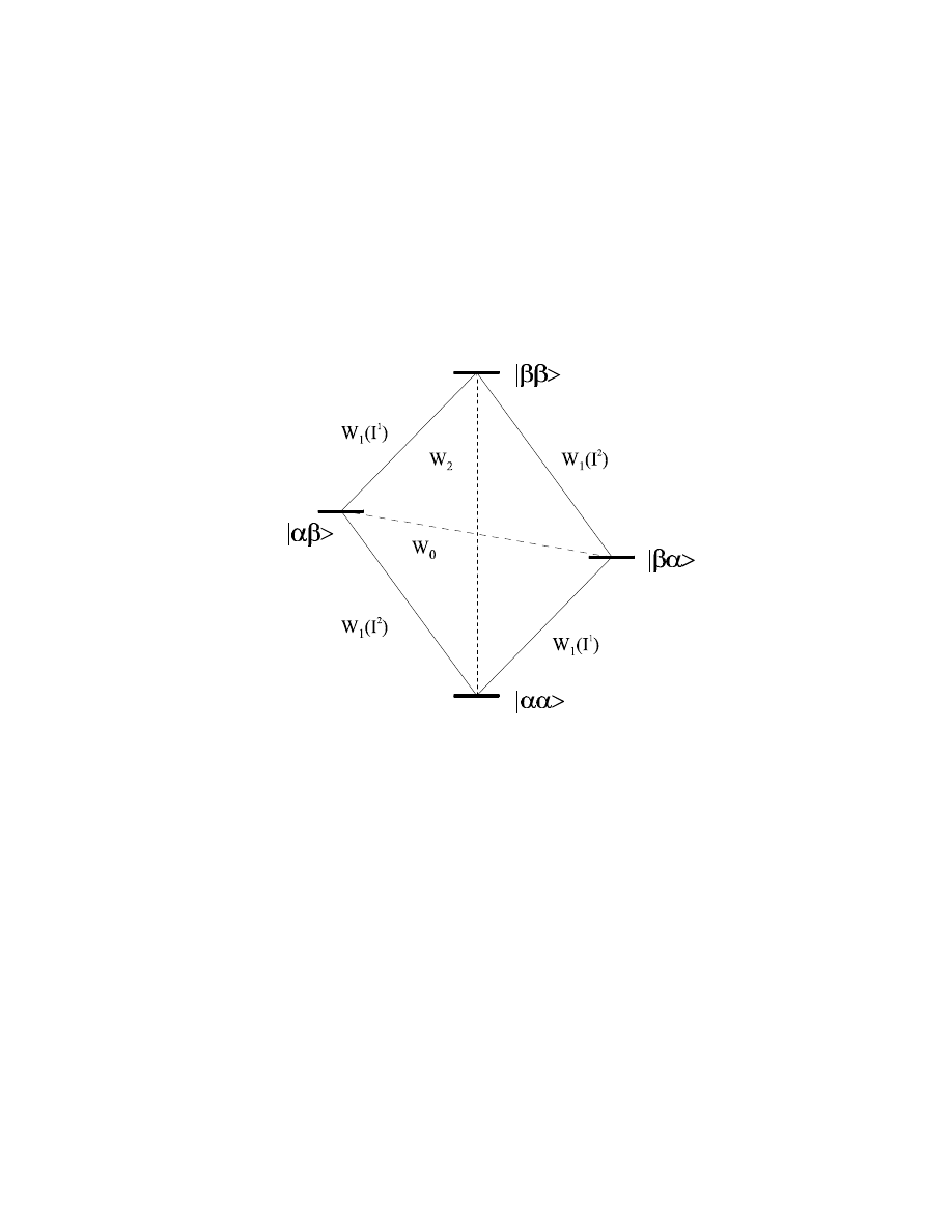
To understand the nature of the NOE, we have to look at a two-spin system I
1
and I
2
. Since NOE
does not involves coherences, but merely polarization, i.e. population differences between the
α
and
β
states, we can use the energy level diagram here:
The possible transitions for this two-spin system can be classified into three groups:
- W
1
transitions involving a spin flip of only one of the two spins (either I
1
or I
2
), corresponding
merely to T
1
relaxation of the spin.
- a W
0
transition involving a simultaneous spin flip
α→β
for one spin and
α→β
for the other one
(i.e., in summa a zero-quantum transition).
- a W
2
transition involving a simultaneous spin flip of both spins in the same direction,
corresponding to a net double-quantum transition.
We are just contemplating spin state transitions here caused by relaxation, which do not involve a
coherent process (like, e.g., I
x
/ I
y
coherences, which require a phase coherent transition between two
states that is generated by an r.f. pulse)!
93
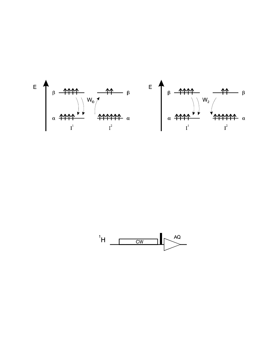
If we perturb one spin, e.g., I
1
, i.e., change its populations of the
α
and
β
state (e.g., by saturating the
resonance = creating equal population of both states), then relaxation will force I
1
back to the
equilibrium B
OLTZMANN
distribution. With the W
1
mechanism, spin I
1
will just relax without effecting
spin I
2
. However, the other two mechanism will effect I
2
:
With the I
1
polarization going back from saturation to the B
OLTZMANN
equilibrium, the W
0
mechanism will cause the neighbouring (so far unperturbed) spin to deviate from its B
OLTZMANN
equilibrium towards a decrease in
α,β
population difference. After a 90° pulse, this will result in a
decrease in signal intensity for I
2
— a "negative NOE effect".
On the other hand, the W
2
mechanism will cause the population difference of the undisturbed spin I
2
to increase, corresponding to an increase in signal intensity: a "positive NOE effect".
These effects can be directly observed in a very simple experiment, the 1D difference NOE sequence:
One spin is selectively saturated by a long, low-power CW (continuous wave) irradiation. As soon as
the spin deviates from its B
OLTZMANN
population distribution, it starts with T
1
relaxation. Via the W
0
or W
2
mechanisms it causes changes in the population distribution of neighbouring spins. After a 90°
pulse, these show up as an increase or decrease in signal intensity.

94
Usually, the experiment is repeated without saturation, giving the normal 1D spectrum. This is then
subtracted from the irradiated spectrum, so that the small intensity changes from the NOE effects can
be easier distinguished: spins with a positive NOE (i.e., higher intensity in the NOE spectrum than in
the reference 1D) show a small positive residual signal, spins with a negative NOE yield a negative
signal, spins without an NOE cancel completely.
What determines if we see a positive or a negative NOE? First of all, an NOE requires that there is a
significant interaction between the magnetic dipoles of the two spins. Dipolar interactions drop of
very fast with distance, so a
1
H,
1
H NOE can only occur with a distance of <5-6 Å (500-600 pm).
Due to the very small energy differences between NMR spin states, a spontaneous transition from a
higher to a lower energy state is very improbable (with average lifetimes of several years for the spin
states!). All transitions have to be induced by electromagnetic fields which are in resonance, i.e., have
the right frequency corresponding exactly to the energy difference of the two spin states involved in
the transition.
For the W
1
transitions, this frequency is identical with the Larmor frequency of the spin that is
undergoing the spin flip, i.e., the resonance frequencies
ω
(I
1
) and
ω
(I
2
) . For the W
0
transition, the
energy difference is identical to the difference
ω
(I
1
) –
ω
(I
2
) , and for W
2
it is the sum of the
resonance frequencies for the two spins,
ω
(I
1
) +
ω
(I
2
) .
If we consider, e.g.,
1
H in a 500 MHz spectrometer, then the W
1
mechanism would require
frequencies of 500 MHz to induce transitions, the W
2
mechanism (corresponding to a simulatneous
flip of two
1
H spins) requires fields of 1000 MHz, and the W
0
transitions frequencies equal to the
resonance frequency difference between the two protons, i.e., a few ppm (some 100 or 1000 Hz).
Where do we get these electromagnetic fields? If we imagine two small magnets (e.g., compass
needles) close together at a fixed distance (like two
1
H spins in a molecule) in an external magnetic
field (e.g., the Earth's magnetic field), then the interaction between the two depends on the orientation
of the "molecule" in the external field:
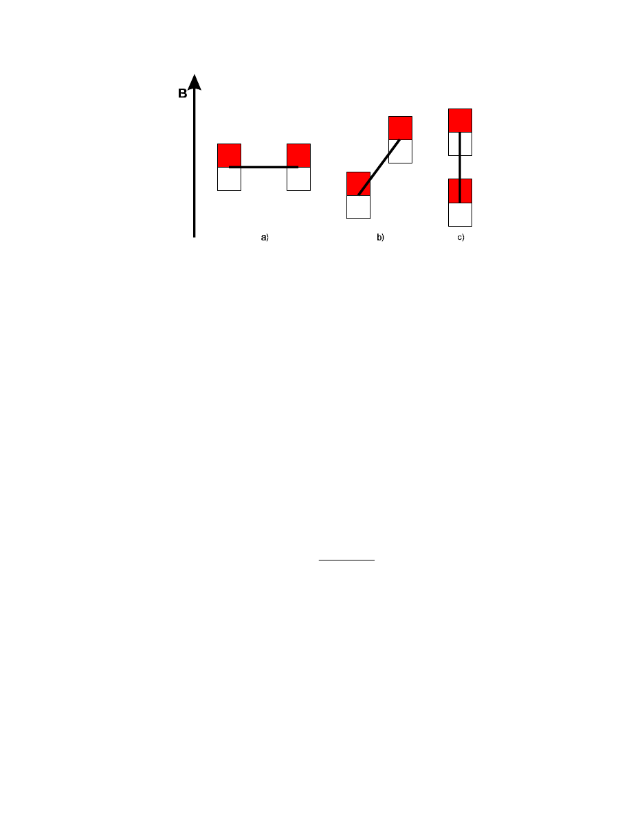
95
In position a), there will be a repulsive interaction between the two, in position c) it will be attractive,
and somewhere in between (position b)) the interaction will be zero. Now our molecule is not static,
but pushed around all the time in our sample solution. A rotation of the molecule will change its
orientation in the static magnetic field and cause a modulation of the field strenght a spin actually
"experiences" – through the effects of the neighbouring spins. Thus, the rotation of the other spins
generates an electromagnetic field – just like in an electric generator, but not with a well-defined
frequency, but with a wide range of frequency components, due to the random nature of the
molecular rotation.
The easiest approximation to describe the rotation of a molecule in solution is the assumption of the
molecule as a rigid sphere. If we calculate how "much" of a certain frequency is generated in the
random rotation, we find the following expression for the "spectral density" at a frequency
ω
:
J
c
c
( )
ω
τ
ω τ
=
+
2
1
2
2
It means that we have a maximum at
ω
=0 and the spectral density then drops off for higher
frequencies. How fast is controlled by the parameter
τ
c
, the molecular rotaional correlation time (or
just "correlation time"). A long correlation time means a rather sluggish rotation, and a fast drop off
of J (=very small high-frequency contributions). A short
τ
c
corresponds to a fast random rotation,
causing a much wider frequency distribution / more high-frequency contributions.
96
The correlation time is determined by different factors: mainly, the molecular weight. The larger a
molecule, the slower its re-orientation, i.e., the longer its
τ
c
. As a rule-of-thumb, the correlation time
of a molecul can be estimated from the molecular weight MW:
τ
c
[ps]
≈
0.5 MW [Da] (e.g., a MW
of 1000 Da corresponds to ca. 0.5 ns). But
τ
c
is also influenced by other parameters: temperature (the
higher the temperature, the shorter
τ
c
), solvent viscosity (the more viscous, the longer
τ
c
),
aggregation in solution etc..
Back to the NOE: the observable NOE is determined by the cross-relaxation rate
σ
= (W
2
- W
0
)
and with the dependence on the spectral densities at the "resonance frequencies" for W
0
(
ω
≈
0) and
W
2
(
ω
= 2
ω
0
) we get:
σ
ω
ij
ij
r
J
J
∝
−
1
6
2
0
6
0
{
(
)
( )}
For 6J(2
ω
0
) > J(0)
, we get positive NOEs. This requires a relatively high spectral density at
ω
= 2
ω
0
, i.e., a short
τ
c
. In the opposite case (long
τ
c
), W
0
will dominate: negative NOEs. The crossing
point is at
ω
0
τ
c
=
5
2
≈
1 , where the effects from W
0
and W
2
cancel each other and there is no
NOE to be observed.
In these equations we are looking at
σ
ij
, the cross-relaxation rate between two spins i and j .
However, in the 1D difference NOE experiment described above, we cannot really measure the rate
of NOE build-up, since we need a relatively long (in the order of seconds), low-power selective
irradiation to saturate one spin. During this time, the NOE will gradually build-up, as we start
saturating I
1
more and more, with no defined starting point. What we get after sufficiently long
irradiation is the so-called "steady state NOE", i.e. the steady state population distribution of the
neighbouring spins that derives from two counter-acting effects: 1. the NOE build-up from cross-
relaxation with the irradiated spin I
1
, and 2. the T
1
relaxation of the spins that have deviated from
their B
OLTZMANN
equilibrium due to the NOE, trying to bring them back to the equilibrium state.

97
The steady state NOE resulting from this balance now does not relly depend on the distance between
the two spins, only so far that the observation of any effect proves the distance to be shorter than ca.
5-6 Å. The intensity of the observed NOE can vary widely, depending on the neighbourhood of other
protons which act as a relaxation source. A few examples will show this (from: Sanders / Hunter,
Modern NMR Spectroscopy, Oxford University press, Oxford 1987):
two-spin system I
1
– I
2
I
1
I
2
saturated
50 %
for small molecules (W
2
dominating)
50 %
saturated
saturated
-100 %
for large molecules (W
0
dominating)
-100 %
saturated
There is no distance dependence for these steady-state NOEs!
linear three-spin system I
1
– I
2
– I
3
(r
23
= r
12
) *
I
1
I
2
I
3
saturated
25 %
-11.5 %
49.2 %
saturated
49.2 %
-11.5 %
25 %
saturated
*only shown for positive NOEs, with W
2
>> W
0
!
Generally, the NOEs are weaker, because they now have to compete with relaxation from two
neighbouring protons. This can be seen esp. for the first case, where I
2
gets an NOE contribution
from the saturated spin I
1
, but now has two equally close neighbours causing T
1
relaxation (I
1
and I
3
).
Since the NOE on I
2
leads to an increased population difference for this spin, it causes itself (being
98
not in the B
OLTZMANN
equilibrium anymore) an NOE at spin I
3
, of opposite sign than the direct
NOE caused by the decreased population difference of I
1
.
linear three-spin system I
1
– I
2
–––– I
3
(r
23
= 2 r
12
) *
I
1
I
2
I
3
saturated
49.2 %
-18.6 %
50 %
saturated
50 %
-0.4 %
0.8 %
saturated
*for W
2
>> W
0
!
In the last case, I
1
and I
2
are close together and relax each other very efficiently, while the NOE
build-up from the more distant I
3
is too slow to lead to a significant staedy state NOE. This is often
true,e.g., for CH
2
groups, where the distance between the two methylene protons (ca. 1.78 Å) is
much shorter than to any other proton.
2D NOESY
Any quantitative interpretation of steady state NOEs requires knowledge of the arrangement of all
protons relative to each other! Otherwise, instead of staedy state NOEs, the NOE build-up rate has to
be determined, which depends on the interproton distance with r
–6
. It is also called the transient
NOE or kinetic NOE.
While some variations of the 1D difference NOE experiment have been used to measure build-ip
rates, the easiest way to do this is the 2D NOESY experiment:
Like, e.g., the 2D COSY or TOCSY experiments, it starts with a
1
H 90° pulse followed by a
1
H
indirect evolution time, at the end of which the following terms exist:

99
I
1x
cos
Ω
1
t
1
cos
π
Jt
1
+ I
1y
sin
Ω
1
t
1
cos
π
Jt
1
+ 2I
1y
I
2z
cos
Ω
1
t
1
sin
π
Jt
1
– 2I
1x
I
2z
sin
Ω
1
t
1
sin
π
Jt
1
100
After the 90°
y
1
H pulse at the end of t
1
we get
–I
1z
cos
Ω
1
t
1
cos
π
Jt
1
+ I
1y
sin
Ω
1
t
1
cos
π
Jt
1
+ 2I
1y
I
2x
cos
Ω
1
t
1
sin
π
Jt
1
+ 2I
1z
I
2x
sin
Ω
1
t
1
sin
π
Jt
1
polarization
SQC
DQC+ZQC
SQC
The phase cycle is set up so that only coherences with coherence order zero during
τ
m
are selected,
i.e., the first term (polarization) and the ZQC part of the third term (= I
1y
I
2x
– 2I
1x
I
2y
).
The first term is a z magnetization which is modulated with the cosine of the chemical shift (and
coupling), i.e., it oscillates between +I
1z
and –I
1z
. This non-equilibrium polarization will cause an
NOE on neighbouring protons:
–I
1z
cos
Ω
1
t
1
cos
π
Jt
1
→
– (1-k
12
) I
1z
cos
Ω
1
t
1
cos
π
Jt
1
– k
12
I
2z
cos
Ω
1
t
1
cos
π
Jt
1
The amount of NOE transfer is, of course, determined by the cross-relaxation rate
σ
12
and the
duration of
τ
m
. After the final
1
H 90° pulsethese z components are converted into detectable signals:
→
– (1-k
12
) I
1x
cos
Ω
1
t
1
cos
π
Jt
1
– k
12
I
2x
cos
Ω
1
t
1
cos
π
Jt
1
The first term results in a diagonal peak after 2D FT (at
Ω
1
) , the second one in a cross-peak at
Ω
1
in
F1 (from the t
1
modulation) and at
Ω
2
in F2 (since it is an I
2
coherence now). The sign of the cross-
peak depends on the sign of the cross-relaxation rate, i.e., the dominance of either W
0
or W
2
(the
diagram shows the maximum NOE cross-peak
intensity relative to the diagonal system):
- with a negative NOE effect, the cross-peaks will
be negative with a negative diagonal signal (like
in the 1D difference NOE experiment!)
- for a positive NOE effect, one gets positive
cross-peaks (with a negative diagonal).
- for
ω
0
τ
c
≈
1, the NOE effect will disappear, and
no NOESY cross-peaks will be visible
101
Unfortunately, the ZQC term will also survive the phase cycling, and lead to dispersive antiphase
signals at the diagonal and at the cross-peak position between two protons with a scalar coupling.
These signals can feign a NOESY cross-peak even in the absence of an NOE!
However, unlike the in-phase NOE cross-peaks, they do not have a net integral (antiphase!), so that
they can be distinguished from real NOESY cross-peaks (but only if really the whole peak area is
integrated, including the wide dispersive tails of the ZQC poeaks!). Of course, ZQC peaks do not
interfere with an NOE between two protons that do not show a mutual scalar coupling!
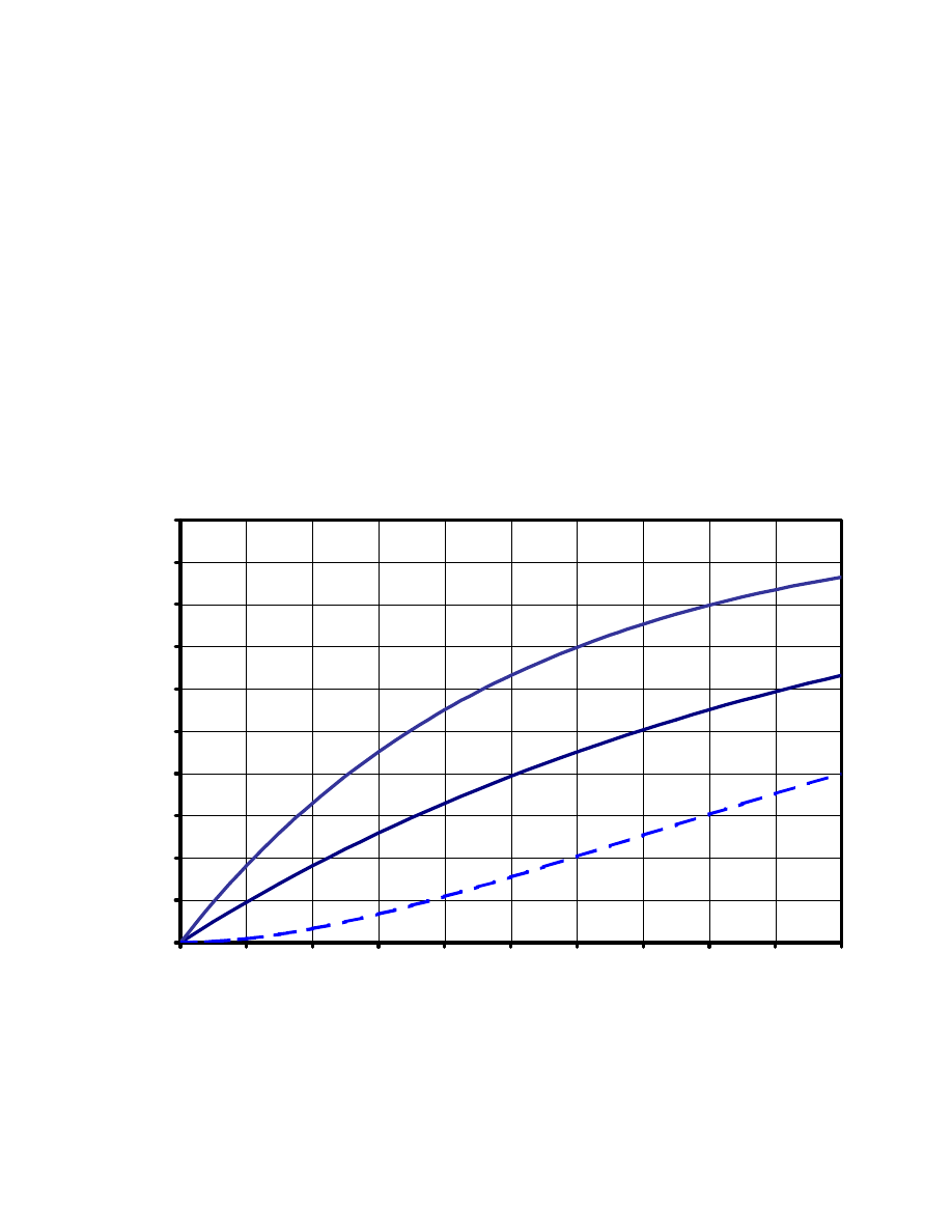
How does one now measure
σ
ij
, i.e., the NOE build-up rate? Let's consider the behaviour of the
NOE (i.e., the integral of the NOESY cross-peak) as a function of
τ
m
:
0.0
0.1
0.2
0.3
0.4
0.5
0.6
0.7
0.8
0.9
1.0
0.0
0.1
0.2
0.3
0.4
0.5
0.6
0.7
0.8
0.9
1.0
τ
m
[s]
NOE (arbitrary units)
Here, the build-up of two NOEs is shown (solid lines), with the
σ
of the first one twice as large as the
second one. In addition, an indirect NOE (i.e., an NOE caused by the perturbation from a direct
NOE) is depicted with a broken line.

102
Obviously, the build-up of the two direct NOEs is only proportional to their
σ
values for
τ
m
=0 , at the
very beginning of the curves, which then deviate more and more from a straight line to reach some
sort of plateau for very long
τ
m
values. This initial slope of the NOE build-up curve corrsponds to the
cross-relaxation rate
σ
, which depends on the interproton distance!
It can be measured in two ways:
- by measuring 2D NOESYs with a series of increasing
τ
m
delays (e.g., at 50, 100, 200, 300 ms),
and then fitting an exponential function to the data points extrapolating down to
τ
m
=0. This will
give very reliable results, but require a lot of spectrometer (and processing and evaluation time).
- or by measuring just a single 2D NOESY experiment with a sufficiently short
τ
m
, so that the
build-up curves can still be considered linear in good approximation (in our example, with
τ
m
≤
100 ms). This will be much easier than actually tracking the whole build-up curve. The
problem, however, lies in the term "sufficiently short". If one chooses
τ
m
too short, then the
NOE cross-peak intensities will be just too low to measure; if
τ
m
is not short enough, then the
measured intensities will show considerable deviations from the
σ
ratios! Solution: either
measure the whole build-up curve once and assume that it will be similar for all molecules with
similar
τ
c
(i.e., similar molecular weight at similar temperature and solvent). Or: take an
educated guess (e.g., from
τ
m
values given in the literature)…
Indirect NOEs can be recognized by their initial slope, which is zero! This means that they only show
up at longer mixing times. However, when a "sufficiently short" mixing time is chosen still too long,
they can be mistaken for "real" direct NOEs.
If all these precautions are kept in mind, NOEs (=cross-peak integrals) can be converted into
interproton distances. This is usually be done with the help of a reference NOE corresponding to a
known distance (e.g., CH
2
groups, H-C-C-H fragments in aromatic rings etc.):
r
r
I
I
ij
ref
ref
ij
=
6
103
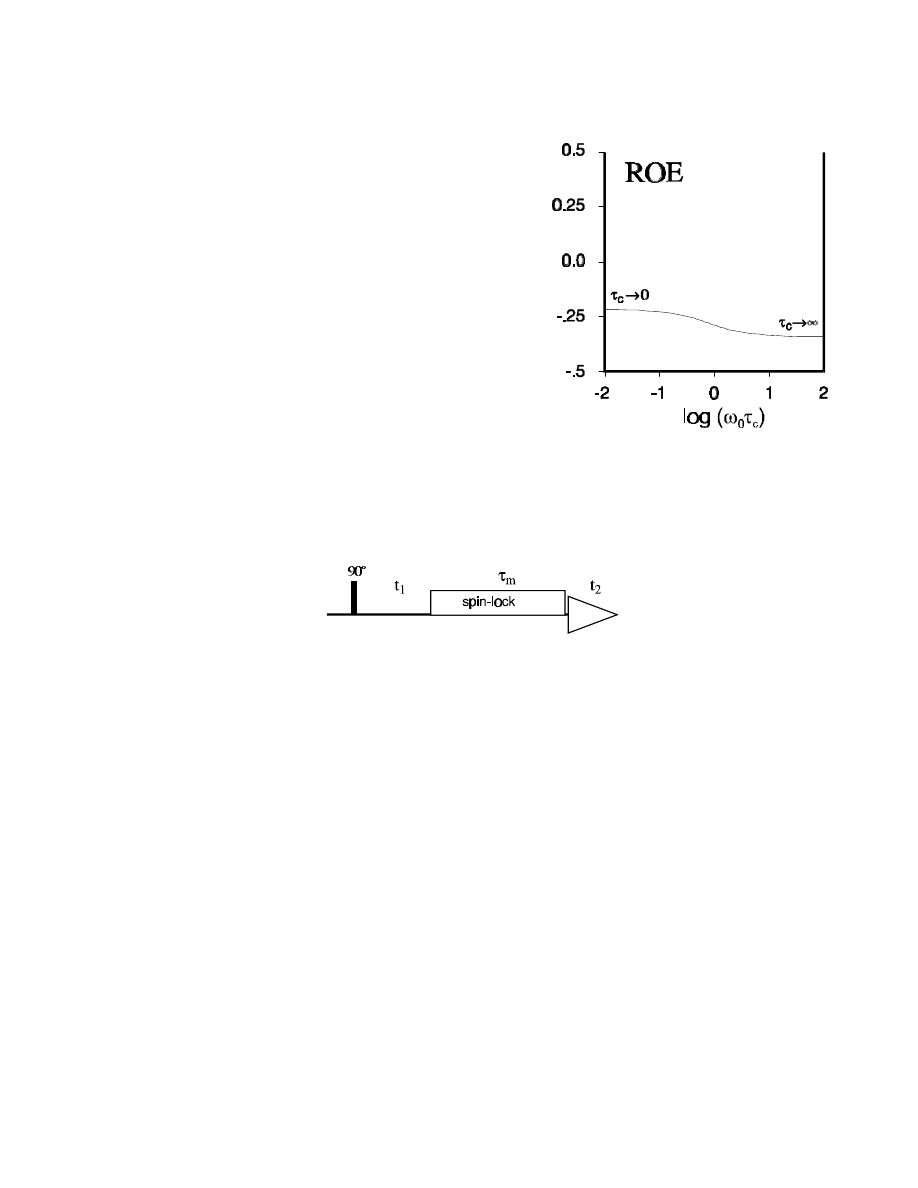
2D ROESY
When the correlation time is close to
τ
c
=
1
/
ω
0
, then no
NOE effects will be observable. However, there is a
modification of the NOESY experiment with a different
dependence of the NOE on
ω
0
τ
c
:
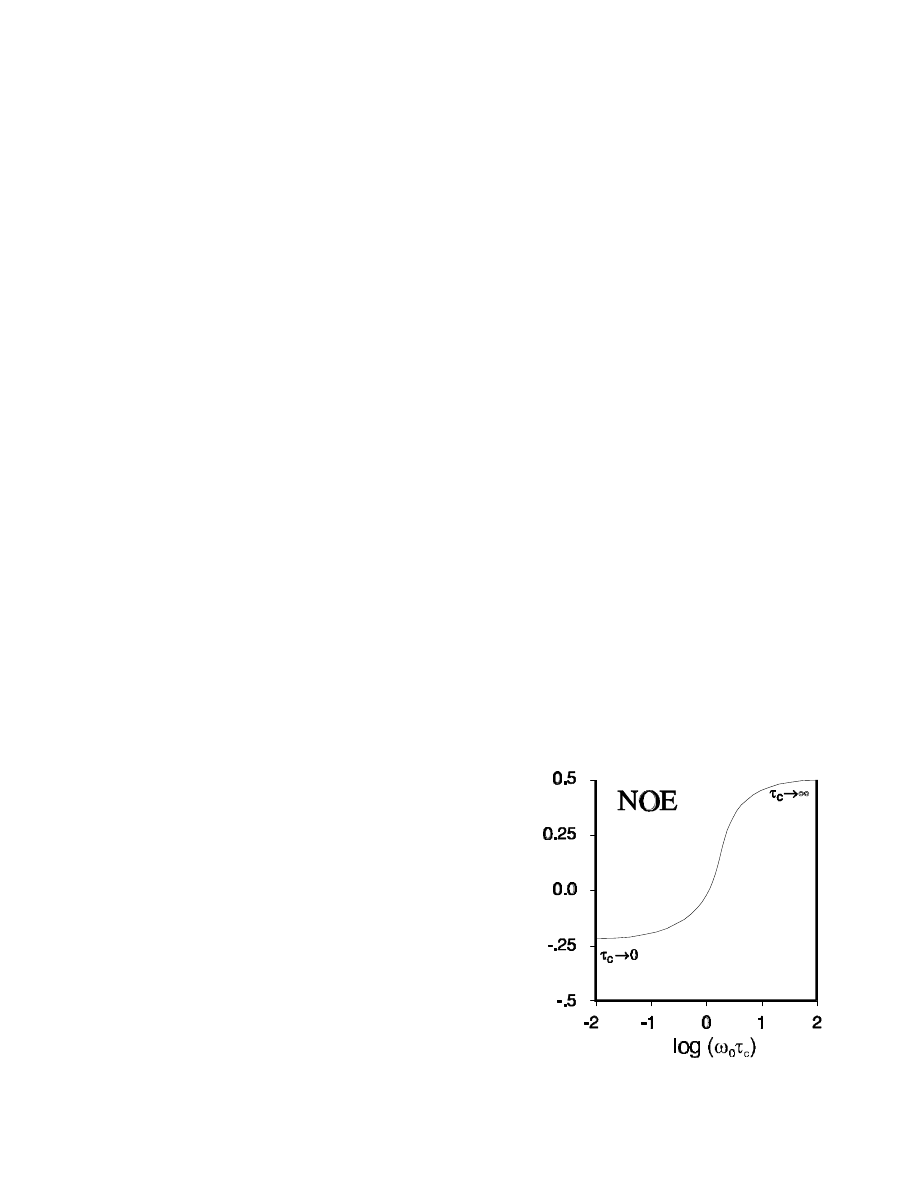
In the ROESY (=Rotating frame NOESY) experiment,
the NOE (or better, the ROE) is always positiv, i.e., the
ROE cross-peaks have the opposite sign as the diagonal
peaks. And it never becomes zero!
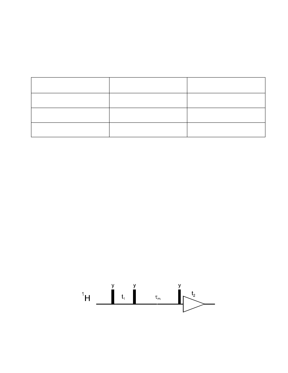
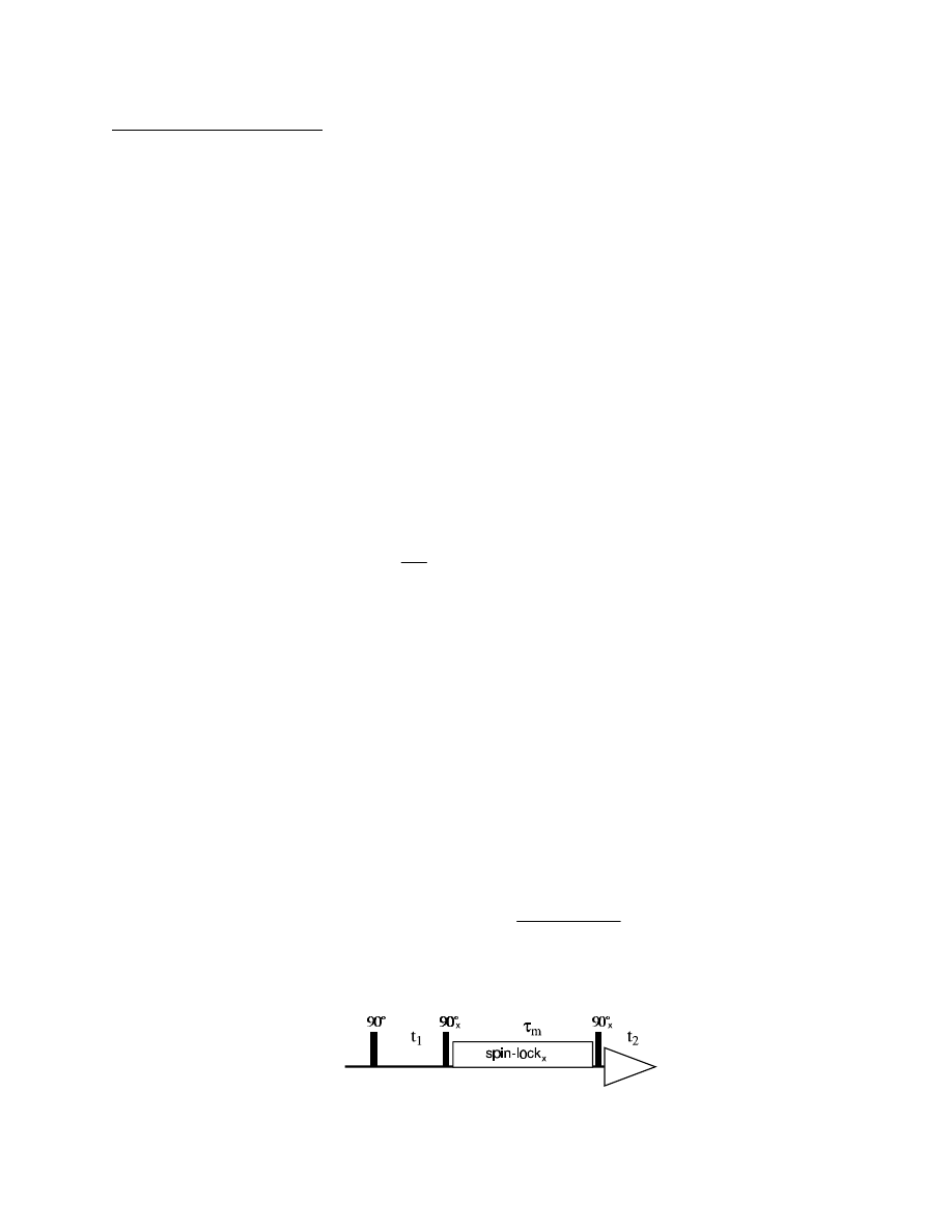
The pulse sequence for the ROESY experiment is relatively simple: it is identical to the TOCSY
sequence! After the first 90° pulse and the t
1
time, a spin-lock sequence follows during which the
ROE builds up, exactly as the NOE during the mixing time
τ
m
of the NOESY.
In the ROESY experiment, relaxation does not occur in the static B
0
field along the z axis, but in the
transverse field generated by the r.f. irradiation: the non-equilibrium transverse component (e.g., I
1x
)
relaxes with T
1
ρ
while "frozen" in the spin-lock field, thereby generating a transverse component I
2x
in
neighbouring spins by cross-relaxation.
With the exception of the different dependence on correlation time, everything else works like for the
NOE: again, the initial ROE build-up rate shows a r
-6
dependence, but with longer mixing (=spin-
lock) times, the build-up becomes non-linear, and indirect ROEs start to occur. And, like in the
NOESY, dispersive antiphase peaks can occur that are not caused by ROE, but by scalar coupling.
However, while the NOESY experiment is rather straightforward to evaluate, there are several
additional problems to be considered with the ROESY:
−
offset dependence of the ROE and interference between NOE and ROE,
−
TOCSY contributions in the ROESY spectrum.
104
Offset effects in the ROESY
Due to the very limited power of the r.f. spin-lock fields (a few kHz, compared to several hundred
MHz for the static field), an efficient spin-lock in the transverse x,y plane occurs only close to the
resonance frequency of the irradiated field (usually in the center of the spectral window). Towards the
edges of the spectrum, the spin-lock field becomes to weak to force the spins into a precession about
its transverse axis. As a result, the spins precess about an effective axis that gradually tilts from the x,y
plane (on resonance) back to the z axis of the static field (far off-resonance).
This has several consequences:
−
off resonance, the efficieny of the ROE drops off with sin
θ
i
sin
θ
j
for the ROE from proton i to
proton j, where
θ
is the angle between the spins' precession axis and the x,y plane. This angle can
be calculated for each spin from the ratio between the frequency offset (causing a precessing about
the z axis) and the spin-lock field (causing the x,y precession component):
θ
γ
i
i
B
∝
arctan
Ω
1
where
Ω
i
is the offset of the spin from on-resonance and
γ
B
1
the field strength of the spin-lock field
(both in Hz).
−
since we go into the spin-lock field with pure transverse magnetization of spin i (from the initial
90° pulse), we add another factor sin
θ
i
, since we can only lock the magnetization parallel to the
spin-lock axis. Similarly, we have to add another sin
θ
j
when we detect the resulting spin j
magnetization during t
2
, since we can only see the x,y component of the spinlocked magnetization.
All this means that our measured ROE
exp.
has to be corrected to get the true ROE correlated with
the interproton distance:
ROE
ROE
true
ij
ij
i
j
=
exp.
sin
sin
1
2
2
θ
θ
A "compensated ROESY" version has also been introduced, with a weaker offset dependence:
Here the required correction for the cross-peak integrals is
105
ROE
ROE
true
ij
ij
i
j
=
exp.
sin
sin
1
θ
θ
For all these offset corrections one needs to know just the spin-lock field strength used in the
ROESY experiment, then the correction can be calculated automatically for each cross-peak
individually!
Interference of NOE and ROE
For
ω
0
τ
c
≈
1, where there is no significant NOE, this is all the correction that we need. However, if
that is not true, then we will simultaneously get NOE contributions from the z components of the
spinlocked magnetization (off-resonance, where the spin-lock axis tilts away from the transverse
plane). So, the result of cross-relaxation during the spin-lock mixing time will be a combination of
ROE and NOE:
σ
ij
= ROE
ij
sin
θ
i
sin
θ
j
+ NOE cos
θ
i
cos
θ
j
(in addition, all this is also multiplied with another sin
θ
i
sin
θ
j
for the projection onto the spin-lock
axis and back).
This is a severe complication because it depends not only on the easily calculated individual offsets
in F1 and F2 (via the
θ
values), but also on the ratio between NOE and ROE, which depends on
the exact correlation time
τ
c
of the molecule.
Only for the extreme cases this correction is still relatively easy:
ω
0
τ
c
>> 1 :
NOE : ROE = 1
ω
0
τ
c
<< 1 :
NOE : ROE = -2
For the sake of simplicity, ROESY spectra should only be quantitatively evaluated when there is no
significant NOE observed under the same conditions!
TOCSY contributions
... yet another complication in ROESY spectra! The pulse sequences for ROESY and TOCSY are
virtually identical, therefore it is obvious that TOCSY transfer will also be observed in a ROESY
experiment. This will, of course, only affect protons which have a mutual sclar coupling!

106
Since TOCSY cross-peaks are also in-phase, but of the opposite sign as ROESY cross-peaks
(TOCSY: same sign as diagonal peaks; ROESY: opposite sign as diagonal), they will partially cancel
the ROESY cross-peak intensities, leading to distances that are too long. However, when the cross-
peak used for distance reference contains a large TOCSY contribution (as do all CH
2
peaks!), then
the other cross-peaks appear too intense, resulting in distances that are too short.
Luckily, TOCSY contributions can be minimized by choosing an appropriate spin-lock sequence. The
TOCSY transfer relies on perfect synchronization of the two spins involved, while the non-coherent
ROESY cross-relaxation is much more robust with respect to imperfect alignment of the two spins
during
τ
m
. This leads to the following possibilities for suppression of TOCSY contributions:
choose a weak spin-lock field, typically 2-4 kHz (depending on spectral width in Hz to be covered,
i.e., spectrometer frequency)! For the ROESY transfer, this will only cause a faster decrease of cross-
peak intensities from the center of the spectrum towards its edges (cf. equation for
θ
). For the
TOCSY transfer, the performance drops dramatically (usually spin-lock fields of 8-10 kHz are used).
choose a "bad" spin-lock sequence instead of the optimized sequences used for a TOCSY (MLEV,
WALTZ, DIPSI). Good results can be achieved, e.g., with just continuous (CW) irradiation, or
thousands of evenly spaced short pulses (<< 90°, equivalent to a CW spin-lock). A spin-lock
consisting of just a train of 180° pulses with inverted phase ( - 180°
x
- 180°
-x
- ) also works well.
Even with these "poor" spin-lock sequences, there are still certain regions in the spectrum where
cross-peaks might contain significant TOCSY contributions:
close to the diagonal (again affecting especially CH
2
groups) with all spin-lock sequences, and
also close to the counter-diagonal crossing the diagonal in the center under a 90° angle.
(The spin-lock sequence of alternating 180° pulses does not produce TOCSY peaks along the
counter-diagonal, but pretty severe ones along the diagonal).
If an important cross-peak (involving two protons with a scalar coupling!) would fall onto the
counter-diagonal, the spectral window can be slightly shifted, so that the transmitter frequency is
moved away from the center between the two protons, and the potential ROESY cross-peak does not
fall onto the counter-diagonal anymore.
For two peaks with very close resonance frequencies (cross-peak close to the diagonal), TOCSY
contributions cannot be avoided!

107
Table comparing important features of NOESY and ROESY spectra
NOESY
ROESY
NOEs depend strongly on correlation time,
vanish for
ω
0
τ
c
≈
1
only weak dependence on correlation time,
ROE always present
NOE cross-peaks same sign as diagonal (for
negative NOEs) or opposite sign (for positive
NOEs)
ROEs always positive, i.e., opposite sign
compared to diagonal
peaks from chemical exchange show same
sign as diagonal: easily distinguishable from
positive NOEs, but can be confused with
negative NOEs
peaks from chemical exchange show same
sign as diagonal: easily distinguishable from
always positive ROEs
no offset effects, integrals can be directly
used
offset effects have to be corrected
no ROESY contributions
interference with NOESY contributions
except for
ω
0
τ
c
≈
1 (vanishing NOE)
antiphase ZQC cross-peaks from scalar
coupling confusing, but don't interfere with
NOESY cross-peak integrals
TOCSY contributions from scalar coupling
can change ROESY peak integrals, resulting
in distance errors
Wyszukiwarka
Podobne podstrony:
Herbert, Frank The GM Effect
Brunner, John The Pronounced Effect
Al Mann The Trionym Effect
Wigner The Unreasonable Effectiveness of Mathematics in the Natural Sciences
Frank Herbert Destination Void 03 The Lazarus Effect
The Most Effective Way to Utilize Fibonacci Ratios
62 The Domino Effect
Intoxication Anosognosia The Spellbinding Effect of Psychiatric Drugs Peter R Breggin, MD
The Hipster Effect When anticonformists all look the same
Comparative assessment of the energy effects of biomass combustion
Brunner, John The Pronounced Effect
The SLI Effect Street Lamp Interference A Provisional Assessment comp by Hilary Evans & ASSAP (200
The Two Effects of the Gospel
73 The butterfly effect
Frank Herbert Destination Void 3 The Lazarus Effect
Frank Herbert The GM Effect
Herbert, Frank DV 3 The Lazarus Effect
Heider, The Rashomon Effect
The Daleth Effect Harry Harrison
więcej podobnych podstron