Getting Started With ANSYS:
TIPS
www.ansys.belcan.com
by Paul Dufour
Introduction:
ANSYS is a sophisticated and comprehensive finite
element program that has capabilities in many different
physics fields such as static structural, nonlinear, thermal,
implicit and explicit dynamics, fluid flow,
electromagnetics, and electric field analysis. It can also
perform coupled field analysis combining one or more of
these different physics. Obviously because ANSYS is s
a huge program with so many capabilities (even within
one of these physics fields) it is impossible to cover
everything in this short guide. This document will give an introduction as to how the ANSYS progra
works and how these basic skills will be applicable to any type of analysis within ANSYS. The most
important concepts in using ANSYS will be addressed here in a compressed format. The key to
becoming productive in any computer aided engineering program is to start to think like the program
thinks, to get the big picture of how it works in general. That is the primary goal of this guideline.
uch
just
m
A Couple of Preliminaries:
ANSYS is an integrated program with all operations performed under one GUI. Creating the model,
running it, and postprocessing the results are all done without leaving the ANSYS environment.
There are several different ways of working within ANSYS. This stems from the fact that like every
program, ANSYS is driven by commands. The difference between ANSYS and say, Microsoft Word,
is that when you click on an icon in Word, you have no idea what command was executed behind the
scenes to make the program do what you asked. ANSYS gives you easy access to these commands if
you want to use them. These commands are simple to use; just a keyword followed by several
arguments. By stacking these commands together in a text file the power to automate and script
ANSYS is one key reason why I think it is superior to other FEA codes on the market. More on this
powerful scripting capability in a later section.
New ANSYS users generally don’t care much about scripting to start with and just want to figure out
how to do what they want within the GUI environment, and that’s where we will start as well. Each
key concept will be explained as succinctly as possible, then at the end we will do a simple problem
using several different approaches to put it all together.
Starting ANSYS:
When you start ANSYS from the Windows Start Menu you
get three basic choices.
ANSYS Workbench: This is a brand new GUI with an emphasis on CAD connectivity, ease of use, and
easy management of assembly contact. This GUI is covered in a separate guideline.
Copyright 2003 Belcan Engineering Group, Inc.
1
ANSYS: This starts ANSYS in the traditional GUI. The program starts immediately using the settings
last changed under the next item, “Configure ANSYS Products”. This guideline will cover this GUI.
Configure ANSYS Products: This sounds like something you might use only the first time you fire up
ANSYS, but surprise! Typically this is where you will start the program from every time. This choice
brings up what has been always called the ANSYS Launcher.
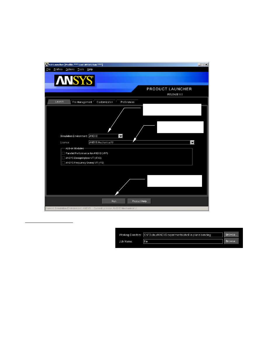
Pick your environment: ANSYS
or Workbench, or batch mode.
Any license you have
paid for shows up here.
Start your ANSYS session
with the specified parameters.
File Management Tab:
All files created in this session will be
called
jobname.something
, and be
created in the working directory
specified here. The default jobname is
“file”. I like to organize my work by different directories and always use the jobname “file”, but this is
a personal preference.
Key ANSYS files you need to know about:
jobname.db
– This is your database, where your model is stored.
jobname.dbb
– When you save, your existing database file is copied to this before actually saving as a
backup.
jobname.log
– Everything you do in a session is written to this file in the form of commands.
jobname.rxx
– Results file.
xx = st
for structural,
xx = th
for thermal, etc.
Copyright 2003 Belcan Engineering Group, Inc.
2
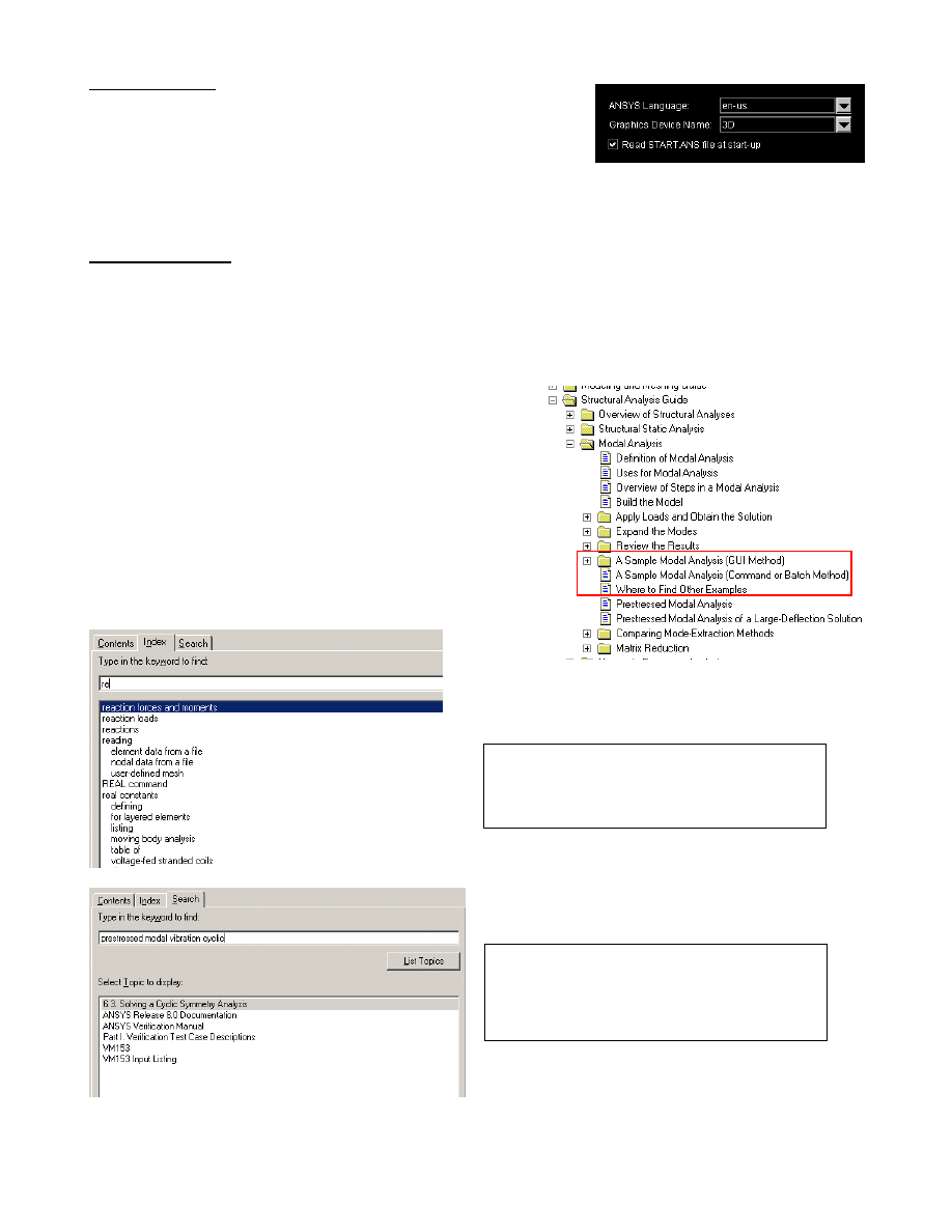
Preferences Tab:
The 3D graphics driver allows you to rotate a shaded view of
your model. Most newer graphics cards can handle this fine.
Under the “Profiles” pull down menu you can save settings and easily recall them to quickly start
ANSYS with specific settings that you have defined previously.
The Help System:
ANSYS has excellent documentation available under the help menu in the main GUI window. The
amount and comprehensiveness of information available under the help menu is both a blessing and a
curse. What you want to know is there, but at times it’s hard to dig out due to the sheer amount of
information. A couple of hints:
Use the tutorials found under “Help
→ ANSYS
Tutorials”. There are nine different tutorials here that
are step by step, mouse click by mouse click instructions
for various types of analysis.
Under the Analysis Guide for each discipline, there are
also step by step instructions with explanations on how
to do each type of simulation. These are well
done…take advantage of them!
Under the Index tab start typing and it will
jump to that section of the list of topics as
shown at left.
When searching, use more than one word
to narrow down the search. To search on
a specific phrase put the words in double
quotes.
Copyright 2003 Belcan Engineering Group, Inc.
3
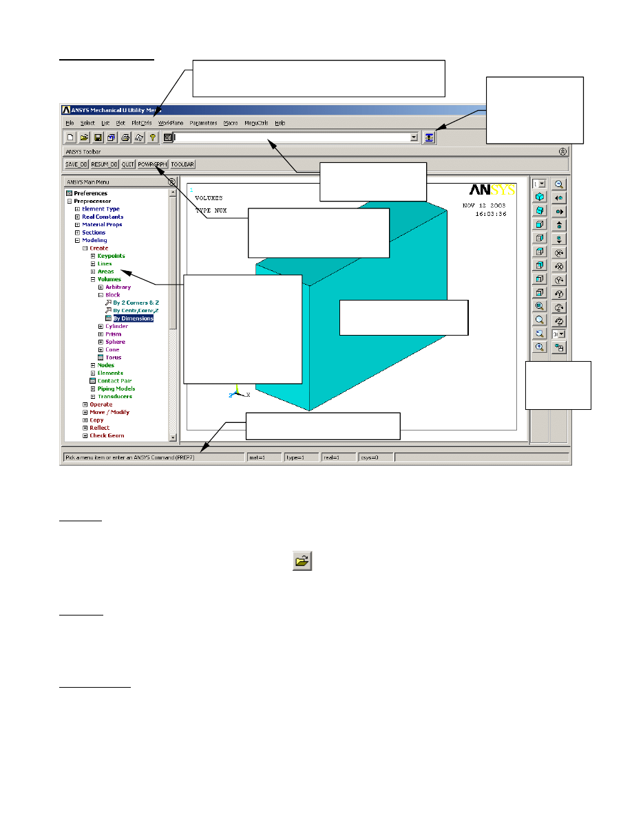
The ANSYS GUI:
Graphics window. This is
where you “plot” things to the
screen.
Manipulate
your model
view with
these buttons.
The Main Menu. Nodes of
the tree expand and
contract. If you collapse a
full branch, it remembers
where you were upon
reopening, so you don’t
have to re-drill down to get
to that item.
Can type in ANSYS
commands here if you
know them.
Customize this toolbar with
frequently used commands or
create push button automation
with macros assigned to a button.
Utility menu. These are ancillary functions that are not
directly related to creating, solving and selecting results to
look at for your finite element model.
Raise hidden. If a
dialog disappears
behind the main
window, bring it back
with this.
Look at this! ANSYS will prompt
you for what to do next.
This GUI is fairly easy to use, however there is some “ANSYS-speak” related to basic operation:
Resume: This is opening a previously saved database. It is important to know that if you simply
resume a database, it doesn’t change the jobname. For example: You start ANSYS with a jobname of
“file”. Then you resume
mymodel.db
, do some work, then save. That save is done to
file.db
!
Avoid this issue by always resuming using the
icon on the toolbar. If you open
mymodel.db
using
this method, it resumes the model and automatically changes the jobname to
mymodel
.
Plotting: Contrary to the name, this has nothing to do with sending an image to a plotter or printer.
Plotting in ANSYS refers to drawing something in the graphics window. Generally you plot one type
of entity (lines, elements, etc.) to the screen at a time. If you want to plot more than one kind of entity
use, “Plot
→ Multiplot”, which by default will plot everything in your model at once.
Plot Controls: This refers to how you want your “plot” to look on the screen (shaded, wireframe,
entity numbers on or off, etc). Other plot control functions include sending an image to a graphics file
or printer.
Copyright 2003 Belcan Engineering Group, Inc.
4
Mouse Functionality:
Pressing the scroll wheel button is the same as a middle mouse button.
Picking Entities:
Left Button: Picks an entity. Picking is cumulative, so you don’t need to press control or shift to
pick more than one entity. Click and hold the button, then move the cursor around until the entity
you want is highlighted. When you release the button the highlighted entity is selected.
Middle Button: Completes a selection. This is like clicking “Apply” in the picking dialog (also
called “the picker”).
Right Button: Toggle back and forth between “pick” and “unpick” mode. Cursor changes so
you know what mode you in.
Manipulating the Model View: (you can change these defaults to different buttons if desired)
CTRL + Left Button: Pan the model side to side and up and down.
CTRL + Middle Button: Move the mouse left and right to rotate about screen Z. Up and down
zooms in and out.
CTRL + Right Button: Rotate the model.
Right Button: Click and drag the right button to zoom in using a window.
Rolling the scroll wheel also zooms in and out.
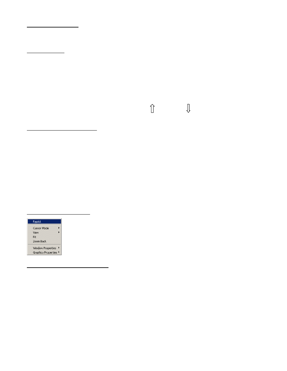
Right Button Pop-up Menu:
When you click the right button in the graphics area you get this pop-up with some
very common graphics functions.
• ANSYS does not always refresh the graphics screen so “Replot” is very handy.
• “Fit” makes your whole model visible.
• “Zoom Back” will go back to the view the way it was just before you zoomed in.
Importing or Creating Geometry:
Import CAD geometry using “File
→ Import”. ANSYS comes with IGES support by default but there
are Geometry Interfaces available for Pro/E, CATIA, UG, Solidworks, Parasolid, etc. IGES is the
oldest of these formats and does not work very well for solids, but is OK for wireframe geometry. All
of these geometry interfaces on the ANSYS “Traditional” side perform a translation of the geometry
into an ANSYS Neutral File (.anf) format, which it then reads in. In Workbench there is no
translation, it works with the native CAD format geometry.
Copyright 2003 Belcan Engineering Group, Inc.
5
Geometry in ANSYS is created from “Main Menu
→ Preprocessor → Modeling → Create” and has
the following terminology,
KEYPOINTS: These are points, locations in 3D space.
LINES: This includes straight lines, curves, circles, spline curves, etc. Lines are typically defined
using existing keypoints.
AREAS: This is a surface. When you create an area, it’s associated lines and keypoints are
automatically created to border it.
VOLUMES: This is a solid. When you create a volume, it’s associated areas, lines and keypoints are
automatically created.
SOLID MODEL: In most packages this would refer to the volumes only, but in ANSYS this refers to
your geometry. Any geometry. A line is considered a “solid model”.
You can’t delete a child entity without deleting its parent, in other words you can’t delete a line if it’s
part of an area, can’t delete a keypoint if it’s the end point of a line, etc.
Boolean Operations:
Top Down style modeling can be a very convenient way to work. Instead of first creating keypoints,
then lines from those keypoints, then areas from the lines and so on (bottom up modeling), start with
volumes of basic shapes and use Boolean operations to add them, subtract them, divide them etc. Even
if you are creating a shell model, for example a box, you could create the box as a volume (a single
command) and then delete the volume keeping the existing areas, lines and keypoints.
These kinds of operations are found under “Main Menu
→ Preprocessor → Modeling → Operate →
Booleans” with some common ones being:
Add: Take two entities that overlap (or are at least touching) and make them one.
Subtract: Subtract one entity from another. To make a hole in a plate, create the plate (area of
volume) then create a circular area or cylinder and subtract it from the plate.
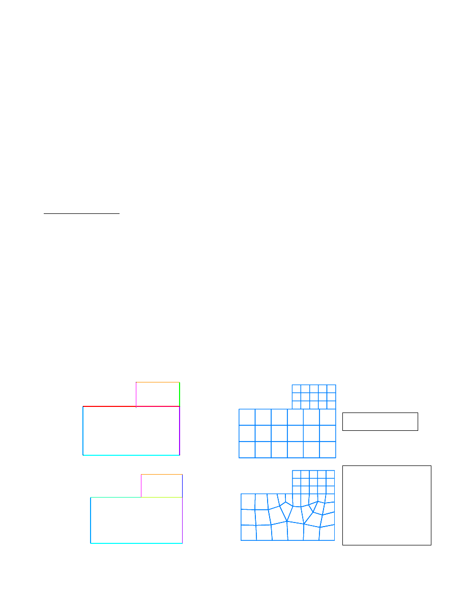
Glue: Take two entities that are touching and make them contiguous or congruent so that when
meshed they will share common nodes. For example, using default mesh parameters,
L1
L2
L4
L5
L6
L7
L8
L1
L2
L4
L5
L6
L7
L8
Area 1
Area 2
L3
L3
Meshing without gluing
areas.
Meshing after gluing areas.
Note: The coincident nodes
on the common line
between the two areas will
be automatically merged.
You don’t have to manually
equivalence them like in
some other codes.
L1
L2
L4
L7
L8
L9
L10
L11
Area 1
Area 2
Copyright 2003 Belcan Engineering Group, Inc.
6
The Working Plane:
All geometry is created with respect to the working plane, which by default is aligned with the global
Cartesian coordinate system. The “Working Plane” is actually the XY plane of the working coordinate
system. The working coordinate system ID is coordinate system 4 in ANSYS. Global Cartesian is ID
0, Global Cylindrical is ID 1, and Global Spherical is ID 2.
Working Plane Hints:
Turn on the working plane so you can see it with, “Utility Menu
→ Work Plane →
Display Working Plane”.
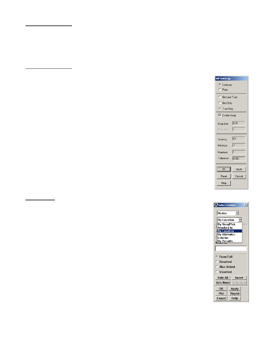
Change the way the working plane looks or adjust the snap settings under “Utility
Menu
→ Work Plane → WP Settings…”.
Move the working plane around using “Utility Menu
→ Work Plane → Offset WP
to…”.
Align the working plane with various parts of the model using “Utility Menu
→ Work
Plane
→ Align WP with…”.
If you select more than one node or keypoint to offset the working plane to, it will go
to the average location of the selected entities. VERY handy!
Use the working plane to slice and dice your model. For example to cut an area in
pieces use “Main Menu
→ Modeling → Operate → Booleans → Divide → Area by
WrkPlane”. Do this for lines and volumes as well.
Select Logic:
Selecting is an important and fundamental concept in ANSYS. Selected entities are
your active entities. All operations (including Solving) are performed on the selected
set. In many operations you select items “on the fly”; ANSYS prompts for what
volumes to mesh for example, you pick them with the mouse, and ANSYS does the
meshing. However there are many times when you need to select things in more
sophisticated ways. Also, in an ANSYS input file or batch file you can’t select things
with the mouse!
Examples where this would be useful:
• You have many different areas at Z = 0 you want to constrain. You could select
them all one by one when applying the constraint, or select “By Location”
beforehand, then say “Pick All” in the picking dialog.
• You have a structure with many fastener holes that you want to constrain. Again,
you could select them all one by one when applying the constraint, or select lines
“By Length/Radius”, type in the radius of the holes to select all of them in one shot, then “Pick
All” in the picking dialog when applying the constraint.
Copyright 2003 Belcan Engineering Group, Inc.
7
After working with the selected set, “Utility Menu
→ Select → Everything” to make the whole model
active again.
Select Entities Dialog Box Terminology:
From Full: Select from the entire set of entities in the model.
Reselect: Select a subset from the currently selected entities.
Also Select: Select in addition to (from the whole model) the set you have currently selected.
Unselect: Remove items from the selection set.
Select All: This is not the same as “Utility Menu
→ Select → Everything”. This selects all of
whatever entity you have specified at the top of the dialog.
Invert: Reverses the selected and unselected entities (just the entities specified at the top of the
dialog).
OK: This does the select operation (or brings up a picker dialog so that you can pick with the mouse)
and then dismisses the dialog.
Apply: This does the operation but keeps the dialog box. Typically use this so the dialog stays active.
Replot: Replots whatever is active in the graphics window.
Plot: Plots only the entity specified at the top of the dialog.
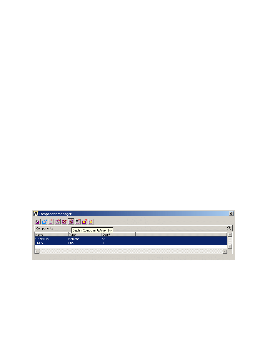
Organizing Your Model Using Components:
If you select a group of entities and think that you might want to use that selection set again, create a
component out of it. Components are groups of entities but hold only one kind of entity at a time.
Components can themselves be grouped into Assemblies, so this is how you group different types of
entities together. Use “Utility Menu
→ Select → Comp/Assembly → Create Component…” to create
a component. The new Component Manager in Release 8.0 makes it very easy to manage and
manipulate groups and select/plot what you want to see to the screen. This is found under “Utility
Menu
→ Select → Component Manager”.
Copyright 2003 Belcan Engineering Group, Inc.
8
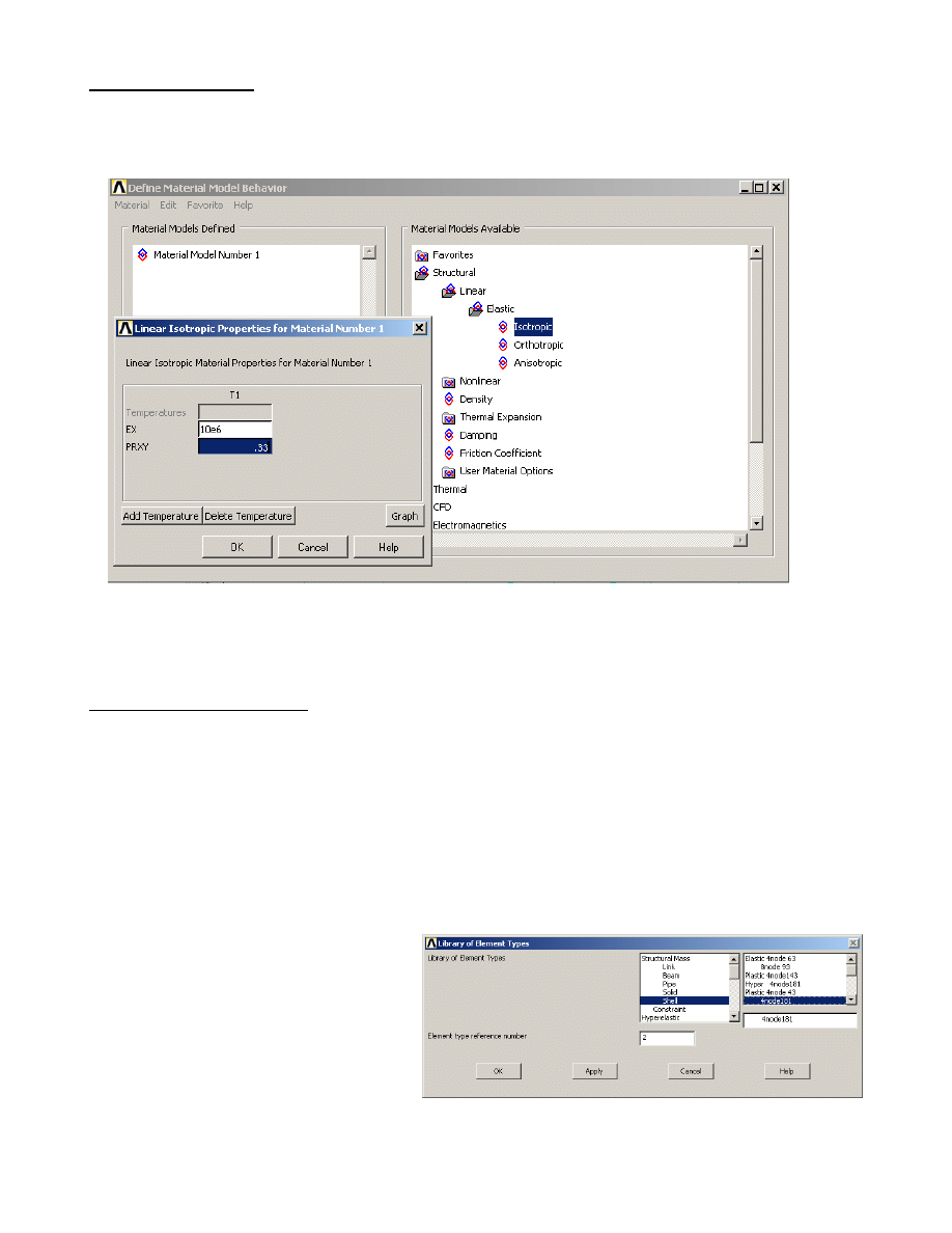
Creating a Material:
Create the material properties for your model in “Main Menu
→ Preprocessor → Material Props →
Material Models”. This gives you this dialog box where all materials can be created,
Double click on items in the right hand pane of this window to get to the type of material model you
want to create. All properties can be temperature dependant. Click OK to create the material and it
will appear in the left hand pane. Create as many different materials as you need for your analysis.
Selecting an Element Type:
ANSYS has a large library of element types. Why so many? Elements are organized into groups of
similar characteristics. These group names make up the first part of the element name (BEAM,
SOLID, SHELL, etc). The second part of the element name is a number that is more or less (but not
exactly) chronological. As elements have been created over the past 30 years the element numbers
have simply been incremented. The earliest and simplest elements have the lowest numbers (LINK1,
BEAM3, etc), the more recently developed ones have higher numbers. The “18x” series of elements
(SHELL181, SOLID187, etc) are the newest and most modern in the ANSYS element library.
Tell ANSYS what elements you are going to use in your model using “Main Menu
→ Element Type
→ Add/Edit/Delete”.
Later, when meshing or creating elements
manually you will need to tell ANSYS
what type of elements you want to create.
See the Belcan “ANSYS Tips” sheet
called “Common Element Types for
Structural Analysis” for more information.
Copyright 2003 Belcan Engineering Group, Inc.
9
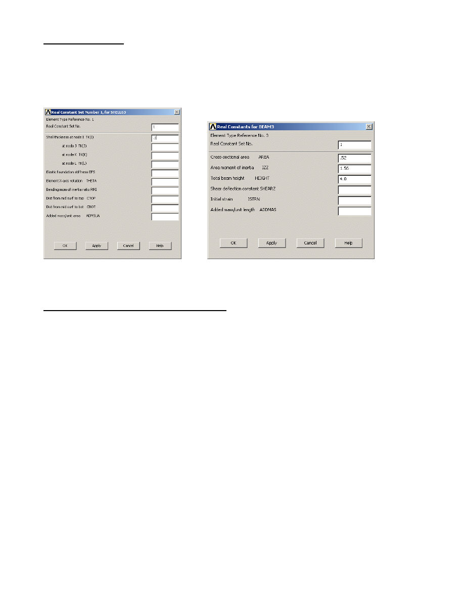
Creating Properties:
solid element (brick or tet) knows its thickness, length, volume, etc by virtue of its geometry, since it
A
is defined in 3D space. Shell, beam and link (truss) elements do not know this information since they
are a geometric idealization or engineering abstraction. Properties in ANSYS are called Real
Constants. Define real constants using “Main Menu
→ Real Constants → Add/Edit/Delete”.
ater when meshing or creating elements manually ANSYS will need to know what real constant set
reating the Finite Elements Model - Meshing:
L
you want to use for those elements.
C
you are just starting out in FEA, it is important to realize that your geometry (called the solid model
all
he
e in
nother very good reason we mesh geometry is that we assign materials and properties to that
on’t
teps for Creating the Finite Elements:
1. Assign Attributes to Geometry (materials, real constants, etc).
nt).
If
in ANSYS) is not your finite element model. In the finite element method we take an arbitrarily
complex domain, impossible to describe fully with a classical equation, and break it down into sm
pieces that we can describe with an equation. These small pieces are called finite elements. We
essentially sum up the response of all these little pieces into the response of our entire structure. T
solver works with the elements. The geometry we create is simply a vehicle used to tell ANSYS
where we want our nodes and elements to go. While you can create nodes and elements one by on
a manual fashion (called direct generation in ANSYS) most people mesh geometry because it is much
faster.
A
geometry. Then any element created on or in that geometric entity gets those attributes. If we d
like the mesh we can clear it and re-mesh, without having to re-assign the attributes.
S
2. Specify Mesh Controls on the Geometry (element sizes you wa
3. Mesh.
Copyright 2003 Belcan Engineering Group, Inc.
10
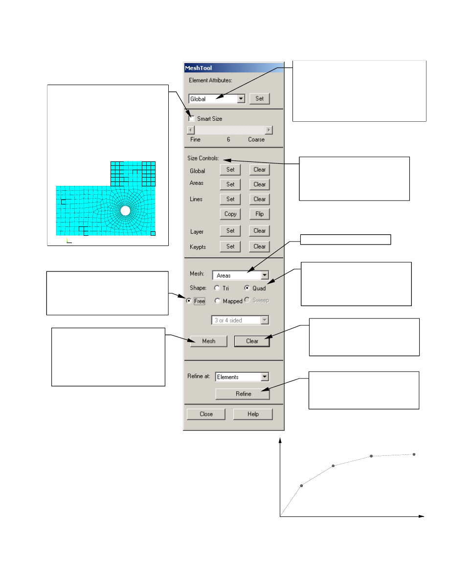
Most of the meshing operations can be done within the MeshTool, so that will be examined in some
detail now. Start it from “Main Menu
→ Preprocessor → Meshing → MeshTool”.
Refine the mesh (make more nodes
and elements locally) at a specific
location (elements, nodes, kepoints,
lines,etc.).
Brings up a picker dialog. You pick
the entities to be cleared, press OK,
and ANSYS removes the nodes and
elements from that geometry.
Brings up a picker dialog. Pick the
entities to be meshed (or Pick All if
you have made some selection using
select logic), press OK, and ANSYS
generates the nodes and elements
on/in that geometry.
A mapped mesh generates a very regular
grid of elements. This can only be used
on rectangular shaped areas or volumes.
A free mesh will mesh any entity -
regardless of shape.
If you want to set a specific element
edge length on an entity or tell
ANSYS to put some specific
number of elements along a line for
example, use this.
Shape of the element you want to
create. For Volumes you would
have the choice of Hex or Tet. You
can create beam elements by
meshing lines.
Pick what you want to mesh.
Smart Size is used to automatically pick
the element edge length depending on
the sizes of features in the geometry. It
makes a finer mesh around smaller
features in order to capture them
adequately. For example in the mesh
below no sizes were specified at all
except a Smart Size level of 4.
X
Y
Z
If you set global attributes, that material,
element type, real constant, beam section,
etc. will be used for all elements in the
model. It’s better to use the drop down to
assign different attributes to different
geometric entities in the model. Then mesh
the whole model at one time.
How fine of a mesh should you have? Part of this is
common sense. Put a finer mesh in areas of higher
stress gradient, like near a stress concentration. Do
simple experiments along with hand calculations; for
example I know I need about 30 nodes around a hole to
get a good value of the peak stress. Your stress
convergence should follow a pattern as shown at right.
When the result is not changing much for a finer mesh,
you have mesh convergence.
number of nodes in the model
stress
at
some
point
in the
model
you care
about
Copyright 2003 Belcan Engineering Group, Inc.
11

Applying Loads and Boundary Conditions:
Loads and boundary conditions can be applied in both the Preprocessor (“Main Menu
→ Preprocessor
→ Loads → Define Loads → Apply”), and the Solution processor (“Main Menu → Solution → Define
Loads
→ Apply”).
1. Select the kind of constraint you want to apply.
2. Select the geometric entity where you want it applied.
3. Enter the value and direction for it.
There is no “modify” command for loads and B.C.’s. If you make a mistake simply apply it again with
a new value (the old one will be replaced if it’s on the same entity), or delete it and reapply it.
Loads: Forces, pressures, moments, heat flows, heat fluxes, etc.
Constraints: Fixities, enforced displacements, symmetry and anti-symmetry conditions, temperatures,
convections, etc.
Although you can apply loads and boundary conditions to nodes or elements, it’s generally better to
apply all B.C.’s to your geometry. When the solve command is issued, they will be automatically
transferred to the underlying nodes and elements. If B.C.’s are put on the geometry, you can re-mesh
that geometry without having to reapply them.
Solving:
Solution is the term given to the actual simultaneous equation solving of the mathematical model. The
details of how this is done internally is beyond the scope of this guideline but is addressed in a separate
“ANSYS Tips” white paper. For the moment, it is sufficient to say that the basic equation of the finite
element method that we are solving is,
[ ]{ } { }
K u
F
=
, where [K] is the assembled stiffness matrix of
the structure, {u} is the vector of displacements at each node, and {F} is the applied load vector. This
is analogous to a simple spring and is the essence of small deflection theory.
To submit your model to ANSYS for solving, go to “Main Menu
→ Solution → Solve → Current LS”.
LS stands for load step. A load step is a loading “condition”. This is a single set of defined loads and
boundary conditions (And their associated solution results. More on this in the next section). Within
an interactive session the first solve you do is load step 1, the next solution is load step 2, etc. If you
leave the solution processor after solving to do post-processing for example, the load step counter gets
set back to one. You can also define and solve multiple load steps all at once.
There are several solvers in ANSYS that differ in the way that the system of equations is solved for the
unknown displacements. The two main solvers are the sparse solver and the PCG solver. If the choice
of solvers is left to “program chosen” then generally ANSYS will use the sparse solver. The PCG
(preconditioned conjugate gradient) solver works well for models using all solid elements. From a
practical perspective one thing to consider is that the sparse solver doesn’t require a lot of RAM but
swaps out to the disk a lot. Disk I/O is very slow. If you have a solid model and lots of RAM the PCG
solver could be significantly faster since the solution runs mostly in core memory.
Copyright 2003 Belcan Engineering Group, Inc.
12
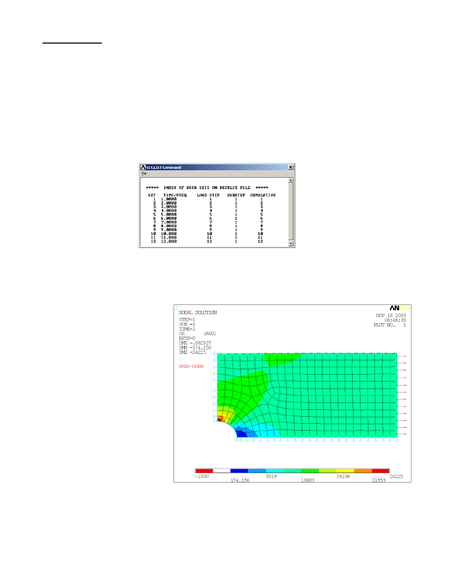
Postprocessing:
The General Postprocessor is used to look at the results over the whole model at one point in time.
This is the final objective of everything we have discussed so far; finding the stresses, deflections,
temperature distributions, pressures, etc. These results can then be compared to some criteria to make
an objective evaluation of the performance of your design.
The solution results will be stored in the results file as result “sets”. For a linear static analysis like we
are talking about, the correlation between Load Step numbers and Results Set numbers will be one to
one as shown below. Only one set of results can be stored in the database at a time, so when you want
to look at a particular set, you have to read it in from the results file. Reading it in clears the previous
results set from active memory.
To read in a results set from the results file (not needed if you have run only a single load step) use
“Main Menu
→ General Postproc → Read Results → First Set, or By Pick”. Most results are
displayed as a contour plot as shown below. To generate a plot of stresses use “Main Menu
→ General
Postproc
→ Plot Results → Contour Plot → Nodal Solution”, then pick the stresses you want to see.
There are many, many other ways
to look at your results data
including:
• Listing them to a file.
• Querying with the mouse to
find a result at a particular
node.
• Graphing results along a path.
• Combining different load
cases.
• Summing forces at a point.
• Extracting data and storing it an APDL array that you can do further operations with.
Animate any result on the deformed shape with “Utility Menu
→ Plot Ctrls → Animate”. This is very
helpful for understanding if your model is behaving in a reasonable way.
Copyright 2003 Belcan Engineering Group, Inc.
13
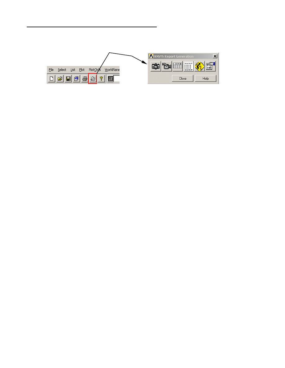
Documenting your Analysis and Outputting Graphics:
ANSYS has a Report Generator available from the main toolbar, which can help you put together an
HTML report by capturing images, window listings, etc.
To print a hardcopy of the graphics window: “Utility Menu
→ Plot Ctrls → Hard Copy → To Printer”
There are several ways of capturing a graphic image for use in Microsoft Word, Powerpoint or some
other software.
Exact screen shot of the graphics window: “Utility Menu
→ Plot Ctrls → Capture Image” will pop up
another window with a screen shot of your graphics window. You can keep it available for later
reference or save the image to a bitmap (.bmp) file. Note that although a windows bitmap file is not
compressed, when it is inserted into Word it does get compressed automatically so you don’t end up
with a huge bloated document.
Output a vector image: “Utility Menu
→ Plot Ctrls → Redirect Plots → To PSCR File…”. A
Postscript file is a vector file, which means that it is a 2D representation of all of the entities in the
graphics window in an editable format. Because it is not a bitmap, it can be scaled to any size without
losing any resolution, and is always very crisp looking. It can also be imported into a technical
illustration program and manipulated very easily: change the colors, add annotations, change or resize
fonts, etc. All this can be done in ANSYS but it can be quicker in an illustration package. One caution
about Postscript files! Since they actually write out every entity in the model, if your model is large
(say a tet mesh of a CAD model) this file can be huge. It is best suited for getting very crisp images of
smallish models or wireframe displays. Microsoft Word will not display the image until it is printed.
A very good free program to look at and manipulate Postscript files with (available on the web) is
called “GSView”.
Output a bitmap image: “Utility Menu
→ Plot Ctrls → Redirect Plots → To xyz File…”, where xyz is
JPEG, TIFF, PNG, etc. These file formats produce good images with reasonably small file sizes. The
size of the image file for these formats is not dependant on the size of your model like Postscript.
Note: The GRPH format is the ANSYS native image format. You can only deal with these files using
the ANSYS DISPLAY program that is available from “Start Menu
→ Programs → ANSYS 8.0 →
Display”. This utility has some neat features like being able to take a group of static images you create
and animating them into an mpeg or avi video.
Copyright 2003 Belcan Engineering Group, Inc.
14
Controlling the Way Your Model Looks:
All of the visual aspects of what you see in the graphics window are controlled from the “Plot” and
“Plot Ctrls” pull downs from the Utility menu. Use “Utility Menu
→ Plot” to plot different types of
entities to the screen. Use “Utility Menu
→ Plot Ctrls” to control the characteristics of what you are
plotting.
“Utility Menu
→ Plot Ctrls → Numbering”: Entity Numbers on and off.
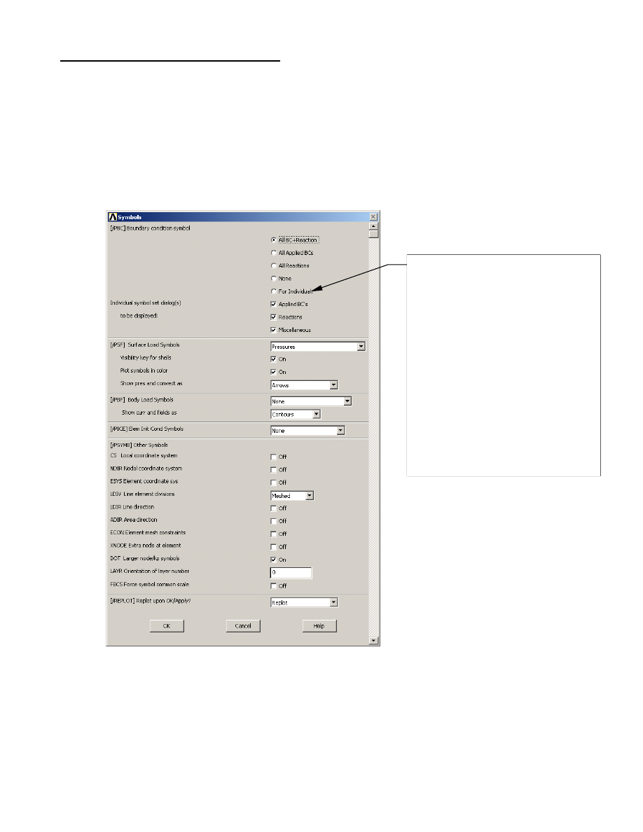
“Utility Menu
→ Plot Ctrls → Symbols”: Turn various markers and symbols on and off.
This is the most important button in this
dialog, because it is not intuitive what this
does. If you pick this and then click “OK” at
the bottom of this window, you will get three
subsequent dialogs where you can turn the
individual symbols on and off, as well as
their values (the “All” buttons above it will
not show you the values, only the symbols).
This is very commonly used to display just
the force vectors along with their values on
the model for documentation purposes (for
example). Under “Reactions” you can turn
on the reaction vectors and their values as
well as “free-body” type forces. That is to
say, the balancing forces acting on a node
due to other elements attached to it but not
selected.
“Utility Menu
→ Plot Ctrls → Style”: Change hidden line, element edges, element shrink, etc.
“Utility Menu
→ Plot Ctrls → Device Options”: Change between solid shaded and wireframe display.
Copyright 2003 Belcan Engineering Group, Inc.
15
ANSYS Parametric Design Language and Macros:
APDL is the command language that drives ANSYS. Every GUI selection has a command equivalent
that is executed when you click Apply or OK. All commands are well documented and if you know
them you can type them in the command window instead of making a GUI selection. This can be
faster than the mouse, but the real power of ANSYS is in easily automating tasks by stacking these
commands into a text file and reading the file in to execute the commands all at once.
Basic APDL commands are all laid out simply and in the same fashion,
CommandName, argument1, argument2, argument3, argument4, etc.
How do you know what the command equivalent is of a GUI operation?
1. Use the
jobname.log
file. A record of all your actions in ANSYS is kept here in the form of
commands. Do an operation in the GUI, then open up that file and look at the last line to see
the command used.
2. All GUI operations also give a hint to the command name, either in the dialog box itself or in
the hint line. It’s always given in square brackets. In the command window enter
help,commandName
to bring up detailed help for that command that describes what each
argument is.
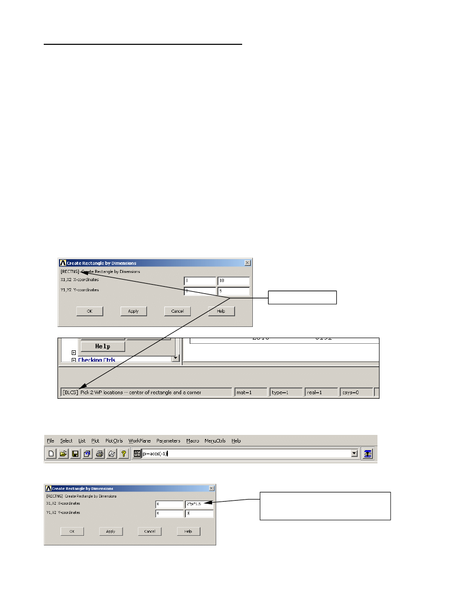
[command name]
Define parameter variables to use in your analysis with “Utility Menu
→ Scalar Parameters”. Or just
type in a variable using the equals sign in the command window. For example:
Now you could refer to this variable in a dialog box and ANSYS will substitute the value of “pi”.
Use parameters and mathematical
expressions in any entry box that requires
a number. Handy!
Copyright 2003 Belcan Engineering Group, Inc.
16

APDL has much of the functionality of a full-featured programming language including mathematical
functions and branching logic. Macros are APDL commands put into a file with a
.mac
extension.
ANSYS will use these macros just like a regular ANSYS command. Here’s a simple example, called
edges.mac
:
C*** Reverses current display of all element edges
C*** (if edges on, turns them off & vice versa)
*GET,KEY,GRAPH,1,EDGE
! obtains current setting using a “*get” command
*IF,KEY,EQ,0,THEN
/EDGE,1,1
! sets KEY=1
*ELSE
/EDGE,1,0
! sets KEY=0
*ENDIF
/REPLOT
In the command line simply type: edges ↵ to execute the macro. (note: ↵ ≡ press ENTER)
An analysis (building the model, solving, and postprocessing) can be completely defined using APDL
commands and this does have some excellent benefits such as,
• Your analysis is completely documented by your input file (you can add user comments as well).
• You can use parameter variables to define dimensions or loading and have a parametric input file
that you can run as many times as you want, changing the model each time by changing the
variable values.
Customizing the GUI:
Another productivity enhancement that goes right along with APDL macros is customizing the
abbreviation toolbar. Any ANSYS command or macro can be assigned to a toolbar button using the
*ABBR
command or “Utility Menu
→ MenuCtrls → Edit Toolbar”. The format of the command is:
*ABBR, name on the button, command
Some examples of abbreviation button commands,
*ABBR,WP-KP,KWPAVE,P
! move the working plane to avg of keyoints
*ABBR,STR_LINE,L,P
! create a line between two points
As you can see, the possibilities for customization of the toolbar to enhance productivity are limitless.
To customize the location where dialog boxes pop up, arrange them how you want them to be the next
time they appear, use “Utility Menu
→ MenuCtrls → Save Menu Layout”. This saves the locations.
Grab any of the solid bars that divide the main window panes and drag them to resize. The main
graphics window does have a fixed aspect ratio however; you will notice this as you try to change it to
a wide thin window for example.
Copyright 2003 Belcan Engineering Group, Inc.
17
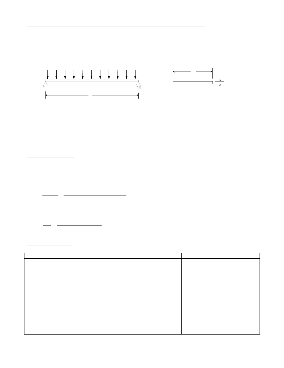
Example - An Analysis of a Simply Supported Beam Using Three Methods:
To demonstrate the general flow of an ANSYS simulation we will show an analysis of a simply
supported beam under uniform pressure, analyzed with beam elements, shell elements, and solid
elements. These results will be compared with a hand calculation which is also a good idea to confirm
the results are reasonable.
p
L
beam section
W
t
Input data needed for this analysis:
L = 12 in.
W = 2 in.
t = 0.125 in.
p = 1.0 psi
E = 10 e 6 psi
ν = 0.33
The running load for the beam model will be (1.0 psi)(2
″ wide) = 2.0 lb/in
Theoretical Solution:
( )(
)
4
3
3
in
000326
.
0
5
12
.
0
0
.
2
12
1
t
b
12
1
I
=
′′
′′
=
=
(
)( )( )
lbs
in
36
8
2
1
0
.
2
psi
0
.
1
8
L
b
p
M
2
2
⋅
=
′′
′′
=
=
(
)( )( )
(
)
(
)
in
055296
.
0
in
000326
.
0
psi
6
e
30
384
2
1
0
.
2
psi
0
.
1
5
I
E
384
L
b
p
5
4
3
2
max
=
′′
′′
=
=
δ
(
)
psi
6912
in
000326
.
0
2
5
12
.
0
lbs
in
36
I
Mc
4
max
=
′′
⋅
=
=
σ
ANSYS Instructions:
Beam Element Model
Shell Element Model
Solid Element Model
Start
→ Programs → ANSYS 8.0 →
Configure ANSYS Products. This
starts the ANSYS Launcher.
Click the File Management tab, select
your working directory and change the
jobname to beam1.
Click Run in the Launcher to start
ANSYS.
Main Menu
→ Preferences →
Structural. This filters out all
disciplines except structural.
Start
→ Programs → ANSYS 8.0 →
Configure ANSYS Products. This
starts the ANSYS Launcher.
Click the File Management tab, select
your working directory and change the
jobname to beam2.
Click Run in the Launcher to start
ANSYS.
Main Menu
→ Preferences →
Structural. This filters out all
disciplines except structural.
Copyright 2003 Belcan Engineering Group, Inc.
18
Beam Element Model
Shell Element Model
Solid Element Model
Main Menu
→ Preprocessor →
Element Type
→ Add/Edit/Delete. The
first thing we do is tell ANSYS what
kind of element we will be using for
the analysis.
In the Element Types dialog click Add
→ Beam → 3 node 189 → OK →
Close.
Create the material. Main Menu
→
Preprocessor
→ Material Props →
Material Models. Double click
Structural
→ Linear → Elastic →
Isotropic. Enter the values for the
modulus (30e6) and Poisson’s ratio
(0.33)
→ OK → Material → Exit.
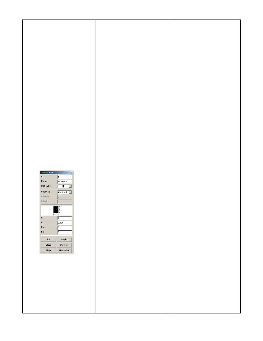
Create a beam section with the Beam
Tool so that the real constants
(properties) for the beam are
automatically calculated and applied.
Main Menu
→ Preprocessor →
Sections
→ Beam Common Sections.
Fill out the form with the name of
“example” for the section and B = 2
and H = 0.125
→ Preview → OK.
Create keypoints; one for each end of
the beam and one reference keypoint
that will be used to tell ANSYS what
the orientation of our beam is. Main
Menu
→ Preprocessor → Modeling →
Create
→ Keypoints → In Active CS.
Create points at {0,0,0}
→ Apply,
{12,0,0}
→ Apply, and {0,1,0} → OK.
Create a line to represent the beam.
Main Menu
→ Preprocessor →
Element Type
→ Add/Edit/Delete. The
first thing we do is tell ANSYS what
kind of element we will be using for
the analysis.
In the Element Types dialog click Add
→ Shell→ 4noded181 → OK →
Close.
Create the Real Constant that will
define the thickness of the shell
elements. Main Menu
→ Preprocessor
→ Add/Edit/Delete → Add →
SHELL181
→ OK → Enter 0.125 for
the thickness at Node I
→ OK →
Close.
Create the material. Main Menu
→
Preprocessor
→ Material Props →
Material Models. Double click
Structural
→ Linear → Elastic →
Isotropic. Enter the values for the
modulus (30e6) and Poisson’s ratio
(0.33)
→ OK → Material → Exit.
Create a rectangular area to represent
the beam. Main Menu
→Preprocessor
→ Modeling → Create → Areas →
Rectangle
→ By Dimensions → {0,0}
and {12,2}
→ OK.
Start the MeshTool. Main Menu
→
Preprocessor
→ Meshing →
MeshTool.
Assign element attributes to the area.
From the top of the MeshTool under
element attributes pick Areas and then
Set. Pick the area and then OK in the
picker dialog. For this simple model
with only one real, material, etc, we
can accept the defaults and click OK.
Assign element sizes to the area before
meshing it. From Size Controls
section of the MeshTool pick Areas
Set. Pick the area and then OK in the
picker dialog. Enter 0.5 for the
Element Edge Length, OK.
Create the shell elements on the area.
From the MeshTool in the Mesh
section, Mapped
→ Mesh Button →
Pick the area
→ OK in the picker.
Main Menu
→ Preprocessor →
Element Type
→ Add/Edit/Delete. The
first thing we do is tell ANSYS what
kind of element we will be using for
the analysis.
In the Element Types dialog click Add
→ Solid → 20Node 186 → OK →
Close.
Create the material. Main Menu
→
Preprocessor
→ Material Props →
Material Models. Double click
Structural
→ Linear → Elastic →
Isotropic. Enter the values for the
modulus (30e6) and Poisson’s ratio
(0.33)
→ OK → Material → Exit.
Create a solid block to represent the
beam. Main Menu
→ Preprocessor →
Modeling
→ Create → Volumes →
Block
→ By Dimensions → {0,0,0}
and {12,2,0.125}
→ OK.
Start the MeshTool. Main Menu
→
Preprocessor
→ Meshing →
MeshTool.
Assign element attributes to the
volume. From the top of the MeshTool
under element attributes pick Volumes
and then Set. Pick the block and then
OK in the picker dialog. For this
simple model with only one material,
etc, we can accept the defaults and
click OK.
Assign element sizes to the area before
meshing it. From Size Controls
section of the MeshTool pick Global
Set. Pick the block and then OK in the
picker dialog. Enter 0.25 for the
Element Edge Length, OK.
Create the brick elements in the
volume. From the MeshTool in the
Mesh section, Volumes
→ Hex →
Mapped
→ Mesh Button → Pick the
volume
→ OK in the picker.
Use the Control key and the right
mouse button to rotate the model such
that the global Z-axis is pointing up for
a better view.
Copyright 2003 Belcan Engineering Group, Inc.
19
Beam Element Model
Shell Element Model
Solid Element Model
Main Menu
→ Preprocessor →
Modeling
→ Create → Lines → Lines
→ Straight Lines. Pick the end points
of the line (keypoints 1 & 2), OK.
Turn on the keypoint numbers. Utility
Menu
→PlotCntrls → Numbering →
Keypoints.
Plot the lines and keypoints to the
screen. Utility Menu
→ Plot →
Multiplot.
Start the MeshTool. Main Menu
→
Preprocessor
→ Meshing →
MeshTool.
Tell ANSYS what attributes to mesh
the line with. At the top of the
MeshTool under “Element Attributes”
select Lines from the drop down
→
Set. Pick the line and OK in the
picking dialog. Since we have only
one property we can accept all defaults
except click the “Pick Orientation
Keypoint(s)” checkbox to Yes
→ OK.
Pick keypoint 3 as the orientation
keypoint.
Assign element sizes to the line before
meshing it. From Size Controls
section of the MeshTool pick Lines
Set. Pick the line and then OK in the
picker dialog. Enter 1.0 for the
Element Edge Length, OK.
Create the beam elements on the line.
From the MeshTool, Mesh
→ Pick the
line
→ OK in the picker.
Change to an Oblique view. From the
View toolbar on the RHS of the
graphics window click
.
Display the beam section on the line.
Utility Menu
→ PlotCntrls → Style →
Size and Shape
→ Turn on “Display of
Element Shapes”
→ OK.
Apply constraints to the ends of the
beam. Main Menu
→ Solution →
Apply
→ Structural → Displacement
→ On Keypoints → Pick the end
keypoints of the line
→ OK in the
picker
→ click on UX, UY, UZ, and
ROTX
→ OK.
Use the Control key and the right
mouse button to rotate the model such
that the global Z-axis is pointing up for
a better view.
Display the shell thickness. Utility
Menu
→ PlotCntrls → Style → Size
and Shape
→ Turn on “Display of
Element Shapes”
→ OK.
Apply simple support constraints to the
ends of the beam. Main Menu
→
Solution
→ Apply → Structural →
Displacement
→ On Lines → Pick the
short lines at the ends of the area
→
OK in the picker
→ click on UX →
Apply
→ Pick the lines again → OK in
the picker
→ click on UY → Apply →
Pick the lines again
→ OK in the
picker
→ click on UZ → OK.
Apply a pressure to the beam. Main
Menu
→ Solution → Apply →
Structural
→ Pressure → On Areas →
Pick All
→ OK in the picker → Enter
-1.0 for Pressure Value
→ OK.
Utility Menu
→ PlotCntrls → Symbols
→ Surface Load Symbols → Pressures
→ Show pres and convect → Arrows
→ OK. Utility Menu → Plot →
Multiplot, to see the loads and B.C.’s
on the line.
Save the model. Utility Menu
→ File
→ Save Jobname.db.
Solve the model. Main Menu
→
Solution
→ Solve → Current LS.
Review and close the “/STATUS”
window
→ OK in the Solve dialog.
Plot the displacements. Main Menu
→
General Postproc
→ Plot Results
→Contour Plot → Nodal Solution →
DOF Solution
→ USUM → OK.
Max Displacement = 0.0548
″
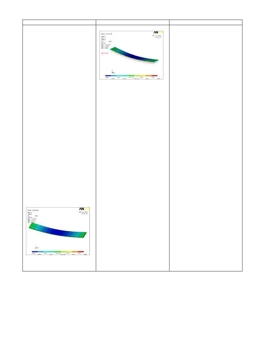
Plot the stresses. Main Menu
→
General Postproc
→ Plot Results
→Contour Plot → Nodal Solution →
Stresses
→ X-direction SX → OK.
Apply simple support constraints to the
ends of the beam. Main Menu
→
Solution
→ Apply → Structural →
Displacement
→ On Lines → Pick the
bottom line at one end of the volume
→
OK in the picker
→ click on All DOF
→ Apply → Pick the bottom line at the
other end of the beam
→ OK in the
picker
→ click on UZ only → OK.
Apply a pressure to the beam. Main
Menu
→ Solution → Apply →
Structural
→ Pressure → On Areas →
Pick the top surface area of the block
→ OK in the picker → Enter 1.0 for
Pressure Value
→ OK.
Utility Menu
→ PlotCntrls → Symbols
→ Surface Load Symbols → Pressures
→ Show pres and convect → Arrows
→ OK. Utility Menu → Plot →
Multiplot, to see the loads and B.C.’s
on the line.
Save the model. Utility Menu
→ File
→ Save Jobname.db.
Solve the model. Main Menu
→
Solution
→ Solve → Current LS.
Review and close the “/STATUS”
window
→ OK in the Solve dialog.
Plot the displacements. Main Menu
→
General Postproc
→ Plot Results
→Contour Plot → Nodal Solution →
DOF Solution
→ USUM → OK.
Max Displacement = 0.0555
″
Plot the stresses. Main Menu
→
General Postproc
→ Plot Results
→Contour Plot → Nodal Solution →
Stresses
→ X-direction SX → OK.
Max Stress = 6931 psi
Copyright 2003 Belcan Engineering Group, Inc.
20
Beam Element Model
Shell Element Model
Solid Element Model
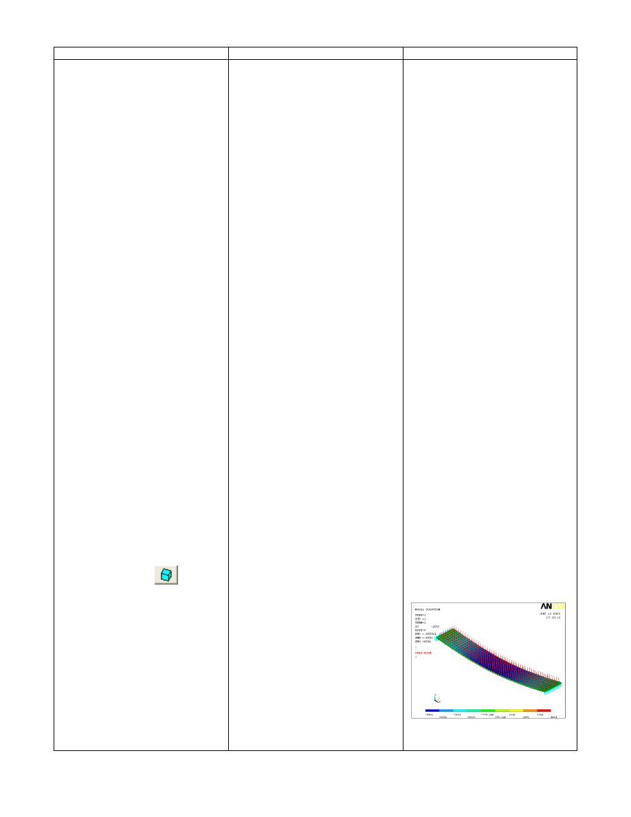
Apply a running load to the top of the
beam. Main Menu
→ Solution →
Apply
→ Structural → Pressure → On
Beams
→ Pick All → OK in the picker
→ Enter 2.0 for Pressure Value →
OK.
Utility Menu
→ PlotCntrls → Symbols
→ Surface Load Symbols → Pressures
→ Show pres and convect → Arrows
→ OK. Utility Menu → Plot →
Multiplot, to see the loads and B.C.’s
on the line.
Save the model. Utility Menu
→ File
→ Save Jobname.db.
Solve the model. Main Menu
→
Solution
→ Solve → Current LS.
Review and close the “/STATUS”
window
→ OK in the Solve dialog.
Plot the displacements. Main Menu
→
General Postproc
→ Plot Results
→Contour Plot → Nodal Solution →
DOF Solution
→ USUM → OK.
Max Displacement = 0.0553
″
Plot the stresses. Main Menu
→
General Postproc
→ Plot Results
→Contour Plot → Nodal Solution →
Stresses
→ X-direction SX → OK.
Max Stress = 6944 psi
Max Stress = 6896 psi
Copyright 2003 Belcan Engineering Group, Inc.
21

Appendix A - Example 1 Analysis APDL Input File:
! ANSYS Quick Start Guide: Beam 1 Example
! Paul Dufour
! Belcan Corporation
! December 2003
finish
/clear
/PREP7
! Enter ANSYS preprocessor
!!!!! PARAMETERS !!!!!!!!!!!!!!!!!!!!!!!!!!!!!!!!!!!!!!!
! To change the model we can simply change these here.
modulus=30e6
poissons=0.33
beam_length=12
beam_width=2
beam_height=0.125
!!!!!!!!!!!!!!!!!!!!!!!!!!!!!!!!!!!!!!!!!!!!!!!!!!!!!!!!
!Define element type to be used: BEAM189, three noded quadratic beam
ET
,1,BEAM189
! Material is steel
MPTEMP
,,,,,,,,
MPTEMP
,1,0
MPDATA
,EX
,1,,modulus
MPDATA
,PRXY
,1,,poissons
! Create the geometric keypoints
K
,,,,,
K
,,beam_length,,,
! This one will be the orientation keypoint
K
,,0,1,,
! Draw the line
LSTR
,1,2
/auto
! fit the view
! Create the beam section
SECTYPE
,1
,BEAM,RECT
,example,0
SECOFFSET
,
CENT
SECDATA
,beam_width,beam_height,0,0,0,0,0,0,0,0
! Assign attributes to the line
LATT
,1,,1,,3,,1
! Sepcify the element sizes
LESIZE
,all
,1.0
! Mesh the line with beam elements
LMESH
,1
/ESHAPE
,1.0
! turn on the beam shape
finish
! exit the preprocessor
/solu
! enter the solution module
! Constrain the ends of the beam
DK
,1,,,,0
,UX,UY,UZ,ROTX
DK
,2,,,,0
,UX,UY,UZ,ROTX
! Apply the running load to the beam elements
Copyright 2003 Belcan Engineering Group, Inc.
22

SFBEAM
,all
,1
,PRES
,2.0
solve
! submit the model to ANSYS for solving
finish
! exit the solution module
/post1
! Enter the general post-processor
! plot the loads and b.c.'s on the model
/PSF
,PRES,NORM
,2,0,1
/PBC
,ALL
,,1
/PBC
,NFOR
,,0
/PBC
,NMOM
,,0
/PBC
,RFOR
,,0
/PBC
,RMOM
,,0
/PBC
,PATH
,,0
! plot the deflection
PLNSOL
,U,SUM
,0,1
! plot the stresses in the beam
PLNSOL
,S,X
,0,1
! store the maximum plotted stress value in a parameter variable
*get
,maxstress
,plnsol
,0
,max
! Oblique view
/VIEW
,1,1,2,3
/ANG
,1
/REP
,FAST
! all done
Copyright 2003 Belcan Engineering Group, Inc.
23

Appendix B – ANSYS and General FEA References:
1. Moaveni, S., “Finite Element Analysis: Theory and Applications with ANSYS”, 2
nd
Edition,
Prentice Hall, 2003.
2. Lawrence, K.L., “ANSYS Tutorial (Release 7.0)”, Schroff Development Corp. Publications,
2002.
3. Adams, V., and Askenazi, A., “Building Better Products with Finite Element Analysis”,
Onward Press, Sante Fe, NM, 1999.
4. Cook, R.D., Malkus, D.S., and Plesha, M.E., “Concepts and Applications of Finite Element
Analysis”, 3
rd
Edition, John Wiley and Sons, New York, 1989.
5. Segerlind, L.J., “Applied Finite Element Analysis”, John Wiley and Sons, New York, 1976.
6. Smith, I.M., and Griffiths, D.V., “Programming the Finite Element Method”, 2
nd
Edition, John
Wiley and Sons, New York, 1988. (This edition uses FORTRAN77 in its examples.)
7. Smith, I.M., and Griffiths, D.V., “Programming the Finite Element Method”, 3
nd
Edition, John
Wiley and Sons, New York, 1997. (This edition uses Fortran 90 in its examples.)
8. Zienkiewicz, O.C., “The Finite Element Method”, 3
rd
Edition, McGraw-Hill Book Company
Limited, London, 1977.
9. Bathe, K.J., “Finite Element Procedures”, Prentice Hall, 1996.
Copyright 2003 Belcan Engineering Group, Inc.
24

Copyright 2003 Belcan Engineering Group, Inc.
25
Appendix C – ANSYS and General FEA Web Sites:
ANSYS Information
ANSYS Web Site - ANSYS Inc. Home Page. General information regarding the always growing
ANSYS family of products. (www.ansys.com)
ANSYS.net - More commonly know as "Sheldons Site". ANSYS Macro & Info Repository by
Sheldon Imaoka. The best ANSYS site on the web. Huge collection of ANSYS stuff with
contributions by users all over the world. Great! (www.ansys.net/ansys)
ANSYS Tips Page - Many ANSYS pointers and a ton of FEA links, some related to ANSYS and some
general. By Peter Budgell. Hasn't been updated in a few years but most info is still very applicable to
ANSYS currently. (www3.sympatico.ca/peter_budgell/home.html)
ANSYS Tutorials - From the University of Alberta, Canada. This is a very well done and complete set
of tutorials categorized from basic to advanced. (www.mece.ualberta.ca/tutorials/ansys/index.html)
XANSYS.org - Home of the XANSYS list. This is a mailing list of ANSYS users from around the
world with 2500+ members. (www.xansys.org)
General Finite Element Analysis
Finite Element Modeling Continuous Improvement - Site at NASA Goddard Space Flight Center.
(analyst.gsfc.nasa.gov/FEMCI/femci.html)
NAFEMS - A European Engineering Analysis Organization. The "Analysis Resources" section has a
lot of good info and links. (www.nafems.org)
FEA Links Page - many links to finite element resources. Updated in 2003.
(www.engr.usask.ca/%7Emacphed/finite/fe_resources/fe_resources.html)
FEMur - Finite Element Method Universal Resource at WPI (Worcester Polytechnic Institute)
(femur.wpi.edu)
Introduction to FEA by Dermot Monaghan - Although a couple parts are under construction, this guy
has put together a really nice FEA site here. (www.dermotmonaghan.com)
Wyszukiwarka
Podobne podstrony:
więcej podobnych podstron