
Edward Neuman
Department of Mathematics
Southern Illinois University at Carbondale
edneuman@siu.edu
This tutorial is devoted to discussion of the computational methods used in numerical linear
algebra. Topics discussed include, matrix multiplication, matrix transformations, numerical
methods for solving systems of linear equations, the linear least squares, orthogonality, singular
value decomposition, the matrix eigenvalue problem, and computations with sparse matrices.
The following MATLAB functions will be used in this tutorial.
Function
Description
abs
Absolute value
chol
Cholesky factorization
cond
Condition number
det
Determinant
diag
Diagonal matrices and diagonals of a matrix
diff
Difference and approximate derivative
eps
Floating point relative accuracy
eye
Identity matrix
fliplr
Flip matrix in left/right direction
flipud
Flip matrix in up/down direction
flops
Floating point operation count
full
Convert sparse matrix to full matrix
funm
Evaluate general matrix function
hess
Hessenberg form
hilb
Hilbert matrix
imag
Complex imaginary part
inv
Matrix inverse
length
Length of vector
lu
LU factorization
max
Largest component

2
min
Smallest component
norm
Matrix or vector norm
ones
Ones array
pascal
Pascal matrix
pinv
Pseudoinverse
qr
Orthogonal-triangular decomposition
rand
Uniformly distributed random numbers
randn
Normally distributed random numbers
rank
Matrix rank
real
Complex real part
repmat
Replicate and tile an array
schur
Schur decomposition
sign
Signum function
size
Size of matrix
sqrt
Square root
sum
Sum of elements
svd
Singular value decomposition
tic
Start a stopwatch timer
toc
Read the stopwach timer
trace
Sum of diagonal entries
tril
Extract lower triangular part
triu
Extract upper triangular part
zeros
Zeros array
! "#"$
Computation of the product of two or more matrices is one of the basic operations in the
numerical linear algebra. Number of flops needed for computing a product of two matrices
A
and
B
can be decreased drastically if a special structure of matrices
A
and
B
is utilized properly. For
instance, if both
A
and
B
are upper (lower) triangular, then the product of
A
and
B
is an upper
(lower) triangular matrix.
function
C = prod2t(A, B)
% Product C = A*B of two upper triangular matrices A and B.
[m,n] = size(A);
[u,v] = size(B);
if
(m ~= n) | (u ~= v)
error(
'Matrices must be square'
)
end
if
n ~= u
error(
'Inner dimensions must agree'
)
end
C = zeros(n);
for
i=1:n
for
j=i:n
C(i,j) = A(i,i:j)*B(i:j,j);
end
end

3
In the following example a product of two random triangular matrices is computed using function
prod2t
. Number of flops is also determined.
A = triu(randn(4)); B = triu(rand(4));
flops(0)
C = prod2t(A, B)
nflps = flops
C =
-0.4110 -1.2593 -0.6637 -1.4261
0 0.9076 0.6371 1.7957
0 0 -0.1149 -0.0882
0 0 0 0.0462
nflps =
36
For comparison, using MATLAB's "general purpose" matrix multiplication operator
*
,
the number of flops needed for computing the product of matrices
A
and
B
is
flops(0)
A*B;
flops
ans =
128
Product of two Hessenberg matrices
A
and
B
, where
A
is a lower Hessenberg and
B
is an upper
Hessenberg can be computed using function
Hessprod
.
function
C = Hessprod(A, B)
% Product C = A*B, where A and B are the lower and
% upper Hessenberg matrices, respectively.
[m, n] = size(A);
C = zeros(n);
for
i=1:n
for
j=1:n
if
( j<n )
l = min(i,j)+1;
else
l = n;
end
C(i,j) = A(i,1:l)*B(1:l,j);
end
end
We will run this function on Hessenberg matrices obtained from the Hilbert matrix
H
H = hilb(10);

4
A = tril(H,1); B = triu(H,-1);
flops(0)
C = Hessprod(A,B);
nflps = flops
nflps =
1039
Using the multiplication operator
*
the number of flops used for the same problem is
flops(0)
C = A*B;
nflps = flops
nflps =
2000
For more algorithms for computing the matrix-matrix products see the subsequent sections of this
tutorial.
%
"
The goal of this section is to discuss important matrix transformations that are used in numerical
linear algebra.
On several occasions we will use function
ek(k, n)
– the kth coordinate vector in the
n-dimensional Euclidean space
function
v = ek(k, n)
% The k-th coordinate vector in the n-dimensional Euclidean space.
v = zeros(n,1);
v(k) = 1;
4.3.1 Gauss transformation
In many problems that arise in applied mathematics one wants to transform a matrix to an upper
triangular one. This goal can be accomplished using the Gauss transformation (synonym:
elementary matrix).
Let
m, e
k
n
. The Gauss transformation
M
k
M
is defined as
M = I – me
k
T
. Vector
m
used
here is called the Gauss vector and
I
is the n-by-n identity matrix. In this section we present two
functions for computations with this transformation. For more information about this
transformation the reader is referred to [3].

5
function
m = Gaussv(x, k)
% Gauss vector m from the vector x and the position
% k (k > 0)of the pivot entry.
if
x(k) == 0
error(
'Wrong vector'
)
end
;
n = length(x);
x = x(:);
if
( k > 0 & k < n )
m = [zeros(k,1);x(k+1:n)/x(k)];
else
error(
'Index k is out of range'
)
end
Let
M
be the Gauss transformation. The matrix-vector product
M*b
can be computed without
forming the matrix
M
explicitly. Function
Gaussprod
implements a well-known formula for the
product in question.
function
c = Gaussprod(m, k, b)
% Product c = M*b, where M is the Gauss transformation
% determined by the Gauss vector m and its column
% index k.
n = length(b);
if
( k < 0 | k > n-1 )
error(
'Index k is out of range'
)
end
b = b(:);
c = [b(1:k);-b(k)*m(k+1:n)+b(k+1:n)];
Let
x = 1:4; k = 2;
m = Gaussv(x,k)
m =
0
0
1.5000
2.0000
Then
c = Gaussprod(m, k, x)
c =
1
2
0
0

6
4.3.2 Householder transformation
The Householder transformation
H
, where
H = I – 2uu
T
, also called the Householder reflector, is
a frequently used tool in many problems of numerical linear algebra. Here
u
stands for the real
unit vector. In this section we give several functions for computations with this matrix.
function
u = Housv(x)
% Householder reflection unit vector u from the vector x.
m = max(abs(x));
u = x/m;
if
u(1) == 0
su = 1;
else
su = sign(u(1));
end
u(1) = u(1)+su*norm(u);
u = u/norm(u);
u = u(:);
Let
x = [1 2 3 4]';
Then
u = Housv(x)
u =
0.7690
0.2374
0.3561
0.4749
The Householder reflector
H
is computed as follows
H = eye(length(x))-2*u*u'
H =
-0.1826 -0.3651 -0.5477 -0.7303
-0.3651 0.8873 -0.1691 -0.2255
-0.5477 -0.1691 0.7463 -0.3382
-0.7303 -0.2255 -0.3382 0.5490
An efficient method of computing the matrix-vector or matrix-matrix products with Householder
matrices utilizes a special form of this matrix.

7
function
P = Houspre(u, A)
% Product P = H*A, where H is the Householder reflector
% determined by the vector u and A is a matrix.
[n, p] = size(A);
m = length(u);
if
m ~= n
error(
'Dimensions of u and A must agree'
)
end
v = u/norm(u);
v = v(:);
P = [];
for
j=1:p
aj = A(:,j);
P = [P aj-2*v*(v'*aj)];
end
Let
A = pascal(4);
and let
u = Housv(A(:,1))
u =
0.8660
0.2887
0.2887
0.2887
Then
P = Houspre(u, A)
P =
-2.0000 -5.0000 -10.0000 -17.5000
-0.0000 -0.0000 -0.6667 -2.1667
-0.0000 1.0000 2.3333 3.8333
-0.0000 2.0000 6.3333 13.8333
In some problems that arise in numerical linear algebra one has to compute a product of several
Householder transformations. Let the Householder transformations are represented by their
normalized reflection vectors stored in columns of the matrix
V
. The product in question, denoted
by
Q
, is defined as
Q = V(:, 1)*V(:, 2)* … *V(:, n)
where
n
stands for the number of columns of the matrix
V
.

8
function
Q = Housprod(V)
% Product Q of several Householder transformations
% represented by their reflection vectors that are
% saved in columns of the matrix V.
[m, n] = size(V);
Q = eye(m)-2*V(:,n)*V(:,n)';
for
i=n-1:-1:1
Q = Houspre(V(:,i),Q);
end
Among numerous applications of the Householder transformation the following one: reduction of
a square matrix to the upper Hessenberg form and reduction of an arbitrary matrix to the upper
bidiagonal matrix, are of great importance in numerical linear algebra. It is well known that any
square matrix
A
can always be transformed to an upper Hessenberg matrix
H
by orthogonal
similarity (see [7] for more details). Householder reflectors are used in the course of
computations. Function
Hessred
implements this method
function
[A, V] = Hessred(A)
% Reduction of the square matrix A to the upper
% Hessenberg form using Householder reflectors.
% The reflection vectors are stored in columns of
% the matrix V. Matrix A is overwritten with its
% upper Hessenberg form.
[m,n] =size(A);
if
A == triu(A,-1)
V = eye(m);
return
end
V = [];
for
k=1:m-2
x = A(k+1:m,k);
v = Housv(x);
A(k+1:m,k:m) = A(k+1:m,k:m) - 2*v*(v'*A(k+1:m,k:m));
A(1:m,k+1:m) = A(1:m,k+1:m) - 2*(A(1:m,k+1:m)*v)*v';
v = [zeros(k,1);v];
V = [V v];
end
Householder reflectors used in these computations can easily be reconstructed from the columns
of the matrix
V
. Let
A = [0 2 3;2 1 2;1 1 1];
To compute the upper Hessenberg form
H
of the matrix
A
we run function
Hessred
to obtain
[H, V] = Hessred(A)

9
H =
0 -3.1305 1.7889
-2.2361 2.2000 -1.4000
0 -0.4000 -0.2000
V =
0
0.9732
0.2298
The only Householder reflector
P
used in the course of computations is shown below
P = eye(3)-2*V*V'
P =
1.0000 0 0
0 -0.8944 -0.4472
0 -0.4472 0.8944
To verify correctness of these results it suffices to show that
P*H*P = A
. We have
P*H*P
ans =
0 2.0000 3.0000
2.0000 1.0000 2.0000
1.0000 1.0000 1.0000
Another application of the Householder transformation is to transform a matrix to an upper
bidiagonal form. This reduction is required in some algorithms for computing the singular value
decomposition (SVD) of a matrix. Function
upbid
works with square matrices only
function
[A, V, U] = upbid(A)
% Bidiagonalization of the square matrix A using the
% Golub- Kahan method. The reflection vectors of the
% left Householder matrices are saved in columns of
% the matrix V, while the reflection vectors of the
% right Householder reflections are saved in columns
% of the matrix U. Matrix A is overwritten with its
% upper bidiagonal form.
[m, n] = size(A);
if
m ~= n
error(
'Matrix must be square'
)
end
if
tril(triu(A),1) == A
V = eye(n-1);
U = eye(n-2);
end
V = [];
U = [];

10
for
k=1:n-1
x = A(k:n,k);
v = Housv(x);
l = k:n;
A(l,l) = A(l,l) - 2*v*(v'*A(l,l));
v = [zeros(k-1,1);v];
V = [V v];
if
k < n-1
x = A(k,k+1:n)';
u = Housv(x);
p = 1:n;
q = k+1:n;
A(p,q) = A(p,q) - 2*(A(p,q)*u)*u';
u = [zeros(k,1);u];
U = [U u];
end
end
Let (see [1], Example 10.9.2, p.579)
A = [1 2 3;3 4 5;6 7 8];
Then
[B, V, U] = upbid(A)
B =
-6.7823 12.7620 -0.0000
0.0000 1.9741 -0.4830
0.0000 0.0000 -0.0000
V =
0.7574 0
0.2920 -0.7248
0.5840 0.6889
U =
0
-0.9075
-0.4201
Let the matrices
V
and
U
be the same as in the last example and let
Q = Housprod(V); P = Housprod(U);
Then
Q'*A*P
ans =
-6.7823 12.7620 -0.0000
0.0000 1.9741 -0.4830
0.0000 -0.0000 0.0000
which is the same as the bidiagonal form obtained earlier.

11
4.3.3 Givens transformation
Givens transformation (synonym: Givens rotation) is an orthogonal matrix used for zeroing a
selected entry of the matrix. See [1] for details. Functions included here deal with this
transformation.
function
J = GivJ(x1, x2)
% Givens plane rotation J = [c s;-s c]. Entries c and s
% are computed using numbers x1 and x2.
if
x1 == 0 & x2 == 0
J = eye(2);
return
end
if
abs(x2) >= abs(x1)
t = x1/x2;
s = 1/sqrt(1+t^2);
c = s*t;
else
t = x2/x1;
c = 1/sqrt(1+t^2);
s = c*t;
end
J = [c s;-s c];
Premultiplication and postmultiplication by a Givens matrix can be performed without computing
a Givens matrix explicitly.
function
A = preGiv(A, J, i, j)
% Premultiplication of A by the Givens rotation
% which is represented by the 2-by-2 planar rotation
% J. Integers i and j describe position of the
% Givens parameters.
A([i j],:) = J*A([i j],:);
Let
A = [1 2 3;-1 3 4;2 5 6];
Our goal is to zeroe the (2,1) entry of the matrix
A
. First the Givens matrix
J
is created using
function
GivJ
J = GivJ(A(1,1), A(2,1))
J =
-0.7071 0.7071
-0.7071 -0.7071

12
Next, using function
preGiv
we obtain
A = preGiv(A,J,1,2)
A =
-1.4142 0.7071 0.7071
0 -3.5355 -4.9497
2.0000 5.0000 6.0000
Postmultiplication by the Givens rotation can be accomplished using function
postGiv
function
A = postGiv(A, J, i, j)
% Postmultiplication of A by the Givens rotation
% which is represented by the 2-by-2 planar rotation
% J. Integers i and j describe position of the
% Givens parameters.
A(:,[i j]) = A(:,[i j])*J;
An important application of the Givens transformation is to compute the QR factorization of a
matrix.
function
[Q, A] = Givred(A)
% The QR factorization A = Q*R of the rectangular
% matrix A using Givens rotations. Here Q is the
% orthogonal matrix. On the output matrix A is
% overwritten with the matrix R.
[m, n] = size(A);
if
m == n
k = n-1;
elseif
m > n
k = n;
else
k = m-1;
end
Q = eye(m);
for
j=1:k
for
i=j+1:m
J = GivJ(A(j,j),A(i,j));
A = preGiv(A,J,j,i);
Q = preGiv(Q,J,j,i);
end
end
Q = Q';
Let
A = pascal(4)

13
A =
1 1 1 1
1 2 3 4
1 3 6 10
1 4 10 20
Then
[Q, R] = Givred(A)
Q =
0.5000 -0.6708 0.5000 -0.2236
0.5000 -0.2236 -0.5000 0.6708
0.5000 0.2236 -0.5000 -0.6708
0.5000 0.6708 0.5000 0.2236
R =
2.0000 5.0000 10.0000 17.5000
0.0000 2.2361 6.7082 14.0872
0.0000 0 1.0000 3.5000
-0.0000 0 -0.0000 0.2236
A relative error in the computed QR factorization of the matrix
A
is
norm(A-Q*R)/norm(A)
ans =
1.4738e-016
&'(
A good numerical algorithm for solving a system of linear equations should, among other things,
minimize computational complexity. If the matrix of the system has a special structure, then this
fact should be utilized in the design of the algorithm. In this section, we give an overview of
MATLAB's functions for computing a solution vector
x
to the linear system
Ax = b
. To this end,
we will assume that the matrix
A
is a square matrix.
4.4.1 Triangular systems
If the matrix of the system is either a lower triangular or upper triangular, then one can easily
design a computer code for computing the vector
x
. We leave this task to the reader (see
Problems 2 and 3).
4.4.2 The LU factorization
MATLAB's function
lu
computes the LU factorization
PA = LU
of the matrix
A
using a partial
pivoting strategy. Matrix
L
is unit lower triangular,
U
is upper triangular, and
P
is the
permutation matrix. Since
P
is orthogonal, the linear system
Ax = b
is equivalent to
LUx =P
T
b
.
This method is recommended for solving linear systems with multiple right hand sides.

14
Let
A = hilb(5); b = [1 2 3 4 5]';
The following commands are used to compute the LU decomposition of
A
, the solution vector
x
,
and the upper bound on the relative error in the computed solution
[L, U, P] = lu(A);
x = U\(L\(P'*b))
x =
1.0e+004 *
0.0125
-0.2880
1.4490
-2.4640
1.3230
rl_err = cond(A)*norm(b-A*x)/norm(b)
rl_err =
4.3837e-008
Number of decimal digits of accuracy in the computed solution
x
is defined as the negative
decimal logarithm of the relative error (see e.g., [6]). Vector
x
of the last example has
dda = -log10(rl_err)
dda =
7.3582
about seven decimal digits of accuracy.
4.4.3 Cholesky factorization
For linear systems with symmetric positive definite matrices the recommended method is based
on the Cholesky factorization
A = H
T
H
of the
matrix
A
. Here
H
is the upper triangular matrix
with positive diagonal entries. MATLAB's function
chol
calculates the matrix
H
from
A
or
generates an error message if
A
is not positive definite. Once the matrix H is computed, the
solution
x
to
Ax = b
can be found using the trick used in 4.4.2.
( )
In some problems of applied mathematics one seeks a solution to the overdetermined linear
system
Ax = b
. In general, such a system is inconsistent. The least squares solution to this system
is a vector
x
that minimizes the Euclidean norm of the residual
r = b – Ax
. Vector
x
always
exists, however it is not necessarily unique. For more details, see e.g., [7], p. 81. In this section
we discuss methods for computing the least squares solution.

15
4.5.1 Using MATLAB built-in functions
MATLAB's backslash operator
\
can be used to find the least squares solution
x = A\b
. For the
rank deficient systems a warning message is generated during the course of computations.
A second MATLAB's function that can be used for computing the least squares solution is the
pinv
command. The solution is computed using the following command
x = pinv(A)*b
. Here
pinv
stands for the pseudoinverse matrix. This method however, requires more flops than the
backslash method does. For more information about the pseudoinverses, see Section 4.7 of this
tutorial.
4.5.2 Normal equations
This classical method, which is due to C.F. Gauss, finds a vector
x
that satisfies the normal
equations
A
T
Ax = A
T
b
. The method under discussion is adequate when the condition number of
A
is small.
function
[x, dist] = lsqne(A, b)
% The least-squares solution x to the overdetermined
% linear system Ax = b. Matrix A must be of full column
% rank.
% Input:
% A- matrix of the system
% b- the right-hand sides
% Output:
% x- the least-squares solution
% dist- Euclidean norm of the residual b - Ax
[m, n] = size(A);
if
(m <= n)
error(
'System is not overdetermined'
)
end
if
(rank(A) < n)
error(
'Matrix must be of full rank'
)
end
H = chol(A'*A);
x = H\(H'\(A'*b));
r = b - A*x;
dist = norm(r);
Throughout the sequel the following matrix
A
and the vector
b
will be used to test various
methods for solving the least squares problem
format long
A = [.5 .501;.5 .5011;0 0;0 0]; b = [1;-1;1;-1];
Using the method of normal equations we obtain
[x,dist] = lsqne(A,b)

16
x =
1.0e+004 *
2.00420001218025
-2.00000001215472
dist =
1.41421356237310
One can judge a quality of the computed solution by verifying orthogonality of the residual to the
column space of the matrix
A
. We have
err = A'*(b - A*x)
err =
1.0e-011 *
0.18189894035459
0.24305336410179
4.5.3 Methods based on the QR factorization of a matrix
Most numerical methods for finding the least squares solution to the overdetermined linear
systems are based on the orthogonal factorization of the matrix
A = QR
. There are two variants
of the QR factorization method: the full and the reduced factorization. In the full version of the
QR factorization the matrix
Q
is an m-by-m orthogonal matrix and
R
is an m-by-n matrix with an
n-by-n upper triangular matrix stored in rows 1 through n and having zeros everywhere else. The
reduced factorization computes an m-by-n matrix
Q
with orthonormal columns and an n-by-n
upper triangular matrix
R
. The QR factorization of
A
can be obtained using one of the following
methods:
(i)
Householder reflectors
(ii)
Givens rotations
(iii)
Modified Gram-Schmidt orthogonalization
Householder QR factorization
MATLAB function
qr
computes matrices
Q
and
R
using Householder reflectors. The command
[Q, R] = qr(A)
generates a full form of the QR factorization of
A
while
[Q, R] = qr(A, 0)
computes the reduced form. The least squares solution
x
to
Ax = b
satisfies the system of
equations
R
T
Rx = A
T
b
. This follows easily from the fact that the associated residual
r = b – Ax
is
orthogonal to the column space of
A
. Thus no explicit knowledge of the matrix
Q
is required.
Function
mylsq
will be used on several occasions to compute a solution to the overdetermined
linear system
Ax = b
with known QR factorization of
A
function
x = mylsq(A, b, R)
% The least squares solution x to the overdetermined
% linear system Ax = b. Matrix R is such that R = Q'A,
% where Q is a matrix whose columns are orthonormal.
m = length(b);
[n,n] = size(R);

17
if
m < n
error(
'System is not overdetermined'
)
end
x = R\(R'\(A'*b));
Assume that the matrix
A
and the vector
b
are the same as above. Then
[Q,R] = qr(A,0);
% Reduced QR factorization of A
x = mylsq(A,b,R)
x =
1.0e+004 *
2.00420000000159
-2.00000000000159
Givens QR factorization
Another method of computing the QR factorization of a matrix uses Givens rotations rather than
the Householder reflectors. Details of this method are discussed earlier in this tutorial. This
method, however, requires more flops than the previous one. We will run function
Givred
on the
overdetermined system introduced earlier in this chapter
[Q,R]= Givred(A);
x = mylsq(A,b,R)
x =
1.0e+004 *
2.00420000000026
-2.00000000000026
Modified Gram-Schmidt orthogonalization
The third method is a variant of the classical Gram-Schmidt orthogonalization. A version used in
the function
mgs
is described in detail in [4]. Mathematically the Gram-Schmidt and the modified
Gram-Schmidt method are equivalent, however the latter is more stable. This method requires
that matrix
A
is of a full column rank
function
[Q, R] = mgs(A)
% Modified Gram-Schmidt orthogonalization of the
% matrix A = Q*R, where Q is orthogonal and R upper
% is an upper triangular matrix. Matrix A must be
% of a full column rank.
[m, n] = size(A);
for
i=1:n
R(i,i) = norm(A(:,i));
Q(:,i) = A(:,i)/R(i,i);
for
j=i+1:n
18
R(i,j) = Q(:,i)'*A(:,j);
A(:,j) = A(:,j) - R(i,j)*Q(:,i);
end
end
Running function
mgs
on our test system we obtain
[Q,R] = mgs(A);
x = mylsq(A,b,R)
x =
1.0e+004 *
2.00420000000022
-2.00000000000022
This small size overdetermined linear system was tested using three different functions for
computing the QR factorization of the matrix
A
. In all cases the least squares solution was found
using function
mylsq
. The flop count and the check of orthogonality of
Q
are contained in the
following table. As a measure of closeness of the computed
Q
to its exact value is determined by
errorQ = norm(Q'*Q – eye(k))
, where
k = 2
for the reduced form and
k = 4
for the full form of
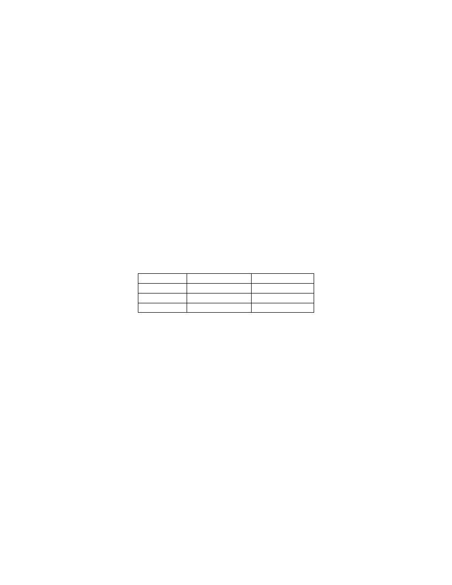
the QR factorization
Function
Flop count
errorQ
qr(, 0)
138
2.6803e-016
Givred
488
2.2204e-016
mgs
98
2.2206e-012
For comparison the number of flops used by the backslash operator was equal to 122 while the
pinv
command found a solution using 236 flops.
Another method for computing the least squares solution finds first the QR factorization of the
augmented matrix
[A b]
i.e.,
QR = [A b]
using one of the methods discussed above. The least
squares solution
x
is then found solving a linear system
Ux = Qb
, where
U
is an n-by- n principal
submatrix of
R
and
Qb
is the n+1
st
column of the matrix
R
. See e.g., [7] for more details.
Function
mylsqf
implements this method
function
x = mylsqf(A, b, f, p)
% The least squares solution x to the overdetermined
% linear system Ax = b using the QR factorization.
% The input parameter f is the string holding the
% name of a function used to obtain the QR factorization.
% Fourth input parameter p is optional and should be
% set up to 0 if the reduced form of the qr function
% is used to obtain the QR factorization.
[m, n] = size(A);
if
m <= n

19
error(
'System is not overdetermined'
)
end
if
nargin == 4
[Q, R] = qr([A b],0);
else
[Q, R] = feval(f,[A b]);
end
Qb = R(1:n,n+1);
R = R(1:n,1:n);
x = R\Qb;
A choice of a numerical algorithm for solving a particular problem is often a complex task.
Factors that should be considered include numerical stability of a method used and accuracy of
the computed solution, to mention the most important ones. It is not our intention to discuss these
issues in this tutorial. The interested reader is referred to [5] and [3].
*& $"
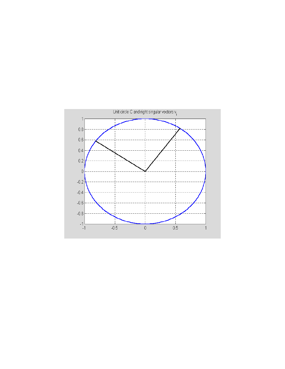
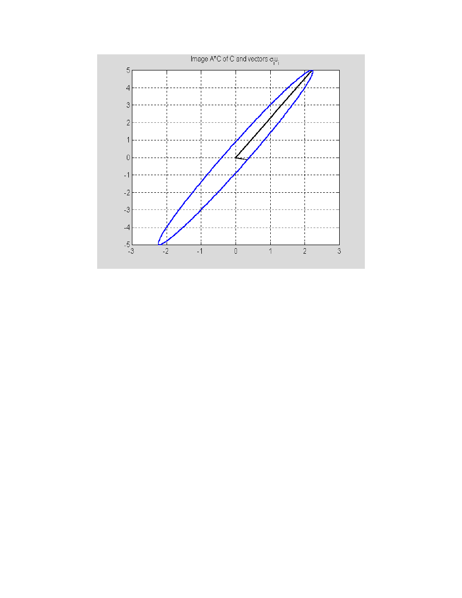
Many properties of a matrix can be derived from its singular value decomposition (SVD). The
SVD is motivated by the following fact: the image of the unit sphere under the m-by-n matrix is a
hyperellipse. Function
SVDdemo
takes a 2-by-2 matrix and generates two graphs: the original
circle together with two perpendicular vectors and their images under the transformation used. In
the example that follows the function under discussion a unit circle
C
with center at the origin is
transformed using a 2-by-2 matrix
A
.
function
SVDdemo(A)
% This illustrates a geometric effect of the application
% of the 2-by-2 matrix A to the unit circle C.
t = linspace(0,2*pi,200);
x = sin(t);
y = cos(t);
[U,S,V] = svd(A);
vx = [0 V(1,1) 0 V(1,2)];
vy = [0 V(2,1) 0 V(2,2)];
axis equal
h1_line = plot(x,y,vx,vy);
set(h1_line(1),
'LineWidth'
,1.25)
set(h1_line(2),
'LineWidth'
,1.25,
'Color'
,[0 0 0])
grid
title(
'Unit circle C and right singular vectors v_i'
)
pause(5)
w = [x;y];
z = A*w;
U = U*S;
udx = [0 U(1,1) 0 U(1,2)];
udy = [0 U(2,1) 0 U(2,2)];
figure
h1_line = plot(udx,udy,z(1,:),z(2,:));
set(h1_line(2),
'LineWidth'
,1.25,
'Color'
,[0 0 1])
set(h1_line(1),
'LineWidth'
,1.25,
'Color'
,[0 0 0])
grid
20
title(
'Image A*C of C and vectors \sigma_iu_i'
)
Define a matrix
A = [1 2;3 4];
Then
SVDdemo(A)
21
The full form of the singular value decomposition of the m-by-n matrix
A
(real or complex) is the
factorization of the form A
= USV
*
, where
U
and
V
are unitary matrices of dimensions m and n,
respectively and
S
is an m-by-n diagonal matrix with nonnegative diagonal entries stored in the
nonincreasing order. Columns of matrices
U
and
V
are called the left singular vectors and the
right singular vectors, respectively. The diagonal entries of
S
are the singular values of the
matrix
A
. MATLAB's function
svd
computes matrices of the SVD of
A
by invoking the
command
[U, S, V] = svd(A)
. The reduced form of the SVD of the matrix
A
is computed using
function
svd
with a second input parameter being set to zero
[U, S, V] = svd(A, 0)
. If
m > n
, then
only the first n columns of
U
are computed and
S
is an n-by-n matrix.
Computation of the SVD of a matrix is a nontrivial task. A common method used nowadays is the
two-phase method. Phase one reduces a given matrix
A
to an upper bidiagonal form using the
Golub-Kahan method. Phase two computes the SVD of
A
using a variant of the QR factorization.
Function
mysvd
implements a method proposed in Problem 4.15 in [4]. This code works for
the 2-by-2 real matrices only.
function
[U, S, V] = mysvd(A)
% Singular value decomposition A = U*S*V'of a
% 2-by-2 real matrix A. Matrices U and V are orthogonal.
% The left and the right singular vectors of A are stored
% in columns of matrices U and V,respectively. Singular
% values of A are stored, in the nonincreasing order, on
% the main diagonal of the diagonal matrix S.

22
if
A == zeros(2)
S = zeros(2);
U = eye(2);
V = eye(2);
return
end
[S, G] = symmat(A);
[S, J] = diagmat(S);
U = G'*J;
V = J;
d = diag(S);
s = sign(d);
for
j=1:2
if
s(j) < 0
U(:,j) = -U(:,j);
end
end
d = abs(d);
S = diag(d);
if
d(1) < d(2)
d = flipud(d);
S = diag(d);
U = fliplr(U);
V = fliplr(V);
end
In order to run this function two other functions
symmat
and
diagmat
must be in MATLAB's
search path
function
[S, G] = symmat(A)
% Symmetric 2-by-2 matrix S from the matrix A. Matrices
% A, S, and G satisfy the equation G*A = S, where G
% is the Givens plane rotation.
if
A(1,2) == A(2,1)
S = A;
G = eye(2);
return
end
t = (A(1,1) + A(2,2))/(A(1,2) - A(2,1));
s = 1/sqrt(1 + t^2);
c = -t*s;
G(1,1) = c;
G(2,2) = c;
G(1,2)= s;
G(2,1) = -s;
S = G*A;
function
[D, G] = diagmat(A);
% Diagonal matrix D obtained by an application of the
% two-sided Givens rotation to the matrix A. Second output
% parameter G is the Givens rotation used to diagonalize
% matrix A, i.e., G.'*A*G = D.

23
if
A ~= A'
error(
'Matrix must be symmetric'
)
end
if
abs(A(1,2)) < eps & abs(A(2,1)) < eps
D = A;
G = eye(2);
return
end
r = roots([-1 (A(1,1)-A(2,2))/A(1,2) 1]);
[t, k] = min(abs(r));
t = r(k);
c = 1/sqrt(1+t^2);
s = c*t;
G = zeros(size(A));
G(1,1) = c;
G(2,2) = c;
G(1,2) = s;
G(2,1) = -s;
D = G.'*A*G;
Let
A = [1 2;3 4];
Then
[U,S,V] = mysvd(A)
U =
0.4046 -0.9145
0.9145 0.4046
S =
5.4650 0
0 0.3660
V =
0.5760 0.8174
0.8174 -0.5760
To verify this result we compute
AC = U*S*V'
AC =
1.0000 2.0000
3.0000 4.0000
and the relative error in the computed SVD decomposition
norm(AC-A)/norm(A)
ans =
1.8594e-016

24
Another algorithm for computing the least squares solution
x
of the overdetermined linear system
Ax = b
utilizes the singular value decomposition of
A
. Function
lsqsvd
should be used for ill-
conditioned or rank deficient matrices.
function
x = lsqsvd(A, b)
% The least squares solution x to the overdetermined
% linear system Ax = b using the reduced singular
% value decomposition of A.
[m, n] = size(A);
if
m <= n
error(
'System must be overdetermined'
)
end
[U,S,V] = svd(A,0);
d = diag(S);
r = sum(d > 0);
b1 = U(:,1:r)'*b;
w = d(1:r).\b1;
x = V(:,1:r)*w;
re = b - A*x;
% One step of the iterative
b1 = U(:,1:r)'*re;
%
refinement
w = d(1:r).\b1;
e = V(:,1:r)*w;
x = x + e;
The linear system with
A = ones(6,3); b = ones(6,1);
is ill-conditioned and rank deficient. Therefore the least squares solution to this system is not
unique
x = lsqsvd(A,b)
x =
0.3333
0.3333
0.3333
Another application of the SVD is for computing the pseudoinverse of a matrix. Singular or
rectangular matrices always possess the pseudoinverse matrix. Let the matrix
A
be defined as
follows
A = [1 2 3;4 5 6]
A =
1 2 3
4 5 6

25
Its pseudoinverse is
B = pinv(A)
B =
-0.9444 0.4444
-0.1111 0.1111
0.7222 -0.2222
The pseudoinverse
B
of the matrix
A
satisfy the Penrose conditions
ABA = A, BAB = B, (AB)
T
= AB, (BA)
T
= BA
We will verify the first condition only
norm(A*B*A-A)
ans =
3.6621e-015
and leave it to the reader to verify the remaining ones.
+"&$
The matrix eigenvalue problem, briefly discussed in Tutorial 3, is one of the central problems in
the numerical linear algebra. It is formulated as follows.
Given a square matrix
A = [a
ij
]
,
1
i, j n
, find a nonzero vector
x
n
and a number
that
satisfy the equation
Ax =
x
. Number
is called the eigenvalue of the matrix
A
and
x
is the
associated right eigenvector of
A
.
In this section we will show how to localize the eigenvalues of a matrix using celebrated
Gershgorin's Theorem. Also, we will present MATLAB's code for computing the dominant
eigenvalue and the associated eigenvector of a matrix. The QR iteration for computing all
eigenvalues of the symmetric matrices is also discussed.
Gershgorin Theorem states that each eigenvalue
of the matrix
A
satisfies at least one of the
following inequalities
|
- a
kk
|
r
k
,
where
r
k
is the sum of all off-diagonal entries in row
k
of the
matrix
|A|
(see, e.g., [1], pp.400-403 for more details). Function
Gershg
computes the centers and
the radii of the Gershgorin circles of the matrix
A
and plots all Gershgorin circles. The
eigenvalues of the matrix
A
are also displayed.
function
[C] = Gershg(A)
% Gershgorin's circles C of the matrix A.
d = diag(A);
cx = real(d);
cy = imag(d);
B = A - diag(d);

26
[m, n] = size(A);
r = sum(abs(B'));
C = [cx cy r(:)];
t = 0:pi/100:2*pi;
c = cos(t);
s = sin(t);
[v,d] = eig(A);
d = diag(d);
u1 = real(d);
v1 = imag(d);
hold on
grid on
axis equal
xlabel(
'Re'
)
ylabel(
'Im'
)
h1_line = plot(u1,v1,
'or'
);
set(h1_line,
'LineWidth'
,1.5)
for
i=1:n
x = zeros(1,length(t));
y = zeros(1,length(t));
x = cx(i) + r(i)*c;
y = cy(i) + r(i)*s;
h2_line = plot(x,y);
set(h2_line,
'LineWidth'
,1.2)
end
hold off
title(
'Gershgorin circles and the eigenvalues of a'
)
To illustrate functionality of this function we define a matrix
A
, where
A = [1 2 3;3 4 9;1 1 1];
Then
C = Gershg(A)
C =
1 0 5
4 0 12
1 0 2
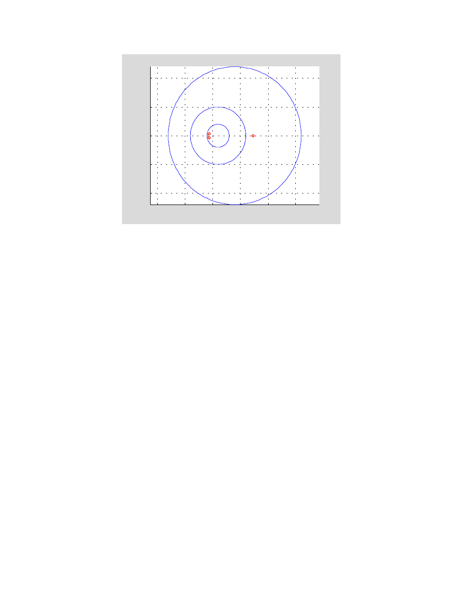
27
-10
-5
0
5
10
15
-10
-5
0
5
10
Re
Im
Gershgorin circles and the eigenvalues of a matrix
Information about each circle (coordinates of the origin and its radius) is contained in successive
rows of the matrix
C
.
It is well known that the eigenvalues are sensitive to small changes in the entries of the matrix
(see, e.g., [3]). The condition number of the simple eigenvalue
of the matrix
A
is defined as
follows
Cond(
) = 1/|y
T
x|
where
y
and
x
are the left and right eigenvectors of
A
, respectively with
||x||
2
= ||y||
2
= 1
. Recall
that a nonzero vector
y
is said to be a left eigenvector of
A
if
y
T
A =
y
T
. Clearly
Cond(
) 1
.
Function
eigsen
computes the condition number of all eigenvalues of a matrix.
function
s = eigsen(A)
% Condition numbers s of all eigenvalues of the diagonalizable
% matrix A.
[n,n] = size(A);
[v1,la1] = eig(A);
[v2,la2] = eig(A');
[d1, j] = sort(diag(la1));
v1 = v1(:,j);
[d2, j] = sort(diag(la2));
v2 = v2(:,j);
s = [];
for
i=1:n
v1(:,i) = v1(:,i)/norm(v1(:,i));
v2(:,i) = v2(:,i)/norm(v2(:,i));
s = [s;1/abs(v1(:,i)'*v2(:,i))];
end

28
In this example we will illustrate sensitivity of the eigenvalues of the celebrated Wilkinson's
matrix
W
. Its is an upper bidiagonal 20-by-20 matrix with diagonal entries 20, 19, … , 1. The
superdiagonal entries are all equal to 20. We create this matrix using some MATLAB functions
that are discussed in Section 4.9.
W = spdiags([(20:-1:1)', 20*ones(20,1)],[0 1], 20,20);
format long
s = eigsen(full(W))
s =
1.0e+012 *
0.00008448192546
0.00145503286853
0.01206523295175
0.06389158525507
0.24182386727359
0.69411856608888
1.56521713930244
2.83519277292867
4.18391920177580
5.07256664475500
5.07256664475500
4.18391920177580
2.83519277292867
1.56521713930244
0.69411856608888
0.24182386727359
0.06389158525507
0.01206523295175
0.00145503286853
0.00008448192546
Clearly all eigenvalues of the Wilkinson's matrix are sensitive.
Let us perturb the
w
20,1
entry of
W
W(20,1)=1e-5;
and next compute the eigenvalues of the perturbed matrix
eig(full(W))
ans =
-1.00978219090288
-0.39041284468158 + 2.37019976472684i
-0.39041284468158 - 2.37019976472684i
1.32106082150033 + 4.60070993953446i
1.32106082150033 - 4.60070993953446i
3.88187526711025 + 6.43013503466255i
3.88187526711025 - 6.43013503466255i
7.03697639135041 + 7.62654906220393i

29
7.03697639135041 - 7.62654906220393i
10.49999999999714 + 8.04218886506797i
10.49999999999714 - 8.04218886506797i
13.96302360864989 + 7.62654906220876i
13.96302360864989 - 7.62654906220876i
17.11812473289285 + 6.43013503466238i
17.11812473289285 - 6.43013503466238i
19.67893917849915 + 4.60070993953305i
19.67893917849915 - 4.60070993953305i
21.39041284468168 + 2.37019976472726i
21.39041284468168 - 2.37019976472726i
22.00978219090265
Note a dramatic change in the eigenvalues.
In some problems only selected eigenvalues and associated eigenvectors are needed. Let the
eigenvalues
{
k
}
be rearranged so that
|
1
| > |
2
|
… |
n
|
. The dominant eigenvalue
1
and/or
the associated eigenvector can be found using one of the following methods: power iteration,
inverse iteration, and Rayleigh quotient iteration. Functions
powerit
and
Rqi
implement the first
and the third method, respectively.
function
[la, v] = powerit(A, v)
% Power iteration with the Rayleigh quotient.
% Vector v is the initial estimate of the eigenvector of
% the matrix A. Computed eigenvalue la and the associated
% eigenvector v satisfy the inequality% norm(A*v - la*v,1) < tol,
% where tol = length(v)*norm(A,1)*eps.
if
norm(v) ~= 1
v = v/norm(v);
end
la = v'*A*v;
tol = length(v)*norm(A,1)*eps;
while
norm(A*v - la*v,1) >= tol
w = A*v;
v = w/norm(w);
la = v'*A*v;
end
function
[la, v] = Rqi(A, v, iter)
% The Rayleigh quotient iteration.
% Vector v is an approximation of the eigenvector associated with the
% dominant eigenvalue la of the matrix A. Iterative process is
% terminated either if norm(A*v - la*v,1) < norm(A,1)*length(v)*eps
% or if the number of performed iterations reaches the allowed number
% of iterations iter.
if
norm(v) > 1
v = v/norm(v);
end
la = v'*A*v;
tol = norm(A,1)*length(v)*eps;
for
k=1:iter

30
if
norm(A*v - la*v,1) < tol
return
else
w = (A - la*eye(size(A)))\v;
v = w/norm(w);
la = v'*A*v;
end
end
Let ( [7], p.208, Example 27.1)
A = [2 1 1;1 3 1;1 1 4]; v = ones(3,1);
Then
format long
flops(0)
[la, v] = powerit(A, v)
la =
5.21431974337753
v =
0.39711254978701
0.52065736843959
0.75578934068378
flops
ans =
3731
Using function
Rqi
, for computing the dominant eigenpair of the matrix
A
, we obtain
flops(0)
[la, v] = Rqi(A,ones(3,1),5)
la =
5.21431974337754
v =
0.39711254978701
0.52065736843959
0.75578934068378
flops
ans =
512

31
Once the dominant eigenvalue (eigenpair) is computed one can find another eigenvalue or
eigenpair by applying a process called deflation. For details the reader is referred to [4],
pp. 127-128.
function
[l2, v2, B] = defl(A, v1)
% Deflated matrix B from the matrix A with a known eigenvector v1 of A.
% The eigenpair (l2, v2) of the matrix A is computed.
% Functions Housv, Houspre, Housmvp and Rqi are used
% in the body of the function defl.
n = length(v1);
v1 = Housv(v1);
C = Houspre(v1,A);
B = [];
for
i=1:n
B = [B Housmvp(v1,C(i,:))];
end
l1 = B(1,1);
b = B(1,2:n);
B = B(2:n,2:n);
[l2, y] = Rqi(B, ones(n-1,1),10);
if
l1 ~= l2
a = b*y/(l2-l1);
v2 = Housmvp(v1,[a;y]);
else
v2 = v1;
end
Let
A
be an 5-by-5 Pei matrix, i.e.,
A = ones(5)+diag(ones(5,1))
A =
2 1 1 1 1
1 2 1 1 1
1 1 2 1 1
1 1 1 2 1
1 1 1 1 2
Its dominant eigenvalue is
1
= 6
and all the remaining eigenvalues are equal to one. To compute
the dominant eigenpair of
A
we use function
Rqi
[l1,v1] = Rqi(A,rand(5,1),10)
l1 =
6.00000000000000
v1 =
0.44721359549996
0.44721359549996
0.44721359549996
0.44721359549996
0.44721359549996
and next apply function
defl
to compute another eigenpair of
A

32
[l2,v2] = defl(A,v1)
l2 =
1.00000000000000
v2 =
-0.89442719099992
0.22360679774998
0.22360679774998
0.22360679774998
0.22360679774998
To check these results we compute the norms of the "residuals"
[norm(A*v1-l1*v1);norm(A*v2-l2*v2)]
ans =
1.0e-014 *
0.07691850745534
0.14571016336181
To this end we will deal with the symmetric eigenvalue problem. It is well known that the
eigenvalues of a symmetric matrix are all real. One of the most efficient algorithms is the QR
iteration with or without shifts. The algorithm included here is the two-phase algorithm. Phase
one reduces a symmetric matrix
A
to the symmetric tridiagonal matrix
T
using MATLAB's
function
hess
. Since
T
is orthogonally similar to
A
,
sp(A) = sp(T)
. Here
sp
stands for the
spectrum of a matrix. During the phase two the off diagonal entries of
T
are annihilated. This is
an iterative process, which theoretically is an infinite one. In practice, however, the off diagonal
entries approach zero fast. For details the reader is referred to [2] and [7].
Function
qrsft
computes all eigenvalues of the symmetric matrix
A
. Phase two uses Wilkinson's
shift. The latter is computed using function
wsft
.
function
[la, v] = qrsft(A)
% All eigenvalues la of the symmetric matrix A.
% Method used: the QR algorithm with Wilkinson's shift.
% Function wsft is used in the body of the function qrsft.
[n, n] = size(A);
A = hess(A);
la = [];
i = 0;
while
i < n
[j, j] = size(A);
if
j == 1
la = [la;A(1,1)];
return
end
mu = wsft(A);
[Q, R] = qr(A - mu*eye(j));
A = R*Q + mu*eye(j);

33
if
abs(A(j,j-1))< 10*(abs(A(j-1,j-1))+abs(A(j,j)))*eps
la = [la;A(j,j)];
A = A(1:j-1,1:j-1);
i = i + 1;
end
end
function
mu = wsft(A)
% Wilkinson's shift mu of the symmetric matrix A.
[n, n] = size(A);
if
A == diag(diag(A))
mu = A(n,n);
return
end
mu = A(n,n);
if
n > 1
d = (A(n-1,n-1)-mu)/2;
if
d ~= 0
sn = sign(d);
else
sn = 1;
end
bn = A(n,n-1);
mu = mu - sn*bn^2/(abs(d) + sqrt(d^2+bn^2));
end
We will test function
qrsft
on the matrix
A
used earlier in this section
A = [2 1 1;1 3 1;1 1 4];
la = qrsft(A)
la =
5.21431974337753
2.46081112718911
1.32486912943335
Function
eigv
computes both the eigenvalues and the eigenvectors of a symmetric matrix
provided the eigenvalues are distinct. A method for computing the eigenvectors is discussed in
[1], Algorithm 8.10.2, pp. 452-454
function
[la, V] = eigv(A)
% Eigenvalues la and eigenvectors V of the symmetric
% matrix A with distinct eigenvalues.
V = [];
[n, n] = size(A);
[Q,T] = schur(A);
la = diag(T);

34
if
nargout == 2
d = diff(sort(la));
for
k=1:n-1
if
d(k) < 10*eps
d(k) = 0;
end
end
if
~all(d)
disp(
'Eigenvalues must be distinct'
)
else
for
k=1:n
U = T - la(k)*eye(n);
t = U(1:k,1:k);
y1 = [];
if
k>1
t11 = t(1:k-1,1:k-1);
s = t(1:k-1,k);
y1 = -t11\s;
end
y = [y1;1];
z = zeros(n-k,1);
y = [y;z];
v = Q*y;
V = [V v/norm(v)];
end
end
end
We will use this function to compute the eigenvalues and the eigenvectors of the matrix
A
of the
last example
[la, V] = eigv(A)
la =
1.32486912943335
2.46081112718911
5.21431974337753
V =
0.88765033882045 -0.23319197840751 0.39711254978701
-0.42713228706575 -0.73923873953922 0.52065736843959
-0.17214785894088 0.63178128111780 0.75578934068378
To check these results let us compute the residuals
Av -
v
A*V-V*diag(la)
ans =
1.0e-014 *
0 -0.09992007221626 0.13322676295502
-0.02220446049250 -0.42188474935756 0.44408920985006
0 0.11102230246252 -0.13322676295502

35
,$
MATLAB has several built-in functions for computations with sparse matrices. A partial list of
these functions is included here.
Function
Description
condest
Condition estimate for sparse matrix
eigs
Few eigenvalues
find
Find indices of nonzero entries
full
Convert sparse matrix to full matrix
issparse
True for sparse matrix
nnz
Number of nonzero entries
nonzeros
Nonzero matrix entries
sparse
Create sparse matrix
spdiags
Sparse matrix formed from diagonals
speye
Sparse identity matrix
spfun
Apply function to nonzero entries
sprand
Sparse random matrix
sprandsym
Sparse random symmetric matrix
spy
Visualize sparsity pattern
svds
Few singular values
Function
spy
works for matrices in full form as well.
Computations with sparse matrices
The following MATLAB functions work with sparse matrices:
chol
,
det
,
inv
,
jordan
,
lu
,
qr
,
size
,
\
.
Command
sparse
is used to create a sparse form of a matrix.
Let
A = [0 0 1 1; 0 1 0 0; 0 0 0 1];
Then
B = sparse(A)
B =
(2,2) 1
(1,3) 1
(1,4) 1
(3,4) 1
Command
full
converts a sparse form of a matrix to the full form

36
C = full(B)
C =
0 0 1 1
0 1 0 0
0 0 0 1
Command
sparse
has the following syntax
sparse(k,l,s,m,n)
where
k
and
l
are arrays of row and column indices, respectively,
s
ia an array of nonzero
numbers whose indices are specified in
k
and
l
, and
m
and
n
are the row and column dimensions,
respectively.
Let
S = sparse([1 3 5 2], [2 1 3 4], [1 2 3 4], 5, 5)
S =
(3,1) 2
(1,2) 1
(5,3) 3
(2,4) 4
F = full(S)
F =
0 1 0 0 0
0 0 0 4 0
2 0 0 0 0
0 0 0 0 0
0 0 3 0 0
To create a sparse matrix with several diagonals parallel to the main diagonal one can use the
command
spdiags
. Its syntax is shown below
spdiags(B, d, m, n)
The resulting matrix is an m-by-n sparse matrix. Its diagonals are the columns of the matrix
B
.
Location of the diagonals are described in the vector
d
.
Function
mytrid
creates a sparse form of the tridiagonal matrix with constant entries along the
diagonals.
function
T = mytrid(a,b,c,n)
% The n-by-n tridiagonal matrix T with constant entries
% along diagonals. All entries on the subdiagonal, main
% diagonal,and the superdiagonal are equal a, b, and c,
% respectively.
37
e = ones(n,1);
T = spdiags([a*e b*e c*e],-1:1,n,n);
To create a symmetric 6-by-6-tridiagonal matrix with all diagonal entries are equal 4 and all
subdiagonal and superdiagonal entries are equal to one execute the following command
T = mytrid(1,4,1,6);
Function
spy
creates a graph of the matrix.
The nonzero entries are displayed as the dots.
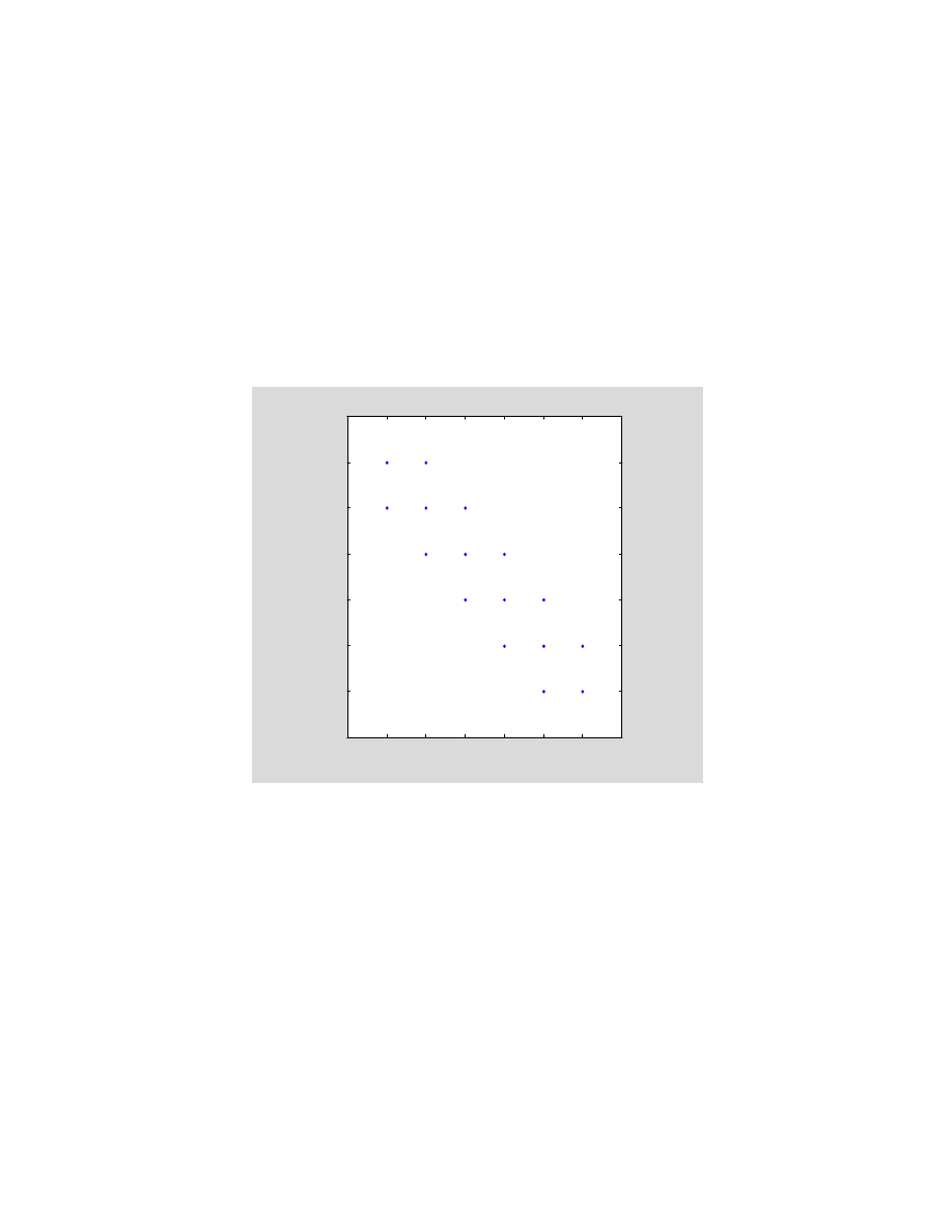
spy( T )
0
1
2
3
4
5
6
7
0
1
2
3
4
5
6
7
nz = 16
The following is the example of a sparse matrix created with the aid of the nonsparse matrix
magic
spy(rem(magic(16),2))

38
0
5
10
15
0
2
4
6
8
10
12
14
16
nz = 128
Using a sparse form rather than the full form of a matrix one can reduce a number of flops used.
Let
A = sprand(50,50,.25);
The above command generates a 50-by-50 random sparse matrix
A
with a density of about 25%.
We will use this matrix to solve a linear system
Ax = b
with
b = ones(50,1);
Number of flops used is determined in usual way
flops(0)
A\b;
flops
ans =
54757

39
Using the full form of
A
the number of flops needed to solve the same linear system is
flops(0)
full(A)\b;
flops
ans =
72014

40
-
[1] B.N. Datta, Numerical Linear Algebra and Applications, Brooks/Cole Publishing Company,
Pacific Grove, CA, 1995.
[2] J.W. Demmel, Applied Numerical Linear Algebra, SIAM, Philadelphia, PA, 1997.
[3] G.H. Golub and Ch.F. Van Loan, Matrix Computations, Second edition, Johns Hopkins
University Press, Baltimore, MD, 1989.
[4] M.T. Heath, Scientific Computing: An Introductory Survey, McGraw-Hill, Boston, MA,
1997.
[5] N.J. Higham, Accuracy and Stability of Numerical Algorithms, SIAM, Philadelphia, PA,
1996.
[6] R.D. Skeel and J.B. Keiper, Elementary Numerical Computing with Mathematica,
McGraw-Hill, New York, NY, 1993.
[7] L.N. Trefethen and D. Bau III, Numerical Linear Algebra, SIAM, Philadelphia, PA, 1997.

41
.
1.
Let
A
by an n-by-n matrix and let
v
be an n-dimensional vector. Which of the
following methods is faster?
(i)
(v*v')*A
(ii)
v*(v'*A)
2.
Suppose that
L
n x n
is lower triangular and
b
n
. Write MATLAB function
x = ltri(L, b)
that computes a solution
x
to the linear system
Lx = b
.
3. Repeat Problem 2 with
L
being replaced by the upper triangular matrix
U
. Name
your function
utri(U, b)
.
4.
Let
A
n x n
be a triangular matrix. Write a function
dettri(A)
that computes the
determinant of the matrix
A
.
5.
Write MATLAB function
MA = Gausspre(A, m, k)
that overwrites matrix
A
n x p
with
the product
MA
, where
M
n x n
is the Gauss transformation which is determined by the
Gauss vector
m
and its column index
k
.
Hint: You may wish to use the following formula
MA = A – m(e
k
T
A)
.
6.
A system of linear equations
Ax = b
, where
A
is a square matrix, can be solved applying
successively Gauss transformations to the augmented matrix
[A, b]
. A solution
x
then can be
found using back substitution, i.e., solving a linear system with an upper triangular matrix.
Using functions
Gausspre
of Problem 5,
Gaussv
described in Section 4.3, and
utri
of
Problem 3, write a function
x =
sol(A, b)
which computes a solution
x
to the linear system
Ax = b
.
7.
Add a few lines of code to the function
sol
of Problem 6 to compute the determinant of the
matrix
A
. The header of your function might look like this function
[x, d] = sol(A, b)
. The
second output parameter
d
stands for the determinant of
A
.
8.
The purpose of this problem is to test function
sol
of Problem 6.
(i)
Construct at least one matrix
A
for which function
sol
fails to compute a solution.
Explain why it happened.
(ii)
Construct at least one matrix
A
for which the computed solution
x
is poor. For
comparison of a solution you found using function
sol
with an acceptable solution
you may wish to use MATLAB's backslash operator
\
. Compute the relative error in
x
. Compare numbers of flops used by function
sol
and MATLAB's command
\
.
Which of these methods is faster in general?
9.
Given a square matrix
A
. Write MATLAB function
[L, U] = mylu(A)
that computes the LU
decomposition of
A
using partial pivoting.

42
10.
Change your working format to
format long e
and run function
mylu
of Problem 11on the
following matrices
(i)
A = [eps 1; 1 1]
(ii)
A = [1 1; eps 1]
(iii)
A = hilb(10)
(iv)
A = rand(10)
In each case compute the error
A - LU
F
.
11.
Let
A
be a tridiagonal matrix that is either diagonally dominant or positive definite.
Write MATLAB's function
[L, U] =
trilu(a, b, c)
that computes the LU factorization
of
A
. Here
a
,
b
, and
c
stand for the subdiagonal, main diagonal, and superdiagonal
of
A
, respectively.
12.
The following function computes the Cholesky factor
L
of the symmetric positive
definite matrix
A
. Matrix
L
is lower triangular and satisfies the equation
A = LL
T
.
function
L = mychol(A)
% Cholesky factor L of the matrix A; A = L*L'.
[n, n] = size(A);
for
j=1:n
for
k=1:j-1
A(j:n,j) = A(j:n,j) - A(j:n,k)*A(j,k);
end
A(j,j) = sqrt(A(j,j));
A(j+1:n,j) = A(j+1:n,j)/A(j,j);
end
L = tril(A);
Add a few lines of code that generates the error messages when
A
is neither
•
symmetric nor
•
positive definite
Test the modified function
mychol
on the following matrices
(i)
A = [1 2 3; 2 1 4; 3 4 1]
(ii)
A = rand(5)
13.
Prove that any 2-by-2 Householder reflector is of the form
H = [cos
sin ; sin -cos ]
. What is the Householder reflection vector
u
of
H
?
14.
Find the eigenvalues and the associated eigenvectors of the matrix
H
of Problem 13.
15.
Write MATLAB function
[Q, R] = myqr(A)
that computes a full QR factorization
A = QR
of
A
m x n
with
m
n
using Householder reflectors. The output matrix
Q
is an m-
by-m orthogonal matrix and
R
is an m-by-n upper triangular with zero entries in rows n+1
through m.

43
Hint: You may wish to use function
Housprod
in the body of the function
myqr
.
16.
Let
A
be an n-by-3 random matrix generated by the MATLAB function
rand
. In this
exercise you are to plot the error
A - QR
F
versus n for n = 3, 5, … , 25. To
compute the QR factorization of
A
use the function
myqr
of Problem 15. Plot the graph of the
computed errors using MATLAB's function
semilogy
instead of the function
plot
. Repeat this
experiment several times. Does the error increase as n does?
17.
Write MATLAB function
V = Vandm(t, n)
that generates Vandermonde's matrix
V
used in the polynomial least-squares fit. The degree of the approximating polynomial
is
n
while the x-coordinates of the points to be fitted are stored in the vector
t
.
18.
In this exercise you are to compute coefficients of the least squares polynomials using four
methods, namely the normal equations, the QR factorization, modified Gram-Schmidt
orthogonalization and the singular value decomposition.
Write MATLAB function
C = lspol(t, y, n)
that computes coefficients of the
approximating polynomials. They should be saved in columns of the matrix
C
(n+1) x 4
. Here
n
stands for the degree of the polynomial,
t
and
y
are the vectors
holding the x- and the y-coordinates of the points to be approximated, respectively.
Test your function using
t = linspace(1.4, 1.8)
,
y = sin(tan(t)) – tan(sin(t))
,
n = 2, 4, 8
.
Use
format long
to display the output to the screen.
Hint: To create the Vandermonde matrix needed in the body of the function
lspol
you
may wish to use function
Vandm
of Problem 17.
19.
Modify function
lspol
of Problem 18 adding a second output parameter
err
so that
the header of the modified function should look like this
function
[C, err] = lspol(t, y, n)
. Parameter
err
is the least squares error in the computed
solution
c
to the overdetermined linear system
Vc
y
. Run the modified function on the data
of Problem 18. Which of the methods used seems to produce the least reliable numerical
results? Justify your answer.
20.
Write MATLAB function
[r, c] = nrceig(A)
that computes the number of real and
complex eigenvalues of the real matrix
A
. You cannot use MATLAB function
eig
. Run
function
nrceig
on several random matrices generated by the functions
rand
and
randn
.
Hint: You may wish to use the following MATLAB functions
schur
,
diag
,
find
. Note that
the
diag
function takes a second optional argument.
21.
Assume that an eigenvalue of a matrix is sensitive if its condition number is
greater than 10
3
. Construct an n-by-n matrix (
5
n 10
) whose all eigenvalues are
real and sensitive.
22.
Write MATLAB function
A = pent(a, b, c, d, e, n)
that creates the full form of the
n-by-n pentadiagonal matrix
A
with constant entries
a
along the second subdiagonal, constant
entries
b
along the subdiagonal, etc.
23.
Let
A = pent(1, 26, 66, 26, 1, n)
be an n-by-n symmetric pentadiagonal matrix
generated by function
pent
of Problem 22. Find the eigenvalue decomposition
A = Q
Q
T
of
A
for various values of
n
. Repeat this experiment using random numbers in the
band of the matrix
A
. Based on your observations, what conjecture can be formulated about
the eigenvectors of
A
?
24.
Write MATLAB function
[la, x] = smeig(A, v)
that computes the smallest

44
(in magnitude) eigenvalue of the nonsingular matrix
A
and the associated
eigenvector
x
. The input parameter
v
is an estimate of the eigenvector of
A
that is
associated with the largest (in magnitude) eigenvalue of
A
.
25.
In this exercise you are to experiment with the eigenvalues and eigenvectors of the
partitioned matrices. Begin with a square matrix
A
with known eigenvalues and
eigenvectors. Next construct a matrix
B
using MATLAB's built-in function
repmat
to define the matrix
B
as
B = repmat(A, 2, 2)
. Solve the matrix eigenvalue
problem for the matrix
B
and compare the eigenvalues and eigenvectors of matrices
A
and
B
. You may wish to continue in this manner using larger values for the second
and third parameters in the function
repmat
. Based on the results of your experiment,
what conjecture about the eigenvalues and eigenvectors of
B
can be formulated?
Wyszukiwarka
Podobne podstrony:
Numerical linear algebra in data mining
tutorial3 Using MATLAB in Linear Algebra
Linear Algebra, Infinite Dimensions, and Maple, Preface
(ebook pdf) Mathematics Abstract And Linear Algebra PJFCT5UIYCCSHOYDU7JHPAKULMLYEBKKOCB7OWA
Connell Elements of abstract and linear algebra(146s)
Elements of Abstract and Linear Algebra E H Connell
Prentice Hall Carlson & Johnson Multivariable Mathematics with Maple Linear Algebra, Vector Calcul
Soroka Linear Odd Poisson Bracket on Grassmann Algebra (2000) [sharethefiles com]
tutorial6 Linear Programming with MATLAB
więcej podobnych podstron