
Mirrors and Reflections:
The Geometry of Finite Reflection Groups
Incomplete Draft Version 01
Alexandre V. Borovik
alexandre.borovik@umist.ac.uk
Anna S. Borovik
anna.borovik@freenet.co.uk
25 February 2000

A. & A. Borovik • Mirrors and Reflections • Version 01 • 25.02.00
i
Introduction
This expository text contains an elementary treatment of finite groups gen-
erated by reflections. There are many splendid books on this subject, par-
ticularly [H] provides an excellent introduction into the theory. The only
reason why we decided to write another text is that some of the applications
of the theory of reflection groups and Coxeter groups are almost entirely
based on very elementary geometric considerations in Coxeter complexes.
The underlying ideas of these proofs can be presented by simple drawings
much better than by a dry verbal exposition. Probably for the reason of
their extreme simplicity these elementary arguments are mentioned in most
books only briefly and tangently.
We wish to emphasize the intuitive elementary geometric aspects of
the theory of reflection groups. We hope that our approach allows an
easy access of a novice mathematician to the theory of reflection groups.
This aspect of the book makes it close to [GB]. We realise, however,
that, since classical Geometry has almost completely disappeared from
the schools’ and Universities’ curricula, we need to smugle it back and
provide the student reader with a modicum of Euclidean geometry and
theory of convex polyhedra. We do not wish to appeal to the reader’s
geometric intuition without trying first to help him or her to develope
it. In particular, we decided to saturate the book with visual material.
Our sketches and diagrams are very unsophisticated; one reason for this
is that we lack skills and time to make the pictures more intricate and
aesthetically pleasing, another is that the book was tested in a M. Sc.
lecture course at UMIST in Spring 1997, and most pictures, in their even
less sophisticated versions, were first drawn on the blackboard. There was
no point in drawing pictures which could not be reproduced by students
and reused in their homework. Pictures are not for decoration, they are
indispensable (though maybe greasy and soiled) tools of the trade.
The reader will easily notice that we prefer to work with the mirrors
of reflections rather than roots. This approach is well known and fully
exploited in Chapter 5, §3 of Bourbaki’s classical text [Bou]. We have
combined it with Tits’ theory of chamber complexes [T] and thus made
the exposition of the theory entirely geometrical.
The book contains a lot of exercises of different level of difficulty. Some
of them may look irrelevant to the subject of the book and are included for
the sole purpose of developing the geometric intuition of a student. The
more experienced reader may skip most or all exercises.

ii
Prerequisites
Formal prerequisites for reading this book are very modest. We assume
the reader’s solid knowledge of Linear Algebra, especially the theory of
orthogonal transformations in real Euclidean spaces. We also assume that
they are familiar with the following basic notions of Group Theory:
groups; the order of a finite group; subgroups; normal sub-
groups and factorgroups; homomorphisms and isomorphisms;
permutations, standard notations for them and rules of their
multiplication; cyclic groups; action of a group on a set.
You can find this material in any introductory text on the subject. We
highly recommend a splendid book by M. A. Armstrong [A] for the first
reading.

A. & A. Borovik • Mirrors and Reflections • Version 01 • 25.02.00
iii
Acknowledgements
The early versions of the text were carefully read by Robert Sandling and
Richard Booth who suggested many corrections and improvements.
Our special thanks are due to the students in the lecture course at
UMIST in 1997 where the first author tested this book:
Bo Ahn, Ay¸se Berkman, Richard Booth, Nazia Kalsoom, Vaddna
Nuth.

iv

Contents
1
Hyperplane arrangements
1
1.1
Affine Euclidean space
AR
n
. . . . . . . . . . . . . . . . .
1
1.1.1
How to read this section . . . . . . . . . . . . . . .
1
1.1.2
Euclidean space
R
n
. . . . . . . . . . . . . . . . . .
2
1.1.3
Affine Euclidean space
AR
n
. . . . . . . . . . . . .
2
1.1.4
Affine subspaces . . . . . . . . . . . . . . . . . . . .
3
1.1.5
Half spaces
. . . . . . . . . . . . . . . . . . . . . .
5
1.1.6
Bases and coordinates . . . . . . . . . . . . . . . .
6
1.1.7
Convex sets . . . . . . . . . . . . . . . . . . . . . .
7
1.2
Hyperplane arrangements
. . . . . . . . . . . . . . . . . .
8
1.2.1
Chambers of a hyperplane arrangement . . . . . . .
8
1.2.2
Galleries . . . . . . . . . . . . . . . . . . . . . . . .
10
1.3
Polyhedra . . . . . . . . . . . . . . . . . . . . . . . . . . .
12
1.4
Isometries of
AR
n
. . . . . . . . . . . . . . . . . . . . . . .
14
1.4.1
Fixed points of groups of isometries . . . . . . . . .
14
1.4.2
Structure of Isom
AR
n
. . . . . . . . . . . . . . . .
15
1.5
Simplicial cones . . . . . . . . . . . . . . . . . . . . . . . .
20
1.5.1
Convex sets . . . . . . . . . . . . . . . . . . . . . .
20
1.5.2
Finitely generated cones . . . . . . . . . . . . . . .
20
1.5.3
Simple systems of generators . . . . . . . . . . . . .
22
1.5.4
Duality
. . . . . . . . . . . . . . . . . . . . . . . .
25
1.5.5
Duality for simplicial cones . . . . . . . . . . . . . .
25
1.5.6
Faces of a simplicial cone . . . . . . . . . . . . . . .
27
2
Mirrors, Reflections, Roots
31
2.1
Mirrors and reflections . . . . . . . . . . . . . . . . . . . .
31
2.2
Systems of mirrors . . . . . . . . . . . . . . . . . . . . . .
34
2.3
Dihedral groups . . . . . . . . . . . . . . . . . . . . . . . .
39
2.4
Root systems . . . . . . . . . . . . . . . . . . . . . . . . .
44
2.5
Planar root systems . . . . . . . . . . . . . . . . . . . . . .
46
2.6
Positive and simple systems . . . . . . . . . . . . . . . . .
49
2.7
Root system A
n−1
. . . . . . . . . . . . . . . . . . . . . . .
51
v

vi
2.8
Root systems of type C
n
and B
n
. . . . . . . . . . . . . . .
56
2.9
The root system D
n
. . . . . . . . . . . . . . . . . . . . .
60
3
Coxeter Complex
63
3.1
Chambers . . . . . . . . . . . . . . . . . . . . . . . . . . .
63
3.2
Generation by simple reflections . . . . . . . . . . . . . . .
65
3.3
Foldings . . . . . . . . . . . . . . . . . . . . . . . . . . . .
66
3.4
Galleries and paths . . . . . . . . . . . . . . . . . . . . . .
67
3.5
Action of W on C . . . . . . . . . . . . . . . . . . . . . . .
69
3.6
Labelling of the Coxeter complex . . . . . . . . . . . . . .
73
3.7
Isotropy groups . . . . . . . . . . . . . . . . . . . . . . . .
74
3.8
Parabolic subgroups
. . . . . . . . . . . . . . . . . . . . .
77
3.9
Residues . . . . . . . . . . . . . . . . . . . . . . . . . . . .
78
3.10 Generalised permutahedra . . . . . . . . . . . . . . . . . .
79
4
Classification
83
4.1
Generators and relations . . . . . . . . . . . . . . . . . . .
83
4.2
Decomposable reflection groups . . . . . . . . . . . . . . .
83
4.3
Classification of finite reflection groups . . . . . . . . . . .
85
4.4
Construction of root systems . . . . . . . . . . . . . . . . .
85
4.5
Orders of reflection groups . . . . . . . . . . . . . . . . . .
91

List of Figures
1.1
Convex and non-convex sets. . . . . . . . . . . . . . . . . .
7
1.2
Line arrangement in
AR
2
. . . . . . . . . . . . . . . . . . .
8
1.3
Polyhedra and polytopes . . . . . . . . . . . . . . . . . . .
12
1.4
A polyhedron is the union of its faces . . . . . . . . . . . .
12
1.5
The regular 2-simplex . . . . . . . . . . . . . . . . . . . . .
13
1.6
For the proof of Theorem 1.4.1 . . . . . . . . . . . . . . . .
14
1.7
Convex and non-convex sets. . . . . . . . . . . . . . . . . .
20
1.8
Pointed and non-pointed cones . . . . . . . . . . . . . . . .
22
1.9
Extreme and non-extreme vectors. . . . . . . . . . . . . . .
22
1.10 The cone generated by two simple vectors
. . . . . . . . .
24
1.11 Dual simplicial cones. . . . . . . . . . . . . . . . . . . . . .
26
2.1
Isometries and mirrors (Lemma 2.1.3). . . . . . . . . . . .
32
2.2
A closed system of mirrors. . . . . . . . . . . . . . . . . . .
35
2.3
Infinite planar mirror systems . . . . . . . . . . . . . . . .
36
2.4
Billiard . . . . . . . . . . . . . . . . . . . . . . . . . . . . .
38
2.5
For Exercise 2.2.3.
. . . . . . . . . . . . . . . . . . . . . .
39
2.6
Angular reflector . . . . . . . . . . . . . . . . . . . . . . .
40
2.7
The symmetries of the regular n-gon . . . . . . . . . . . .
42
2.8
Lengths of roots in a root system. . . . . . . . . . . . . . .
45
2.9
A planar root system (Lemma 2.5.1). . . . . . . . . . . . .
47
2.10 A planar mirror system (for the proof of Lemma 2.5.1). . .
47
2.11 The root system G
2
. . . . . . . . . . . . . . . . . . . . . .
48
2.12 The system generated by two simple roots . . . . . . . . .
50
2.13 Simple systems are obtuse (Lemma 2.6.1). . . . . . . . . .
51
2.14 Sym
n
is the group of symmetries of the regular simplex. . .
53
2.15 Root system of type A
2
. . . . . . . . . . . . . . . . . . . .
53
2.16 Hyperoctahedron and cube. . . . . . . . . . . . . . . . . .
57
2.17 Root systems B
2
and C
2
. . . . . . . . . . . . . . . . . . . .
58
2.18 Root system D
3
. . . . . . . . . . . . . . . . . . . . . . . .
61
3.1
The fundamental chamber. . . . . . . . . . . . . . . . . . .
64
3.2
The Coxeter complex BC
3
. . . . . . . . . . . . . . . . . . .
64
vii

viii
3.3
Chambers and the baricentric subdivision. . . . . . . . . .
65
3.4
Generation by simple reflections (Theorem 3.2.1). . . . . .
65
3.5
Folding . . . . . . . . . . . . . . . . . . . . . . . . . . . . .
67
3.6
Folding a path (Lemma 3.5.4) . . . . . . . . . . . . . . . .
71
3.7
Labelling of panels in the Coxeter complex BC
3
.
. . . . . . .
73
3.8
Permutahedron for Sym
4
. . . . . . . . . . . . . . . . . . .
79
3.9
Edges and mirrors (Theorem 3.10.1). . . . . . . . . . . . .
80
3.10 A convex polytope and polyhedral cone (Theorem 3.10.1).
81
3.11 A permutahedron for BC
3
. . . . . . . . . . . . . . . . . . .
82
4.1
For the proof of Theorem 4.1.1.
. . . . . . . . . . . . . . . .
84

Chapter 1
Hyperplane arrangements
1.1
Affine Euclidean space
AR
n
1.1.1
How to read this section
This section provides only a very sketchy description of the affine geometry
and can be skipped if the reader is familiar with this standard chapter of
Linear Algebra; otherwise it would make a good exercise to restore the
proofs which are only indicated in our text
1
. Notice that the section con-
tains nothing new in comparision with most standard courses of Analytic
Geometry. We simply transfer to n dimensions familiar concepts of three
dimensional geometry.
The reader who wishes to understand the rest of the course can rely on
his or her three dimensional geometric intuition. The theory of reflection
groups and associated geometric objects, root systems, has the most for-
tunate property that almost all computations and considerations can be
reduced to two and three dimensional configurations. We shall make every
effort to emphasise this intuitive geometric aspect of the theory. But, as a
warning to students, we wish to remind you that our intuition would work
only when supported by our ability to prove rigorously ‘intuitively evident’
facts.
1
To attention of students: the material of this section will not be included in the
examination.
1

2
1.1.2
Euclidean space
R
n
Let
R
n
be the Euclidean n-dimensional real vector space with canonical
scalar product ( , ). We identify
R
n
with the set of all column vectors
α =
a
1
..
.
a
n
of length n over
R, with componentwise addition and multiplication by
scalars, and the scalar product
(α, β) = α
t
β = (a
1
, . . . , a
n
)
b
1
..
.
a
n
= a
1
b
1
+ · · · + a
n
b
n
;
here
t
denotes taking the transposed matrix.
This means that we fix the canonical orthonormal basis
1
, . . . ,
n
in
R
n
, where
i
=
0
..
.
1
..
.
0
( the entry 1 is in the ith row) .
The length |α| of a vector α is defined as |α| =
p
(a, a). The angle A
between two vectors α and β is defined by the formula
cos A =
(α, β)
|α||β|
,
0
6 A < π.
If α ∈ R
n
, then
α
⊥
= { β ∈ R
n
| (α, β) = 0 }
in the linear subspace normal to α. If α 6= 0 then dim α
⊥
= n − 1.
1.1.3
Affine Euclidean space
AR
n
The real affine Euclidean space
AR
n
is simply the set of all n-tuples
a
1
, . . . , a
n
of real numbers; we call them points. If a = (a
1
, . . . , a
n
) and

A. & A. Borovik • Mirrors and Reflections • Version 01 • 25.02.00
3
b = (b
1
, . . . , b
n
) are two points, the distance r(a, b) between them is defined
by the formula
r(a, b) =
p
(a
1
− b
1
)
2
+ · · · + (a
n
− b
n
)
2
.
On of the most basic and standard facts in Mathematics states that this
distance satisfies the usual axioms for a metric: for all a, b, c ∈ R
n
,
• r(a, b) > 0;
• r(a, b) = 0 if and only if a = b;
• r(a, b) + r(b, c) > r(a, c) (the Triangle Inequality).
With any two points a and b we can associate a vector
2
in
R
n
~
ab =
b
1
− a
1
..
.
b
n
− a
n
.
If a is a point and α a vector, a + α denotes the unique point b such that
~
ab = α. The point a will be called the initial, b the terminal point of the
vector ~
ab. Notice that
r(a, b) = | ~
ab|.
The real Euclidean space
R
n
models what physicists call the system
of free vectors, i.e. physical quantities characterised by their magnitude
and direction, but whose application point is of no consequence. The n-
dimensional affine Euclidean space
AR
n
is a mathematical model of the
system of bound vectors, that is, vectors having fixed points of application.
1.1.4
Affine subspaces
Subspaces.
If U is a vector subspace in
R
n
and a is a point in
AR
n
then
the set
a + U = { a + β | β ∈ U }
is called an affine subspace in
AR
n
. The dimension dim A of the affine sub-
space A = a + U is the dimension of the vector space U . The codimension
of an affine subspace A is n − dim A.
2
It looks a bit awkward that we arrange the coordinates of points in rows, and the
coordinates of vectors in columns. The row notation is more convenient typographically,
but, since we use left notation for group actions, we have to use column vectors: if A is
a square matrix and α a vector, the notation Aα for the product of A and α requires α
to be a column vector.

4
If A is an affine subspace and a ∈ A a point then the set of vectors
~
A = { ~
ab | b ∈ A }
is a vector subspace in
R
n
; it coincides with the set
{ ~
bc | b, c ∈ A }
and thus does not depend on choice of the point a ∈ A. We shall call ~
A
the vector space of A. Notice that A = a + ~
A for any point a ∈ A. Two
affine subspaces A and B of the same dimension are parallel if ~
A = ~
B.
Systems of linear equations.
The standard theory of systems of si-
multaneous linear equaitions characterises affine subspaces as solution sets
of systems of linear equations
a
11
x
1
+ · · · + a
1n
x
n
= c
1
a
21
x
1
+ · · · + a
2n
x
n
= c
2
..
.
..
.
a
m1
x
1
+ · · · + a
mn
x
n
= c
m
.
In particular, the intersection of affine subspaces is either an affine subspace
or the empty set. The codimension of the subspace given by the system of
linear equations is the maximal number of linearly independent equations
in the system.
Points.
Points in
AR
n
are 0-dimensional affine subspaces.
Lines.
Affine subspaces of dimension 1 are called straight lines or lines.
They have the form
a +
Rα = { a + tα | t ∈ R },
where a is a point and α a non-zero vector. For any two distinct points
a, b ∈ AR
n
there is a unique line passing through them, that is, a +
R ~
ab.
The segment [a, b] is the set
[a, b] = { a + t ~
ab | 0 6 t 6 1 },
the interval (a, b) is the set
(a, b) = { a + t ~
ab | 0 < t < 1 }.

A. & A. Borovik • Mirrors and Reflections • Version 01 • 25.02.00
5
Planes.
Two dimensional affine subspaces are called planes.
If three
points a, b, c are not collinear , i.e. do not belong to a line, then there is a
unique plane containing them, namely, the plane
a +
R ~
ab +
R ~
ac = { a + u ~
ab + v ~
ac | u, v, ∈ R }.
A plane contains, for any its two distinct points, the entire line connecting
them.
Hyperplanes,
that is, affine subspaces of codimension 1, are given by
equations
a
1
x
1
+ · · · + a
n
x
n
= c.
(1.1)
If we represent the hyperplane in the vector form b + U , where U is a
(n − 1)-dimensional vector subspace of R
n
, then U = α
⊥
, where
α =
a
1
..
.
a
n
.
Two hyperplanes are either parallel or intersect along an affine subspace
of dimension n − 2.
1.1.5
Half spaces
If H is a hyperplane given by Equation 1.1 and we denote by f (x) the
linear function
f (x) = a
1
x
1
+ · · · + a
n
x
n
− c,
where x = (x
1
, . . . , x
n
), then the hyperplane divides the affine space
AR
n
in two open half spaces V
+
and V
−
defined by the inequalities f (x) > 0
and f (x) < 0. The sets V
+
and V
−
defined by the inequalities f (x)
> 0
and f (x)
6 0 are called closed half spaces. The half spaces are convex in
the following sense: if two points a and b belong to one half space, say, V
+
then the restriction of f onto the segment
[a, b] = { a + t ~
ab | 0 6 t 6 1 }
is a linear function of t which cannot take the value 0 on the segment
0
6 t 6 1. Hence, with any its two points a and b, a half space contains
the segment [a, b]. Subsets in
AR
n
with this property are called convex.
More generally, a curve is an image of the segment [0, 1] of the real line
R under a continuous map from [0, 1] to AR
n
. In particular, a segment
[a, b] is a curve, the map being t 7→ a + t ~
ab.

6
Two points a and b of a subset X ⊆ AR
n
are connected in X if there is
a curve in X containing both a and b. This is an equivalence relation, and
its classes are called connected components of X. A subset X is connected
if it consists of just one connected component, that is, any two points in
X can be connected by a curve belonging to X. Notice that any convex
set is connected; in particular, half spaces are connected.
If H is a hyperplane in
AR
n
then its two open halfspaces V
−
and V
+
are connected components of
AR
n
r H. Indeed, the halfspaces V
+
and V
−
are connected. But if we take two points a ∈ V
+
and b ∈ V
−
and consider
a curve
{ x(t) | t ∈ [0, 1] } ⊂ AR
n
connecting a = x(0) and b = x(1), then the continuous function f (x(t))
takes the values of opposite sign at the ends of the segment [0, 1] and thus
should take the value 0 at some point t
0
, 0 < t
0
< 1. But then the point
x(t
0
) of the curve belongs to the hyperplane H.
1.1.6
Bases and coordinates
Let A be an affine subspace in
AR
n
and dim A = k. If o ∈ A is an arbitrary
point and α
1
, . . . , α
k
is an orthonormal basis in ~
A then we can assign to
any point a ∈ A the coordinates (a
1
, . . . , a
k
) defined by the rule
a
i
= ( ~
oa, α
i
), i = 1, . . . , k.
This turns A into an affine Euclidean space of dimension k which can be
identified with
AR
k
. Therefore everything that we said about
AR
n
can be
applied to any affine subspace of
AR
n
.
We shall use change of coordinates in the proof of the following simple
fact.
Proposition 1.1.1 Let a and b be two distinct points in
AR
n
. The set of
all points x equidistant from a and b, i.e. such that r(a, x) = r(b, x) is a
hyperplane normal to the segment [a, b] and passing through its midpoint.
Proof.
Take the midpoint o of the segment [a, b] for the origin of an
orthonormal coordinate system in
AR
n
, then the points a and b are rep-
resented by the vectors ~
oa = α and ~
ob = −α. If x is a point with
r(a, x) = r(b, x) then we have, for the vector χ = ~
ox,
|χ − α| = |χ + α|,
(χ − α, χ − α) = (χ + α, χ + α),
(χ, χ) − 2(χ, α) + (α, α) = (χ, χ) + 2(χ, α) + (α, α),
A. & A. Borovik • Mirrors and Reflections • Version 01 • 25.02.00
7
which gives us
(χ, α) = 0.
But this is the equation of the hyperplane normal to the vector α directed
along the segment [a, b]. Obviously the hyperplane contains the midpoint
o of the segment.
1.1.7
Convex sets
Recall that a subset X ⊆ AR
n
is convex if it contains, with any points
x, y ∈ X, the segment [x, y] (Figure 1.7).
H
H
H
H
H
H
H
H
H
H
r
r
@
@
@
@
x
y
convex set
@
@
@
@
@
r
r
x
y
non-convex set
Figure 1.1: Convex and non-convex sets.
Obviously the intersection of a collection of convex sets is convex. Every
convex set is connected. Affine subspaces (in particular, hyperplanes) and
half spaces in
AR
n
are convex. If a set X is convex then so are its closure
X and interior X
◦
. If Y ⊆ AR
n
is a subset, it convex hull is defined as
the intersection of all convex sets containing it; it is the smallest convex
set containing Y .
Exercises
1.1.1 Prove that the complement to a 1-dimensional linear subspace in the
2-dimensional complex vector space
C
2
is connected.
1.1.2 In a well known textbook on Geometry [Ber] the affine Euclidean spaces
are defined as triples (A, ~
A, Φ), where ~
A is an Euclidean vector space, A a set
and Φ a faithful simply transitive action of the additive group of ~
A on A [Ber,
vol. 1, pp. 55 and 241]. Try to understand why this is the same object as the
one we discussed in this section.

8
1.2
Hyperplane arrangements
This section follows the classical treatment of the subject by Bourbaki
[Bou], with slight changes in terminology. All the results mentioned in
this section are intuitively self-evident, at least after drawing a few simple
pictures. We omit some of the proofs which can be found in [Bou, Chap. V,
§1].
1.2.1
Chambers of a hyperplane arrangement
A finite set Σ of hyperplanes in
AR
n
is called a hyperplane arrangement.
We shall call hyperplanes in Σ walls of Σ.
Given an arrangement Σ, the hyperlanes in Σ cut the space
AR
n
and
each other in pieces called faces, see the explicit definition below. We wish
to develop a terminology for the description of relative position of faces
with respect to each other.
If H is a hyperplane in
AR
n
, we say that two points a and b of
AR
n
are on the same side of H if both of them belong to one and the same of
two halfspaces V
+
, V
−
determined by H; a and b are similarly positioned
with respect to H if both of them belong simultaneously to either V
+
, H
or V
−
.
J
J
J
J
J
J
J
J
J
J
J
JJ
J
J
JJ
∞
−∞
∞
−∞
∞
−∞
q
q
q
A
a
B
b
C
c
D
E
F
G
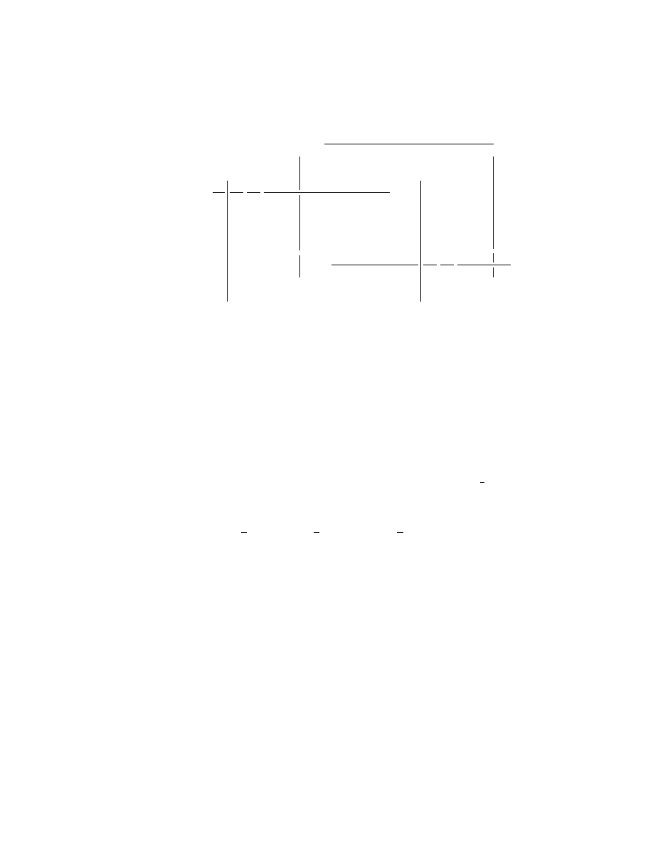
Figure 1.2:
Three lines in general position (i.e. no two lines are parallel and
three lines do not intersect in one point) divide the plane into seven open faces
A, . . . , G (chambers), nine 1-dimensional faces (edges) (−∞, a), (a, b), . . . , (c, ∞),
and three 0-dimensional faces (vertices) a, b, c. Notice that 1-dimensional faces
are open intervals.

A. & A. Borovik • Mirrors and Reflections • Version 01 • 25.02.00
9
Let Σ be a finite set of hyperplanes in
AR
n
. If a and b are points in
AR
n
, we shall say that a and b are similarly positioned with respect to Σ
and write a ∼ b if a and b are similarly positioned with respect to every
hyperplane H ∈ Σ. Obviously ∼ is an equivalence relation. Its equivalence
classes are called faces of the hyperplane arrangement Σ (Figure 1.2). Since
Σ is finite, it has only finitely many faces. We emphasise that faces are
disjoint; distinct faces have no points in common.
It easily follows from the definition that if F is a face and a hyperplane
H ∈ Σ contains a point in F then H contains F . The intersection L of
all hyperplanes in Σ which contain F is an affine subspace, it is called the
support of F . The dimension of F is the dimension of its support L.
Topological properties of faces are described by the following result.
Proposition 1.2.1 In this notation,
• F is an open convex subset of the affine space L.
• The boundary of F is the union of some set of faces of strictly smaller
dimension.
• If F and F
0
are faces with equal closures, F = F
0
, then F = F
0
.
Chambers.
By definition, chambers are faces of Σ which are not con-
tained in any hyperplane of Σ. Also chambers can be defined, in an equiv-
alent way, as connected components of
AR
n
r
[
H∈Σ
H.
Chambers are open convex subsets of
AR
n
. A panel or facet of a chamber
C is a face of dimension n − 1 on the boundary of C. It follows from the
definition that a panel P belongs to a unique hyperplane H ∈ Σ, called a
wall of the chamber C.
Proposition 1.2.2 Let C and C
0
be two chambers. The following condi-
tions are equivalent:
• C and C
0
are separated by just one hyperplane in Σ.
• C and C
0
have a panel in common.
• C and C
0
have a unique panel in common.
Lemma 1.2.3 Let C and C
0
be distinct chambers and P their common
panel. Then

10
(a) the wall H which contains P is the only wall with a notrivial inter-
section with the set C ∪ P ∪ C
0
, and
(b) C ∪ P ∪ C
0
is a convex open set.
Proof.
The set C ∪ P ∪ C
0
is a connected component of what is left
after deleting from V all hyperplanes from Σ but H. Therefore H is the
only wall in σ which intersects C ∪ P ∪ C
0
. Moreover, C ∪ P ∪ C
0
is the
intersection of open half-spaces and hence is convex.
1.2.2
Galleries
We say that chambers C and C
0
are adjacent if they have a panel in
common. Notice that a chamber is adjacent to itself. A gallery Γ is a
sequence C
0
, C
1
, . . . , C
l
of chambers such that C
i
and C
i−1
are adjacent,
for all i = 1, . . . , l. The number l is called the length of the gallery. We say
that C
0
and C
l
are connected by the gallery Γ and that C
0
and C
l
are the
endpoints of Γ. A gallery is geodesic if it has the minimal length among
all galleries connecting its endpoints. The distance d(C, D) between the
chambers C and D is the length of a geodesic gallery connecting them.
Proposition 1.2.4 Any two chambers of Σ can be connected by a gallery.
The distance d(D, C) between the chambers C and D equals to the number
of hyperplanes in Σ which separate C from D.
Proof.
Assume that C and D are separated by m hyperplanes in Σ.
Select two points c ∈ C and d ∈ D so that the segment [c, d] does not
intersect any (n − 2)-dimensional face of Σ. Then the chambers which are
intersected by the segment [c, d, ] form a gallery connecting C and D, and
it is easy to see that its length is m. To prove that m = d(C, D), consider
an arbitrary gallery C
0
, . . . , C
l
connecting C = C
0
and D = C
l
. We may
assume without loss of generality that consequent chambers C
i−1
and C
i
are distinct for all i = 1, . . . , l. For each i = 0, 1, . . . , l, chose a point
c
i
∈ C
i
. The union
[c
0
, c
1
] ∪ [c
1
, c
2
] ∪ · · · ∪ [c
l−1
, c
l
]
is connected, and by the connectedness argument each wall H which sepa-
rates C and D has to intersect one of the segments [c
i−1
, c
i
]. Let P be the
common panel of C
i−1
and C
i
. By virtue of Lemma 1.2.3(a), [c
i−1
, c
i
] ⊂
C
i−1
∪ P ∪ C
i
and H has a nontrivial intersection with C
i−1
∪ P ∪ C
i
. But
then, in view of Lemma 1.2.3(b), H contains the panel P . Therefore each

A. & A. Borovik • Mirrors and Reflections • Version 01 • 25.02.00
11
of m walls separating C from D contains the common panel of a different
pair (C
i−1
, C
i
) of adjacent chambers. It is obvious now that l
> m.
As a byproduct of this proof, we have another useful result.
Lemma 1.2.5 Assume that the endpoints ot the gallery C
0
, C
1
, . . . , C
l
lie
on the opposite sides of the wall H. Then, for some i = 1, . . . , l, the wall
H contains the common panel of consequtive chambers C
i−1
and C
i
.
We shall say in this situation that the wall H interesects the gallery
C
0
, . . . , C
l
.
Another corollary of Proposition 1.2.4 is the following characterisation
of geodesic galleries.
Proposition 1.2.6 A geodesic gallery intersects each wall at most once.
The following elementary property of distance d( , ) will be very useful
in the sequel.
Proposition 1.2.7 Let D and E be two distinct adjacent chambers and H
wall separating them. Let C be a chamber, and assume that the chambers
C and D lie on the same side of H. Then
d(C, E) = d(C, D) + 1.
Proof
is left to the reader as an exercise.
Exercises
1.2.1 Prove that distance d( , ) on the set of chambers of a hyperplane arrange-
ment satisfies the triangle inequality:
d(C, D) + d(C, E)
> d(C, E).
1.2.2 Prove that, in the plane
AR
2
, n lines in general position (i.e. no lines are
parallel and no three intersect in one point) divide the plane in
1 + (1 + 2 + · · · + n) =
1
2
(n
2
+ n + 2)
chambers. How many of these chambers are unbounded? Also, find the numbers
of 1- and 0-dimensional faces.
Hint: Use induction on n.
1.2.3 Given a line arrangement in the plane, prove that the chambers can be
coloured black and white so that adjacent chambers have different colours.
Hint: Use induction on the number of lines.
1.2.4 Prove Proposition 1.2.7.
Hint: Use Proposition 1.2.4 and Lemma 1.2.3.
12
1.3
Polyhedra
@
@
@
@
@
@
rrrrrrrrrrrrrrrrrrrrrrrr
A
A
A
A
A
A
C
C
C
C
C
C
C
C
C
C
CC
(a)
(b)
(c)
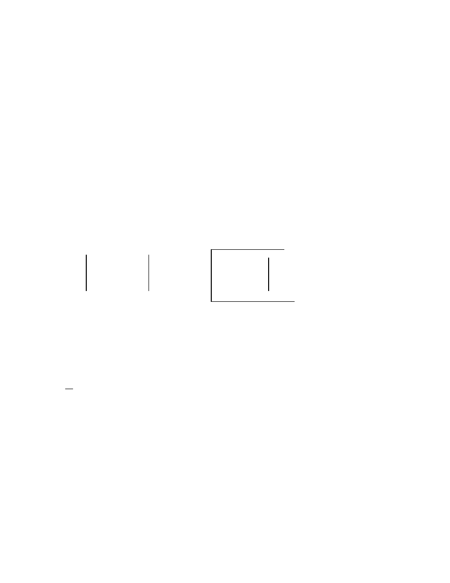
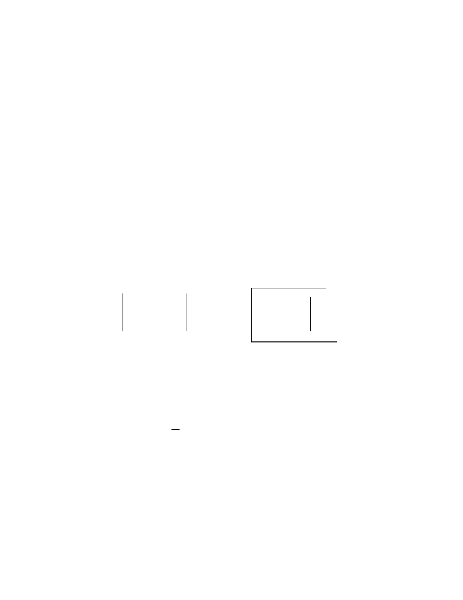
Figure 1.3:
Polyhedra can be unbounded (a) or without interior points (b). In
some books the term ‘polytope’ is reserved for bounded polyhedra with interior
points (c); we prefer to use it for all bounded polyhedra, so that (b) is a polytope
in our sense.
A polyhedral set , or polyhedron in
AR
n
is the intersection of the finite
number of closed half spaces. Since half spaces are convex, every polyhe-
dron is convex. Bounded polyhedra are called polytopes (Figure 1.3).
S
S
=
q
q
q
q
Figure 1.4:
A polyhedron is the union of its faces.
Let ∆ be a polyhedron represented as the intersection of closed halfs-
paces X
1
, . . . , X
m
bounded by the hyperplanes H
1
, . . . , H
m
. Consider the
hyperplane configuration Σ = { H
1
, . . . , H
m
}. If F is a face of Σ and has a
point in common with ∆ then F belongs to ∆. Thus ∆ is a union of faces.
Actually it can be shown that ∆ is the closure of exactly one face of Σ.
0-dimensional faces of ∆ are called vertices, 1-dimensional edges.
The following result is probably the most important theorem about
polytopes.
Theorem 1.3.1 A polytope is the convex hull of its vertices. Vice versa,
given a finite set E of points in
AR
n
, their convex hull is a polytope whose
vertices belong to E.
A. & A. Borovik • Mirrors and Reflections • Version 01 • 25.02.00
13
As R. T. Rockafellar characterised it [Roc, p. 171],
This classical result is an outstanding example of a fact which is a
completely obvious to geometric intuition, but which wields impor-
tant algebraic content and not trivial to prove.
We hope this quotation is a sufficient justification for our decision not
include the proof of the theorem in our book.
Exercises
1.3.1 Let ∆ be a tetrahedron in
AR
3
and Σ the arrangement formed by the
planes containing facets of ∆. Make a sketch analogous to Figure 1.2. Find
the number of chambers of Σ. Can you see a natural correspondence between
chambers of Σ and faces of ∆?
Hint: When answering the second question, consider first the 2-dimensional
case, Figure 1.2.
A
A
A
A
A
A
U
6
1
D
D
D
D
D
D
D
D
D
D
Q
Q
Q
Q
Q
Q
x
1
x
2
x
3
(1, 0, 0)
(0, 1, 0)
(0, 0, 1)
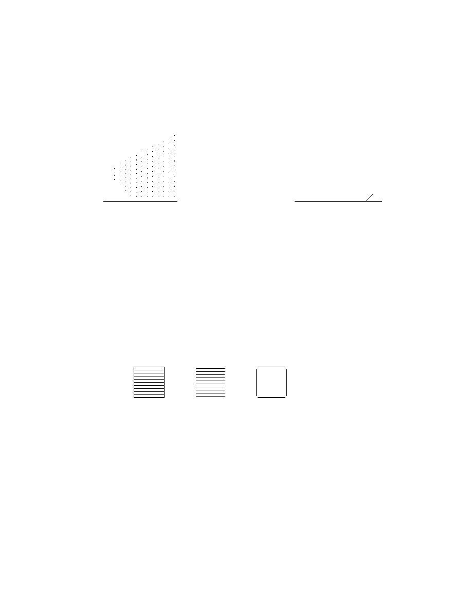
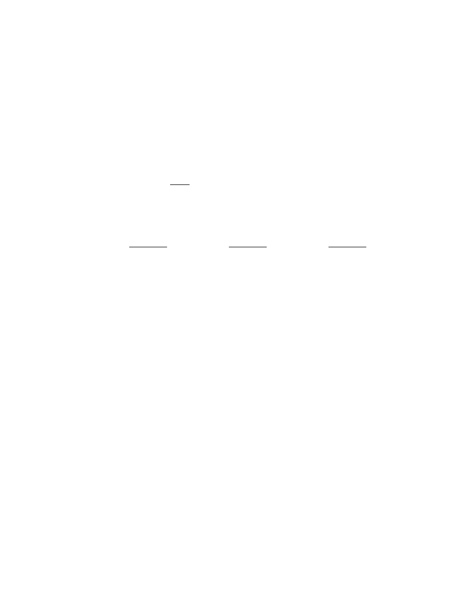
The regular 2-simplex is the set of solu-
tions of the system of simultaneous in-
equalities and equation
x
1
+ x
2
+ x
3
= 0,
x
1
> 0, x
2
> 0, x
3
> 0.
We see that it is an equilateral triangle.
Figure 1.5: The regular 2-simplex
1.3.2 The previous exercise can be generalised to the case of n dimensions in
the following way. By definition, the regular n-simplex is the set of solutions of
the system of simultaneous inequalities and equation
x
1
+ · · · + x
n
+ x
n+1
=
1
x
1
> 0
..
.
x
n+1
> 0.

14
It is the polytope in the n-dimensional affine subspace A with the equation
x
1
+· · ·+x
n+1
= 1 bounded by the coordinate hyperplanes x
i
= 0, i = 1, . . . , n+1
(Figure 1.5). Prove that these hyperplanes cut A into 2
n+1
− 1 chambers.
Hint: For a point x = (x
1
, . . . , x
n+1
) in A which does not belong to any of
the hyperplanes x
i
= 0, look at all possible combinations of the signs + and −
of the coordinates x
i
of x i = 1, . . . , n + 1.
1.4
Isometries of
AR
n
Now let us look at the structure of
AR
n
as a metric space with the distance
r(a, b) = | ~
ab|. An isometry of AR
n
is a map s from
AR
n
onto
AR
n
which
preserves the distance,
r(sa, sb) = r(a, b) for all a, b ∈ AR
n
.
We denote the group of all isometries of
AR
n
by Isom
AR
n
.
1.4.1
Fixed points of groups of isometries
The following simple result will be used later in the case of finite groups of
isometries.
Theorem 1.4.1 Let W < Isom
AR
n
be a group of isometries of
AR
n
.
Assume that, for some point e ∈ AR
n
, the orbit
W · e = { we | w ∈ W }
is finite. Then W fixes a point in
AR
n
.
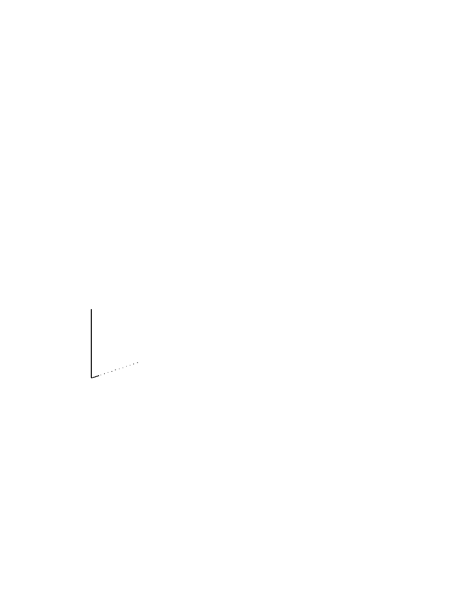
C
C
C
C
C
C
C
C
a
b
c
d
In the triangle abc the seg-
ment cd is shorter than at
least one of the sides ac or bc.
Figure 1.6: For the proof of Theorem 1.4.1
Proof
3
.
We shall use a very elementary property of triangles stated in
Figure 1.6; its proof is left to the reader.
3
This proof is a modification of a fixed point theorem for a group acting on a space
with a hyperbolic metric. J. Tits in one of his talks has attributed the proof to J. P. Serre.

A. & A. Borovik • Mirrors and Reflections • Version 01 • 25.02.00
15
Denote E = W · e. For any point x ∈ AR
n
set
m(x) = max
f ∈E
r(x, f ).
Take the point a where m(x) reaches its minimum
4
. I claim that the point
a is unique.
Proof of the claim. Indeed, if b
6= a is another minimal point, take
an inner point d of the segment [a, b] and after that a point c such that
r(d, c) = m(d). We see from Figure 1.6 that, for one of the points a and b,
say a,
m(d) = r(d, c) < r(a, c)
6 m(a),
which contradicts to the minimal choice of a.
So we can return to the proof of the theorem. Since the group W
permutes the points in E and preserves the distances in
AR
n
, it preserves
the function m(x), i.e. m(wx) = m(x) for all w ∈ W and x ∈ AR
n
, and
thus W should fix a (unique) point where the function m(x) attains its
minimum.
1.4.2
Structure of Isom
AR
n
Translations.
For every vector α ∈ R
n
one can define the map
t
α
:
AR
n
−→ AR
n
,
a
7→
a + α.
The map t
α
is an isometry of
AR
n
; it is called the translation through the
vector α. Translations of
AR
n
form a commutative group which we shall
denote by the same symbol
R
n
as the corresponding vector space.
Orthogonal transformations.
When we fix an orthonormal coordinate
system in
AR
n
with the origin o, a point a ∈ AR
n
can be identified with
its position vector α = ~
oa. This allows us to identify
AR
n
and
R
n
. Every
orthogonal linear transformation w of the Euclidean vector space
R
n
, can
4
The existence of the minimum is intuitively clear; an accurate proof consists of the
following two observations. Firstly, the function m(x), being the supremum of finite
number of continuous functions r(x, f ), is itself continuous. Secondly, we can search for
the minimum not all over the space
AR
n
, but only over the set
{ x | r(x, f) 6 m(a) for all f ∈ E },
for some a ∈ AR
n
. This set is closed and bounded, hence compact. But a continuous
function on a compact set reaches its extreme values.

16
be treated as a transformation of the affine space
AR
n
. Moreover, this
transformation is an isometry because, by the definition of an orthogonal
transformation w, (wα, wα) = (α, α), hence |wα| = |α| for all α ∈ R
n
.
Therefore we have, for α = ~
oa and β = ~
ob,
r(wa, wb) = |wβ − wα| = |w(β − α)| = |β − α| = r(a, b).
The group of all orthogonal linear transformations of
R
n
is called the or-
thogonal group and denoted
O
n
.
Theorem 1.4.2 The group of all isometries of
AR
n
which fix the point o
coincides with the orthogonal group
O
n
.
Proof.
Let s be an isometry of
AR
n
which fixes the origin o. We have
to prove that, when we treat w as a map from
R
n
to
R
n
, the following
conditions are satisfied: for all α, β ∈ R
n
,
• s(kα) = k · sα for any constant k ∈ R;
• s(α + β) = sα + sβ;
• (sα, sβ) = (α, β).
If a and b are two points in
AR
n
then, by Exercise 1.4.3, the segment
[a, b] can be characterised as the set of all points x such that
r(a, b) = r(a, x) + r(x, b).
So the terminal point a
0
of the vector cα for k > 1 is the only point
satisfying the conditions
r(o, a
0
) = k · r(0, a)
and
r(o, a) + r(a, a
0
) = r(o, a
0
).
If now sa = b then, since the isometry s preserves the distances and fixes
the origin o, the point b
0
= sa
0
is the only point in
AR
n
satisfying
r(o, b
0
) = k · r(0, b)
and
r(o, b) + r(b, b
0
) = r(o, b
0
).
Hence s · kα = ~
ob
0
= kβ = k · sα for k > 0. The cases k 6 0 and 0 < k 6 1
require only minor adjustments in the above proof and are left to the reader
as an execise. Thus s preserves multiplication by scalars.
The additivity of s, i.e. the property s(α + β) = sα + sβ, follows, in
an analogous way, from the observation that the vector δ = α + β can
be constructed in two steps: starting with the terminal points a and b of

A. & A. Borovik • Mirrors and Reflections • Version 01 • 25.02.00
17
the vectors α and β, we first find the midpoint of the segment [a, b] as the
unique point c such that
r(a, c) = r(c, b) =
1
2
r(a, b),
and then set δ = 2 ~
oc. A detailed justification of this construction is left to
the reader as an exercise.
Since s preserves distances, it preserves lengths of the vectors. But
from |sα| = |α| it follows that
(sα, sα) = (α, α)
for all α ∈ R
n
. Now we apply the additivity of s and observe that
((α + β), (α + β)) = (s(α + β), s(α + β))
= ((sα + sβ), (sα + sβ))
= (sα, sα) + 2(sα, sβ) + (sβ, sβ)
= (α, α) + 2(sα, sβ) + (β, β).
On the other hand,
((α + β), (α + β)) = (α, α) + 2(α, β) + (β, β).
Comparing these two equations, we see that
2(sα, sβ) = 2(α, β)
and
(sα, sβ) = (α, β).
Theorem 1.4.3 Every isometry of a real affine Euclidean space
AR
n
is a
composition of a translation and an orthogonal transformation. The group
Isom
AR
n
of all isometries of
AR
n
is a semidirect product of the group
R
n
of all translations and the orthogonal group
O
n
,
Isom
AR
n
=
R
n
o O
n
.

18
Proof
is an almost immediate corollary of the previous result. Indeed,
to comply with the definition of a semidirect product, we need to check
that
Isom
AR
n
=
R
n
· O
n
,
R
n
C Isom AR
n
,
and
R
n
∩ O
n
= 1.
If w ∈ Isom AR
n
is an arbitrary isometry, take the translation t = t
α
through the position vector α =
~
o, wo of the point wo. Then to = wo and
o = t
−1
wo. Thus the map s = t
−1
w is an isometry of
AR
n
which fixes
the origin o and, by Theorem 1.4.2, belongs to
O
n
. Hence w = ts and
Isom
AR
n
=
R
n
O
n
. Obviously
R
n
∩ O
n
= 1 and we need to check only
that
R
n
C Isom AR
n
. But this follows from the observation that, for any
orthogonal transformation s,
st
α
s
−1
= t
sα
,
(Exercise 1.4.5) and, consequently we have, for any isometry w = ts with
t ∈ R
n
and s ∈ O
n
,
wt
α
w
−1
= ts · t
α
· s
−1
t
−1
= t · t
sα
· t
−1
= t
sα
∈ R
n
.
Elations.
A map f :
AR
b
−→ AR
n
is called an elation if there is a
constant k such that, for all a, b ∈ AR
n
,
r(f (a), f (b)) = kr(a, b).
An isometry is a partial case k = 1 of elation. The constant k is called the
coefficient of the elation f .
Corollary 1.4.4 An elation of
AR
n
with the coefficient k is the composi-
tion of a translation, an orthogonal transformation and a map of the form
R
n
−→ R
n
α
7→
kα.
Proof
is an immediate consequence of Theorem 1.4.3.
Exercises
1.4.1 Prove the property of triangles in
AR
2
stated in Figure 1.6.

A. & A. Borovik • Mirrors and Reflections • Version 01 • 25.02.00
19
1.4.2 Barycentre. There is a more traditional approach to Theorem 1.4.1.
If F = { f
1
, . . . , f
k
} is a finite set of points in AR
n
, its barycentre b is a point
defined by the condition
k
X
j=1
~
bf
j
= 0.
1. Prove that a finite set F has a unique barycentre.
2. Further prove that the barycentre b is the point where the function
M (x) =
k
X
j=1
r(x, f
j
)
2
takes its minimal value. In particular, if the set F is invariant under the
action of a group W of isometries, then W fixes the barycentre b.
Hint: Introduce orthonormal coordinates x
1
, . . . , x
n
and show that the system of
equations
∂M (x)
∂x
i
= 0, i = 1, . . . , n,
is equivalent to the equation
P
k
j=1
~
xf
j
= 0, where x = (x
1
, . . . , x
k
).
1.4.3 If a and b are two points in
AR
n
then the segment [a, b] can be charac-
terised as the set of all points x such that r(a, b) = r(a, x) + r(x, b).
1.4.4 Draw a diagram illustrating the construction of α + β in the proof of
Theorem 1.4.2, and fill in the details of the proof.
1.4.5 Prove that if t
α
is a translation through the vector α and s is an orthog-
onal transformation then
st
α
s
−1
= t
sα
.
1.4.6 Prove the following generalisation of Theorem 1.4.1: if a group W <
Isom
AR
n
has a bounded orbit on
AR
n
then W fixes a point.
Elations.
1.4.7 Prove that an elation of
AR
n
preserves angles: if it sends points a, b, c
to the points a
0
, b
0
, c
0
, correspondingly, then
∠abc = ∠a
0
b
0
c
0
.
1.4.8 The group of all elations of
AR
n
is isomorphic to
R
n
o (O
n
× R
>0
) where
R
>0
is the group of positive real numbers with respect to multiplication.
1.4.9 Groups of symmetries. If ∆ ⊂ AR
n
, the group of symmetries Sym ∆
of the set ∆ consists of all isometries of
AR
n
which map ∆ onto ∆.
Give
examples of polytopes ∆ in
AR
3
such that
20
1. Sym ∆ acts transitively on the set of vertices of ∆ but is intransitive on
the set of faces;
2. Sym ∆ acts transitively on the set of faces of ∆ but is intransitive on the
set of vertices;
3. Sym ∆ is transitive on the set of edges of ∆ but is intransitive on the set
of faces.
1.5
Simplicial cones
1.5.1
Convex sets
Recall that a subset X ⊆ AR
n
is convex if it contains, with any points
x, y ∈ X, the segment [x, y] (Figure 1.7).
H
H
H
H
H
H
H
H
H
H
r
r
@
@
@
@
x
y
convex set
@
@
@
@
@
r
r
x
y
non-convex set
Figure 1.7: Convex and non-convex sets.
Obviously the intersection of a collection of convex sets is convex. Every
convex set is connected. Affine subspaces (in particular, hyperplanes) and
half spaces (open and closed) in
AR
n
are convex. If a set X is convex then
so are its closure X and interior X
◦
. If Y ⊆ AR
n
is a subset, it convex
hull is defined as the intersection of all convex sets containing it; it is the
smallest convex set containing Y .
1.5.2
Finitely generated cones
Cones.
A cone in
R
n
is a subset Γ closed under addition and positive
scalar multiplication, that is, α + β ∈ Γ and kα ∈ Γ for any α, β ∈ Γ and
a scalar k > 0. Linear subspaces and half spaces of
R
n
are cones. Every
cone is convex, since it contains, with any two points α and β, the segment
[α, β] = { (1 − t)α + tβ | 0 6 t 6 1 }.

A. & A. Borovik • Mirrors and Reflections • Version 01 • 25.02.00
21
A cone does not necessary contains the zero vector 0; this is the case, for
example, for the positive quadrant Γ in
R
2
,
Γ =
x
y
∈ R
2
x > 0, y > 0
.
However, we can always add to a cone the origin 0 of
R
n
: if Γ is a cone then
so is Γ ∪ { 0 }. It can be shown that if Γ is a cone then so is its topological
closure Γ and interior Γ
◦
. The intersection of a collection of cones is either
a cone or the empty set.
The cone Γ spanned or generated by a set of vectors Π is the set of all
non-negative linear combinations of vectors from Π,
Γ = { a
1
α
1
+ · · · + a
m
α
m
| m ∈ N, α
i
∈ Π, a
i
> 0 }.
Notice that the zero vector 0 belongs to Γ. If the set Π is finite then the
cone Γ is called finitely generated and the set Π is a system of generators
for Γ. A cone is polyhedral if it is the intersection of a finite number of
closed half spaces.
The following important result can be found in most books on Linear
Programming. In this book we shall prove only a very restricted special
case, Proposition 1.5.6 below.
Theorem 1.5.1 A cone is finitely generated if and only if it is polyhedral.
Extreme vectors and edges.
We shall call a set of vectors Π positive
if, for some linear functional f :
R
n
−→ R, f(ρ) > 0 for all ρ ∈ Π r { 0 }.
This is equivalent to saying that the set Π
r { 0 } of non-zero vectors in Π
is contained in an open half space. The following property of positive sets
of vectors is fairly obvious.
Lemma 1.5.2 If α
1
, . . . , α
m
are non-zero vectors in a positive set Π and
a
1
α
1
+ · · · + a
m
α
m
= 0, where all a
i
> 0,
then a
i
= 0 for all i = 1, . . . , m.
Positive cones are usually called pointed cones (Figure 1.8).
Let Γ be a cone in
R
n
. We shall say that a vector ∈ Γ is extreme
or simple in Γ if it cannot be represented as a positive linear combination
which involves vectors in Γ non-collinear to , i.e. if it follows from =
c
1
γ
1
+ · · · + c
m
γ
m
where γ
i
∈ Γ and c
i
> 0 that m = 1 and = c
1
γ
1
. Notice
that it immediately follows from the definition that if is an extreme vector
22
A
A
A
K
@
@
@
@
@
I
H
H
H
H
HH
@
@
@
:
9
I
H
H
H
H
HH
H
H
H
H
H
H
H
H
H
H
HH
H
H
H
H
H
a pointed finitely generated cone
a non-pointed finitely generated cone
Figure 1.8: Pointed and non-pointed cones
A
A
A
K
@
@
@
@
@
I
6
H
H
H
H
HH
H
H
H
H
HH
H
H
H
H
H
H
α
β
1
β
2
β
3
β
4
Γ
α is a non-extreme vector in the
cone Γ generated by extreme
(or simple) vectors β
1
, β
2
, β
3
, β
4
directed along the edges of Γ.
Figure 1.9: Extreme and non-extreme vectors.
and Π a system of generators in Γ then Π contains a vector k collinear to
.
Extreme vectors in a polyhedral cone Γ ⊂ R
2
or
R
3
have the most
natural geometric interpretation: these are vectors directed along the edges
of Γ. We prefer to take this property for the definition of an edge: if is
an extreme vector in a polyhedral cone Γ then the cone Γ ∩ R is called an
edge of Γ, see Figure 1.9.
1.5.3
Simple systems of generators
A finite system Π of generators in a cone Γ is said to be simple if it consists
of simple vectors and no two distinct vectors in Π are collinear. It follows
from the definition of an extreme vector that any two simple systems Π
and Π
0
in Γ contain equal number of vectors; moreover, every vector in Π
is collinear to some vector in Π
0
, and vice versa.
Proposition 1.5.3 Let Π be finite positive set of vectors and Γ the cone

A. & A. Borovik • Mirrors and Reflections • Version 01 • 25.02.00
23
it generates. Assume also that Π contains no collinear vectors, that is,
α = kβ for distinct vectors α, β ∈ Π and k ∈ R implies k = 0. Then Π
contains a (unique) simple system of generators.
In geometric terms this means that a finitely generated pointed cone
has finitely many edges and is generated by a system of vectors directed
along the edges, one vector from each edge.
Proof.
We shall prove the following claim which makes the statement of
the lemma obvious.
A non-extreme vector can be removed from any generating set
for a pointed cone Γ. In more precise terms, if the vectors
α, β
1
, . . . , β
k
of Π generate Γ and α is not an extreme vector
then the vectors β
1
, . . . , β
k
still generate Γ.
Proof of the claim.
Let
Π = { α, β
1
, . . . , β
k
, γ
1
, . . . , γ
l
},
where no γ
j
is collinear with α. Since α is not an extreme vector,
α =
k
X
i=1
b
i
β
i
+
l
X
j=1
c
j
γ
j
,
b
i
> 0, c
l
> 0.
Also, since the vectors α, β
1
, . . . , β
k
generate the cone Γ,
γ
j
= d
j
α +
k
X
i=1
f
ji
β
i
,
d
j
> 0, f
ji
> 0.
Substituting γ
i
from the latter equations into the former, we have, after a
simple rearrangement,
1 −
l
X
j=1
c
j
d
j
!
α =
k
X
i=1
b
i
+
l
X
j=1
c
j
f
ji
!
β
i
.
The vector α and the vector on the right hand side of this equation both
lie in the same open half space; therefore, in view of Lemma 1.5.2,
1 −
l
X
j=1
c
j
d
j
> 0
24
and
α =
1
1 −
P
j
c
j
d
j
k
X
i=1
b
i
+
l
X
j=1
c
j
f
ji
!
β
i
expresses α as a nonnegative linear combination of β
i
’s. Since the vectors
α, β
1
, . . . , β
k
generate Γ, the vectors β
1
, . . . , β
k
also generate Γ.
The following simple lemma has even simpler geometric interpretation:
the plane passing through two edges of a cone cuts in it the cone spanned
by these two edges, see Figure 1.10.
A
A
A
A
A
A
K
@
@
@
H
H
H
H
HH
α
β
Γ
The intersection of a cone Γ with the
plane spanned by two simple vectors
α and β is the coned generated by α
and β.
Figure 1.10: For the proof of Lemma 1.5.4
Lemma 1.5.4 Let α and β be two distinct extreme vectors in a finitely
generated cone Γ. Let P be the plane (2-dimensional vector subspace)
spanned by α and β. Then Γ
0
= Γ ∩ P is the cone in P spanned by α and
β.
Proof.
Assume the contrary; let γ ∈ Γ
0
be a vector which does not
belong to the cone spanned by α and β. Since α and β form a basis in the
vector space P ,
γ = a
0
α + b
0
β,
and by our assumption one of the coefficients a
0
or b
0
is negative. We can
assume without loss of generality that b
0
< 0.
Let α, β, γ
1
, . . . , γ
m
be the simple system in Γ. Since γ ∈ Γ,
γ = aα + bβ + c
1
γ
1
+ · · · + c
m
γ
m
,
where all the coefficients a, b, c
1
, . . . , c
m
are non-negative. Comparing the
two expressions for γ, we have
(a − a
0
)α + (b − b
0
)β + c
1
γ
1
+ · · · + c
m
γ
m
= 0.

A. & A. Borovik • Mirrors and Reflections • Version 01 • 25.02.00
25
Notice that b − b
0
> 0; if a − a
0
> 0 then we get a contradiction with the
assumption that the cone Γ is pointed. Therefore a − a
0
< 0 and
α =
1
a
0
− a
((b − b
0
)β + c
1
γ
1
+ · · · + c
m
γ
m
)
expresses α as a non-negative linear combination of the rest of the simple
system. This contradiction proves the lemma.
1.5.4
Duality
If Γ is a cone, the dual cone Γ
∗
is the set
Γ
∗
= { χ ∈ R
n
| (χ, γ) 6 0 for all γ ∈ Γ }.
It immediately follows from this definition that the set Γ
∗
is closed with
respect to addition and multiplication by positive scalars, so the name
‘cone’ for it is justified. Also, the dual cone Γ
∗
, being the interesection of
closed half-spaces (χ, γ)
6 0, is closed in topological sense.
The following theorem plays an extremely important role in several
branches of Mathematics: Linear Progamming, Functional Analysis, Con-
vex Geometry. We shall not use or prove it in its full generality, proving
instead a simpler partial case.
Theorem 1.5.5 (The Duality Theorem for Polyhedral Cones) If Γ is a
polyhedral cone, then so is Γ
∗
. Moreover, (Γ
∗
)
∗
= Γ.
Recall that polyhedral cones are closed by definition.
1.5.5
Duality for simplicial cones
Simplicial cones.
A finitely generated cone Γ ⊂ R
n
is called simplicial
if it is spanned by n linearly independent vectors ρ
1
, . . . , ρ
n
. Denote Π =
{ ρ
1
, . . . , ρ
n
}.
We shall prove the Duality Theorem 1.5.5 in the special case of simpli-
cial cones, and obtain, in the course of the proof, very detailed information
about their structure.
First of all, notice that if the cone Γ is generated by a finite set Π =
{ ρ
1
, . . . , ρ
n
} then the inequalities
(χ, γ)
6 0 for all γ ∈ Γ
are equivalent to
(χ, ρ
i
)
6 0, i = 1, . . . , n.
26
Hence the dual cone Γ
∗
is the intersection of the closed subspaces given by
the inequalities
(χ, ρ
i
)
6 0, i = 1, . . . , n.
We know from Linear Algebra that the conditions
(ρ
∗
i
, ρ
j
) =
−1
if i = j
0
if i 6= j
uniquely determine n linearly independent vectors ρ
∗
1
, . . . , ρ
∗
n
(see Exer-
cises 1.5.2 and 1.5.3). We shall say that the basis Π
∗
= { ρ
∗
1
, . . . , ρ
∗
n
} is
dual
5
to the basis ρ
1
, . . . , ρ
n
. If we write a vector χ ∈ R
n
in the basis Π
∗
,
χ = y
∗
1
ρ
∗
1
+ · · · + y
∗
n
ρ
∗
n
,
then (χ, ρ
i
) = −y
∗
i
and χ ∈ Γ
∗
if and only if y
i
> 0 for all i, which
means that χ ∈ Γ
∗
. So we proved the following partial case of the Duality
Theorem, illustrated by Figure 1.11.
C
C
C
C
C
C
PP
PP
PP
PPP
A
A
A
A
A
A
X
X
X
X
X
X
X
X
X
X
X
X
XXX
o
a
a
0
b
b
0
c
c
0
Γ
Γ
∗
The simplicial cones Γ and
Γ
∗
are dual to each other:
oa ⊥ b
0
oc
0
, ob ⊥ c
0
oa
0
, oc ⊥ a
0
ob
0
,
oa
0
⊥ boc, ob
0
⊥ coa, oc
0
⊥ aob.
Figure 1.11: Dual simplicial cones.
Proposition 1.5.6 If Γ is the simplicial cone spanned by a basis Π of
R
n
then the dual cone Γ
∗
is also simplicial and spanned by the dual basis Π
∗
.
Applying this property to Γ
∗
we see that Γ = (Γ
∗
)
∗
is the dual cone to Γ
∗
and coincides with the intersection of the closed half spaces
(χ, ρ
∗
i
)
6 0, i = 1, . . . , n.
5
We move a little bit away from the traditional terminology, since the dual basis is
usually defined by the conditions
(ρ
∗
i
, ρ
j
) =
1
if i = j
0
if i 6= j
.

A. & A. Borovik • Mirrors and Reflections • Version 01 • 25.02.00
27
1.5.6
Faces of a simplicial cone
Denote by H
i
the hyperplane (χ, ρ
∗
i
) = 0. Notice that the cone Γ lies in
one closed half space determined by H
i
. The intersection Γ
k
= Γ ∩ H
k
consists of all vectors of the form χ = y
1
ρ
1
+ · · · + y
n
ρ
n
with non-negative
coordinates y
i
, i = 1, . . . , n, and zero k-th coordinate, y
k
= 0. Therefore
Γ
k
is the simplicial cone in the n − 1-dimensional vector space (χ, ρ
∗
k
) = 0
spanned by the vectors ρ
i
, i 6= k. The cones Γ
k
are called facets or (n − 1)-
dimensional faces of Γ.
More generally, if we denote I = { 1, . . . , n } and take a subset J ⊂ I of
cardinality m, then the (n − m)-dimensional face Γ
J
of Γ can be defined
in two equivalent ways:
• Γ
J
is the cone spanned by the vectors ρ
i
, i ∈ I r J.
• Γ
J
= Γ ∩
T
j∈J
H
j
.
It follows from their definition that edges are 1-dimensional faces.
If we define the faces Γ
∗
J
in an analogous way then we have the formula
Γ
∗
J
= { χ ∈ Γ
∗
| (χ, γ) = 0 for all γ ∈ Γ
I
rJ
}.
Abusing terminology, we shall say that the face Γ
∗
J
of Γ
∗
is dual to the face
Γ
I
rJ
of Γ. This defines a one-to-one correspondence between the faces of
the simplicial cone Γ and its dual Γ
∗
.
In particular, the edges of Γ are dual to facets of Γ
∗
, and the facets of
Γ are dual to edges of Γ
∗
.
We shall use also the Duality Theorem for cones Γ spanned by m < n
linearly independent vectors in
R
n
. The description of Γ
∗
in this case is an
easy generalisation of Proposition 1.5.6; see Exercise 1.5.4.
Exercises
1.5.1 Let X be an arbitrary positive set of vectors in
R
n
. Prove that the set
X
∗
= { α ∈ R
n
| (α, γ) 6 0 }
is a cone. Show next that X
∗
contains a non-zero vector and that X is contained
in the cone (X
∗
)
∗
.
1.5.2 Dual basis. Let
1
, . . . ,
n
be an orthonormal basis and ρ
1
, . . . , ρ
n
a
basis in
R
n
. Form the matrix R = (r
ij
) by the rule r
ij
= (ρ
i
,
j
), so that ρ
i
=
P
n
j=1
r
ij
j
. Notice that R is a non-degenerate matrix. Let ρ = y
1
1
+ · · · + y
n
n
.
For each value of i, express the system of simultaneous equations
(ρ, ρ
j
) =
−1
if i = j
0
if i 6= j
28
in matrix form and prove that it has a unique solution. This will prove the
existence of the basis dual to ρ
1
, . . . , ρ
n
.
1.5.3 A formula for the dual basis. In notation of Exercise 1.5.2, prove
that the dual basis { ρ
∗
i
} can be determined from the formula
ρ
∗
j
= −
1
det R
r
11
. . .
r
1,j−1
1
r
1,j+1
. . .
r
1,n
r
21
. . .
r
2,j−1
2
r
2,j+1
. . .
r
2,n
..
.
..
.
..
.
..
.
..
.
r
i,1
. . .
r
i,j−1
i
r
i,j+1
. . .
r
i,n
..
.
..
.
..
.
..
.
..
.
r
n,1
. . .
r
n,j−1
n
r
n,j+1
. . .
r
n,n
.
Notice that in the case n = 3 we come to the formula
ρ
∗
1
= −
1
(ρ
1
, ρ
2
, ρ
3
)
ρ
2
×ρ
3
,
ρ
∗
2
= −
1
(ρ
1
, ρ
2
, ρ
3
)
ρ
3
×ρ
1
,
ρ
∗
3
= −
1
(ρ
1
, ρ
2
, ρ
3
)
ρ
1
×ρ
2
,
where ( , , ) denotes the scalar triple product and × the cross (or vector)
product of vectors.
1.5.4 Let Γ be a cone in
R
n
spanned by a set Π of m linearly independent
vectors ρ
1
, . . . , ρ
m
, with m < n. Let U be the vector subspace spanned by Π.
Then Γ is a simplicial cone in U ; we denote its dual in U as Γ
0
, and set Γ
∗
to be the dual cone for Γ in V . Let also Π
0
= { ρ
0
1
, . . . , ρ
0
m
} be the basis in U
dual to the basis Π. We shall use in the sequel the following properties of the
cone Γ
∗
.
1. For any set A ∈ R
n
, define
A
⊥
= { χ ∈ R
n
| (χ, α) = 0 for all γ ∈ A }.
Check that A
⊥
is a linear subspace of
R
n
. Prove that dim Γ
⊥
= n − m.
Hint: Γ
⊥
= U
⊥
.
2. Γ
∗
is the intersection of the closed half spaces defined by the inequalities
(χ, ρ
i
)
6 0, i = 1, . . . , m.
3. Γ
∗
= Γ
0
+ Γ
⊥
; this set is, by definition,
Γ
0
+ Γ
⊥
= { κ + χ | κ ∈ Γ
0
, χ ∈ Γ
⊥
}.
4. (Γ
∗
)
∗
= Γ.
5. Let H
i
and H
∗
i
be the hyperplanes in V given by the equations (χ, ρ
0
i
) = 0
and (χ, ρ
i
) = 0, correspondingly. Denote I = { 1, . . . , m } and set, for
J ⊆ I,
Γ
J
= Γ ∩
\
j∈J
H
j
, Γ
∗
J
= Γ
∗
∩
\
j∈J
H
∗
j
and Γ
0
J
= Γ
0
∩
\
j∈J
H
∗
j
.
Prove that Γ
∗
J
= Γ
0
J
+ Γ
⊥
.

A. & A. Borovik • Mirrors and Reflections • Version 01 • 25.02.00
29
6. The cones Γ
J
and Γ
∗
J
are called faces of the cones Γ and Γ
∗
, corre-
spondingly. There is a one-to-one correspondence between the set of k-
dimensional faces of Γ, k = 1, . . . , m−1, and n−k dimensional faces of Γ
∗
,
defined by the rule Γ
∗
J
= Γ ∩ Γ
⊥
I
rJ
. If we treat Γ as its own m-dimensional
face Γ
∅
, then it corresponds to Γ
∗
I
= Γ
⊥
.

30

Chapter 2
Mirrors, Reflections, Roots
2.1
Mirrors and reflections
Mirrors and reflections.
Recall that a reflection in an affine real Eu-
clidean space
AR
n
is a nonidentity isometry s which fixes all points of
some affine hyperplane (i.e. affine subspace of codimension 1) H of
AR
n
.
The hyperplane H is called the mirror of the reflection s and denoted H
s
.
Conversely, the reflection s will be sometimes denoted as s = s
H
.
Lemma 2.1.1 If s is a reflection with the mirror H then, for any point
α ∈ AR
n
,
• the segment [sα, α] is normal to H and H intersects the segment in
its midpoint;
• H is the set of points fixed by s;
• s is an involutary transformation
1
, that is, s
2
= 1.
In particular, the reflection s is uniquily determined by its mirror H, and
vice versa.
Proof.
Choose some point of H for the origin o of a orthonormal coor-
dinate system, and identify the affine space
AR
n
with the underlying real
Euclidean vector space
R
n
. Then, by Theorem 1.4.2, s can be identified
with an orthogonal transformation of
R
n
. Since s fixes all points in H, it
has at least n − 1 eigenvalues 1, and, since s is non identity, the only possi-
bility for the remaining eigenvalue is −1. In particular, s is diagonalisable
and has order 2, that is s
2
= 1 and s 6= 1. It also follows from here that H
is the set of all point fixed by s.
1
A non-identity element g of a group G is called an involution if it has order 2. Hence
s is an involution.
31
32
t
t
t
t
t
t
b
b
b
b
b
b
b
bb
b
b
b
b
bb
b
b
b
b
b
b
b
b
b
b
b
tα
α
H
sα
tH
t
t
t
s
0
tα = tsα
Figure 2.1:
For the proof of Lemma 2.1.3: If s is the reflection in the mirror H
and t is an isometry then the reflection s
0
in the mirror tH can be found from
the condition s
0
t = ts hence s
0
= tst
−1
.
If now we consider the vector sα − α directed along the segment [sα, α]
then
s(sα − α) = s
2
α − sα = α − sα,
which means that the vector sα −α is an eigenvector of s for the eigenvalue
−1. Hence the segment [sα, α] is normal to H. Its midpoint
1
2
(sα + α) is
s-invariant, since
s
1
2
(sα + α) =
1
2
(s
2
α + sα) =
1
2
(sα + α),
hence belongs to H.
In the course of the proof of the previous lemma we have also shown
Lemma 2.1.2 Reflections in
AR
n
which fix the origin o are exactly the or-
thogonal transformations of
R
n
with n−1 eigenvalues 1 and one eigenvalue
−1; their mirrors are eigenspaces for the eigenvalue 1.
We say that the points sα and α are symmetric in H. If X ⊂ A then
the set sX is called the reflection or the mirror image of the set X in the
mirror H.
Lemma 2.1.3 If t is an isometry of
AR
n
, s the reflection in the mirror
H and s
0
is the reflection in tH then s
0
= tst
−1
.

A. & A. Borovik • Mirrors and Reflections • Version 01 • 25.02.00
33
Proof.
See Figure 2.1. Alternatively, we may argue as follows.
We need only show that tst
−1
is a non-identity isometry which fixes
tH. Since tst
−1
is a composition of isometries, it is clearly an isometry. If
α ∈ tH, then t
−1
α ∈ H, hence s fixes t
−1
α, hence tst
−1
α = α. If α 6∈ tH,
then t
−1
α 6∈ H, hence s does not fix t
−1
α, hence tst
−1
α 6= α.
Exercises
Reflections and rotations in
R
2
.
2.1.1 Prove that every 2 orthogonal matrix A over
R can be written in one of
the forms
cos θ
− sin θ
sin θ
cos θ
or
cos θ
sin θ
sin θ
− cos θ
,
depending on whether A has determinant 1 or −1.
2.1.2 Prove that if, in the notation of the previous Exercise, det A = 1 then A is
the matrix of the rotation through the angle θ about the origin, counterclockwise.
2.1.3 Prove that if det A = −1 then A is the matrix of a reflection.
2.1.4 Check that
u =
cos φ/2
sin φ/2
and v =
− sin φ/2
cos φ/2
are eigenvectors with the eigenvalues 1 and −1 for the matrix
cos φ
sin φ
sin φ
− cos φ
.
2.1.5 Use trigonometric identities to prove that
cos φ
− sin φ
sin φ
cos φ
·
cos ψ
− sin ψ
sin ψ
cos ψ
=
cos(φ + ψ)
− sin(φ + ψ)
sin(φ + ψ)
cos(φ + ψ)
.
Give a geometric interpretation of this fact.

34
Finite groups of orthogonal transformations in 2 dimensions.
2.1.6 Prove that any finite group of rotations of the Euclidean plane
R
2
about
the origin is cyclic.
Hint: It is generated by a rotation through the smallest angle.
2.1.7 Prove that if r is a rotation of
R
2
and s a reflection then sr is a reflection,
in particular, |sr| = 2. Deduce from this the fact that s inverts r, i.e. srs
−1
=
r
−1
.
2.1.8 If G is a finite group of orthogonal transformations of the 2-dimensional
Euclidean space
R
2
then the map
det : G
−→ { 1, −1 }
A
7→
det A
is a homomorphism with the kernel R consisting of all rotations contained in G.
If R 6= G then |G : R| = 2 and all elements in G r R are reflections.
2.1.9 Prove that the product of two reflections in
R
2
(with a common fixed
point at the origin) is a rotation through twice the angle between their mirrors.
Involutary orthogonal transformations in three dimensions.
2.1.10 In
R
3
there are three, up to conjugacy of matrices, involutive orthog-
onal transformations, with the eigenvalues 1, 1, −1 (reflections), 1, −1, −1 and
−1, −1, −1. Give a geometric interpretation of the two latter transformations.
2.2
Systems of mirrors
Assume now that we are given a solid ∆ ⊂ AR
n
. Consider the set Σ of all
mirrors of symmetry of ∆, i.e. the mirrors of reflections which send ∆ to
∆. The reader can easily check (Exercise 2.2.1) that Σ is a closed system
of mirrors in the sense of the following definition: a system of hyperplanes
(mirrors) in A is called closed if, for any two mirrors H
1
and H
2
in Σ, the
mirror image of H
2
in H
1
also belongs to Σ (see Figure 2.)
Slightly abusing language, we shall call a finite closed system Σ of
mirrors simply a system of mirrors.
Systems of mirrors are the most natural objects. The reader most likely
has seen them when looking into a kaleidoscope
2
; and, of course, everybody
2
My special thanks are due to Dr. Robert Sandling who lent me, for demonstration
to my students, a fascinating old fashioned kaleidoscope. It contained three mirrors
arranged as the side faces of a triangular prism with an equilateral base and produced
the mirror system of type ˜
A
2
.
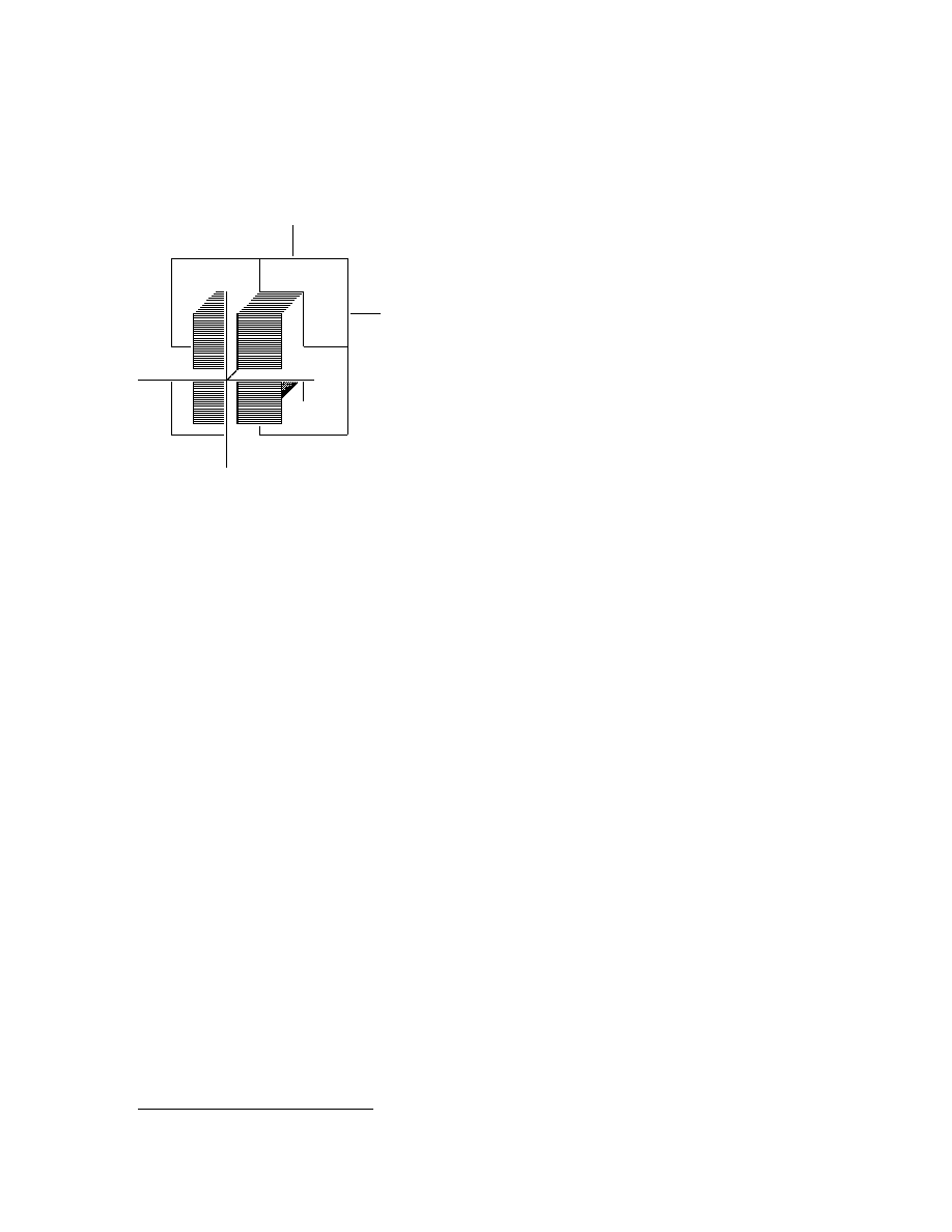
A. & A. Borovik • Mirrors and Reflections • Version 01 • 25.02.00
35
Σ
The system Σ of mirrors of
symmetry of a geometric body
∆ is closed: the reflection of a
mirror in another mirror is a
mirror again.
Notice that if
∆ is compact then all mirrors
intersect in a common point.
Figure 2.2: A closed system of mirrors.
has seen a mirror
3
. We are interested in the study of finite closed systems of
mirrors and other, closely related objects—root systems and finite groups
generated by reflections.
Systems of reflections.
If Σ is a system of mirrors, the set of all re-
flections in mirrors of Σ will be refered to as a closed system of reflections.
In view of Lemma 2.1.3, a set S of reflections forms a closed system of
reflections if and only if s
t
∈ S for all s, t ∈ S. Here s
t
is the standard, in
group theory, abbreviation for conjugation: s
t
= t
−1
st. Recall that con-
jugation by any element t is an automorphism of any group containing t:
(xy)
t
= x
t
y
t
.
Lemma 2.2.1 A finite closed system of reflections generates a finite group
of isometries.
Proof.
This result is a partial case of the following elementary group
theoretic property.
Let W be a group generated by a finite set S of involutions such
that s
t
∈ S for all s, t ∈ S. Then W is finite.
Indeed, since s ∈ S are involutions, s
−1
= s. Let w ∈ W and find the
shortest expression w = s
1
· · · s
k
of w as a product of elements from S. If
3
We cannot resist temptation and recall an old puzzle: why is it that the mirror
changes left and right but does not change up and down?
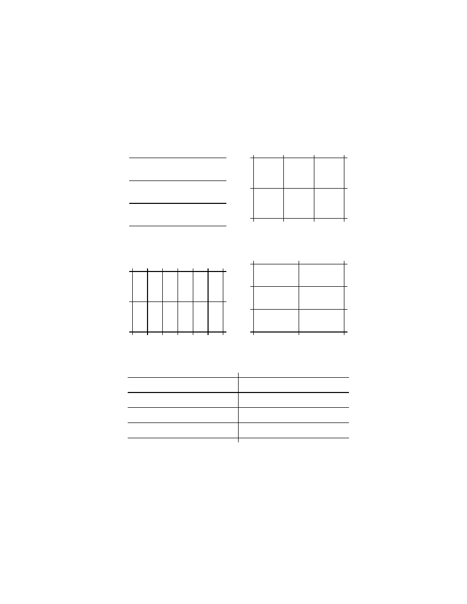
36
J
J
J
J
J
J
J
J
J
J
J
J
J
J
J
J
J
J
J
J
J
J
J
J
J
J
J
J
J
J
J
J
J
J
J
J
J
˜
A
2
@
@
@
@
@
@
@
@
@
@
@
@
@
@
@
@
@
@
@
@
@
@
@
@
@
@
@
@
g
BC
2
˜
A
1
+ ˜
A
1
J
J
H
H
H
H
H
H
H
H
H
H
H
HH
J
J
J
J
J
J
J
J
J
J
J
J
J
J
J
J
J
J
J
H
H
H
H
H
HH
J
J
J
J
J
J
J
J
J
J
J
J
J
J
J
J
˜
G
2
A
1
+ ˜
A
1
Figure 2.3:
Examples of infinite closed mirror systems in
AR
2
with their tradi-
tional notation: tesselations of the plane by congruent equilateral triangles ( ˜
A
2
),
isosceles right triangles (g
BC
2
), rectangles ( ˜
A
1
+ ˜
A
1
), triangles with the angles
π/2, π/3, π/6 ( ˜
G
2
), infinite half stripes (A
1
+ ˜
A
1
).

A. & A. Borovik • Mirrors and Reflections • Version 01 • 25.02.00
37
the word s
1
· · · s
k
contains two occurrences of the same involution s ∈ S
then
w = s
1
· · · s
i
ss
i+1
· · · s
j
ss
j+1
· · · s
k
= s
1
· · · s
i
(s
i+1
· · · s
j
)
s
s
j+1
· · · s
k
= s
1
· · · s
i
s
s
i+1
· · · s
s
j
s
j+1
· · · s
k
= s
1
· · · s
i
s
0
i+1
· · · s
0
j
s
j+1
· · · s
k
,
where all s
0
l
= s
s
l
belong to S and the resulting expression is shorter then
the original. Therefore all shortest expressions of elements from W in
terms of generators s ∈ S contain no repetition of symbols. Therefore the
length of any such expression is at most |S|, and, counting the numbers
of expressions of length 0, 1, . . . , |S|, we find that their total number is at
most
1 + |S| + |S|
2
+ · · · + |S|
|S|
.
Hence W is finite.
Finite reflection groups.
A group-theoretic interpretation of closed
systems of mirrors comes in the form of a finite reflection group, i.e. a
finite group W of isometries of an affine Euclidean space A generated by
reflections.
Let s be a reflection in W and s
W
= { wsw
−1
| w ∈ W } its conjugacy
class. Form the set of mirrors Σ = { H
t
| t ∈ s
W
}. Then it follows from
Lemma 2.1.3 that Σ is a mirror system: if H
r
, H
t
∈ Σ then the reflection
of H
r
in H
t
is the mirror H
r
t
. Thus s
W
is a closed system of reflections.
The same observation is valid for any normal set S of reflections in W ,
i.e. a set S such that s
w
∈ S for all s ∈ S and w ∈ W . We shall show
later that if the reflection group W arises from a closed system of mirrors
Σ then every reflection in W is actually the reflection in one of the mirrors
in Σ.
Since W is finite, all its orbits are finite and W fixes a point by virtue
of Theorem 1.4.1. We can take this fixed point for the origin of an or-
thonormal coordinate system and, in view of Theorem 1.4.2, treat W as a
group of linear orthogonal transformations.
If W is the group generated by the reflections in the finite closed system
of mirrors Σ then the fixed points of W are fixed by every reflection in a
mirror from Σ hence belong to each mirror in Σ. Thus we proved
Theorem 2.2.2 (1) A finite reflection group in
AR
n
has a fixed point.
(2) All the mirrors in a finite closed system of mirrors in
AR
n
have a point
in common.

38
Since we are interested in finite closed system of mirros and finite groups
generated by reflections, this result allows us to assume without loss of
generality that all mirrors pass through the origin of
R
n
. So we can forget
about the affine space
AR
n
and work entirely in the Euclidean vector space
V =
R
n
.
Exercises
Systems of mirrors.
2.2.1 Prove that if ∆ is a subset in
AR
n
then the system Σ of its mirrors of
symmetry is closed.
Hint: If M and N are two mirrors in Σ with the reflections s and t, then, in
view of Lemma 2.1.3, the mirror image of M in N is the mirror of the reflection
s
t
. If s and t map ∆ onto ∆ then so does s
t
.
"
"
"
b
b
b
b
b
b
b
b
b
b
b
bb
3
k
s v
f
Figure 2.4: Billiard, for Exercise 2.2.2.
2.2.2 Two balls, white and black, are placed on a billiard table (Figure 2.4).
The white ball must bounce off two cushions of the table and then strike the
black one. Find its trajectory.
2.2.3 Prove that a ray of light reflecting from two mirrors forming a corner will
eventually get out of the corner (Figure 2.5). If the angle formed by the mirrors
is α, what is the maximal possible number of times the ray would bounce off
the sides of the corner?
2.2.4 Prove that the angular reflector made of three pairwise perpendicular
mirrors in
R
3
sends a ray of light back in the direction exactly opposite to the
one it came from, (Figure 2.6).

A. & A. Borovik • Mirrors and Reflections • Version 01 • 25.02.00
39
PP
PP
PP
PP
PP
PP
PP
α
6
R
hhhhh
h
y
(((
(((
:
Figure 2.5: For Exercise 2.2.3.
Reflections and Linear Algebra.
2.2.5 We say that a subpace U of the real Euclidean space V is perpendicular to
the subspace W and write U ⊥ W if U = (U ∩ W ) ⊕ U
0
where U
0
is orthogonal
to W , i.e. (u, w) = 0 for all u ∈ U
0
and w ∈ W . Prove that this relation is
symmetric; U ⊥ W if and only if W ⊥ U.
2.2.6 Prove that if a reflection s leaves a subspace U < V invariant then U is
perpendicular to the mirror H
s
of the reflection s.
2.2.7 Prove that two reflections s and t commute, that is, st = ts, if and only
if their mirrors are perpendicular to each other.
Planar geometry.
2.2.8 Prove that the product of two reflections in
AR
2
with parallel mirrors is
a parallel translation. What is the translation vector?
2.2.9 If a bounded figure in the Euclidean plane
AR
2
has a center of symmetry
and a mirror of symmetry then it has two perpendicular mirrors of symmetry.
Is the same true in
AR
3
?
2.3
Dihedral groups
In this section we shall study finite groups generated by two involutions.
Theorem 2.3.1 There is a unique, up to isomorphism, group W gener-
ated by two involutions s and t such that their product st has order n.
Furthermore,
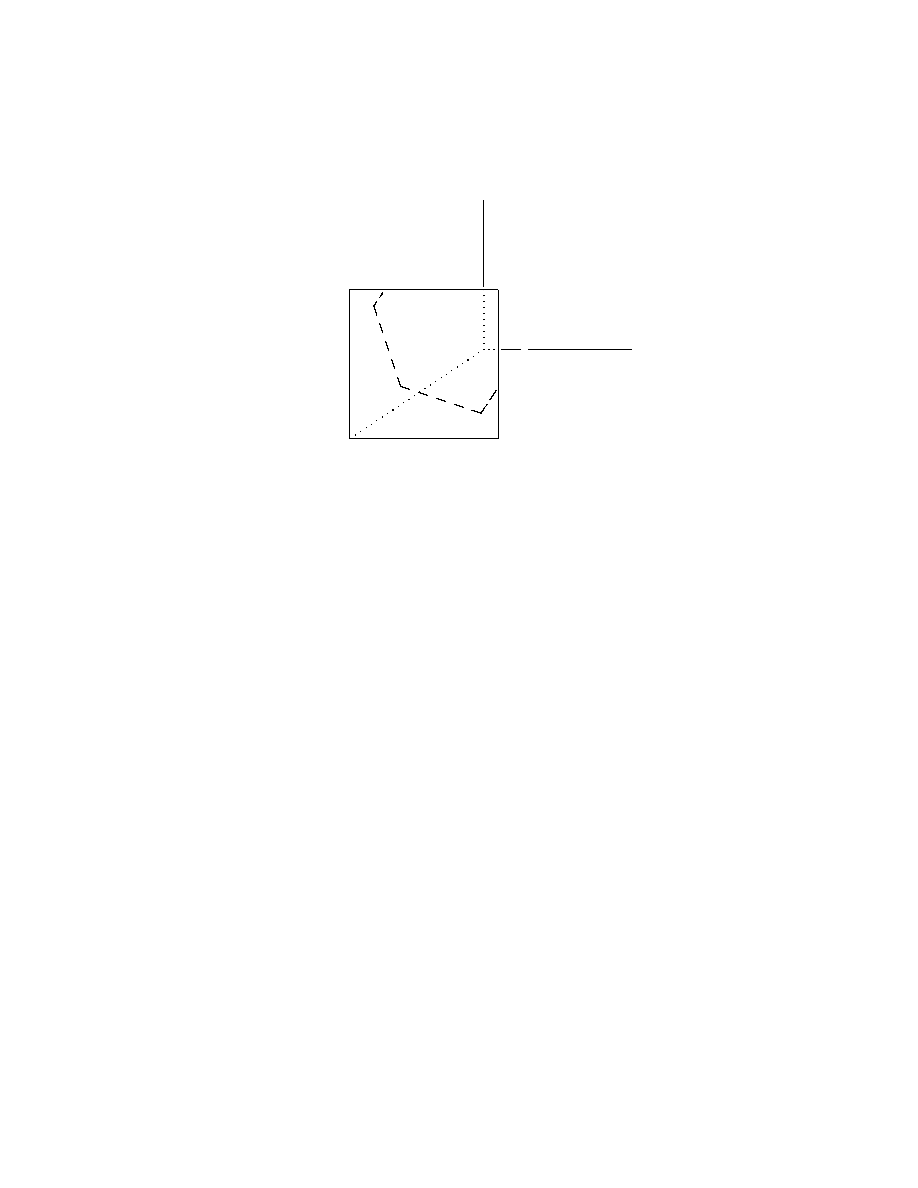
40
N
q
Figure 2.6:
Angular reflector (for Exercise 2.2.4).
(1) W is finite and |W | = 2n.
(2) If r = st then the cyclic group R = hri generated by r is a normal
subgroup of W of index 2.
(3) Every element in W
r R is an involution.
We shall denote the group W as D
2n
, call it the dihedral group of order
2n and write
D
2n
= hs, t | s
2
= t
2
= (st)
n
= 1i.
This standard group-theoretical notation means that the group D
2n
is gen-
erated by two elements s and t such that any identity relating them to each
other is a consequence of the generating relations
s
2
= 1, t
2
= 1, (st)
n
= 1.
The words ‘consequence of the generating relations’ are given precise mean-
ing in the theory of groups given by generators and relations, a very well
developed chapter of the general theory of groups. We prefer to use them
in a informal way which will be always clear from context.
Proof of the Theorem 2.3.1.
First of all, notice that, since s
2
= t
2
= 1,
s
−1
= s and t
−1
= t.

A. & A. Borovik • Mirrors and Reflections • Version 01 • 25.02.00
41
In particular, (st)
−1
= t
−1
s
−1
= ts. Set r = st. Then
r
t
= trt = t · st · t = ts = r
−1
and analogously r
s
= r
−1
.
Since s = rt, the group W is generated by r and t and every element
w in W has the form
w = r
m
1
t
k
1
· · · r
m
l
t
k
l
,
where m
i
takes the values 0, 1, . . . , n −1 and k
i
is 0 or 1. But one can check
that, since trt = r
−1
,
tr = r
−1
t,
tr
m
= r
−m
t
and
t
k
r
m
= r
(−1)
k
m
t
k
.
Hence
(r
m
1
t
k
1
)(r
m
2
t
k
2
) = r
m
t
k
(2.1)
where
k = k
1
+ k
2
, m = m
1
+ (−1)
k
1
m
2
.
Therefore every element in W can be written in the form
w = r
m
t
k
, m = 0, . . . , n − 1, k = 0, 1.
Furthemore, this presentation is unique. Indeed, assume that
r
m
1
t
k
1
= r
m
2
t
k
2
where m
1
, m
2
∈ { 0, . . . , n − 1 } and k
1
, k
2
∈ { 0, 1 }. If k
1
= k
2
then
r
m
1
= r
m
2
and m
1
= m
2
. But if k
1
6= k
2
then
r
m
1
−m
2
= t.
Denote m = m
1
− m
2
. Then m < n and r
m
= (st)
m
= t. If m = 0 then
t = 1, which contradicts to our assumption that |t| = 2. Now we can easily
get a final contradiction:
st · st · · · st = t
implies
s · ts · · · ts · · · ts = 1.
The word on the left contains an odd number of elements s and t. Consider
the element r in the very center of the word; r is either s or t. Hence the
previous equation can be rewritten as
sts · · · r · · · sts = [sts · · ·]r[sts · · ·]
−1
= 1,
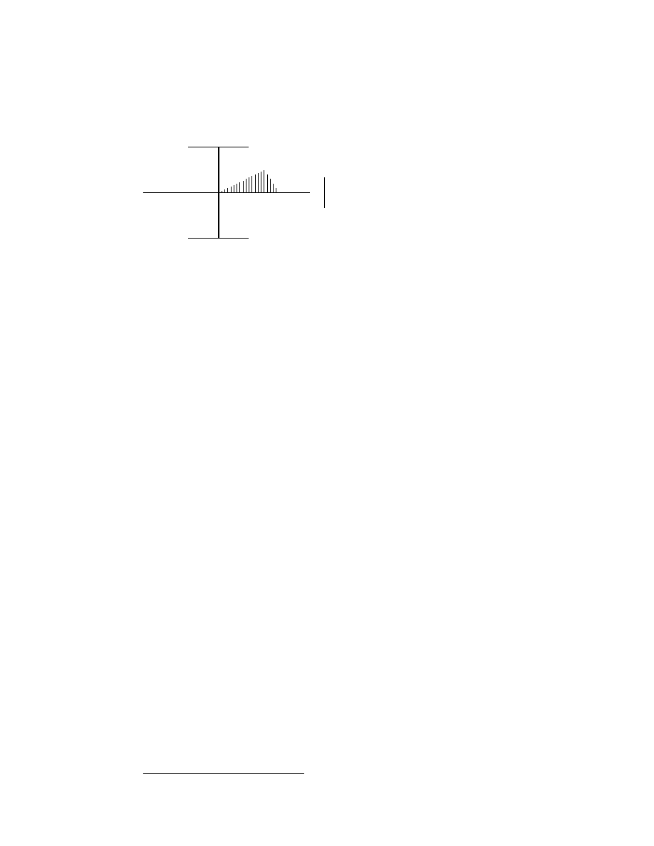
42
J
J
J
J
J
J
J
J
J
J
H
H
H
H
H
H
H
HH
J
J
J
J
J
J
J
J
J
J
J
J
]
J
J
J
^
s
6
?
t
A
B
C
The group of symmetries of the
regular n-gon ∆ is generated
by two reflections s and t in
the mirrors passing through the
midpoint and a vertex of a side
of ∆.
Figure 2.7: For the proof of Theorem 2.3.2.
which implies r = 1, a contradiction.
Since elements of w can be represented by expressions r
m
t
k
, and in a
unique way, we conclude that |W | = 2n and
W = { r
m
t
k
| m = 0, 1, . . . , n − 1, k = 0, 1 },
with the multiplication defined by Equation 2.1. This proves existence and
uniqueness of D
2n
.
Since |r| = n, the subgroup R = hri has index 2 in W and hence is
normal in W . If w ∈ W r R then w = r
m
t for some m, and a direct
computation shows
w
2
= r
m
t · r
m
t = r
−m+m
t
2
= 1.
Since w 6= 1, w is an involution.
Theorem 2.3.2 The group of symmetries Sym ∆ of the regular n-gon ∆
is isomorphic to the dihedral group D
2n
.
Proof.
Denote W = Sym ∆. The mirrors of symmetry of the polygon ∆
cut it into 2n triangle slices
4
, see Figure 2.7. Notice that any two adjacent
slices are interchanged by the reflection in their common side. Therefore
W acts transitively on the set S of all slices. Also, observe that only the
identity symmetry of ∆ maps a slice onto itself. By the well-known formula
for the length of a group orbit
|W | =
number
of slices
·
order of the
stabiliser
of a slice
= 2n · 1 = 2n.
4
Later we shall use for them the more terms fundamental regions or chambers.

A. & A. Borovik • Mirrors and Reflections • Version 01 • 25.02.00
43
Next, if s and t are reflections in the side mirrors of a slice, then their
product st is a rotation through the angle 2π/n, which can be immediately
seen from the picture: st maps
5
the vertex A to B and B to C.
By
Theorem 2.3.1, |hs, ti| = 2n; hence W = hs, ti is the dihedral group of
order 2n.
Exercises
2.3.1 Prove that the dihedral group D
6
is isomorphic to the symmetric group
Sym
3
.
2.3.2 The centre of a dihedral group. If n > 2 then
Z(D
2n
) =
{ 1 }
if n is odd,
{ 1, r
n
2
} = hr
n
2
i
if n is even.
2.3.3 Klein’s Four Group. Prove that D
4
is an abelian group,
D
4
= { 1, s, t, st }.
(It is traditionally called Klein’s Four Group.)
2.3.4 Prove that the dihedral group D
2n
, n > 2, has one class of conjugate
involutions, in n is odd, and three classes, if n is even. In the latter case, one of
the classes contains just one involution z and Z(D
2n
) = { 1, z }.
2.3.5 Prove that a finite group of orthogonal transformations of
R
2
is either
cyclic, or a dihedral group D
2n
.
2.3.6 If W = D
2n
is a dihedral group of orthogonal transformations of
R
2
,
then W has one conjugacy class of reflections, if n is odd, and two conjugacy
classes of reflections, if n is even.
2.3.7 Check that the complex numbers
e
2kπi/n
= cos 2kπ/n + i sin 2kπ/n, k = 0, 1, . . . , n − 1
in the complex plane
C are vertices of a regular n-gon ∆. Prove that the maps
r : z
7→ z · e
2πi/n
,
t : z
7→ ¯
z,
where ¯ denotes the complex conjugation, generate the group of symmetries of
∆.
2.3.8 Use the idea of the proof of Theorem ?? to find the orders of the groups
of symmetries of the regular tetrahedron, cube, dodecahedron.
5
We use ‘left’ notation for action, so when we apply the composition st of two
transformations s and t to a point, we apply t first and then s: (st)A = s(tA).

44
2.4
Root systems
Mirrors and their normal vectors.
Consider a reflection s with the
mirror H. If we choose the orthogonal system of coordinates in V with the
origin O belonging to H then s fixes O and thus can be treated as a linear
orthogonal transformation of V . Let us take a nonzero vector α perpen-
dicular to H then, obviously,
Rα = H
⊥
is the orthogonal complement of
H in V , s preserves H
⊥
and therefore sends α to −α. Then we can easily
check that s can be written in the form
s
α
β = β −
2(β, α)
(α, α)
α,
where (α, β) denotes the scalar product of α and β. Indeed, a direct com-
putation shows that the formula holds when β ∈ H and when β = α. By
the obvious linearity of the right side of the formula with respect to β, it
is also true for all β ∈ H + Rα = V .
Also we can check by a direct computation (left to the reader as an
exercise) that, given the nonzero vector α, the linear transformation s
α
is
orthogonal, i.e. (s
α
β, s
α
γ) = (β, γ) for all vectors β and γ. Finally, s
α
= s
cα
for any nonzero scalar c.
Notice that reflections can be characterized as linear orthogonal trans-
formations of
R
n
with one eigenvalue −1 and (n − 1) eigenvalues 1; the
vector α in this case is an eigenvector corresponding to the eigenvalue −1.
Thus we have a one-to-one correspondence between the three classes of
objects:
• hyperplanes (i.e. vector subspaces of codimension 1) in the Euclidean
vector space V ;
• nonzero vectors defined up to multiplication by a nonzero scalar;
• reflections in the group of orthogonal transformations of V .
The mirror H of the reflection s
α
will be denoted by H
α
. Notice that
H
α
= H
cα
for any non-zero scalar c.
Notice, finally, that orthogonal linear transformations of the Euclidean
vector space V (with the origin O fixed) preserve the relations between
mirrors, vectors and reflections.
Root systems.
Traditionally closed systems of reflections were studied
in the disguise of root systems. By definition, a finite set Φ of vectors in V
is called a root system if it satisfies the following two conditions:
(1) Φ ∩ Rρ = { ρ, −ρ } for all ρ ∈ Φ;
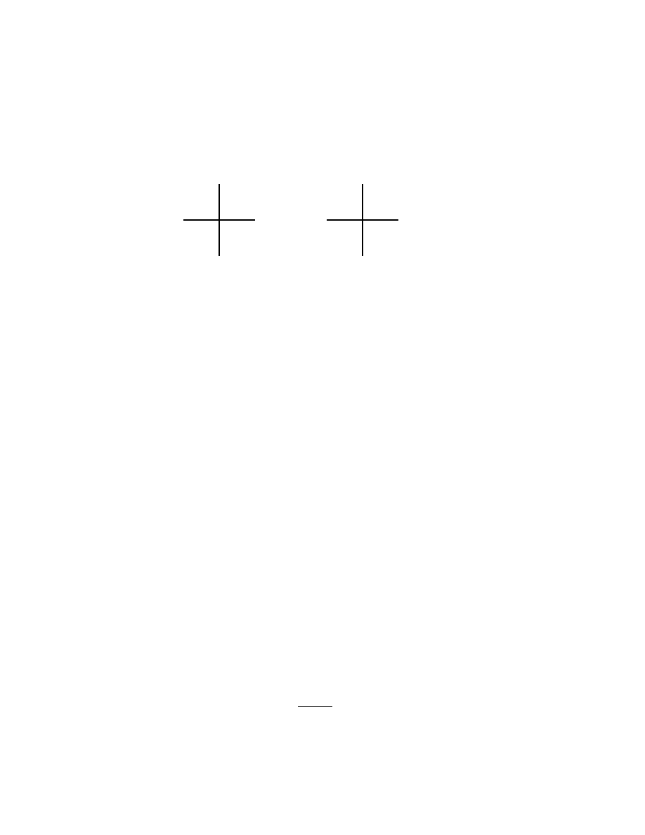
A. & A. Borovik • Mirrors and Reflections • Version 01 • 25.02.00
45
@
@
@
@
I
6
-
@
@
@
@
R
?
Φ
@
@
@
I
6
-
@
@
@
R
?
Φ
0
Figure 2.8:
If Φ is a root system then the vectors ρ/|ρ| with ρ ∈ Φ form the
root system Φ
0
with the same reflection group. We are not much interested in
lengths of roots and in most cases can assume that all roots have length 1.
(2) s
ρ
Φ = Φ for all ρ ∈ Φ.
The following lemma is an immediate corollary of Lemma 2.1.3.
Lemma 2.4.1 Let Σ be a finite closed system of mirrors. For every mirror
H in Σ take two vectors ±ρ of length 1 perpendicular to H. Then the
collection Φ of all these vectors is a root system. Vice versa, if Φ is a root
system then { H
ρ
| ρ ∈ Φ } is a system of mirrors.
Proof.
We need only to recall that a reflection s, being an orthogonal
transformation, preserves orthogonality of vectors and hyperplanes: if ρ is
a vector and H is a hyperplane then ρ ⊥ H if and only if sρ ⊥ sH.
Also we can restate Lemma 2.2.1 in terms of root systems.
Lemma 2.4.2 Let Φ be a root system. Then the group W generated by
reflections s
ρ
for ρ ∈ Φ is finite.
Exercises
2.4.1 Prove, by direct computation, that the linear transformation s
α
given
by the formula
s
α
β = β −
2(β, α)
(α, α)
α,
is orthogonal, that is,
(s
α
β, s
α
β) = (β, β)
for all β ∈ V .

46
2.4.2 Let Φ be a root system in the Euclidean space V and U < V a vector
subspace of V . Prove that Φ ∩ U is a (possibly empty) root system in U.
2.4.3 Let V
1
and V
2
be two subspaces orthogonal to each other in the real
Euclidean vector space V and Φ
i
be a root system in V
i
, i = 1, 2. Prove that
Φ = Φ
1
∪ Φ
2
is a root system in V
1
⊕ V
2
; it is called the direct sum of Φ
1
and Φ
2
and denoted
Φ = Φ
1
⊕ Φ
2
.
2.4.4 We say that a group W of orthogonal transformations of V is essential
if it acts on V without nonzero fixed points. Let Φ be a root system in V , Φ
and W the corresponding system of mirrors and reflection groups. Prove that
the following conditions are equivalent.
• Φ spans V .
• The intersection of all mirrors in Σ consists of one point.
• W is essential on V .
2.5
Planar root systems
We wish to begin the development of the theory of root systems with
referring to the reader’s geometric intuition.
Lemma 2.5.1 If Φ is a root system in
R
2
then the angles formed by pairs
of neighbouring roots are all equal. (See Figure 2.9.)
Proof
of this simple result becomes self-evident if we consider, instead of
roots, the corresponding system Σ of mirrors, see Figure 2.10. The mirrors
in Σ cut the plane into corners (later we shall call them chambers), and
adjacent corners, with the angles φ and ψ, are congruent because they
are mirror images of each other. Therefore all corners are congruent. But
the angle between neighbouring mirrors is exactly the angle between the
corresponding roots.
Lemma 2.5.2 If a planar root system Φ contains 2n vectors, n ≥ 1, then
the reflection group W (Φ) is the dihedral group D
2n
of order 2n.
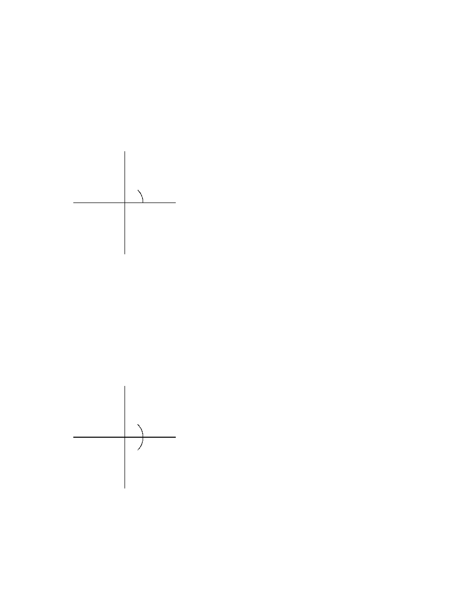
A. & A. Borovik • Mirrors and Reflections • Version 01 • 25.02.00
47
@
@
@
@
@
@
I
6
-
@
@
@
@
@
@
R
?
ψ
The fundamental property of planar
root systems: the angles ψ formed
by pairs of neighbouring roots are
all equal. If the root system con-
tains 2n vectors then ψ = π/n and
the reflection group is the dihedral
group D
2n
of order 2n.
Figure 2.9: A planar root system (Lemma 2.5.1).
@
@
@
@
@
@
@
@
@
@
@
@
α
β
The fact that the angles formed by
pairs of neighbouring roots are all
equal becomes obvious if we con-
sider the corresponding system of
mirrors:
α = β because the ad-
jacent angles are mirror images of
each other.
Figure 2.10: A planar mirror system (for the proof of Lemma 2.5.1).
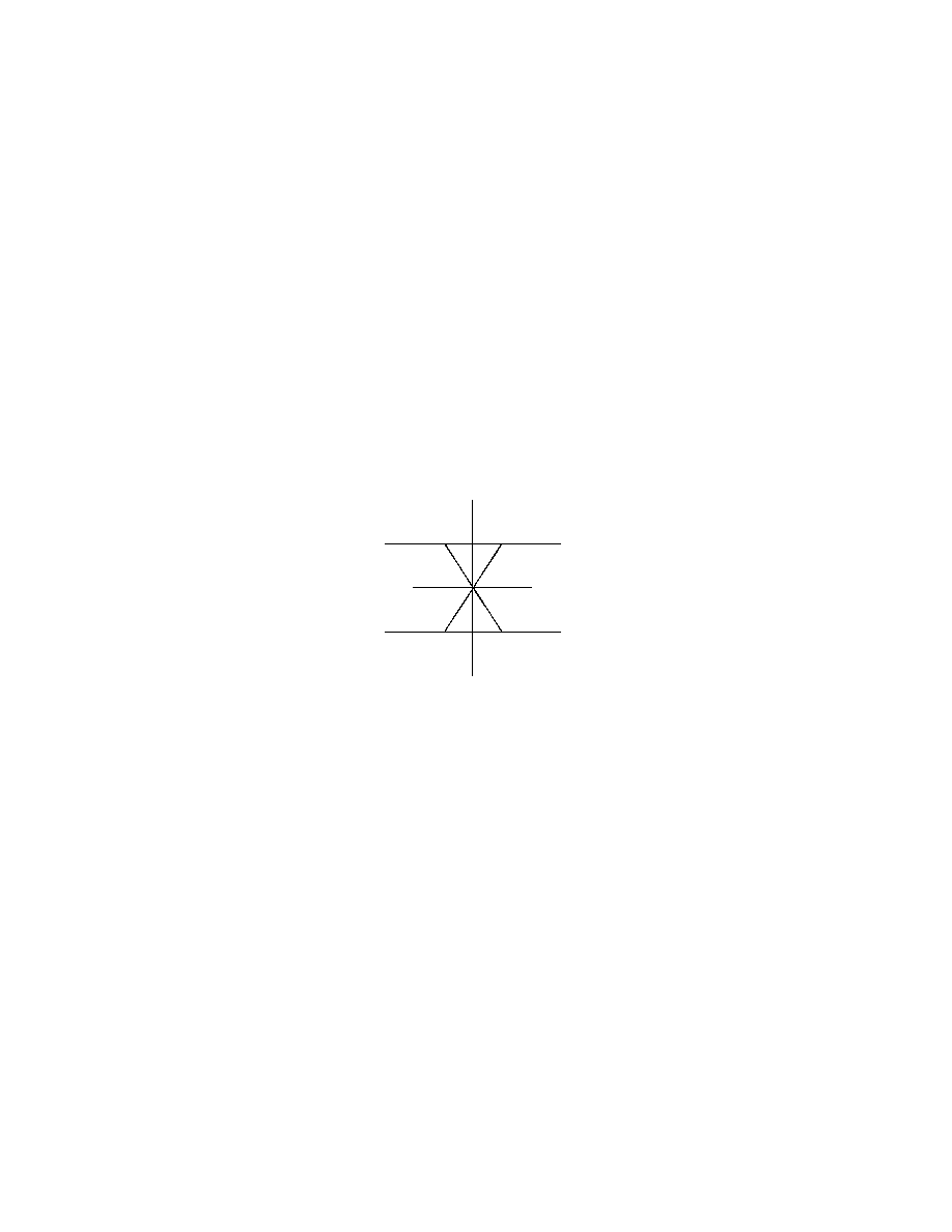
48
Proof
left to the reader as an exercise.
We see that a planar root system consisting of 2n vectors of equal length
is uniquely defined, up to elation of
R
2
. We shall denote it I
2
(n). Later we
shall introduced planar root systems A
2
(which coincides with I
2
(3)) as a
part of series of n-dimensional root systems A
n
. In many applications of
the theory of reflection groups the lengths of roots are of importance; in
particular, the root system I
2
(4) associated with the system of mirrors of
symmetry of the square, comes in two versions, named B
2
and C
2
, which
contain 8 roots of two different lengths, see Figure 2.17 in Section 2.8.
Finally, the regular hexagon gives rise to the root system of type G
2
, see
Figure 2.11.
J
J
J
J
J
J
J
J
J
J
J
J
J
J
J
J
J
J
6
*
H
H
H
H
HH
j
?
H
H
H
H
H
H
Y
-
^
]
Figure 2.11: The root system G
2
Exercises
2.5.1 Prove Lemma 2.5.2.
Hint: Find a regular n-gon such that W (Φ) coincides with its symmetry group.
2.5.2 Prove that, in a root system in
R
2
, the lengths of roots can take at most
two values.
Hint: Use Exercise 2.3.6.
2.5.3 Describe planar root systems with 2 and 4 roots and the corresponding
reflection groups.
2.5.4 Use the observation that the root system G
2
contains two subsystems of
type A
2
to show that the dihedral group D
12
contains two different subgroups
isomorphic to the dihedral group D
6
.

A. & A. Borovik • Mirrors and Reflections • Version 01 • 25.02.00
49
2.5.5 Crystallographic root systems. For the root systems Φ of types
A
2
, B
2
, C
2
, G
2
, sketch the sets Λ =
ZΦ of points in R
2
which are linear combi-
nations of roots in Φ with integer coefficients,
Λ =
(
X
α∈Φ
a
α
α | a
α
∈ Z
)
.
Observe that Λ is a subgroup of
R
2
and, moreover, a discrete subgroup of
R
2
,
that is, there is a real number d > 0 such that, for any λ ∈ Λ, the circle
{ α ∈ R
2
| d(α, λ) < d } contains no points from Λ other than λ. We shall call
root systems in
R
n
with the analogous property crystallographic root systems.
2.6
Positive and simple systems
Positive systems.
Let f :
R
n
−→ R be a linear functional. Assume that
f does not vanish on roots in Φ, i.e. f (α) 6= 0 for all α ∈ Φ. Then every
root ρ in Φ is called positive or negative, according to whether f (ρ) > 0
or f (ρ) < 0. We shall write, abusing notation, α > β if f (α) > f (β).
The system of all positive roots will be denoted Φ
+
and called the positive
system. Correspondingly the negative system is denoted Φ
−
. Obviously
Φ = Φ
+
t Φ
−
.
Let Γ denotes the convex polyhedral cone spanned by the positive sys-
tem Φ
+
. We follow notation of Section 1.5 and call the positive roots s
directed along the edges of Γ simple roots. The set of all simple roots
is called the simple system of roots and denoted Π; roots in Π are called
simple roots. It is intuitively evident that the cone Γ is generated by sim-
ple roots, see also Lemma 1.5.3. In particular, every root φ in Φ
+
can be
written as a non-negative combination of roots in Π:
φ = c
1
ρ
1
+ · · · + c
m
ρ
m
, c
i
> 0, ρ
i
∈ Π.
Notice that the definition of positive, negative, simple systems depends
on the choice of the linear functional f . We shall call a set of roots positive,
negative, simple, if it is so for some functional f .
Lemma 2.6.1 In a simple system Π, the angle between two distinct roots
is non-acute: (α, β)
6 0 for all α 6= β in Π.
Proof.
Let P be a two-dimensional plane spanned by α and β. Denote
Φ
0
= Φ ∩ P . If γ, δ ∈ Φ
0
then the reflection s
γ
maps δ to the vector
s
γ
δ = δ −
2(γ, δ)
(γ, γ)
γ
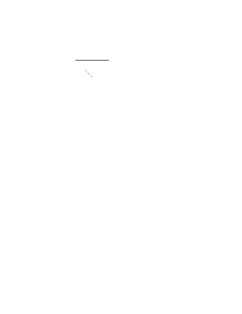
50
A
A
A
U
A
A
A
K
@
@
@
H
H
H
α
β
Plane P
spanned by
α and β
Positive
cone Γ
Planar root system Φ
0
gener-
ated by two simple roots α and
β.
Figure 2.12: For the proof of Lemma 2.6.1
which obviously belongs to P and Φ
0
. Hence every reflection s
γ
for γ ∈ Φ
0
obviously maps P to P and Φ
0
to Φ
0
. This means that Φ
0
is a root system
in P and Φ
+
∩ P is a positive system in Φ
0
.
Moreover, the convex polyhedral cone Γ
0
spanned by Φ
+
0
= Φ
+
∩ P is
contained in Γ ∩ P . Since α and β are obviously directed along the edges
of Γ ∩ P (see also Lemma 1.5.4) and belong to Γ
0
, Γ
0
= Γ ∩ P and α and β
belong to a simple system in Φ
0
, see Figure 2.12. Therefore the lemma is
reduced to the 2-dimensional case, where it is self-evident, see Figure 2.13.
Notice that our proof of Lemma 2.6.1 is a manifestation of a general
principle: surprisingly many considerations in roots systems can be reduced
to computations with pairs of roots.
Theorem 2.6.2 Every simple system Π is linearly independent. In par-
ticular, every root β in Φ can be written, and in a unique way, in the form
P
c
α
α where α ∈ Π and all coefficients c
α
are either non-negative (when
β ∈ Φ
+
) or non-positive (when β ∈ Φ
−
).
Proof.
Assume, by way of contradiction, that Π is linearly dependent
and
X
α∈Π
a
α
α = 0
where some coefficient a
α
6= 0. Rewrite this equality as
P
b
β
β =
P
c
γ
γ
where the coefficients are strictly positive and the sums are taken over
disjoint subsets of Π. Set σ =
P
b
β
β. Since all roots β are positive, σ 6= 0.
But
0
6 (σ, σ) =
X
β
b
β
β,
X
γ
c
γ
γ
!
=
X
β
X
γ
b
β
c
γ
(β, γ)
6 0,
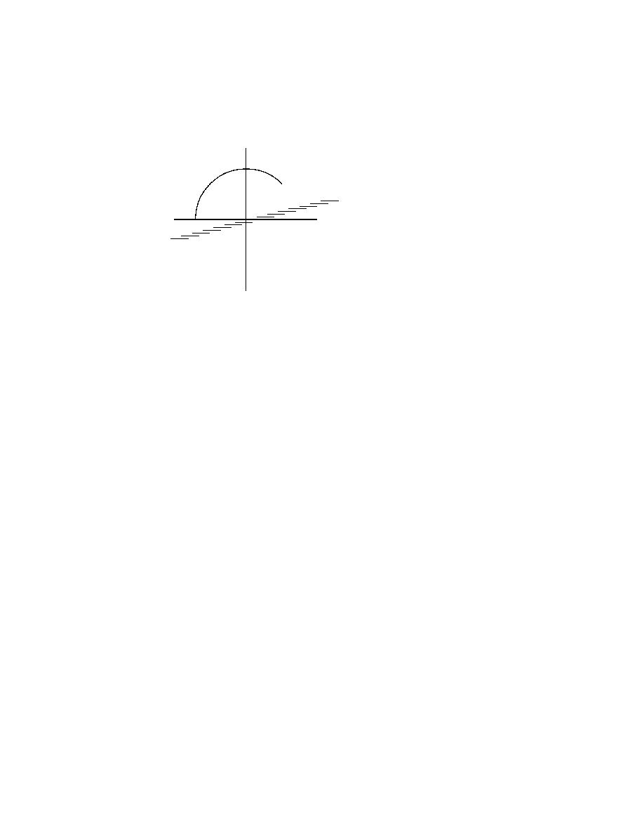
A. & A. Borovik • Mirrors and Reflections • Version 01 • 25.02.00
51
@
@
@
@
@
@
I
6
-
@
@
@
@
@
@
R
?
α
β
Φ
−
Φ
+
positive
halfplane, f (γ) > 0
negative
halfplane, f (γ) < 0
positive
cone Γ
Figure 2.13:
For the proof of Lemma 2.6.1. In the 2-dimensional case the
obtuseness of the simple system is obvious: the roots α and β are directed along
the edges of the convex cone spanned by Φ
+
and the angle between α and β is
at least π/2.
because all individual scalar products (β, γ) are non-positive by Lemma 2.6.1.
Therefore σ = 0, a contradiction.
Corollary 2.6.3 All simple systems in Φ contain an equal number of
roots.
Proof.
Indeed, it follows from Theorem 2.6.2 that a simple system is a
maximal linearly independent subset of Φ.
The number of roots in a simple system of the root system Φ is called
the rank of Φ and denoted rk Φ. The subscript n in the standard notation
for root systems A
n
, B
n
, etc. (which will be introduced later) refers to their
ranks.
Exercises
2.6.1 Prove that, in a planar root system Φ ⊂ R
2
, all positive (correspondingly,
simple) systems are conjugate under the action of the reflection group W =
W (Φ).
2.7
Root system A
n−1
.
Permutation representation of Sym
n
.
Let V be the real vector space
R
n
with the standard orthonormal basis
1
, . . . ,
n
and the corresponding
coordinates x
1
, . . . , x
n
.

52
The group W = Sym
n
acts on V in the natural way, by permuting the
n vectors
1
, . . . ,
n
:
w
i
=
wi
,
which, obviously, induces an action of W on Φ. The action of the group
W = Sym
n
on V =
R
n
preserves the standard scalar product associated
with the orthonormal basis
1
, . . . ,
n
. Therefore W acts on V by orthogonal
transformations.
In its action on V the transposition r = (ij) acts as the reflection in
the mirror of symmetry given by the equation x
i
= x
j
.
Lemma 2.7.1 Every reflection in W is a transposition.
Proof.
The cycle (i
1
· · · i
k
) has exactly one eigenvalue 1 when restricted
to the subspace
R
i
1
⊕ · · · ⊕ R
i
k
, with the eigenvector
i
1
+ · · · +
i
k
. It
follows from this observation that the multiplicity of eigenvalue 1 of the
permutation w ∈ Sym
n
equals the number of cycles in the cycle decom-
position of w (we have to count also the trivial one-element cycles of the
form (i)). If w is a reflection, then the number of cycles is n − 1, hence w
is a transposition.
Regular simplices.
The convex hull ∆ of the points
1
, . . . ,
n
is the
convex polytope defined by the equation and inequalities
x
1
+ · · · + x
n
= 1, x
1
> 0, . . . , x
n
> 0.
Since the group W = Sym
n
permutes the vertices of ∆, it acts as a group
of symmetries of ∆, W
6 Sym ∆. We wish to prove that actually W =
Sym ∆. Indeed, any symmetry s of ∆ acts on the set of vertices as some
permutation w ∈ Sym
n
, hence the symmetry s
−1
w fixes all the vertices
1
, . . . ,
n
of ∆ and therefore is the identity symmetry.
The polytope ∆ is called the regular (n − 1)-simplex. When n = 3, ∆ is
an equilateral triangle lying in the plane x
1
+ x
2
+ x
3
= 1 (see Figure 2.14),
and when n = 4, ∆ is a regular tetrahedron lying in the 3-dimensional
affine Euclidean space x
1
+ x
2
+ x
3
+ x
4
= 1.
The root system A
n−1
.
We shall introduce the root system Φ of type
A
n−1
, as the system of vectors in V =
R
n
of the form
i
−
j
, where
i, j = 1, 2, . . . , n and i 6= j. Notice that Φ is invariant under the action of
W = Sym
n
on V .
In its action on V the transposition r = (ij) acts as the reflection in
the mirror of symmetry perpendicular to the root ρ =
i
−
j
. Hence Φ is
a root system. Since the symmetric group is generated by transpositions,
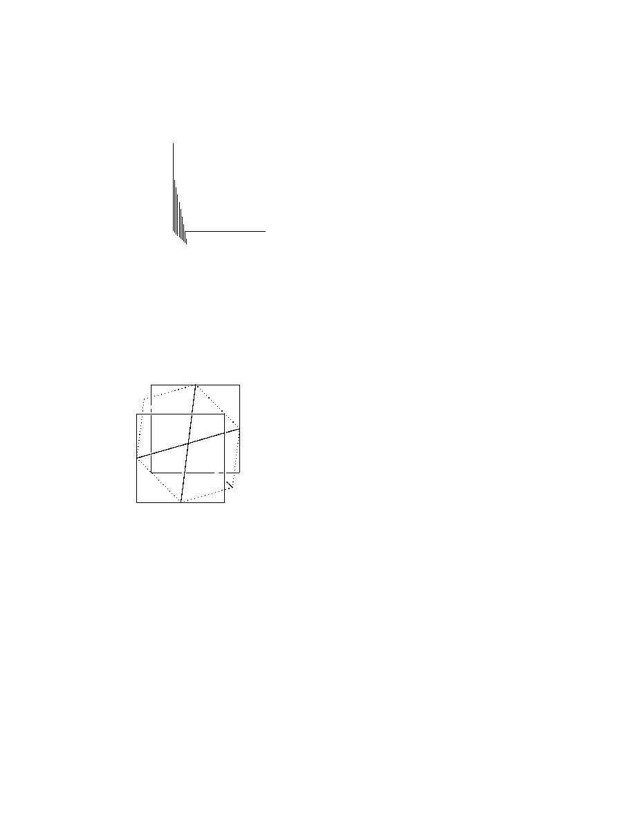
A. & A. Borovik • Mirrors and Reflections • Version 01 • 25.02.00
53
6
-
x
1
x
2
x
3
(1, 0, 0)
(0, 1, 0)
(0, 0, 1)
x
1
= x
2
@
@
D
D
D
D
D
D
DD
@
@
@
@
@
@
The transposition (12) acts on
R
3
as the reflection in the mirror
x
1
= x
2
and as a symmetry of
the equilateral triangle with the
vertices
(1, 0, 0), (0, 1, 0), (0, 0, 1).
Figure 2.14: Sym
n
is the group of symmetries of the regular simplex.
3
−
1
2
−
1
2
−
3
1
−
3
1
−
2
3
−
2
(−1, −1, 1)
(−1, 1, 1)
(1, 1, 1)
(1, −1, 1)
(−1, −1, −1)
(−1, 1, −1)
(1, 1, −1)
(1, −1, −1)
9
@
@
I
@
@
@
:
@
@
@
@
R
The root system {
i
−
j
| i 6= j }
of type A
2
lies in the hyperplane
x
1
+ x
2
+ x
3
= 0 which cuts a regular
hexagon in the unit cube [−1, 1]
3
.
Figure 2.15: Root system of type A
2
.
W = W (Φ) is the corresponding reflection group, and the mirror system
Σ consists of all hyperplanes x
i
= x
j
, i 6= j, i, j = 1, . . . , n.
Notice that the group W is not essential for V ; indeed, it fixes all
points in the 1-dimensional subspace
R(
1
+· · ·+
n
) and leaves invariant the
(n−1)-dimensional linear subpace U defined by the equation x
1
+· · ·+x
n
=
0. It is easy to see that Φ ⊂ U spans U. In particular, the rank of the root
system Φ is n, which justifies the use, in accordance with our convention,
of the index n − 1 in the notation A
n−1
for it.
The standard simple system.
Take the linear functional
f (x) = x
1
+ 2x
2
+ · · · + nx
n
.

54
Obviously f does not vanish on roots, and the corresponding positive sys-
tem has the form
Φ
+
= {
i
−
j
| j < i }.
The set of positive roots
Π = {
2
−
1
,
3
−
2
, . . . ,
n
−
n−1
}
is linearly independent and every positive root is obviously a linear combi-
nation of roots in Π with nonnegative coefficients: for i > j,
i
−
j
= (
i
−
i−1
) + · · · + (
j+1
−
j
),
Therefore Π is a simple system. It is called the standard simple system of
the root system A
n−1
.
Action of Sym
n
on the set of all simple systems.
The following
result is a partial case of Theorem 3.5.1. But the elementary proof given
here is instructive on its own.
Lemma 2.7.2 The group W = Sym
n
acts simply transitively on the set
of all positive (resp. simple) systems in Φ.
Proof.
Since there is a natural one-to-one correspondence between simple
and positive systems, it is enough to prove that W acts simply transitivly
on the set of positive systems in Φ.
Let f be an arbitrary linear functional which does not vanish on Φ,
that is, f (
i
−
j
) 6= 0 for all i 6= j. Then all the values
f (
1
), . . . , f (
n
)
are different and we can list them in the strictly increasing order:
f (
i
1
) < f (
i
2
) < . . . < f (
i
n
).
Now consider the permutation w given, in the column notation, as
w =
1
2
· · · n − 1 n
i
1
i
2
· · ·
i
n−1
i
n
.
Thus the functional f defines a new ordering, wich we shall denote as
6
w
,
on the set [n]:
j
6
w
i if and only if f (
j
)
6 f(
i
).
If we look again at the table for w we see that above any element i in the
bottom row lies, in the upper row, the element w
−1
i. Thus
i
6
w
j if and only if w
−1
i
6 w
−1
j.

A. & A. Borovik • Mirrors and Reflections • Version 01 • 25.02.00
55
Notice also that the permutation w and the associated ordering
6
w
of [n]
uniquely determine each other
6
.
Now consider the positive system Φ
+
0
defined by the functional f ,
Φ
+
0
= {
i
−
j
| f(
i
−
j
) > 0 }.
We have the following chain of equivalences:
i
−
j
∈ Φ
+
0
iff
f (
j
) < f (
i
)
iff
j <
w
i
iff
w
−1
j < w
−1
i
iff
w
−1
i
−
w
−1
j
∈ Φ
+
iff
w
−1
(
i
−
j
) ∈ Φ
+
iff
i
−
j
∈ wΦ
+
.
This proves that Φ
+
0
= wΦ
+
and also that the permutation w is uniquely
determined by the positive system Φ
+
0
. Since Φ
+
, by its construction from
an arbitrary functional, represents an arbitrary positive system in Φ, the
group W acts on the set of positive systems in Φ simply transitively.
Exercises
2.7.1 Make a sketch of the root systems A
1
⊕ A
1
in
R
2
and A
1
⊕ A
1
⊕ A
1
in
R
3
.
2.7.2 Check that, when we take the intersections of the mirrors of reflections
in W = Sym
n
to the subspace x
1
+ · · · + x
n
= 0 of
R
n
, the resulting system of
mirrors can be geometrically described as the system of mirrors of symmetry of
the regular (n − 1)-simplex with the vertices
δ
i
=
i
−
1
n
(
1
+ · · · +
n
), i = 1, . . . , n.
2.7.3 An orthogonal transformation of the Euclidean space
R
n
is called a rota-
tion if its determinant is 1. For a polytope ∆, denote by Rot ∆ the subgroup of
Sym ∆ formed by all rotations. We know that the group of symmetries Sym ∆
of the regular tetrahedron ∆ in
R
3
is isomorphic to Sym
4
; prove that Rot ∆ is
the alternating group Alt
4
.
6
In the nineteenth century the orderings, or rearrangements, of [n] were called per-
mutations, and the permutations in the modern sense, i.e. maps from [n] to [n], were
called substitutions. These are two aspects, ‘passive’ and ‘active’, of the same object.
We shall see later that they correspond to treating a permutation as an element of a
reflection group Sym
n
or an element of the Coxeter complex for Sym
n
.

56
2.8
Root systems of type C
n
and B
n
Hyperoctahedral group.
Let
[n] = {1, 2, . . . , n} and [n]
∗
= {1
∗
, 2
∗
, . . . , n
∗
}.
Define the map ∗ : [n] −→ [n]
∗
by i 7→ i
∗
and the map ∗ : [n]
∗
−→ [n] by
(i
∗
)
∗
= i. Then ∗ is an involutive permutation
7
of the set [n] t [n]
∗
.
Let W be the group of all permutations of the set [n] t [n]
∗
which com-
mute with the involution
∗
, i.e. a permutation w belongs to W if and only
if w(i
∗
) = w(i)
∗
for all i ∈ [n] t [n]
∗
. We shall call permutations with this
property admissible. The group W is known under the name of hyperoc-
tahedral group BC
n
. It is easy to see that W is isomorphic to the group
of symmetries of the n-cube [−1, 1]
n
in the n-dimensional real Euclidean
space
R
n
. Indeed, if
1
,
2
, . . . ,
n
is the standard orthonormal basis in
R
n
,
we set, for i ∈ [n],
i
∗
= −
i
. Then we can define the action of W on
R
n
by the following rule: w
i
=
wi
. Since w is an admissible permutation of
[n] t [n]
∗
, the linear transformation is well-defined and orthogonal. Also it
can be easily seen that W is exactly the group of all orthogonal transfor-
mations of
R
n
preserving the set of vectors {±
1
, ±
2
, . . . , ±
n
} and thus
preserving the cube [−1, 1]
n
. Indeed, the vectors ±
i
, i ∈ [n], are exactly
the unit vectors normal to the (n − 1)-dimensional faces of the cube (given,
obviously, by the linear equations x
i
= ±1, i = 1, 2, . . . , n).
The name ‘hyperoctahedral’ for the group W is justified by the fact
that the group of symmetries of the n-cube coincides with the group of
symmetries of its dual polytope, whose vertices are the centers of the faces
of the cube. The dual polytope for the n-cube is known under the name
of n-cross polytope or n-dimensional hyperoctahedron (see Figure 2.16).
Admissible orderings.
We shall order the set [n] t [n]
∗
in the following
way:
n
∗
< n − 1
∗
< ... < 2
∗
< 1
∗
< 1 < 2 < ... < n − 1 < n.
If now w ∈ W then we define a new ordering 6
w
of the set [n] t [n]
∗
by
the rule
i
6
w
j if and only if w
−1
i
6 w
−1
j.
Orderings of the form
6
w
, w ∈ W , are called admissible orderings of the
set [n] t [n]
∗
. They can be characterized by the following property:
an ordering ≺ on [n] t [n]
∗
is admissible if and only if from
i ≺ j it follows that j
∗
≺ i
∗
.
7
That is, a permutation of order 2.
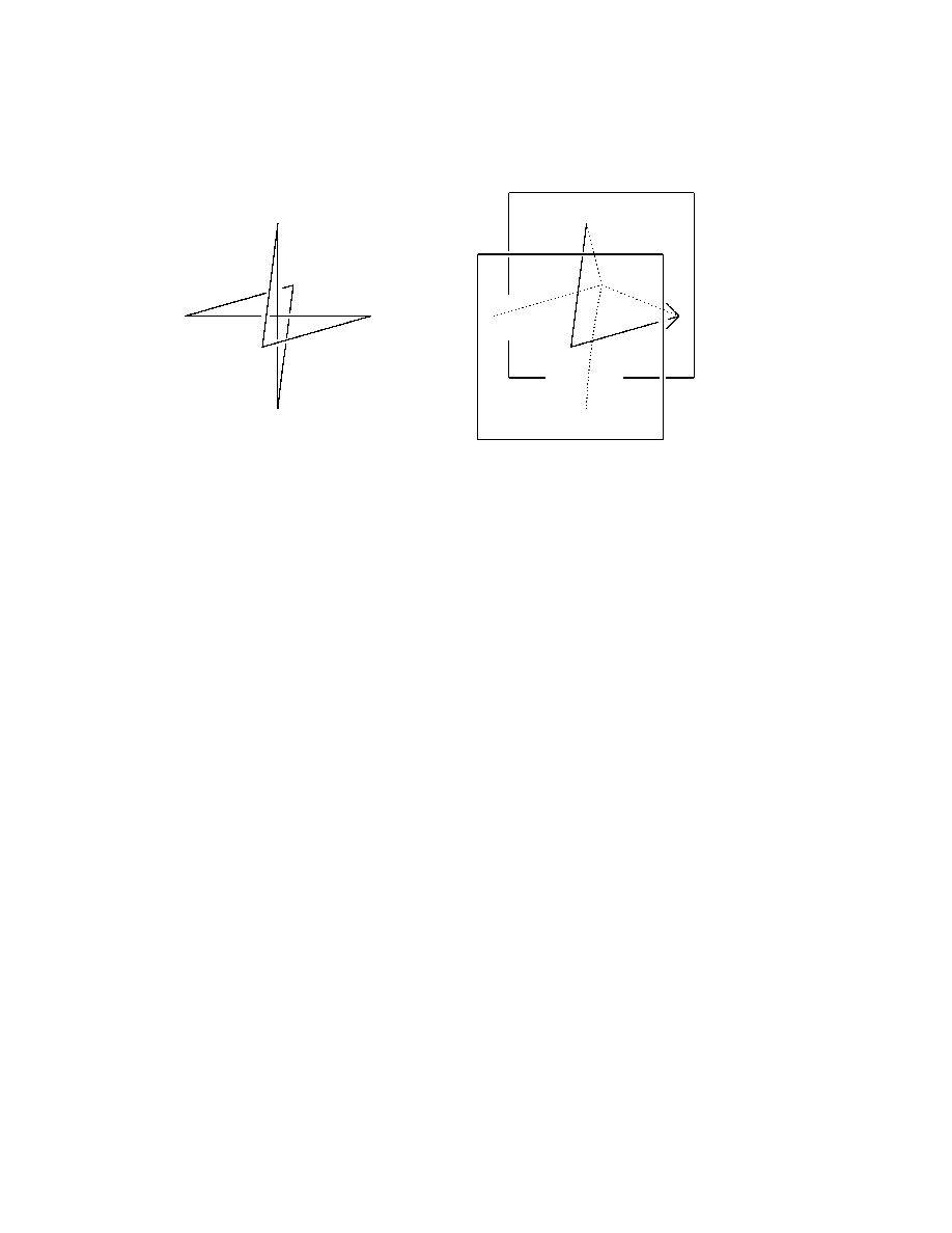
A. & A. Borovik • Mirrors and Reflections • Version 01 • 25.02.00
57
(a)
(b)
−
2
2
−
3
3
−
1
1
@
@
@
@
@
@
@
@
@
@
@
@
a
a
a
a
a
C
C
C
C
-
6
?
@
@
@
@
@
@
@
@
@
@
@
@
a
a
a
a
a
C
C
C
C
aa
aa
a
C
C
C
C
Figure 2.16:
Hyperoctahedron (‘octahedron’ in dimension n = 3) or n-cross
polytope is the convex hull of the points ±
i
, i = 1, . . . , n in
R
n
(picture (a)).
Obviously the hyperoctahedron is the dual polytope to the unit cube (picture
(b)).
Vice versa, if ≺ is an admissible ordering, then the permutation
w =
n
∗
(n − 1)
∗
. . . 1
∗
1
. . . n − 1
n
j
1
j
2
. . . j
n
j
n+1
. . .
j
2n−1
j
2n
where
j
1
≺ j
2
≺ . . . ≺ j
2n−1
≺ j
2n
,
is admissible and the ordering ≺ coincides with 6
w
.
Root systems C
n
and B
n
.
Let
i
, i ∈ [n], be the standard orthonormal
basis in
R
n
, and set
i
∗
= −
i
for i
∗
∈ [n]
∗
. This defines the vectors
j
for all j ∈ [n] t [n]
∗
. Now the root system Φ of type C
n
is formed by
the vectors 2
j
, j ∈ [n] t [n]
∗
(called long roots), together with the vectors
j
1
−
j
2
, where j
1
, j
2
∈ [n] t [n]
∗
, j
1
6= j
2
or j
∗
2
(called short roots). Written
in the standard basis
1
,
2
, . . . ,
n
, the roots take the form ±2
i
or ±
i
±
j
,
i, j = 1, 2, . . . , n, i 6= j. Notice that both short and long roots can be
written as
j
−
i
for some i, j ∈ [n] t [n]
∗
.
It is easy to see that when ρ is one of the long roots ±2
i
, i ∈ [n], then
s
ρ
is the linear transformation corresponding to the element (i, i
∗
) of W
in its canonical representation. Analogously, if ρ =
i
−
j
, is a short root
(recall that we use the convention
i
∗
= −
i
for i ∈ [n]), then the reflection
s
r
corresponds to the admissible permutation (i, j)(i
∗
, j
∗
). Moreover, one
can easily check (for example, by computing the eigenvalues of admissible
permutations from W in their action on
R
n
) that every reflection in the
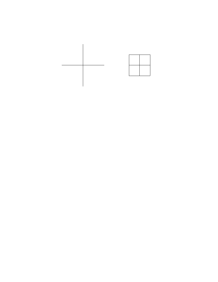
58
C
2
@
@
@
@
@
@
@
@
@
@
@
@
-
6
?
@
@
@
R
@
@
@
I
B
2
@
@
@
@
@
@
@
@
@
@
@
@
-
6
?
@
@
@
R
@
@
@
I
Figure 2.17: Root systems B
2
and C
2
.
group of the symmetries of the unit cube [−1, 1]
n
is of one of these two
types.
Now we see that use of the name ‘root system’ in regard to the set Φ
is justified.
The root system
B
n
= { ±
i
±
j
, ±
i
| i, j = 1, 2 . . . , n, i 6= j }
differs from C
n
only in lengths of roots (see Figure 2.17) and has the same
reflection group BC
n
. Therefore in the sequel we shall deal only with the
root system C
n
.
Action of W on Φ.
Now consider the linear functional
f (x) = x
1
+ 2x
2
+ 3x
3
+ · · · + nx
n
.
It is easy to see that a root
i
−
j
is positive with respect to f if, in the
ordering
n
∗
< n − 1
∗
< . . . < 1
∗
< 1 < 2 < . . . < n
of the set [n] t [n]
∗
, we have i > j. The system of positive roots Φ
+
associated with f is called the standard positive system of roots. The set
Π = {2
1
,
2
−
1
, . . . ,
n
−
n−1
}
is obviously the simple system of roots contained in Φ
+
.
If now
j
1
<
w
j
2
<
w
. . . <
w
j
2n−1
<
w
j
2n
,
is an admissible ordering of [n] t [n]
∗
, then the vectors
j
n+1
,
j
n+2
, . . . ,
j
2n
form a basis in
R
n
. Let y
1
, y
2
, . . . , y
n
be the coordinates with respect to
this basis and f (y) = y
1
+ 2y
2
+ 3y
3
+ · · ·+ny
n
. Then, obviously, f does not
vanish on roots in Φ, and, for a root
j
−
i
in Φ, the inequality f (
j
−
i
) > 0

A. & A. Borovik • Mirrors and Reflections • Version 01 • 25.02.00
59
is equivalent to i
6
w
j. Thus the system of positive roots associated with
f coincides with the system
wΦ
+
= {
j
−
i
| i 6
w
j}
obtained from the standard system Φ
+
of positive roots by the action of
the element w. Obviously, the simple system of roots contained in Φ
+
is
exactly wΠ.
If now Π
0
is an arbitrary simple system of roots arising from an arbitrary
linear function f :
R
n
−→ R not vanishing on roots in Φ then the following
objects are uniquely determined by our choice of Π
0
:
• the system of positive roots Φ
+0
, which can be defined in two equiv-
alent ways: as the set of all roots which are non-negative linear com-
binations of roots from Π
0
, and as the set {r ∈ Φ | f(r) > 0};
• the (obviously admissible) ordering ≺ on J defined by the rule: i ≺ j
if and only if f (
i
)
6 f(
j
).
In particular, we immediately have the following observation (which is a
partial case of a more general result about conjugacy of simple system of
roots for arbitrary finite reflection groups, Theorem 3.5.5).
Proposition 2.8.1 Any two simple systems in the root system Φ of type
B
n
or C
n
are conjugate under the action of W . Moreover, the reflection
group W is simply transitive in its action on the set of simple systems in
Φ.
Exercises.
2.8.1 Prove that every reflection in BC
n
has the form (ii
∗
) or (ij)(i
∗
j
∗
).
2.8.2 Prove that the reflection group of type BC
2
is isomorphic to the dihedral
group D
8
.
2.8.3 The group of symmetries of the cube. Observe that the group
W = BC
3
of symmetries of the cube ∆ = [−1, 1]
3
contains the involution z
which sends every vertex of the cube to its opposite.
1. Check that det z = −1, so that z to the group R = Rot ∆ of rotations of
the cube.
2. Prove that z ∈ Z(W ).
3. Prove that the group R acts faithfully on the set D of 4 diagonals of
the cube ∆, that is, the segments connecting the opposite vertices of the
cube. Moreover, every permutation of diagonals is the result of action of
a rotation of the cube. Hence R ' Sym
4
.

60
4. Prove that W = hzi × R.
5. Prove that hzi = Z(W ).
6. Prove that the symmetries of the cube which send every 2-dimensional
face of the cube into itself or the opposite face form a normal abelian
subgroup E < W of order 8. Prove further that W/E ' Sym
3
and that
actually W = E
o T for some subgroup T ' Sym
3
.
2.8.4 Important root subsystems.
Prove that
1. the set Θ of roots { ±
i
| i = 1, . . . , n } is a root system of type A
1
+· · ·+A
1
(n summands);
2. the intersection Ψ of Φ with the hyperplane x
1
+ · · · + x
n
= 0 is a root
system of type A
n−1
.
2.8.5 The structure of the hyperoctahedral group. Use Exercise 2.8.4
to show that if E and T are the reflection groups corresponding to the systems
of roots Θ and Ψ then
1. E ' Z
2
× · · · × Z
2
(n factors);
2. E
C W ;
3. T ' Sym
n
;
4. W = E
o T .
2.8.6 (R. Sandling) Prove that
Sym [−1, 1]
n
= {w ∈ GL
n
(
R
n
) | w([−1, 1]
n
) = [−1, 1]
n
},
i.e. linear transformations preserving the cube are in fact orthogonal.
2.9
The root system D
n
By definition,
D
n
= { ±
i
±
j
| i, j = 1, 2, . . . , n, i 6= j };
thus D
n
is a subsystem of the root system C
n
.
The system
Π = {
1
+
2
,
2
−
1
,
3
−
2
, . . . ,
n
−
n−1
}
is a simple system in Φ.
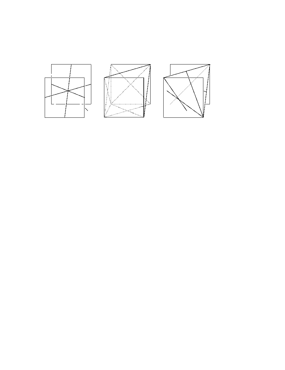
A. & A. Borovik • Mirrors and Reflections • Version 01 • 25.02.00
61
9
y
@
@
I
@
@
@
C
C
CO
:
z
@
@
@
@
R
C
C
CW
@
@
@
@
@
@
@
@
@
aa
aa
aa
a
a
C
C
C
C
C
C
C
C
C
C
C
C
@
@
@
@
@
@
@
@
@
PP
PP
PP
PPP
a
a
a
a
a
a
a
a
Figure 2.18:
Shown are the root system D
3
inscribed into the unit cube [−1, 1]
3
(on the left), and the corresponding mirror system (shown in the middle by
intersections with the surface of the cube and the tetrahedron inscribed in the
cube). Comparing the last two pictures we see that the mirror system of type
D
3
is isometric to the mirror system of type A
3
.
Exercises
2.9.1 Describe explicitly an isometry between the root systems
D
3
= { ±
i
±
j
| i, j = 1, 2, 3, i 6= j }
and
A
3
= {
i
−
j
| i, j = 1, 2, 3, 4, i 6= j }
(see Figure 2.18).
2.9.2 Sketch the root system D
2
; you will see that it consists of two orthogonal
pairs of vectors, each forming the 1-dimensional system A
1
. Thus D
2
= A
1
+ A
1
.

62

Chapter 3
Coxeter Complex
3.1
Chambers
Chambers.
Consider the system Σ of all mirrors of reflections s
ρ
for
ρ ∈ Φ. Of course, this a hyperplane arrangement in the sense of Section 1.2,
and we shall freely use the relevant terminology. In particular, chambers
of Σ are open polyhedral cones—connected components of V
r
S
H∈Σ
H.
The closures of these cones are called closed chambers. Facets of chambers
(i.e. faces of maximal dimension) are panels and mirrors in Σ as walls.
Notice that every panel belongs to a unique wall. To fully appreciate this
architectural terminology (introduced by J. Tits), imagine a building built
out of walls of double-sided mirrors. Two chambers are adjacent if they
have a panel in common. Notice that every chamber is adjacent to itself.
Theorem 3.1.1 Every chamber C has the form
T
ρ∈Π
V
−
ρ
for some simple
system Π. Every panel of C belongs to one of the walls H
ρ
for a root ρ ∈ Π.
Vice versa, if ρ ∈ Π then H
ρ
∩ C is a panel of C.
Proof.
Take any vector γ in the chamber C and consider the linear func-
tional f (λ) = −(γ, λ). Since γ does not belong to any mirror H
α
in Σ,
the functional f does not vanish on roots in Φ. Therefore the condition
f (α) > 0 determines a positive system Φ
+
and the corresponding simple
system Π. Now consider the cone C
0
defined by the inequalities (λ, ρ) < 0
for all ρ ∈ Π. Obviously γ ∈ C
0
and therefore C ⊆ C
0
. If C 6= C
0
then some hyperplane H
α
, α ∈ Φ, bounds C and intersects C
0
nontriv-
ially. But α =
P
c
ρ
ρ where all c
ρ
are all non-negative or all non-positive,
and (γ, α) =
P
c
ρ
(γ, ρ) cannot be equal 0. This contradiction shows that
C = C
0
. The closure C of C is defined by the inequalities (λ, ρ)
6 0 for
ρ ∈ Π which is equivalent to (λ, α) 6 0 for α ∈ Γ. Therefore the cone
63
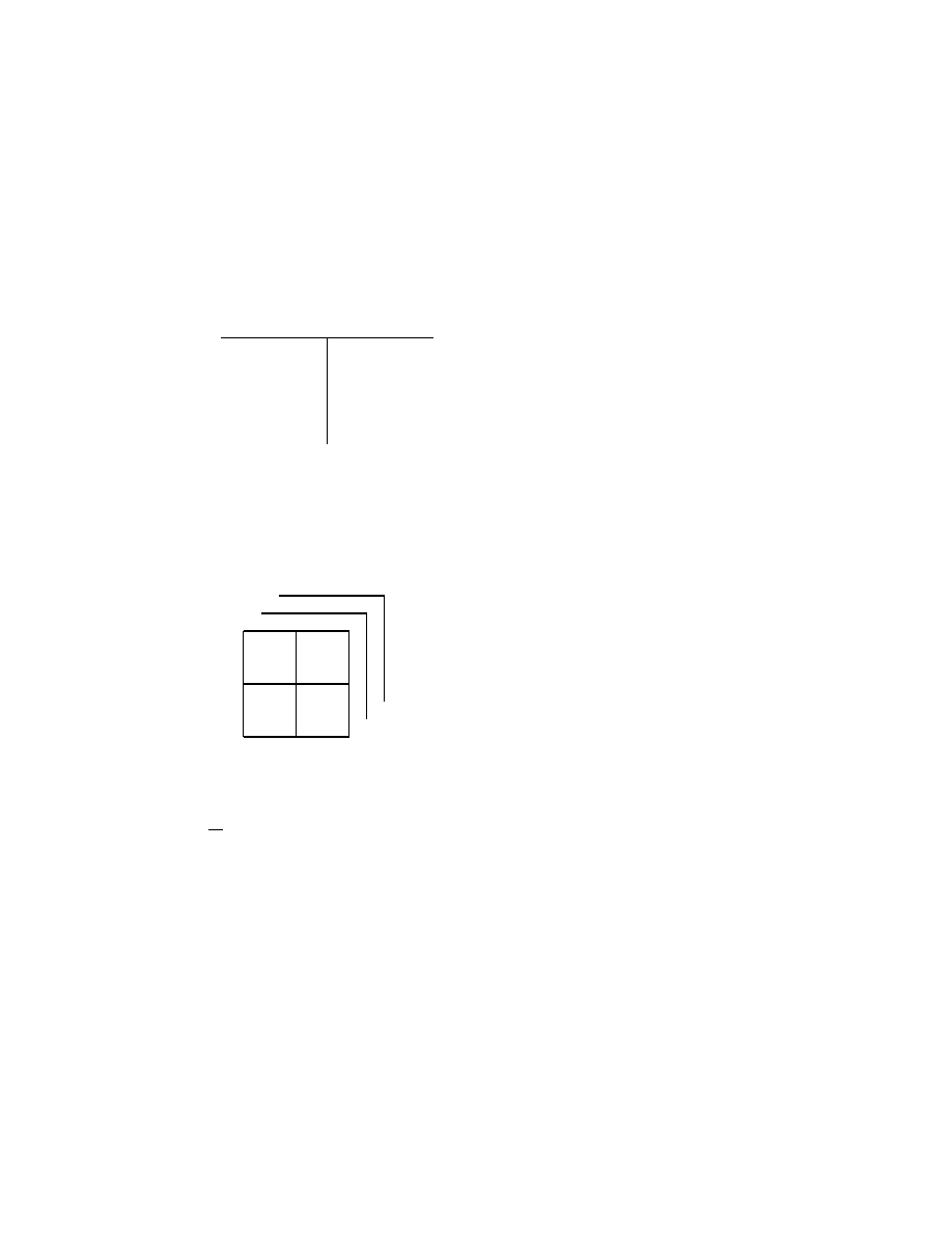
64
A
A
A
A
A
A
K
-
A
A
A
A
AAU
Q
Q
Q
Q
Q
Q
A
A A
A A
A A
A A
A A
A A
A A
A
A
A
A
A
A
A
A
A
A
A
A
A
A
A
A
A
Positive cone Γ
Fundamental
chamber C
The fundamental chamber C is
defined as the interior of the cone
dual to the positive cone Γ, i.e.
as the set of vectors λ such that
(λ, γ) < 0 for all γ ∈ Γ.
Figure 3.1: The fundamental chamber.
H
H
H
H
H
A
A
A
A
A
@
@
@
@
@
@
@
The Coxeter complex of type BC
3
is
formed by all the mirrors of symmetry of
the cube; here they are shown by their
lines of intersection with the faces of the
cube.
Figure 3.2: The Coxeter complex BC
3
.
C is dual to the positive cone Γ (see Figure 3.1) and every facet of C is
perpendicular to some edge of Γ, and vice versa. In particular, every panel
of C belongs to the wall H
ρ
for some simple root ρ ∈ Π.
The same argument works in the reverse direction: if Π is any simple
system then, since Π is linearly independent, we can find a vector γ such
that (γ, ρ) < 0 for all ρ ∈ Π. Then (γ, α) 6= 0 for all roots α ∈ Φ and the
chamber C containing γ has the form C =
T
ρ∈Π
V
−
ρ
.
The set of all chambers associated with the root system Φ is called the
Coxeter complex and will be denoted by C. See, for example, Figures 3.2
and 3.3. If Π is a simple system then the corresponding chamber is called
the fundamental chamber of C.
The following lemma is an immediate consequence of Lemma 1.2.3
Lemma 3.1.2 The union of two distinct adjacent closed chambers is con-
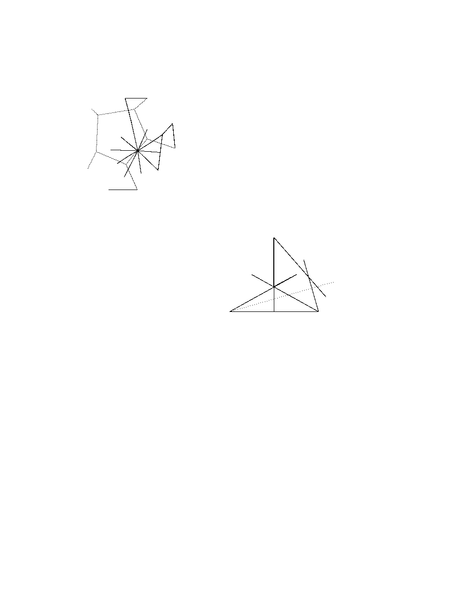
A. & A. Borovik • Mirrors and Reflections • Version 01 • 25.02.00
65
E
E
EE
XXXX
@
@
@
@
@
@
@,
,
,
!!
!!
\
\
%
%
%
%
A
A
A
A
PP
PP
P
In the case that Σ is the system
of mirrors of symmetry of a regu-
lar polytope ∆, the Coxeter complex
is basically the c subdivision of the
faces of ∆ by the mirrors of sym-
metries of faces (here shown only on
one face of the dodecahedron ∆).
Figure 3.3:
Chambers and baricentric subdivision
T
T
T
T
T
Z
Z
Z
Z
Z
Z
Z
Z
T
T
T
T
T
T
T
T
T
T
````
`
(23)
(34)
(12)
1
2
3
4
The symmetry group of the tetra-
hedron acts on its 4 vertices as
the symmetric group Sym
4
. The
reflections in the walls of the fun-
damental chamber are the trans-
positions (12), (23) and (34).
Therefore they generate Sym
4
.
Figure 3.4: Generation by simple reflections (Theorem 3.2.1).
vex.
3.2
Generation by simple reflections
Simple reflections.
Let Π = { ρ
1
, . . . , ρ
n
} be a simple system of roots.
The corresponding reflections r
i
= s
ρ
i
are called simple reflections.
Theorem 3.2.1 The group W is generated by simple reflections.
Proof.
Set W
0
= hr
1
, . . . , r
n
i. We shall prove first that
the group W
0
is transitive in its action on C.
Proof of the claim. The fundamental chamber C is bounded by panels lying
on the mirrors of the simple reflections r
1
, . . . , r
n
. Therefore the neighbour-
ing chambers (i.e. the chambers sharing a common mirror with C) can be
obtained from C by reflections in these mirrors and equal r
1
C, . . . , r
n
C.

66
Let now w ∈ W
0
, then the panels of the chamber wC belong to the mirrors
of reflections wr
1
w
−1
, . . . , wr
n
w
−1
. If D is a chamber adjacent to wC then
it can be obtained from wC by reflecting wC in the common mirror, hence
D = wr
i
w
−1
·wC = wr
i
C for some i = 1, . . . , n. Notice that wr
i
∈ W
0
. We
can proceed to move from a chamber to an adjacent one until we present
all chambers in C in the form wC for appropriate elements w ∈ W .
We can now complete the proof. If α ∈ Φ is any root and s
α
the
corresponding reflection then the wall H
α
bounds some chamber D. We
know that D = wC for some w ∈ W
0
. The fundamental chamber C is
bounded by the walls H
ρ
i
for simple roots ρ
i
(Theorem 3.1.1) and therefore
the wall H
α
equals wH
ρ
i
for some simple root ρ
i
. Thus s
α
= wr
i
w
−1
belongs
to W
0
. Since the group W is generated by reflections s
α
we have W = W
0
.
In the course of the proof we have obtained one more important result:
Corollary 3.2.2 The action of W on C is transitive.
This observation will be later incorporated into Theorem 3.5.1.
Exercises
3.2.1 Use Theorem 3.2.1 to prove the (well-known) fact that the symmetric
group Sym
n
is generated by transpositions (12), (23), . . . , (n − 1, n) (see Fig-
ure 3.4).
3.2.2 Prove that the reflections
r
1
= (12)(1
∗
2
∗
), . . . , r
n−1
= (n − 1, n)(n − 1
∗
, n
∗
), r
n
= (n, n
∗
)
generate the hyperoctahedral group BC
n
.
3.3
Foldings
Given a non-zero vector α ∈ V , the hyperplane H
α
= { γ ∈ V | (γ, α) = 0 }
cuts V in two subspaces
V
+
α
= { γ | (γ, α) > 0 } and V
−
α
= { γ | (γ, α) 6 0 }
intersecting along the common hyperplane H
α
. The folding in the direction
of α is the map f
α
defined by the formula
f
α
(β) =
β
if (β, α)
> 0
s
α
β
if (β, α) < 0
.
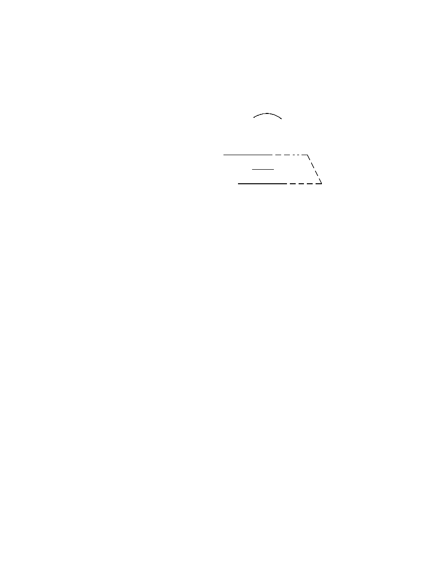
A. & A. Borovik • Mirrors and Reflections • Version 01 • 25.02.00
67
R
2
V
+
α
H
α
V
−
α
α
f
α
+
A
A
A
A
A
A
A
A
A
A
A
A
In the 2-dimensional case, a
folding is exactly what its
name suggests: the plane is
being folded on itself like a
sheet of paper.
Figure 3.5: Folding
Thus f
α
fixes all points in V
+
α
and maps V
−
α
onto V
+
α
symmetrically (see
Figure 3.5). Notice that f
α
is an idempotent map, i.e. f
α
f
α
= f
α
. The
folding f
−α
is called the opposite to f
α
. The reflection s
α
is made up of
two foldings f
α
and f
−α
:
s
α
= f
α
|
V
+
α
∪ f
−α
|
V
−
α
.
We say that a folding f covers a subset X ⊂ V if X ⊆ f(V ).
By definition, a folding of the chamber complex C is a folding along one
of its walls.
Proposition 3.3.1 A folding f of C sends chambers to chambers and pre-
serves adjacency: if C and D are two adjacent chambers then their images
f (C) and f (D) are also adjacent. (Remember that, by definition of adja-
cency, this includes the possibility that f (C) = f (D).)
Exercises
3.3.1 When you fold a sheet of paper, why is the line along which it is folded
straight?
3.3.2 There are three foldings of the chamber complex BC
2
such that their
composition maps the chamber complex onto one of its chambers. What is the
minimal number of foldings needed for folding the chamber complex BC
3
onto
one chamber?
3.4
Galleries and paths
Galleries.
Given two chambers C and D, we can always find a sequence
G of chambers C = C
0
, C
1
, . . . , C
l−1
, C
l
such that every two consequtive

68
chambers C
i−1
and C
i
are adjacent. We shall call G a gallery connecting
the chambers C and D. Notice that our definition of adjacency allows that
two adjacent chambers coincide. This means that we also allow repetition
of chambers in a gallery: it could happen that C
i−1
= C
i
. We shall say in
this situation that the gallery stutters at chamber C
i
. The number l will
be called the length of the gallery G.
Notice that if s
i
is the reflection in a common wall of two adjacent
chambers C
i−1
and C
i
then either C
i
= s
i
C
i−1
or C
i
= C
i−1
.
Given w ∈ W , we wish to describe a canonical way of connecting the
fundamental chamber C and the chamber D = wC by a gallery.
We
know that W is generated by the fundamental reflections r
1
, . . . , r
n
, i.e.
the reflections in the walls of the fundamental chamber C. The minimal
number l such that w is the product of some l fundamental reflections is
called the length of w and denoted as l(w).
Let w = r
i
1
· · · r
i
l
. We leave to the reader to check the following group
theoretical identity: since all r
i
are involutions,
r
i
1
· · · r
i
l
= r
r
il−1
···r
i1
i
l
· r
r
il−2
···r
i1
i
l−1
· · · r
r
i1
i
2
· r
i
1
.
Denote s
j
= r
r
j−1
···r
i1
i
j
, then w = s
l
· · · s
1
and, moreover,
s
j
· · · s
1
= r
i
1
· · · r
i
j
for j = 1, . . . , l.
Define by induction C
0
= C and, for i = 1, . . . , l, C
j
= s
j
C
i−1
, so that
C
j
= s
j
· · · s
1
C
0
= r
i
1
· · · r
i
j
C
0
for j > 0,
C
l
= r
i
1
· · · r
i
l
C
0
= wC = D.
Notice that s
1
= r
1
is the reflection in the common wall of the chambers
C
0
and C
1
. Next, s
j
for j > 1 is written as
s
j
= r
r
ij−1
···r
i1
i
j
= (r
i
1
· · · r
i
j−1
)r
i
j
(r
i
1
· · · r
i
j−1
)
−1
.
By Lemma 2.1.3, since r
i
j
is a reflection in a panel, say H, of the funda-
mental chamber C = C
0
, s
j
is the reflection in the panel r
i
1
· · · r
i
j−1
H of
the chamber r
i
1
· · · r
i
j−1
C
0
= C
j−1
. Since s
j
C
j−1
= C
j
,
s
j
is the reflection in the common panel of the chambers C
j−1
and C
j
.
Summarising this procedure we obtain the following result; it will show
us the right way in the labyrinth of mirrors.

A. & A. Borovik • Mirrors and Reflections • Version 01 • 25.02.00
69
Theorem 3.4.1 Let w = r
i
1
· · · r
i
l
be an expression of w ∈ W in terms of
simple reflections r
i
. Let C be the fundamental chamber and D a chambers
in C such that D = wC. Then there exists a unique gallery C
0
, C
1
, . . . , C
l
connecting C = C
0
and D = C
l
with the following property:
s
j
= r
r
j−1
···r
i1
i
j
is the reflection in the common wall of C
j−1
and
C
j
, j = 1, . . . , l and w = s
l
· · · s
1
.
The gallery C
0
, . . . , C
l
constructed in Theorem 3.4.1 will be called the
canonical w-gallery starting at C = C
0
.
We can reverse the above arguments and obtain also the following re-
sult.
Theorem 3.4.2 Let C
0
, . . . , C
l
be a gallery connecting the fundamental
chamber C = C
0
and a chamber D = C
l
. Assume that the gallery does
not stutter at any chamber, that is, no two consequent chambers C
i
and
C
i+1
coincide. Let s
i
be the reflection in the common wall of C
i−1
and C
i
,
i = 1, . . . , l
Then D = wC for w = s
l
· · · s
1
,
C
j
= s
j
· · · s
1
C
0
for all j = 1, . . . , l,
and there exists an expression w = r
i
1
· · · r
i
l
of w in terms of simple reflec-
tions r
i
such that, for all j = 1, . . . , l,
s
j
= r
r
j−1
···r
i1
i
j
.
3.5
Action of W on C
In this section we shall prove arguably the most important property of the
Coxeter complex.
Theorem 3.5.1 The group W is simply transitive on C, i.e. for any two
chambers C and D in C there exists a unique element w ∈ W such that
D = wC.
Paths.
We shall call a sequence of points γ
0
, . . . , γ
l
a path if
• the consecutive points γ
i−1
and γ
i
are contained in adjacent chambers
C
i−1
and C
i
;

70
• if C
i−1
= C
i
then γ
i−1
= γ
i
;
• if C
i−1
6= C
i
and s
i
is the reflection in the common panel of C
i−1
and
C
i
then γ
i
= s
i
γ
i−1
.
The number l is called the length of the path. Set w = s
l
· · · s
0
. Since
γ
l
= s
l
· · · s
1
γ
0
= wγ
0
,
the sequence of chambers C
0
, C
1
, . . . , C
l
is the canonical w-gallery, and, by
Theorem 3.4.2, w can be expressed as a product of l simple reflections. So
we have the following useful lemma.
Lemma 3.5.2 Given a path γ
0
, γ
1
, . . . , γ
l
, there exists w ∈ W such that
γ
l
= wγ
0
and l(w)
6 l.
Notice the important property of paths: since we know that the union
of two distinct adjacent closed chambers is convex (Lemma 3.1.2), the
wall H
s
i
is the only wall intersecting the segment [γ
i−1
γ
i
]. Therefore the
following lemma holds.
Lemma 3.5.3 If γ
0
, . . . , γ
l
is a path connecting the points γ
0
and γ
l
lying
on the opposite sides of the wall H. Then the path intersects H in the sense
that, for some two consecutive points γ
i−1
and γ
i
, the wall H intersects
the segment [γ
i−1
, γ
i
] and
• the common panel of the chambers C
i−1
and C
i
containing γ
i−1
and
γ
i
, respectively, belongs to H;
• γ
i−1
and γ
i
are symmetric in H.
Paths and foldings.
As often happens in the theory of reflection groups,
an important technical result we wish to state now can be best justified by
referring to a picture (Figure 3.6).
Lemma 3.5.4 Assume that the starting point α = γ
0
and the end point
ω = γ
l
of a path γ
0
, . . . , γ
l
lie on one side of a wall H. If the wall H
intersects the path, that is, one of the points γ
i
lies on the opposite side of
H from α, then the path can be replaced by a shorter path with the same
starting and end points, and such that it does not intersect the wall H.
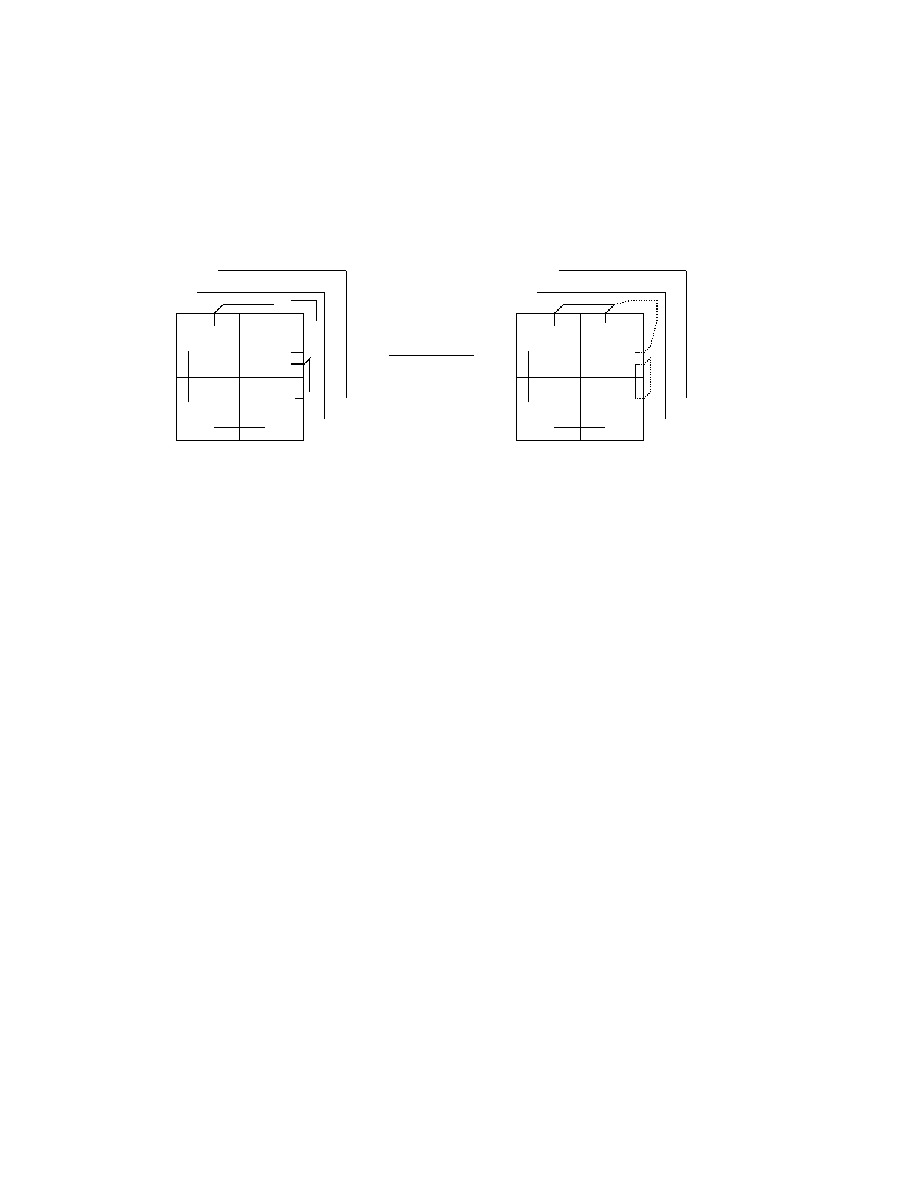
A. & A. Borovik • Mirrors and Reflections • Version 01 • 25.02.00
71
H
H
H
H
HH
H
H
H
H
HH
-
ω
α
r
9
?
?
@
@
R
-
6
?
?
@
@
R
-
6
ω
α
r
@
@
I
H
H
H
H
H
H
H
H
A
A
A
A
A
A
@
@
@
@
@
@
@
@
@
H
H
H
H
H
H
A
A
A
A
A
A
@
@
@
@
@
@
@
@
@
Figure 3.6:
For the proof of Lemma 3.5.4: the folding in a wall which intersects
a path converts the path to a shorter one.
Proof.
See the quite self-explanatory Figure 3.6. A rigorous proof fol-
lows. However, it can be skipped in the first reading.
Assume that the path intersects the wall H at the segment
[γ
p
1
−1
γ
p
1
]. Then, in view of Lemma 3.5.3, the path should intersect
the wall at least once more, say at the segments
[γ
p
2
−1
γ
p
2
], . . . , [γ
p
k
−1
γ
p
k
].
Let C
0
, . . . , C
l
be the gallery corresponding to our path, so that
γ
i
∈ C
i
. Take the folding f in H onto the half space containing α
and β and consider the path f (γ
0
), f (γ
1
), . . . , f (γ
l
) and the gallery
f (C
0
), f (C
1
), . . . , f (C
l
). In this new gallery and new path we have
repeated chambers, namely.
f (C
p
1
−1
) = f (C
p
1
), . . . , f (C
p
k
−1
) = f (C
p
k
)
and points
f (γ
p
1
−1
) = f (γ
p
1
), . . . , f (γ
p
k
−1
) = f (γ
p
k
)
After deleting the duplicate chambers and points and changing the
numeration we obtain a shorter gallery C
0
0
, C
0
1
, . . . , C
0
m
and a path
γ
0
0
, γ
0
1
, . . . , γ
0
m
such that γ
0
0
= γ
0
, γ
0
m
= γ
l
and for all i = 1, . . . , m,
• γ
0
i
∈ C
0
i
;
• C
0
i−1
and C
i
are adjacent;
• if s
0
i
is the reflection in the common wall of C
0
i−1
and C
0
i
then
γ
0
i
= s
i
γ
0
i−1
.
But then = γ
0
0
, . . . , γ
0
m
is a shorter path connecting α and ω.

72
Simple transitivity of W on C: Proof of Theorem 3.5.1. In view
of Corollary 3.2.2 we need to prove only the uniqueness of w. If D =
w
1
C and D = w
2
C for two elements w
1
, w
2
∈ W and w
1
6= w
2
, then
w
−1
2
w
1
C = C. Denote w = w
−1
2
w
1
; we wish to prove w = 1. Assume, by
way of contradiction, that w 6= 1. Of all expressions of w in terms of the
generators r
1
, . . . , r
n
we take a shortest, w = r
i
1
· · · r
i
l
, where l = l(w) is
the length of w. Since w 6= 1, l 6= 0. Now of all w ∈ W with the property
that wC 6= C choose the one with smallest length l.
We can assume without loss of generality that C is the fundamental
chamber. Let now C
0
, C
1
, . . . , C
l
be the canonical w-gallery connecting C
with C.
The vectors from the open cone C obviously span the vector space V ,
so the non-trivial linear transformation w cannot fix them all. Take γ ∈ C
such that wγ 6= γ and consider the sequence of points γ
i
, i = 0, 1, . . . , l
defined by γ
0
= γ and γ
i
= s
i
γ
i+1
for i > 0. Then γ
i
∈ C
i
. The sequence
γ
0
, γ
1
, . . . , γ
l
is a path and links the end points γ
0
= γ and γ
l
= wγ. Now
consider the wall H = H
s
1
. Since γ
0
and γ
l
both lie in C, they lie on the
same side of H. But the point γ
1
= s
1
γ
0
lies on the opposite side of H
from γ. Hence, by Lemma 3.5.4, there is a shorter path connecting γ and
wγ and, by Lemma 3.5.2, an element w
0
∈ W with w
0
α = ω and smaller
length l(w
0
) < l than that of w. This contradiction completes the proof of
the theorem.
Since we have a one-to-one correspondence between positive systems,
simple systems and fundamental chambers, we arrive at the following re-
sult.
Theorem 3.5.5 The group W acts simply transitively on the set of all
positive (simple) systems in Φ.
Another important result is the following observation: for every root
α ∈ Φ the mirror H
α
bounds one of the chambers in in C. Since every
chamber corresponds to some simple system in Φ and all simple systems
are conjugate by Theorem 3.5.5, we come to
Theorem 3.5.6 Let Φ be a root system, Π a simple system in Φ and W
the reflection group of Φ. Every root α ∈ Φ is conjugate, under the action
of W , to a root in Π.
Exercises
3.5.1 Prove, for involutions r
1
, . . . , r
l
in a group G, the identity
r
1
· · · r
l
= r
r
l−1
···r
1
l
· r
r
l−2
···r
1
l−1
· · · r
r
1
2
· r
1
.
Hint: use induction on l.
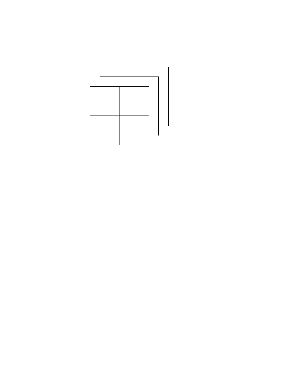
A. & A. Borovik • Mirrors and Reflections • Version 01 • 25.02.00
73
r
1
r
1
r
1
r
1
r
1
r
1
r
3
r
2
r
3
r
2
r
3
r
2
r
3
r
2
r
3
r
2
r
3
r
2
r
3
r
2
r
3
r
2
r
3
r
2
r
3
r
2
r
3
r
2
r
3
r
2
H
H
H
H
H
H
H
H
H
A
A
A
A
A
A
A
A
A
@
@
@
@
@
@
@
@
@
@
@
@
@
Figure 3.7:
Labelling of panels in the Coxeter complex BC
3
.
3.6
Labelling of the Coxeter complex
We shall use the simple transitivity of the action of the reflection group
W on its Coxeter complex C to label each panel of the Coxeter complex C
with one of the simple reflections r
1
, . . . , r
n
; the procedure for labelling is
as follows.
First we label the panels of the fundamental chamber C by the corre-
sponding simple reflections. If D is a chamber in C, then there is unique
element w ∈ W which sends C to D = wC. If Q is a panel of D, we assign
to the panel Q of D the same label as that of the panel P = w
−1
Q of C.
However, we need to take care of consistency of labelling: the panel Q
belongs to two adjacent chambers D and D
0
. If we label the panels of D
0
by the same rule, will the label assigned to Q be the same? Let r be the
simple reflection in the panel P and C
0
= rC the chamber adjacent to C
and sharing the panel P with C. Since the action of W on C preserves
adjacency of chambers, D
0
= wC
0
= wrC. Hence wr is a unique element
of W which send C to D
0
, and we assign to the panel Q the label of the
panel (wr)
−1
Q of C. But rP = P , hence (wr)
−1
Qrw
−1
Q = rP = P , and
Q gets the same label as before.
If a common panel of two chambers D and E is labelled r
i
, we shall
say that D and E are r
i
-adjacent . This includes the case D = E, so that
every chamber is r
i
-adjacent to itself.
The following observation is immediate.
Proposition 3.6.1 The action of W preserves the labelling of panels in

74
the Coxeter complex C.
Moreover, we can now start to develope a vocabulary for translation of
the geometric properties of the Coxeter complex C into the language of the
corresponding reflection group W .
Theorem 3.6.2 Let C be a fundamental chamber in the Coxeter complex
C of a reflection group W . The map
w 7→ wC
is a one-to-one correspondence between the elements in W and chambers
in C. Two distinct chambers C and C
0
are r
i
-adjacent if and only if the
corresponding elements w and w
0
are related as w
0
= wr
i
.
Now the description of canonical galleries given in Theorems 3.4.1 and
3.4.2 can be put in a much more convenient form.
Let Γ = { C
0
, . . . , C
l
} be a gallery and let r
i
k
the label of the common
panel of the consequent chambers C
k−1
and C
k
, k = 1, . . . , l. Then we say
that Γ has type r
i
1
, . . . , r
i
l
.
Theorem 3.6.3 Let Γ = { C
0
, . . . , C
l
} be a gallery of type r
i
1
, . . . , r
i
l
con-
necting the fundamental chamber C = C
0
and a chamber D = C
l
. Set
ˆ
r
i
k
=
r
i
k
if C
k−1
6= C
k
1
if C
k−1
= C
k
.
Then
D = ˆ
r
i
1
· · · ˆr
i
l
C.
For all k = 1, . . . , l, the element of W corresponding to the chamber C
k
is
ˆ
r
i
1
· · · ˆr
i
k
. In particular, if the galery Γ does not stutter, then we have, for
all k, ˆ
r
i
k
= r
i
k
and Γ is a canonical gallery for the word w = r
i
1
· · · r
i
l
.
Proof.
The proof is obvious.
3.7
Isotropy groups
We remain in the standard setting of our study: Φ is a root system in
R
n
,
Σ is the corresponding mirror system and W is the reflection group.
If α is a vector in
R
n
, its isotropy group or stabiliser , or centraliser (all
these terms are used in the literature) C
W
(α) is the group
C
W
(α) = { w ∈ W | wα = α };

A. & A. Borovik • Mirrors and Reflections • Version 01 • 25.02.00
75
if X ⊆ R
n
is a set of vectors, then its isotropy group or pointwise centraliser
in W is the group
C
W
(X) = { w ∈ W | wα = α for all α ∈ X }.
Theorem 3.7.1 In this notation,
(1) The isotropy group C
W
(X) of a set X ⊂ R
n
is generated by those re-
flections in W which it contains. In other words, C
W
(X) is generated
by reflections s
H
, H ∈ Σ, whose mirrors contain the set X.
(2) If X belongs to the closure C of the fundamental chamber then the
isotropy group C
W
(X) is generated by the simple reflections it con-
tains.
Proof.
Consider first the case when X = { α } consists of one vector.
Write W
0
= C
W
(α). If the vector α does not belong to any mirror in Σ
then it lies in one of the open chambers in C, say D, and wD = D for
any w ∈ W
0
. It follows from the simple transitivity of W on the Coxeter
complex C (Theorem 3.5.1) that W
0
= 1, and the theorem is true since W
0
contains no reflections.
Now denote by Σ
0
the set of all mirrors in Σ which contain α. Obviously,
Σ
0
is a closed mirror system and is invariant under the action of W
0
.
Consider the set C
0
of all chambers D such that α ∈ D. Notice that C
0
is invariant under the action of W
0
.
If D ∈ C
0
and P a panel of D containing α then the wall H of P belongs
to Σ
0
, and the chamber D
0
adjacent to D via the panel P belongs to C
0
.
Also, if two chambers D, D
0
∈ C
0
are adjacent in C and have the panel P
in common, then P = D ∩ D
0
contains α, and the wall H containing the
panel P and its closure P belongs to Σ
0
.
These observations allow us to prove that any two chambers D and D
0
in C
0
can be connected by a gallery which belongs to C
0
. Indeed, let
D = D
0
, D
1
, . . . , D
l
= D
0
be a geodesic gallery connecting D and D
0
. If one of the chambers in the
gallery, say D
k
, does not belong to C
0
, then select the minimal k with this
property and look at the wall H separating D
k−1
and D
k
. The chambers
D, D
k−1
, D
0
lie on the same side of the wall H as the point α. But a
geodesic gallery intersects each wall only once. Hence the entire gallery
belongs to C
0
.
Now take an arbitrary w ∈ W
0
and consider a gallery D
0
, . . . , D
l
in C
0
connecting the chambers D = D
0
and D
l
= wD. If s
i
is the reflection in the

76
common panel of the consecutive chambers D
i−1
and D
i
, i = 1, . . . , l, then
D
0
= s
l
· · · s
1
D. Since W acts on C simply transitively, w = s
l
· · · s
1
. But,
for each i, s
i
∈ W
0
, therefore the group W
0
is generated by the reflections
it contains. This proves (1) in our special case. The statement (2) for
X = {α} follows from the observation that if D = C is the fundamental
chamber then the proof of the Theorem 3.2.1 can be repeated word for
word for W
0
and C
0
and shows that W
0
is generated by reflections in the
walls of the fundamental chamber C, i.e. by simple reflections.
Now consider the general case. If every point in X belongs to every
mirror in Σ then C
W
(X) = W and the theorem is trivially true. Otherwise
take any α in X such that the system Σ
0
of mirrors containing α is strictly
smaller than Σ. Then C
W
(X)
6 C
W
(α) and W
0
= C
W
(α) is itself the
reflection group of Σ
0
. We can use induction on the number of mirrors in
Σ, and application of the inductive assumption to Σ
0
completes the proof.
Exercises
3.7.1 For the symmetry group of the cube ∆ = [−1, 1]
3
, find the isotropy
groups
(a) of a vertex of the cube,
(b) of the midpoint of an edge,
(c) of the center of a 2-dimensional face.
3.7.2 Let Φ be the root system of the finite reflection group W and α ∈ Φ.
Prove that the isotropy group C
W
(α) is generated by the reflections s
β
for all
roots β ∈ Φ orthogonal to α.
3.7.3 The centraliser C
W
(u) of an element w ∈ W is the set of all elements in
W which commute with u:
C
W
(w) = { v ∈ W | vu = uv }.
Let s
α
be the reflection corresponding to the root α ∈ Φ. Prove that
C
W
(s
α
) = hs
α
i × hs
β
| β ∈ Φ and β orthogonal to αi.
3.7.4 Let W = Sym
n
and r = (12). Prove that
C
W
(r) = h(12)i × h(34), (45), . . . , (n − 1, n)i
and is isomorhic to Sym
2
× Sym
n−2
.

A. & A. Borovik • Mirrors and Reflections • Version 01 • 25.02.00
77
3.7.5 Let ∆ be a convex polytope and assume that its group of symmetries
contains a subgroup W generated by reflections. If Γ is a face of ∆, prove that
the set-wise stabiliser of Γ in W
Stab
W
(Γ) = { w ∈ W | wΓ = Γ }
is generated by reflections.
3.8
Parabolic subgroups
Let Π be a simple system in the root system Φ and r
1
, . . . , r
m
the cor-
responding system of simple reflections. Denote I = { 1, . . . , m, }. For a
subset J ⊆ I denote
W
J
= hr
i
| i ∈ Ji;
subgroups W
J
are called standard parabolic subgroups of W . Notice W
I
=
W and W
∅
= 1.
For each i = 1, . . . , m, denote by P
i
the (closed) panel of the closed
fundamental chamber C corresponding to the reflection r
i
, and set
P
J
=
\
i∈J
P
J
.
By virtue of Theorem 3.7.1,
W
J
= C
W
(P
J
).
We are now in a position to obtain a very easy proof of the following
beautiful properties of parabolic subgroups.
Theorem 3.8.1 If J and K are subsets of I then
W
J ∪K
= hW
J
, W
K
i
and
W
J ∩K
= W
J
∩ W
K
.
Proof.
The first equality is obvious, the second one follows from the
observation that
W
J
∩ W
K
= C
W
(P
J
) ∩ C
W
(P
K
) = C
W
(P
J
∪ P
K
)

78
By Theorem 3.7.1, the latter group is generated by those simple reflections
whose mirrors contain the both sets P
J
and P
K
, that is, by reflections r
i
with i ∈ J ∩ K. Therefore
W
J ∩K
= W
J
∩ W
K
.
In particular, this theorem means that
{ r
1
, . . . , r
n
} ∩ W
J
= { r
i
| i ∈ J }.
We have an important geometric interpretation of this result.
Proposition 3.8.2 Let D and E be the chambers corresponding to the
elements u and v of a parabolic subgroup P
J
. If D and E are r
j
-adjacent
then j ∈ J.
Proof.
Since D and E are r
j
-adjacent, then, by Theorem 3.6.2, we have
ur
j
= v and r
j
∈ P
J
. Therefore j ∈ J.
Exercises
3.8.1 Let W = A
n−1
and let us view W as the symmetric group Sym
n
of the
set [n], so that the simple reflections in W are
r
1
= (12), r
2
= (23), . . . r
n−1
= (n − 1, n).
Prove that the parabolic subgroup
P = hr
1
, . . . , r
k−1
, r
k+1
, . . . , r
n−1
i
is the stabiliser in Sym
n
of the set { 1, . . . , k } and thus is isomorphic to Sym
k
×
Sym
n−k
.
3.9
Residues
We retain the notation of the previous sections.
Let D be a chamber in C and J ⊂ I. A J-residue of D is the set of all
chambers in C which can be connected to D by galleries in which types of
panels between consequent chambers are of type r
i
for i ∈ J.
Let C be the fundamental chamber of C and w the element of W which
canonically corresponds to D, that is, D = wC. Then Theorem 3.6.3
says that a chamber vC belongs to the J -residue of D if and only if v =
wr
i
1
· · · r
i
t
with i
1
, . . . , i
t
∈ J. Now we have to recall the definition of a
parabolic subgroup P
J
= hr
i
| i ∈ Ji and conclude that the chamber vC
belongs to the J -residue of D = wC if and only if v ∈ wP
J
. Therefore
J -residues are in one-two-one correspondence with the left cosets of the
parabolic subgroup P
J
.
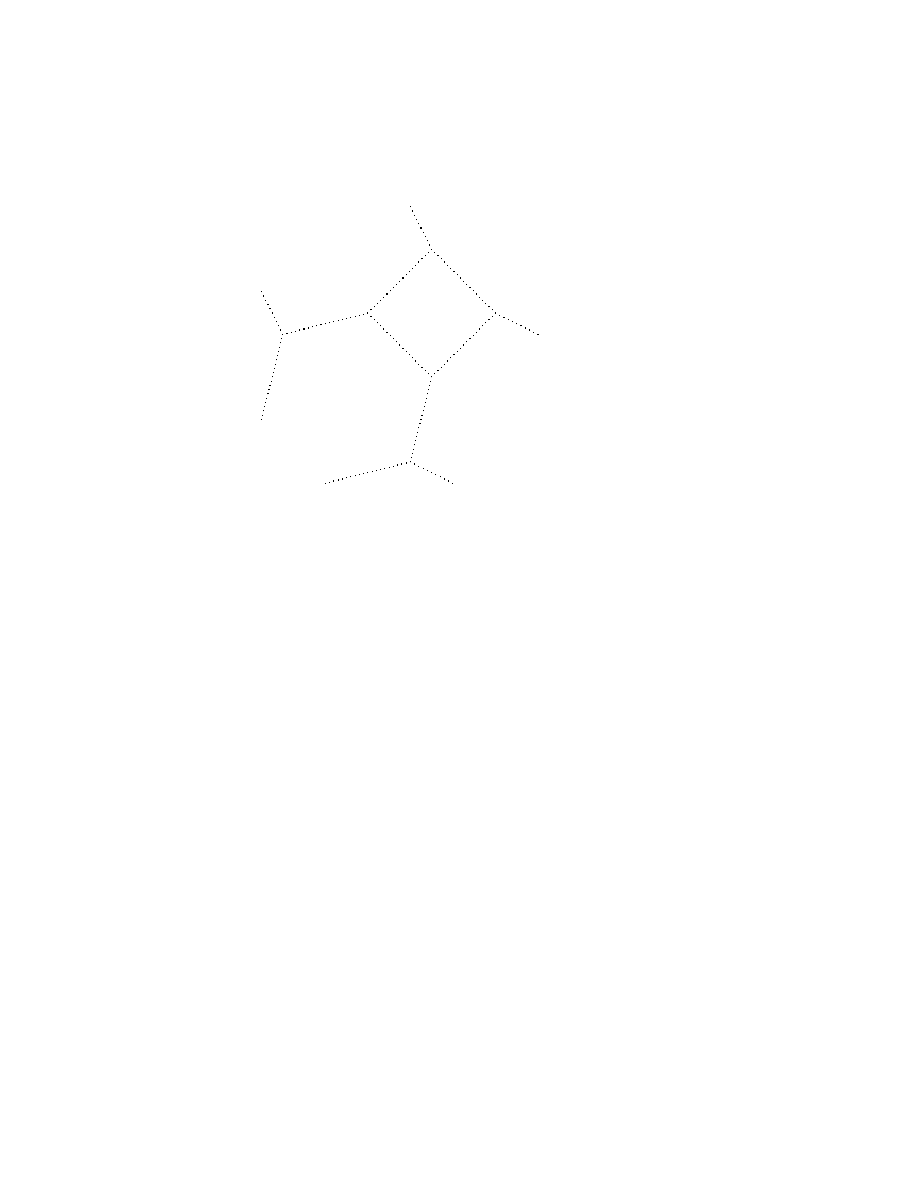
A. & A. Borovik • Mirrors and Reflections • Version 01 • 25.02.00
79
H
HH
A
A
A
@
@
@
@
@
H
HH
@
@
@
@
@
H
H
H
A
A
A
@
@
@
@
@
A
A
A
A
A
A
@
@
@
@
@
H
HH
[1234]
[1243]
[2143]
[2134]
[1423]
[1432]
[4132]
[4123]
[1324]
[3124]
[3142]
[1342]
[2413]
[4213]
[4231]
[2431]
[4321]
[4312]
[3412]
[3421]
[2314]
[2341]
[3241]
[3214]
Figure 3.8:
A permutahedron for the group A
3
= Sym
4
. Its vertices form
one orbit under the permutation action of Sym
4
in
R
3
and can be labelled by
elements of Sym
4
. Here [i
1
i
2
i
3
i
4
] denotes the permutation 1 7→ i
1
, . . . , 4 7→ i
4
.
3.10
Generalised permutahedra
We say that a point α ∈ V is in general position if α does not belong to Σ.
Let now δ be any point in general position, W · δ its orbit under W and
∆ the convex hull of W · δ. We shall call ∆ a generalised permutahedron
and study it in some detail.
Theorem 3.10.1 In the notation above, the following statements hold.
(1) Vertices of ∆ are exactly all points in the orbit W · δ and each chamber
in C contains exactly one vertex of ∆.
(2) Every edge of ∆ is parallel to some vector in Φ and intersects exactly
one wall of the Coxeter complex C.
(3) The edges emanating from the given vertex are directed along roots
forming a simple system.
(4) If α is the vertex of ∆ contained in a chamber C then the vertices
adjacent to α are exactly all the mirror images s
i
α of α in walls of
C.
80
@
@
@
@
@
@
@
@
@
PP
PP
PP
PPP
r
α
r
α
0
r
β
0
r
β
H
ρ
The segment [αβ] not normal to a
mirror H
ρ
it crosses cannot be an
edge of the permutahedron ∆; in-
deed, if α
0
and β
0
are reflections of
α and β in H
ρ
then α
0
and β
0
are
also vertices of ∆ and [αβ] belongs
to the convex hull of α, β, α
0
, β
0
.
Figure 3.9:
For the proof of Theorem 3.10.1.
Proof.
Notice, first of all, that, since all points in the orbit W · δ lie at
the same distance from the origin, they belong to some sphere centered at
the origin. Therefore points in W · δ are the vertices of the convex hull of
W · δ. Next, because of simple transitivity of W on the Coxeter complex
C, every chamber in C contains exactly one vertex of ∆. This proves (1).
Let now α and β be two adjacent, i.e. connected by an edge, vertexes of
∆. Then β belongs to a chamber distinct from α and, therefore, the edge
[αβ] intersects some mirror H
ρ
. If the edge [αβ] is not perpendicular to H
ρ
,
we immediately have a contradiction with the following simple geometric
argument (see Figure 3.9).
In Figure 3.9, the points α
0
and β
0
are symmetric to α, β, respectively, and
the convex quadrangle αα
0
ββ
0
lies in a 2-dimensional plane perpendicular
to the mirror H
ρ
of symmetry. Therefore the segment [αβ] belongs to the
interior of the quadrangle and cannot be an edge of ∆.
Hence [αβ] is perpendicular to H
ρ
, hence β − α = cρ for some c and
the mirror H
ρ
is uniquely determined, which proves (2).
Now, select a linear functional f which attains its minimum on ∆ at
the point α and does not vanish at roots in Φ. Let Φ
+
and Π be the
positive and simple system in Φ associated with f . If s
±ρ
= s
ρ
= s
−ρ
is the reflection in W for the roots ±ρ, then s
±ρ
α is a vertex of ∆ and
f (s
±ρ
α − α) > 0. But s
±ρ
α − α = cρ for some c. After swapping notation
for +ρ and −ρ we can assume without loss that f(ρ) > 0, i.e. ρ ∈ Φ
+
and
c > 0. Let β
1
, . . . , β
m
be all vertices of ∆ adjacent to α. Then β
i
− α = c
i
ρ
i
for some ρ
i
∈ Φ
+
and c
i
> 0.
And here comes the punchline: notice that the convex polytope ∆ is
contained in the convex cone Γ spanned by the edges emanating from α
(Figure 3.10). Since every positive roots ρ ∈ Φ
+
points from the vertex α
to the vertex s
ρ
α of ∆, all positive roots lie in the convex cone spanned by
A. & A. Borovik • Mirrors and Reflections • Version 01 • 25.02.00
81
@
@
@
@
@
@
@
@
@
@
J
J
J
J
J
J
J
H
H
H
HH
H
H
H
HH
H
H
(( (
(
(((
(
@
@
@
H
H
J
J
J
J
(((
(
H
H
One of the simple principles of
linear programming which is ex-
tremely useful in the study of Cox-
eter groups: a convex polytope is
contained in the convex polyhedral
cone spanned by the edges emanat-
ing from the given vertex.
Figure 3.10: For the proof of Theorem 3.10.1.
the roots ρ
i
∈ Φ
+
pointing from α to adjacent to α vertices β
i
. But this
means exactly that ρ
i
form the simple system Π in Φ
+
, which proves (3).
Also, the fact that β
i
− α = cρ
i
for c > 0 means that α ∈ V
−
ρ
i
. Since this
holds for all simple roots, α belongs to the fundamental chamber C =
T
V
−
ρ
i
(Theorem 3.1.1). But, by the same theorem, C is bounded by the mirrors
of simple reflections and β
i
= s
ρ
i
α is the mirror image of α in the wall H
ρ
i
containing a panel of C. (4) is also proven.
Exercises
3.10.1 Sketch permutahedra for the reflection groups
A
1
+ A
1
, A
2
, BC
2
, A
1
+ A
1
+ A
1
, A
2
+ A
1
.
3.10.2 Label, in a way analogous to Figure 3.8, the vertices of a permutahedron
for the hyperoctahedral group BC
3
(Figure 3.11) by elements of the group.
3.10.3 Let ∆ be a permutahedron for a reflection group W . Prove that there
is a one-to-one correspondence between faces of ∆ and residues in the Coxeter
complex C of W . Namely, the set of chambers containing vertices of a given face
is a residue.
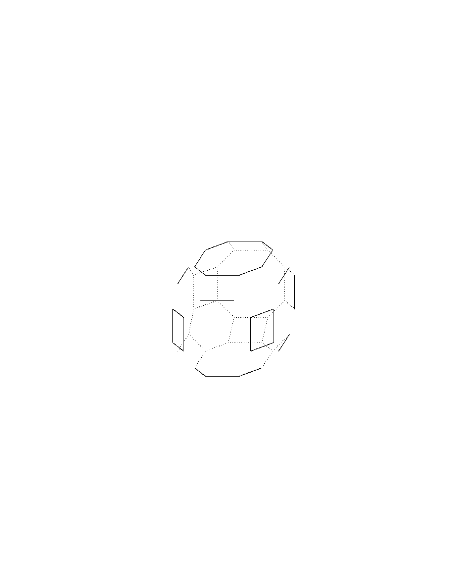
82
@
@
@
@
@
@
@
@
@
@
@
@
@
@
@
T
T
T
T
T
T
T
T
T
T
Figure 3.11:
A permutahedron for BC
3
(Exercise 3.10.2).

Chapter 4
Classification
4.1
Generators and relations
Let W be a finite reflection group and R = {r
1
, . . . , r
m
} the set of simple
reflections in W . Denote m
ij
= |r
i
r
j
|. Notice m
ii
= 1 for all i.
Theorem 4.1.1 The group W is given by the following generators and
relations:
W = hr
1
, . . . , r
m
| (r
i
r
j
)
m
ij
= 1i.
Proof.
4.2
Decomposable reflection groups
Coxeter graph.
By Theorem 4.1.1, a a finite reflection group W is given
by the following generators and relations:
W = hr
1
, . . . , r
m
| (r
i
r
j
)
m
ij
= 1i
where R = {r
1
, . . . , r
m
} is the set of simple reflections in W and m
ij
=
|r
i
r
j
|. Notice m
ii
= 1 for all i.
Now we wish to associate with W and a system of simple reflections
R a graph G, called Coxeter graph, whose nodes are in one-to-one cor-
respondence with the simple reflections r
1
, . . . , r
n
in R. If r
i
and r
j
are
two distinct reflections, then, if m
ij
= |r
i
r
j
| > 2, the nodes r
i
and r
j
are
connected by an edge with mark m
ij
on it. If m
ij
= 2, that is, if r
i
and
r
j
commute, then there is no edge connecting r
i
and r
j
. We say that the
group W is indecomposable if the graph G is connected; otherwise W is
said to be decomposable.
83
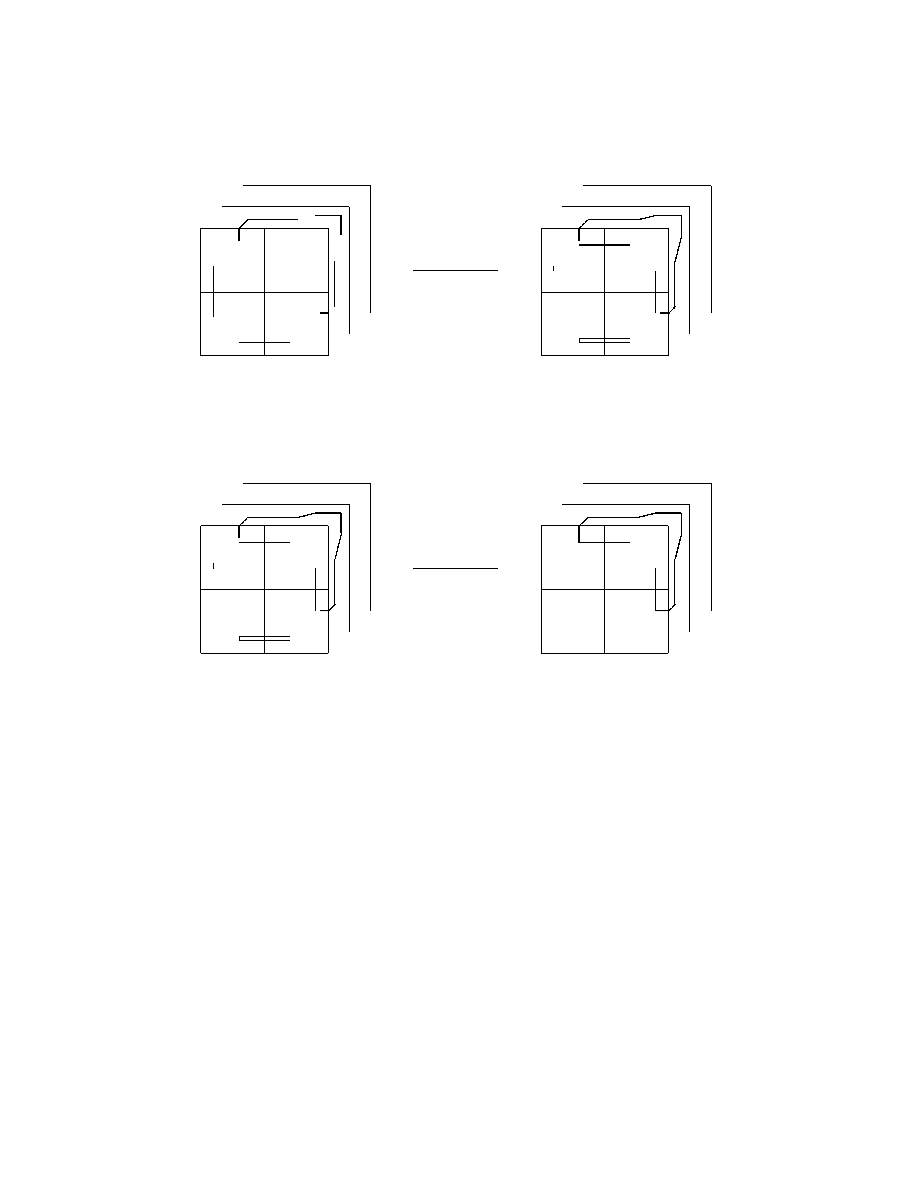
84
1
1
-
r
3
r
2
r
2
?
-
9
6
-
@
@
R
?
?
9
6
-
@
@
R
?
H
H
H
H
HH
H
H
H
H
HH
H
H
H
H
H
H
A
A
A
A
A
A
@
@
@
@
@
@
@
@
@
H
H
H
H
H
H
A
A
A
A
A
A
@
@
@
@
@
@
@
@
@
1
1
-
r
3
r
2
9
?
?
@
@
R
-
6
?
-
9
6
-
@
@
R
?
H
H
H
H
HH
H
H
H
H
HH
H
H
H
H
H
H
A
A
A
A
A
A
@
@
@
@
@
@
@
@
@
H
H
H
H
H
H
A
A
A
A
A
A
@
@
@
@
@
@
@
@
@
D
Removing a chamber D from a circular gallery. Here we use the relation
r
3
r
2
= r
2
r
3
r
2
r
3
r
2
r
3
which is a consequence of (r
2
r
3
)
4
= 1.
Removing dead end and repeated chambers from a circular gallery. We use
the relations r
2
2
= r
2
3
= 1.
Figure 4.1:
For the proof of Theorem 4.1.1.
Theorem 4.2.1 Assume that W is decomposable and let G
1
, . . . , G
k
be
connected components of G. Let R
j
be the set of reflections corresponding
to nodes in the connected component G
j
, j = 1, . . . , k. Let W
j
be the
parabolic subgroup generated by the set R
j
. Then
W = W
1
× · · · × W
k
.
Proof.
If i 6= j then any two reflections r
0
∈ R
i
and r
00
∈ R
j
commute,
hence
• the subgroups W
i
= hR
i
i and W
j
= hR
j
i commute elementwise.
By Theorem 3.8.1, the intersection of W
j
with the group generated by all
W
i
with i 6= j is the subgroup generated by R
j
∩
S
i6=j
R
i
= ∅, that is, the
identity subgroup:

A. & A. Borovik • Mirrors and Reflections • Version 01 • 25.02.00
85
• W
j
∩ hW
1
, . . . , c
W
j
, . . . , W
k
i = 1.
Finally, the subgroups W
i
generate W ,
• W = hW
1
, . . . , W
k
i.
But these properties of the subgroups W
i
mean exactly that
W = W
1
× · · · × W
k
.
4.3
Classification of finite reflection groups
4.4
Construction of root systems
In this section we shall construct, for each Coxeter graph of type
A
n
, B
n
, C
n
, D
n
, E
6
, E
7
, E
8
, F
4
, G
2
a root system. An immediate computation shows that all these systems are
crystallographic. We do not consider the root systems of type H
3
and H
4
.
The interested reader may wish to consult the books [GB] and [H] which
contain a detailed discussion of these non-crystallographic root systems.
We notice only that the mirror system associated with the root system of
type H
3
is the system of mirrors of symmetry of the regular icosahedron.
Root system A
n
.
Let
1
, . . . ,
n+1
be the standard basis in
R
n+1
.
Φ = {
i
−
j
| i, j = 1, . . . , n + 1, i 6= j },
Π = {
2
−
1
, . . . ,
n+1
−
n
}.
Φ contains n(n + 1) vectors, all of whose are of equal length. Denote the
simple vectors as
ρ
1
=
2
−
1
, ρ
2
=
3
−
2
, . . . , ρ
n
=
n+1
−
n
and take the root
ρ
0
=
n+1
−
1
= ρ
1
+ ρ
2
+ · · · + ρ
n
.
The root ρ
0
is called the highest root because it has, of all positive roots,
the longest expression in terms of the simple roots. The highest root plays

86
an exceptionally important role in many applications of the theory of root
systems, for example, in the representation theory of simple Lie algebras
and simple algebraic groups.
In the following diagram the black nodes form the Coxeter graph for
A
n
; an extra white node demonstrates the relations of the root −ρ
0
to the
simple roots. We use the following convention: if α and β are two roots,
then their nodes are not connected if (α, β) = 0 (and the reflections s
α
and
s
β
commute), and the nodes are connected by an edge if
(α, β)
|α||β|
= − cos
π
m
and m
> 3. In fact, m is the order of the product s
α
s
β
and m
> 3 if and
only if the reflections s
α
and s
β
do not commute. If m > 3 we write the
mark m on the edge.
s
s
. . .
s
s
c
ρ
1
ρ
2
ρ
n
ρ
n−1
−ρ
0
We know that the reflection group W for our root system is the sym-
metric group Sym
n+1
which acts by permuting the vectors
i
.
Root system B
n
, n
> 2. Let
1
, . . . ,
n
be the standard basis in
R
n
.
Φ = { ±
i
, ±
i
± e
j
| i, j = 1, . . . , n, i < j },
Π = {
1
,
2
−
1
, . . . ,
n
−
n−1
}.
Φ contains 2n short roots ±
i
and 2n(n − 1) long roots ±
i
±
j
, i < j.
It is convenient to enumerate the simple roots as
ρ
1
=
1
, ρ
2
=
2
−
1
, . . . , ρ
n
=
n
−
n−1
.
The highest root is
ρ
0
=
n−1
+
n
.
The extended Coxeter diagrams for the system of roots B
2
and B
n
with
n
> 3 look differently.
s
s
4
4
c
−ρ
0
ρ
1
ρ
2

A. & A. Borovik • Mirrors and Reflections • Version 01 • 25.02.00
87
Extended Coxeter diagram for B
2
s
s
s
. . .
s
s
H
H
H
4
c
ρ
3
ρ
1
ρ
2
ρ
n
ρ
n−1
−ρ
0
Extended Coxeter diagram for B
n
, n
> 3.
Root system C
n
, n
> 2. Let
1
, . . . ,
n
be the standard basis in
R
n
.
Φ = { ±2
i
, ±
i
± e
j
| i, j = 1, . . . , n, i < j },
Π = { 2
1
,
2
−
1
, . . . ,
n
−
n−1
}.
Φ contains 2n long roots ±2
i
and 2n(n − 1) short roots ±
i
±
j
, i < j.
We enumerate the simple roots as
ρ
1
= 2
1
, ρ
2
=
2
−
1
, . . . , ρ
n
=
n
−
n−1
.
The highest root is
ρ
0
= 2
n
.
s
s
4
4
c
−ρ
0
ρ
1
ρ
2
Extended Coxeter diagram for C
2
s
s
s
. . .
s
s
4
c
ρ
3
ρ
1
ρ
2
ρ
n
ρ
n−1
4
−ρ
0
Extended Coxeter diagram for C
n
, n
> 3.
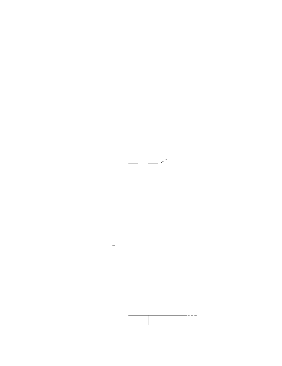
88
Root system D
n
, n
> 4. Let
1
, . . . ,
n
be the standard basis in
R
n
.
Φ = { ±
i
±
j
| i, j = 1, 2, . . . , n, i 6= j };
thus D
n
is a subsystem of the root system C
n
. All roots have the same
length. The total number of roots is 2n(n − 1).
The simple system Π is
ρ
1
=
1
+
2
, ρ
2
=
2
−
1
, ρ
3
=
3
−
2
, . . . , ρ
n
=
n
−
n−1
The highest root is
ρ
0
=
n−1
+
n
.
H
H
H
s
s
s
s
. . .
s
sH
H
H
c
s
−ρ
0
ρ
1
ρ
2
ρ
3
ρ
n−2
ρ
n−1
ρ
n
Root system E
8
.
Let
1
, . . . ,
8
be the standard basis in
R
8
.
Φ =
(
±
i
± e
j
(i < j),
1
2
8
X
i=1
±
i
(even number of + signs)
)
,
for Π take
ρ
1
=
1
2
(
1
−
2
−
3
−
4
−
5
−
6
−
7
+
8
),
ρ
2
=
1
+
2
,
ρ
i
=
i−1
−
i−2
(3
6 i 6 8).
All roots have the same length; the total number of roots is 240.
The highest root is
ρ
0
=
7
+
8
.
s
s
s
s
s
s
s
s
c
−ρ
0
ρ
1
ρ
2
ρ
3
ρ
4
ρ
5
ρ
6
ρ
7
ρ
8

A. & A. Borovik • Mirrors and Reflections • Version 01 • 25.02.00
89
Root system E
7
.
Take the root system of type E
8
in
R
8
just constructed
and consider the span V of the roots ρ
1
, . . . , ρ
7
. Let Φ be the set of 126
roots of E
8
belonging to V :
±
i
±
j
(1
6 i < j 6 6),
±(
7
−
8
),
±
1
2
7
−
8
+
6
X
i=1
±
i
!
,
where the number of minus signs in the sum is odd.
All roots have the same length. The roots
ρ
1
, . . . , ρ
7
form a simple system, and the highest root is
ρ
0
=
8
−
7
.
c
s
s
s
s
s
s
s
−ρ
0
ρ
1
ρ
2
ρ
3
ρ
4
ρ
5
ρ
6
ρ
7
Root system E
6
.
Again we start with the root system of type E
8
in
R
8
.
Denote by V the span of the roots ρ
1
, . . . , ρ
6
, and take for Φ the 72 roots
of E
8
belonging to V :
±
i
±
j
(1
6 i < j 6 5),
±
1
2
8
−
7
−
6
+
5
X
i=1
±
i
!
,
where the number of minus signs in the sum is odd.
All roots have the same length. The roots
ρ
1
, . . . , ρ
6
form a simple system, and the highest root is
ρ
0
=
1
2
(
1
+
2
+
3
+
4
+
5
−
6
−
7
+
8
).
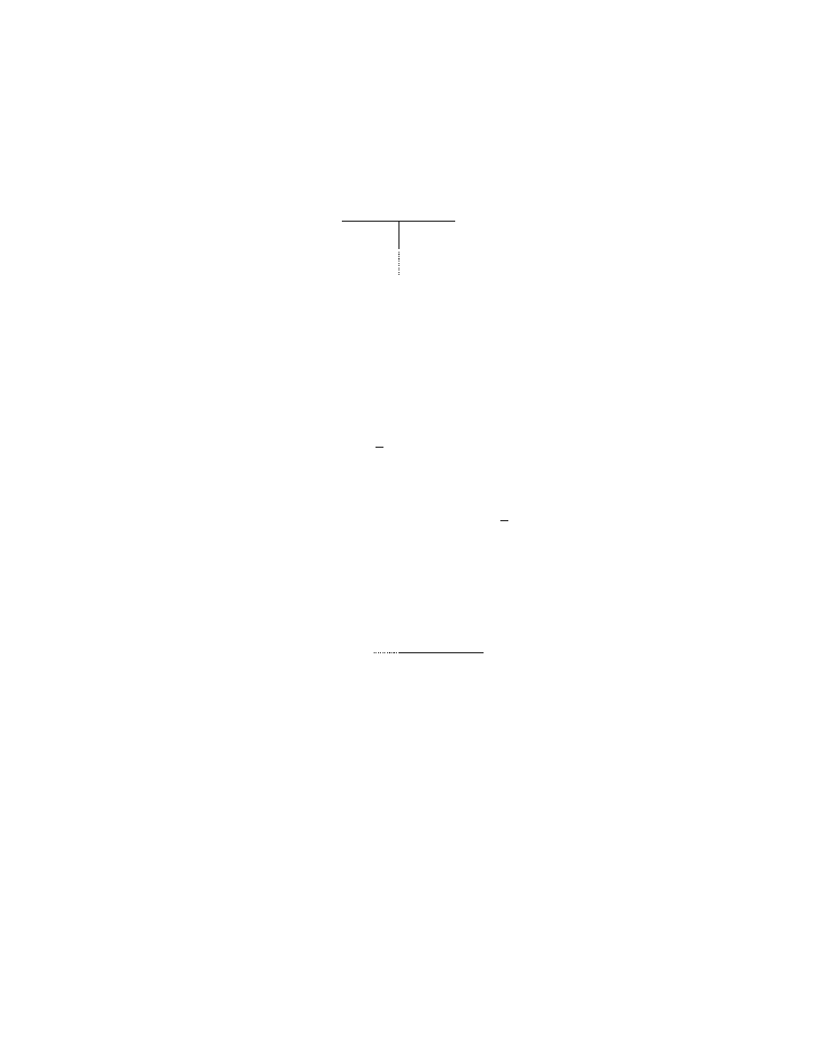
90
s
s
s
s
s
s
c
−ρ
0
ρ
1
ρ
2
ρ
3
ρ
4
ρ
5
ρ
6
Root system F
4
.
Let
1
, . . . ,
4
be the standard basis in
R
4
. Φ consists
of 24 long roots
±
i
±
j
(i < j)
and 24 short roots
±
i
,
1
2
(±
1
±
2
±
3
±
4
).
For a simple system Π take
ρ
1
=
2
−
3
, ρ
2
=
3
−
4
, ρ
3
=
4
, ρ
4
=
1
2
(
1
−
2
−
3
−
4
).
The highest root is
ρ
0
=
1
+
2
.
c
s
s
s
s
4
ρ
0
ρ
1
ρ
2
ρ
3
ρ
4
Root system G
2
.
Let V be the hyperplane x
1
+ x
2
+ x
3
= 0 in
R
3
. Φ
consists of 6 short roots
±(
i
−
j
),
i < j,
and 6 long roots
±(2
i
−
j
−
k
),
where i, j, k are all different. For a simple system Π take
ρ
1
=
1
−
2
, ρ
2
= −2
1
+
2
+
3
.
The highest root is
ρ
0
=
1
+
2
.

A. & A. Borovik • Mirrors and Reflections • Version 01 • 25.02.00
91
s
s
6
c
−ρ
0
ρ
1
ρ
2
Exercises
For every of the root systems A
n
, B
n
, C
n
, D
n
, E
6
, E
7
, E
8
, F
4
, G
2
:
4.4.1 Check the crystallographic condition.
4.4.2 Find the decomposition of the highest root with respect to the simple
roots.
4.4.3 Check, by a direct computation, that the extended Coxeter diagrams are
drawn correctly.
4.4.4 The sets Φ
long
and Φ
short
of all long (correspondingly, short) roots in a
root system Φ are root systems on their own. Identify their types when Φ is ot
type B
n
, C
n
or F
4
.
4.5
Orders of reflection groups
In this section we shall use information about the root systems accumulated
in Section 4.4 to determine the orders of the finite reflection groups
A
n
, BC
n
, D
n
, E
6
, E
7
, E
8
F
4
G
2
.
Notice that the group A
1
, obviously, has order 2. The groups A
2
, BC
2
,
G
2
are the dihedral groups of orders 6, 8, 12, correspondingly.
Let Φ be one of the root systems listed above and W its reflection
group. To work out the order of W we need first to study the action of W
on Φ.
Lemma 4.5.1 The long (respectively, short ) roots in Φ are conjugate un-
der the action of W .

92
Proof.
We know from Theorem 3.5.6 that every root is conjugate to a
simple root. Therefore it will be enough to prove that the simple long
(respectively, short) roots are conjugate. Direct observation of Coxeter
graphs shows that the nodes for any two simple roots of the same length
can be connected by a sequence of edges with marks 3. Hence it will be
enough to prove that if ρ
i
and ρ
j
are distinct simple roots so that m
ij
= 3
then ρ
i
and ρ
j
are conjugate.
Since the system of simple roots is linearly independent, the set Φ
0
=
Φ ∩(Zρ
i
+
Zρ
j
) consists of those vectors in Φ which are linear combinations
of ρ
i
and ρ
j
. We have already checked, on several occasions, that Φ
0
is
a root system and { ρ
i
, ρ
j
} is a simple system in Φ
0
. The corresponding
reflection group W
0
is a dihedral group of order 6. One can see immediately
from a simple diagram that all roots in Φ
0
form a single W
0
-orbit (check
this!). Alternatively, we can argue as follows
1
: reflections in W
0
are in one-
to-one correspondence with the 3 pairs of opposite roots in Φ
0
. But W
0
contains exactly 3 involutions, hence every involution in W
0
is a reflection.
Every reflection in W
0
generates a subgroup of order 2 which is a Sylow 2-
subgroup in W
0
. By Sylow’s Theorem, all Sylow 2-subgroups are conjugate
in W
0
, hence all reflections are conjugate in W
0
, hence all pairs of opposite
roots in Φ
0
are conjugate, hence all roots in Φ
0
are conjugate in W
0
and,
since W
0
< W , in W .
Theorem 4.5.2 The orders of the indecomposable reflection groups are
given in the following table.
|A
n
| = n!
|BC
n
| = 2
n
· n!
|D
n
| = 2
n−1
· n!
|E
6
| = 2
7
· 3
4
· 5
|E
7
| = 2
10
· 3
4
· 5 · 7
|E
8
| = 2
14
· 3
5
· 5
2
· 7
|F
4
| = 2
7
· 3
2
|G
2
| = 12
Proof.
In all cases the highest root ρ
0
is a long root. Since all long roots
are conjugate,
|W | =
number
of long
roots
· |C
W
(ρ
0
)|.
1
Which is, essentially, part of the solution to Exercise ??

A. & A. Borovik • Mirrors and Reflections • Version 01 • 25.02.00
93
On the other hand, C
W
(ρ
0
) = C
W
(−ρ
0
). One can easily check, using the
formulae of Section 4.4, that (ρ
0
, ρ
i
)
> 0 for all simple roots ρ
i
, hence
(−ρ
0
, ρ
i
)
6 0 and the root −ρ
0
belons to the closed fundamental chamber
C. By Theorem 3.7.1, the isotropy group C
W
(−ρ
0
) is generated by the
simple reflections which fix the root −ρ
0
. These simple reflections are
exactly the reflections for the black nodes on the extended Coxeter graphs
in Section 4.4 which are not connected by an edge to the white node −ρ
0
.
Therefore the extended Coxeter graph, with the node −ρ
0
and the nodes
adjacent to −ρ
0
deleted, is the Coxeter graph for W
0
= C
W
(ρ
0
), which
allows us to determine the isomorphism type and the order of W
0
.
The rest is a case-by-case analysis.
A
n
. We know that |A
1
| = 2 = 2! and |A
2
| = 6 = 3!. We want to prove
by induction that |A
n
| = (n + 1)!. Φ contains n(n + 1) roots (all of them
of the same length), and W
0
is of type A
n−2
. By the inductive assumption,
|W
0
| = [(n − 2) + 1]! = (n − 1)! and
|W | = n(n + 1) · (n − 1)! = (n + 1)!.
Of cource, we know that W = Sym
n+1
, and there was no much need
in a new proof of the fact that |Sym
n
| = n!. But we wished to use an
opportunity to show how much information about a reflection group is
contained in its extended Coxeter graph.
BC
n
. We know that the root systems B
n
and C
n
have the same mirror
system and reflection group. It will be more convenient for us compute with
the root system C
n
. It contains 2n long roots, and the Coxeter graph for
W
0
is of type C
n−1
. Thus
|W | = 2n · 2
n−1
(n − 1)! = 2
n
n!.
D
n
. All roots are long, and their number is 2n(n − 1). The group W
0
has disconnected Coxeter graph with connected components of types D
n−2
and A
1
, hence W
0
= W
00
× W
000
, where W
00
is of type D
n−2
has, by the
inductive assumption, order 2
n−3
(n − 2)!, and |W
000
| = 2. Therefore
|W | = 2n(n − 1) · (2
n−3
(n − 2)! · 2) = 2
n−1
n!.
E
6
. There are 72 roots in Φ, all of them long; the isotropy group W
0
is of type A
5
. Therefore
|W | = 72 · (5 + 1)! = 72 · 6! = 2
7
· 3
4
· 5.
E
7
. There are 126 roots in Φ, all of them long; the isotropy group W
0
is of type D
6
and has order 2
5
· 6!. Therefore
|W | = 126 · 2
5
· 6! = 2
10
· 3
4
· 5 · 7.

94
E
8
. There are 240 roots in Φ, all of them long; the isotropy group W
0
is of type E
7
and has order 2
10
· 3
4
· 5 · 7 (just computed). Therefore
|W | = 240 · 2
10
· 3
4
· 5 · 7 = 2
14
· 3
5
· 5
2
· 7.
F
4
. There are 24 long roots; the isotropy group W
0
is of type C
3
and
has order 2
3
· 3!. Therefore
|W | = 24 · 2
3
· 3! = 2
7
· 3
2
.
Exercises
4.5.1 Prove that the roots in the root systems H
3
and H
4
form a single orbit
under the action of the corresponding reflection groups.
4.5.2 Lemma 4.5.1 is not true when the root system Φ is not indecomposable.
Give an example.
4.5.3 Give an example of a root system of type A
1
× A
1
× A
1
with roots of
three dfferent lengths.

Bibliography
[A]
M. A. Armstrong, Groups and Symmetry, Springer-Verlag,
1988.
[Ber]
M. Berger, G´
eom´
etrie, Nathan, 1990.
[Bou]
N. Bourbaki, Groupes et Algebras de Lie, Chap. 4, 5, et 6,
Hermann, Paris, 1968.
[G]
B. Gr¨
unbaum, Convex Polytopes, Interscience Publishers, New
York a.o., 1967.
[GB]
L. C. Grove, C. T. Benson, Finite Reflection Groups, Springer-
Verlag, 1984.
[H]
J. E. Humphreys, Reflection Groups and Coxeter Groups,
Cambridge University Press, 1990.
[Roc]
R. T. Rockafellar, Convex Analysis, Princeton Univerity Press,
1970.
[Ron] M. Ronan, Lectures on Buildings, Academic Press, Boston,
1989.
[S]
A. Schrijver, Theory of Linear and Integer Programming,
John Wiley and Sons, Chichester a. o., 1986.
[T]
J. Tits, A local approach to buildings, in The Geometric Vein
(Coxeter Festschrift), Springer-Verlag, New York a.o., 1981,
317–322.
95
Wyszukiwarka
Podobne podstrony:
Kollar The Topology of Real & Complex Algebraic Varietes [sharethefiles com]
Lusztig Some remarks on supercuspidal representations of p adic semisimple groups (1979) [sharethef
Foucault Discourse and Truth The Problematization of Parrhesia (Berkeley,1983)
Pride and Prejudice The Theme of Pride in the Novel
Barbara Stallings, Wilson Peres Growth, Employment, and Equity; The Impact of the Economic Reforms
Piotr Siuda Between Production Capitalism and Consumerism The Culture of Prosumption
Palais R S The geometrization of physics (Tsin Hua lectures, 1981)(107s)
Zinc, diarrhea, and pneumonia The Journal of Pediatrics, December 1999, Vol 135
Mercy and Liberality The Aftermath of the 1569 Northern Rebellion
Shel Leanne, Shelly Leanne Say It Like Obama and WIN!, The Power of Speaking with Purpose and Visio
Subject Positions and Interfaces The Case of European Portuguese
Anatoly Karpov, Jean Fran Phelizon, Bachar Kouatly Chess and the Art of Negotiation Ancient Rules f
Eleswarapu And Venkataraman The Impact Of Legal And Political Institutions On Equity Trading Costs A
Eleswarapu, Thompson And Venkataraman The Impact Of Regulation Fair Disclosure Trading Costs And Inf
Fishea And Robeb The Impact Of Illegal Insider Trading In Dealer And Specialist Markets Evidence Fr
Frino, Mcinish And Toner The Liquidity Of Automated Exchanges New Evidence From German Bund Futures
6482 Ask find and act�harnessing the power of Cortana and Power BI Article
więcej podobnych podstron