Zad. 1. Poniżej przedstawiono wyniki oszacowania liniowego modelu trendu kursu Euro w postaci wydruku komputerowego 1 (z programu Mfit).
Przeprowadź weryfikację modelu ze względu na ocenę dopasowania, istotność parametrów strukturalnych, autokorelację składnika losowego i pozostałe testy diagnostyczne (dl=1,393 du=1,514)
Przedstaw model w postaci po oszacowaniu i zintepretuj go
Zaprognozuj na jego podstawie kurs 100 Euro na grudzień roku 2003
Określ dopuszczalność prognozy, za pomocą średniego błędu predykcji ex-ante (PLN,%) [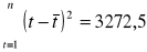
]
Znając realizację grudniową kursu (465,47 PLN) określ trafność prognozy punktowej - błąd ex-post (PLN,%)
Na podstawie błędu ex-ante zbuduj prognozę przedziałową kursu Euro na grudzień 2003 (wartość statystyki t = 2,079)
Ordinary Least Squares Estimation
******************************************************************************
Dependent variable is ECU
34 observations used for estimation from 2001M2 to 2003M11
******************************************************************************
Regressor Coefficient Standard Error T-Ratio[Prob]
C 304.8276 6.8142 44.7340[.000]
T 4.5828 .28467 16.0987[.000]
******************************************************************************
R-Squared .92504 R-Bar-Squared .92148
S.E. of Regression 9.0559 F-stat. F( 1, 21) 259.1676[.000]
Mean of Dependent Variable 410.2317 S.D. of Dependent Variable 32.3167
Residual Sum of Squares 1722.2 Equation Log-likelihood -82.2679
Akaike Info. Criterion -84.2679 Schwarz Bayesian Criterion -85.4034
******************************************************************************
******************************************************************************
* Test Statistics * LM Version * F Version
******************************************************************************
* A:Serial Correlation*CHSQ( 12)= 15.7304[.204]*F( 12, 9)= 1.6229[.237]
* B:Functional Form *CHSQ( 1)= .39178[.531]*F( 1, 20)= .34658[.563]
* C:Normality *CHSQ( 2)= 1.3687[.504]* Not applicable
* D:Heteroscedasticity*CHSQ( 1)= 1.8920[.169]*F( 1, 21)= 1.8824[.185]
******************************************************************************
A:Lagrange multiplier test of residual serial correlation
B:Ramsey's RESET test using the square of the fitted values
C:Based on a test of skewness and kurtosis of residuals
D:Based on the regression of squared residuals on squared fitted values
Zad.2. Na podstawie danych dot. połowów ryb (tys.t) w Polsce w latach 1983-1998 oszacowano następujący model trendu: 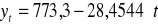
, współczynnik determinacji = 0,93, wariancja resztowa = 1474,55. Czy prognozy na rok 1999 i 2000 wyznaczone za pomocą tego modelu sa dopuszczalne, jeśli ich odbiorca wymaga aby były obarczone błędem nie większym niż 8%? [źródło: Zeliaś A. Prognozowanie ekonomiczne,s.127]
Zad.3. Poniżej przedstawiono wyniki oszacowania wykładniczego modelu trendu przeciętnych wynagrodzeń brutto w postaci wydruku komputerowego 2 (z programu Mfit).
Przeprowadź weryfikację modelu ze względu na ocenę dopasowania, istotność parametrów strukturalnych, autokorelację składnika losowego i pozostałe testy diagnostyczne (dl=0,525 du=2,016)
Przedstaw model w postaci po oszacowaniu i zintepretuj go
Zaprognozuj na jego podstawie wysokość wynagrodzeń na kwartał III i IV roku 2003
Określ dopuszczalność prognoz, za pomocą średniego błędu predykcji ex-ante (PLN,%) [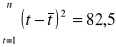
]
Na podstawie błędu ex-ante zbuduj prognozę przedziałową wynagrodzeń na kwartał III roku 2003 (wartość statystyki t = 2,447)
Ordinary Least Squares Estimation
******************************************************************************
10 observations used for estimation from 2001Q1 to 2003Q2
******************************************************************************
Regressor Coefficient Standard Error T-Ratio[Prob]
C 7.6118 .013428 566.8470[.000]
T .010050 .0021716 4.6278[.004]
V2 -.075996 .0096642 -7.8637[.000]
V3 -.072328 .010600 -6.8236[.000]
******************************************************************************
R-Squared .97683 R-Bar-Squared .96525
S.E. of Regression .019509 F-stat. F( 3, 6) 84.3281[.000]
Mean of Dependent Variable 7.6743 S.D. of Dependent Variable .10465
Residual Sum of Squares .0022837 Equation Log-likelihood 27.7334
Akaike Info. Criterion 23.7334 Schwarz Bayesian Criterion 23.1282
******************************************************************************
******************************************************************************
* Test Statistics * LM Version * F Version
******************************************************************************
* A:Serial Correlation*CHSQ( 4)= 4.0971[.393]*F( 4, 2)= .34704[.832]
* B:Functional Form *CHSQ( 1)= 4.0920[.043]*F( 1, 5)= 3.4631[.122]
* C:Normality *CHSQ( 2)= 1.0566[.590]* Not applicable
* D:Heteroscedasticity*CHSQ( 1)= .64079[.423]*F( 1, 8)= .54773[.480]
******************************************************************************
A:Lagrange multiplier test of residual serial correlation
B:Ramsey's RESET test using the square of the fitted values
C:Based on a test of skewness and kurtosis of residuals
D:Based on the regression of squared residuals on squared fitted values
Zad.4. Na podstawie danych z 12 ostatnich kwartałów oszacowano model opisujący logarytmiczny trend ksztaltowania się wartości produkcji (tys. zł) o następującej postaci: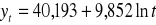
, Współczynnik determinacji =0,936, wariancja resztowa =4,155. Oblicz prognozy produkcji na kolejne trzy kwartały. Czy te prognozy są dopuszczalne, jeśli właściciel dopuszcza błąd nie większy niż 2,5 tys zł.? (
)[źródło:na podstawie Zeliaś A. Prognozowanie ekonomiczne,s.127 zad.3,39]
studia zaoczne 4MSU ćwiczenia 5/6