Ćwiczenie 1.1

a)

nn=(-10:0);

x4=zeros(1,11);

x4(8)=4.5;

stem(nn,x4);

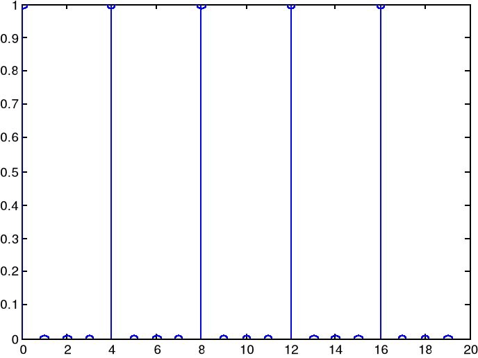
b)

nn=(0:19);

x=[1;0;0;0]*ones(1,5);

x=x(:);

stem(x);

Ćwiczenie 1.2

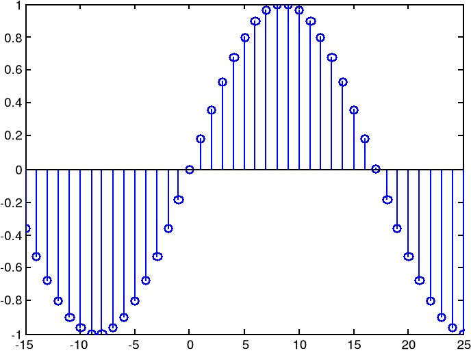
a)

nn=(-15:25);

sinus=sin((pi/17)*nn);

stem(nn,sinus);

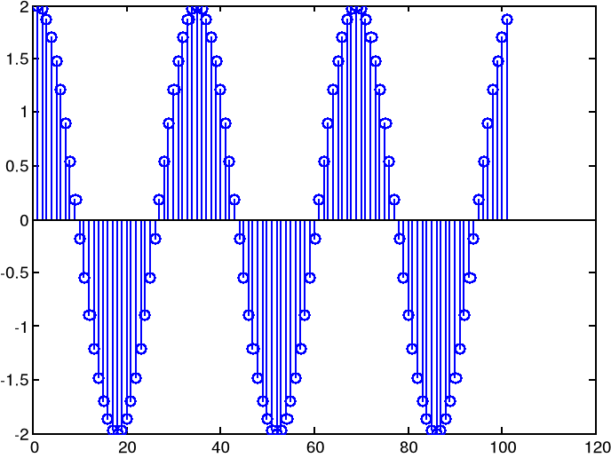
b)

Definicja funkcji

function [x] = moja(amp,omega,faza,pocz,kon)

nn=(pocz:kon);

x=amp*sin(omega*nn+faza);

Wywołanie funkcji dla danych parametrów:

stem(moja(2,pi/17,pi/2,0,100))

Daje wykres:

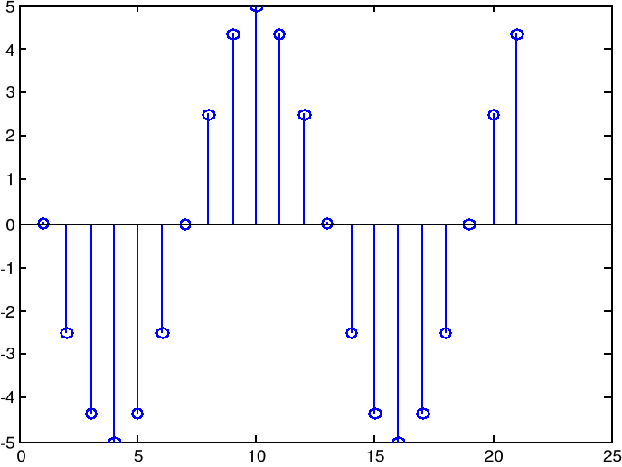
Dla

stem(moja(5,pi/6,pi,0,20))

Uzyskujemy:

Ćwiczenie 1.3

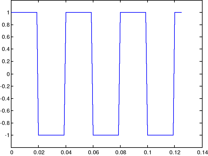
a)

t=0:0.001:0.125;

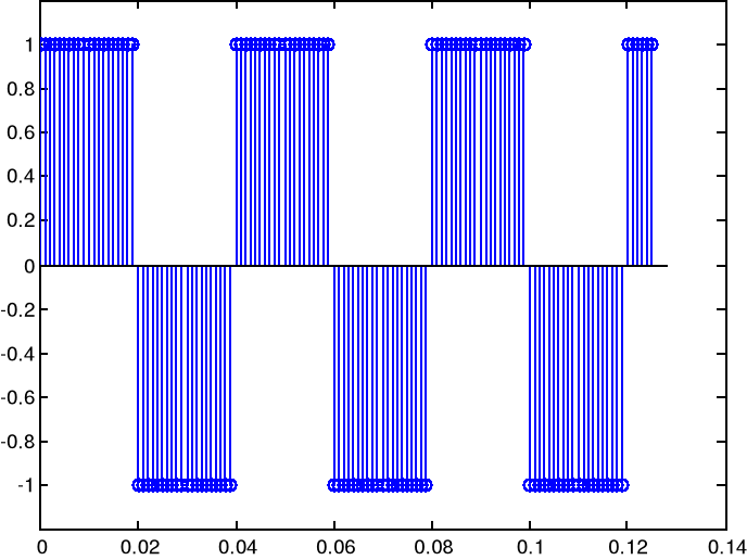
y=square(2*pi*25*t);

efekt instrukcji plot

efekt instrukcji stem(t,y)

b)

T = 4/55;

t = 0:0.01*T:T;

stem(t,5*sawtooth(110*pi*t))

Ćwiczenie 1.4

a)

Zgodnie z instrukcją, funkcja genexp przyjmie postać:

function y=genexp(a,n0,L)

if (L<=0)

error('Dlugosc sygnalu jest nieprawidlowa')

end

nn=n0+[1:L]'-1;

y=a.^nn;

Komenda:

plot(genexp(0.8,0,20))

Komenda:

stem(genexp(0.8,0,20))

b)

Sumowanie wartości sygnału:

for r =1:21

suma = suma + t(r);

end

Wynik:

suma =

4.9424

Z użyciem wzoru:

suma1 = (1-0.8^20)/(1-0.8)

Wynik:

suma1 =

4.9424

c)

Zgodnie z instrukcją:

clear

L=20;

x=zeros(L,1);

x(1)=1;

a=[1 -0.92]

b=[1]

y=filter(b,a,x);

figure(2)

plot(y

Ćwiczenie 2.1.1

a) Zgodnie z instrukcją

t = 0:1/8000:0.01;

f0=300;

x = sin(2*pi*t*f0);

stem(t,x);

c)

subplot(2,2,1)

stem(t,sin(2*pi*t*100))

subplot(2,2,2)

stem(t,sin(2*pi*t*225))

subplot(2,2,3)

stem(t,sin(2*pi*t*350))

subplot(2,2,4)

stem(t,sin(2*pi*t*475))

d)

e)

Analogicznie do c)

Ćwiczenie 2.1.2

a)

b)

subplot(2,1,1)

stem(t,sin(2*pi*t*7525))

subplot(2,1,2)

stem(t,sin(2*pi*t*7650))

subplot(2,1,1)

stem(t,sin(2*pi*t*7775))

subplot(2,1,2)

stem(t,sin(2*pi*t*7900))