POLITECHNIKA SZCZECIŃSKA
KATEDRA MECHANIKI I PODSTAW KONSTRUKCJI MASZYN
Instrukcja do ćwiczeń laboratoryjnych
Numeryczne metody analizy konstrukcji
¼ płyty z otworem
Szczecin 1999Opis zadania
Przykład ten prezentuje zastosowanie p - elementu do zadań płaskiego stanu naprężeń/odkształceń. Jest to stalowa płyta z centralnie umieszczonym otworem Ze względu na symetrię geometrii i obciążeń do obliczeń możemy przyjąć tylko część płyty, z zachowaniem warunków utwierdzenia (na ściance pionowej UX = 0, na ściance poziomej UY = 0). Sprecyzujemy także kryteria zbieżności w punktach krytycznych (maksymalne obciążenia i przemieszczenia).
Kątownik wykonany jest ze stali konstrukcyjnej o module Younga E=2.1·105 MPa i współczynniku Poisona ν=0.27.
■ PREPROCESOR
Nadanie tytułu
(maksymalnie 72 znaki)
Utility Menu: File → Change Title
Wpisz nazwę: Płyta z otworem
OK by zatwierdzić i zamknąć okno
Tytuł będzie wyświetlany w oknie graficznym (ANSYS Graphics) po przerysowaniu okna
Utility Menu: Plot → Replot
Ustawienia preferencji
Okno „Preferences” pozwala wybrać pożądaną dziedzinę analizy (strukturalna, termiczna, mechanika płynów, elektromagnetyczna) oraz jej typ (metoda h, metoda p).
Main Menu: Preferences
1 Włącz analizę strukturalną
2 OK by zatwierdzić i zamknąć okno
Włącz analizę strukturalną
Definiowanie typu elementu i opcji
W każdej dziedzinie analizy należy określić typ elementu (wybrać z biblioteki elementów) stosownie do danej analizy. Każdy element jest określony przez stopnie swobody (przemieszczenia, obroty, temperatury itp.), charakterystyczny kształt (linia, kostka, belka, czworobok itd.), liczby węzłów, oraz to, czy jest rozpatrywany w przestrzeni dwu- czy trójwymiarowej.
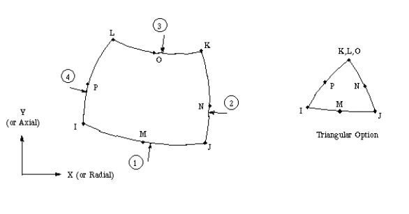
Do obecnej analizy zastosujemy jeden typ elementu, PLANE 145, który jest elementem:
do analizy w przestrzeni 2D,
ośmiowęzłowym,
stopnie swobody: UX, UY.
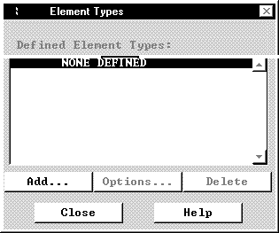
Main Menu: Preprocessor → Element Type → Add/Edit/Delete
1 Dodaj typ elementu
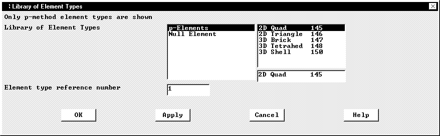
2 Wybierz p - Elements
3 Wybierz element 2D Quad 145 (PLANE 145)
4 OK by zatwierdzić i zamknąć okno
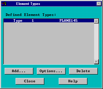
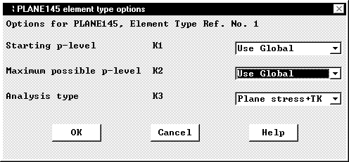
5 Definiowanie opcji elementu PLANE 145
6 Wybierz Plane stress with thickness
7 OK by zatwierdzić i zamknąć okno
8 Close - zamknij
Definiowanie geometrycznych cech elementu
Geometryczne cechy elementu są niezbędne by w pełni opisać budowę danego elementu. Konstrukcja tylko na podstawie węzłów jest niewystarczająca. Typowymi cechami są grubość elementu (thickness), grubość powłoki (dla elementów powłokowych) i właściwości przekroju poprzecznego (dla elementów belkowych).
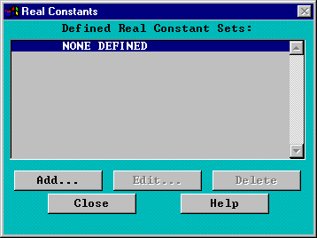
Main Menu: Preprocessor → Real Constants
1 Definiowanie cech
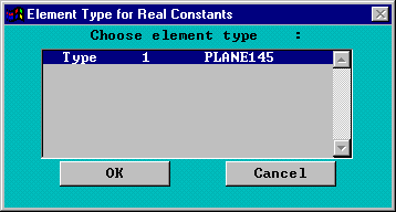
2 OK by wybrać element PLANE 145
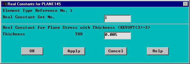
3 Wpisz grubość THK 0.005
4 OK by zatwierdzić i zamknąć okno
5 Zamknij okno definiowania cech
Definiowanie stałych materiałowych
Stałe materiałowe opisują właściwości fizyczne materiału. Zależnie od dziedziny i typu analizy wprowadzane są odpowiednie stałe materiałowe jak:
moduł Younga,
współczynnik Poisona,
współczynnik rozszerzalności cieplnej,
współczynnik przenikania ciepła itp.
Stosownie do aplikacji stałe materiałowe mogą być liniowe, nieliniowe, izo- lub ortotropiczne. Można stworzyć wiele takich zestawów stałych materiałowych odpowiadających różnym materiałom użytym w rozwiązywaniu problemu.
W naszym przypadku w statycznej analizie będzie potrzebny tylko moduł Younga E i współczynnik Poisona ν.
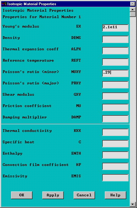
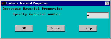
Main Menu: Preprocessor → Material Props → -Constant- Isotropic
1 OK dla zatwierdzenia definiowania materiału 1
2 Wpisz wartość modułu Younga EX = 2.1e11
3 Wpisz wartość współczynnika Poisona NUXY = 0.29
4 OK by zatwierdzić i zamknąć okno
Zapisanie bazy danych
By nie utracić wszystkich nastawów wykonanych dotychczas zapisujemy naszą pracę.
Miejscem docelowym dla pliku powinien być katalog, w którym znajduje się program ANSYS.
Utility Menu: File → Save as... → Save Database to
Wpisz nazwę kplyta z otworem.db i kliknij OK by zatwierdzić i zamknąć okno
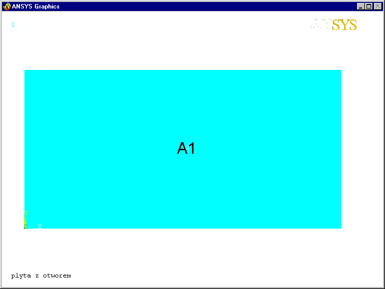
Rysowanie prostokąta
Main Menu: Preprocessor → -Modeling- Create → -Areas- Rectangle →
By 2 Corners
1 Wpisz WP X = 0 (używaj klawisza Tab do przełączania między okienkami)
WP Y = 60
Widht = 0.5
Height = 0.25
OK by stworzyć prostokąt i zamknąć okno
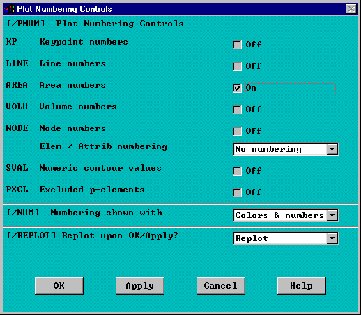
Zmiana ustawień okna graficznego
Uruchomimy opcję numeracji powierzchni. Okno Plot Numbering Controls rozwijane z Utility Menu ukazuje możliwość zastosowania podobnych ustawień dla punktów bazowych, linii, brył, węzłów i elementów.
Utility Menu: Plot Ctrls → Numbering
1 Włącz numerowanie powierzchni
2 OK by zmienić nastawy, zamknąć okno i odświeżyć ekran
Tworzenie okręgu
Utility Menu: Preprocessor → -Modeling- Create → -Areas- Circle → Solid Circle
1 Wpisz WP X = 0, WP Y = 0, Radius = 0.125
2 OK by utworzyć okrąg i zamknąć okno
Zapisanie bazy danych
Utility Menu: File → Save as Jobname.db
Wycinanie ¼ otworu okręgiem
Main Menu: Preprocessor → -Modeling- Operate → -Booleans- Subtract →
Areas
1 Wybierz prostąkąt jako powierzchnię bazową
2 Kliknij Apply
3 Wybierz okrąg do odjęcia
4 OK by odjąć powierzchnie
Zapisanie bazy danych
Utility Menu: File → Save as Jobname.db
Tworzenie siatki elementów skończonych (tryb automatyczny)
Main Menu: Preprocessor → Mesh Tool
1 Wybierz Areas Meshing
Kliknij Mesh
3 Kliknij Pick All
4 Kliknij Close by zamknąć okno
■ SOLVER
Solver jest blokiem, w którym definiuje się obciążenia (siły skupione, momenty, obciążenia ciągłe, temperatury, prędkości płynu itp.), odbiera się stopnie swobody (utwierdzanie) i rozwiązuje się zadanie.
Utwierdzanie płyty
Warunki brzegowe, które zdeklarujemy reprezentują symetryczną naturę problemu. Analiza ¼ modelu odpowiednio utwierdzonego musi prezentować takie same wyniki jak analiza całości.
Utility Menu: PlotCtrls → Numbering
1 Włącz numerowanie linii
2 Wyłącz numerowanie powierzchni
3 OK
Utility Menu: Plot → Areas
Main Menu: Solution → -Loads- Apply → -Structural- Displacement →
On Keypoints
4 Wybierz dwa punkty bazowe definiujące linię 9
5 OK by zakończyć wybieranie
6 Wybierz UY jako zerowe przemieszczenia w kierunku osi Y
7 Wpisz 0 w polu wartości przemieszczenia
Zaznacz rozszerzenie przemieszczenia do węzłów yes (pomiędzy punktami bazowymi)
9 Apply
Zaznaczenie rozszerzenia przemieszczenia do węzłów (KEXPND) pozwala na utwierdzenie nie tylko wybranych 2 punktów bazowych, lecz także wszystkich węzłów zawartych między tymi punktami.
10 Wybierz dwa punkty bazowe definiujące linię 10
11 OK by zakończyć wybieranie
12 Wybierz UX jako zerowe przemieszczenia w kierunku osi X
13 Usuń zaznaczenie utwierdzenia UY
14 OK by zatwierdzić i zamknąć okno
Definiowanie obciążenia
Obciążenie (ciśnienie) będzie przyłożone na linii
Main Menu: Solution → -Loads- Apply → Pressure → On Lines
1 Wybierz linię 2
2 Kliknij OK
3 Wpisz -100 w polu VALI
4 Kliknij OK
Zapisanie bazy danych
Utility Menu: File → Save as Jobname.db
17. Ustalanie kryteriów zbieżności
Main Menu: Solution → - Load Steps Opts - p-Method- Convergence Crit
1 Kliknij Replace
2 Wybierz Local for Solids
3 OK
4 Wybierz węzeł na przecięciu linii 5 i 9
5 OK
6 Zmień procent zbieżności na 1
7 Wybierz DOF solution
8 Wybierz Translation UX
9 OK
10 Kliknij Add
11 OK
12 Wybierz węzeł na przecięciu linii 5 i 10
OK
14 Zmień procent zbieżności na 1
15 Przewiń pasek i wybierz Stress
16 Wybierz X - direction SX
17 OK
Close
Zapisanie bazy danych
Utility Menu: File → Save as Jobname.db
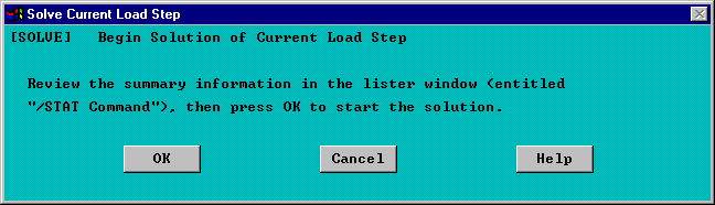
Rozwiązanie problemu
Main Menu: Solution → -Solve- Current LS
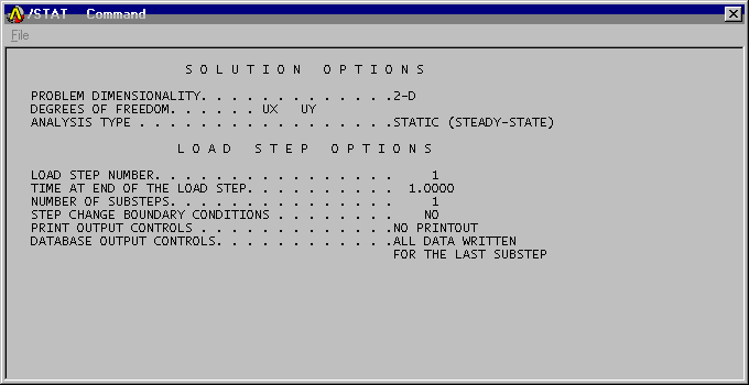
Ogólne informacje o zadaniu dostępne są w oknie statutowym.
By zamknąć okno kliknij File → Close
2 OK by rozpocząć rozwiązywanie
3 Close by zamknąć okno informacyjne po zakończeniu rozwiązywania
■ POSTPROCESOR
W bloku POSTPROCESOR oglądamy rozwiązania naszego zadania. Wyniki są przedstawiane w formie graficznej, w formie tabeli lub z użyciem wykresu.
Wczytanie rezultatów
Main Menu: General Postproc → -Read Results- Lest Set
Kształt płyty
Main Menu: General Postproc → -Plot Results- Deformed Shape...
1 Wybierz kształt odkształcony i nie odkształcony
2 OK by zatwierdzić i zamknąć okno
22. Odczytywanie rezultatów ze wskazaniem miejsca
Utility Menu: PlotCtrls → Device Optrions
1 Włącz Vector mode
2 OK
3 Wybierz Stress
4 Wybierz X-direction SX
5 OK
Klikaj na różnych punktach siatki elementów skończonych by odczytać wartości SX
7 OK
Utility Menu: PlotCtrls → Device Optrions
8 Wyłącz Vector mode
9 OK
23. Rozkład naprężeń w kierunku osi X
Main Menu: General Postproc → Plot Results → -Contour Plot- Nodal Solu
1 Wybierz Stress
2 Wybierz X-direction SX
3 OK
24. Rozkład naprężeń całkowitych
Main Menu: General Postproc → Plot Results → -Contour Plot- Nodal Solu
1 Wybierz Stress
2 Wybierz von Mises SEQV
3 OK
Wyjście z programu ANSYS
Wychodząc z programu można zapisać kształt geometryczny, wszystkie zadane obciążenia i dane rozwiązania zadania.
Utility Menu: File → Exit
1 Wybierz Save Geo + Ld + Solu
OK by wyjść z programu
Laboratorium z ANSYSa 4
2
2
1
14
1
1
2
3
4
3
5
6
7
8
1
2
3
1
3
5
4
1
2
1
2
1
2
1
3
2
2
8
9

7
6
5
1
16
17
18
15
14
11
12
4
3
12
1
3
13
3
3
1
4
4
10
10
6
7
8
9
1
10
1
4
2
7
6
8
3
9
1
2
3
1
2
3
1
4
1
2
3
1
2
2
1
2
4
3
2
Wyszukiwarka