N Feature Neural Network Human Face Recognition

N-Feature Neural Network Human Face Recognition

Javad Haddadnia

, Karim Faez

, Majid Ahmadi

1,3

Electrical and Computer Engineering Department, University of Windsor,

Windsor, Ontario, Canada, N9B 3P4

{javad, ahmadi}@uwindsor.ca

Electrical Engineering Department, Amirkabir University of Technology, Tehran, Iran, 15914

kfaez@cic.aku.ac.ir

Abstract

This paper introduces a novel method for human face
recognition that employs a set of different kind of fea-
tures from the face images with Radial Basis Function
(RBF) neural network called the Hybrid N-Feature
Neural Network (HNFNN) human face recognition
system. The face image is projected in each appropri-
ately selected transform methods in parallel. The output
of the RBF classifiers are fused together to make a deci-
sion. Experimental results for human face recognition
confirm that the proposed method lends itself to higher
classification accuracy relative to existing techniques.

1. Introduction

Face recognition may seem an easy task for humans,

and yet computerized face recognition system still can
not achieve a completely reliable performance. The
difficulties arise due to large variation in facial appear-
ance, head size, orientation and change in environment
conditions. Such difficulties make face recognition one
of the fundamental problems in pattern analysis. In
recent years there has been a growing interest in ma-
chine recognition of faces due to potential commercial
application such as film processing, law enforcement,
person identification, access control systems, etc. A
recent survey of the face recognition systems can be
found in references [1-2].

A complete conventional human face recognition

system should include three stages. The first stage in-
volves detecting the location of face in arbitrary images
[3-4]. The second stage requires extraction of pertinent
features from the localized image obtained in the first
stage. Finally the third stage involves classification of

facial images based on the derived feature vector ob-
tained in the previous stage.

In order to design a high accuracy recognition sys-

tem, the choice of feature extractor is very crucial. Two
main approaches to feature extraction have been exten-
sively used in conventional techniques [2]. The first one
is based on extracting structural facial features that are
local structure of face images, for example, the shapes
of the eyes, nose and mouth. The structure-based ap-
proaches deal with local information instead of global
information. Therefor they are not affected by irrelevant
information in an image. It has been shown that the
structure-based approaches by explicit modeling of
facial features have been troubled by the unpredictabil-
ity of face appearance and environmental condition [2].
The second one is based on statistical approaches when
features are extracted from the whole image and there-
fore use global information instead of local information.
Since the global data of an image are used to determine
the feature elements, data that are irrelevant to facial
portion such as hair, shoulders and background may
contribute to creation of erroneous feature vectors that
can affect the recognition results [5].

In the field of pattern recognition, the combination of

an ensemble of classifiers has been proposed to achieve
image classification systems with higher performance in
comparison with the best performance achievable em-
ploying a single classifier. This has been verified ex-
perimentally in the literature [6-7]. A number of image
classification systems based on the combination of out-
puts of different classifier systems have been proposed.
Different structures for combining classifier systems can
be grouped in three configurations [8-9]. In the first
group, the classifier systems are connected in cascade to
create pipeline structure. In the second one, the classi-
fier systems are used in parallel and their outputs are
combined named it parallel structure. Finally the hybrid
structure is a combination of the pipeline and parallel

structures. In this paper, we propose a human face rec-
ognition system that can be designed based on hybrid
structure classifier system to have evolutionary recogni-
tion results by developing the N-features and selecting
them for the recognition problem. This human face
recognition system uses available information and ex-
tracts more characteristics for face classification pur-
pose by extracting different feature domains from input
images. In this paper three different feature domains
have been used for extracting features from input im-
ages. These include Pseudo Zernike Moment Invariant
(PZMI) and Zernike Moment Invariant (ZMI) which
produce the best result for human face recognition in
comparison with other moments [10] and also Principal
Component Analysis (PCA) [11].

Finally in this paper Radial Basis Function (RBF)

neural network is used as the classifier. Recently RBF
neural networks have found to be very attractive for
many engineering problems. An important property of
RBF neural networks is that they form a unifying link
among many different research fields such as function
approximation, regularization, noisy interpolation and
pattern recognition. The increasing popularity of RBF
neural networks is partly due to their simple topological
structure, their locally tuned neurons and their ability to
have a fast learning algorithm in comparison with the
multi-layer feed forward neural networks [10][12]. The
rest of this paper is organized as follows. The proposed
human face recognition system is developed in section
2. Section 3 presents the feature domains. The classifi-
cation technique is described in section 4. Finally sec-
tion 5 and 6 presents the experimental results and con-
clusion.

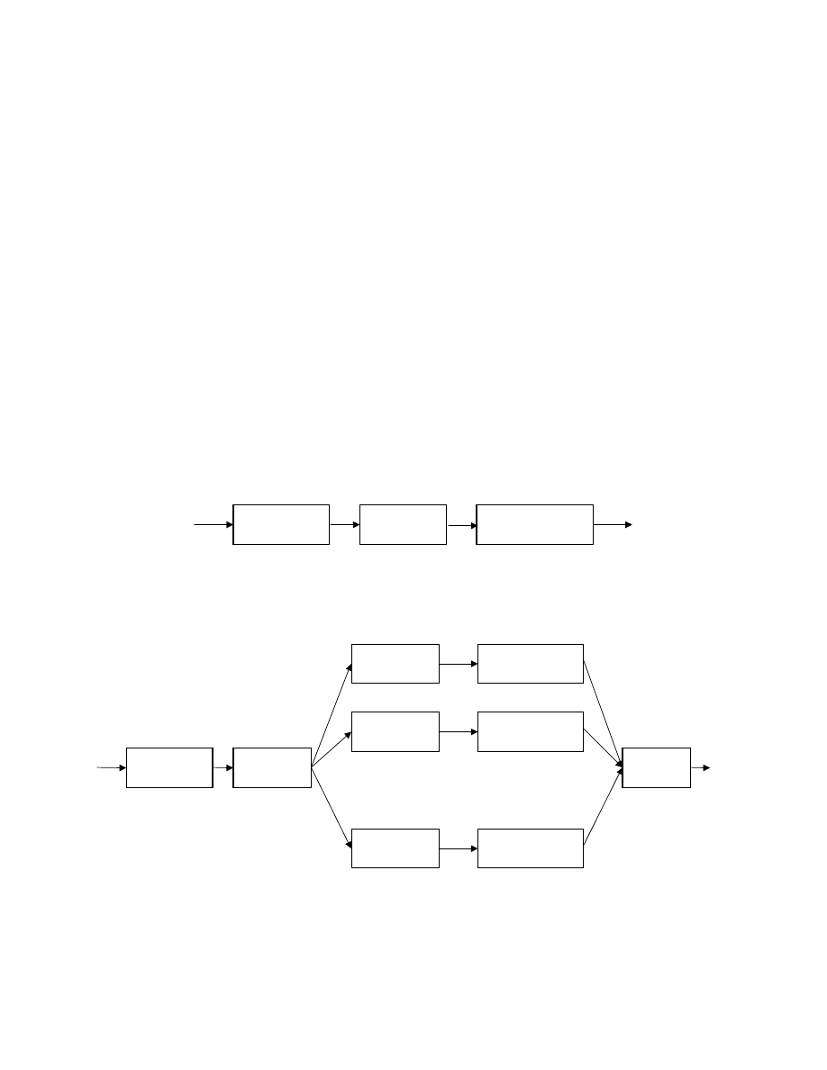
2. The Proposed HNFNN

Fig. (1) shows a conventional human face recogni-

tion. This system uses one feature domain and one clas-
sifier. Usually neural network are used as classifier
therefore this conventional method named Single Fea-
ture Neural Network (SFNN) human face recognition
system. The Proposed human face recognition has been
shown in Fig. (2). Unlike conventional human face
recognition system the proposed HNFNN system is
developed in five stages. In the first step, face localiza-
tion process is done. To ensure a robust, accurate feature
extraction that distinguishes between face and nonface
region in an image, we require the exact location of the
face region. In this paper we have used a modified ver-
sion of shape information technique that presented in
reference [3] for face localization. After face localiza-
tion, in the second stage we have created a subimage,
which contains information needed for recognition algo-
rithm. By using a subimage, data that are irrelevant to
facial portion are disregarded. In the third stage, differ-

ent features are extracted in parallel from the derived
subimage. These features are obtained from the different
domains. The fourth stage required classification, which
classify a new face image, based on the chosen features,
into one of the possibilities. This is done for each fea-
ture domain in parallel as Fig. (2) shows. Finally the last
stage combines the outputs of each neural network clas-
sifiers to construct the identification. In this paper ma-
jority method has been selected for decision strategy.

2.1. Face Localization

Many algorithms have been proposed for face local-

ization and detection. A critical survey on face localiza-
tion and detection can be found in reference [2]. The
ultimate goal of the face localization is finding an object
in an image as a face candidate that its shape resembles
the shape of a face. Faces are characterized by elliptical
shape and an ellipse can approximate the shape of a
face. A technique is presented in [3], which finds the
best-fit ellipse to enclose the facial region of the human
face in a frontal view of facial image. In this algorithm
an ellipse model with five parameters has been used.
Initially connected component objects are determined
by applying a region-growing algorithm. Consequently
for each connected component object with a given
minimum size, the best-fit ellipse is computed on the
basis of its moments. To assess how well the connected
component object is approximated by its best-fit ellipse,
we define the new distances measure between the con-
nected component object and the best-fit ellipse as fol-
lows:

inside

outside

where the

inside

is the number of background points

inside the ellipse,

outside

is the number of points of the

connected component object that are outside of the
ellipse and

is the size of the connected component

object [3]. The connected component object is closely
approximated by its ellipse when

and

is as small

as possible. We have named the threshold values for
both

and

as Facial Candidate Threshold (FCT).

Our experimental study indicates that when FCT is less
than 0.1 the connected component is very similar to
ellipse therefore it is a good candidate as a face region.
If

and

are grater than FCT, there is no face re-

gion in the input image therefor we reject it as nonface
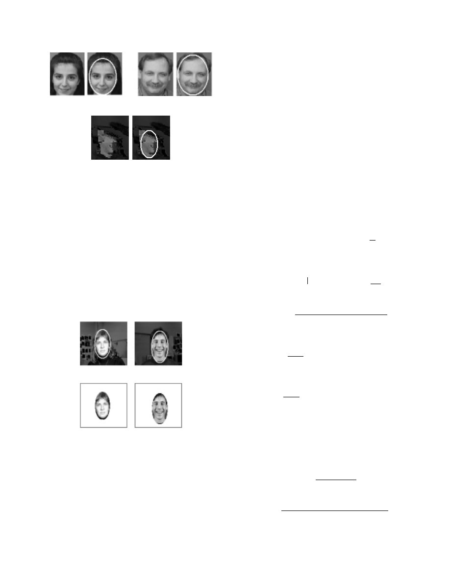
image [13]. An example of applying this method for
locating a face candidate and rejecting nonface image
has been shown in Fig. (3). Subsequently the rest of the
system processes the selected face candidates for recog-
nizing.

065

008

062

011

191

Figure 3: Distinguishing between face and nonface

using best-fit ellipse and FCT threshold

2.2. Subimage Formation

The subimage encloses the pertinent information

around the face in an ellipse that was explained in sec-
tion 2.1 while pixel value outside the ellipse is set to
zero. Fig. (4) shows sample of selecting of face location
and creating of subimage in feature extracting respec-
tively. By using subimage, data that are irrelevant to
facial portion such as hair, shoulders and background
are disregarded and the speed of computing various
features is increased due to smaller pixels content of the
subimages.

(a) Face location

(b) subimage

Figure 4: Creating subimages from face images

3. N-Features Domains

In order to design a good face recognition system, the

choice of feature extractor is very crucial. To design a
system with low to moderate complexity the feature
vectors should contain the most pertinent information
about the face to be recognized. Face recognition system

should be capable of recognizing unpredictability of
face appearance and changing environment. In the pro-
posed system, N different feature domains are extracted
from the derived subimages in parallel. Therefore this
approach can extract more characteristics of face images
for classification purpose. In this paper we set N=3 and
therefore three different kind of feature domains have
been selected. These include PZMI, ZMI and PCA.

3.1. Pseudo Zernike Moment Invariant

The advantages of considering orthogonal moments

are that they are shift, rotation and scale invariant and
very robust in the presence of noise. We have used the
PZMI for generating feature vector elements. Pseudo
Zernike polynomials are well known and widely used in
the analysis of optical systems. Pseudo Zernike poly-
nomials are orthogonal set of complex-valued polyno-
mials defined as [10][14]:

))

(

tan

exp(

)

(

)

(

−

where

≤

≥

≤

is even and Radial

polynomials

are defined as:

)

(

)

(

−

∑

(

)

(

−

The PZMI of order n and repetition m, can be com-

puted as follows:

( )( )

m
b

k
a

even

)

(

PZMI

∑∑

∑

= =

−

)

(

−

( )( )

m
b

d
a

odd

)

(

∑∑

∑

−

)

(

−

where

)

(

−

)

(

−

is the

scale invariant central moments and

is the scale

invariant radial geometric moments are defined as:

)

(
00

)

(
00

)

)(

(

∑ ∑

)

where

−

)

−

)

and

x ,

y are defined as follow:

)

(

∑ ∑

)

(

)

(

)

(

−

∑ ∑

3.2. Zernike Moment Invariant

Zernike polynomials are orthogonal set of complex-

valued polynomials defined as:

))

(

tan

exp(

)

(

)

(

−

where

≤

≥

≤

and

−

is even

and Radial polynomials {

} are defined as:

(

)

(

)

(

−

∑

where:

(

)

(

−

The complex Zernike moments [19] of order n and

repetition m are given by:

)

(

)

(

ZMI

∑ ∑

To utilize the shift invariant property of moments, we

have used ZMI from the scale invariant central moments

(

) as follows [14]:

( )( )

∑∑

∑

−

b
a

(

ZMI

)

(

−

where

(

−

3.3. Principal Component Analysis

PCA is a well-known statistical technique for feature

extraction. Each

image in the training set was

row concatenated to form

vectors

. Given a

set of

training images

,...

}

{

the mean

vector of the training set was obtained as:

∑

The average vector was subtracted out from the

training vectors to obtain:

−

, i=1,2,3,…

matrix A was constructed with the

T
i

as its row vectors. The singular value decomposi-

tion of A can then be written as:

where

is an

diagonal matrix with singular

values

arranged in descending order, and V and

U are

and

orthogonal matrices,

respectively. V is composed of the eigenvectors of

, while U is composed of the eigenvectors of

. These are related by:

where

ˆ consists of the eigenvectors of

, which

correspond to the non-zero singular values. This relation
allows a smaller

eigenvalue problem for

to be solved, and to subsequently obtain

ˆ by

matrix multiplication.

The projection of a face vector onto the space of

N eigenfaces results in an

N -dimensional feature

vector of projection weights. As PCA has the property
of packing the greatest energy into the least number of
principal components, the smaller principal components
which are less than a threshold can be discarded with
minimal loss in representational capability. This dimen-
sionality reduction results in face weight vectors of

dimensions

. An appropriate value of

can be chosen by considering the Basis Restriction

Error (BRE) as a function of

[11]. This gradual

decrease in error is significant for recognition tech-
niques based on eigenfaces where storage and computa-

tional performance are directly related to

N .

4. Classifier Design

Neural networks have been employed and compared

to conventional classifiers for a number of classification
problems. The results have shown that the accuracy of
the neural network approaches equivalent to, or slightly
better than, other methods. Also, due to the simplicity,
generality and good learning ability of the neural net-
works, these types of classifiers are found to be more
efficient [10][12]. Radial Basis Function (RBF) neural

networks have found to be very attractive for many
engineering problem because: (1) they are universal
approximators, (2) they have a very compact topology
and (3) their learning speed is very fast because of their
locally tuned neurons. Therefore the RBF neural net-
works serve as an excellent candidate for pattern appli-
cations and attempts have been carried out to make the
learning process in this type of classification faster than
normally required for the multi-layer feed forward neu-
ral networks [12].

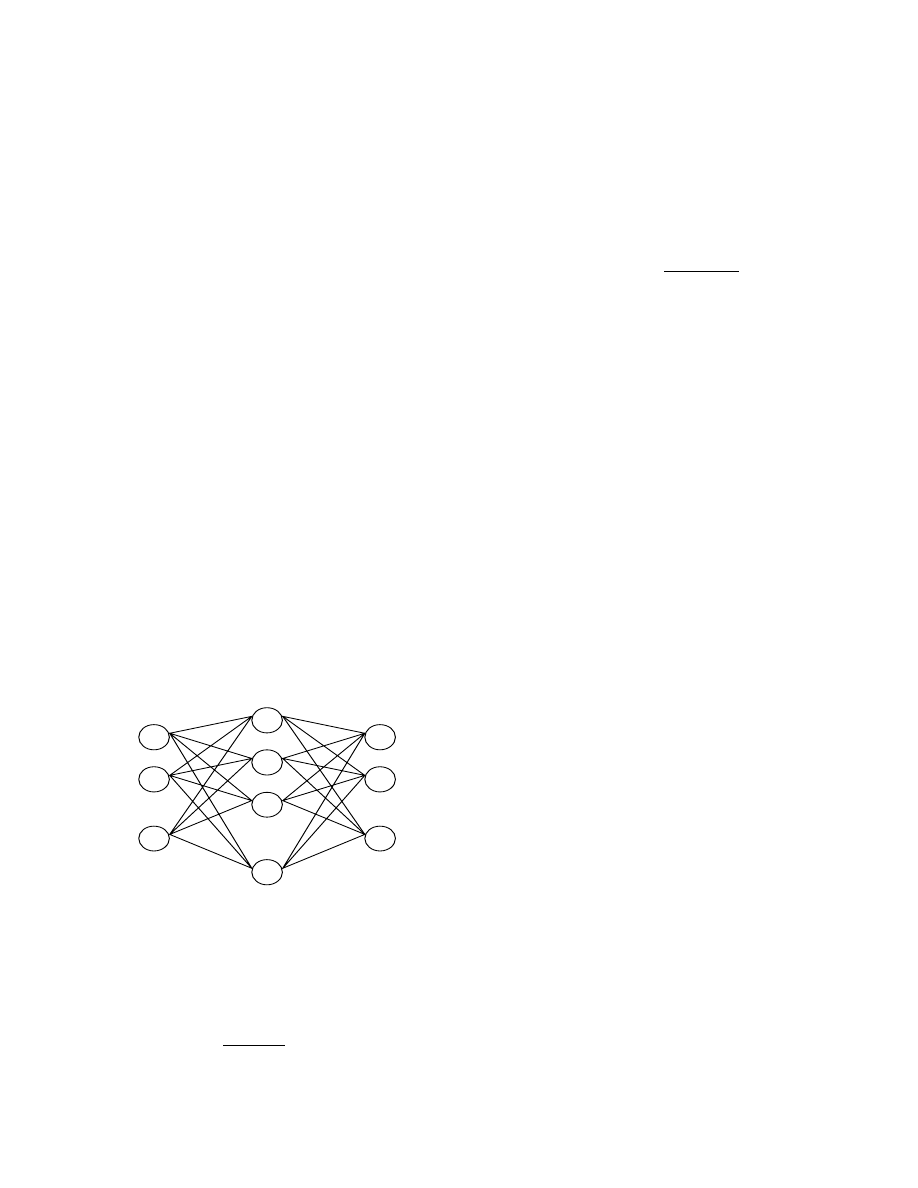
4.1. RBF Neural Network Structure

An RBF neural network structure is shown in Fig.

(5), which has architecture similar to that of a traditional
three-layer feed forward neural network. The construc-
tion of the RBF neural network involves three different
layers with feed forward architecture. The input layer of
this network is a set of n units, which accept the ele-
ments of an n-dimensional input feature vector. The
input units are fully connected to the hidden layer with r
hidden units. Connections between the input and hidden
layers have unit weights and, as a result, do not have to
be trained. The goal of the hidden layer is to cluster the
data and reduce its dimensionality. In this structure
hidden layer is named RBF units. The RBF units are
also fully connected to the output layer. The output
layer supplies the response of neural network to the
activation pattern applied to the input layer. The trans-
formation from the input space to the RBF-unit space is
nonlinear, whereas the transformation from the RBF-
unit space to the output space is linear.

1 1

r s

Figure 5: RBF neural network structure

The RBF neural network is a class of neural net-

works, where the activation function of the hidden units
is determined by the distance between the input vector
and a prototype vector. The activation function of the
RBF units is expressed as follow [10][12]:

)

(

)

(

−

i=1,2,…,r

It should be noted that x is an n-dimensional input

feature vector,

c is an n-dimensional vector called the

center of the RBF unit,

is the width of RBF unit and

r is the number of the RBF units. Typically the activa-
tion function of the RBF units is chosen as a Gaussian
function with mean vector

and variance vector

as follows:

)

exp(

)

(

2
i

−

Note that

2
i

represents the diagonal entiries of co-

variance matrix of Gaussian function. The output units
are linear and therefore the response of the j-th output
unit for input x is given as:

∑

)

(

)

(

)

(

)

(

where

)

(

is the connection weight of the i-th RBF

unit to the j-th output node and

)

(

is the bias of the j-

th output. The bias is omitted in this network in order to
reduce network complexity. Therefore:

∑

)

(

)

(

)

(

4.2. RBF Based Classifier Design

RBF neural network classifier can be viewed as a

function mapping interplant that tries to construct hy-
persurfaces, one for each class, by taking a linear com-
bination of the RBF units. These hypersurfaces can be
viewed as discriminant functions, where the surface has
a high value for the class it represents and a low value
for all others. An unknown input feature vector is classi-
fied as belonging to class associated with the hypersur-
face with the largest output at that point. In this case the
RBF units’ serve as components in a finite expansion of
the desired hypersurface where the component coeffi-
cients (the weights) have to be trained [12][15].

For designing a classifier based on RBF neural net-

work, we have set the number of input nodes in the
input layer of neural network equal to the number of
feature vector elements. The number of nodes in the
output layer is set to the number of image classes. The
RBF units are selected using the following clustering
procedure [15]:
Step1

: Initially the RBF units are set equal to the num-

ber of outputs.

Step2

: For each class k, the center of RBF units (

) is

selected as the mean value of the sample patterns
belonging to the same class, i.e.

i
k

∑

, k=1,2,…,s

where

i
k

x is the i-th sample pattern belonging to

class k and

N is the number of samples pattern

in the same class.

Step3: For each class k, compute the distance

f
k

d from

the mean

to the farthest sample pattern

f
k

in that class:

f
k

−

, k=1,2,…,s

Step4:

For each class k, compute the distance

)

(

between the mean of the class and the mean of
other classes and then find the minimum among
the distances computed:

)

(

−

))

(

min(

)

(

min

where j=1,2,…,s and

≠

. Then we check the

relationship between

)

(

min

f
k

, and

f
l

. If

)

(

min

f
l

f
k

≤

then class k is not over-

lapping with other classes. Otherwise, class k is
overlapping with other classes and misclassifica-
tions may occur in this case.

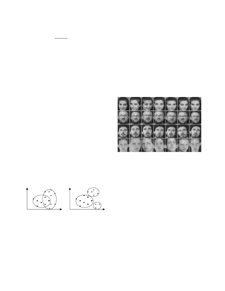
Step5: If two classes are overlapped strongly, we first

split one of the classes into two to remove the
overlap. If the overlap is not removed the second
class is also split. This requires addition of a new
RBF unit to the hidden layer. This can be seen in
Fig. (5).

Step6: Repeat steps 2 to 5 until all the training sample

patterns are clustered correctly in the hidden
layer.

Figure 6: One class split into two classes

The above procedure determines the number of RBF

units, r, in the RBF neural network structure. In addi-
tion, we select the mean values of all the clusters, which
have been determined by the above procedure as the
initial center of the RBF units.

Training of the RBF neural network involves esti-

mating output connection weights, centers and widths of
the RBF units. We use the HLA method, which com-
bines the gradient method and the linear least squared
method for training RBF neural network [15].

5. Experimental Results

To check the utility of our proposed algorithm ex-

perimental studies are carried out on the ORL database
images of Cambridge University. 400 face images from
40 individuals in different states from the ORL database
have been used to evaluate the performance of the pro-
posed method. None of the 10 samples are identical to
each other. They vary in position, rotation, scale and
expression. In this database each person has changed his
face expression in each of 10 samples (open/close eye,
smiling/not smiling). For some individuals, the images
were taken at different times, varying facial details
(glasses/no glasses). Samples of database used are
shown in Fig. (7).

Figure 7: Sample of face database

A sample of the proposed system with three different

feature domains and the RBF neural network has been
developed. In this example, for the PZMI and ZMI all
moments from order 9 to 10 have been considered as
feature vector elements. The feature vectors for these
domains have 21 elements for the PZMI and 11 ele-
ments for the ZMI. Also for the PCA feature vector has
been created based on the 30 largest PCA number for
each image. A total of 200 images have been used to
train and another 200 for test. Each training set consists
of 5 randomly chosen images from the same class in the
training stage. In the face localization step, shape infor-
mation algorithm with FCT=0.1 has been applied to all
images. Subsequently, subimage has been created from
the derived localized face image. Recognition rate of
99.7% was obtained using this proposed technique.

To compare the effectiveness of the proposed method

in comparison with the SFNN human face recognition
systems, we have developed the SFNN systems using
the PZMI+RBF [10], ZMI+RBF [10] and PCA+RBF.
For these systems we have selected the PZMI as feature
domain with order 9 and 10 which has 21 elements,
ZMI with order 9 and 10 with 11 feature elements and
finally PCA with 30 largest value. The comparison of

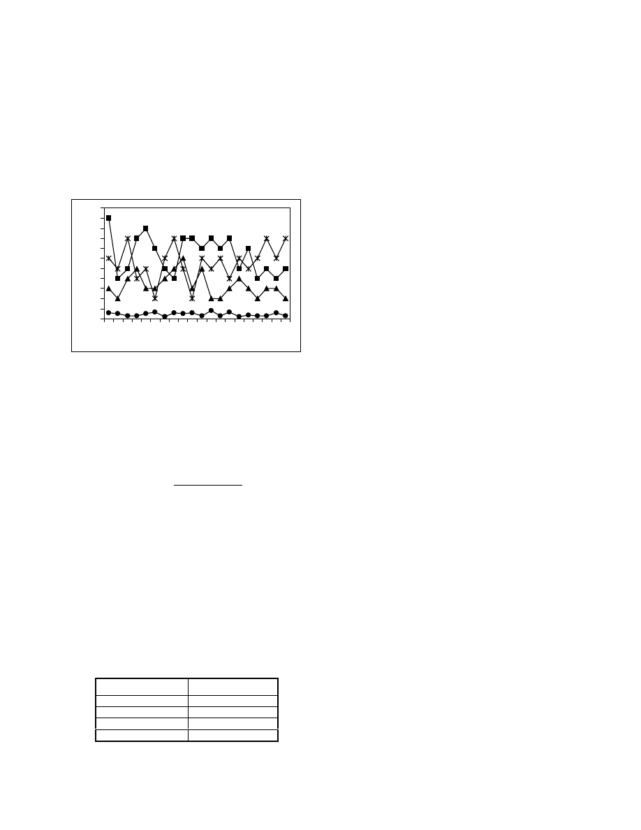
the HNFNN with each individual classifiers as a func-
tion of class number has been shown in Fig. (8). From
the results, these can be no doubt that the recognition
rate of the HNFNN is much better than that of any indi-
vidual classifiers. From this figure it is clear that the
output of each individual classifier may agree or conflict
with each other but the HNFNN search for a maximum
degree of agreement between the conflicting supports of
a face pattern.

Class Numbers

rate(

PZMI

PCA

ZMI

HNFNN

Figure 8: Error rate in the HNFNN and each individual

classifier based on class number

Also to demonstrate the effectiveness of the human

face recognition system by the proposed method, we
have compared the proposed method with other algo-
rithms. To make this comparison meaningful, an aver-
age overall error rate is defined as:

ave

)

(

∑

where m is the number of experimental runs, each being
performed on random partition of the database into sets,

)

(

is the number of misclassification for the i-th

run, and

is the number of total testing images for

each runs. In our study the ORL database was used in
the experiments and methods reported in [10], [16] and
[17] were used for comparison purpose. Table (1) shows
the results of this comparative study. In this table the
SFNN denotes the Shape Information with Neural Net-
work that was reported in [10], CNN is the Convolution
Neural Network method used in [16] and also NFL for
Nearest Feature Line method in [17].

Table 1: Error rate in different methods

Methods

ave

CNN [16]

3.83

NFL [17]

3.125

SFNN [10]

1.323

Proposed method

0.283

6. Conclusion

This paper presented a novel method for the recogni-

tion of human faces in 2-Dimensional digital images.
The proposed technique is based on the Hybrid N-
Feature Neural Network (HNFNN) structure. An im-
plementation example is given to demonstrate the feasi-
bility of the HNFNN human face recognition system. It
employs the RBF neural networks and three feature
domains. These include PZMI, ZMI and PCA. The
highest recognition rate of 99.7% with the ORL data-
base was obtained using this proposed algorithm. Com-
parison with some of the existing traditional technique
in the literatures on the same database indicates the
usefulness of the proposed technique.

References

[1]

M. A. Grudin, “On Internal Representation in face Rec-
ognition Systems”, Pattern. Recognition. Vol. 33, No. 7,
pp.1161-1177, 2000.

[2]

J. Daugman, “Face Detection: A Survey”, Computer
Vision and Image Understanding, Vol. 83, No. 3, pp.
236-274, Sept. 2001.

[3]

J. Haddadnia, K. faez, “Human Face Recognition Based
on Shape Information and Pseudo Zernike Moment”, 5

Int. Fall Workshop Vision, Modeling and Visualization,
Saarbrucken, pp. 113-118, Germany, Nov. 22-24, 2000.

[4]

J. Wang and T. Tan, “A New Face Detection Method
Based on Shape Information”, Pattern Recognition Let-
ter, Vol. 21, pp. 463-471, 2000.

[5]

L. F. Chen, H. M. Liao, J. Lin and C. Han, “Why Recog-
nition in a statistic-based Face Recognition System
should be based on the pure Face Portion: A Probabilistic
decision-based Proof”, Pattern Recognition, Vol. 34, No.
7, pp. 1393-1403, 2001.

[6]

G. Giacinto, F. Roli and G. Fumera, “Unsupervised
Learning of Neyral Network Ensembles for Image Classi-
fication”, IEEE Int. Joint Conf. On Neural Network, Vol.
3, pp. 155-159, 2000.

[7]

J. Kittler, M. Hatef, R. P. W. Duin and J. Matas, “On
Combining Classifier”, IEEE Trans. On Patt. Anal. and
Mach. Intel., Vol. 20, pp. 226-239, March 1998.

[8]

T. K. Ho, J. J. Hull and S. N. Srihari, “Decision Combi-
nation in Multiple Classifier Systems”, IEEE Trans. On
Patt. Anal. and Mach. Intel., Vol. 16, No. 1, pp. 66-75,
Jan. 1994.

[9]

Y. Lu, “Knowledge Integrations in a Multiple Classifier
System”, Applied Intelligence, Vol. 6, No. 2, pp. 75-86,
April 1996.

[10]

J. Haddadnia, K. Faez, P. Moallem, “Neural Network
Based Face Recognition with Moments Invariant”, IEEE
Int. Conf. On Image Processing, Vol. I, pp. 1018-1021,
Thessaloniki, Greece, 7-10 October 2001.

[11]

M. Truk and A. Pentland, “Eigenfaces for Recognition”,
Journal Cognitive Neuroscience, Vol. 3, No. 1, pp. 71-
86, 1991.

[12]

W. Zhou, “Verification of the nonparametric character-
istics of backporpagation neural networks for image
classi

[13]

fication”, IEEE Trans. On Geo. and Remote Sensing,
Vol. 37, No. 2, pp. 771-779, March 1999.

[14]

J. Haddadnia, M. Ahmadi, K. Faez, “An Efficient
Method for Recognition of Human Face Recognition
Using Higher Order Pseudo Zernike Moment Invariant”,
The 5

IEEE Int. Conf. on Automatic Face and Gesture

Recognition, Washington, DC, USA, May 20-21, 2002,
Accepted for presentation.

[15]

C. H. The and R. T. Chin, “On Image Analysis by the
Methods of Moments”, IEEE Trans. On Patt. Anal. and
Mach. Intel., Vol. 10, No. 4, pp. 496-513, 1988.

[16]

J. Haddadnia, M. Ahmadi, K. Faez, “A Hybrid Learning
RBF Neural Network for Human Face Recognition with
Pseudo Zernike Moment Invariant”, IEEE Int. Joint
conf. on Neural Network, Honolulu, HI, May 12-17,
2002, Accepted for presentation.

[17]

S. Lawrence, C. L. Giles, A. C. Tsoi and A. D. Back,
“Face Recognition: A Convolutional Neural Networks
Approach”, IEEE Trans. on Neural Networks, Special
Issue on Neural Networks and Pattern Recognition, Vol.
8, No. 1, pp. 98-113, 1997.

[18]

S. Z. Li and J. Lu, “Face Recognition Using the Nearest
Feature Line Method”, IEEE Trans. on Neural Net-
works, Vol. 10, pp. 439-443, 1999.

Input image

Output person

Figure 1: SFNN human face recognition system

Figure 2: HNFNN based human face recognition system

Face

Localization

Feature

Extraction

Neural Network

Classifier

Feature

Extractor 1

Neural Network

Classifier 1

Feature

Extractor 2

Feature

Extractor N

Neural Network

Classifier 2

Neural Network

Classifier N

Decision

Strategy

Face

Localization

Subimage

Creation

Wyszukiwarka

Podobne podstrony:
Neural networks in non Euclidean metric spaces
Artificial Neural Networks for Beginners
A neural network based space vector PWM controller for a three level voltage fed inverter induction
Artificial neural network based kinematics Jacobian
Neural Network I SCILAB id 3172 Nieznany
Prediction Of High Weight Polymers Glass Transition Temperature Using Rbf Neural Networks Qsar Qspr
Artificial Neural Networks The Tutorial With MATLAB
Neural Network II SCILAB id 317 Nieznany
An Artificial Neural Networks Primer with Financial
Neural networks in non Euclidean metric spaces
Artificial Neural Networks for Beginners
Geoffrey Hinton, Ruslan Salakhutdinov Reducing the dimensionality of data with neural networks
Fast virus detection by using high speed time delay neural networks
Adrian Silvescu Fourier Neural Networks (Article)

więcej podobnych podstron