The setup for measuring the SHG is described

in the supporting online material (22). We expect
that the SHG strongly depends on the resonance
that is excited. Obviously, the incident polariza-
tion and the detuning of the laser wavelength
from the resonance are of particular interest. One
possibility for controlling the detuning is to
change the laser wavelength for a given sample,
which is difficult because of the extremely broad
tuning range required. Thus, we follow an
alternative route, lithographic tuning (in which
the incident laser wavelength of 1.5 mm, as well
as the detection system, remains fixed), and tune
the resonance positions by changing the SRR
size. In this manner, we can also guarantee that
the optical properties of the SRR constituent
materials are identical for all configurations. The
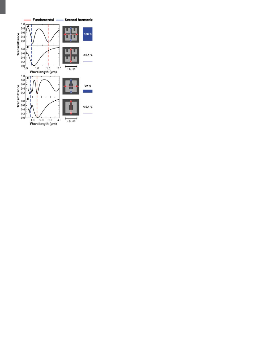
blue bars in Fig. 1 summarize the measured SHG
signals. For excitation of the LC resonance in Fig.
1A (horizontal incident polarization), we find
an SHG signal that is 500 times above the noise
level. As expected for SHG, this signal closely
scales with the square of the incident power
(Fig. 2A). The polarization of the SHG emission
is nearly vertical (Fig. 2B). The small angle with
respect to the vertical is due to deviations from
perfect mirror symmetry of the SRRs (see
electron micrographs in Fig. 1). Small detuning
of the LC resonance toward smaller wavelength
(i.e., to 1.3-mm wavelength) reduces the SHG
signal strength from 100% to 20%. For ex-
citation of the Mie resonance with vertical
incident polarization in Fig. 1D, we find a small
signal just above the noise level. For excitation
of the Mie resonance with horizontal incident
polarization in Fig. 1C, a small but significant
SHG emission is found, which is again po-

larized nearly vertically. For completeness, Fig.
1B shows the off-resonant case for the smaller
SRRs for vertical incident polarization.

Although these results are compatible with

the known selection rules of surface SHG from
usual nonlinear optics (23), these selection rules
do not explain the mechanism of SHG. Follow-
ing our above argumentation on the magnetic
component of the Lorentz force, we numerically
calculate first the linear electric and magnet-
ic field distributions (22); from these fields,
we compute the electron velocities and the
Lorentz-force field (fig. S1). In the spirit of a
metamaterial, the transverse component of the
Lorentz-force field can be spatially averaged
over the volume of the unit cell of size a by a
by t. This procedure delivers the driving force
for the transverse SHG polarization. As usual,
the SHG intensity is proportional to the square
modulus of the nonlinear electron displacement.
Thus, the SHG strength is expected to be
proportional to the square modulus of the
driving force, and the SHG polarization is
directed along the driving-force vector. Cor-
responding results are summarized in Fig. 3 in
the same arrangement as Fig. 1 to allow for a
direct comparison between experiment and
theory. The agreement is generally good, both
for linear optics and for SHG. In particular, we
find a much larger SHG signal for excitation of
those two resonances (Fig. 3, A and C), which
are related to a finite magnetic-dipole moment
(perpendicular to the SRR plane) as compared
with the purely electric Mie resonance (Figs.
1D and 3D), despite the fact that its oscillator
strength in the linear spectrum is comparable.
The SHG polarization in the theory is strictly
vertical for all resonances. Quantitative devia-
tions between the SHG signal strengths of ex-
periment and theory, respectively, are probably
due to the simplified SRR shape assumed in
our calculations and/or due to the simplicity of
our modeling. A systematic microscopic theory
of the nonlinear optical properties of metallic

metamaterials would be highly desirable but is
currently not available.

References and Notes

1. J. B. Pendry, A. J. Holden, D. J. Robbins, W. J. Stewart,

IEEE Trans. Microw. Theory Tech. 47, 2075 (1999).

2. J. B. Pendry, Phys. Rev. Lett. 85, 3966 (2000).
3. R. A. Shelby, D. R. Smith, S. Schultz, Science 292, 77 (2001).
4. T. J. Yen et al., Science 303, 1494 (2004).
5. S. Linden et al., Science 306, 1351 (2004).
6. C. Enkrich et al., Phys. Rev. Lett. 95, 203901 (2005).
7. A. N. Grigorenko et al., Nature 438, 335 (2005).
8. G. Dolling, M. Wegener, S. Linden, C. Hormann, Opt.

Express 14, 1842 (2006).

9. G. Dolling, C. Enkrich, M. Wegener, C. M. Soukoulis,

S. Linden, Science 312, 892 (2006).

10. J. B. Pendry, D. Schurig, D. R. Smith, Science 312, 1780;

published online 25 May 2006.

11. U. Leonhardt, Science 312, 1777 (2006); published

online 25 May 2006.

12. M. W. Klein, C. Enkrich, M. Wegener, C. M. Soukoulis,

S. Linden, Opt. Lett. 31, 1259 (2006).

13. W. J. Padilla, A. J. Taylor, C. Highstrete, M. Lee, R. D. Averitt,

Phys. Rev. Lett. 96, 107401 (2006).

14. D. R. Smith, S. Schultz, P. Markos, C. M. Soukoulis, Phys.

Rev. B 65, 195104 (2002).

15. S. O’Brien, D. McPeake, S. A. Ramakrishna, J. B. Pendry,

Phys. Rev. B 69, 241101 (2004).

16. J. Zhou et al., Phys. Rev. Lett. 95, 223902 (2005).
17. A. K. Popov, V. M. Shalaev, available at http://arxiv.org/

abs/physics/0601055 (2006).

18. V. G. Veselago, Sov. Phys. Usp. 10, 509 (1968).
19. M. Wegener, Extreme Nonlinear Optics (Springer, Berlin,

2004).

20. H. M. Barlow, Nature 173, 41 (1954).
21. S.-Y. Chen, M. Maksimchuk, D. Umstadter, Nature 396,

653 (1998).

22. Materials and Methods are available as supporting

material on Science Online.

23. P. Guyot-Sionnest, W. Chen, Y. R. Shen, Phys. Rev. B 33,

8254 (1986).

24. We thank the groups of S. W. Koch, J. V. Moloney, and

C. M. Soukoulis for discussions. The research of
M.W. is supported by the Leibniz award 2000 of the
Deutsche Forschungsgemeinschaft (DFG), that of S.L. through
a Helmholtz-Hochschul-Nachwuchsgruppe (VH-NG-232).

Supporting Online Material

www.sciencemag.org/cgi/content/full/313/5786/502/DC1
Materials and Methods
Figs. S1 and S2
References

26 April 2006; accepted 22 June 2006
10.1126/science.1129198

Reducing the Dimensionality of
Data with Neural Networks

G. E. Hinton* and R. R. Salakhutdinov

High-dimensional data can be converted to low-dimensional codes by training a multilayer neural
network with a small central layer to reconstruct high-dimensional input vectors. Gradient descent
can be used for fine-tuning the weights in such ‘‘autoencoder’’ networks, but this works well only if
the initial weights are close to a good solution. We describe an effective way of initializing the
weights that allows deep autoencoder networks to learn low-dimensional codes that work much
better than principal components analysis as a tool to reduce the dimensionality of data.

D

imensionality reduction facilitates the
classification, visualization, communi-
cation, and storage of high-dimensional

data. A simple and widely used method is
principal components analysis (PCA), which

finds the directions of greatest variance in the
data set and represents each data point by its
coordinates along each of these directions. We
describe a nonlinear generalization of PCA that
uses an adaptive, multilayer

Bencoder[ network

Fig. 3. Theory, presented as the experiment (see
Fig. 1). The SHG source is the magnetic compo-
nent of the Lorentz force on metal electrons in
the SRRs.

REPORTS

28 JULY 2006

VOL 313

SCIENCE

www.sciencemag.org

504

to transform the high-dimensional data into a
low-dimensional code and a similar

Bdecoder[

network to recover the data from the code.

Starting with random weights in the two
networks, they can be trained together by
minimizing the discrepancy between the orig-
inal data and its reconstruction. The required
gradients are easily obtained by using the chain
rule to backpropagate error derivatives first
through the decoder network and then through
the encoder network (1). The whole system is

called an

Bautoencoder[ and is depicted in

Fig. 1.

It is difficult to optimize the weights in

nonlinear autoencoders that have multiple
hidden layers (2–4). With large initial weights,
autoencoders typically find poor local minima;
with small initial weights, the gradients in the
early layers are tiny, making it infeasible to
train autoencoders with many hidden layers. If
the initial weights are close to a good solution,
gradient descent works well, but finding such
initial weights requires a very different type of
algorithm that learns one layer of features at a
time. We introduce this

Bpretraining[ procedure

for binary data, generalize it to real-valued data,
and show that it works well for a variety of
data sets.

An ensemble of binary vectors (e.g., im-

ages) can be modeled using a two-layer net-
work called a

Brestricted Boltzmann machine[

(RBM) (5, 6) in which stochastic, binary pixels
are connected to stochastic, binary feature
detectors using symmetrically weighted con-
nections. The pixels correspond to

Bvisible[

units of the RBM because their states are
observed; the feature detectors correspond to
Bhidden[ units. A joint configuration (v, h) of
the visible and hidden units has an energy (7)
given by

E

ðv, hÞ

0 j

X

iZpixels

b

i

v

i

j

X

jZfeatures

b

j

h

j

j

X

i

,

j

v

i

h

j

w

ij

ð1Þ

where v

i

and h

j

are the binary states of pixel i

and feature j, b

i

and b

j

are their biases, and w

ij

is the weight between them. The network as-
signs a probability to every possible image via
this energy function, as explained in (8). The
probability of a training image can be raised by

Department of Computer Science, University of Toronto, 6
King’s College Road, Toronto, Ontario M5S 3G4, Canada.

*To whom correspondence should be addressed; E-mail:
[e-mail]

W

W

W

+ε

W

W

W

W

W

+ε

W

+ε

W

+ε

W

W

+ε

W

+ε

W

+ε

+ε

W

W

W

W

W

W

1

2000

RBM

2

2000

1000

500

500

1000

1000

500

1

1

2000

2000

500

500

1000

1000

2000

500

2000

T

4

T

RBM

Pretraining

Unrolling

1000

RBM

3

4

30

30

Fine-tuning

4

4

2

2

3

3

4

T

5

3

T

6

2

T

7

1

T

8

Encoder

1

2

3

30

4

3

2

T

1

T

Code layer

Decoder

RBM

Top

Fig. 1. Pretraining consists of learning a stack of restricted Boltzmann machines (RBMs), each
having only one layer of feature detectors. The learned feature activations of one RBM are used
as the ‘‘data’’ for training the next RBM in the stack. After the pretraining, the RBMs are
‘‘unrolled’’ to create a deep autoencoder, which is then fine-tuned using backpropagation of
error derivatives.

Fig. 2. (A) Top to bottom:
Random samples of curves from
the test data set; reconstructions
produced by the six-dimensional
deep autoencoder; reconstruc-
tions by ‘‘logistic PCA’’ (8) using
six components; reconstructions
by logistic PCA and standard
PCA using 18 components. The
average squared error per im-
age for the last four rows is
1.44, 7.64, 2.45, 5.90. (B) Top
to bottom: A random test image
from each class; reconstructions
by the 30-dimensional autoen-
coder; reconstructions by 30-
dimensional logistic PCA and
standard PCA. The average
squared errors for the last three
rows are 3.00, 8.01, and 13.87.
(C) Top to bottom: Random
samples from the test data set;
reconstructions by the 30-
dimensional autoencoder; reconstructions by 30-dimensional PCA. The average squared errors are 126 and 135.

REPORTS

www.sciencemag.org

SCIENCE

VOL 313

28 JULY 2006

505

adjusting the weights and biases to lower the
energy of that image and to raise the energy of
similar,

Bconfabulated[ images that the network

would prefer to the real data. Given a training
image, the binary state h

j

of each feature de-

tector j is set to 1 with probability s(b

j

þ

P

i

v

i

w

ij

), where s(x) is the logistic function

1/

E1 þ exp (–x)^, b

j

is the bias of j, v

i

is the

state of pixel i, and w

ij

is the weight between i

and j. Once binary states have been chosen for
the hidden units, a

Bconfabulation[ is produced

by setting each v

i

to 1 with probability s(b

i

þ

P

j

h

j

w

ij

), where b

i

is the bias of i. The states of

the hidden units are then updated once more so
that they represent features of the confabula-
tion. The change in a weight is given by

Dw

ij

0 e

bv

i

h

j

À

data

j bv

i

h

j

À

recon

ð2Þ

where e is a learning rate, bv

i

h

j

À

data

is the

fraction of times that the pixel i and feature
detector j are on together when the feature
detectors are being driven by data, and
bv

i

h

j

À

recon

is the corresponding fraction for

confabulations. A simplified version of the

same learning rule is used for the biases. The
learning works well even though it is not
exactly following the gradient of the log
probability of the training data (6).

A single layer of binary features is not the

best way to model the structure in a set of im-
ages. After learning one layer of feature de-
tectors, we can treat their activities—when they
are being driven by the data—as data for
learning a second layer of features. The first
layer of feature detectors then become the
visible units for learning the next RBM. This
layer-by-layer learning can be repeated as many

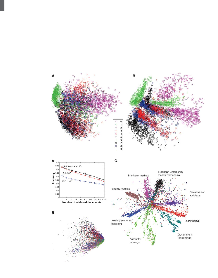
Fig. 3. (A) The two-
dimensional codes for 500
digits of each class produced
by taking the first two prin-
cipal components of all
60,000 training images.
(B) The two-dimensional
codes found by a 784-
1000-500-250-2 autoen-
coder. For an alternative
visualization, see (8).

Fig. 4. (A) The fraction of
retrieved documents in the
same class as the query when
a query document from the
test set is used to retrieve other
test set documents, averaged
over all 402,207 possible que-
ries. (B) The codes produced
by two-dimensional LSA. (C)
The codes produced by a 2000-
500-250-125-2 autoencoder.

REPORTS

28 JULY 2006

VOL 313

SCIENCE

www.sciencemag.org

506

times as desired. It can be shown that adding an
extra layer always improves a lower bound on
the log probability that the model assigns to the
training data, provided the number of feature
detectors per layer does not decrease and their
weights are initialized correctly (9). This bound
does not apply when the higher layers have
fewer feature detectors, but the layer-by-layer
learning algorithm is nonetheless a very effec-
tive way to pretrain the weights of a deep auto-
encoder. Each layer of features captures strong,
high-order correlations between the activities of
units in the layer below. For a wide variety of
data sets, this is an efficient way to pro-
gressively reveal low-dimensional, nonlinear
structure.

After pretraining multiple layers of feature

detectors, the model is

Bunfolded[ (Fig. 1) to

produce encoder and decoder networks that
initially use the same weights. The global fine-
tuning stage then replaces stochastic activities
by deterministic, real-valued probabilities and
uses backpropagation through the whole auto-
encoder to fine-tune the weights for optimal
reconstruction.

For continuous data, the hidden units of the

first-level RBM remain binary, but the visible
units are replaced by linear units with Gaussian
noise (10). If this noise has unit variance, the
stochastic update rule for the hidden units
remains the same and the update rule for visible
unit i is to sample from a Gaussian with unit
variance and mean b

i

þ

P

j

h

j

w

ij

.

In all our experiments, the visible units of

every RBM had real-valued activities, which
were in the range

E0, 1^ for logistic units. While

training higher level RBMs, the visible units
were set to the activation probabilities of the
hidden units in the previous RBM, but the
hidden units of every RBM except the top one
had stochastic binary values. The hidden units
of the top RBM had stochastic real-valued
states drawn from a unit variance Gaussian
whose mean was determined by the input from
that RBM

_s logistic visible units. This allowed

the low-dimensional codes to make good use of
continuous variables and facilitated compari-
sons with PCA. Details of the pretraining and
fine-tuning can be found in (8).

To demonstrate that our pretraining algo-

rithm allows us to fine-tune deep networks
efficiently, we trained a very deep autoen-
coder on a synthetic data set containing
images of

Bcurves[ that were generated from

three randomly chosen points in two di-
mensions (8). For this data set, the true in-
trinsic dimensionality is known, and the
relationship between the pixel intensities and
the six numbers used to generate them is
highly nonlinear. The pixel intensities lie
between 0 and 1 and are very non-Gaussian,
so we used logistic output units in the auto-
encoder, and the fine-tuning stage of the
learning minimized the cross-entropy error
E–

P

i

p

i

log ˆp

i

–

P

i

(1 – p

i

) log(1 –

g

ˆp

i

)

^, where

p

i

is the intensity of pixel i and

g

ˆp

i

is the

intensity of its reconstruction.

The autoencoder consisted of an encoder

with layers of size (28

28)-400-200-100-

50-25-6 and a symmetric decoder. The six
units in the code layer were linear and all the
other units were logistic. The network was
trained on 20,000 images and tested on 10,000
new images. The autoencoder discovered how
to convert each 784-pixel image into six real
numbers that allow almost perfect reconstruction
(Fig. 2A). PCA gave much worse reconstruc-
tions. Without pretraining, the very deep auto-
encoder always reconstructs the average of the
training data, even after prolonged fine-tuning
(8). Shallower autoencoders with a single
hidden layer between the data and the code
can learn without pretraining, but pretraining
greatly reduces their total training time (8).
When the number of parameters is the same,
deep autoencoders can produce lower recon-
struction errors on test data than shallow ones,
but this advantage disappears as the number of
parameters increases (8).

Next, we used a 784-1000-500-250-30 auto-

encoder to extract codes for all the hand-
written digits in the MNIST training set (11).
The Matlab code that we used for the pre-
training and fine-tuning is available in (8). Again,
all units were logistic except for the 30 linear
units in the code layer. After fine-tuning on all
60,000 training images, the autoencoder was
tested on 10,000 new images and produced
much better reconstructions than did PCA
(Fig. 2B). A two-dimensional autoencoder
produced a better visualization of the data
than did the first two principal components
(Fig. 3).

We also used a 625-2000-1000-500-30 auto-

encoder with linear input units to discover 30-
dimensional codes for grayscale image patches
that were derived from the Olivetti face data set
(12). The autoencoder clearly outperformed
PCA (Fig. 2C).

When trained on documents, autoencoders

produce codes that allow fast retrieval. We rep-
resented each of 804,414 newswire stories (13)
as a vector of document-specific probabilities
of the 2000 commonest word stems, and we
trained a 2000-500-250-125-10 autoencoder on
half of the stories with the use of the multiclass
cross-entropy error function

E–

P

i

p

i

log

g

ˆp

i

^ for

the fine-tuning. The 10 code units were linear
and the remaining hidden units were logistic.
When the cosine of the angle between two codes
was used to measure similarity, the autoencoder
clearly outperformed latent semantic analysis
(LSA) (14), a well-known document retrieval
method based on PCA (Fig. 4). Autoencoders
(8) also outperform local linear embedding, a
recent nonlinear dimensionality reduction algo-
rithm (15).

Layer-by-layer pretraining can also be used

for classification and regression. On a widely used
version of the MNIST handwritten digit recogni-

tion task, the best reported error rates are 1.6% for
randomly initialized backpropagation and 1.4%
for support vector machines. After layer-by-layer
pretraining in a 784-500-500-2000-10 network,
backpropagation using steepest descent and a
small learning rate achieves 1.2% (8). Pretraining
helps generalization because it ensures that most
of the information in the weights comes from
modeling the images. The very limited informa-
tion in the labels is used only to slightly adjust
the weights found by pretraining.

It has been obvious since the 1980s that

backpropagation through deep autoencoders
would be very effective for nonlinear dimen-
sionality reduction, provided that computers
were fast enough, data sets were big enough,
and the initial weights were close enough to a
good solution. All three conditions are now
satisfied. Unlike nonparametric methods (15, 16),
autoencoders give mappings in both directions
between the data and code spaces, and they can
be applied to very large data sets because both
the pretraining and the fine-tuning scale linearly
in time and space with the number of training
cases.

References and Notes

1. D. C. Plaut, G. E. Hinton, Comput. Speech Lang. 2, 35

(1987).

2. D. DeMers, G. Cottrell, Advances in Neural Information

Processing Systems 5 (Morgan Kaufmann, San Mateo, CA,
1993), pp. 580–587.

3. R. Hecht-Nielsen, Science 269, 1860 (1995).
4. N. Kambhatla, T. Leen, Neural Comput. 9, 1493

(1997).

5. P. Smolensky, Parallel Distributed Processing: Volume 1:

Foundations, D. E. Rumelhart, J. L. McClelland, Eds. (MIT
Press, Cambridge, 1986), pp. 194–281.

6. G. E. Hinton, Neural Comput. 14, 1711 (2002).
7. J. J. Hopfield, Proc. Natl. Acad. Sci. U.S.A. 79, 2554

(1982).

8. See supporting material on Science Online.
9. G. E. Hinton, S. Osindero, Y. W. Teh, Neural Comput. 18,

1527 (2006).

10. M. Welling, M. Rosen-Zvi, G. Hinton, Advances in Neural

Information Processing Systems 17 (MIT Press, Cambridge,
MA, 2005), pp. 1481–1488.

11. The MNIST data set is available at http://yann.lecun.com/

exdb/mnist/index.html.

12. The Olivetti face data set is available at www.

cs.toronto.edu/ roweis/data.html.

13. The Reuter Corpus Volume 2 is available at http://

trec.nist.gov/data/reuters/reuters.html.

14. S. C. Deerwester, S. T. Dumais, T. K. Landauer, G. W.

Furnas, R. A. Harshman, J. Am. Soc. Inf. Sci. 41, 391
(1990).

15. S. T. Roweis, L. K. Saul, Science 290, 2323 (2000).
16. J. A. Tenenbaum, V. J. de Silva, J. C. Langford, Science

290, 2319 (2000).

17. We thank D. Rumelhart, M. Welling, S. Osindero, and

S. Roweis for helpful discussions, and the Natural
Sciences and Engineering Research Council of Canada for
funding. G.E.H. is a fellow of the Canadian Institute for
Advanced Research.

Supporting Online Material

www.sciencemag.org/cgi/content/full/313/5786/504/DC1
Materials and Methods
Figs. S1 to S5
Matlab Code

20 March 2006; accepted 1 June 2006
10.1126/science.1127647

REPORTS

www.sciencemag.org

SCIENCE

VOL 313

28 JULY 2006

507