AMG -
1 cycle

True
Solution

Initial Value

Prepared in cooperation with the
U.S. Department of Energy

MODFLOW-2000, THE U.S. GEOLOGICAL SURVEY
MODULAR GROUND-WATER MODEL—USER GUIDE TO THE
LINK-AMG (LMG) PACKAGE FOR SOLVING MATRIX
EQUATIONS USING AN ALGEBRAIC MULTIGRID SOLVER

Open-File Report 01-177

U.S. Department of the Interior
U.S. Geological Survey

MODFLOW-2000, THE U.S. GEOLOGICAL SURVEY
MODULAR GROUND-WATER MODEL – USER GUIDE TO THE
LINK-AMG (LMG) PACKAGE FOR SOLVING MATRIX
EQUATIONS USING AN ALGEBRAIC MULTIGRID SOLVER

By STEFFEN W. MEHL and MARY C. HILL

U.S. GEOLOGICAL SURVEY

Open-File Report 01-177

Prepared in cooperation with the
U.S. Department of Energy

Denver, Colorado

2001

U.S. DEPARTMENT OF THE INTERIOR

GALE A. NORTON, Secretary

U.S. GEOLOGICAL SURVEY

Charles G. Groat, Director

The use of trade, product, industry, or firm names is for descriptive purposes only and does not imply
endorsement by the U.S. Government.
____________________________________________________________________________________
For additional information write to:

Regional Research Hydrologist
U.S. Geological Survey
Box 25046, Mail Stop 413
Denver Federal Center
Denver, CO 50225-0046

Copies of this report can be
purchased from:

U.S. Geological Survey
Branch of Information Services
Box 25286
Denver, CO 50225-0425

iii

PREFACE

This report describes a computer program that links MODFLOW-2000, the U.S

Geological Survey modular three-dimensional finite-difference ground-water model, with an
advanced technique for solving matrix equations, the freeware algebraic multigrid (AMG) solver
produced by the GMD - German National Research Center for Information Technology. The
AMG solver can be downloaded from the Internet URL at

http://www.mgnet.org/mgnet/Codes/gmd/amg.tgz

, where the version used in this report is

identified as AMG1R5. For convenience it is also distributed with MODFLOW-2000. The AMG
solver is, however, produced by GMD and, though freely distributed, is subject to restrictions
defined by GMD. One of those restrictions is that GMD must be acknowledged in publications
for which results were produced using the algebraic multigrid solver. The U.S. Geological Survey
encourages users to respect this restriction. While this is the only restriction that will apply to
most users, those using the algebraic multigrid solver in any other way should consult with GMD
about additional restrictions.

More recent developments in AMG software not available for free may be available from

a variety of vendors, and users may wish to consider these resources. These algorithms are more
sophisticated and, as a result, are more efficient in their use of computer memory. In using such
alternatives, the implementation provided by the Link-AMG (LMG) Package described in this
report to make the AMG1R5 solver work with MODFLOW may be useful.

The performance of the program has been tested in a variety of applications. Future

applications, however, might reveal errors that were not detected in the test simulations. Users are
requested to notify the U.S. Geological Survey of any errors found in this document or the
computer program using the email address available at the web address below. Updates might
occasionally be made to both this document and to LMG. Users can check for updates on the
Internet at URL http://water.usgs.gov/software/ground_water.html/.

iv

CONTENTS

Abstract ............................................................................................................................... 1

Introduction ......................................................................................................................... 2

Purpose and Scope ....................................................................................................................... 2

Acknowledgments ........................................................................................................................ 3

Brief Description of the Algebraic Multigrid (AMG) Solver ............................................. 4

Implementation of AMG in MODFLOW-2000 Using the Link-AMG (LMG)

Package........................................................................................................................... 10

Solution of Nonlinear Problems Using Picard Iterations ........................................................... 10

Convergence Criterion ............................................................................................................... 10

Tips for Achieving Convergence ............................................................................................... 11

BCLOSE and MXITER ......................................................................................................... 11

MXCYC ................................................................................................................................. 12

ICG......................................................................................................................................... 12

DAMP .................................................................................................................................... 13

Comparison of LMG with PCG2 for Ground-Water Flow Problems ............................... 16

Compatibility, Portability and Memory Requirements ..................................................... 18

Compatibility and Portability ..................................................................................................... 18

Memory Requirements ............................................................................................................... 18

Input Instructions and Sample Data Inputs ....................................................................... 20

Input Instructions........................................................................................................................ 20

Sample Data Inputs .................................................................................................................... 22

Brief Program Description ................................................................................................ 23

Narrative for Module LMG1AL................................................................................................. 23

List of Variables for Module LMG1AL..................................................................................... 23

Narrative for Module LMG1RP ................................................................................................. 25

List of Variables for Module LMG1RP ..................................................................................... 25

Narrative for Module LMG1AP................................................................................................. 26

List of Variables for Module LMG1AP ..................................................................................... 27

Narrative for Module ADAMP1 ................................................................................................ 30

List of Variables for Module ADAMP1..................................................................................... 30

Narrative for Module ADAMP2 ................................................................................................ 30

List of Variables for Module ADAMP2..................................................................................... 31

References ......................................................................................................................... 32

v

FIGURES

Figure 1. Diagram showing the reduction of errors in the solution to a one-dimensional

flow problem with constant head boundaries of zero at both ends.. ........................................ 5

Figure 2. Diagram showing the propagation of the head solution for a homogenous

aquifer with a single injection well located at the center of 31x31 grid, with constant
head boundaries of 0.05 along the perimeter.. ......................................................................... 8

TABLES

Table 1. Comparison of computational differences between the PCG2 and LMG solvers

for several ground-water flow problems. ............................................................................... 16

Table 2. Arrays used in AMG1R5, their dimensions, the user-defined variables that

control the storage allocated for the arrays, values recommended by Ruge and others
(1990), and the global storage arrays in MODFLOW-2000 in which the AMG1R5
arrays are stored. .................................................................................................................... 18

1

MODFLOW-2000,

THE U.S. GEOLOGICAL SURVEY MODULAR

GROUND-WATER MODEL --

USER GUIDE TO THE LINK-AMG (LMG) PACKAGE FOR

SOLVING MATRIX EQUATIONS USING AN ALGEBRAIC

MULTIGRID SOVLER

By Steffen W. Mehl and Mary C. Hill

Abstract

This report documents the Link-AMG (LMG) Package that links MODFLOW-

2000, the U.S. Geological Survey modular, transient, three-dimensional, finite-difference
ground-water flow model, to an algebraic multigrid (AMG) solver for matrix equations.
The LMG Package has some distinct advantages over other solvers available with
MODFLOW-2000 for problems with large grids (more than about 40,000 cells) and (or)
a highly variable hydraulic-conductivity field. Experience has indicated that, in such
problems, execution times using the AMG solver are typically about 2 to 25 times faster
than execution times using MODFLOW’s PCG2 Package with the modified incomplete
Cholesky preconditioner. The drawback to the AMG method used in LMG is the
relatively large amount of computer memory required. In problems simulated for this
work, the AMG solver used typically required 3 to 8 times more memory than PCG2. For
one 465,600-node problem, for example, 151 megabytes (MB) of memory were required
when the LMG package was used, whereas PCG2 required 47 MB of memory. The
execution time, however, decreased from 942 seconds to 50 seconds, so there is a clear
trade-off between execution time and memory requirements. On modern computers, such
memory requirements are becoming increasingly attainable.

This report provides a brief description of the AMG method used, an explanation

of the convergence criterion, a discussion of its memory requirements, some performance
comparisons, and sample data inputs. In addition, detailed instructions on how the LMG
Package links the AMG code to MODFLOW-2000 are provided.

2

Introduction

Ground-water modelers are constantly challenged by trying to represent

realistically complicated natural systems using numerical models. Increased detail means
larger model grids and longer execution times. In addition, increasingly complicated
processes and methods for exploring model results, such as Monte-Carlo simulation and
model calibration, make reduction of computer execution time extremely desirable.
Reduction in computer execution time provides an opportunity for ground-water
modelers to investigate their systems more thoroughly and in ways not previously
possible. In recent decades, computer models of ground-water systems have taken
advantage of improved processor speeds, but have not, in general, taken advantage as
effectively of increased memory availability, other than increasing the number of grid
nodes.

Algebraic multigrid solvers can attain significant reduction in computer execution

time for many problems. Generally, the decrease in execution time is accompanied by the
use of larger amounts of memory. The pioneering work that developed the theory behind
algebraic multigrid methods took place in the early 1980s, and computer memory has
evolved to where these methods can be used by a wide audience. The present report
makes an algebraic multigrid (AMG) solver produced by GMD (German National
Research Center for Information Technology) available for users of MODFLOW-2000,
the U.S. Geological Survey modular, three-dimensional, finite-difference ground-water
model.

The AMG solver is included in MODFLOW-2000 as distributed by the U.S.

Geological Survey. When the Link-AMG (LMG) Package is activated through the Name
file using file type LMG, the AMG solver is used to solve the equations produced by
MODFLOW-2000s Ground-Water Flow Process for hydraulic head, and, if applicable,
the equations produced by MODFLOW-2000s Sensitivity Process for sensitivities of
hydraulic head throughout the grid. Linear or nonlinear flow conditions may be
simulated.

Purpose and Scope

The purpose of this report is to document LMG, a program that links a freeware

version of GMD’s algebraic multigrid solver (AMG1R5), to MODFLOW-2000. This
report provides a brief description of the AMG method used, an explanation of the
convergence criterion, a discussion of its memory requirements, some performance
comparisons, and sample data inputs. In addition, detailed instructions on how the LMG
Package links the AMG code to MODFLOW-2000 are provided. This report was
prepared in cooperation with the U.S. Department of Energy.

3

Acknowledgments

The authors wish to acknowledge Professor Hari Rajaram, Dr. Russell Detwiler,

Professor Steve McCormick, and Dr. John Ruge of the University of Colorado at
Boulder, who introduced us to the algebraic multigrid solver and helped make the LMG
Package. We especially appreciate the efforts made on our behalf by Klaus Stüben of
GMD, who helped resolve several difficulties. We are grateful for the reviews provided
by Leonard Konikow and Cory Angeroth of the U.S. Geological Survey, which improved
the quality of this report. Finally, we thank the German people and government who,
through their tax dollars and foresight, funded the development of this solver and made it
freely available.

4

Brief Description of the Algebraic Multigrid (AMG) Solver

Ruge and others (1990) developed the AMG solver, AMG1R5, implemented by

the LMG package. This USGS report highlights the general features of the AMG solver;
for more detail refer to Stüben (1999, 2001) and Ruge and Stüben (1987). In addition,
Briggs and others (2000) provide an excellent treatment of multigrid methods, and much
of this overview is based on their discussion of the subject.

The characteristics of the AMG solver are described by considering its

performance relative to alternative solvers using two small problems. The alternative
solvers considered are successive over-relaxation (SOR), strongly implicit procedure
(SIP), and the preconditioned conjugate-gradient method (PCG). The implementation of
the SOR and SIP solvers is described by McDonald and Harbaugh (1988), the
implementation of the PCG solver is described by Hill (1990), and the implementation of
the AMG solver is described in this work. These implementations are all for
MODFLOW. The performance of all the solvers is compared for both problems, and the
differences are used to illustrate the characteristics of the AMG solver. While these small,
simple problems can be solved quickly using the alternate solvers considered, for large,
complicated problems the characteristics of the AMG solver illustrated can result in much
faster execution times.

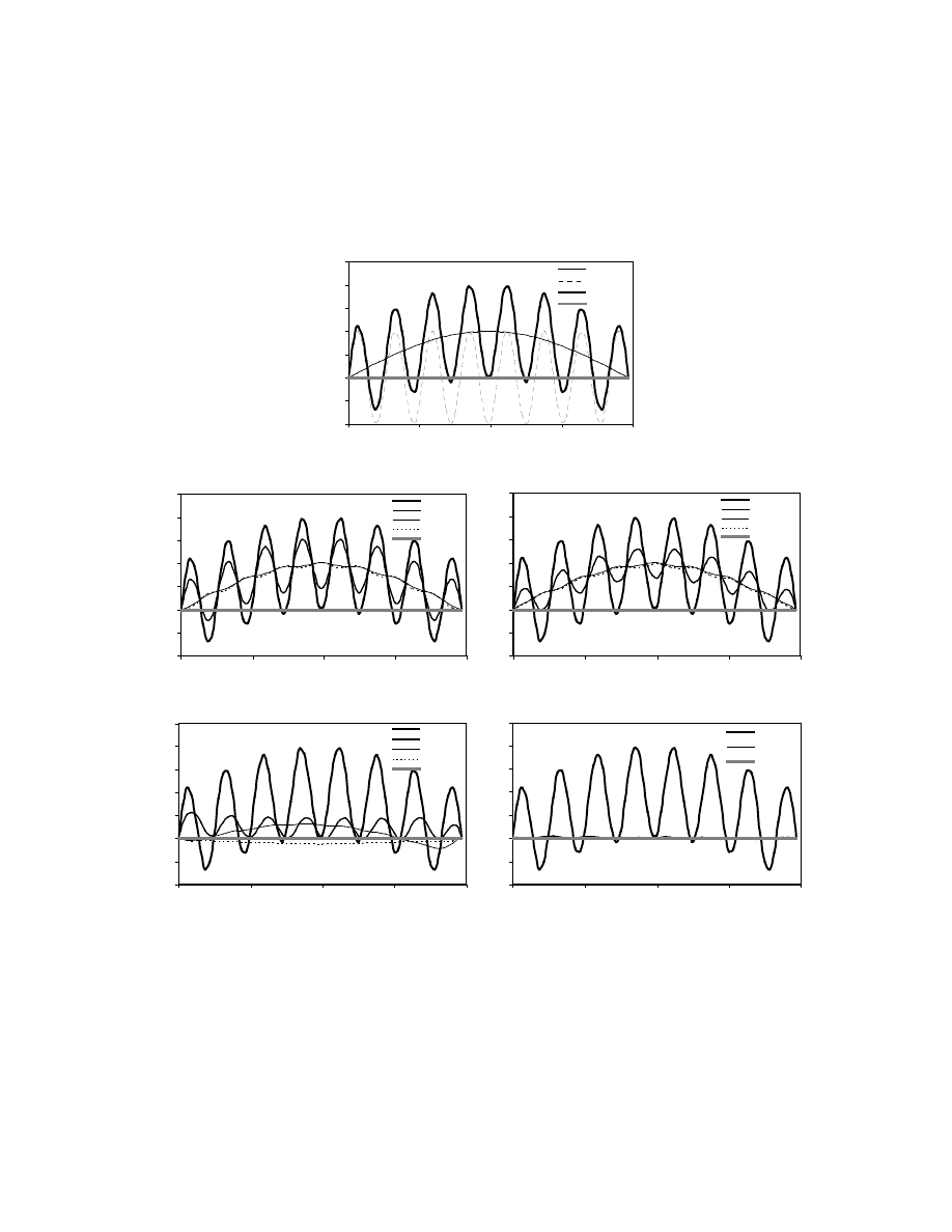
The performance of the SOR, SIP, and PCG2 solvers is heavily dependent on the

initial head distribution. These solvers generally remove high frequency, highly
oscillatory errors most effectively (particularly SOR). Thus, the convergence properties
of these solvers depend on how oscillatory the error in the solution is. If the error is very
oscillatory (such as the k=15 error in figure 1a), these solvers converge quickly. In
contrast, if the error is relatively smooth (such as the k=1 error in figure 1a), these solvers
will converge much more slowly. If the error contains components that are very
oscillatory and other components that are smooth (such as the k=1+15 error in figure 1a),
most of the oscillatory components will be removed after a few iterations, but the smooth
error components will remain virtually unchanged. The slow reduction of smooth error
components is what plagues the performance of these solvers. Thus, a good initial head
distribution, which is equivalent to being void of smooth error components, is needed for
rapid convergence.

The first problem was designed to illustrate the concept of reduction of error

components. This problem represents one-dimensional flow with constant-head
boundaries at both ends fixed at a value of zero. There is no gradient through the system,
and the true solution is a value of zero throughout the domain (figure 1a). By using an
initial head other than zero, one can examine how the solvers change this head to zero,
the correct solution. To produce a problem that would emphasize the difference between
the SOR, SIP, and PCG solvers and the AMG solver, the initial head for this problem was
constructed by adding smooth and oscillatory error components, shown in figure 1a. The
smooth component is the first wave number (k=1), while the oscillatory component is the
fifteenth wave (k=15). Figures 1b and 1c show that the SOR and the SIP remove most of
the high-frequency error after just two iterations, but the smooth error component is
essentially unchanged. Figure 1d shows that the PCG solver with the modified
incomplete Cholesky preconditioner makes much better progress reducing the error

5

components, but a smooth error component remains in the solution after three iterations.
In contrast, the AMG solution shown in figure 1e reduces both the smooth and the
oscillatory error in one cycle. The computation effort of one AMG cycle, however, is
greater than one iteration of the other solvers, as explained later.

Figure 1. Errors in the solution to a one-dimensional flow problem with constant head boundaries

of zero at both ends. (a) Components of initial head (errors), with smooth (k=1) and
oscillatory (k=15) components. Reduction of error components for the (b) SOR, (c) SIP,
(d) PCG2 with the modified incomplete Cholesky (MIC) preconditioner, and (e) AMG
solvers.

Error Frequencies of Initial Head

-1

-0.5

0

0.5

1

1.5

2

2.5

0

16

32

48

64

node

er

ro

r

k=1

k=15

k= 1 + 15

T rue Solution

Convergence of the PCG (MIC) Solution

-1

-0.5

0

0.5

1

1.5

2

2.5

0

16

32

48

64

node

er

ro

r

iter=0

iter=1

iter=2
iter=3

T rue Solution

Convergence of the SOR Solution

-1

-0.5

0

0.5

1

1.5

2

2.5

0

16

32

48

64

node

er

ro

r

iter=0
iter=1
iter=2
iter=3
T rue Solution

Convergence of the SIP Solution

-1

-0.5

0

0.5

1

1.5

2

2.5

0

16

32

48

64

node

er

ro

r

iter=0
iter=1
iter=2
iter=3
T rue Solution

Convergence of the AMG Solution

-1

-0.5

0

0.5

1

1.5

2

2.5

0

16

32

48

64

node

er

ro

r

cycle=0

cycle=1

T rue Solution

a

b

c

d

e

6

There are two key ideas that result in multigrid methods being able to solve some

problems so quickly. The first is that they exploit the rapid reduction of highly oscillatory
error components by iterative solvers, such as the SOR. The second is that they solve the
same problem on several different grids that are coarser than the initial grid. Errors that
appear smooth on a finer grid will appear more oscillatory on a coarser grid and, thus, can
be reduced more effectively on a coarser grid. The number of grids, the grid sizes, and
the iterative solver used for each grid are selected such that the full range of error
components are represented at a frequency that the particular solver eliminates quickly.
Thus, by cycling between the different grids, all components of the error at all
frequencies are reduced efficiently.

Another way to look at the solution characteristics is that the SOR, SIP, and PCG

solvers calculate the updated head solution at a given node by various forms of averaging
with the head solution at the neighboring nodes. This means that information is only
propagated efficiently to close neighboring cells. Although solutions for each grid of a
multigrid method are obtained using iterative solvers, multigrid methods propagate
information more effectively throughout the system because some of the grids used are
coarser. This has the effect of causing neighboring cell centers to be further away from
each other in space, and the information is propagated a further distance.

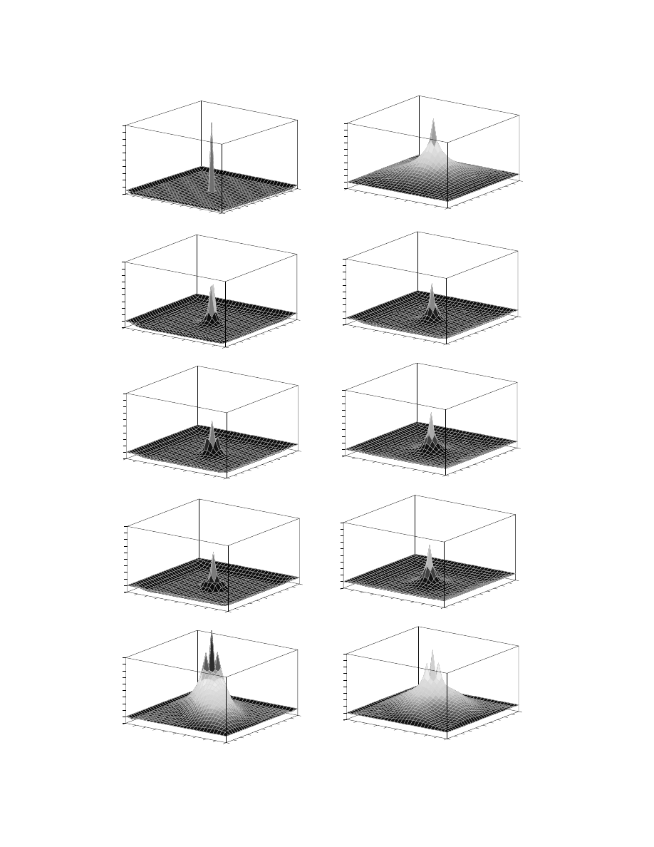
The second problem illustrates how the solvers propagate information through the

grid by examining the evolution of the head solution in a two-dimensional aquifer. The
aquifer is homogenous with a single injection well at the center of a 31x31 grid and
constant-head boundaries of 0.05 along the perimeter. The initial value is zero internally,
except at the location of the well where it has a value of unity (figure 2a). By examining
the true solution (figure 2b), one can see that the solvers need to increase the head
throughout the interior of the domain, except at the injection well where the head needs to
be decreased. Solutions after one and two iterations are shown for SOR, SIP, and PCG
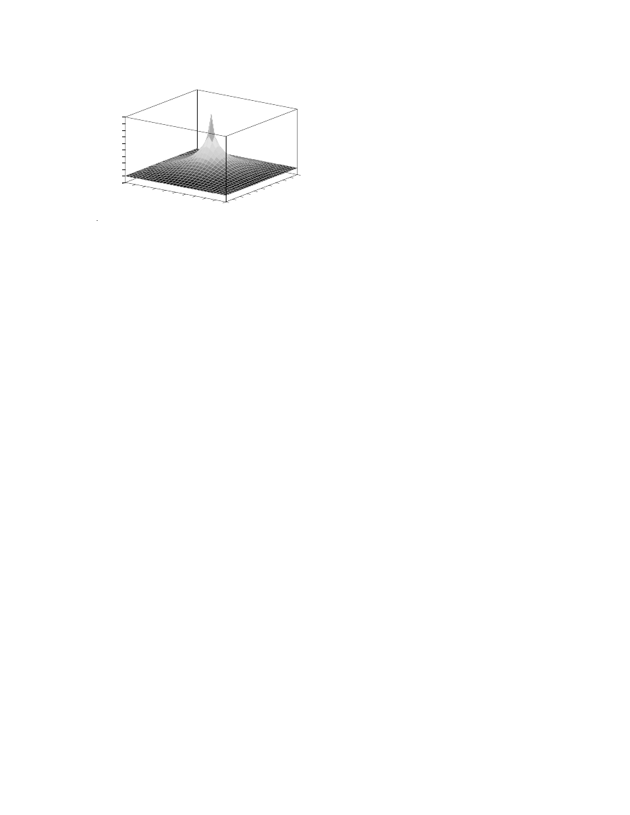
with the two preconditioners included in PCG2 (Hill, 1990). The AMG solution after one
cycle also is shown. Figure 2 illustrates three characteristics of these solvers: (1) The
SIP, SOR, and PCG solvers are limited in how much distant cells can be influenced at
each iteration so that information is mostly propagated locally in space. (2) For PCG, the
type of preconditioning is important as the modified incomplete Cholesky preconditioner
allows the PCG to influence more distant cells and thus propagate information a farther
distance. (3) The AMG solver is able to propagate information throughout the entire grid
in one cycle.

7

0.50

0.25

0.00

Head

0.0

0.5

1.0

Y

1.0

0.5

0.0

X

0.50

0.25

0.00

Head

0.0

0.5

1.0

Y

1.0

0.5

0.0

X

0.50

0.25

0.00

Head

0.0

0.5

1.0

Y

1.0

0.5

0.0

X

0.50

0.25

0.00

Head

0.0

0.5

1.0

Y

1.0

0.5

0.0

X

0.50

0.25

0.00

Head

0.0

0.5

1.0

Y

1.0

0.5

0.0

X

0.50

0.25

0.00

Head

0.0

0.5

1.0

Y

1.0

0.5

0.0

X

0.50

0.25

0.00

Head

0.0

0.5

1.0

Y

1.0

0.5

0.0

X

0.50

0.25

0.00

Head

0.0

0.5

1.0

Y

1.0

0.5

0.0

X

0.50

0.25

0.00

Head

0.0

0.5

1.0

Y

1.0

0.5

0.0

X

1.0

0.5

0.0

Head

0.0

0.5

1.0

Y

1.0

0.5

0.0

X

j

i

g

e

c

h

f

d

b

true solution

SOR

1 iteration

2 iterations

2 iterations

2 iterations

2 iterations

SIP

1 iteration

PCG (Polynomial)

1 iteration

PCG (MIC)

1 iteration

a

initial value

Head

8

Figure 2. Head solution for a homogenous aquifer with a single injection well located at the

center of 31x31 grid, with constant head boundaries of 0.05 along the perimeter. (a)
initial value, (b) true solution, (c and d) SOR solution after 1 and 2 iterations, (e and f)
SIP solution after 1 and 2 iterations, (g and h) PCG solution with the polynomial
preconditioner after 1 and 2 iterations, (i and j) PCG solution with the MIC
preconditioner after 1 and 2 iterations, (k) AMG solution after 1 cycle.

These small example problems were chosen for illustrative purposes; in these

simple cases, the speed of the SOR, SIP, and PCG iterations relative to one AMG cycle
means that the AMG is actually slower. This is because one multigrid cycle takes longer
than one iteration of the SOR, SIP, or PCG, which is because one cycle involves multiple
iterations on several different grids, as described below. However, examples shown later
demonstrate that AMG attains smaller execution times for many large, complicated
problems.

Geometric multigrid solvers work by taking the original problem and creating a

series of associated, successively coarser grid representations. Approximate solutions are
produced first for the finest grid considered, then on the next coarsest, on down to the
coarsest grid representation. The solution on the coarsest grid is used to correct the
solution at the next finest grid. This process is applied recursively such that corrections
from a coarse grid to the next finest grid are applied until the finest grid is reached. Each
of the cycles mentioned previously are composed of one such sequence. Convergence is
checked and additional cycles are performed as needed.

The advantages of multigrid methods over the other iterative solvers mentioned

are: (1) the effectiveness of the multigrid solver is not as dependent on the initial head
distribution and (2) for many problems of interest, the rate of convergence scales
approximately linearly with the size of the domain, unlike the other solvers where the rate
of convergence increases nonlinearly (Demmel, 1997, p. 277). Thus, for many larger
problems, multigrid methods can be extremely effective. One disadvantage of multigrid
methods compared to the other iterative solvers mentioned is that information needs to be
stored on more than a single grid so that the memory requirements for multigrid methods
generally are greater than for other iterative solvers. This is probably one of the reasons
why, historically, multigrid methods have not been popular for ground-water models,
which tend to require considerable memory even when the alternative solvers are used. In
addition, developing robust ways to interpolate values across several grids (especially in

0.50

0.25

0.00

Head

0.0

0.5

1.0

Y

1.0

0.5

0.0

X

k

AMG

1 cycle

9

three dimensions) when the discretization involves complex grid geometries has been
difficult.

Geometric multigrid methods directly use information about the physical model

grid to determine how to coarsen the grid and how to interpolate between the grids. These
methods often fail given the complexity found in the broad range of ground-water flow
problems that occur in practice. In contrast, algebraic multigrid (AMG) methods address
this latter shortcoming and are not limited by complex grid geometries (Ruge and Stüben,
1987). The underlying idea of AMG is the same (fast reduction of smooth error
components), but instead of coarsening the physical grid and applying a particular solver
for that grid, AMG methods use a simple solver (typically Gauss-Seidel) and coarsen the
matrix. That is, the coefficients of the matrix itself are used to determine where to
coarsen and in which direction, such that the solver will be effective at each level of
coarsening. Thus, no information about the grid or physical geometry is required beyond
what is already contained in the coefficient matrix. Wagner and others (1997) used a
similar approach, in which the multigrid solver incorporated algebraic information, to
simulate ground-water flow and transport through several hydraulic-conductivity fields.
They showed that their technique was able to solve problems where standard multigrid
methods failed.

AMG methods generally use more memory and are not quite as efficient as

geometric multigrid methods when the latter work, but the AMG methods successfully
solve a broader class of problems, and this robust behavior makes them much more
useful.

10

Implementation of AMG in MODFLOW-2000 Using the Link-AMG

(LMG) Package

The AMG routine from the GMD (referred to by GMD as AMG1R5) was not

modified. Instead, a package was written to interface MODFLOW-2000 with the AMG
solver. This package is called Link-AMG (LMG) and is activated by including file type
LMG in the name file as described by Harbaugh and others (2000, p. 7, 43-44). The
actual equation solution is performed by calls from the LMG to the AMG1R5 routine.
Nonlinear problems are solved using Picard iterations. A key difference between the
LMG package and the other MODFLOW-2000 solver packages is how convergence is
controlled. The implementation of Picard iterations and convergence control are
discussed in the following sections.

Solution of Nonlinear Problems Using Picard Iterations

Nonlinear solutions for hydraulic head are produced by MODFLOW when model

layers are simulated as being convertible and when some types of boundary conditions
are used. For example, the River Package changes the calculation of flow to the ground-
water system when the hydraulic head falls beneath the elevation defined as the bottom of
the riverbed (McDonald and Harbaugh, 1988, ch. 6; Hill and others, 2000, p. 45). When
the solution for hydraulic heads is nonlinear, the solver needs to solve a sequence of
matrix equations, each using different, updated values of hydraulic heads to evaluate
nonlinear terms. This continues until the updated hydraulic heads match the last set, using
the convergence criterion as described below. The LMG Package solves nonlinear
problems using Picard iterations, which is the same technique that the other MODFLOW
solvers use. Picard iterations update the hydraulic heads for each solution in the sequence
by simply using the hydraulic heads from the end of the last solution to calculate the
equations for the subsequent solution.

Convergence Criterion

The AMG solver uses a scaled L

2

norm (the Euclidean norm) of the residual

vector to measure how well a head distribution satisfies the matrix equations. To obtain a
formulation for which the convergence criterion value has physical meaning and so that
similar values can be used for most systems, scaling is needed. The scaling used in the
LMG Package is described in this section.

Calculation of the scaled L

2

norm of the residual vector first requires the residual

vector, which is calculated as

{ }

[ ]

{ }

{ }

f

h

A

r

k

−

=

,

(1)

where

{r} is the N x 1-dimensional residual vector [L

3

/T if the solution is for hydraulic head];

N is the number of nodes in the finite-difference grid;

11

[A] is the N

×

N-dimensional coefficient matrix calculated as described by McDonald and

Harbaugh (1988) and Harbaugh and others (2000) or, for sensitivities, as
described by Hill and others (2000) [L

2

/T if the solution is for hydraulic head];

{h

k

} is an N-dimensional vector of hydraulic heads or sensitivities at the kth time step [L

if the solution is for hydraulic head]; and

{f} is a vector of pumpage and terms related to other stresses and boundary conditions as

defined by McDonald and Harbaugh (1988) and Harbaugh and others (2000) or,
for sensitivities, as described by Hill and others (2000) [L

3

/T if the solution is for

hydraulic head].

The L

2

norm of the residual vector is calculated as:

{ }

2

/

1

1

2

2













=

∑

=

N

i

i

r

r

,

(2)

where r

i

is the ith element of vector {r}. This norm is then scaled by dividing by the

average value of the absolute value of the right hand side vector,

{ }

f . When

{ }

{ }

ε

≤

f

r

2

,

(3)

where

ε

[L

3

/T] is the user specified tolerance BCLOSE, convergence is achieved. This

criterion and scaling is similar to that used by Kipp and others (1998, eq. 25) to solve the
matrix equations related to dispersive transport.

In the Picard iterations used to solve nonlinear problems, the coefficient matrix

[A] and the right-hand-side vector {f} are updated after each iteration using the updated
head solution. If the head solution continues to meet the convergence criterion after the
equations are updated, convergence is achieved. If the criterion is no longer met, the
solver is used to find a new head solution to the updated equations.

Tips for Achieving Convergence

There are a number of variables defined by the user that can affect the

performance of the AMG solver. They are BCLOSE, the convergence criterion;
MXITER, the maximum number of calls to the AMG routine; MAXCYC, the number of
multigrid cycles performed per call to the AMG routine; ICG, a flag controlling the use
of conjugate gradient iterations at the end of each multigrid cycle, and DAMP, which can
be used to make the solution change more slowly and can be useful for nonlinear
problems. Each of these variables is discussed below.

BCLOSE and MXITER

The AMG routine is called iteratively until the convergence criterion BCLOSE is

met or the number of iterations has exceeded MXITER (equivalent to MXITER of PCG2;
Hill, 1990). A convergence criterion value that is too large can be detected in

12

MODFLOW-2000 by unacceptably large global ground-water flow budget errors,
sensitivity errors, or both. If such problems exist, BCLOSE should be decreased.
Typically, decreasing BCLOSE by one order of magnitude will decrease the global
budget error by about one order of magnitude.

A value of BCLOSE that is smaller than is needed will produce excessively long

execution times. Such a situation probably exists if the global budget errors calculated for
the solutions at all time steps and all parameters (if sensitivities are calculated) are less
than 0.01 percent (0.00 will be printed by MODFLOW-2000 as the percent discrepancy
for all budgets). If this occurs, BCLOSE can be increased incrementally by about an
order of magnitude at each increment until the largest global budget error equals about
0.01 percent.

Another situation can occur where the solver fails to converge because BCLOSE

is set too small. This can be detected by examining the residuals after each cycle
(IOUTAMG=3) to see if the solver fails to lower the residuals any further after a certain
number of cycles. When BCLOSE is too small, the closure criterion is below the limit of
the round-off error in the calculations for this particular problem, and the solver cannot
improve the solution any further. For this reason, the average value of the absolute value

of the right hand side vector,

{ }

f , which is used to scale the L

2

norm, is also printed. The

user has a reference point in that BCLOSE should not be chosen such that, when scaled,
it is less than the limit of the solver for this problem.

MXITER is the maximum number of times that the AMG routines will be called

to obtain a solution. MXITER is never less than 2 and rarely more than 50. MXITER
often equals 2 when the problem is linear (all layers are confined, and no boundary
conditions are nonlinear; the Evapotranspiration, Drain, and River Packages, for example,
produce nonlinear boundary conditions). For nonlinear problems, MXITER generally is
50 or less; however values near 50 and sometimes even larger are needed for more
severely nonlinear problems.

MXCYC

For each call to the solver, AMG cycles through one or more sequences of

coarsening and refinement. The solver is limited to a maximum of MXCYC cycles per
call to the solver (similar to ITER1 of PCG2; Hill, 1990). For most problems,
convergence for each iteration is achieved in less than 50 cycles, so that generally
MXCYC can be less than 50. For highly nonlinear problems, however, better
performance may be achieved by limiting the solver to a small number of cycles and
increasing the maximum number of iterations (MXITER). This prevents the solver from
needlessly finding very accurate solutions at early iterations of these highly nonlinear
problems.

ICG

In some cases, AMG can perform poorly as a result of a small number of error

components that are not reduced during the AMG cycling. A few iterations of a conjugate
gradient solver can often reduce these error components and thus help convergence
(Cleary and others, 2000). In these cases, the parameter ICG can be set to 1 to perform

13

conjugate gradient iterations at the end of each multigrid cycle. Activating this option can
decrease execution times for some problems, but it will also increase the amount of
memory used by the solver.

DAMP

The damping parameter, DAMP, can be used to restrict the head change from one

iteration to the next, which commonly is useful in very nonlinear problems. DAMP
makes the solution change slowly, thus avoiding spurious deviations prompted by
nonlinear effects at intermediate solutions. As implemented in the LMG Package, DAMP
functions identically to ACCL in DE4 (Harbaugh, 1995, p. 12). Values of DAMP less
than 1.0 restrict the head change (under relaxation), while values greater than 1.0
accelerate the head change (over relaxation). For linear problems, no damping is
necessary, and DAMP should be set equal to 1.0. For nonlinear problems, restricting the
head change (DAMP < 1.0) may be necessary to achieve convergence, and values of
DAMP between 0.5 and 1.0 are generally sufficient. However, for nonlinear problems,
the optimal value of DAMP cannot be determined beforehand.

For some nonlinear problems, imposing a fixed value of DAMP for every

iteration can hinder convergence. One remedy for this condition is to adjust the amount
of damping depending on how the head solution progresses. Cooley (1983) devised an
empirical scheme for adjusting the level of damping when solving nonlinear, variably
saturated flow equations using Picard iterations. His method was slightly modified by
Huyakorn and others (1986) and compared to other nonlinear techniques by Paniconi and
Putti (1994). They found that for some cases, the adaptive damping improved
convergence compared to imposing a fixed level of damping. As part of this work,
Cooley’s method with Huyakorn’s modification was investigated, and an empirical
method that performed better in some circumstances was developed. For these reasons,
two adaptive damping strategies are implemented in the LMG package: (1) Cooley’s
method with Huyakorn’s modification, and (2) the relative reduced residual method
developed for this work. Both schemes are described below.

In Cooley’s method with Huyakorn’s modification, the level of damping is

adjusted based on a scaled measure of the maximum head change between successive
Picard iterations. This scaled measure is calculated as:

DHOLD

DAMP

DHMAX

S

⋅

=

,

(4)

where

DHMAX is the change in head for all nodes in the grid that is maximum in absolute
value; and

DHOLD is the value of DHMAX at the previous iteration.

If S < -1, the head change is greater in magnitude, and opposite in sign, than the

previous iteration. This implies the solution is oscillating and diverging, so damping is
applied according to equation 5a. If -1

≤

S < 0, the head change is still opposite in sign,

but it is smaller in magnitude than the previous iteration. This implies the solution is still

14

oscillating, but not diverging, so damping is applied according to equation 5b, which will
not be as restrictive as in the previous case. If S

≥

0, the head change is of the same sign

as the previous iteration. This implies that the solution is probably converging to the
correct solution, and the damping applied according to equation 5b results in a value of
1.0 regardless of the magnitude of S, which is equivalent to no damping.

1

,

S

3

S

3

DAMP

1

,

S

2

1

DAMP

−

≥

+

+

=

−

<

⋅

=

S

S

(5a)

(5b)

In the relative reduced residual method developed for this work, the value of

DAMP is adjusted at each iteration as the head solution progresses based on the relative
reduction of the L

2

norm of the residuals scaled by the value of DAMP. The relative

reduction in the residual (RRED) is calculated as:

DAMP

RSQ2

RSQ1

-

RSQ2

RRED

=

,

(6)

where

RSQ1 is the current L

2

norm of the residual; and

RSQ2 is the previous L

2

norm of the residual.

If RRED is greater than 0.5, the head solution is judged to be progressing

adequately. In this case, the RRED is used as the value of DAMP for the next iteration. If
this value exceeds DUP, the user input maximum allowable value of DAMP, then DUP is
used instead. When the head solution progresses enough such that the problem behaves
essentially linearly, the equation for RRED will produce values near 1.0, which is an
appropriate level of damping. In contrast, if RRED is less than or equal to 0.5, the
solution is not progressing adequately. In this case, the level of damping is calculated by:

DLOW

RRED

0.75

0.075

DAMP

+

−

=

,

(7)

where

DLOW is the minimum value of DAMP that will be applied as specified by the user.

Equation 7 will produce larger values of DAMP if RRED is close to 0.5, and

smaller values of DAMP if RRED is much less than 0.5. In some circumstances, the
nonlinearity can cause the head solution to oscillate, which in turn can cause oscillations
in the values of DAMP produced by this scheme. In such cases, this scheme will apply a
random value of DAMP between 0 and 1.5 in an effort to move the head solution away
from this nonlinearity.

It is generally not possible to know beforehand if adaptive damping will be

advantageous, and it is therefore recommended that the user start with a fixed level of

15

damping. If the solution is making little progress and values of DAMP near or below 0.5
are required to achieve convergence, which can be an indicator of strong nonlinearities,
adaptive damping should be considered. If the user specifies a value of DAMP that is –1
or -2, the first or second adaptive-damping strategy, respectively, will be used. Positive
values of DAMP will be applied as a fixed value for all iterations. All other values of
DAMP are automatically reset to 1.0.

16

Comparison of LMG with PCG2 for Ground-Water Flow Problems

This section shows how the LMG Package performed when solving five large

ground-water problems. For comparison, the problems also were solved using the PCG2
Package (Hill, 1990) with the modified incomplete Cholesky preconditioner and those
results also are shown. The closure criteria for the solvers were adjusted such that, for
each comparison, the solutions had approximately the same accuracy as indicated by the
MODFLOW-2000 budget summary.

Comparisons are made based on the execution time and memory required. The

execution time and memory required depends on the size of the problem and the
complexity of the hydraulic-conductivity field, which are described briefly. For each
problem, table 1 shows the execution time in CPU seconds, the memory required, and the
number of iterations or cycles needed for convergence. In addition, to demonstrate the
effects of the DAMP and ICG options, some problems were simulated twice with the
LMG using different values for DAMP and ICG.

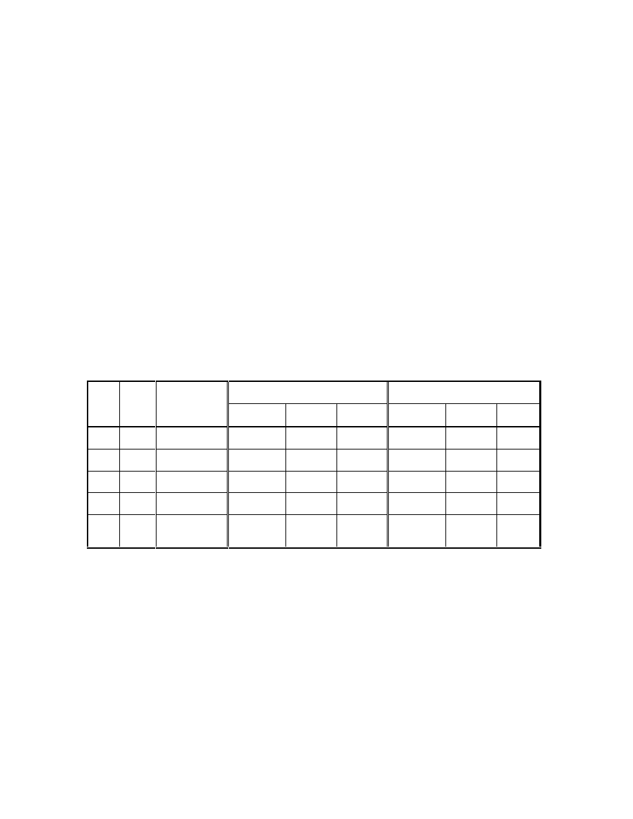
Table 1. Comparison of computational differences between the PCG2 and LMG solvers for

several different ground-water flow problems. Unless otherwise indicated, DAMP=1.0
and ICG=0 for all simulations. [SS, steady-state; TR, transient; L, linear; NL, nonlinear;
#, number; MB, megabyte]

PCG2

LMG

Prob-

lem

Type

# of Nodes

(# of layers,

# of rows,

# of columns)

CPU Time

(seconds)

Memory

(Mb)

# of

Iterations

CPU Time

(seconds)

Memory

(Mb)

# of

Cycles

1

SS

NL

1,728,000

(60, 240, 120)

3,082

121

565

1,761

1

1,352

940

1

966

40

1

24

2

SS

L

1,050,000

(1, 1500, 700)

5,243

50

2465

205

340

9

3

TR
NL

147,440

(4, 190, 194)

852

14

4328

631

72

175

4

SS

L

465,600

(15, 194, 160)

942

47

1864

50

151

9

5

SS

NL

74,817

(3, 163, 153)

654

8

3718

2

108

3

54

4

59

2

29

3

29

4

29

2

46

3

25

4

27

1

ICG=1

2

DAMP=0.50

3

DAMP=-1 (Adaptive damping using Cooley’s method)

4

DAMP=-2 (Adaptive damping using the relative reduced residual method)

Problem 1 is a very large, three-dimensional model. The variance of the hydraulic

conductivity field is approximately 2.0 (Sanford, W.E., U.S. Geological Survey, written
communication, 2000). The LMG Package uses a large amount of memory to solve this
problem, and the ICG option is helpful in reducing the CPU time.

Problem 2 is a large, two-dimensional model with a very complicated hydraulic

conductivity field (Konikow, L., and Hornberger, G., U.S. Geological Survey, written
communication, 2000). The LMG Package is very effective for this problem, reducing
execution time by a factor of 25, while using substantially more memory.

17

Problem 3 is a moderately sized, transient model (Roberts, C.F., U.S. Geological

Survey, written communication, 2001). The CPU time of both solvers is similar for this
problem. This is primarily because the solution at the current time step is used as the
initial head for the next time step, and in this case, the initial head approximation is very
close to the converged solution, so both solvers perform well.

Problem 4 is a large, three-dimensional model with a complex heterogeneous

hydraulic-conductivity field (O’Brien, G.M. and D’Agnese, F.A., U.S. Geological
Survey, written communication, 2000). As with problem 2, which also had a complex
heterogeneous field, the LMG Package performs very successfully for this problem.

Problem 5 is a moderately sized three-dimensional problem with very strong

nonlinearites resulting from evaportranspiration and a hydraulic conductivity field that is
also fairly complex (D’Agnese and others, 1998, and Tiedeman, C.R., U.S. Geological
Survey, written communication, 2000). The adaptive damping strategies are very
effective for this problem and reduce the number of cycles required for convergence.

The above results indicate that the LMG Package can substantially reduce the

CPU time compared to the PCG2 Package, particularly for problems involving complex
hydraulic-conductivity fields.

18

Compatibility, Portability and Memory Requirements

Compatibility and Portability

The LMG Package and the AMG solver are written in standard FORTRAN 77.

Subroutine CTIME is machine independent as distributed but can be modified as needed
for a given computer platform to calculate the computational times for various parts of
the algorithm. As distributed, CTIME is simply a dummy routine, and the values for
times printed when IOUTAMG = 2 or 3 (see Input Instructions) will always equal zero.
Most users don’t need internal timing information and will not need to change CTIME.
For users interested in investigating internal execution times, CTIME is distributed with
commented lines that correspond to the intrinsic timing functions for several platforms.
To calculate the computational times, the user needs to “uncomment” the section that
corresponds to the appropriate platform or use the intrinsic timing function for their
compiler, and recompile the program. However CTIME is handled, it will not affect the
performance of the AMG solver.

Memory Requirements

The LMG package uses a large amount of memory in the MODFLOW-2000 Z

and IX arrays. The AMG1R5 code is written in FORTRAN 77 instead of FORTRAN 90,
so three variables, STOR1, STOR2, and STOR3, are used to allocate memory for the
arrays required by the AMG routine. The nature of the algebraic multigrid algorithm is
such that the memory requirements cannot be determined beforehand. Nevertheless,
reasonable estimates based on the number of nodes (NODES) and the number of non-
zero elements in the coefficient matrix (NNA) can be used to allocate memory. The
formulas for array dimensions shown in table 2 are based on recommendations from the
authors of the AMG1R5 routine.

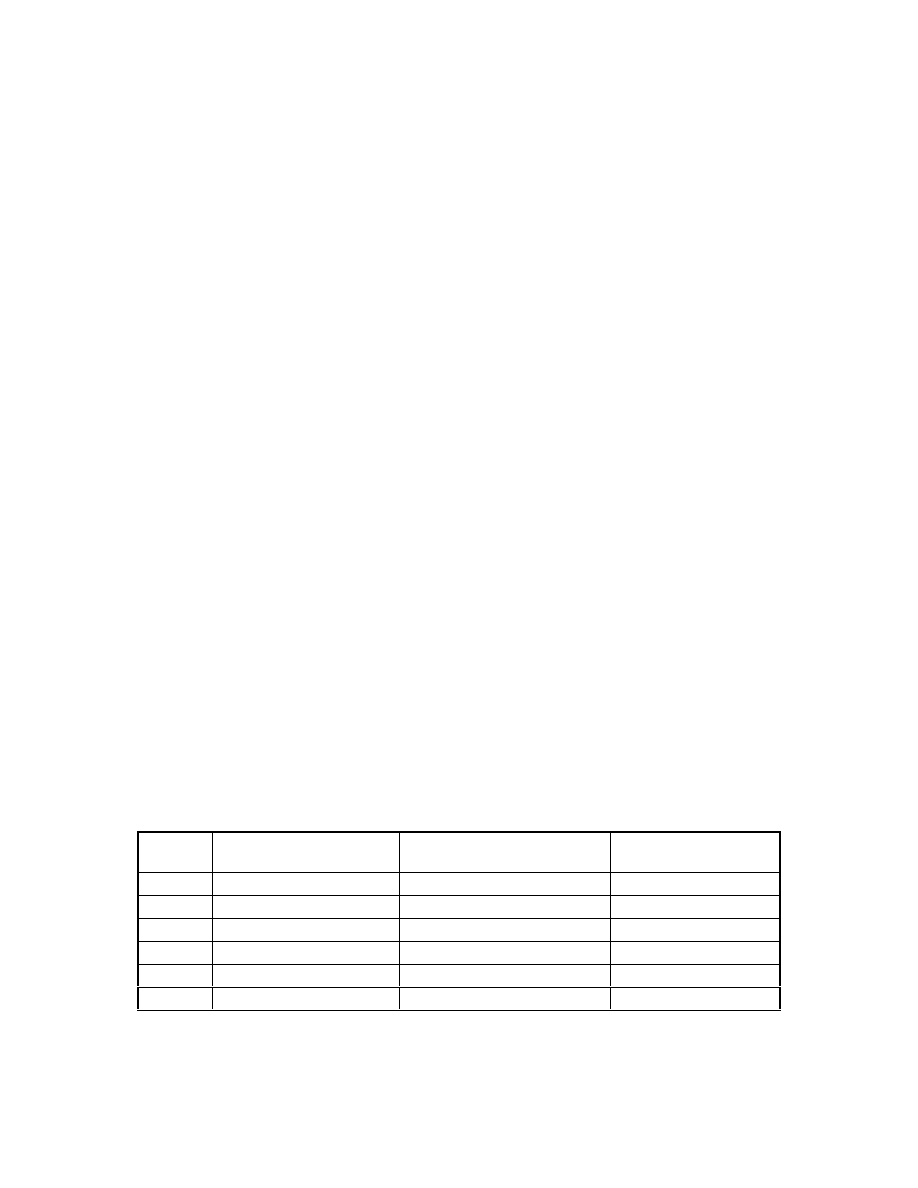
Table 2. Arrays used in AMG1R5, their dimensions, the user-defined variables that control the

storage allocated for the arrays, values recommended by Ruge and others (1990), and the
global storage arrays in MODFLOW-2000 in which the AMG1R5 arrays are stored.
[NODES, number of nodes in the grid; NNA, number of non-zero elements in the
coefficient matrix.]

Array

name

Dimension

User-Defined Variable and

Recommended Value

Global Storage Array

A

STOR1*NNA + 5*NODES

STOR1=3.0

Z

JA

STOR1*NNA + 5*NODES

STOR1=3.0

IX

IA

STOR2*NODES

STOR2=2.2

IX

U

STOR2*NODES

STOR2=2.2

Z

1

FRHS

STOR2*NODES

STOR2=2.2

Z

IG

STOR3*NODES

STOR3=5.4

IX

1

The array FHRS in the LMG package corresponds to the array F in the AMG1R5.

19

For most problems, the recommended values of STOR1, STOR2, and STOR3 are

adequate. However, if memory usage is a problem, the user can adjust the storage values
as necessary. The solver will stop and report an error if the storage space allocated for a
array is insufficient. In such cases, the variable controlling the storage for that array needs
to be increased.

20

Input Instructions and Sample Data Inputs

Input Instructions

The LMG Package reads its input data from the file indicated in the Name file as

described by Harbaugh and others (2000, p. 7, 43) using File Type LMG. Input for the
LMG Package is defined using two numbered items. Each item consists of several
parameters that are specified in one record and are read free format.

1.

STOR1

STOR2

STOR3

ICG

2.

MXITER MXCYC

BCLOSE

DAMP

IOUTAMG

Item 3 is read if

DAMP

= -2

3.

DUP

DLOW

STOR1 is a variable controlling the amount of storage allocated in the Z array for the

array A and the amount of storage allocated in the IX array for the array JA. For
most problems, a value of 3.0 should be adequate (table 2).

STOR2 is a variable controlling the amount of storage allocated in the Z array for the

arrays U and FRHS, and the amount of storage allocated in the IX array for the
array IA. For most problems, a value of 2.2 should be adequate (table 2).

STOR3 is a variable controlling the amount of storage allocated in the IX array for the

array IG. For most problems, a value of 5.4 should be adequate (table 2).

ICG is a variable controlling whether or not conjugate gradient iterations are used at the

end of each multigrid cycle. A value of 1 indicates that conjugate gradient
iterations will be performed, while a value of 0 indicates no conjugate gradient
iterations will be performed. All other values are automatically reset to 0. For
some problems, using conjugate gradient iterations can improve convergence,
but it will increase the memory used by the solver.

MXITER is the maximum number of iterations – that is, calls to the AMG solver. For

linear problems, MXITER can be set equal to 2. For nonlinear problems,
MXITER generally needs to be larger, but rarely more than 50.

MXCYC is the maximum number of cycles allowed per call to the solver. This is similar

to the variable ITER1 in PCG2 (Hill, 1990, p. 13). A value of 50 is suggested.
For some nonlinear problems, however, faster convergence may be achieved by
reducing MXCYC and increasing MXITER.

BCLOSE is the budget closure criterion for the scaled L

2

norm of the matrix equations

(eq. 3). A value similar to RCLOSE of PCG2 (Hill, 1990, p. 12-14) should be
used. If the global budget error is too large, decrease BCLOSE by one order of
magnitude to reduce the global budget error by about one order of magnitude.
This approximation can be used to adjust BCLOSE until a satisfactory solution is
attained. See the sections on Convergence Criterion and Tips for Achieving
Convergence for more information.

21

DAMP is a damping/accelerating parameter identical to ACCL of the DE4 (Harbaugh,

1995, p. 12) solver. Generally, a value of 1.0 is sufficient for most problems.
However, for nonlinear problems, values less than 1.0 may be necessary to
achieve convergence (see problem 5, table 2, for example).

DAMP>0 This value of DAMP is applied for all iterations.
DAMP=-1 Cooley’s method for adaptive damping is implemented.
DAMP=-2 The relative reduced residual method for adaptive damping is

implemented.

All other values of DAMP are automatically reset to 1.0 (no damping).

IOUTAMG is a flag that controls the information printed each time step from the solver

to the MODFLOW-2000 LIST output file (Harbaugh and others, 2000).
Diagnostic messages from the solver are sent to a temporary file called
“lmg_err.tmp” except if IOUTAMG=3, when they are printed along with the
other iteration information. The “lmg_err.tmp” file is deleted upon successful
termination of the solver. If the solver should fail, the output in this file may help
to identify solver problems. The possible values of IOUTAMG and the
information printed to the LIST file are as follows.

IOUTAMG=0 No printing from the solver to the LIST file.
IOUTAMG=1 Print scaling for residuals and residuals before and after cycling.
IOUTAMG=2 Print scaling for residuals, residuals before and after cycling, the

computer storage used, and the computation times if the CTIME
subroutine has been adapted to the computer operating system (see
Compatibility and Portability).

IOUTAMG=3 Print solver messages, scaling for residuals, residuals after each

cycle the computer storage used, and the computation times if the
CTIME subroutine has been adapted to the computer operating system
(see Compatibility and Portability).

DUP is the maximum value of DAMP that should be applied at any iteration. If the

adaptive scheme calculates a value of DAMP that is greater than DUP, DAMP
will be reset to DUP. A value of 1.0 is reasonable for most problems.

DLOW is the minimum value of DAMP that should be applied at any iteration. If the

adaptive scheme determines that the value of DAMP should be decreased, it will
calculate a new value of DAMP based on DLOW being the minimum (see eq. 7).
A value of 0.2 is reasonable for most problems.

22

Sample Data Inputs

Sample data inputs as listed below are for typical linear and nonlinear problems.

In these examples, the only differences are MXITER and DAMP. MXITER is typically 2
for linear problems. DAMP would generally be set to 1.0 for linear problems, but a value
less than 1.0 might be advantageous for nonlinear problems.

Example data set for a linear problem:

3.0 2.2 5.4 0
2 50 .001 1.0 1

Example data set for a nonlinear problem:

3.0 2.2 5.4 0
20 50 .001 .75 1

Example data set for a nonlinear problem with Cooley’s adaptive damping:

3.0 2.2 5.4 0
20 50 .001 -1.0 1

Example data set for a nonlinear problem with the relative reduced residual adaptive
damping scheme:

3.0 2.2 5.4 0
20 50 .001 -2.0 1
1.0 0.2

23

Brief Program Description

The LMG Package is composed of five modules, LMG1AL, LMG1RP,

LMG1AP, ADAMP1, and ADAMP2. The function of each module and the names of the
variables used are described in the following sections. Using the AMG solver also
requires the AMG1R5 subroutine by Ruge and others (1990), which contains
documentation within the source code, and the CTIME subroutine, which was discussed
under in the section “Compatibility and Portability.”

Narrative for Module LMG1AL

Module LMG1AP allocates space in the Z and IX arrays. This space is used by

the other modules in the LMG package and in the AMG routine. Storage is allocated for
the AMG arrays A, JA, IA, U, FRHS, and IG.

1. Print a message identifying the LMG Package.

2. Read values for STOR1, STOR2, STOR3, and ICG. Print values for STOR1, STOR2,

and STOR3. Check value ICG and set to 0 if necessary.

3. Calculate storage allocation based on STOR1, STOR2, STOR3, (see Memory

Requirements). Allocate space in the Z and IX arrays and set pointers for A, U,
FHRS, IA, JA, and IG.

4. Calculate and print space used in the Z and IX arrays

5. Return

List of Variables for Module LMG1AL

IAMG

Module Number of elements of the Z and IX arrays allocated for the

AMG solver.

ICG

Package Flag controlling the use of conjugate gradient iterations at the

end of each multigrid cycle.

IFREFM

Global

A parameter used to indicate if free format is used.

IN

Package Primary unit number from which input for this package will be

read.

IOUT

Global

Primary unit number for all printed output.

ISIZ1

Package STOR1*NNA+5*NODES

ISIZ2

Package STOR2*NODES

ISIZ3

Package STOR3*NODES

ISIZ4

Package Same as ISIZ2, unless ICG=1, then ISIZ2+NODES.

ISOLD

Module Value of ISUM upon entry into this module.

ISOLDI

Module Value of ISUMI upon entry into this module.

ISUM

Global

Element number of the lowest element in the Z array that has

24

not yet been allocated. When space is allocated to the Z

array, the size of the allocation is added to ISUM.

ISUM1

Module ISUM-1 or ISUMI-1

ISUMI

Global

Same as ISUM, but for the IX array

LCA

Package Location in the Z array of the first element of the array A.

LCFRHS

Package Location in the Z array of the first element of the array FRHS.

LCIA

Package Location in the IX array of the first element of the array IA.

LCIG

Package Location in the IX array of the first element of the array IG.

LCJA

Package Location in the Z array of the first element of the array JA.

LCU1

Package Location in the Z array of the first element of the array U.

LENIX

Global

Number of elements in the IX array (static storage).

LENZ

Global

Number of elements in the Z array (static storage).

LINE

Module Character string used to read in data from the AMG input file.

NCL

Module Number nodes per row of the grid (NCOL*NLAY).

NCOL

Global

Number of columns in the grid.

NLAY

Global

Number of layers in the grid.

NNA

Module The number of non-zero elements in the coefficient matrix [A].

Calculated as NODES+2*(NCOL-1)*NRL+

2*(NROW-1)*NCL+2*(NLAY-1)*NRC.

NODES

Global

Number of nodes in the grid (NCOL*NROW*NLAY).

NRC

Module Number of nodes per layer of the grid (NROW*NCOL).

NRL

Module Number nodes per column of the grid (NROW*NLAY).

NROW

Global

Number of rows in the grid.

STOR1

Module Storage factor for arrays A and JA.

STOR2

Module Storage factor for arrays FRHS, IA, and U.

STOR3

Module Storage factor for array IG.

25

Narrative for Module LMG1RP

Module LMG1RP reads and prepares data for the LMG package. Variables to

control operation of the solver are read. MXITER is the number of calls to the solver,
MXCYC is the maximum number of cycles per call to the solver, BCLOSE is a closure
criterion, DAMP is a damping parameter, and IOUTAMG controls output from the
solver.

1. Initialize HCLOSE so the sensitivity process, if used, executes without errors.

2. Read MXITER, MXCYC, BCLOSE, DAMP, and IOUTAMG. Check value of

DAMP. If using adaptive damping, set IADAMP and read DUP and DLOW if
necessary.

3. Print MXITER, MXCYC, BCLOSE, ICG, DAMP, and IOUTAMG. Print IADAMP,

DUP, and DLOW if appropriate.

4. Set IOUTAMG to a value that AMG requires by adding 10 to the value specified in

the LMG Package input file.

5. Return

List of Variables for Module LMG1RP

BCLOSE

Package Budget closure criterion.

DAMP

Package Damping/accelerating parameter for head change at each

iteration.

DLOW

Package Minimum value of damping.

DUP

Package Maximum value of damping.

HCLOSE

Global

Dummy variable set to zero. Initialized here because if

sensitivities are calculated, it requires HCLOSE to be

initialized.

IADAMP

Package Flag used to determine if adaptive damping is being used.

ICG

Package Flag controlling the use of conjugate gradient iterations at the

end of each multigrid cycle.

IFREFM

Global

A parameter used to indicate if free format is being used.

IN

Package Primary unit number from which input for this package will be

read.

IOUT

Global

Primary unit number for all printed output.

IOUTAMG

Package Flag controlling the printing from the solver.

MXCYC

Package Maximum number of AMG cycles per call to the solver.

MXITER

Package Maximum number of calls to the solver.

26

Narrative for Module LMG1AP

Module LMG1AP sets up the matrix equations in a form that is compatible with

the AMG solver provided by the GMD. This routine is called each time a head or
sensitivity solution is needed.

1. Initialize variables and clear arrays.

2. Loop through all nodes in the grid and set up coefficients of the matrix equations and

accumulate the L

2

norm of the current residual vector. This loop structure is identical

to that of subroutine PCG2AP of the PCG2 (Hill, 1990, p. 31-32) solver.

3. Reset the coefficients of the matrix equations such that the diagonal elements are

positive and the off-diagonal elements are negative. Set the diagonal to 1.0 and set
FRHS to HNEW for inactive cells or constant-head cells. Accumulate the average
absolute value of the FRHS vector for active cells and the maximum value of the
FRHS vector for all cells.

4. Use a skyline type storage to store the coefficients of the conductance matrix in a

single vector (A), with pointers to the diagonal (IA) and off diagonals (JA). For each
row in the matrix, start at the diagonal, then pick up non-zero elements moving from
left to right (but skipping the diagonal). Store initial value in vector U.

5. Set the dimensions for the variables used by the AMG solver. The extra storage is

used by the solver as workspace. Set variables for solver control.

6. Control printing from the solver based on the value of IOUTAMG. A temporary file

is opened for printing solver messages if IOUTAMG is < 13. The user inputs a value
of 3 for IOUTAMG, but 10 was added to this value to maintain compatibility the
AMG1R5 code.

7. Scale the L

2

norm closure criterion by the average absolute value and the maximum

value of FRHS. Print scaled values. Check convergence. If converged, close
temporary file (if necessary) and return.

8. Set up default values for the AMG solver. Call the AMG1R5 subroutine.

9. Check for solver errors. If there are errors, print identifying messages and stop. If the

solver executed successfully, apply damping strategy, then close temporary output
file (if necessary).

10. Return

27

List of Variables for Module LMG1AP

A

Module DIMENSION(ISIZ1), double precision array containing the

coefficient matrix [A].

BCLOSE

Package Budget closure criterion.

CC

Global

Dimension(NCOL,NROW,NLAY), conductances along

columns.

CR

Global

Dimension(NCOL,NROW,NLAY), conductances along rows.

CV

Global

Dimension(NCOL,NROW,NLAY), conductances between

layers.

DAMP

Package Damping/accelerating parameter for head change at each

iteration.

DDAMP

Package Double precision form of DAMP.

DHMAX

Package Head change for current iteration that is maximum absolute

value.

DLOW

Package Minimum value of damping.

DONE

Module Double precision variable containing a value of unity.

DUP

Package Maximum value of damping.

DZERO

Module Double precision variable containing a value of zero.

ECG1

Module Double precision variable equal to 0.D0.

ECG2

Module Double precision variable equal to 0.25D0.

EPS

Module Double precision BCLOSE*FBAR/FMAX used for AMG

scaled residual closure criterion.

EWT2

Module Double precision variable equal to 0.35D0.

FBAR

Module Double precision average of ABS(FRHS) for active nodes.

FMAX

Module Double precision maximum ABS(FRHS) for active nodes.

FRHS

Module DIMENSION(ISIZ2), double precision form of -RHS.

HCOF

Global

DIMENSION(NCOL,NROW,NLAY), coefficient of head in the

finite-difference equations.

HNEW

Global

DIMENSION(NCOL,NROW,NLAY), most recent estimate of

head in each cell.

IA

Module DIMENSION(ISIZ2), array containing the location of the

diagonal element in the coefficient matrix [A].

IADAMP

Package Flag used to determine if adaptive damping is being used.

IBOUND

Global

DIMENSION(NCOL,NROW,NLAY), status of each cell:

< 0 – constant-head cell

= 0 – no-flow cell

> 0 – variable head cell

ICG

Package Flag controlling the use of conjugate gradient iterations at the

end of each multigrid cycle.

ICNVG

Global

Flag that is set to one when convergence has occurred.

IFIRST

Package Integer variable set equal to 10 which allows the current head to

be used as the initial solution within the AMG1R5.

IG

Module DIMENSION(ISIZ3), work array used by the AMG solver.

ILMGTMP

Module Primary unit number to which messages from the solver will be

printed if IOUTAMG = 0, 1, or 2.

28

IOUT

Global

Primary unit number for all printed output.

IOUTAMG

Package Flag controlling the printing from the AMG solver.

ISIZ1

Package STOR1*NNA+5*NODES

ISIZ2

Package STOR2*NODES

ISIZ3

Package STOR3*NODES

ISIZ4

Package Same as ISIZ2, unless ICG=1, then ISIZ2+NODES.

ISWTCH

Package Integer variable set equal to 4 so that all modules of the

AMG1R5 are called.

IZERO

Module Integer variable containing zero.

JA

Module DIMENSION(ISIZ1), array containing the location of the off-

diagonal elements of the coefficient matrix [A].

KITER

Global

Counts the number of calls to the solver.

LEVELX

Package Integer variable set equal to 0 so that a standard value is used

by the AMG1R5.

MADAPT

Package Integer variable set equal to 0 so that a standard value is used

by the AMG1R5.

MATRIX

Package Integer variable set equal to 22 which defines properties of the

matrix for the AMG1R5.

MXCYC

Package Maximum number of AMG cycles per call to the solver.

MXITER

Package Maximum number of calls to the solver.

N

Module Cell index.

NA

Module Index for array A.

NCD

Module One-dimensional subscript of conductance to the adjacent cell,

which is in the previous column.

NCF

Module One-dimensional subscript of conductance to the adjacent cell,

which is in the next column.

NCL

Module One-dimensional subscript of the cell index of the adjacent cell

which is in the previous column.

NCN

Module One-dimensional subscript of the cell index of the adjacent cell

which is in the next column.

NCOL

Global

Number of columns in the grid.

NCOUNT

Module Number of active nodes.

NCYC

Package Integer variable that controls the number and type of cycles

used by the AMG1R5.

NDF

Package Dimensioning for FRHS. Same as ISIZ4.

NDA

Package Dimensioning for A. Same as ISIZ1.

NDIA

Package Dimensioning for IA. Same as ISIZ2.

NDIG

Package Dimensioning for IG. Same as ISIZ3.

NDJA

Package Dimensioning for JA. Same as ISIZ1.

NDU

Package Dimensioning for U. Same as ISIZ4.

NJ

Module Index for array JA.

NLAY

Global

Number of layers in the grid.

NLL

Module One-dimensional subscript of the cell index of the adjacent cell,

which is in the previous layer.

NLN

Module One-dimensional subscript of the cell index of the adjacent cell,

which is in the next layer.

29

NLS

Module One-dimensional subscript of conductance to the adjacent cell,

which is in the next layer.

NLZ

Module One-dimensional subscript of conductance to the adjacent cell,

which is in the previous layer.

NNU

Package Number of unknowns. Same as NODES.

NODES

Global

Number of nodes in the grid (NCOL*NROW*NLAY).

NRB

Module One-dimensional subscript of conductance to the adjacent cell,

which is in the previous row.

NRC

Module Number of nodes per layer of the grid (NROW*NCOL).

NRD

Package Integer variable set equal to 0 so that a standard value is used

by the AMG1R5.

NRH

Module One-dimensional subscript of conductance to the adjacent cell,

which is in the next row.

NRL

Module One-dimensional subscript of the cell index of the adjacent cell,

which is in the previous row.

NRN

Module One-dimensional subscript of the cell index of the adjacent cell,

which is in the next row.

NROW

Global

Number of rows in the grid.

NRU

Package Integer variable set equal to 0 so that a standard value is used

by the AMG1R5.

NSOLCO

Package Integer variable set equal to 2 so that the AMG1R5 uses a direct

solver on the coarsest grid.

NTR

Package Integer variable set equal to 0 so that a standard value is used

by the AMG1R5.

NWT

Package Integer variable set equal to 2 which is a standard value for the

AMG1R5.

RHS

Global

DIMENSION(NCOL,NROW,NLAY) right-hand side of the

finite-difference equations.

RSQ

Module Double precision variable containing the current sum of squared

residuals of the finite-difference equations.

TMP

Module Temporary variable used when finding DHMAX.

U

Module DIMENSION(ISIZ2) initial value upon entry to AMG solver

and solution vector upon exit from AMG solver.

30

Narrative for Module ADAMP1

Module ADAMP1 changes the value of the damping parameter, DAMP, based on

the maximum head change from the previous and current iterations. The strategy used is
that proposed by Cooley (1983) and later modified by Huyakorn and others (1986).

1. Initialize S and calculate according to equation 4, if not on the first iteration.

2. Based on the value of S, apply damping according to equation 5. Values greater than

or equal to -1 indicate the solution is progressing adequately and the damping is not
very aggressive. The converse is true for values of S that are less than -1.

3. Return

List of Variables for Module ADAMP1

DHMAX

Package Head change for current iteration that is maximum absolute

value.

DHOLD

Module Value of DHMAX at the previous iteration.

KITER

Global

Counts the number of calls to the solver.

S

Module Fractional change in the maximum head change, scaled by the

damping parameter. Calculated as DHMAX/DHOLD/WK.

WK

Package Same as DDAMP.

Narrative for Module ADAMP2

Module ADAMP2 changes the value of the damping parameter, DAMP, based on

the L

2

norm of the residuals from the current and two prior iterations. The strategy used is

empirical and based on damping more aggressively if the residuals are not lowered
sufficiently or if they are oscillating.

1. Calculate current residual and initialize variables for the first iteration.

2. Calculate the relative reduction in the L

2

norm scaled by the applied damping (RRED,

see equation 6). If RRED is greater than 50 percent then moderate damping is applied
with a value of DDAMP equal to RRED, but not greater than DUP. Thus, for larger
RRED, the solution is progressing adequately and the value of DDAMP should
approach 1.0 or DUP. The converse is true for RRED less than 50 percent. The
damping is more aggressive for poorer reductions with a minimum value of DLOW.
Note that the maximum value of DDAMP for this case will be DLOW + 0.3 (see
equation 7).

31

3. Calculate the relative change in the L

2

norm between the current residual and the

residual from two iterations ago (OSTERM). If they are within 10 percent of each
other, then the solution is oscillating. Check to make sure DDAMP does not exceed
DUP. If the solution is oscillating and the current value of DDAMP is within 1
percent of the damping that was applied two iterations ago (DAMP3), then the
solution will continue to oscillate in this area. In this case, generate a random value of
DDAMP between 0 and 1.5 to try and perturb the solution out of this area.

4. Store the values of the L

2

norm and damping for the next iteration.

5. Return.

List of Variables for Module ADAMP2

DAMP

Package Damping/accelerating parameter for head change at each

iteration. Current value of DAMP upon entry. Previous value

of damping upon exit.

DAMP3

Module Value of DDAMP two iterations ago.

DDAMP

Package Double precision form of DAMP.

DLOW

Package Minimum value of damping.

DUP

Package Maximum value of damping.

RRED

Module Relative reduction of the residuals scaled by the damping

parameter. Calculated as (RSQ2-RSQ1)/RSQ2/DDAMP.

ICONST

Module Integer used for random number generation. Equals 49297.

IMULT

Module Integer used for random number generation. Equals 9301.

IPER

Module Integer used for random number generation. Equals 233280.

KITER

Global

Counts the number of calls to the solver.

NRAN

Module Integer used in generating a random number.

OSCIL

Module Logical variable to flag if the solution is oscillating.

OSTERM

Module Variable used to determine if the solution is oscillating by

measuring relative difference in residuals. Calculated as

(RSQ3-RSQ1)/RSQ3.

QRAND

Module Quick random number generated uniformly between 0 and 1.

RSQ1

Package Double precision variable containing the current sum of squared

residuals of the finite-difference equations upon entry.

Square root of the sum of squared residuals value upon exit.

RSQ2

Module Double precision variable containing the value of RSQ1 at the

previous iteration.

RSQ3

Module Double precision variable containing the value of RSQ2 at the

previous iteration (the same as RSQ1 two iterations ago).

32

References

Briggs, W.L., Henson, V.E., and McCormick, S.F., 2000, A multigrid tutorial: 2nd ed.:

Philadelphia, Society for Industrial and Applied Mathematics, 193 p.

Cleary, A.J., Falgout, R.D., Henson, V.E., Jones, J.E., Manteuffel, T.A., McCormick,

S.F., Miranda, G.N., and Ruge, J.W., 2000, Robustness and scalability of
algebraic multigrid: SIAM Journal on Scientific Computing, v. 21, no. 5, p.
1886-1908.

Cooley, R. L., 1983, Some new procedures for numerical-solution of variably saturated

flow problems: Water Resources Research, v. 19, no. 5, p. 1271-1285.

D’Angese, F.A., Faunt, C.C., Turner, A.K., and Hill, M.C., 1998, Hydrogeologic

evaluation and numerical simulation of the Death Valley regional ground-water
flow system, Nevada and California: U.S. Geological Survey Water-Resources
Investigation Report 96-4300, 124 p.

Demmel, J.W., 1997, Applied Numerical linear algebra: Philadelphia, Society for

Industrial and Applied Mathematics, 419 p.

Harbaugh, A.W., 1995, Direct Solution Package Based on Alternating Diagonal Ordering

for the U.S. Geological Survey Modular Finite-Difference Ground-Water Flow
Model: U.S. Geological Survey Open-File Report 95-288, 46 p.

Harbaugh, A.W., Banta, E.R., Hill, M.C., and McDonald, M.G., 2000, MODFLOW-

2000, The U.S. Geological Survey modular ground-water model – User guide to
modularization concepts and the ground-water flow process: U.S. Geological
Survey Open-File Report 00-92, 121 p.

Hill, M.C., 1990, Preconditioned Conjugate-Gradient 2 (PCG2), A computer program for

solving ground-water flow equations: U.S. Geological Survey Water-Resources
Investigations Report 90-4048, 43 p.

Hill, M.C., Banta, E.R., Harbaugh, A.W., and Anderman, E.R., 2000, MODFLOW-2000,

The U.S. Geological Survey modular ground-water model – User guide to the
observation, sensitivity, and parameter-estimation processes and three post-
processing programs: U.S. Geological Survey Open-File Report 00-184, 209 p.

Huyakorn, P.S., Springer, E.P., Guvanasen, V., and Wadsworth, T.D., 1986, A 3-

dimensional finite-element model for simulating water-flow in variably saturated
porous-media: Water Resources Research, v. 22, no. 13, p. 1790-1808.

Kipp, K.L., Konikow, L.F., and Hornberger, G.Z., 1998, An implicit dispersive transport

algorithm for the U.S Geological Survey MOC3D solute-transport model: U.S.
Geological Survey Water-Resources Investigations Report 98-4234, 54 p.

McDonald, M.G., and A.W. Harbaugh, 1988, A modular three-dimensional finite-

difference ground-water flow model: U.S. Geological Survey Techniques of
Water-Resources Investigations, Book 6, Chapter A1, 548 p.

Paniconi, C., and Putti, M., 1994, A comparison of Picard and Newton iteration in the

numerical-solution of multidimensional variably saturated flow problems: Water
Resources Research, v. 30, no. 12, p. 3357-3374.

Ruge, J, K., and Stüben, K., 1987, Algebraic Multigrid, in McCormick, S.F. ed.,

Multigrid Methods: Philadelphia, Society for Industrial and Applied
Mathematics, p. 73-130.

33

Ruge, J., Stüben, K., and Hempel, R., 1990, AMG1R5, accessed March 12, 2001 at URL

http://www.mgnet.org/mgnet/Codes/gmd/amg.tgz.

Stüben, K., 1999, Algebraic multigrid (AMG) – An introduction with applications:

Gesellschaft für Mathematik und Datenverarbeitung mbH (GMD) Report 70, 127
p.

______2001, A review of algebraic multigrid: Journal of Computational and Applied

Mathematics, v. 128, no. 1-2, p. 281-309.

Wagner, C., Kinzelback, W., and Wittum, G., 1997, Schur-complement multigrid – A

robust method for groundwater flow and transport problems: Numerische
Mathematik, v. 75, no. 4, p. 523-545.

34