
VHDL Tutorial
Peter J. Ashenden
EDA C
ONSULTANT
, A
SHENDEN
D
ESIGNS
P
TY
. L
TD
.
www.ashenden.com.au
© 2004 by Elsevier Science (USA)
All rights reserved


1
1
Introduction
The purpose of this tutorial is to describe the modeling language VHDL. VHDL in-
cludes facilities for describing logical structure and function of digital systems at a
number of levels of abstraction, from system level down to the gate level. It is intend-
ed, among other things, as a modeling language for specification and simulation. We
can also use it for hardware synthesis if we restrict ourselves to a subset that can be
automatically translated into hardware.
VHDL arose out of the United States government’s Very High Speed Integrated
Circuits (VHSIC) program. In the course of this program, it became clear that there
was a need for a standard language for describing the structure and function of inte-
grated circuits (ICs). Hence the VHSIC Hardware Description Language (VHDL) was
developed. It was subsequently developed further under the auspices of the Institute
of Electrical and Electronic Engineers (IEEE) and adopted in the form of the IEEE Stan-
dard 1076, Standard VHDL Language Reference Manual, in 1987. This first standard
version of the language is often referred to as VHDL-87.
Like all IEEE standards, the VHDL standard is subject to review at least every five
years. Comments and suggestions from users of the 1987 standard were analyzed by
the IEEE working group responsible for VHDL, and in 1992 a revised version of the
standard was proposed. This was eventually adopted in 1993, giving us VHDL-93. A
further round of revision of the standard was started in 1998. That process was com-
pleted in 2001, giving us the current version of the language, VHDL-2002.
This tutorial describes language features that are common to all versions of the
language. They are expressed using the syntax of VHDL-93 and subsequent versions.
There are some aspects of syntax that are incompatible with the original VHDL-87 ver-
sion. However, most tools now support at least VHDL-93, so syntactic differences
should not cause problems.
The tutorial does not comprehensively cover the language. Instead, it introduces
the basic language features that are needed to get started in modeling relatively simple
digital systems. For a full coverage, the reader is referred to The Designer’s Guide to
VHDL, 2nd Edition, by Peter J. Ashenden, published by Morgan Kaufman Publishers
(ISBN 1-55860-674-2).


3
2
Fundamental Concepts
2.1
Modeling Digital Systems
The term digital systems encompasses a range of systems from low-level components
to complete system-on-a-chip and board-level designs. If we are to encompass this
range of views of digital systems, we must recognize the complexity with which we
are dealing. It is not humanly possible to comprehend such complex systems in their
entirety. We need to find methods of dealing with the complexity, so that we can,
with some degree of confidence, design components and systems that meet their re-
quirements.
The most important way of meeting this challenge is to adopt a systematic meth-
odology of design. If we start with a requirements document for the system, we can
design an abstract structure that meets the requirements. We can then decompose
this structure into a collection of components that interact to perform the same func-
tion. Each of these components can in turn be decomposed until we get to a level
where we have some ready-made, primitive components that perform a required
function. The result of this process is a hierarchically composed system, built from
the primitive elements.
The advantage of this methodology is that each subsystem can be designed inde-
pendently of others. When we use a subsystem, we can think of it as an abstraction
rather than having to consider its detailed composition. So at any particular stage in
the design process, we only need to pay attention to the small amount of information
relevant to the current focus of design. We are saved from being overwhelmed by
masses of detail.
We use the term model to mean our understanding of a system. The model rep-
resents that information which is relevant and abstracts away from irrelevant detail.
The implication of this is that there may be several models of the same system, since
different information is relevant in different contexts. One kind of model might con-
centrate on representing the function of the system, whereas another kind might rep-
resent the way in which the system is composed of subsystems.
There are a number of important motivations for formalizing this idea of a model,
including
• expressing system requirements in a complete and unambiguous way
• documenting the functionality of a system
• testing a design to verify that it performs correctly
4
Fundamental Concepts
• formally verifying properties of a design
• synthesizing an implementation in a target technology (e.g., ASIC or FPGA)
The unifying factor is that we want to achieve maximum reliability in the design
process for minimum cost and design time. We need to ensure that requirements are
clearly specified and understood, that subsystems are used correctly and that designs
meet the requirements. A major contributor to excessive cost is having to revise a
design after manufacture to correct errors. By avoiding errors, and by providing better
tools for the design process, costs and delays can be contained.
2.2
VHDL Modeling Concepts
In this section, we look at the basic VHDL concepts for behavioral and structural mod-
eling. This will provide a feel for VHDL and a basis from which to work in later chap-
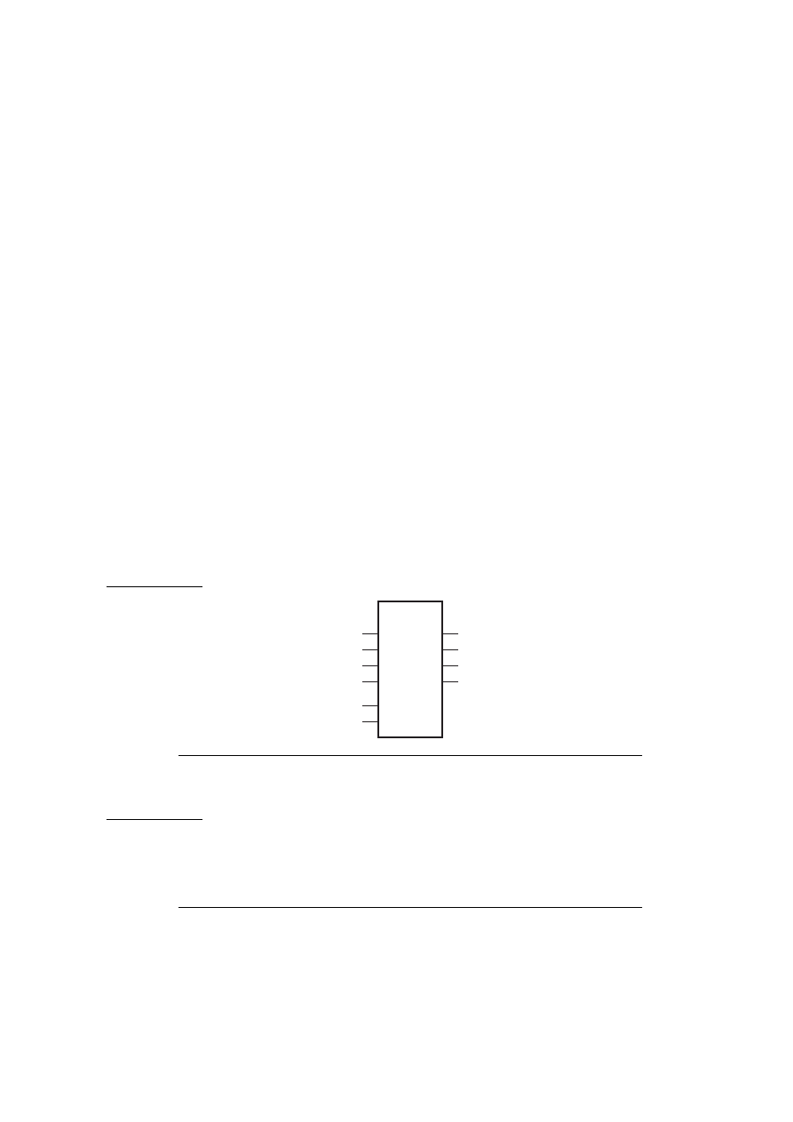
ters. As an example, we look at ways of describing a four-bit register, shown in
Figure 2-1.
Using VHDL terminology, we call the module
reg4
a design entity, and the inputs
and outputs are ports. Figure 2-2 shows a VHDL description of the interface to this
entity. This is an example of an entity declaration. It introduces a name for the entity
and lists the input and output ports, specifying that they carry bit values (‘0’ or ‘1’) into
and out of the entity. From this we see that an entity declaration describes the external
view of the entity.
FIGURE 2-1
A four-bit register module. The register is named
reg4
and has six inputs,
d0
,
d1
,
d2
,
d3
,
en
and
clk
, and
four outputs,
q0
,
q1
,
q2
and
q3
.
FIGURE 2-2
entity reg4 is
port ( d0, d1, d2, d3, en, clk : in bit;
q0, q1, q2, q3 : out bit );
end entity reg4;
A VHDL entity description of a four-bit register.
reg4
d0
q0
q1
q2
q3
d1
d2
d3
en
clk

VHDL Modeling Concepts
5
Elements of Behavior
In VHDL, a description of the internal implementation of an entity is called an archi-
tecture body of the entity. There may be a number of different architecture bodies of
the one interface to an entity, corresponding to alternative implementations that per-
form the same function. We can write a behavioral architecture body of an entity,
which describes the function in an abstract way. Such an architecture body includes
only process statements, which are collections of actions to be executed in sequence.
These actions are called sequential statements and are much like the kinds of state-
ments we see in a conventional programming language. The types of actions that can
be performed include evaluating expressions, assigning values to variables, condition-
al execution, repeated execution and subprogram calls. In addition, there is a sequen-
tial statement that is unique to hardware modeling languages, the signal assignment
statement. This is similar to variable assignment, except that it causes the value on a
signal to be updated at some future time.
To illustrate these ideas, let us look at a behavioral architecture body for the
reg4
entity, shown in Figure 2-3. In this architecture body, the part after the first
begin
key-
word includes one process statement, which describes how the register behaves. It
starts with the process name,
storage
, and finishes with the keywords
end process
.
FIGURE 2-3
architecture behav of reg4 is
begin
storage : process is
variable stored_d0, stored_d1, stored_d2, stored_d3 : bit;
begin
wait until clk = '1';
if en = '1' then
stored_d0 := d0;
stored_d1 := d1;
stored_d2 := d2;
stored_d3 := d3;
end if;
q0 <= stored_d0 after 5 ns;
q1 <= stored_d1 after 5 ns;
q2 <= stored_d2 after 5 ns;
q3 <= stored_d3 after 5 ns;
end process storage;
end architecture behav;
A behavioral architecture body of the
reg4
entity.
The process statement defines a sequence of actions that are to take place when
the system is simulated. These actions control how the values on the entity’s ports
change over time; that is, they control the behavior of the entity. This process can
modify the values of the entity’s ports using signal assignment statements.
The way this process works is as follows. When the simulation is started, the sig-
nal values are set to ‘0’, and the process is activated. The process’s variables (listed

6
Fundamental Concepts
after the keyword
variable
) are initialized to ‘0’, then the statements are executed in
order. The first statement is a wait statement that causes the process to suspend. Whil
the process is suspended, it is sensitive to the
clk
signal. When clk changes value to
‘1’, the process resumes.
The next statement is a condition that tests whether the
en
signal is ‘1’. If it is, the
statements between the keywords
then
and
end if
are executed, updating the pro-
cess’s variables using the values on the input signals. After the conditional if state-
ment, there are four signal assignment statements that cause the output signals to be
updated 5 ns later.
When the process reaches the end of the list of statements, they are executed
again, starting from the keyword
begin
, and the cycle repeats. Notice that while the
process is suspended, the values in the process’s variables are not lost. This is how
the process can represent the state of a system.
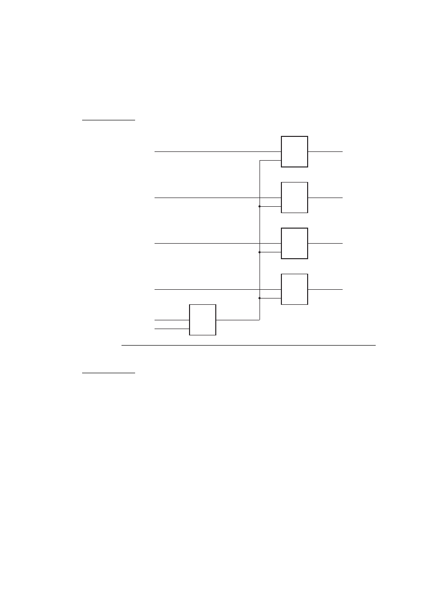
Elements of Structure
An architecture body that is composed only of interconnected subsystems is called a
structural architecture body. Figure 2-4 shows how the
reg4
entity might be com-
posed of D-flipflops. If we are to describe this in VHDL, we will need entity declara-
tions and architecture bodies for the subsystems, shown in Figure 2-5.
Figure 2-6 is a VHDL architecture body declaration that describes the structure
shown in Figure 2-4. The signal declaration, before the keyword
begin
, defines the
internal signals of the architecture. In this example, the signal
int_clk
is declared to
carry a bit value (‘0’ or ‘1’). In general, VHDL signals can be declared to carry arbi-
trarily complex values. Within the architecture body the ports of the entity are also
treated as signals.
In the second part of the architecture body, a number of component instances are
created, representing the subsystems from which the
reg4
entity is composed. Each
component instance is a copy of the entity representing the subsystem, using the cor-
responding
basic
architecture body. (The name
work
refers to the current working li-
brary, in which all of the entity and architecture body descriptions are assumed to be
held.)
The port map specifies the connection of the ports of each component instance
to signals within the enclosing architecture body. For example,
bit0
, an instance of
the
d_ff
entity, has its port
d
connected to the signal
d0
, its port
clk
connected to the
signal
int_clk
and its port
q
connected to the signal
q0
.
Test Benches
We often test a VHDL model using an enclosing model called a test bench. The name
comes from the analogy with a real hardware test bench, on which a device under
test is stimulated with signal generators and observed with signal probes. A VHDL
test bench consists of an architecture body containing an instance of the component
to be tested and processes that generate sequences of values on signals connected to
the component instance. The architecture body may also contain processes that test
that the component instance produces the expected values on its output signals. Al-
ternatively, we may use the monitoring facilities of a simulator to observe the outputs.
VHDL Modeling Concepts
7
FIGURE 2-4
A structural composition of the
reg4
entity.
FIGURE 2-5
entity d_ff is
port ( d, clk : in bit; q : out bit );
end d_ff;
architecture basic of d_ff is
begin
ff_behavior : process is
begin
wait until clk = '1';
q <= d after 2 ns;
end process ff_behavior;
end architecture basic;
––––––––––––––––––––––––––––––––––––––––––––––––––––
entity and2 is
port ( a, b : in bit; y : out bit );
end and2;
d_ff
d
bit0
q
clk
d_ff
d
bit1
q
clk
d_ff
d
bit2
q
clk
d_ff
d
bit3
q
clk
and2
a
gate
y
b
q0
q1
q2
q3
clk
en
d0
d1
d2
d3
int_clk

8
Fundamental Concepts
architecture basic of and2 is
begin
and2_behavior : process is
begin
y <= a and b after 2 ns;
wait on a, b;
end process and2_behavior;
end architecture basic;
Entity declarations and architecture bodies for D-flipflop and two-input and gate.
FIGURE 2-6
architecture struct of reg4 is
signal int_clk : bit;
begin
bit0 : entity work.d_ff(basic)
port map (d0, int_clk, q0);
bit1 : entity work.d_ff(basic)
port map (d1, int_clk, q1);
bit2 : entity work.d_ff(basic)
port map (d2, int_clk, q2);
bit3 : entity work.d_ff(basic)
port map (d3, int_clk, q3);
gate : entity work.and2(basic)
port map (en, clk, int_clk);
end architecture struct;
A VHDL structural architecture body of the
reg4
entity.
A test bench model for the behavioral implementation of the
reg4
register is
shown in Figure 2-7. The entity declaration has no port list, since the test bench is
entirely self-contained. The architecture body contains signals that are connected to
the input and output ports of the component instance
dut
, the device under test. The
process labeled
stimulus
provides a sequence of test values on the input signals by
performing signal assignment statements, interspersed with wait statements. We can
use a simulator to observe the values on the signals
q0
to
q3
to verify that the register
operates correctly. When all of the stimulus values have been applied, the stimulus
process waits indefinitely, thus completing the simulation.
FIGURE 2-7
entity test_bench is
end entity test_bench;
architecture test_reg4 of test_bench is
signal d0, d1, d2, d3, en, clk, q0, q1, q2, q3 : bit;
begin

VHDL Modeling Concepts
9
dut : entity work.reg4(behav)
port map ( d0, d1, d2, d3, en, clk, q0, q1, q2, q3 );
stimulus : process is
begin
d0 <= '1'; d1 <= '1'; d2 <= '1'; d3 <= '1';
en <= '0'; clk <= '0';
wait for 10 ns;
en <= '1'; wait for 10 ns;
clk = '1', '0' after 10 ns; wait for 20 ns;
d0 <= '0'; d1 <= '0'; d2 <= '0'; d3 <= '0';
en <= '0'; wait for 10 ns;
clk <= '1', '0' after 10 ns; wait for 20 ns;
…
wait;
end process stimulus;
end architecture test_reg4;
A VHDL test bench for the
reg4
register model.
Analysis, Elaboration and Execution
One of the main reasons for writing a model of a system is to enable us to simulate
it. This involves three stages: analysis, elaboration and execution. Analysis and elab-
oration are also required in preparation for other uses of the model, such as logic syn-
thesis.
In the first stage, analysis, the VHDL description of a system is checked for various
kinds of errors. Like most programming languages, VHDL has rigidly defined syntax
and semantics. The syntax is the set of grammatical rules that govern how a model
is written. The rules of semantics govern the meaning of a program. For example, it
makes sense to perform an addition operation on two numbers but not on two pro-
cesses.
During the analysis phase, the VHDL description is examined, and syntactic and
static semantic errors are located. The whole model of a system need not be analyzed
at once. Instead, it is possible to analyze design units, such as entity and architecture
body declarations, separately. If the analyzer finds no errors in a design unit, it creates
an intermediate representation of the unit and stores it in a library. The exact mech-
anism varies between VHDL tools.
The second stage in simulating a model, elaboration, is the act of working through
the design hierarchy and creating all of the objects defined in declarations. The ulti-
mate product of design elaboration is a collection of signals and processes, with each
process possibly containing variables. A model must be reducible to a collection of
signals and processes in order to simulate it.
The third stage of simulation is the execution of the model. The passage of time
is simulated in discrete steps, depending on when events occur. Hence the term dis-
crete event simulation is used. At some simulation time, a process may be stimulated
by changing the value on a signal to which it is sensitive. The process is resumed and
may schedule new values to be given to signals at some later simulated time. This is
called scheduling a transaction on that signal. If the new value is different from the

10
Fundamental Concepts
previous value on the signal, an event occurs, and other processes sensitive to the sig-
nal may be resumed.
The simulation starts with an initialization phase, followed by repetitive execu-
tion of a simulation cycle. During the initialization phase, each signal is given an ini-
tial value, depending on its type. The simulation time is set to zero, then each process
instance is activated and its sequential statements executed. Usually, a process will
include a signal assignment statement to schedule a transaction on a signal at some
later simulation time. Execution of a process continues until it reaches a wait state-
ment, which causes the process to be suspended.
During the simulation cycle, the simulation time is first advanced to the next time
at which a transaction on a signal has been scheduled. Second, all the transactions
scheduled for that time are performed. This may cause some events to occur on some
signals. Third, all processes that are sensitive to those events are resumed and are
allowed to continue until they reach a wait statement and suspend. Again, the pro-
cesses usually execute signal assignments to schedule further transactions on signals.
When all the processes have suspended again, the simulation cycle is repeated. When
the simulation gets to the stage where there are no further transactions scheduled, it
stops, since the simulation is then complete.

11
3
VHDL is Like a
Programming Language
3.1
Lexical Elements and Syntax
When we learn a new language, we need to learn how to write the basic elements,
such as numbers and identifiers. We also need to learn the syntax, that is, the gram-
mar rules governing how we form language constructs. We will briefly describe the
lexical elements and our notation for the grammar rules, and then start to introduce
langauge features.
VHDL uses characters in the ISO 8859 Latin-1 8-bit character set. This includes
uppercase and lowercase letters (including letters with diacritical marks, such as ‘à’,
‘ä’ and so forth), digits 0 to 9, punctuation and other special characters.
Comments
When we are writing a hardware model in VHDL, it is important to annotate the code
with comments. A VHDL model consists of a number of lines of text. A comment
can be added to a line by writing two dashes together, followed by the comment text.
For example:
… a line of VHDL description …
–– a descriptive comment
The comment extends from the two dashes to the end of the line and may include
any text we wish, since it is not formally part of the VHDL model. The code of a
model can include blank lines and lines that only contain comments, starting with two
dashes. We can write long comments on successive lines, each starting with two
dashes, for example:
–– The following code models
–– the control section of the system
… some VHDL code …
Identifiers
Identifiers are used to name items in a VHDL model. An identifier

12
VHDL is Like a Programming Language
• may only contain alphabetic letters (‘A’ to ‘Z’ and ‘a’ to ‘z’), decimal digits (‘0’
to ‘9’) and the underline character (‘_’);
• must start with an alphabetic letter;
• may not end with an underline character; and
• may not include two successive underline characters.
Case of letters is not significant. Some examples of valid basic identifiers are
A
X0
counter
Next_Value
generate_read_cycle
Some examples of invalid basic identifiers are
last@value
–– contains an illegal character for an identifier
5bit_counter
–– starts with a nonalphabetic character
_A0
–– starts with an underline
A0_
–– ends with an underline
clock__pulse
–– two successive underlines
Reserved Words
Some identifiers, called reserved words or keywords, are reserved for special use in
VHDL, so we cannot use them as identifiers for items we define. The full list of re-
served words is shown in Figure 3-1.
FIGURE 3-1
abs
access
after
alias
all
and
architecture
array
assert
attribute
begin
block
body
buffer
bus
case
component
configuration
constant
disconnect
downto
else
elsif
end
entity
exit
file
for
function
generate
generic
group
guarded
if
impure
in
inertial
inout
is
label
library
linkage
literal
loop
map
mod
nand
new
next
nor
not
null
of
on
open
or
others
out
package
port
postponed
procedure
process
protected
pure
range
record
register
reject
rem
report
return
rol
ror
select
severity
shared
signal
sla
sll
sra
srl
subtype
then
to
transport
type
unaffected
units
until
use
variable
wait
when
while
with
xnor
xor
VHDL reserved words.

Lexical Elements and Syntax
13
Numbers
There are two forms of numbers that can be written in VHDL code: integer literals and
real literals. An integer literal simply represents a whole number and consists of digits
without a decimal point. Real literals, on the other hand, can represent fractional
numbers. They always include a decimal point, which is preceded by at least one
digit and followed by at least one digit. Some examples of decimal integer literals are
23
0
146
Some examples of real literals are
23.1
0.0
3.14159
Both integer and real literals can also use exponential notation, in which the num-
ber is followed by the letter ‘E’ or ‘e’, and an exponent value. This indicates a power
of 10 by which the number is multiplied. For integer literals, the exponent must not
be negative, whereas for real literals, it may be either positive or negative. Some ex-
amples of integer literals using exponential notation are
46E5
1E+12
19e00
Some examples of real literals using exponential notation are
1.234E09
98.6E+21
34.0e–08
Characters
A character literal can be written in VHDL code by enclosing it in single quotation
marks. Any of the printable characters in the standard character set (including a space
character) can be written in this way. Some examples are
'A'
–– uppercase letter
'z'
–– lowercase letter
','
–– the punctuation character comma
'''
–– the punctuation character single quote
' '
–– the separator character space
Strings
A string literal represents a sequence of characters and is written by enclosing the
characters in double quotation marks. The string may include any number of charac-
ters (including zero), but it must fit entirely on one line. Some examples are
"A string"
"We can include any printing characters (e.g., &%@^*) in a string!!"
"00001111ZZZZ"
""
–– empty string

14
VHDL is Like a Programming Language
If we need to include a double quotation mark character in a string, we write two
double quotation mark characters together. The pair is interpreted as just one char-
acter in the string. For example:
"A string in a string: ""A string"". "
If we need to write a string that is longer than will fit on one line, we can use the
concatenation operator (“
&
”) to join two substrings together. For example:
"If a string will not fit on one line, "
& "then we can break it into parts on separate lines."
Bit Strings
VHDL includes values that represent bits (binary digits), which can be either ‘0’ or ‘1’.
A bit-string literal represents a sequence of these bit values. It is represented by a
string of digits, enclosed by double quotation marks and preceded by a character that
specifies the base of the digits. The base specifier can be one of the following:
• B for binary,
• O for octal (base 8) and
• X for hexadecimal (base 16).
For example, some bitstring literals specified in binary are
B"0100011"
B"10"
b"1111_0010_0001"
B""
Notice that we can include underline characters in bit-string literals to make the
literal more readable. The base specifier can be in uppercase or lowercase. The last
of the examples above denotes an empty bit string.
If the base specifier is octal, the digits ‘0’ through ‘7’ can be used. Each digit rep-
resents exactly three bits in the sequence. Some examples are
O"372" –– equivalent to B"011_111_010"
o"00"
–– equivalent to B"000_000"
If the base specifier is hexadecimal, the digits ‘0’ through ‘9’ and ‘A’ through ‘F’ or
‘a’ through ‘f’ (representing 10 through 15) can be used. In hexadecimal, each digit
represents exactly four bits. Some examples are
X"FA"
–– equivalent to B"1111_1010"
x"0d"
–– equivalent to B"0000_1101"
Syntax Descriptions
In thethis tutorial, we describe rules of syntax using a notation based on the Extended
Backus-Naur Form (EBNF). The idea behind EBNF is to divide the language into syn-
tactic categories. For each syntactic category we write a rule that describes how to
build a VHDL clause of that category by combining lexical elements and clauses of
other categories. We write a rule with the syntactic category we are defining on the

Lexical Elements and Syntax
15
left of a “⇐” sign (read as “is defined to be”), and a pattern on the right. The simplest
kind of pattern is a collection of items in sequence, for example:
variable_assignment ⇐ target
:=
expression
;
This rule indicates that a VHDL clause in the category “variable_assignment” is
defined to be a clause in the category “target”, followed by the symbol “
:=
”, followed
by a clause in the category “expression”, followed by the symbol “
;
”.
The next kind of rule to consider is one that allows for an optional component in
a clause. We indicate the optional part by enclosing it between the symbols “[” and
“]”. For example:
function_call ⇐ name [ ( association_list ) ]
This indicates that a function call consists of a name that may be followed by an as-
sociation list in parentheses. Note the use of the outline symbols for writing the pat-
tern in the rule, as opposed to the normal solid symbols that are lexical elements of
VHDL.
In many rules, we need to specify that a clause is optional, but if present, it may
be repeated as many times as needed. For example, in this rule:
process_statement ⇐
process is
{ process_declarative_item }
begin
{ sequential_statement }
end process
;
the curly braces specify that a process may include zero or more process declarative
items and zero or more sequential statements. A case that arises frequently in the rules
of VHDL is a pattern consisting of some category followed by zero or more repetitions
of that category. In this case, we use dots within the braces to represent the repeated
category, rather than writing it out again in full. For example, the rule
case_statement ⇐
case
expression
is
case_statement_alternative
{ … }
end case
;
indicates that a case statement must contain at least one case statement alternative,
but may contain an arbitrary number of additional case statement alternatives as re-
quired. If there is a sequence of categories and symbols preceding the braces, the
dots represent only the last element of the sequence. Thus, in the example above,
the dots represent only the case statement alternative, not the sequence “
case
expres-
sion
is
case_statement_alternative”.
We also use the dots notation where a list of one or more repetitions of a clause
is required, but some delimiter symbol is needed between repetitions. For example,
the rule

16
VHDL is Like a Programming Language
identifier_list ⇐ identifier {
,
… }
specifies that an identifier list consists of one or more identifiers, and that if there is
more than one, they are separated by comma symbols. Note that the dots always rep-
resent a repetition of the category immediately preceding the left brace symbol. Thus,
in the above rule, it is the identifier that is repeated, not the comma.
Many syntax rules allow a category to be composed of one of a number of alter-
natives, specified using the “I” symbol. For example, the rule
mode ⇐
in
I
out
I
inout
specifies that the category “mode” can be formed from a clause consisting of one of
the reserved words chosen from the alternatives listed.
The final notation we use in our syntax rules is parenthetic grouping, using the
symbols “(“ and “)”. These simply serve to group part of a pattern, so that we can
avoid any ambiguity that might otherwise arise. For example, the inclusion of paren-
theses in the rule
term ⇐ factor { (
*
I
/
I
mod
I
rem
) factor }
makes it clear that a factor may be followed by one of the operator symbols, and then
another factor.
This EBNF notation is sufficient to describe the complete grammar of VHDL.
However, there are often further constraints on a VHDL description that relate to the
meaning of the constructs used. To express such constraints, many rules include ad-
ditional information relating to the meaning of a language feature. For example, the
rule shown above describing how a function call is formed is augmented thus:
function_call ⇐ function_name [
(
parameter_association_list
)
]
The italicized prefix on a syntactic category in the pattern simply provides semantic
information. This rule indicates that the name cannot be just any name, but must be
the name of a function. Similarly, the association list must describe the parameters
supplied to the function.
In this tutorial, we will introduce each new feature of VHDL by describing its syn-
tax using EBNF rules, and then we will describe the meaning and use of the feature
through examples. In many cases, we will start with a simplified version of the syntax
to make the description easier to learn and come back to the full details in a later sec-
tion.
3.2
Constants and Variables
Constants and variables are objects in which data can be stored for use in a model.
The difference between them is that the value of a constant cannot be changed after
it is created, whereas a variable’s value can be changed as many times as necessary
using variable assignment statements.

Constants and Variables
17
Both constants and variables need to be declared before they can be used in a
model. A declaration simply introduces the name of the object, defines its type and
may give it an initial value. The syntax rule for a constant declaration is
constant_declaration ⇐
constant
identifier {
,
… }
:
subtype_indication
:=
expression
;
Here are some examples of constant declarations:
constant number_of_bytes : integer := 4;
constant number_of_bits : integer := 8 * number_of_bytes;
constant e : real := 2.718281828;
constant prop_delay : time := 3 ns;
constant size_limit, count_limit : integer := 255;
The form of a variable declaration is similar to a constant declaration. The syntax
rule is
variable_declaration ⇐
variable
identifier {
,
… }
:
subtype_indication [
:=
expression ]
;
The initialization expression is optional; if we omit it, the default initial value as-
sumed by the variable when it is created depends on the type. For scalar types, the
default initial value is the leftmost value of the type. For example, for integers it is
the smallest representable integer. Some examples of variable declarations are
variable index : integer := 0;
variable sum, average, largest : real;
variable start, finish : time := 0 ns;
Constant and variable declarations can appear in a number of places in a VHDL
model, including in the declaration parts of processes. In this case, the declared object
can be used only within the process. One restriction on where a variable declaration
may occur is that it may not be placed so that the variable would be accessible to
more than one process. This is to prevent the strange effects that might otherwise
occur if the processes were to modify the variable in indeterminate order.
Once a variable has been declared, its value can be modified by an assignment state-
ment. The syntax of a variable assignment statement is given by the rule
variable_assignment_statement ⇐ name
:=
expression
;
The name in a variable assignment statement identifies the variable to be
changed, and the expression is evaluated to produce the new value. The type of this
value must match the type of the variable. Here are some examples of assignment
statements:
program_counter := 0;
index := index + 1;
The first assignment sets the value of the variable
program_counter
to zero, overwriting
any previous value. The second example increments the value of
index
by one.

18
VHDL is Like a Programming Language
3.3
Scalar Types
A scalar type is one whose values are indivisible. In this section, we review VHDL’s
predefined scalar types. We will also show how to define new enumeration types.
Subtypes
In many models, we want to declare objects that should only take on a restricted range
of values. We do so by first declaring a subtype, which defines a restricted set of val-
ues from a base type. The simplified syntax rules for a subtype declaration are
subtype_declaration ⇐
subtype
identifier
is
subtype_indication
;
subtype_indication ⇐
type_mark
range
simple_expression (
to
I
downto
) simple_expression
We will look at other forms of subtype indications later. The subtype declaration
defines the identifier as a subtype of the base type specified by the type mark, with
the range constraint restricting the values for the subtype.
Integer Types
In VHDL, integer types have values that are whole numbers. The predefined type
integer
includes all the whole numbers representable on a particular host computer.
The language standard requires that the type
integer
include at least the numbers –
2,147,483,647 to +2,147,483,647 (–2
31
+ 1 to +2
31
– 1), but VHDL implementations
may extend the range.
There are also two predefined integer subtypes
natural
, containing the integers from 0 to the largest integer, and
positive
, containing the integers from 1 to the largest integer.
Where the logic of a design indicates that a number should not be negative, it is good
style to use one of these subtypes rather than the base type
integer
. In this way, we
can detect any design errors that incorrectly cause negative numbers to be produced.
The operations that can be performed on values of integer types include the fa-
miliar arithmetic operations:
+
addition, or unary identity
–
subtraction, or unary negation
*
multiplication
/
division (with truncation)
mod
modulo (same sign as right operand)
rem
remainder (same sign as left operand)
abs
absolute value
**
exponentiation (right operand must be non-negative)
Scalar Types
19
EXAMPLE
Here is a declaration that defines a subtype of
integer
:
subtype small_int is integer range –128 to 127;
Values of
small_int
are constrained to be within the range –128 to 127. If we de-
clare some variables:
variable deviation : small_int;
variable adjustment : integer;
we can use them in calculations:
deviation := deviation + adjustment;
Floating-Point Types
Floating-point types in VHDL are used to represent real numbers with a mantissa part
and an exponent part. The predefined floating-point type
real
includes the greatest
range allowed by the host’s floating-point representation. In most implementations,
this will be the range of the IEEE 64-bit double-precision representation.
The operations that can be performed on floating-point values include the arith-
metic operations addition and unary identity (“
+
”), subtraction and unary negation (“
–
”), multiplication (“
*
”), division (“
/
”), absolute value (
abs
) and exponentiation (“
**
”).
For the binary operators (those that take two operands), the operands must be of the
same type. The exception is that the right operand of the exponentiation operator
must be an integer.
Time
VHDL has a predefined type called
time
that is used to represent simulation times and
delays. We can write a time value as a numeric literal followed by a time unit. For
example:
5 ns
22 us
471.3 msec
Notice that we must include a space before the unit name. The valid unit names are
fs
ps
ns
us
ms
sec
min
hr
The type
time
includes both positive and negative values. VHDL also has a rede-
fined subtype of
time
,
delay_length
, that only includes non-negative values.
Many of the arithmetic operators can be applied to
time
values, but with some
restrictions. The addition, subtraction, identity and negation operators can be applied
to yield results of type
time
. A
time
value can be multiplied or divided by an
integer
or
real
value to yield a
time
value, and two
time
values can be divided to yield an
in-
teger
. For example:
18 ns / 2.0 = 9 ns,
33 ns / 22 ps = 1500

20
VHDL is Like a Programming Language
Finally, the
abs
operator may be applied to a
time
value, for example:
abs 2 ps = 2 ps,
abs (–2 ps) = 2 ps
Enumeration Types
Often when writing models of hardware at an abstract level, it is useful to use a set
of names for the encoded values of some signals, rather than committing to a bit-level
encoding straightaway. VHDL enumeration types allow us to do this. In order to de-
fine an enumeration type, we need to use a type declaration. The syntax rule is
type_declaration ⇐
type
identifier
is
type_definition
;
A type declaration allows us to introduce a new type, distinct from other types. One
form of type definition is an enumeration type definition. We will see other forms
later. The syntax rule for enumeration type definitions is
enumeration_type_definition ⇐
(
( identifier I character_literal ) {
,
… }
)
This simply lists all of the values in the type. Each value may be either an iden-
tifier or a character literal. An example including only identifiers is
type alu_function is (disable, pass, add, subtract, multiply, divide);
An example including just character literals is
type octal_digit is ('0', '1', '2', '3', '4', '5', '6', '7');
Given the above two type declarations, we could declare variables:
variable alu_op : alu_function;
variable last_digit : octal_digit := '0';
and make assignments to them:
alu_op := subtract;
last_digit := '7';
Characters
The predefined enumeration type
character
includes all of the characters in the ISO
8859 Latin-1 8-bit character set. The type definition is shown in Figure 3-2. It con-
taining a mixture of identifiers (for control characters) and character literals (for graph-
ic characters). The character at position 160 is a non-breaking space character, distinct
from the ordinary space character, and the character at position 173 is a soft hyphen.
FIGURE 3-2
type character is (
nul,
soh,
stx,
etx,
eot,
enq,
ack,
bel,
bs,
ht,
lf,
vt,
ff,
cr,
so,
si,
dle,
dc1,
dc2,
dc3,
dc4,
nak,
syn,
etb,

Scalar Types
21
can,
em,
sub,
esc,
fsp,
gsp,
rsp,
usp,
' ',
'!',
'"',
'#',
'$',
'%',
'&',
''',
'(',
')',
'*',
'+',
',',
'–',
'.',
'/',
'0',
'1',
'2',
'3',
'4',
'5',
'6',
'7',
'8',
'9',
':',
';',
'<',
'=',
'>',
'?',
'@',
'A',
'B',
'C',
'D',
'E',
'F',
'G',
'H',
'I',
'J',
'K',
'L',
'M',
'N',
'O',
'P',
'Q',
'R',
'S',
'T',
'U',
'V',
'W',
'X',
'Y',
'Z',
'[',
'\',
']',
'^',
'_',
'`',
'a',
'b',
'c',
'd',
'e',
'f',
'g',
'h',
'i',
'j',
'k',
'l',
'm',
'n',
'o',
'p',
'q',
'r',
's',
't',
'u',
'v',
'w',
'x',
'y',
'z',
'{',
'|',
'}',
'~',
del,
c128,
c129,
c130,
c131,
c132,
c133,
c134,
c135,
c136,
c137,
c138,
c139,
c140,
c141,
c142,
c143,
c144,
c145,
c146,
c147,
c148,
c149,
c150,
c151,
c152,
c153,
c154,
c155,
c156,
c157,
c158,
c159,
' ',
'¡',
'¢',
'£',
'¤',
'¥',
'¦',
'§',
'¨',
'©',
'ª',
'«',
'¬',
'-',
'®',
'¯',
'°',
'±',
'²',
'³',
'´',
'µ',
'¶',
'·',
'¸',
'¹',
'º',
'»',
'¼',
'½',
'¾',
'¿',
'À',
'Á',
'Â',
'Ã',
'Ä',
'Å',
'Æ',
'Ç',
'È',
'É',
'Ê',
'Ë',
'Ì',
'Í',
'Î',
'Ï',
'Ð',
'Ñ',
'Ò',
'Ó',
'Ô',
'Õ',
'Ö',
'×',
'Ø',
'Ù',
'Ú',
'Û',
'Ü',
'Ý',
'Þ',
'ß',
'à',
'á',
'â',
'ã',
'ä',
'å',
'æ',
'ç',
'è',
'é',
'ê',
'ë',
'ì',
'í',
'î',
'ï',
'ð',
'ñ',
'ò',
'ó',
'ô',
'õ',
'ö',
'÷',
'ø',
'ù',
'ú',
'û',
'ü',
'ý',
'þ',
'ÿ');
The definition of the predefined enumeration type
character
.
To illustrate the use of the
character
type, we declare variables as follows:
variable cmd_char, terminator : character;
and then make the assignments
cmd_char := 'P';
terminator := cr;
Booleans
The predefined type
boolean
is defined as
type boolean is (false, true);
This type is used to represent condition values, which can control execution of a be-
havioral model. There are a number of operators that we can apply to values of dif-
ferent types to yield Boolean values, namely, the relational and logical operators. The

22
VHDL is Like a Programming Language
relational operators equality (“
=
”) and inequality (“
/=
”) can be applied to operands of
any type, provided both are of the same type. For example, the expressions
123 = 123,
'A' = 'A',
7 ns = 7 ns
all yield the value
true
, and the expressions
123 = 456,
'A' = 'z',
7 ns = 2 us
yield the value
false
.
The relational operators that test ordering are the less-than (“
<
”), less-than-or-
equal-to (“
<=
”), greater-than (“
>
”) and greater-than-or-equal-to (“
>=
”) operators.
These can only be applied to values of types that are ordered, including all of the sca-
lar types described in this chapter.
The logical operators
and
,
or
,
nand
,
nor
,
xor
,
xnor
and
not
take operands that
must be Boolean values, and they produce Boolean results.
Bits
Since VHDL is used to model digital systems, it is useful to have a data type to repre-
sent bit values. The predefined enumeration type
bit
serves this purpose. It is defined
as
type bit is ('0', '1');
The logical operators that we mentioned for Boolean values can also be applied
to values of type
bit
, and they produce results of type
bit
. The value ‘0’ corresponds
to false, and ‘1’ corresponds to true. So, for example:
'0' and '1' = '0',
'1' xor '1' = '0'
The difference between the types
boolean
and
bit
is that
boolean
values are used
to model abstract conditions, whereas
bit
values are used to model hardware logic
levels. Thus, ‘0’ represents a low logic level and ‘1’ represents a high logic level.
Standard Logic
The IEEE has standardized a package called
std_logic_1164
that allows us to model
digital signals taking into account some electrical effects. One of the types defined in
this package is an enumeration type called
std_ulogic
, defined as
type std_ulogic is ( 'U',
–– Uninitialized
'X',
–– Forcing Unknown
'0',
–– Forcing zero
'1',
–– Forcing one
'Z',
–– High Impedance
'W',
–– Weak Unknown
'L',
–– Weak zero
'H',
–– Weak one
'–' );
–– Don't care

Sequential Statements
23
This type can be used to represent signals driven by active drivers (forcing
strength), resistive drivers such as pull-ups and pull-downs (weak strength) or three-
state drivers including a high-impedance state. Each kind of driver may drive a “zero”,
“one” or “unknown” value. An “unknown” value is driven by a model when it is un-
able to determine whether the signal should be “zero” or “one”. In addition to these
values, the leftmost value in the type represents an “uninitialized” value. If we declare
signals of
std_ulogic
type, by default they take on ‘U’ as their initial value. The final
value in
std_ulogic
is a “don’t care” value. This is sometimes used by logic synthesis
tools and may also be used when defining test vectors, to denote that the value of a
signal to be compared with a test vector is not important.
Even though the type
std_ulogic
and the other types defined in the
std_logic_1164
package are not actually built into the VHDL language, we can write models as though
they were, with a little bit of preparation. For now, we describe some “magic” to
include at the beginning of a model that uses the package; we explain the details later.
If we include the line
library ieee; use ieee.std_logic_1164.all;
preceding each entity or architecture body that uses the package, we can write models
as though the types were built into the language.
With this preparation in hand, we can now create constants, variables and signals
of type
std_ulogic
. As well as assigning values of the type, we can also use the logical
operators
and
,
or
,
not
and so on. Each of these operates on
std_ulogic
values and
returns a
std_ulogic
result of ‘U’, ‘X’, ‘0’ or ‘1’.
3.4
Sequential Statements
In this section we look at how data may be manipulated within processes using se-
quential statements, so called because they are executed in sequence. We have al-
ready seen one of the basic sequential statements, the variable assignment statement.
The statements we look at in this section deal with controlling actions within a model;
hence they are often called control structures. They allow selection between alterna-
tive courses of action as well as repetition of actions.
If Statements
In many models, the behavior depends on a set of conditions that may or may not
hold true during the course of simulation. We can use an if statement to express this
behavior. The syntax rule for an if statement is
if_statement ⇐
[ if_label
:
]
if
boolean_expression
then
{ sequential_statement }
{
elsif
boolean_expression
then
{ sequential_statement } }
[
else

24
VHDL is Like a Programming Language
{ sequential_statement } ]
end
if
[ if_label ]
;
A simple example of an if statement is
if en = '1' then
stored_value := data_in;
end if;
The Boolean expression after the keyword
if
is the condition that is used to con-
trol whether or not the statement after the keyword
then
is executed. If the condition
evaluates to true, the statement is executed. We can also specify actions to be per-
formed if the condition is false. For example:
if sel = 0 then
result <= input_0;
–– executed if sel = 0
else
result <= input_1;
–– executed if sel /= 0
end if;
Here, as the comments indicate, the first signal assignment statement is executed if
the condition is true, and the second signal assignment statement is executed if the
condition is false.
We can construct a more elaborate form of if statement to to check a number of
different conditions, for example:
if mode = immediate then
operand := immed_operand;
elsif opcode = load or opcode = add or opcode = subtract then
operand := memory_operand;
else
operand := address_operand;
end if;
In general, we can construct an if statement with any number of
elsif
clauses (in-
cluding none), and we may include or omit the
else
clause. Execution of the if state-
ment starts by evaluating the first condition. If it is false, successive conditions are
evaluated, in order, until one is found to be true, in which case the corresponding
statements are executed. If none of the conditions is true, and we have included an
else
clause, the statements after the
else
keyword are executed.
EXAMPLE
A heater thermostat can be modeled as an entity with two integer inputs, one
that specifies the desired temperature and another that is connected to a ther-
mometer, and one Boolean output that turns a heater on and off. The thermostat
turns the heater on if the measured temperature falls below two degrees less than
the desired temperature, and turns the heater off if the measured temperature ris-
es above two degrees greater than the desired temperature.

Sequential Statements
25
Figure 3-3 shows the entity and architecture bodies for the thermostat. The
entity declaration defines the input and output ports. The process in the archi-
tecture body includes the input ports in the sensitivity list after the keyword
proc-
ess
. This is a list of signals to which the process is sensitive. When any of these
signals changes value, the process resumes and executes the sequential state-
ments. After it has executed the last statement, the process suspends again. The
if statement compares the actual temperature with the desired temperature and
turns the heater on or off as required.
FIGURE 3-3
entity thermostat is
port ( desired_temp, actual_temp : in integer;
heater_on : out boolean );
end entity thermostat;
––––––––––––––––––––––––––––––––––––––––––––––––––––
architecture example of thermostat is
begin
controller : process (desired_temp, actual_temp) is
begin
if actual_temp < desired_temp – 2 then
heater_on <= true;
elsif actual_temp > desired_temp + 2 then
heater_on <= false;
end if;
end process controller;
end architecture example;
An entity and architecture body for a heater thermostat.
Case Statements
If we have a model in which the behavior is to depend on the value of a single ex-
pression, we can use a case statement. The syntax rules are as follows:
case_statement ⇐
[ case_label
:
]
case
expression
is
(
when
choices
=>
{ sequential_statement } )
{ … }
end
case
[ case_label ]
;
choices ⇐ ( simple_expression I discrete_range I
others
) {
|
… }
For example, suppose we are modeling an arithmetic/logic unit, with a control
input,
func
, declared to be of the enumeration type:
type alu_func is (pass1, pass2, add, subtract);

26
VHDL is Like a Programming Language
We could describe the behavior using a case statement:
case func is
when pass1 =>
result := operand1;
when pass2 =>
result := operand2;
when add =>
result := operand1 + operand2;
when subtract =>
result := operand1 – operand2;
end case;
At the head of this case statement is the selector expression, between the keywords
case
and
is
. The value of this expression is used to select which statements to exe-
cute. The body of the case statement consists of a series of alternatives. Each alter-
native starts with the keyword
when
and is followed by one or more choices and a
sequence of statements. The choices are values that are compared with the value of
the selector expression. There must be exactly one choice for each possible value.
The case statement finds the alternative whose choice value is equal to the value of
the selector expression and executes the statements in that alternative.
We can include more than one choice in each alternative by writing the choices
separated by the “
|
” symbol. For example, if the type
opcodes
is declared as
type opcodes is
(nop, add, subtract, load, store, jump, jumpsub, branch, halt);
we could write an alternative including three of these values as choices:
when load | add | subtract =>
operand := memory_operand;
If we have a number of alternatives in a case statement and we want to include
an alternative to handle all possible values of the selector expression not mentioned
in previous alternatives, we can use the special choice
others
. For example, if the
variable
opcode
is a variable of type
opcodes
, declared above, we can write
case opcode is
when load | add | subtract =>
operand := memory_operand;
when store | jump | jumpsub | branch =>
operand := address_operand;
when others =>
operand := 0;
end case;
In this example, if the value of
opcode
is anything other than the choices listed in
the first and second alternatives, the last alternative is selected. There may only be
one alternative that uses the
others
choice, and if it is included, it must be the last
alternative in the case statement. An alternative that includes the
others
choice may
not include any other choices.

Sequential Statements
27
An important point to note about the choices in a case statement is that they must
all be written using locally static values. This means that the values of the choices
must be determined during the analysis phase of design processing.
EXAMPLE
We can write a behavioral model of a branch-condition multiplexer with a
select input
sel
; two condition code inputs
cc_z
and
cc_c
; and an output
taken
.
The condition code inputs and outputs are of the IEEE standard-logic type, and
the select input is of type
branch_fn
, which we assume to be declared elsewhere as
type branch_fn is (br_z, br_nz, br_c, br_nc);
We will see later how we define a type for use in an entity declaration. The
entity declaration defining the ports and a behavioral architecture body are shown
in Figure 3-4. The architecture body contains a process that is sensitive to the
inputs. It makes use of a case statement to select the value to assign to the output.
FIGURE 3-4
library ieee; use ieee.std_logic_1164.all;
entity cond_mux is
port ( sel : in barnch_fn;
cc_z, cc_c : in std_ulogic;
taken : out std_ulogic );
end entity cond_mux;
––––––––––––––––––––––––––––––––––––––––––––––––––––
architecture demo of cond_mux is
begin
out_select : process (sel, cc_z, cc_c) is
begin
case sel is
when br_z =>
taken <= cc_z;
when br_nz =>
taken <= not cc_z;
when br_c =>
taken <= cc_c;
when br_nc =>
taken <= not cc_c;
end case;
end process out_select;
end architecture demo;
An entity and architecture body for a brnach condition multiplexer.

28
VHDL is Like a Programming Language
Loop and Exit Statements
Often we need to write a sequence of statements that is to be repeatedly executed.
We use a loop statement to express this behavior. The syntax rule for a simple loop
that iterates indefinitely is
loop_statement ⇐
[ loop_label
:
]
loop
{ sequential_statement }
end
loop
[ loop_label ]
;
Usually we need to exit the loop when some condition arises. We can use an exit
statement to exit a loop. The syntax rule is
exit_statement ⇐
[ label
:
]
exit
[ loop_label ] [
when
boolean_expression ]
;
The simplest form of exit statement is just
exit;
When this statement is executed, any remaining statements in the loop are
skipped, and control is transferred to the statement after the
end
loop
keywords. So
in a loop we can write
if
condition
then
exit;
end if;
where condition is a Boolean expression. Since this is perhaps the most common use
of the exit statement, VHDL provides a shorthand way of writing it, using the
when
clause. We use an exit statement with the
when
clause in a loop of the form
loop
…
exit when
condition
;
…
end loop;
…
–– control transferred to here
–– when
condition
becomes true within the loop
EXAMPLE
Figure 3-5 is a model for a counter that starts from zero and increments on
each clock transition from ‘0’ to ‘1’. When the counter reaches 15, it wraps back
to zero on the next clock transition. The counter has an asynchronous
reset
input
that, when ‘1’, causes the
count
output to be reset to zero. The output stays at
zero as long as the
reset
input is ‘1’ and resumes counting on the next clock tran-
sition after
reset
changes to ‘0’.

Sequential Statements
29
FIGURE 3-5
entity counter is
port ( clk, reset : in bit; count : out natural );
end entity counter;
––––––––––––––––––––––––––––––––––––––––––––––––––––
architecture behavior of counter is
begin
incrementer : process is
variable count_value : natural := 0;
begin
count <= count_value;
loop
loop
wait until clk = '1' or reset = '1';
exit when reset = '1';
count_value := (count_value + 1) mod 16;
count <= count_value;
end loop;
–– at this point, reset = '1'
count_value := 0;
count <= count_value;
wait until reset = '0';
end loop;
end process incrementer;
end architecture behavior;
An entity and architecture body of the revised counter, including a
reset
input.
The architecture body contains two nested loops. The inner loop deals with
normal counting operation. When
reset
changes to ‘1’, the exit statement causes
the inner loop to be terminated. Control is transferred to the statement just after
the end of the inner loop. The count value and
count
outputs are reset, and the
process then waits for
reset
to return to ‘0’, after which the process resumes and
the outer loop repeats.
In some cases, we may wish to transfer control out of an inner loop and also a
containing loop. We can do this by labeling the outer loop and using the label in the
exit statement. We can write
loop_name : loop
…
exit loop_name;
…
end loop loop_name ;

30
VHDL is Like a Programming Language
This labels the loop with the name
loop_name
, so that we can indicate which loop to
exit in the exit statement. The loop label can be any valid identifier. The exit state-
ment referring to this label can be located within nested loop statements.
While Loops
We can augment the basic loop statement introduced previously to form a while loop,
which tests a condition before each iteration. If the condition is true, iteration pro-
ceeds. If it is false, the loop is terminated. The syntax rule for a while loop is
loop_statement ⇐
[ loop_label
:
]
while
boolean_expression
loop
{ sequential_statement }
end
loop
[ loop_label ]
;
The only difference between this form and the basic loop statement is that we
have added the keyword
while
and the condition before the
loop
keyword. All of the
things we said about the basic loop statement also apply to a while loop. The con-
dition is tested before each iteration of the while loop, including the first iteration.
This means that if the condition is false before we start the loop, it is terminated im-
mediately, with no iterations being executed.
EXAMPLE
We can develop a model for an entity
cos
that calculates the cosine function
of an input
theta
using the relation
We add successive terms of the series until the terms become smaller than one
millionth of the result. The entity and architecture body declarations are shown
in Figure 3-6. The cosine function is computed using a while loop that incre-
ments
n
by two and uses it to calculate the next term based on the previous term.
Iteration proceeds as long as the last term computed is larger in magnitude than
one millionth of the sum. When the last term falls below this threshold, the while
loop is terminated.
FIGURE 3-6
entity cos is
port ( theta : in real; result : out real );
end entity cos;
––––––––––––––––––––––––––––––––––––––––––––––––––––
architecture series of cos is
begin
θ
cos
1
θ
2
2!
-----
–
θ
4
4!
-----
θ
6
6!
-----
–
…
+
+
=

Sequential Statements
31
summation : process (theta) is
variable sum, term : real;
variable n : natural;
begin
sum := 1.0;
term := 1.0;
n := 0;
while abs term > abs (sum / 1.0E6) loop
n := n + 2;
term := (–term) * theta**2 / real(((n–1) * n));
sum := sum + term;
end loop;
result <= sum;
end process summation;
end architecture series;
An entity and architecture body for a cosine module.
For Loops
Another way we can augment the basic loop statement is the for loop. A for loop
includes a specification of how many times the body of the loop is to be executed.
The syntax rule for a for loop is
loop_statement ⇐
[ loop_label
:
]
for
identifier
in
discrete_range
loop
{ sequential_statement }
end
loop
[ loop_label ]
;
A discrete range can be of the form
simple_expression (
to
I
downto
) simple_expression
representing all the values between the left and right bounds, inclusive. The identifier
is called the loop parameter, and for each iteration of the loop, it takes on successive
values of the discrete range, starting from the left element. For example, in this for
loop:
for count_value in 0 to 127 loop
count_out <= count_value;
wait for 5 ns;
end loop;
the identifier
count_value
takes on the values 0, 1, 2 and so on, and for each value,
the assignment and wait statements are executed. Thus the signal
count_out
will be
assigned values 0, 1, 2 and so on, up to 127, at 5 ns intervals.
Within the sequence of statements in the for loop body, the loop parameter is a
constant. This means we can use its value by including it in an expression, but we

32
VHDL is Like a Programming Language
cannot make assignments to it. Unlike other constants, we do not need to declare it.
Instead, the loop parameter is implicitly declared over the for loop. It only exists
when the loop is executing, and not before or after it.
Like basic loop statements, for loops can enclose arbitrary sequential statements,
including exit statements, and we can label a for loop by writing the label before the
for
keyword.
EXAMPLE
We now rewrite the cosine model in Figure 3-6 to calculate the result by sum-
ming the first 10 terms of the series with a for loop. The entity declaration is un-
changed. The revised architecture body is shown in Figure 3-7.
FIGURE 3-7
architecture fixed_length_series of cos is
begin
summation : process (theta) is
variable sum, term : real;
begin
sum := 1.0;
term := 1.0;
for n in 1 to 9 loop
term := (–term) * theta**2 / real(((2*n–1) * 2*n));
sum := sum + term;
end loop;
result <= sum;
end process summation;
end architecture fixed_length_series;
The revised architecture body for the cosine module.
Assertion Statements
One of the reasons for writing models of computer systems is to verify that a design
functions correctly. We can partially test a model by applying sample inputs and
checking that the outputs meet our expectations. If they do not, we are then faced
with the task of determining what went wrong inside the design. This task can be
made easier using assertion statements that check that expected conditions are met
within the model. An assertion statement is a sequential statement, so it can be in-
cluded anywhere in a process body. The syntax rule for an assertion statement is
assertion_statement ⇐
assert
boolean_expression
[
report
expression ] [
severity
expression ]
;
The simplest form of assertion statement just includes the keyword
assert
fol-
lowed by a Boolean expression that we expect to be true when the assertion state-

Sequential Statements
33
ment is executed. If the condition is not met, we say that an assertion violation has
occurred. If an assertion violation arises during simulation of a model, the simulator
reports the fact. For example, if we write
assert initial_value <= max_value;
and
initial_value
is larger than
max_value
when the statement is executed during sim-
ulation, the simulator will let us know.
We can get the simulator to provide extra information by including a
report
clause
in an assertion statement, for example:
assert initial_value <= max_value
report "initial value too large";
The string that we provide is used to form part of the assertion violation message.
VHDL predefines an enumeration type
severity_level
, defined as
type severity_level is (note, warning, error, failure);
We can include a value of this type in a
severity
clause of an assertion statement. This
value indicates the degree to which the violation of the assertion affects operation of
the model. Some example are:
assert packet_length /= 0
report "empty network packet received"
severity warning;
assert clock_pulse_width >= min_clock_width
severity error;
If we omit the
report
clause, the default string in the error message is “Assertion
violation.” If we omit the
severity
clause, the default value is
error
. The severity value
is usually used by a simulator to determine whether or not to continue execution after
an assertion violation. Most simulators allow the user to specify a severity threshold,
beyond which execution is stopped.
EXAMPLE
An important use for assertion statements is in checking timing constraints
that apply to a model. For example, in an edge-triggered register, when the clock
changes from ‘0’ to ‘1’, the data input is sampled, stored and transmitted through
to the output. Let us suppose that the clock input must remain at ‘1’ for at least
5 ns. Figure 3-8 is a model for a register that includes a check for legal clock
pulse width.
FIGURE 3-8
entity edge_triggered_register is
port ( clock : in bit;
d_in : in real; d_out : out real );
end entity edge_triggered_register;

34
VHDL is Like a Programming Language
––––––––––––––––––––––––––––––––––––––––––––––––––––
architecture check_timing of edge_triggered_register is
begin
store_and_check : process (clock) is
variable stored_value : real;
variable pulse_start : time;
begin
case clock is
when '1' =>
pulse_start := now;
stored_value := d_in;
d_out <= stored_value;
when '0' =>
assert now = 0 ns or (now – pulse_start) >= 5 ns
report "clock pulse too short";
end case;
end process store_and_check;
end architecture check_timing;
An entity and architecture body for an edge-triggered register, including a timing check for correct
pulse width on the clock input.
The architecture body contains a process that is sensitive to changes on the
clock input. When the clock changes from ‘0’ to ‘1’, the input is stored, and the
current simulation time, accessed using the predefined function
now
, is recorded
in the variable
pulse_start
. When the clock changes from ‘1’ to ‘0’, the difference
between
pulse_start
and the current simulation time is checked by the assertion
statement.
3.5
Array Types and Operations
An array consists of a collection of values, all of which are of the same type as each
other. The position of each element in an array is given by a scalar value called its
index. To create an array object in a model, we first define an array type in a type
declaration. The syntax rule for an array type definition is
array_type_definition ⇐
array
(
discrete_range
)
of
element_subtype_indication
This defines an array type by specifying the index range and the element type or sub-
type. A discrete range is a subset of values from a discrete type (an integer or enu-
meration type). It can be specified as shown by the simplified syntax rule
discrete_range ⇐
type_mark
I simple_expression (
to
I
downto
) simple_expression

Array Types and Operations
35
We illustrate these rules for defining arrays with a series of examples. Here is a
simple example to start off with, showing the declaration of an array type to represent
words of data:
type word is array (0 to 31) of bit;
Each element is a bit, and the elements are indexed from 0 up to 31. An alterna-
tive declaration of a word type, more appropriate for “little-endian” systems, is
type word is array (31 downto 0) of bit;
The difference here is that index values start at 31 for the leftmost element in val-
ues of this type and continue down to 0 for the rightmost. The index values of an
array do not have to be numeric. For example, given this declaration of an enumer-
ation type:
type controller_state is (initial, idle, active, error);
we could then declare an array as follows:
type state_counts is array (idle to error) of natural;
If we need an array element for every value in an index type, we need only name the
index type in the array declaration without specifying the range. For example:
subtype coeff_ram_address is integer range 0 to 63;
type coeff_array is array (coeff_ram_address) of real;
Once we have declared an array type, we can define objects of that type, includ-
ing constants, variables and signals. For example, using the types declared above, we
can declare variables as follows:
variable buffer_register, data_register : word;
variable counters : state_counts;
variable coeff : coeff_array;
Each of these objects consists of the collection of elements described by the corre-
sponding type declaration. An individual element can be used in an expression or as
the target of an assignment by referring to the array object and supplying an index
value, for example:
coeff(0) := 0.0;
If
active
is a variable of type
controller_state
, we can write
counters(active) := counters(active) + 1;
An array object can also be used as a single composite object. For example, the
assignment
data_register := buffer_register;
36
VHDL is Like a Programming Language
copies all of the elements of the array
buffer_register
into the corresponding elements
of the array
data_register
.
Array Aggregates
Often we also need to write literal array values, for example, to initialize a variable or
constant of an array type. We can do this using a VHDL construct called an array
aggregate, according to the syntax rule
aggregate ⇐
(
( [ choices
=>
] expression ) {
,
… }
)
Let us look first at the form of aggregate without the choices part. It simply con-
sists of a list of the elements enclosed in parentheses, for example:
type point is array (1 to 3) of real;
constant origin : point := (0.0, 0.0, 0.0);
variable view_point : point := (10.0, 20.0, 0.0);
This form of array aggregate uses positional association to determine which value in
the list corresponds to which element of the array. The first value is the element with
the leftmost index, the second is the next index to the right, and so on, up to the last
value, which is the element with the rightmost index. There must be a one-to-one
correspondence between values in the aggregate and elements in the array.
An alternative form of aggregate uses named association, in which the index val-
ue for each element is written explicitly using the choices part shown in the syntax
rule. The choices may be specified in exactly the same way as those in alternatives
of a case statement. For example, the variable declaration and initialization could be
rewritten as
variable view_point : point := (1 => 10.0, 2 => 20.0, 3 => 0.0);
EXAMPLE
Figure 3-9 is a model for a memory that stores 64 real-number coefficients,
initialized to 0.0. We assume the type
coeff_ram_address
is previously declared
as above. The architecture body contains a process with an array variable repre-
senting the coefficient storage. The array is initialized using an aggregate in
which all elements are 0.0. The process is sensitive to all of the input ports. When
rd
is ‘1’, the array is indexed using the address value to read a coefficient. When
wr
is ‘1’, the address value is used to select which coefficient to change.
FIGURE 3-9
entity coeff_ram is
port ( rd, wr : in bit; addr : in coeff_ram_address;
d_in : in real; d_out : out real );
end entity coeff_ram;
––––––––––––––––––––––––––––––––––––––––––––––––––––
architecture abstract of coeff_ram is
begin

Array Types and Operations
37
memory : process (rd, wr, addr, d_in) is
type coeff_array is array (coeff_ram_address) of real;
variable coeff : coeff_array := (others => 0.0);
begin
if rd = '1' then
d_out <= coeff(addr);
end if;
if wr = '1' then
coeff(addr) := d_in;
end if;
end process memory;
end architecture abstract;
An entity and architecture body for a memory module that stores real-number coefficients. The mem-
ory storage is implemented using an array.
Array Attributes
VHDL provides a number of attributes to refer to information about the index ranges
of array types and objects. Attributes are written by following the array type or object
name with the symbol ' and the attribute name. Given some array type or object
A
,
and an integer
N
between 1 and the number of dimensions of
A
, VHDL defines the
following attributes:
A'left
Left bound of index range of
A
A'right
Right bound of index range of
A
A'range
Index range of
A
A'reverse_range
Reverse of index range of
A
A'length
Length of index range of
A
For example, given the array declaration
type A is array (1 to 4) of boolean;
some attribute values are
A'left = 1
A'right = 4
A'range
is
1 to 4
A'reverse_range
is
4 downto 1
A'length = 4
The attributes can be used when writing for loops to iterate over elements of an
array. For example, given an array variable
free_map
that is an array of bits, we can
write a for loop to count the number of ‘1’ bits without knowing the actual size of the
array:
count := 0;
for index in free_map'range loop
if free_map(index) = '1' then

38
VHDL is Like a Programming Language
count := count + 1;
end if;
end loop;
The
'range
and
'reverse_range
attributes can be used in any place in a VHDL model
where a range specification is required, as an alternative to specifying the left and right
bounds and the range direction. Thus, we may use the attributes in type and subtype
definitions, in subtype constraints, in for loop parameter specifications, in case state-
ment choices and so on. The advantage of taking this approach is that we can specify
the size of the array in one place in the model and in all other places use array at-
tributes. If we need to change the array size later for some reason, we need only
change the model in one place.
Unconstrained Array Types
The array types we have seen so far in this chapter are called constrained arrays, since
the type definition constrains index values to be within a specific range. VHDL also
allows us to define unconstrained array types, in which we just indicate the type of
the index values, without specifying bounds. An unconstrained array type definition
is described by the alternate syntax rule
array_type_definition ⇐
array
(
type_mark
range
<>
) of
element_subtype_indication
The symbol “
<>
”, often called “box,” can be thought of as a placeholder for the index
range, to be filled in later when the type is used. An example of an unconstrained
array type declaration is
type sample is array (natural range <>) of integer;
An important point to understand about unconstrained array types is that when
we declare an object of such a type, we need to provide a constraint that specifies the
index bounds. We can do this in several ways. One way is to provide the constraint
when an object is created, for example:
variable short_sample_buf : sample(0 to 63);
This indicates that index values for the variable
short_sample_buf
are natural num-
bers in the ascending range 0 to 63. Another way to specify the constraint is to declare
a subtype of the unconstrained array type. Objects can then be created using this sub-
type, for example:
subtype long_sample is sample(0 to 255);
variable new_sample_buf, old_sample_buf : long_sample;
These are both examples of a new form of subtype indication that we have not yet
seen. The syntax rule is
subtype_indication ⇐ type_mark [
(
discrete_range
)
]

Array Types and Operations
39
The type mark is the name of the unconstrained array type, and the discrete range
specifications constrain the index type to a subset of values used to index array ele-
ments.
Strings
VHDL provides a predefined unconstrained array type called
string
, declared as
type string is array (positive range <>) of character;
For example:
constant LCD_display_len : positive := 20;
subtype LCD_display_string is string(1 to LCD_display_len);
variable LCD_display : LCD_display_string := (others => ' ');
Bit Vectors
VHDL also provides a predefined unconstrained array type called
bit_vector
, declared
as
type bit_vector is array (natural range <>) of bit;
For example, subtypes for representing bytes of data in a little-endian processor might
be declared as
subtype byte is bit_vector(7 downto 0);
Alternatively, we can supply the constraint when an object is declared, for example:
variable channel_busy_register : bit_vector(1 to 4);
Standard-Logic Arrays
The standard-logic package
std_logic_1164
provides an unconstrained array type for
vectors of standard-logic values. It is declared as
type std_ulogic_vector is array ( natural range <> ) of std_ulogic;
We can define subtypes of the standard-logic vector type, for example:
subtype std_ulogic_word is std_ulogic_vector(0 to 31);
Or we can directly create an object of the standard-logic vector type:
signal csr_offset : std_ulogic_vector(2 downto 1);
Unconstrained Array Ports
An important use of an unconstrained array type is to specify the type of an array port.
This use allows us to write an entity interface in a general way, so that it can connect
to array signals of any size or with any range of index values. When we instantiate

40
VHDL is Like a Programming Language
the entity, the index bounds of the array signal connected to the port are used as the
bounds of the port.
EXAMPLE
Suppose we wish to model a family of and gates, each with a different num-
ber of inputs. We declare the entity interface as shown in Figure 3-10. The input
port is of the unconstrained type
bit_vector
. The process in the architecture body
performs a logical and operation across the input array. It uses the
'range
attribute
to determine the index range of the array, since the index range is not known
until the entity is instantiated.
FIGURE 3-10
entity and_multiple is
port ( i : in bit_vector; y : out bit );
end entity and_multiple;
––––––––––––––––––––––––––––––––––––––––––––––––––––
architecture behavioral of and_multiple is
begin
and_reducer : process ( i ) is
variable result : bit;
begin
result := '1';
for index in i'range loop
result := result and i(index);
end loop;
y <= result;
end process and_reducer;
end architecture behavioral;
An entity and architecture body for an and gate with an unconstrained array input port.
To illustrate the use of the multiple-input gate entity, suppose we have the
following signals:
signal count_value : bit_vector(7 downto 0);
signal terminal_count : bit;
We instantiate the entity, connecting its input port to the bit-vector signal:
tc_gate : entity work.and_multiple(behavioral)
port map ( i => count_value, y => terminal_count);
For this instance, the input port is constrained by the index range of the sig-
nal. The instance acts as an eight-input and gate.

Array Types and Operations
41
Array Operations and Referencing
VHDL provides a number of operators to operate on whole arrays, combining ele-
ments in a pairwise fashion. First, the logical operators (
and
,
or
,
nand
,
nor
,
xor
and
xnor
) can be applied to two one-dimensional arrays of bit or Boolean elements, and
the operator
not
can be applied to a single array of bit or Boolean elements. The
following declarations and statements illustrate this use of logical operators when ap-
plied to bit vectors:
subtype pixel_row is bit_vector (0 to 15);
variable current_row, mask : pixel_row;
current_row := current_row and not mask;
current_row := current_row xor X"FFFF";
Second, the shift operators can be used with a one-dimensional array of bit or
Boolean values as the left operand and an integer value as the right operand. The
operators are:
sll
shift left logical
srl
shift right logical
sla
shift left arithmetic
sra
shift right arithmetic
rol
rotate left
ror
rotate right
Third, relational operators can be applied to arrays of any discrete element type.
The two operands need not be of the same length, so long as they have the same
element type. Elements are compared pairwise left-to-right until a pair is found that
are unequal or the end of one or other operand is reached. For example, when ap-
plied to character strings, the relational operators test according to dictionary ordering.
Finally, the concatenation operator (“
&
”) joins two array values end to end. For
example,
b"0000" & b"1111"
produces
b"0000_1111"
. The concatenation operator can
also be applied to two operands, one of which is an array and the other of which is
a single scalar element, or to two scalar values to produce an array of length 2. Some
examples are
"abc" & 'd' = "abcd"
'w' & "xyz" = "wxyz"
'a' & 'b' = "ab"
Array Slices
Often we want to refer to a contiguous subset of elements of an array, but not the
whole array. We can do this using slice notation, in which we specify the left and
right index values of part of an array object. For example, given arrays
a1
and
a2
declared as follows:

42
VHDL is Like a Programming Language
type array1 is array (1 to 100) of integer;
type array2 is array (100 downto 1) of integer;
variable a1 : array1;
variable a2 : array2;
we can refer to the array slice
a1(11 to 20)
, which is an array of 10 elements having
the indices 11 to 20. Similarly, the slice
a2(50 downto 41)
is an array of 10 elements
but with a descending index range.

43
4
Basic Modeling Constructs
4.1
Entity Declarations
Let us first examine the syntax rules for an entity declaration and then show some ex-
amples. The syntax rules are
entity_declaration ⇐
entity
identifier
is
[
port
(
port_interface_list
)
;
]
end
[
entity
] [ identifier ]
;
interface_list ⇐
( identifier {
,
… }
:
[ mode ] subtype_indication ) {
;
… }
mode ⇐
in
I
out
I
inout
The identifier in an entity declaration names the module so that it can be referred
to later. If the identifier is included at the end of the declaration, it must repeat the
name of the entity. The port clause names each of the ports, which together form the
interface to the entity. We can think of ports as being analogous to the pins of a cir-
cuit; they are the means by which information is fed into and out of the circuit. In
VHDL, each port of an entity has a type, which specifies the kind of information that
can be communicated, and a mode, which specifies whether information flows into
or out from the entity through the port. A simple example of an entity declaration is
entity adder is
port (
a, b : in word;
sum : out word );
end entity adder;
This example describes an entity named
adder
, with two input ports and one out-
put port, all of type
word
, which we assume is defined elsewhere. We can list the
ports in any order; we do not have to put inputs before outputs.
In this example we have input and output ports. We can also have bidirectional
ports, with mode
inout
, to model devices that alternately sense and drive data through
a pin. Such models must deal with the possibility of more than one connected device
driving a given signal at the same time. VHDL provides a mechanism for this, signal
resolution, which we will return to later.
Note that the port clause is optional. So we can write an entity declaration such as

44
Basic Modeling Constructs
entity top_level is
end entity top_level;
which describes a completely self-contained module. As the name in this example
implies, this kind of module usually represents the top level of a design hierarchy.
4.2
Architecture Bodies
The internal operation of a module is described by an architecture body. An archi-
tecture body generally applies some operations to values on input ports, generating
values to be assigned to output ports. The operations can be described either by pro-
cesses, which contain sequential statements operating on values, or by a collection of
components representing sub-circuits. Where the operation requires generation of in-
termediate values, these can be described using signals, analogous to the internal
wires of a module. The syntax rule for architecture bodies shows the general outline:
architecture_body ⇐
architecture
identifier
of
entity_name
is
{ block_declarative_item }
begin
{ concurrent_statement }
end
[
architecture
] [ identifier ]
;
The identifier names this particular architecture body, and the entity name speci-
fies which module has its operation described by this architecture body. If the iden-
tifier is included at the end of the architecture body, it must repeat the name of the
architecture body. There may be several different architecture bodies corresponding
to a single entity, each describing an alternative way of implementing the module’s
operation. The block declarative items in an architecture body are declarations need-
ed to implement the operations. The items may include type and constant declara-
tions, signal declarations and other kinds of declarations that we will look at in later
chapters.
The concurrent statements in an architecture body describe the module’s opera-
tion. One form of concurrent statement, which we have already seen, is a process
statement. We have looked at processes first because they are the most fundamental
form of concurrent statement. All other forms can ultimately be reduced to one or
more processes. Concurrent statements are so called because conceptually they can
be activated and perform their actions together, that is, concurrently. Contrast this
with the sequential statements inside a process, which are executed one after another.
Concurrency is useful for modeling the way real circuits behave.
When we need to provide internal signals in an architecture body, we must define
them using signal declarations. The syntax for a signal declaration is very similar to
that for a variable declaration:
signal_declaration ⇐
signal
identifier {
,
… }
:
subtype_indication [
:=
expression ]
;

Behavioral Descriptions
45
This declaration simply names each signal, specifies its type and optionally includes
an initial value for all signals declared by the declaration.
An important point that we mentioned earlier is that the ports of the entity are
also visible to processes inside the architecture body and are used in the same way
as signals. This corresponds to our view of ports as external pins of a circuit: from
the internal point of view, a pin is just a wire with an external connection. So it makes
sense for VHDL to treat ports like signals inside an architecture of the entity.
4.3
Behavioral Descriptions
At the most fundamental level, the behavior of a module is described by signal assign-
ment statements within processes. We can think of a process as the basic unit of be-
havioral description. A process is executed in response to changes of values of signals
and uses the present values of signals it reads to determine new values for other sig-
nals. A signal assignment is a sequential statement and thus can only appear within
a process. In this section, we look in detail at the interaction between signals and
processes.
Signal Assignment
In all of the examples we have looked at so far, we have used a simple form of signal
assignment statement. Each assignment just provides a new value for a signal. What
we have not yet addressed is the issue of timing: when does the signal take on the
new value? This is fundamental to modeling hardware, in which events occur over
time. First, let us look at the syntax for a basic signal assignment statement in a pro-
cess:
signal_assignment_statement ⇐
name
<=
( value_expression [
after
time_expression ] ) {
,
… }
;
The syntax rule tells us that we can specify one or more expressions, each with
an optional delay time. It is these delay times in a signal assignment that allow us to
specify when the new value should be applied. For example, consider the following
assignment:
y <= not or_a_b after 5 ns;
This specifies that the signal
y
is to take on the new value at a time 5 ns later than that
at which the statement executes. Thus, if the above assignment is executed at time
250 ns, and
or_a_b
has the value ‘1’ at that time, then the signal
y
will take on the
value ‘0’ at time 255 ns. Note that the statement itself executes in zero modeled time.
The time dimension referred to when the model is executed is simulation time,
that is, the time in which the circuit being modeled is deemed to operate. We measure
simulation time starting from zero at the start of execution and increasing in discrete
steps as events occur in the model. A simulator must have a simulation time clock,
and when a signal assignment statement is executed, the delay specified is added to
the current simulation time to determine when the new value is to be applied to the
signal. We say that the signal assignment schedules a transaction for the signal,

46
Basic Modeling Constructs
where the transaction consists of the new value and the simulation time at which it is
to be applied. When simulation time advances to the time at which a transaction is
scheduled, the signal is updated with the new value. We say that the signal is active
during that simulation cycle. If the new value is not equal to the old value it replaces
on a signal, we say an event occurs on the signal. The importance of this distinction
is that processes respond to events on signals, not to transactions.
The syntax rules for signal assignments show that we can schedule a number of
transactions for a signal, to be applied after different delays. For example, a clock
driver process might execute the following assignment to generate the next two edges
of a clock signal (assuming
T_pw
is a constant that represents the clock pulse width):
clk <= '1' after T_pw, '0' after 2*T_pw;
If this statement is executed at simulation time 50 ns and
T_pw
has the value
10 ns, one transaction is scheduled for time 60 ns to set
clk
to ‘1’, and a second trans-
action is scheduled for time 70 ns to set
clk
to ‘0’. If we assume that
clk
has the value
‘0’ when the assignment is executed, both transactions produce events on
clk
.
EXAMPLE
We can write a process that models a two-input multiplexer as shown in
Figure 4-1. The value of the
sel
port is used to select which signal assignment to
execute to determine the output value.
FIGURE 4-1
mux : process (a, b, sel) is
begin
case sel is
when '0' =>
z <= a after prop_delay;
when '1' =>
z <= b after prop_delay;
end case;
end process mux;
A process that models a two-input multiplexer.
We say that a process defines a driver for a signal if and only if it contains at least
one signal assignment statement for the signal. If a process contains signal assignment
statements for several signals, it defines drivers for each of those signals. A driver is
a source for a signal in that it provides values to be applied to the signal. An important
rule to remember is that for normal signals, there may only be one source. This means
that we cannot write two different processes each containing signal assignment state-
ments for the one signal. If we want to model such things as buses or wired-or sig-
nals, we must use a special kind of signal called a resolved signal, which we will
discuss later.

Behavioral Descriptions
47
Signal Attributes
VHDL provides a number of attributes for signals to find information about their his-
tory of transactions and events. Given a signal
S
, and a value
T
of type
time
, VHDL
defines the following attributes:
S'delayed(T)
A signal that takes on the same values as
S
but is delayed by
time
T
.
S'event
True if there is an event on
S
in the current simulation cycle,
false otherwise.
S'last_event
The time interval since the last event on
S
.
S'last_value
The value of S just before the last event on
S
.
These attributes are often used in checking the timing behavior within a model.
For example, we can verify that a signal
d
meets a minimum setup time requirement
of
Tsu
before a rising edge on a clock
clk
of type
std_ulogic
as follows:
if clk'event and (clk = '1' or clk = 'H')
and (clk'last_value = '0' or clk'last_value = 'L') then
assert d'last_event >= Tsu
report "Timing error: d changed within setup time of clk";
end if;
EXAMPLE
We can test for the rising edge of a clock signal to model an edge-triggered
flipflop. The flipflop loads the value of its
D
input on a rising edge of
clk
, but
asynchronously clears the outputs whenever
clr
is ‘1’. The entity declaration and
a behavioral architecture body are shown in Figure 4-2.
FIGURE 4-2
entity edge_triggered_Dff is
port ( D : in bit; clk : in bit; clr : in bit;
Q : out bit );
end entity edge_triggered_Dff;
––––––––––––––––––––––––––––––––––––––––––––––––––––
architecture behavioral of edge_triggered_Dff is
begin
state_change : process (clk, clr) is
begin
if clr = '1' then
Q <= '0' after 2 ns;
elsif clk'event and clk = '1' then
Q <= D after 2 ns;
end if;
end process state_change;

48
Basic Modeling Constructs
end architecture behavioral;
An entity and architecture body for an edge-triggered flipflop, using the
'event
attribute to check for
changes on the
clk
signal.
Wait Statements
Now that we have seen how to change the values of signals over time, the next step
in behavioral modeling is to specify when processes respond to changes in signal val-
ues. This is done using wait statements. A wait statement is a sequential statement
with the following syntax rule:
wait_statement ⇐
wait
[
on
signal_name {
,
… } ]
[
until
boolean_expression ]
[
for
time_expression ]
;
The purpose of the wait statement is to cause the process that executes the state-
ment to suspend execution. The sensitivity clause, condition clause and timeout
clause specify when the process is subsequently to resume execution. We can include
any combination of these clauses, or we may omit all three. Let us go through each
clause and describe what it specifies.
The sensitivity clause, starting with the word
on
, allows us to specify a list of sig-
nals to which the process responds. If we just include a sensitivity clause in a wait
statement, the process will resume whenever any one of the listed signals changes
value, that is, whenever an event occurs on any of the signals. This style of wait state-
ment is useful in a process that models a block of combinatorial logic, since any
change on the inputs may result in new output values; for example:
half_add : process is
begin
sum <= a xor b after T_pd;
carry <= a and b after T_pd;
wait on a, b;
end process half_add;
This form of process is so common in modeling digital systems that VHDL pro-
vides the shorthand notation that we have seen in many examples in preceding chap-
ters. A process with a sensitivity list in its heading is exactly equivalent to a process
with a wait statement at the end, containing a sensitivity clause naming the signals in
the sensitivity list. So the
half_add
process above could be rewritten as
half_add : process (a, b) is
begin
sum <= a xor b after T_pd;
carry <= a and b after T_pd;
end process half_add;

Behavioral Descriptions
49
The condition clause in a wait statement, starting with the word
until
, allows us
to specify a condition that must be true for the process to resume. For example, the
wait statement
wait until clk = '1';
causes the executing process to suspend until the value of the signal
clk
changes to
‘1’. The condition expression is tested while the process is suspended to determine
whether to resume the process. If the wait statement doesn’t include a sensitivity
clause, the condition is tested whenever an event occurs on any of the signals men-
tioned in the condition.
If a wait statement includes a sensitivity clause as well as a condition clause, the
condition is only tested when an event occurs on any of the signals in the sensitivity
clause. For example, if a process suspends on the following wait statement:
wait on clk until reset = '0';
the condition is tested on each change in the value of
clk
, regardless of any changes
on
reset
.
The timeout clause in a wait statement, starting with the word
for
, allows us to
specify a maximum interval of simulation time for which the process should be sus-
pended. If we also include a sensitivity or condition clause, these may cause the pro-
cess to be resumed earlier. For example, the wait statement
wait until trigger = '1' for 1 ms;
causes the executing process to suspend until
trigger
changes to ‘1’, or until 1 ms of
simulation time has elapsed, whichever comes first. If we just include a timeout clause
by itself in a wait statement, the process will suspend for the time given.
If we refer back to the syntax rule for a wait statement shown on page 48, we
note that it is legal to write
wait;
This form causes the executing process to suspend for the remainder of the simula-
tion. We have seen an example of this in test-benches that suspend indefinitely after
applying all of the stimuli.
Delta Delays
Let us now return to the topic of delays in signal assignments. In many of the example
signal assignments in previous chapters, we omitted the delay part of waveform ele-
ments. This is equivalent to specifying a delay of 0 fs. The value is to be applied to
the signal at the current simulation time. However, it is important to note that the
signal value does not change as soon as the signal assignment statement is executed.
Rather, the assignment schedules a transaction for the signal, which is applied after
the process suspends. Thus the process does not see the effect of the assignment until
the next time it resumes, even if this is at the same simulation time. For this reason,
a delay of 0 fs in a signal assignment is called a delta delay.

50
Basic Modeling Constructs
To understand why delta delays work in this way, it is necessary to review the
simulation cycle. Recall that the simulation cycle consists of two phases: a signal up-
date phase followed by a process execution phase. In the signal update phase, sim-
ulation time is advanced to the time of the earliest scheduled transaction, and the
values in all transactions scheduled for this time are applied to their corresponding
signals. This may cause events to occur on some signals. In the process execution
phase, all processes that respond to these events are resumed and execute until they
suspend again on wait statements. The simulator then repeats the simulation cycle.
Let us now consider what happens when a process executes a signal assignment
statement with delta delay, for example:
data <= X"00";
Suppose this is executed at simulation time t during the process execution phase of
the current simulation cycle. The effect of the assignment is to schedule a transaction
to put the value
X"00"
on
data
at time t. The transaction is not applied immediately,
since the simulator is in the process execution phase. Hence the process continues
executing, with
data
unchanged. When all processes have suspended, the simulator
starts the next simulation cycle and updates the simulation time. Since the earliest
transaction is now at time t, simulation time remains unchanged. The simulator now
applies the value
X"00"
in the scheduled transaction to
data
, then resumes any pro-
cesses that respond to the new value.
Process Statements
We have been using processes quite extensively in examples in this and previous
chapters, so we have seen most of the details of how they are written and used. To
summarize, let us now look at the formal syntax for a process statement and review
process operation. The syntax rule is
process_statement ⇐
process_label
: process
[
(
signal_name {
,
… }
)
] [
is
]
{ process_declarative_item }
begin
{ sequential_statement }
end
process
[ process_label ]
;
The declarative items in a process statement may include constant, type and vari-
able declarations, as well as other declarations that we will come to later. The se-
quential statements that form the process body may include any of those that we
introduced earlier, plus signal assignment and wait statements. When a process is ac-
tivated during simulation, it starts executing from the first sequential statement and
continues until it reaches the last. It then starts again from the first. This would be
an infinite loop, with no progress being made in the simulation, if it were not for the
inclusion of wait statements, which suspend process execution until some relevant
event occurs. Wait statements are the only statements that take more than zero sim-
ulation time to execute. It is only through the execution of wait statements that sim-
ulation time advances.

Behavioral Descriptions
51
A process may include a sensitivity list in parentheses after the keyword
process
.
The sensitivity list identifies a set of signals that the process monitors for events. If
the sensitivity list is omitted, the process should include one or more wait statements.
On the other hand, if the sensitivity list is included, then the process body cannot in-
clude any wait statements. Instead, there is an implicit wait statement, just before the
end
process
keywords, that includes the signals listed in the sensitivity list as signals
in an
on
clause.
Conditional Signal Assignment Statements
The conditional signal assignment statement is a concurrent statement that is a short-
hand for a process containing a collection of ordinary signal assignments within an if
statement. The syntax rule is
conditional_signal_assignment ⇐
name
<=
{ waveform
when
boolean_expression
else
}
waveform [
when
boolean_expression ]
;
The conditional signal assignment allows us to specify which of a number of
waveforms should be assigned to a signal depending on the values of some condi-
tions. For example, the following statement is a functional description of a multiplex-
er, with four data inputs (
d0
,
d1
,
d2
and
d3
), two select inputs (
sel0
and
sel1
) and a
data output (
z
). All of these signals are of type
bit
.
z <=d0 when sel1 = '0' and sel0 = '0' else
d1 when sel1 = '0' and sel0 = '1' else
d2 when sel1 = '1' and sel0 = '0' else
d3 when sel1 = '1' and sel0 = '1';
The statement is sensitive to all of the signals mentioned in the expressions and
the conditions on the right of the assignment arrow. So whenever any of these change
value, the conditional assignment is reevaluated and a new transaction scheduled on
the driver for the target signal.
If we look more closely at the multiplexer model, we note that the last condition
is redundant, since the signals
sel0
and
sel1
are of type
bit
. If none of the previous
conditions are true, the signal should always be assigned the last waveform. So we
can rewrite the example as:
z <=d0 when sel1 = '0' and sel0 = '0' else
d1 when sel1 = '0' and sel0 = '1' else
d2 when sel1 = '1' and sel0 = '0' else
d3;
A very common case in function modeling is to write a conditional signal assign-
ment with no conditions, as in the following example:
PC_incr : next_PC <= PC + 4 after 5 ns;

52
Basic Modeling Constructs
Selected Signal Assignment Statements
The selected signal assignment statement is similar in many ways to the conditional
signal assignment statement. It is a shorthand for a process containing a number of
ordinary signal assignments within a case statement. The syntax rule is
selected_signal_assignment ⇐
with
expression
select
name
<=
{ waveform
when
choices
,
}
waveform
when
choices
;
This statement allows us to choose between a number of waveforms to be as-
signed to a signal depending on the value of an expression. An example is:
with alu_function select
result <=
a + b after Tpd
when alu_add | alu_add_unsigned,
a – b after Tpd
when alu_sub | alu_sub_unsigned,
a and b after Tpd
when alu_and,
a or b after Tpd
when alu_or,
a after Tpd
when alu_pass_a;
A selected signal assignment statement is sensitive to all of the signals in the se-
lector expression and in the expressions on the right of the assignment arrow. This
means that the selected signal assignment above is sensitive to
alu_function
,
a
and
b
.
4.4
Structural Descriptions
A structural description of a system is expressed in terms of subsystems interconnect-
ed by signals. Each subsystem may in turn be composed of an interconnection of sub-
subsystems, and so on, until we finally reach a level consisting of primitive compo-
nents, described purely in terms of their behavior. Thus the top-level system can be
thought of as having a hierarchical structure. In this section, we look at how to write
structural architecture bodies to express this hierarchical organization.
Entity Instantiation and Port Maps
We have seen earlier in this chapter that the concurrent statements in an architecture
body describe an implementation of an entity interface. In order to write a structural
implementation, we must use a concurrent statement called a component instantia-
tion statement, the simplest form of which is governed by the syntax rule
component_instantiation_statement ⇐
instantiation_label
:
entity
entity_name
(
architecture_identifier
)
port
map
(
port_association_list
)
;
This form of component instantiation statement performs direct instantiation of
an entity. We can think of component instantiation as creating a copy of the named
entity, with the corresponding architecture body substituted for the component in-

Structural Descriptions
53
stance. The port map specifies which ports of the entity are connected to which sig-
nals in the enclosing architecture body. The simplified syntax rule for a port
association list is
port_association_list ⇐
( [ port_name
=>
] signal_name ) {
,
… }
Each element in the association list associates a port of the entity with a signal of the
enclosing architecture body.
Let us look at some examples to illustrate component instantiation statements and
the association of ports with signals. Suppose we have an entity declared as
entity DRAM_controller is
port ( rd, wr, mem : in bit;
ras, cas, we, ready : out bit );
end entity DRAM_controller;
and a corresponding architecture called
fpld
. We might create an instance of this entity
as follows:
main_mem_controller : entity work.DRAM_controller(fpld)
port map ( cpu_rd, cpu_wr, cpu_mem,
mem_ras, mem_cas, mem_we, cpu_rdy );
In this example, the name
work
refers to the current working library in which en-
tities and architecture bodies are stored. We return to the topic of libraries in the next
section. The port map of this example lists the signals in the enclosing architecture
body to which the ports of the copy of the entity are connected. Positional associa-
tion is used: each signal listed in the port map is connected to the port at the same
position in the entity declaration. So the signal
cpu_rd
is connected to the port
rd
, the
signal
cpu_wr
is connected to the port
wr
and so on.
A better way of writing a component instantiation statement is to use named as-
sociation, as shown in the following example:
main_mem_controller : entity work.DRAM_controller(fpld)
port map ( rd => cpu_rd, wr => cpu_wr,
mem => cpu_mem, ready => cpu_rdy,
ras => mem_ras, cas => mem_cas, we => mem_we );
Here, each port is explicitly named along with the signal to which it is connected. The
order in which the connections are listed is immaterial.
EXAMPLE
In Figure 4-2 we looked at a behavioral model of an edge-triggered flipflop.
We can use the flipflop as the basis of a 4-bit edge-triggered register. Figure 4-3
shows the entity declaration and a structural architecture body.

54
Basic Modeling Constructs
FIGURE 4-3
entity reg4 is
port ( clk, clr, d0, d1, d2, d3 : in bit; q0, q1, q2, q3 : out bit );
end entity reg4;
––––––––––––––––––––––––––––––––––––––––––––––––––––
architecture struct of reg4 is
begin
bit0 : entity work.edge_triggered_Dff(behavioral)
port map (d0, clk, clr, q0);
bit1 : entity work.edge_triggered_Dff(behavioral)
port map (d1, clk, clr, q1);
bit2 : entity work.edge_triggered_Dff(behavioral)
port map (d2, clk, clr, q2);
bit3 : entity work.edge_triggered_Dff(behavioral)
port map (d3, clk, clr, q3);
end architecture struct;
An entity and structural architecture body for a 4-bit edge-triggered register, with an asynchronous
clear input.
We can use the register entity, along with other entities, as part of a structural
architecture for the two-digit decimal counter represented by the schematic of
Figure 4-4.
Suppose a digit is represented as a bit vector of length four, described by the
subtype declaration
subtype digit is bit_vector(3 downto 0);
Figure 4-5 shows the entity declaration for the counter, along with an outline
of the structural architecture body. This example illustrates a number of impor-
tant points about component instances and port maps. First, the two component
instances
val0_reg
and
val1_reg
are both instances of the same entity/architecture
pair. This means that two distinct copies of the architecture
struct
of
reg4
are cre-
ated, one for each of the component instances. We return to this point when we
discuss the topic of elaboration in the next section. Second, in each of the port
maps, ports of the entity being instantiated are associated with separate elements
of array signals. This is allowed, since a signal that is of a composite type, such
as an array, can be treated as a collection of signals, one per element. Third, some
of the signals connected to the component instances are signals declared within
the enclosing architecture body,
registered
, whereas the
clk
signal is a port of the
entity
counter
. This again illustrates the point that within an architecture body, the
ports of the corresponding entity are treated as signals.
FIGURE 4-5
entity counter is
port ( clk, clr : in bit;
q0, q1 : out digit );
end entity counter;
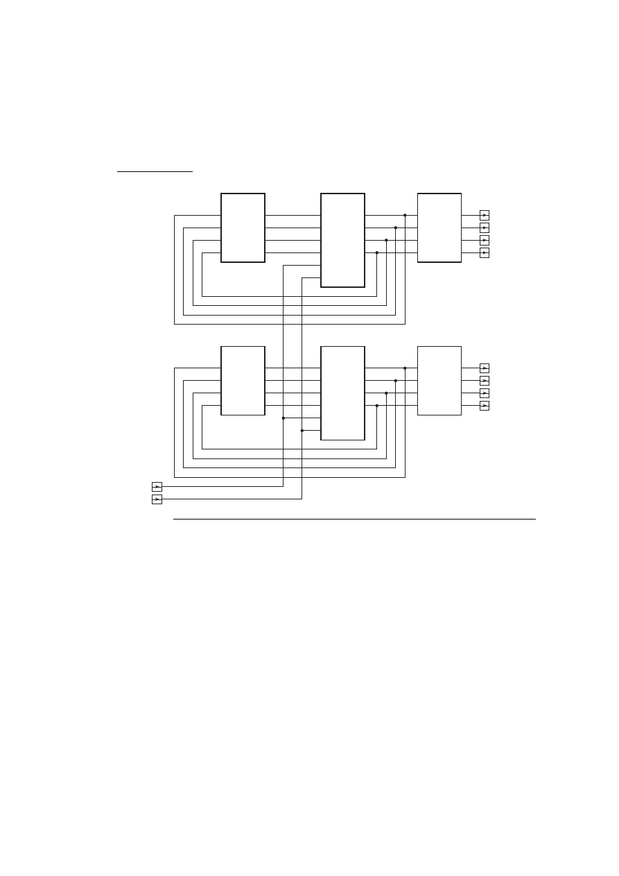
Structural Descriptions
55
––––––––––––––––––––––––––––––––––––––––––––––––––––
architecture registered of counter is
signal current_val0, current_val1, next_val0, next_val1 : digit;
begin
val0_reg : entity work.reg4(struct)
port map ( d0 => next_val0(0), d1 => next_val0(1),
d2 => next_val0(2), d3 => next_val0(3),
q0 => current_val0(0), q1 => current_val0(1),
q2 => current_val0(2), q3 => current_val0(3),
clk => clk, clr => clr );
val1_reg : entity work.reg4(struct)
port map ( d0 => next_val1(0), d1 => next_val1(1),
d2 => next_val1(2), d3 => next_val1(3),
q0 => current_val1(0), q1 => current_val1(1),
q2 => current_val1(2), q3 => current_val1(3),
clk => clk, clr => clr );
FIGURE 4-4
A schematic for a two-digit counter using the
reg4
entity.
add_1
d0
incr0
y0
y1
y2
y3
d1
d2
d3
buf4
a0
buf0
y0
y1
y2
y3
a1
a2
a3
reg4
d0
val0_reg
q0
q1
q2
q3
d1
d2
d3
clr
clk
clr
clk
add_1
d0
incr1
y0
y1
y2
y3
d1
d2
d3
buf4
a0
buf1
y0
y1
y2
y3
a1
a2
a3
reg4
d0
val1_reg
q0
q1
q2
q3
d1
d2
d3
clr
clk
q0(0)
q0(1)
q0(2)
q0(3)
q1(0)
q1(1)
q1(2)
q1(3)
56
Basic Modeling Constructs
incr0 : entity work.add_1(boolean_eqn) …;
incr1 : entity work.add_1(boolean_eqn) …;
buf0 : entity work.buf4(basic) …;
buf1 : entity work.buf4(basic) …;
end architecture registered;
An entity declaration of a two-digit decimal counter, with an outline of an architecture body using the
reg4
entity.
4.5
Libraries and Library Clauses
Earlier, we mentioned that a design is analyzed in order to check that it conforms to
the syntax and semantic rules of VHDL. An analyzed design unit, such as an entity
declaration or architecture body, is placed into a design library. A VHDL tool suite
must provide some means of using a number of separate design libraries. When a
design is analyzed, we nominate one of the libraries as the working library, and the
analyzed design is stored in this library. We use the special library name
work
in our
VHDL models to refer to the current working library. We have seen examples of this
in this chapter’s component instantiation statements, in which a previously analyzed
entity is instantiated in a structural architecture body.
If we need to access library units stored in other libraries, we refer to the libraries
as resource libraries. We do this by including a library clause immediately preceding
a design unit that accesses the resource libraries. The syntax rule for a library clause is
library_clause ⇐
library
identifier {
,
… }
;
The identifiers are used by the analyzer and the host operating system to locate
the design libraries, so that the units contained in them can be used in the description
being analyzed. The exact way that the identifiers are used varies between different
tool suites and is not defined by the VHDL language specification. Note that we do
not need to include the library name
work
in a library clause; the current working li-
brary is automatically available.
EXAMPLE
Suppose we are working on part of a large design project code-named Wasp,
and we are using standard cell parts supplied by Widget Designs, Inc. Our system
administrator has loaded the design library for the Widget cells in a directory
called /local/widget/cells in our workstation file system, and our project leader
has set up another design library in /projects/wasp/lib for some in-house cells we
need to use. We consult the manual for our VHDL analyzer and use operating
system commands to set up the appropriate mapping from the identifiers
widget_cells
and
wasp_lib
to these library directories. We can then instantiate en-
tities from these libraries, along with entities we have previously analyzed, into
our own working library, as shown in Figure 4-6.

Libraries and Library Clauses
57
FIGURE 4-6
library widget_cells, wasp_lib;
architecture cell_based of filter is
–– declaration of signals, etc
…
begin
clk_pad : entity wasp_lib.in_pad
port map ( i => clk, z => filter_clk );
accum : entity widget_cells.reg32
port map ( en => accum_en, clk => filter_clk, d => sum,
q => result );
alu : entity work.adder
port map ( a => alu_op1, b => alu_op2, y => sum, c => carry );
–– other component instantiations
…
end architecture cell_based;
An outline of a library unit referring to entities from the resource libraries
widget_cells
and
wasp_lib
.


59
5
Subprograms
5.1
Procedures
We start our discussion of subprograms with procedures. There are two aspects to
using procedures in a model: first the procedure is declared, then elsewhere the pro-
cedure is called. The syntax rule for a procedure declaration is
subprogram_body ⇐
procedure
identifier [
(
parameter_interface_list
)
]
is
{ subprogram_declarative_part }
begin
{ sequential_statement }
end
[
procedure
] [ identifier ]
;
For now we will just look at procedures without the parameter list part; we will come
back to parameters in the next section.
The identifier in a procedure declaration names the procedure. The name may
be repeated at the end of the procedure declaration. The sequential statements in the
body of a procedure implement the algorithm that the procedure is to perform and
can include any of the sequential statements that we have seen in previous chapters.
A procedure can declare items in its declarative part for use in the statements in the
procedure body. The declarations can include types, subtypes, constants, variables
and nested subprogram declarations. The items declared are not accessible outside
of the procedure; we say they are local to the procedure.
The actions of a procedure are invoked by a procedure call statement, which is
yet another VHDL sequential statement. A procedure with no parameters is called
simply by writing its name, as shown by the syntax rule
procedure_call_statement ⇐ procedure_name
;
When the last statement in the procedure is completed, the procedure returns.
We can write a procedure declaration in the declarative part of an architecture
body or a process. If a procedure is included in an architecture body’s declarative
part, it can be called from within any of the processes in the architecture body. On
the other hand, declaring a procedure within a process hides it away from use by oth-
er processes.

60
Subprograms
EXAMPLE
The outline in Figure 5-1 illustrates a procedure for arithmetic operations de-
fined within a process. The process
alu
invokes
do_arith_op
with a procedure call
statement.
FIGURE 5-1
architecture rtl of control_processor is
type func_code is (add, subtract);
signal op1, op2, dest : integer;
signal Z_flag : boolean;
signal func : func_code;
…
begin
alu : process is
procedure do_arith_op is
variable result : integer;
begin
case func is
when add =>
result := op1 + op2;
when subtract =>
result := op1 – op2;
end case;
dest <= result after Tpd;
Z_flag <= result = 0 after Tpd;
end procedure do_arith_op;
begin
…
do_arith_op;
…
end process alu;
…
end architecture rtl;
An outline of an architecture body with a process containing a procedure. The procedure encapsulates
part of the behavior of the process and is invoked by the procedure call statement within the process.
5.2
Procedure Parameters
Now that we have looked at the basics of procedures, we will discuss procedures that
include parameters. When we write a parameterized procedure, we include informa-
tion in the parameter list about the parameters to be passed to the procedure. The
syntax rule for a procedure declaration on page 59 shows where the parameter list fits
in. Following is the syntax rule for a parameter list:
Procedure Parameters
61
interface_list ⇐
( [
constant
I
variable
I
signal
]
identifier {
,
… }
:
[ mode ] subtype_indication
[
:=
static_expression ] ) {
;
… }
mode ⇐
in
I
out
I
inout
The parameter list defines the formal parameters of the procedure. We can think of
them as placeholders that stand for the actual parameters, which are to be supplied
by the caller when it calls the procedure. Since the syntax rule for a parameter list is
quite complex, let us start with some simple examples and work up from them.
EXAMPLE
First, let’s rewrite the procedure
do_arith_op
, from Figure 5-1, so that the func-
tion code is passed as a parameter. The new version is shown in Figure 5-2. In
the parameter interface list we have identified one formal parameter named
op
.
The mode of the formal parameter is
in
, indicating that it is used to pass informa-
tion into the procedure from the caller. The type of the parameter is
func_code
,
indicating that the operations performed on the formal parameter must be appro-
priate for a value of this type and that the caller may only pass a value of this type
as an actual parameter.
Now that we have parameterized the procedure, we can call it from different
places passing different function codes each time. For example, a call at one
place might be
do_arith_op ( add );
The procedure call simply includes the actual parameter value in parentheses. In
this case we pass the literal value
add
as the actual parameter. At another place
in the model we might pass the value of the signal
func
shown in the model in
do_arith_op ( func );

62
Subprograms
FIGURE 5-2
procedure do_arith_op ( op : in func_code ) is
variable result : integer;
begin
case op is
when add =>
result := op1 + op2;
when subtract =>
result := op1 – op2;
end case;
dest <= result after Tpd;
Z_flag <= result = 0 after Tpd;
end procedure do_arith_op;
A procedure to perform an arithmetic operation, parameterized by the kind of operation.
The syntax rule for a parameter list also shows us that we can specify the class of
a formal parameter, namely, whether it is a constant, a variable or a signal within the
procedure. If the mode of the parameter is
in
, the class is assumed to be constant,
since a constant is an object that cannot be updated by assignment. Usually we simply
leave out the keyword
constant
, relying on the mode to make our intentions clear.
For an
in
mode constant-class parameter, we write an expression as the actual param-
eter.
Let us now turn to formal parameters of mode
out
. Such a parameter lets us trans-
fer information out from the procedure back to the caller. Here is an example.
EXAMPLE
The procedure in Figure 5-3 performs addition of two unsigned numbers rep-
resented as bit vectors of type
word32
, which we assume is defined elsewhere.
The procedure has two
in
mode parameters
a
and
b
, allowing the caller to pass
two bit-vector values. The procedure uses these values to calculate the sum and
overflow flag. Within the procedure, the two
out
mode parameters,
result
and
overflow
, appear as variables. The procedure performs variable assignments to
update their values, thus transferring information back to the caller.
FIGURE 5-3
procedure addu ( a, b : in word32;
result : out word32; overflow : out boolean ) is
variable sum : word32;
variable carry : bit := '0';
begin
for index in sum'reverse_range loop
sum(index) := a(index) xor b(index) xor carry;
carry := ( a(index) and b(index) ) or ( carry and ( a(index) xor b(index) ) );
end loop;
result := sum;
Procedure Parameters
63
overflow := carry = '1';
end procedure addu;
A procedure to add two bit vectors representing unsigned integers.
A call to this procedure may appear as follows:
variable PC, next_PC : word32;
variable overflow_flag : boolean;
…
addu ( PC, X"0000_0004", next_PC, overflow_flag);
In the above example, the
out
mode parameters are of the class variable. Since
this class is assumed for
out
parameters, we usually leave out the class specification
variable
. The mode
out
indicates that the only way the procedure may use the formal
parameters is to update them by variable assignment; it may not read the values of
the parameters. For an
out
mode, variable-class parameter, the caller must supply a
variable as an actual parameter.
The third mode we can specify for formal parameters is
inout
, which is a combi-
nation of
in
and
out
modes. It is used for objects that are to be both read and updated
by a procedure. As with
out
parameters, they are assumed to be of class variable if
the class is not explicitly stated. For
inout
mode variable parameters, the caller sup-
plies a variable as an actual parameter. The value of this variable is used to initialize
the formal parameter, which may then be used in the statements of the procedure.
The procedure may also perform variable assignments to update the formal parame-
ter. When the procedure returns, the value of the formal parameter is copied back to
the actual parameter variable, transferring information back to the caller.
Signal Parameters
The third class of object that we can specify for formal parameters is signal, which
indicates that the algorithm performed by the procedure involves a signal passed by
the caller. A signal parameter can be of any of the modes
in
,
out
or
inout
.
The way that signal parameters work is somewhat different from constant and
variable parameters. When a caller passes a signal as a parameter of mode
in
, instead
of passing the value of the signal, it passes the signal object itself. Any reference to
the formal parameter within the procedure is exactly like a reference to the actual sig-
nal itself.
EXAMPLE
Suppose we wish to model the receiver part of a network interface. It re-
ceives fixed-length packets of data on the signal
rx_data
. The data is synchronized
with changes, from ‘0’ to ‘1’, of the clock signal
rx_clock
of part of the model.

64
Subprograms
FIGURE 5-4
architecture behavioral of receiver is
…
–– type declarations, etc
signal recovered_data : bit;
signal recovered_clock : bit;
…
procedure receive_packet ( signal rx_data : in bit;
signal rx_clock : in bit;
data_buffer : out packet_array ) is
begin
for index in packet_index_range loop
wait until rx_clock = '1';
data_buffer(index) := rx_data;
end loop;
end procedure receive_packet;
begin
packet_assembler : process is
variable packet : packet_array;
begin
…
receive_packet ( recovered_data, recovered_clock, packet );
…
end process packet_assembler;
…
end architecture behavioral;
An outline of a model of a network receiver, including a procedure with signal parameters of mode
in
.
During execution of the model, the process
packet_assembler
calls the proce-
dure
receive_packet
, passing the signals
recovered_data
and
recovered_clock
as ac-
tual parameters. The wait statement mentions
rx_clock
, and since this stands for
recovered_clock
, the process is sensitive to changes on
recovered_clock
while it is
suspended.
Now let’s look at signal parameters of mode
out
. In this case, the caller must
name a signal as the actual parameter, and the procedure is passed a reference to the
driver for the signal. When the procedure performs a signal assignment statement on
the formal parameter, the transactions are scheduled on the driver for the actual signal
parameter.
EXAMPLE
Figure 5-5 is an outline of an architecture body for a signal generator. The
procedure
generate_pulse_train
has
in
mode constant parameters that specify the
characteristics of a pulse train and an
out
mode signal parameter on which it gen-
erates the required pulse train. The process
raw_signal_generator
calls the proce-

Procedure Parameters
65
dure, supplying
raw_signal
as the actual signal parameter for
s
. A reference to the
driver for
raw_signal
is passed to the procedure, and transactions are generated
on it.
FIGURE 5-5
library ieee; use ieee.std_logic_1164.all;
architecture top_level of signal_generator is
signal raw_signal : std_ulogic;
…
procedure generate_pulse_train ( width, separation : in delay_length;
number : in natural;
signal s : out std_ulogic ) is
begin
for count in 1 to number loop
s <= '1', '0' after width;
wait for width + separation;
end loop;
end procedure generate_pulse_train;
begin
raw_signal_generator : process is
begin
…
generate_pulse_train ( width => period / 2,
separation => period – period / 2,
number => pulse_count,
s => raw_signal );
…
end process raw_signal_generator;
…
end architecture top_level;
An outline of a model for a signal generator, including a pulse generator procedure with an
out
mode
signal parameter.
As with variable-class parameters, we can also have a signal-class parameter of
mode
inout
. When the procedure is called, both the signal and a reference to its driver
are passed to the procedure. The statements within it can read the signal value, in-
clude it in sensitivity lists in wait statements, query its attributes and schedule trans-
actions using signal assignment statements.
Default Values
The one remaining part of a procedure parameter list that we have yet to discuss is
the optional default value expression, shown in the syntax rule on page 61. Note that
we can only specify a default value for a formal parameter of mode
in
, and the pa-
rameter must be of the class constant or variable. If we include a default value in a
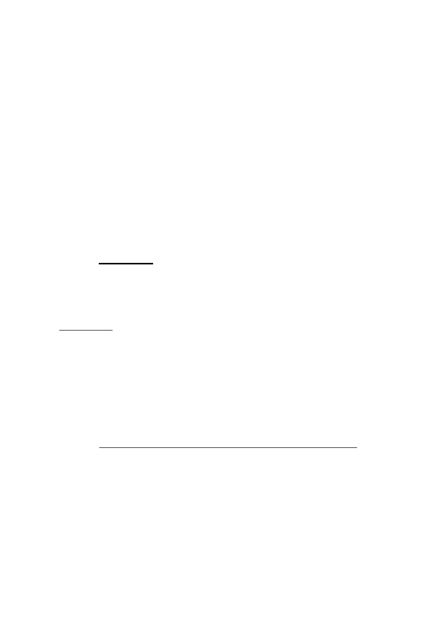
66
Subprograms
parameter specification, we have the option of omitting an actual value when the pro-
cedure is called. We can either use the keyword
open
in place of an actual parameter
value or, if the actual value would be at the end of the parameter list, simply leave it
out. If we omit an actual value, the default value is used instead.
Unconstrained Array Parameters
In an earlier chapter we described unconstrained array types, in which the index
range of the array was left unspecified using the “box” (“
<>
”) notation. For such a
type, we constrain the index bounds when we create an object, such as a variable or
a signal. Another use of an unconstrained array type is as the type of a formal param-
eter to procedure. This use allows us to write a procedure in a general way, so that
it can operate on array values of any size or with any range of index values. When
we call the procedure and provide a constrained array as the actual parameter, the
index bounds of the actual array are used as the bounds of the formal array parameter.
EXAMPLE
Figure 5-6 is a procedure that finds the index of the first bit set to ‘1’ in a bit
vector. The formal parameter
v
is of type
bit_vector
, which is an unconstrained
array type. Note that in writing this procedure, we do not explicitly refer to the
index bounds of the formal parameter
v
, since they are not known. Instead, we
use the
'range
attribute.
FIGURE 5-6
procedure find_first_set ( v : in bit_vector;
found : out boolean;
first_set_index : out natural ) is
begin
for index in v'range loop
if v(index) = '1' then
found := true;
first_set_index := index;
return;
end if;
end loop;
found := false;
end procedure find_first_set;
A procedure to find the first set bit in a bit vector.
When the procedure is executed, the formal parameters stand for the actual
parameters provided by the caller. So if we call this procedure as follows:
variable int_req : bit_vector (7 downto 0);
variable top_priority : natural;
variable int_pending : boolean;
…
find_first_set ( int_req, int_pending, top_priority );

Functions
67
v'range
returns the range
7 downto 0
, which is used to ensure that the loop pa-
rameter
index
iterates over the correct index values for
v
. If we make a different
call:
variable free_block_map : bit_vector(0 to block_count–1);
variable first_free_block : natural;
variable free_block_found : boolean;
…
find_first_set ( free_block_map, free_block_found, first_free_block );
v'range
returns the index range of the array
free_block_map
, since that is the actual
parameter corresponding to
v
.
5.3
Functions
Let us now turn our attention to the second kind of subprogram in VHDL: functions.
The syntax rule for a function declaration is very similar to that for a procedure dec-
laration:
subprogram_body ⇐
function
identifier [
(
parameter_interface_list
)
]
return
type_mark
is
{ subprogram_declarative_item }
begin
{ sequential_statement }
end
[
function
] [ identifier ]
;
The identifier in the declaration names the function. It may be repeated at the
end of the declaration. Unlike a procedure subprogram, a function calculates and re-
turns a result that can be used in an expression. The function declaration specifies
the type of the result after the keyword
return
. The parameter list of a function takes
the same form as that for a procedure, with two restrictions. First, the parameters of
a function may not be of the class variable. If the class is not explicitly mentioned, it
is assumed to be constant. Second, the mode of each parameter must be
in
. If the
mode is not explicitly specified, it is assumed to be
in
. Like a procedure, a function
can declare local items in its declarative part for use in the statements in the function
body.
A function passes the result of its computation back to its caller using a return
statement, given by the syntax rule
return_statement ⇐
return
expression
;
A function must include at least one return statement. The first to be executed causes
the function to complete and return its result to the caller. A function cannot simply
run into the end of the function body, since to do so would not provide a way of
specifying a result to pass back to the caller.
A function call looks exactly like a procedure call. The syntax rule is
function_call ⇐ function_name [
(
parameter_association_list
)
]

68
Subprograms
The difference is that a function call is part of an expression, rather than being a se-
quential statement on its own, like a procedure call.
EXAMPLE
The function in Figure 5-7 determines the number represented in binary by a
bit-vector value.
FIGURE 5-7
function bv_to_natural ( bv : in bit_vector ) return natural is
variable result : natural := 0;
begin
for index in bv'range loop
result := result * 2 + bit'pos(bv(index));
end loop;
return result;
end function bv_to_natural;
A function that converts the binary representation of an unsigned number to a numeric value.
As an example of using this function, consider a model for a read-only mem-
ory, which represents the stored data as an array of bit vectors, as follows:
type rom_array is array (natural range 0 to rom_size–1)
of bit_vector(0 to word_size–1);
variable rom_data : rom_array;
If the model has an address port that is a bit vector, we can use the function to
convert the address to a natural value to index the ROM data array, as follows:
data <= rom_data ( bv_to_natural(address) ) after Taccess;

69
6
Packages and Use Clauses
6.1
Package Declarations and Bodies
A VHDL package is simply a way of grouping a collection of related declarations that
serve a common purpose. They allow us to separate the external view of the items
they declare from the implementation of those items. The external view is specified
in a package declaration, whereas the implementation is defined in a separate pack-
age body. The syntax rule for writing a package declaration is
package_declaration ⇐
package
identifier
is
{ package_declarative_item }
end
[
package
] [ identifier ]
;
The identifier provides a name for the package, which we can use elsewhere in
a model to refer to the package. Inside the package declaration we write a collection
of declarations, including type, subtype, constant, signal and subprogram declara-
tions. These are the declarations that are provided to the users of the package.
Figure 6-1 is a simple example of a package declaration.
FIGURE 6-1
package cpu_types is
constant word_size : positive := 16;
constant address_size : positive := 24;
subtype word is bit_vector(word_size – 1 downto 0);
subtype address is bit_vector(address_size – 1 downto 0);
type status_value is ( halted, idle, fetch, mem_read, mem_write,
io_read, io_write, int_ack );
end package cpu_types;
A package that declares some useful constants and types for a CPU model.
A package is another form of design unit, along with entity declarations and ar-
chitecture bodies. It is separately analyzed and is placed into the working library as
a library unit by the analyzer. From there, other library units can refer to an item de-
clared in the package using the selected name of the item. The selected name is

70
Packages and Use Clauses
formed by writing the library name, then the package name and then the name of the
item, all separated by dots; for example:
work.cpu_types.status_value
Subprograms in Package Declarations
Another kind of declaration that may be included in a package declaration is a sub-
program declaration—either a procedure or a function declaration. An important as-
pect of declaring a subprogram in a package declaration is that we only write the
header of the subprogram, that is, the part that includes the name and the interface
list defining the parameters (and result type for functions). We leave out the body of
the subprogram. For example, suppose we have a package declaration that defines
a bit-vector subtype:
subtype word32 is bit_vector(31 downto 0);
We can include in the package a procedure to do addition on
word32
values that rep-
resent signed integers. The procedure declaration in the package declaration is
procedure add ( a, b : in word32;
result : out word32; overflow : out boolean );
Note that we do not include the keyword
is
or any of the local declarations or
statements needed to perform the addition; these are deferred to the package body.
Each package declaration that includes subprogram declarations must have a corre-
sponding package body to fill in the missing details. However, if a package declara-
tion only includes other kinds of declarations, such as types, signals or fully specified
constants, no package body is necessary. The syntax rule for a package body is sim-
ilar to that for the interface, but with the inclusion of the keyword
body
:
package_body ⇐
package
body
identifier
is
{ package_body_declarative_item }
end
[
package
body
] [ identifier ]
;
The items declared in a package body must include the full declarations of all sub-
programs defined in the corresponding package declaration. These full declarations
must include the subprogram headers exactly as they are written in the package dec-
laration. A package body may also include declarations of additional types, subtypes,
constants and subprograms. These items are used to implement the subprograms de-
fined in the package declaration. Note that the items declared in the package decla-
ration cannot be declared again in the body (apart from subprograms and deferred
constants, as described above), since they are automatically visible in the body.
EXAMPLE
Figure 6-2 shows outlines of a package declaration and a package body de-
claring arithmetic functions for bit-vector values. The functions treat bit vectors

Use Clauses
71
as representing signed integers in binary form. Only the function headers are in-
cluded in the package declaration. The package body contains the full function
bodies. It also includes a function,
mult_unsigned
, not defined in the package dec-
laration. It is used internally in the package body to implement the signed mul-
tiplication operator.
FIGURE 6-2
package bit_vector_signed_arithmetic is
function add ( bv1, bv2 : bit_vector ) return bit_vector;
function sub ( bv : bit_vector ) return bit_vector;
function mult ( bv1, bv2 : bit_vector ) return bit_vector;
…
end package bit_vector_signed_arithmetic;
––––––––––––––––––––––––––––––––––––––––––––––––––––
package body bit_vector_signed_arithmetic is
function add ( bv1, bv2 : bit_vector ) return bit_vector is …
function sub ( bv : bit_vector ) return bit_vector is …
function mult_unsigned ( bv1, bv2 : bit_vector ) return bit_vector is
…
begin
…
end function mult_unsigned;
function mult ( bv1, bv2 : bit_vector ) return bit_vector is
begin
if bv1(bv1'left) = '0' and bv2(bv2'left) = '0' then
return mult_unsigned(bv1, bv2);
elsif bv1(bv1'left) = '0' and bv2(bv2'left) = '1' then
return –mult_unsigned(bv1, –bv2);
elsif bv1(bv1'left) = '1' and bv2(bv2'left) = '0' then
return –mult_unsigned(–bv1, bv2);
else
return mult_unsigned(–bv1, –bv2);
end if;
end function mult;
…
end package body bit_vector_signed_arithmetic;
An outline of a package declaration and body that define signed arithmetic functions on integers rep-
resented as bit vectors.
6.2
Use Clauses
We have seen how we can refer to an item provided by a package by writing its se-
lected name, for example,
work.cpu_types.status_value
. This name refers to the item
status_value
in the package
cpu_types
stored in the library
work
. If we need to refer

72
Packages and Use Clauses
to this object in many places in a model, having to write the library name and package
name becomes tedious and can obscure the intent of the model. We can write a use
clause to make names from package directly visible. The syntax rules are:
use_clause ⇐
use
selected_name {
,
… }
;
selected_name ⇐ identifier
.
identifier
.
( identifier I
all
)
In one form of selected name, the first identifier is a library name and the second
is the name of a package within the library. This form allows us to refer directly to
items within a package without having to use the full selected name. For example,
we could write a use clause
use work.cpu_types.word, work.cpu_types.address;
and then refer to the used names in declarations:
variable data_word : word;
variable next_address : address;
We can place a use clause in any declarative part in a model. One way to think
of a use clause is that it “imports” the names of the listed items into the part of the
model containing the use clause.
The syntax rule for a use clause shows that we can write the keyword
all
instead
of the name of a particular item to import from a package. This form is very useful,
as it is a shorthand way of importing all of the names defined in the interface of a
package. For example, if we are using the IEEE standard-logic package as the basis
for the data types in a design, we can import everything from the standard-logic pack-
age with a use clause as follows:
use ieee.std_logic_1164.all;
Use clauses may be included at the beginning of a design unit, as well as in de-
clarative parts within a design unit. We have seen earlier how we may include library
and use clauses at the head of a design unit, such as an entity interface or architecture
body. This area of a design unit is called its context clause. The names imported here
are made directly visible throughout the design unit. For example, if we want to use
the IEEE standard-logic types in the declaration of an entity, we might write the design
unit as follows:
library ieee; use ieee.std_logic_1164.all;
entity logic_block is
port ( a, b : in std_ulogic;
y, z : out std_ulogic );
end entity logic_block;
The names imported by a use clause in this way are made directly visible in the
entire design unit after the use clause. In addition, if the design unit is a primary unit
(such as an entity declaration or a package declaration), the visibility is extended to
any corresponding secondary unit. Thus, if we include a use clause in the primary

Use Clauses
73
unit, we do not need to repeat it in the secondary unit, as the names are automatically
visible there.


75
7
Resolved Signals
7.1
IEEE Std_Logic_1164 Resolved Subtypes
VHDL provides a very general mechanism for specifying what value results from con-
necting multiple outputs together. It does this through resolved subtypes and resolved
signals, which are an extension of the basic signals we have used in previous chap-
ters. However, most designs simply use the resolved subtypes defined in the stan-
dard-logic package,
std_logic_1164
. In this tutorial, we will restrict our attention to
those subtypes.
First, recall that the package provides the basic type
std_ulogic
, defined as
type std_ulogic is ('U', 'X', '0', '1', 'Z', 'W', 'L', 'H', '–');
and an array type
std_ulogic_vector
, defined as
type std_ulogic_vector is array ( natural range <> ) of std_ulogic;
We have not mentioned it before, but the “u” in “ulogic” stands for unresolved.
Signals of these types cannot have multiple sources. The standard-logic package also
provides a resolved subtype called
std_logic
. A signals of this type can have multiple
sources. The package also declares an array type of standard-logic elements, analo-
gous to the
bit_vector
type, for use in declaring array signals:
type std_logic_vector is array ( natural range <>) of std_logic;
The standard defines the way in which contributions from multiple sources are
resolved to yield the final value for a signal. If there is only one driving value, that
value is used. If one driver of a resolved signal drives a forcing value (‘X’, ‘0’ or ‘1’)
and another drives a weak value(‘W’, ‘L’ r ‘H’), the forcing value dominates. On the
other hand, if both drivers drive different values with the same strength, the result is
the unknown value of that strength (‘X’ or ‘W’). The high-impedance value, ‘Z’, is
dominated by forcing and weak values. If a “don’t care” value (‘–’) is resolved with
any other value, the result is the unknown value ‘X’. The interpretation of the “don’t
care” value is that the model has not made a choice about its output state. Finally, if
an “uninitialized” value (‘U’) is to be resolved with any other value, the result is ‘U’,
indicating that the model has not properly initialized all outputs.
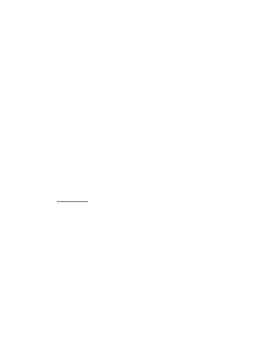
76
Resolved Signals
In addition to this multivalued logic subtype, the package
std_logic_1164
declares
a number of subtypes for more restricted multivalued logic modeling. The subtype
declarations are
subtype X01 is resolved std_ulogic range 'X' to '1';
–– ('X','0','1')
subtype X01Z is resolved std_ulogic range 'X' to 'Z';
–– ('X','0','1','Z')
subtype UX01 is resolved std_ulogic range 'U' to '1';
–– ('U','X','0','1')
subtype UX01Z is resolved std_ulogic range 'U' to 'Z';
–– ('U','X','0','1','Z')
The standard-logic package provides the logical operators
and
,
nand
,
or
,
nor
,
xor
,
xnor
and
not
for standard-logic values and vectors, returning values in the range ‘U’,
‘X’, ‘0’ or ‘1’. In addition, there are functions to convert between values of the full
standard-logic type, the subtypes shown above and the predefined bit and bit-vector
types.
7.2
Resolved Signals and Ports
In the previous discussion of resolved signals, we have limited ourselves to the simple
case where a number of sources drive a signal. Any input port connected to the re-
solved signal gets the final resolved value as the port value. We now look in more
detail at the case of a port of mode
inout
being connected to a resolved signal. The
value seen by the input side of such a port is the final value of the resolved signal
connected to the port. An
inout
port models a connection in which the driver con-
tributes to the associated signal’s value, and the input side of the component senses
the actual signal rather than using the driving value.
EXAMPLE
Some asynchronous bus protocols use a distributed synchronization mecha-
nism based on a wired-and control signal. This is a single signal driven by each
module using active-low open-collector or open-drain drivers and pulled up by
the bus terminator. If a number of modules on the bus need to wait until all are
ready to proceed with some operation, they use the control signal as follows. Ini-
tially, all modules drive the signal to the ‘0’ state. When each is ready to proceed,
it turns off its driver (‘Z’) and monitors the control signal. So long as any module
is not yet ready, the signal remains at ‘0’. When all modules are ready, the bus
terminator pulls the signal up to the ‘1’ state. All modules sense this change and
proceed with the operation.
Figure 7-1 shows an entity declaration for a bus module that has a port of the
unresolved type
std_ulogic
for connection to such a synchronization control sig-
nal. The architecture body for a system comprising several such modules is also
outlined. The control signal is pulled up by a concurrent signal assignment state-
ment, which acts as a source with a constant driving value of ‘H’. This is a value
having a weak strength, which is overridden by any other source that drives ‘0’.
It can pull the signal high only when all other sources drive ‘Z’.

Resolved Signals and Ports
77
FIGURE 7-1
library ieee; use ieee.std_logic_1164.all;
entity bus_module is
port ( synch : inout std_ulogic; … );
end entity bus_module;
––––––––––––––––––––––––––––––––––––––––––––––––––––
architecture top_level of bus_based_system is
signal synch_control : std_logic;
…
begin
synch_control_pull_up : synch_control <= 'H';
bus_module_1 : entity work.bus_module(behavioral)
port map ( synch => synch_control, … );
bus_module_2 : entity work.bus_module(behavioral)
port map ( synch => synch_control, … );
…
end architecture top_level;
An entity declaration for a bus module that uses a wired-and synchronization signal, and an archi-
tecture body that instantiates the entity, connecting the synchronization port to a resolved signal.
Figure 7-2 shows an outline of a behavioral architecture body for the bus
module. Each instance initially drives its synchronization port with ‘0’. This value
is passed up through the port and used as the contribution to the resolved signal
from the entity instance. When an instance is ready to proceed with its operation,
it changes its driving value to ‘Z’, modeling an open-collector or open-drain driver
being turned off. The process then suspends until the value seen on the synchro-
nization port changes to ‘H’. If other instances are still driving ‘0’, their contribu-
tions dominate, and the value of the signal stays ‘0’. When all other instances
eventually change their contributions to ‘Z’, the value ‘H’ contributed by the pull-
up statement dominates, and the value of the signal changes to ‘H’. This value is
passed back down through the ports of each instance, and the processes all re-
sume.
FIGURE 7-2
architecture behavioral of bus_module is
begin
behavior : process is
…
begin
synch <= '0' after Tdelay_synch;
…
–– ready to start operation
synch <= 'Z' after Tdelay_synch;
wait until synch = 'H';
–– proceed with operation

78
Resolved Signals
…
end process behavior;
end architecture behavioral;
An outline of a behavioral architecture body for a bus module, showing use of the synchronization con-
trol port.

79
8
Generic Constants
8.1
Parameterizing Behavior
VHDL provides us with a mechanism, called generics, for writing parameterized mod-
els. We can write a generic entity by including a generic list in its declaration that
defines the formal generic constants that parameterize the entity. The extended syn-
tax rule for entity declarations including generics is
entity_declaration ⇐
entity
identifier
is
[
generic
(
generic_interface_list
)
;
]
[
port
(
port_interface_list
)
;
]
end
[
entity
] [ identifier ]
;
The generic interface list is like a parameter list, but with the restriction that we
can only include constant-class objects, which must be of mode
in
. Since these are
the defaults for a generic list, we can use a simplified syntax rule:
generic_interface_list ⇐
( identifier {
,
… }
:
subtype_indication [
:=
expression ] )
{
;
… }
A simple example of an entity declaration including a generic interface list is
entity and2 is
generic ( Tpd : time );
port ( a, b : in bit; y : out bit );
end entity and2;
This entity includes one generic constant,
Tpd
, of the predefined type
time
. The value
of this generic constant may be used within the entity statements and any architecture
body corresponding to the entity. In this example the intention is that the generic
constant specify the propagation delay for the module, so the value should be used
in a signal assignment statement as the delay. An architecture body that does this is
architecture simple of and2 is
begin

80
Generic Constants
and2_function :
y <= a and b after Tpd;
end architecture simple;
A generic constant is given an actual value when the entity is used in a component
instantiation statement. We do this by including a generic map, as shown by the ex-
tended syntax rule for component instantiations:
component_instantiation_statement ⇐
instantiation_label
:
entity
entity_name
(
architecture_identifier
)
[
generic
map
(
generic_association_list
)
]
port
map
(
port_association_list
)
;
The generic association list is like other forms of association lists, but since gener-
ic constants are always of class constant, the actual arguments we supply must be ex-
pressions. Thus the simplified syntax rule for a generic association list is
generic_association_list ⇐
( [ generic_name
=>
] ( expression I
open
) ) {
,
… }
To illustrate this, let us look at a component instantiation statement that uses the
and2
entity shown above:
gate1 : entity work.and2(simple)
generic map ( Tpd => 2 ns )
port map ( a => sig1, b => sig2, y => sig_out );
The generic map specifies that this instance of the
and2
module uses the value
2 ns for the generic constant
Tpd
; that is, the instance has a propagation delay of 2 ns.
We might include another component instantiation statement using
and2
in the same
design but with a different actual value for
Tpd
in its generic map, for example:
gate2 : entity work.and2(simple)
generic map ( Tpd => 3 ns )
port map ( a => a1, b => b1, y => sig1 );
When the design is elaborated we have two processes, one corresponding to the in-
stance
gate1
of
and2
, which uses the value 2 ns for
Tpd
, and another corresponding
to the instance
gate2
of
and2
, which uses the value 3 ns.
8.2
Parameterizing Structure
The second main use of generic constants in entities is to parameterize their structure.
We can use the value of a generic constant to specify the size of an array port by using
the generic constant in constraints in the port declarations. To illustrate, here is an
entity declaration for a register:
entity reg is
generic ( width : positive );

Parameterizing Structure
81
port ( d : in bit_vector(0 to width – 1);
q : out bit_vector(0 to width – 1);
… );
end entity reg;
In this declaration we require that the user of the register specify the desired port
width for each instance. The entity then uses the width value as a constraint on both
the input and output ports. A component instantiation using this entity might appear
as follows:
signal in_data, out_data : bit_vector(0 to bus_size – 1);
…
ok_reg : entity work.reg
generic map ( width => bus_size )
port map ( d => in_data, q => out_data, … );
EXAMPLE
A complete model for the register, including the entity declaration and an ar-
chitecture body, is shown in Figure 8-1. The generic constant is used to constrain
the widths of the data input and output ports in the entity declaration. It is also
used in the architecture body to determine the size of the constant bit vector
zero
.
This bit vector is the value assigned to the register output when it is reset, so it
must be of the same size as the register port.
We can create instances of the register entity in a design, each possibly having
different-sized ports. For example:
word_reg : entity work.reg(behavioral)
generic map ( width => 32 )
port map ( … );
creates an instance with 32-bit-wide ports. In the same design, we might include
another instance, as follows:
subtype state_vector is bit_vector(1 to 5);
…
state_reg : entity work.reg(behavioral)
generic map ( width => state_vector'length )
port map ( … );
This register instance has 5-bit-wide ports, wide enough to store values of the sub-
type
state_vector
.
FIGURE 8-1
entity reg is
generic ( width : positive );
port ( d : in bit_vector(0 to width – 1);
q : out bit_vector(0 to width – 1);
clk, reset : in bit );
end entity reg;

82
Generic Constants
––––––––––––––––––––––––––––––––––––––––––––––––––––
architecture behavioral of reg is
begin
behavior : process (clk, reset) is
constant zero : bit_vector(0 to width – 1) := (others => '0');
begin
if reset = '1' then
q <= zero;
elsif clk'event and clk = '1' then
q <= d;
end if;
end process behavior;
end architecture behavioral;
An entity and architecture body for a register with parameterized port size.
Document Outline
- VHDL Tutorial
- Introduction
- Fundamental Concepts
- VHDL is Like a Programming Language
- Basic Modeling Constructs
- Subprograms
- Packages and Use Clauses
- Resolved Signals
- Generic Constants
Wyszukiwarka
Podobne podstrony:
VHDL Cookbook Peter J Ashenden
Introduction to VHDL
bugzilla tutorial[1]
lab1 VHDL
freeRadius AD tutorial
Alignmaster tutorial by PAV1007 Nieznany
free sap tutorial on goods reciept
ms excel tutorial 2013
Joomla Template Tutorial
ALGORYTM, Tutoriale, Programowanie
8051 Tutorial uart
B tutorial
Labview Tutorial
Obraz partycji (ghost2003) Tutorial
[LAB5]Tutorial do kartkówki
M2H Networking Tutorial Original
ABAQUS Tutorial belka z utwierdzeniem id 50029 (2)
więcej podobnych podstron