
CMM-2007 – Computer Methods in Mechanics
June 19–22, 2007, Łódź–Spała, Poland
Analysis of spatial shear wall structures of variable cross-section
Jacek Wdowicki and Elżbieta Wdowicka
Institute of Structural Engineering, Poznań University of Technology
Piotrowo 5, 60-965 Poznań
e-mail:
jacek.wdowicki@put.poznan.pl
Abstract
A method has been proposed for the analysis of three-dimensional shear wall and shear core assemblies with variable dimensions and
geometries. The analysis is based on a variant of the continuum method. In the continuous approach the connecting beams and
vertical joints are replaced by equivalent continuous connections. The differential equation systems for shear wall structure segments
of constant cross-section are uncoupled by orthogonal eigenvectors. The solution matches the boundary conditions of the upper and
lower part of the wall at the plane of contiguity, at which an abrupt change in cross-section occurs. This yields a system of linear
equations for the determination of the constants of integration. The correctness and efficiency of the continuous connection method is
illustrated by application of the technique to the analysis of spatial, complex wall system of variable cross-section.
Keywords: shear wall structures, variable cross-section, continuous connection method, tall buildings
1.
Introduction
The application of continuum method to the analysis of
coupled shear walls with abrupt changes in cross-section has
been considered in Ref. [7], [8], [2], [9], [6], [4], [1], [11].
The analysis of three-dimensional shear wall systems, using the
iterative technique based on a combination of the finite strip
method and the continuum method, has been presented in
Ref. [4]. In Ref. [5] discrete force method has been developed
for the solution of such problems.
The purpose of this paper is to present the effective
algorithm for the analysis of spatial shear wall structures of
variable cross-section, using the variant of continuous
connection method.
2.
Governing differential equations
Equation formulations for a three-dimensional continuous
model of the shear wall structure with the constant cross-section
have been given in Ref. [10]. A structure, which changes its
cross-section along the height, can be divided into n
h
segments,
each one being of constant cross-section. For k-th segment the
differential equations can be stated as follows:
),
(
)
(
)
(
,
(
)
(
)
(
)
(
)
(
)
(
1
z
f
z
N
z
N
h
h
z
k
k
N
k
k
N
k
k
k
=
−
′′
>
∈
−
A
B
(1)
where B
(k)
is n
w
x n
w
diagonal matrix, containing continuous
connection flexibilities, A
(k)
is n
w
× n
w
symmetric, positive
semi-definite matrix, dependent on a structure, n
w
is the number
of continuous connections, which substitute the connecting
beam bands and vertical joints, N
N(k)
(z) is a vector containing
unknown functions of the shear force intensity in continuous
connections and f
(k)
(z) is a vector formed on the basis of given
loads for the k-th segment of the shear wall structure.
The boundary conditions for the whole structure take the
following form [11]:
,
0
)
(
,
)
0
(
'
)
(
0
1
)
1
(
)
1
(
=
−
=
−
H
N
z
N
h
n
N
T
E
N
S
B
(2)
where S
E
is n
e
× n
w
boolean matrix, related to the interaction
between shear walls and continuous connections, z
0
is the vector
containing given settlements of shear walls, n
e
is the number of
shear walls, h
k
is the ordinate of k-th change of the cross-section
and H is the structure height.
In contemporary designs of tall buildings structures with
significant changes in geometry occur, such as walls with
openings missing on the lower floors or shear walls missing on
the upper floors. In order to enable an accurate analysis of these
difficult cases, the refined boundary conditions for shear force
intensity functions at the plane of contiguity, at which an abrupt
change in cross-section occurs, have been derived in the
following form:
),
(
)
(
)
1
(
)
1
(
1
)
(
)
(
k
k
N
k
k
k
k
N
h
N
h
N
+
+
−
=
B
B
(3)
),
(
)
(
))
(
)
(
(
)
(
)
(
)
(
)
(
)
1
(
)
(
1
)
(
"
)
1
(
)
1
(
)
1
(
"
)
(
)
(
)
(
1
)
(
'
)
1
(
)
1
(
1
)
(
'
)
(
k
k
E
k
S
k
S
T
k
E
k
k
k
k
T
k
N
k
k
k
T
k
N
k
k
k
N
k
k
k
k
N
h
n
h
V
h
V
h
N
h
N
K
K
S
B
L
C
L
C
B
B
B
−
+
−
+
=
+
−
+
+
+
−
+
+
−
(4)
where C
N
is the 3n
e
×n
w
matrix containing the coordinates
of the points of contraflexure in the connecting beams in the
local coordinate systems, L
is the
3n
e
×n
w
matrix of coordinates
transformation from the global 0XYZ system to the local
systems, i.e. the systems of principal axes of shear walls, V(z) is
the vector containing the functions of horizontal displacements
of the structure, K
S
is the n
e
×n
e
diagonal matrix,
K
S
= diag(1/EA
i
) and n
E
(z) is the vector containing the normal
forces in shear walls.
It should be emphasized here that the mid-points of the
connecting beams in different segments should lie on the same
vertical line. The derivation of Eqn (3) and Eqn (4) is given in
the Appendix.
After the determining of the unknown functions of shear
force intensity in continuous connections it is possible to obtain
the function of horizontal displacements of the structure as well
as its derivatives using the following equations:

CMM-2007 – Computer Methods in Mechanics
June 19–22, 2007, Łódź–Spała, Poland
),
(
)
(
)
(
,
(
)
(
)
(
)
(
)
(
''
'
)
(
1
z
N
z
T
z
V
h
h
z
k
N
k
N
k
K
k
T
k
k
k
V
V
−
=
>
∈
−
(5)
where k is the index of a segment of the constant cross
section, V(z) is the vector containing the functions of horizontal
displacements of the structure, measured in the global
coordinate system 0XYZ and T
K
(z) is the vector of the functions
of shear forces and torque resulting from lateral loads.
Matrices V
T
, V
N
appearing in the above relation are
described by the following formulae:
,
1
,
)
(
N
T
T
N
Z
T
T
C
L
V
V
L
K
L
V
=
=
−
(6)
where K
Z
is the 3n
e
× 3n
e
matrix containing transverse stiffness
of shear walls,
K
Z
= - diag (E J
y1
,…,E J
yne
, E J
x1
,…,E J
xne
, E J
ω
1
,…, E J
ω
ne
).
The boundary conditions have the following form:
.
0
)
(
,
0
)
0
(
,
0
)
0
(
''
)
(
'
)
1
(
)
1
(
=
=
=
H
V
V
V
h
n
(7)
Besides, at the stations, where the cross sections of the walls
change, the following compatibility conditions can be stated.
From the geometric compatibility consideration we have:
).
(
)
(
),
(
)
(
'
)
1
(
'
)
(
)
1
(
)
(
k
k
k
k
k
k
k
k
h
V
h
V
h
V
h
V
+
+
=
=
(8)
From equilibrium consideration the following condition is
obtained:
),
(
)
(
)
1
(
)
(
k
k
E
k
k
E
h
m
h
m
+
=
(9)
where m
E
(z) is the vector of bending moments and bi-
moments in the shear walls, described by the relation:
).
(
)
(
''
z
V
z
m
Z
E
L
K
=
(10)
Substituting Eqn (10) in Eqn (9) and then premultiplying by
V
T(k)
L
T
(k)
, the following condition is obtained:
)
(
)
(
''
)
1
(
)
,
1
(
''
)
(
k
k
k
k
V
k
k
h
V
h
V
+
+
=
S
(11)
where:
.
)
1
(
)
1
(
)
(
)
(
)
,
1
(
+
+
+
=
k
k
Z
T
k
k
T
k
k
V
L
K
L
V
S
3.
Method of solution
In the proposed method, the algorithm of solving the
differential equation system, used for structures of constant
cross-section [10], has been extended so as to enable taking the
structures of the variable section into account.
In order to uncouple differential equation systems, auxiliary
functions g
(k)
(z) satisfying these relations have been
introduced:
),
(
)
(
)
(
)
(
2
/
1
)
(
)
(
z
g
z
N
k
k
k
k
N
Y
B
−
=
(12)
where Y
(k)
is the matrix columns which are eigenvectors of
the symmetrical matrix P
(k)
= B
(k)
-1/2
A
(k)
B
(k)
1/2
.
Consequently, n
w
second-order differential equations have
been obtained in the following form:
)
(
,
)
(
)
(
,
(
)
(
2
/
1
)
(
)
(
)
(
)
(
)
(
)
(
)
(
1
z
f
Y
F
F
z
g
z
g
h
h
z
k
k
T
k
i
k
Bi
k
Bi
k
i
k
i
k
i
k
k
−
−
=
=
−
′′
>
∈
B
λ
(13)
where
)
(k
i
λ
is the i-th eigenvalue of matrix
)
(k
P
, and
)
(k
i
Y
is the eigenvector corresponding to the i-th eigenvalue.
In the analysis, a polynomial form of functions f
(k)
(z) has
been used:
).
,
...
,
(
)
(
),
(
)
(
)
(
)
1
(
0
)
(
)
(
−
=
=
s
S
S
k
k
z
z
col
z
W
z
W
z
F
z
f
(14)
The eigenvalues and eigenvectors of symmetric matrix
)
(k
P
are computed by a set of procedures realizing the Householder’s
tridiagonalization and the QL algorithm, which have been
inserted in Ref. [13] and later written in Pascal. Matrix A is
positive semi-definite, thus matrix P can also have zero
eigenvalues.
The solutions of Eqn (13) corresponding to zero eigenvalues
have the following form:
.
)))
1
(
/(
,
...
,
6
/
,
2
/
(
)
(
)
(
2
)
(
1
)
1
(
3
2
)
(
)
(
k
i
k
i
s
k
Bi
k
i
C
z
C
s
s
z
z
z
col
F
z
g
+
+
+
=
+
(15)
The form of solutions from Eqn (13) corresponding to the
non-zero eigenvalues is as follows:
),
(
)
(
)
(
)
(
2
)
(
1
)
(
)
(
)
(
z
W
r
e
C
e
C
z
g
S
k
Si
z
k
i
z
k
i
k
i
k
i
k
i
+
+
=
−
λ
λ
(16)
where C
1i(k)
,C
2i(k)
are the integration constants and r
Si(k)
are
particular solution coefficients, calculated by the indeterminate
coefficient method.
Introducing solutions described by Eqn (15), (16) into the
relation (12) and later considering boundary conditions given by
Eqn (2), Eqn (3) and Eqn (4) we will obtain the system of
2 n
h
n
w
linear equations for the determination of all the
constants of integration in the form:
,
S
W
P
C
=
R
(17)
where R
W
is an unsymmetric matrix and P
S
is a vector
dependent on the loads. The vector C successively for each
segment contains: integration constants C
1
corresponding to
zero and non-zero eigenvalues and next integration constants C
2
corresponding to the zero and non-zero eigenvalues,
respectively. The solutions are computed by the procedures
based on the LU factorization, where L is lower-triangular and
U is upper-triangular, taken from Ref. [13].
After the determination of the integration constants C, the
functions of shear force intensity in continuous connections for
each segment are computed in a given number of points. Then
they are replaced by appropriate polynomial functions using the
interpolation.
The next step of computations is the determination of
functions of horizontal displacements V(z) and their derivatives
necessary to calculate the internal forces and stresses.
The integration of functions
)
(
''
'
z
V
taking into
consideration boundary condition
0
)
(
'
'
)
(
=
H
V
h
n
and the
compatibility condition (11) yields the following expressions:
CMM-2007 – Computer Methods in Mechanics
June 19–22, 2007, Łódź–Spała, Poland
∫
∫
+
+
−
−
+
=
>
∈
=
>
∈
z
h
k
k
k
k
V
k
k
k
k
z
H
n
n
n
k
h
h
h
h
V
dt
t
V
z
V
h
h
z
dt
t
V
z
V
H
h
z
).
(
)
(
)
(
,
(
,
)
(
)
(
,
(
''
)
1
(
)
,
1
(
''
'
)
(
''
)
(
1
''
'
)
(
''
)
(
1
S
(18)
Next, integrating the above functions with regard to
boundary conditions V
(1)
(0)
= 0, V
(1)
’(0) = 0 and compatibility
conditions (8), the following is obtained:
>
∈
−
k
k
h
h
z
,
(
1
,
)
(
)
(
)
(
1
'
)
1
(
''
)
(
'
)
(
1
−
−
+
=
∫
−
k
k
z
h
k
k
h
V
dt
t
V
z
V
k
(19)
∫
−
−
−
+
=
z
h
k
k
k
k
k
h
V
dt
t
V
z
V
1
,
)
(
)
(
)
(
1
)
1
(
'
)
(
)
(
where: k = 1,…,n
h
, h
0
= 0.
In the course of determination of functions of horizontal
displacements and their derivatives the polynomial form of
functions N
N
(z) of shear force intensity in continuous
connections has been used. Hence, the results may be computed
for the arbitrary ordinates of height.
The derived Eqn (4) will have to be satisfied in an iterative
manner. To obtain the first approximation we shall assume that
the last two terms of Eqn. (4) are equal to zero. From this
analysis the values of V”
(k)
(h
k
), V”
(k+1)
(h
k
) and n
E(k)
(h
k
) can be
found and then, according to Eqn (4), the improved value of the
vector P
S
in the Eqn (17) is obtained. The analysis then carries
on repeatedly, when the solution is found to be sufficiently
convergent. In spite of the number of iterations required, the
calculation is very fast.
Based on the presented algorithm, the software included in
the system for the analysis of shear wall tall buildings [10], [11]
in the Turbo Delphi from Borland Developer Studio 2006
environment has been implemented.
4.
Numerical examples
While testing the program for the analysis of shear wall
systems of variable cross-section there has been a good
agreement of our results, those presented in Ref. [7], [8], [2],
[6], [4], [1], [3], [4], [5] and those obtained from the tests on
Araldite models [2]. In order to verify the algorithm for the
boundary cases a number of simple examples have been
prepared, for which it was possible to estimate the values of
solutions. To illustrate the correctness of the algorithm
realization, three examples have been chosen.
4.1. Plane wall with variable cross-section and without
continuous connections
As the first example a 20-storey plane wall (Fig. 1) with an
abrupt change in cross-section at the 10
th
storey and with stiff
vertical joint in the mid-point has been analyzed.
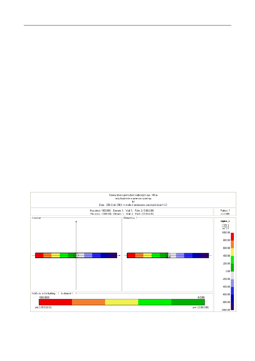
Figure 1: Normal stresses at the base of plane shear wall without continuous connections
CMM-2007 – Computer Methods in Mechanics
June 19–22, 2007, Łódź–Spała, Poland
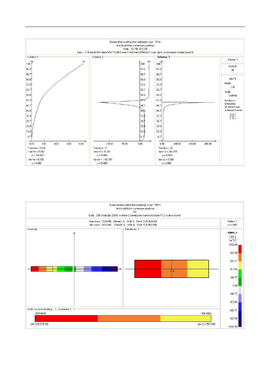
Figure 2: Horizontal displacements and shear force intensity functions in connecting beams
in plane shear wall with three continuous connections
Figure 3: Normal stresses at the base of plane shear wall with three continuous connections
CMM-2007 – Computer Methods in Mechanics
June 19–22, 2007, Łódź–Spała, Poland
The lower and upper segments are each 50 m high,
with corresponding cross-section dimensions 10 x 0.6 m and
5 x 0.6 m, respectively. The wall is subjected to a horizontal
point load P = 100 kN, acting at the top of structure. The
Young’s modulus is 30 GPa and the Kirchhoff’s modulus is 15
GPa. The horizontal displacement at the top of this structure
equals to 41.67 mm. The theoretical value of the shear force in
the stiff joint is 15 kN/m in segment 1 (lower) and 30 kN/m in
segment 2 (upper). Maximum value of the normal stresses at the
base is 1000 kPa. The computed values of displacements, shear
forces and normal stresses is equal to the theoretical ones. The
results for the next considered shear wall system will be
compared with the results for this example. The normal stresses
at the base of the structure are shown in Fig.1.
4.2. Plane shear wall of variable cross-section with three
continuous connections of small flexibility
The above described structure has been subsequently
divided into the four walls each with a depth of 2.5 m,
connected by three continuous connections of very small
flexibility (the stiffness 2717 MN/m
2
has been taken). In the
upper segment the left and right walls that are missing, have
been taken with a depth of 0.06
mm . Introducing continuous
connections of very small flexibility into the structure should
results in a slight increase in the displacements. The solution
converged to four significant figures in 5 iterations. The value
of the horizontal displacement at the top of the structure
obtained in the first iteration was 74.06 mm and the final value
was 42.31 mm. Figure 2 shows the diagrams of displacements
and the functions of shear force intensity in continuous
connections. The vertical normal stresses at the base are shown
in Fig. 3. The results were as expected and close to those
obtained from previous example.
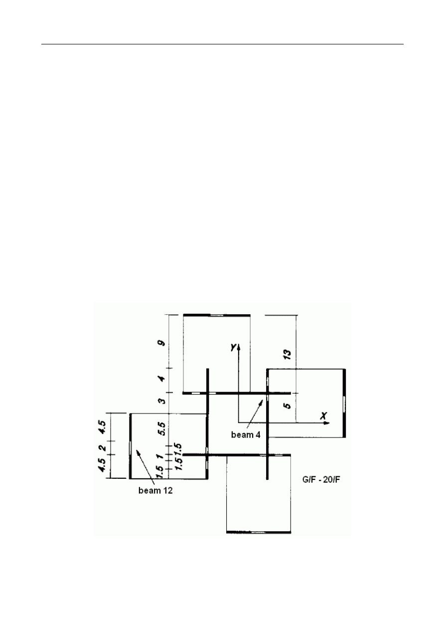
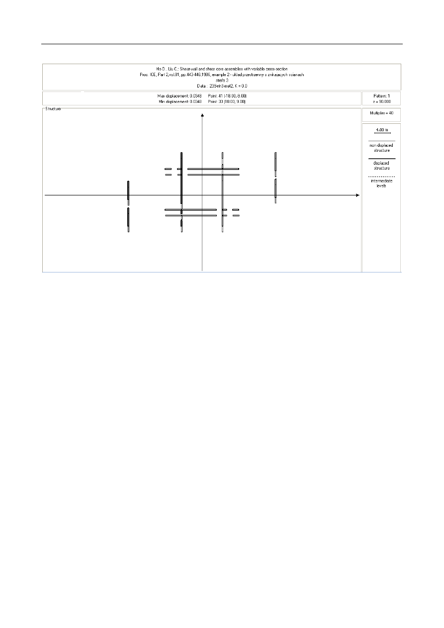
4.3. Spatial shear wall system of variable cross-section
Figure 4 shows a shear wall and shear core assembly of 30
storeys, analyzed in Ref. [4], [5]. The central core, which
houses the lift shaft and the staircase, changes its geometry at
the 20
th
floor, above which both the top-left and the bottom-
right wings of the core are missing. The thickness of the core
wall also varies from 0.15 m at 20
th
-30
th
floors to 0.2 m at
10
th
-20
th
floors, and finally to 0.3 m at 1
st
–10
th
floors.
The thickness of the exterior plane shear walls, meanwhile,
remains constant - 0.2 m. There are two types of lintel beam:
those over windows having a depth of 1 m and those over
doorways with a depth of 0.6 m. The storey height is 3.0 m.
The Young’s modulus E = 31 GPa and Poisson’s ratio ν = 0.2
are assumed for the concrete properties. A uniformly distributed
load of 50 kN/m, acting in the Y direction, is applied along the
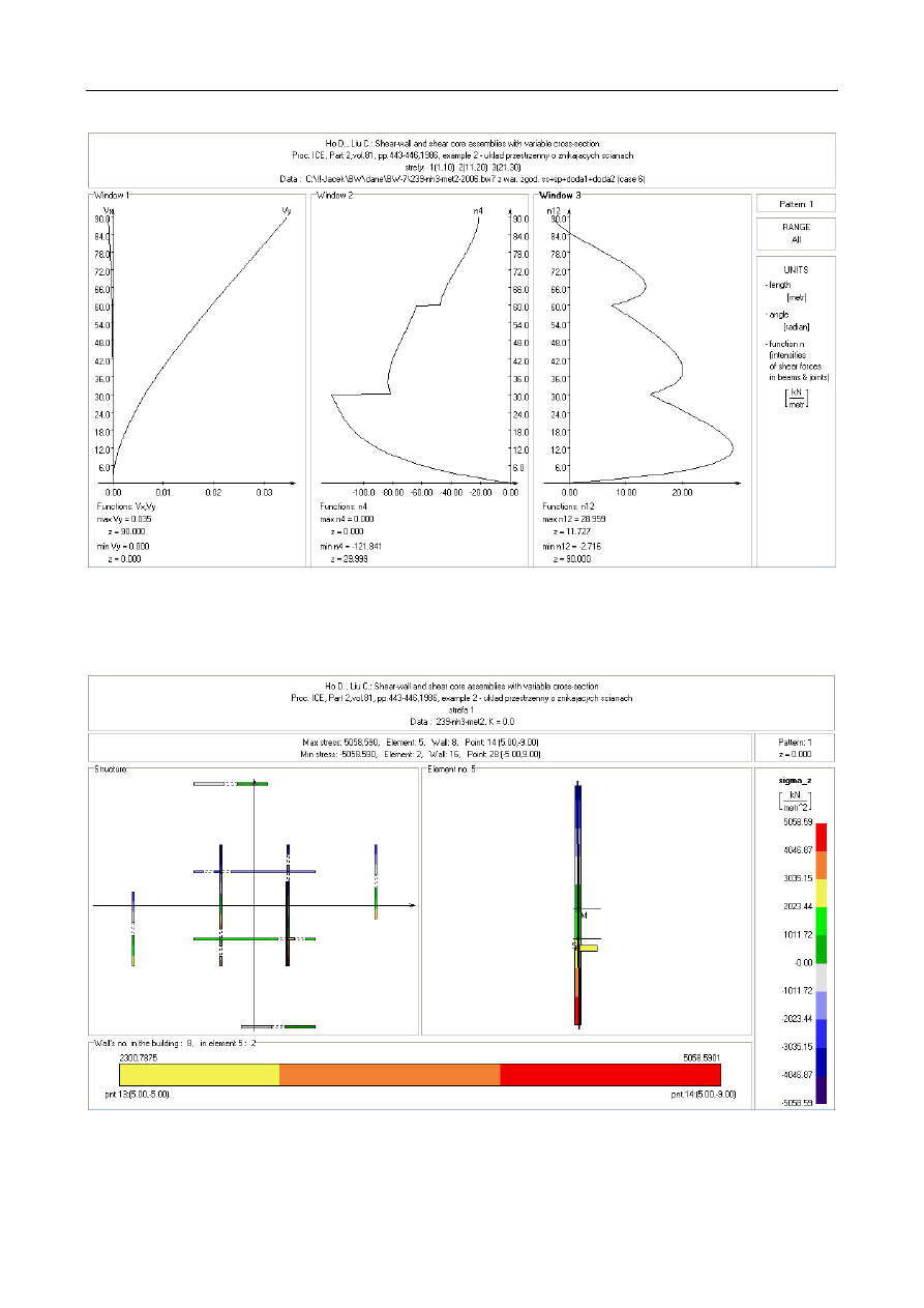
height of the structure. The obtained horizontal displacements
and distribution of shear force intensity in two bands of lintel
beams are shown in Fig. 5. Figure 6 shows normal stresses at
the base of the analyzed structure. In Fig. 7 there are the
horizontal displacements at the top of the structure. The solution
converged to four significant figures in 6 iterations. The
computations correlated well with the results of the discrete
force method presented in Ref. [5].
Figure 4: Plan of the spatial shear wall system
CMM-2007 – Computer Methods in Mechanics
June 19–22, 2007, Łódź–Spała, Poland
Figure 5: Horizontal displacements and shear force intensity functions in connecting beams
in spatial shear wall system
Figure 6: Normal stresses at the base of the spatial shear wall system
CMM-2007 – Computer Methods in Mechanics
June 19–22, 2007, Łódź–Spała, Poland
Figure 7: Displacements at the top of the spatial shear wall system
5.
Conclusions
The paper presents the algorithm for the analysis of three-
dimensional shear wall structures of variable cross-section,
using a variant of continuous connection method. The refined
boundary conditions for derivatives of shear force intensity
functions have been included. The correctness and efficiency
of the continuum method is illustrated by the application of
the technique in the analysis of a spatial, complex structure.
Acknowledgement The financial support by Poznan
University of Technology, grant DS-11-650/07 is kindly
acknowledged.
6.
References
[1] Cheung, Y.K., Au, F.T.K. and Zheng, D.Y., Analysis of
deep beams and shear walls by finite strip method with C0
continuous displacement functions, Thin-Walled Structures,
32, pp. 289-303, 1998.
[2] Coull, A., Puri, R.D. and Tottenham, H., Numerical elastic
analysis of coupled shear walls, Proceedings of the
Institution of Civil Engineers, Part 2, 55, pp. 109-128,
1973.
[3] Ha, K.H. and Tan, T.M.H., An efficient analysis of
continuum shear wall models, Canadian Journ. of Civ.
Engineering, 26, pp. 425-433, 1999.
[4] Ho, D. and Liu, C.H., Shear-wall and shear-core assemblies
with variable cross-section, Proceedings of the Institution of
Civil Engineers, 81, pp.433-446, 1986.
[5] Johnson, D. and Nadjai, A., Static analysis of spatial shear
wall systems by a discrete force method, Structural
Engineering Review, 8, 2/3, pp. 133-144, 1996.
[6] Lis, Z., Calculations of tall buildings braces with stepped
characteristics,
Archiwum
Inżynierii
Lądowej,
23,
pp. 527-534, 1977 (in Polish).
[7] Pisanty, A. and Traum, E.E., Simplified analysis of coupled
shear walls of variable cross-section, Building Science, 5,
pp.11-20, 1970.
[8] Rosman, R., Analysis of coupled shear walls, Arkady,
Warszawa 1971 (in Polish).
[9] Tso, W.K. and Chan, P.C.K., Static analysis of stepped
coupled walls by transfer matrix method, Building Science,
8, pp. 167-177, 1973.
[10] Wdowicki, J. and Wdowicka, E., System of programs for
analysis of three-dimensional shear wall structures, The
Structural Design of Tall Buildings, 2, pp. 295- 305, 1993.
[11] Wdowicki, J., and Wdowicka, E., Analysis of shear wall
structures of variable thickness using continuous connection
method, in: 16th International Conference on Computer
Methods in Mechanics, Częstochowa, Poland, 291-292 + on
CD 1-6, June 21-24, 2005.
[12] Wdowicki J.: Static analysis of three-dimensional shear
wall structures, Part I: Equations of problem, Part II:
Solution of problem equations, Computer Methods in Civil
Engineering, 3, 1, pp. 9-30, 1993 (in Polish).
[13] Wilkinson J.H. and Reinsch C.: Linear Algebra, Handbook
for Automatic Computation, vol. II, Springer-Verlag, Berlin,
Heidelberg, New York, 1971.

CMM-2007 – Computer Methods in Mechanics
June 19–22, 2007, Łódź–Spała, Poland
Appendix
Derivation of boundary conditions for the functions of shear
force intensity in continuous connections at each station
In the derivation of Eqn (3) and Eqn (4) presented below,
the following equation, obtained on the basis of compatibility
consideration at the mid-points of the cut connecting beams [12]
has been used:
)
(
)
(
)
(
'
z
V
z
V
z
N
Z
T
E
L
T
N
N
S
C
B
−
=
(A1)
where V
L
(z) = L V(z) and V
Z
(z) is the vector containing the
functions of vertical displacements of shear walls.
At the top of the k-th segment Eqn (A1) may be written as
).
(
)
(
)
(
)
(
)
(
'
)
(
)
(
)
(
)
(
)
(
k
k
Z
T
k
E
k
k
k
T
k
N
k
k
N
k
h
V
h
V
h
N
S
L
C
B
−
=
(A2)
In the next, (k+1)-th segment, the compatibility equation
(A1) may be written in the form:
).
(
)
(
)
(
)
(
)
(
'
)
(
)
1
(
)
1
(
)
(
)
(
)
1
(
)
1
(
'
)
1
(
)
1
(
)
1
(
)
1
(
)
1
(
k
k
k
T
k
N
k
T
k
N
k
Z
T
k
E
k
k
T
k
N
k
N
k
h
V
z
V
z
V
z
N
+
+
+
+
+
+
+
+
+
−
+
−
=
L
C
L
C
S
L
C
B
(A3)
The last term takes into account the vertical displacement of
the origin of local coordinate system of shear wall in the upper,
(k+1)-th segment, due to a slope of the shear wall at the top of
the lower, k-th segment.
Using the boundary conditions (8) Eqn (A3) at the bottom
of the (k+1)-th segment may be re-written as:
).
(
)
(
)
(
)
1
(
)
1
(
'
)
(
)
(
)
(
)
1
(
)
1
(
k
k
Z
T
k
E
k
k
k
T
k
N
k
k
N
k
h
V
h
V
h
N
+
+
+
+
−
=
S
L
C
B
(A4)
Using the compatibility condition for vertical displacements
of shear walls V
Z
(z) :
)
(
)
(
)
1
(
)
(
k
k
Z
k
k
Z
h
V
h
V
+
=
(A5)
and assuming that matrix S
E
is constant for each segment,
it may be noticed that right sides of Eqn (A2) and Eqn (A4) are
equal. This yields the equation:
.
)
(
)
1
(
)
1
(
)
(
)
(
+
+
=
k
N
k
k
k
N
k
N
h
N
B
B
(A6)
By pre-multiplying Eqn (A6) by B
(k)
-1
, the boundary
condition, described by Eqn (3) is obtained.
To obtain the boundary condition, described by Eqn (4), the
following condition for normal forces in shear walls, taken from
the equilibrium consideration, is used:
).
(
)
(
)
1
(
)
(
k
k
E
k
k
E
h
n
h
n
+
=
(A7)
After differentiating Eqn (A1) and Eqn (A3) we get
respectively:
)
(
)
(
'
)
(
)
(
"
)
(
)
(
)
(
'
)
(
)
(
z
V
z
V
N
k
Z
T
k
E
k
k
T
k
N
k
N
k
S
L
C
B
−
=
(A8)
and
.
)
(
'
)
1
(
)
1
(
"
)
1
(
)
1
(
)
1
(
'
)
1
(
)
1
(
+
+
+
+
+
+
+
−
=
k
Z
T
k
E
k
k
T
k
N
k
N
k
V
z
V
N
S
L
C
B
(A9)
The axial deformations and axial forces in shear walls are
related by
)
(
)
(
)
(
)
(
'
)
(
z
n
z
V
k
E
k
S
k
Z
K
=
(A10)
Substituting Eqn (A10) in Eqn (A8) and Eqn (A9), for z = h
k
the following is obtained:
)
(
)
(
)
(
)
(
)
(
)
(
"
)
(
)
(
)
(
'
)
(
)
(
k
k
E
k
S
T
k
E
k
k
k
T
k
N
k
k
N
k
h
n
h
V
h
N
K
S
L
C
B
−
=
(A11)
and
).
(
)
(
)
(
)
1
(
)
1
(
)
1
(
"
)
1
(
)
1
(
)
1
(
'
)
1
(
)
1
(
k
k
E
k
S
T
k
E
k
k
k
T
k
N
k
k
N
k
h
n
h
V
h
N
+
+
+
+
+
+
+
+
−
=
K
S
L
C
B
(A12)
Subtracting Eqn (A12) from Eqn (A11), assuming that
S
E(k+1)
= S
E(k)
and using Eqn (A7), the following is obtained:
).
(
)
(
)
(
)
(
)
(
)
(
)
(
)
(
)
1
(
)
(
"
)
1
(
)
1
(
)
1
(
"
)
(
)
(
)
(
'
)
1
(
)
1
(
'
)
(
)
(
k
k
E
k
S
k
S
T
k
E
k
k
k
T
k
N
k
k
k
T
k
N
k
k
N
k
k
k
N
k
h
n
h
V
h
V
h
N
h
N
K
K
S
L
C
L
C
B
B
−
+
−
=
−
+
+
+
+
+
+
(A13)
By pre-multiplying each term with B
(k)
-1
, the boundary
condition described by Eqn (4) is obtained.
Wyszukiwarka
Podobne podstrony:
Analysis of shear wall structures of variable thickness using continuous connection method
„SAMB” Computer system of static analysis of shear wall structures in tall buildings
Rates of NSSI A Cross Sectional Analysis of Exposure
SEISMIC ANALYSIS OF THE SHEAR WALL DOMINANT BUILDING USING CONTINUOUS-DISCRETE APPROACH
Butterworth Finite element analysis of Structural Steelwork Beam to Column Bolted Connections (2)
GL Syntax The analysis of sentence structure
Analysis of Reinforced Concrete Structures Using ANSYS Nonlinear Concrete Model
GL Morphology The analysis of word structure
Butterworth Finite element analysis of Structural Steelwork Beam to Column Bolted Connections (2)
An%20Analysis%20of%20the%20Data%20Obtained%20from%20Ventilat
[2001] State of the Art of Variable Speed Wind turbines
A Contrastive Analysis of Engli Nieznany (3)
Analysis of soil fertility and its anomalies using an objective model
Pancharatnam A Study on the Computer Aided Acoustic Analysis of an Auditorium (CATT)
więcej podobnych podstron