Tutorial 1

Helius:MCT™ Version 2.0 for Abaqus
July, 2009

Abstract

This document provides a step-by-step tutorial that demonstrates the use of Helius:MCT. The primary
emphasis is the creation of Abaqus input files that are compatible with Helius:MCT and the viewing of
special solution variables that are computed by Helius:MCT. Tutorial 1 demonstrates the use of
Abaqus/CAE in building an Abaqus input file.

For questions, comments or further information, contact Firehole Technologies at
[e-mail]












Legal Notices

Copyright 2009, Firehole Technologies, Inc.

Helius:MCT is a trademark of Firehole Technologies, Inc. Any use of the Helius:MCT trademark requires the prior
written consent of Firehole Technologies, Inc.

Abaqus/Standard is a trademark of Dassault Systemes S.A. and Dassault Systemes SIMULIA Corp

.

Page 2 of 24

Table of Contents

1

Introduction............................................................................................................................................ 3

2

Tutorial Steps ........................................................................................................................................ 4

2.1

Creating the part............................................................................................................................ 4

2.2

Creating a user material with Helius:MCT .................................................................................... 5

2.3

Defining a composite layup ........................................................................................................... 7

2.4

Defining an assembly .................................................................................................................. 11

2.5

Creating an analysis step ............................................................................................................ 12

2.6

Defining field output requests ...................................................................................................... 13

2.7

Applying boundary conditions ..................................................................................................... 15

2.8

Defining the load ......................................................................................................................... 16

2.9

Meshing the part.......................................................................................................................... 17

2.10

Creating and submitting a job ..................................................................................................... 20

2.11

Viewing and interpreting the results ............................................................................................ 21

3

Summary ............................................................................................................................................. 24

Table of Figures

Figure 1. Dimensions and loading of composite plate .................................................................................. 3
Figure 2. Plate dimensions ............................................................................................................................ 5
Figure 3. Helius:MCT GUI ............................................................................................................................. 7
Figure 4. Edit Composite Layup dialog box .................................................................................................. 9
Figure 5. Ply-1 orientation ........................................................................................................................... 10
Figure 6. Shell Parameters ......................................................................................................................... 11
Figure 7. Edit Step dialog box ..................................................................................................................... 13
Figure 8. Edit Field Output Request dialog box .......................................................................................... 14
Figure 9. Location (red) of bottom surface boundary condition .................................................................. 15
Figure 10. Location of top surface (red) load boundary condition .............................................................. 16
Figure 11. Element hourglass stiffness settings ......................................................................................... 18
Figure 12. Plate mesh ................................................................................................................................. 19
Figure 13. Edit keywords dialog box ........................................................................................................... 20
Figure 14. Failure plot of ply 1 at the end of the step ................................................................................. 22
Figure 15. Envelope plot of SDV1 at the end of the step ............................................................................ 23

Page 3 of 24

Helius:MCT Tutorial 1

Note: The following tutorial is intended to be used with Abaqus/CAE Version 6.8. As a result, some of
the results will be different if Abaqus/CAE Version 6.7 is used.

1

Introduction

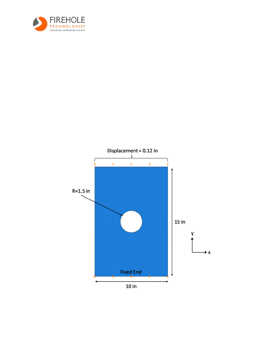
The following tutorial provides step-by-step instructions to create and analyze a simple composite plate
using the Helius:MCT GUI in ABAQUS CAE™. The problem consists of a flat composite plate with a
hole in the center subject to fixed boundary conditions on one end, and a displacement controlled load of
0.12” (0.8% of the plate length) on the other end. The plate is made of IM7/8552; the layup is [0/±45/90]

s

,

and the ply thickness is 0.005” which results in a plate thickness of 0.04”. The seed size for the mesh is
0.2, and reduced integration continuum shell elements (SC8R) are used. The dimensions, boundary
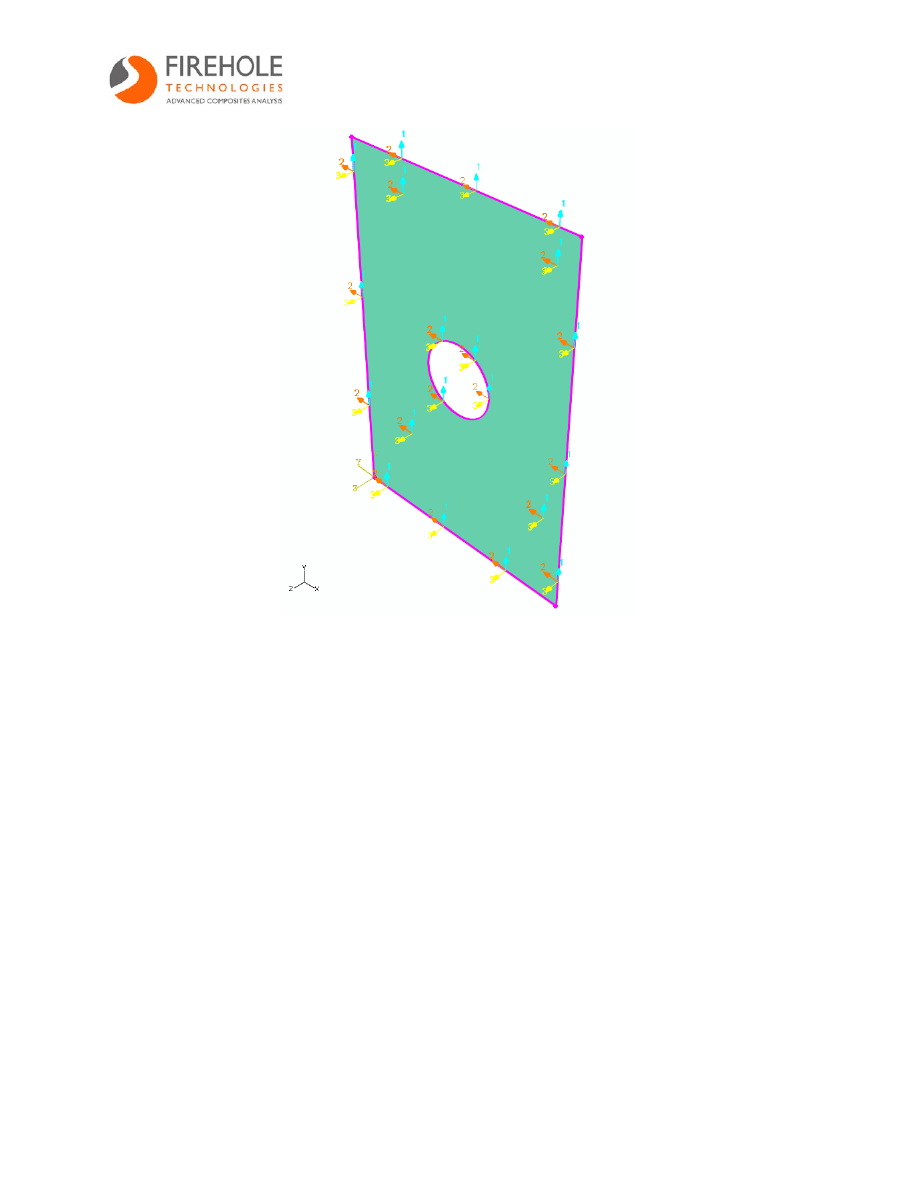
conditions, and load are shown in Figure 1. After the model is created and the finite element analysis is
completed, steps are provided to view and interpret the results.

Figure 1: Dimensions and loading of composite plate

If one is interested only in learning how to interpret Helius:MCT’s results, an ABAQUS input file
(Helius_Tutorial_1_Abaqus_Completed_v2.inp) is available for download from Firehole’s internet based
User Portal that can be used to generate an ABAQUS output (*.odb) file. In this case, run the input file
and skip to Section 2.11.

Page 4 of 24

2

Tutorial Steps

In the following tutorial, elementary modeling details are omitted as it is assumed that the user has
previous experience in the ABAQUS CAE environment. For example, it is assumed that the user knows
how to switch from module to module so that when an instruction tells the user to switch to the Mesh
module, the instructions to perform that task are omitted. Please refer to the ABAQUS documentation
before completing this tutorial if you are unfamiliar with ABAQUS CAE.

2.1 Creating the part

Defining the part geometry is generally the first step in the development of a finite element model. Here,
the plate geometry is sketched and extruded to generate a solid part.

1. Open Abaqus/CAE Version 6.8.

2. Select the Create Model Database button from the Start Session dialog box.

3. In the Model Tree, double-click the Parts container

or click Part  Create from the main

toolbar.

4. In the Create Part dialog box that appears, name the part Composite_Plate and accept the

default selections of 3D, Deformable, Solid, Extrusion and Approximate size of 200.

5. Using the Create Lines: Rectangle tool

, create a rectangle with the starting corner at

coordinates 0, 0 and the opposite corner at coordinates 10, 15.

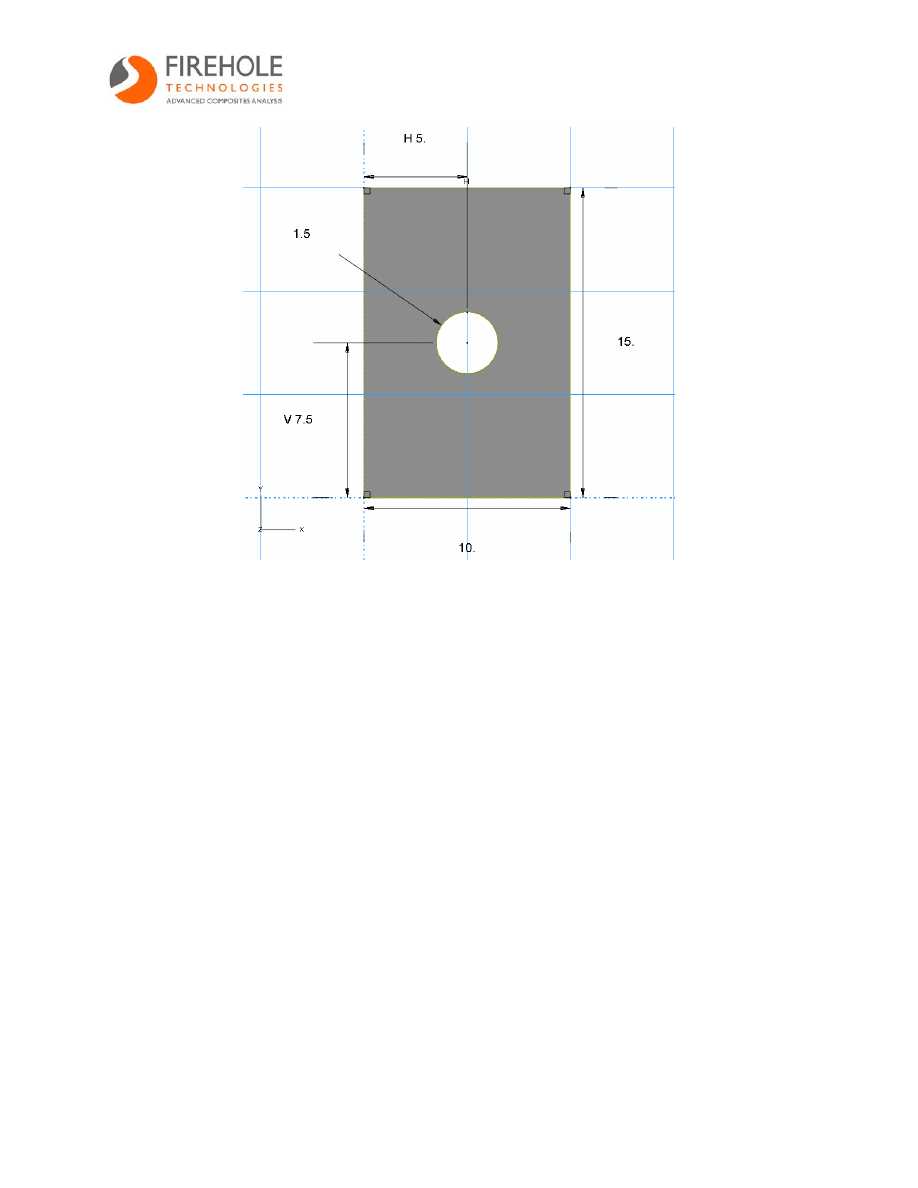
6. Using the Create Circle: Center and Perimeter tool

, create a circle with the center point at

coordinates 5, 7.5 and the perimeter point at coordinates 5, 9. The section sketch is now complete

and is shown in Figure 2 with dimensions.

7. Click the button followed by the

button to finish the sketch.

8. In the Edit Base Extrusion dialog box that appears, enter a value of 0.04 in the depth field since

there are 8 0.005” plies. Click OK.

Page 5 of 24

Figure 2: Plate dimensions

2.2 Creating a user material with Helius:MCT

The Helius:MCT plug-in is the central interface between the user and Helius:MCT. It allows the user to
choose from a variety of material and analysis options including the following:

• Choice of material

• 4 unit systems

• Fiber direction

• Progressive failure analysis

• Pressure induced strength enhancement

• Pre-failure and post-failure nonlinearity

• Degraded matrix and fiber stiffness ratios

• Viewing fiber and matrix stresses and strains

• State variable naming

Using these options, the user can tailor his or her analysis to the requirements of the problem. For a
detailed discussion of the options available, refer to Section 3.1 of the User’s Manual.

In the following steps, a user-material is created for the plate, and progressive failure analysis is
requested using the Helius:MCT plug-in.

Page 6 of 24

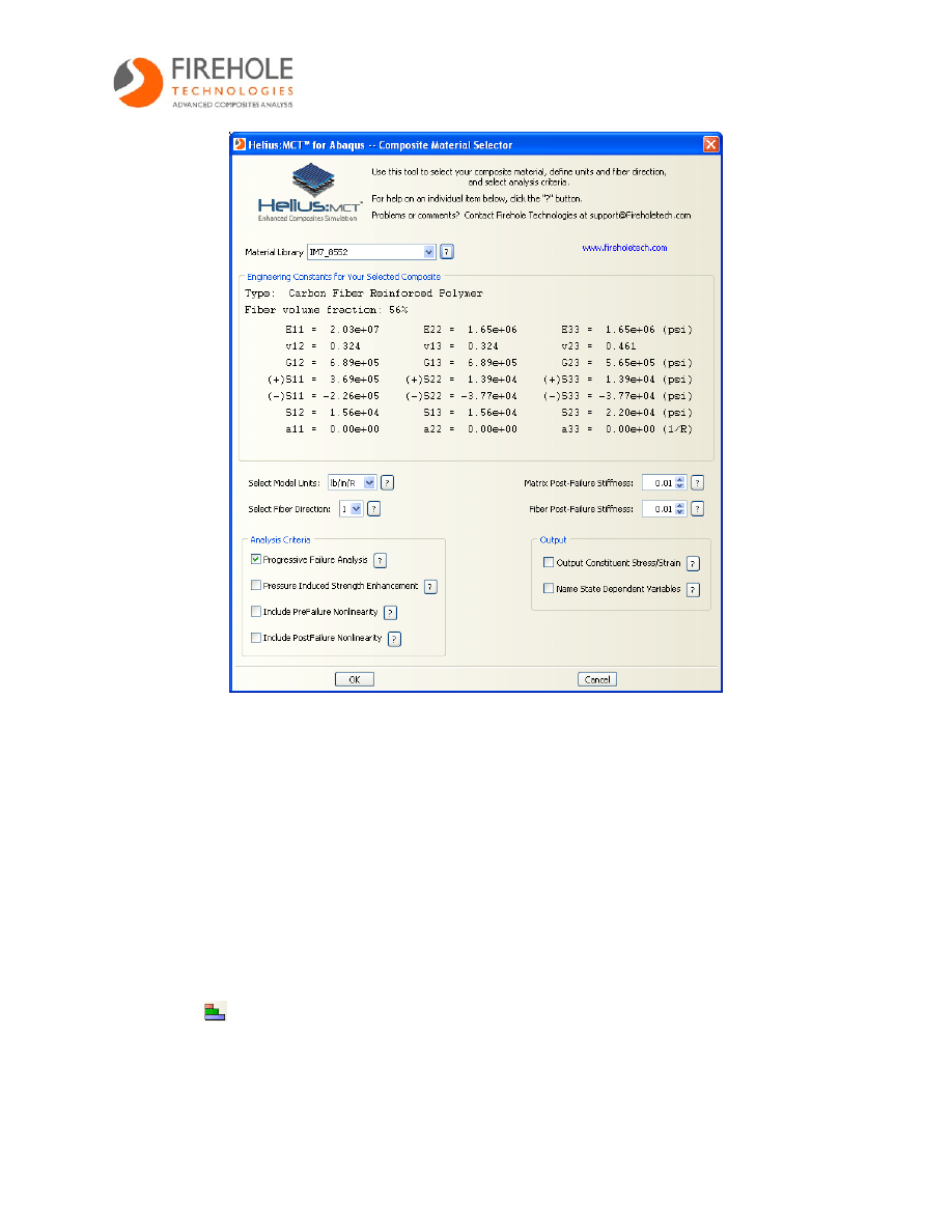
1. Select Plug-ins  Helius:MCT from the main toolbar. The Helius:MCT for Abaqus dialog

box appears.

2. From the Material Library list, select the material IM7_8552.

Note that the unit dependent Engineering Constants specific to this material are listed in

the dialog box for the user to review.

3. Since this model uses inches and pounds as base units, select lb/in/R from the Select Model

Units list.

There are 4 unit systems to choose from. The default unit system is N/m/K.

4. Select 1 as the fiber direction.

2 can also be used as the fiber direction, but it would require a different composite layup

orientation than the 1 direction. As a general rule, it is recommended that 1 be used as the

fiber direction to maintain consistency from model to model. On occasion, however, it

will not be possible to create an orientation in Abaqus that allows for the 1 direction to be

the fiber direction due to the combination of complex model geometry and orientation

limitations. In such cases, it may be necessary to use the 2 direction as the fiber direction.

5. Accept the default settings for the Analysis Criteria and Output options.

In this tutorial, only progressive failure is included in the analysis because it is the

foundation for Helius:MCT’s nonlinear multiscale constitutive model. The remaining

analysis options are included in subsequent Example Problems.

6. Set the Matrix Post-Failure Stiffness and Fiber Post-Failure Stiffness values to 0.01.

These values specify the ratio of damaged matrix and fiber moduli to undamaged fiber

and matrix stimuli. For example, a value of 0.01 means that the damaged fiber moduli

values will be 1% of the undamaged moduli values.

7. The dialog box should appear as shown in Figure 3.

8. Click OK.

9. For Ansys 11 users only: Enter MP,EX,9004,1e7 into the command prompt.

This value is used to fill a place holder required by Ansys 11 when using layered elements

and user-defined materials. The value of EX does not affect the results.

After completing steps 1-8, a user material is created in the Materials container

in the Material Tree.

This material is used to define the composite layup for the plate.

Page 7 of 24

Figure 3: Helius:MCT GUI

2.3 Defining a composite layup

After the part and the material have been created, a composite layup section can be created. The
composite layup editor is used to create plies and to assign materials and orientations to these plies.

In this step, a composite layup that represents the plate layup is created and defined. The composite layup
editor is then used to view ply orientations and verify the choice of fiber direction.

1. Switch to the Property module.

2. From the main toolbar, select Composite  Create or click on the Create Composite Layup

icon

in the toolbar.

3. In the dialog box that appears, name the layup PlateLayup, specify an initial ply count of 8,

and choose Continuum Shell for the element type. Click Continue.

Page 8 of 24

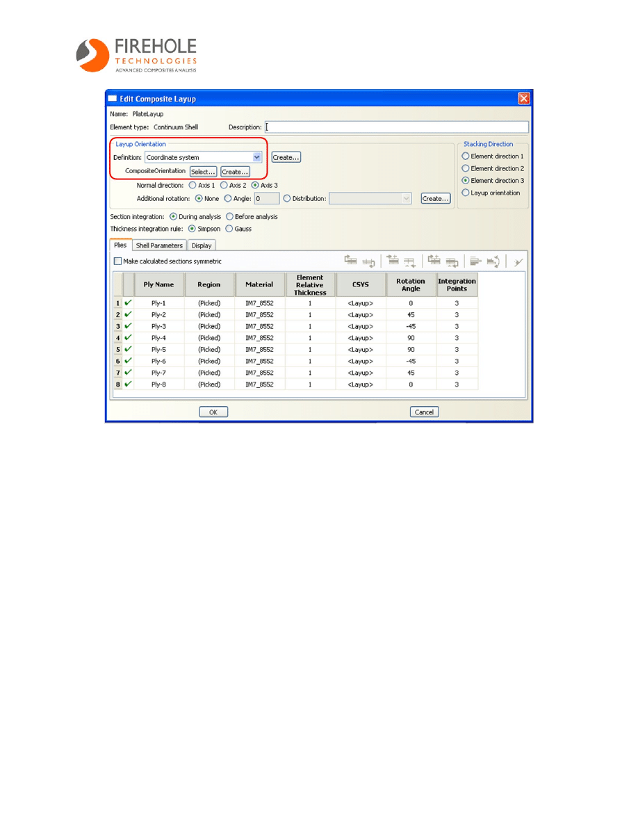
4. In the Edit Composite Layup dialog box that appears, choose Coordinate system from the

Definition drop-down list.

In Abaqus 6.7, select the CSYS radio button.

5. A datum coordinate system needs to be created to orient the plies. In the Layup Orientation box,

click the Create button that lies inside the red box highlighted in Figure 4.

6. In the dialog box that appears, name the coordinate system CompositeOrientation. Accept

the default rectangular type, and click Continue.

7. Enter 0,0,0 as the coordinates for the origin, 0,1,0 as the X-axis coordinates, and -1,0,0 as the X-

Y plane point coordinates. To submit a coordinate, press the Enter button on your keyboard

instead of clicking the Create Datum button. Click Cancel when prompted to create another

datum system.

8. The Edit Composite Layup dialog box will reappear. Click on the Select button. From the

viewport, click the Datum CSYS List... button and select CompositeOrientation from the

dialog box that appears. Click OK.

9. In the dialog box that reappears, select the plate from the viewport as the Region, IM7_8552 as

the Material, and 1 as the Element Relative Thickness. Tip: to edit all plies at once, right-click

on the Region, Material, and Element Relative Thickness buttons and select the Edit option (the

option at the top of the menu).

10. Enter the Rotation Angle for Ply-1 thru Ply-8 as 0, 45, -45, 90, 90, -45, 45, 0, respectively. The

dialog box should appear as shown in Figure 4.

Page 9 of 24

Figure 4: Edit Composite Layup dialog box

11. Click on the Rotation Angle entry for Ply-1. The orientation of Ply-1 is now shown relative to

the plate in the viewport. Check to make sure that Ply-1 has the orientation shown in Figure 5.

The 1-axis in the figure below represents the fiber direction since 1 was specified as the

fiber direction in the Helius:MCT dialog box (section 1.2). If 2 was specified as the fiber

direction, then the 2-axis would represent the fiber direction.

Page 10 of 24

Figure 5: Ply-1 orientation

Helius:MCT uses a *User Material definition instead of a *Elastic definition to define a
material in Abaqus. When a *User Material definition is used, Abaqus is unable to compute
certain section parameters because the elastic constants necessary to compute these section
parameters are not available. The user must define these parameters in order for an analysis to run
successfully. The method used to determine the values of these parameters is explained in Appendix
B.3 of the Helius:MCT User’s Guide. The section parameters for this tutorial have already been
computed and are listed in the following steps:

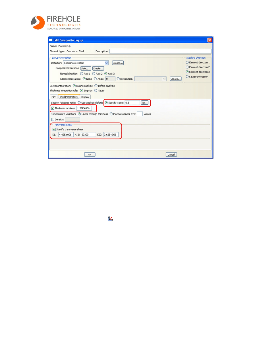
12. Select the Shell Parameters tab from the Edit Composite Layup dialog box.

13. Enter 0.5 as the value for the Section Poisson’s ratio, 1.38e6 for the Thickness Modulus, 4.42e6

for K11, 63300 for K12, and 3.62e6 for K22. The Shell Parameters tab should appear as shown

in Figure 6.

14. Click OK.

Page 11 of 24

Figure 6: Shell Parameters

2.4 Defining an assembly

In order to apply boundary conditions, loads, etc., an instance of the part must be added to the assembly.

1. Switch to the Assembly module.

2. Double click the Instances icon

in the model tree or select Instance  Create from the

main toolbar.

3. In the Create Instance dialog box that appears, click OK to accept the default option of a

Dependent instance.

Page 12 of 24

2.5 Creating an analysis step

Here, a step is defined that allows boundary conditions and output requests to be added to the model.
Nonlinear solution controls tailored for Helius:MCT are also specified that allow for a robust, converged
solution.

1. Switch to the Step module

2. Double click the Steps icon

in the model tree or select Step  Create from the main toolbar.

3. In the Create Step dialog box that appears, name the step ApplyLoad and accept the default

selection of a Static, General Procedure type. Click Continue.

4. The Edit Step dialog box appears. Select the Incrementation tab and specify an Initial

increment size of 0.05, a Minimum of 1e-10, and a Maximum of 0.05.

For a progressive failure analysis, it is necessary to adjust the default incrementation so

that the initiation and progression of both fiber and matrix failure can be viewed in a

post-processor.

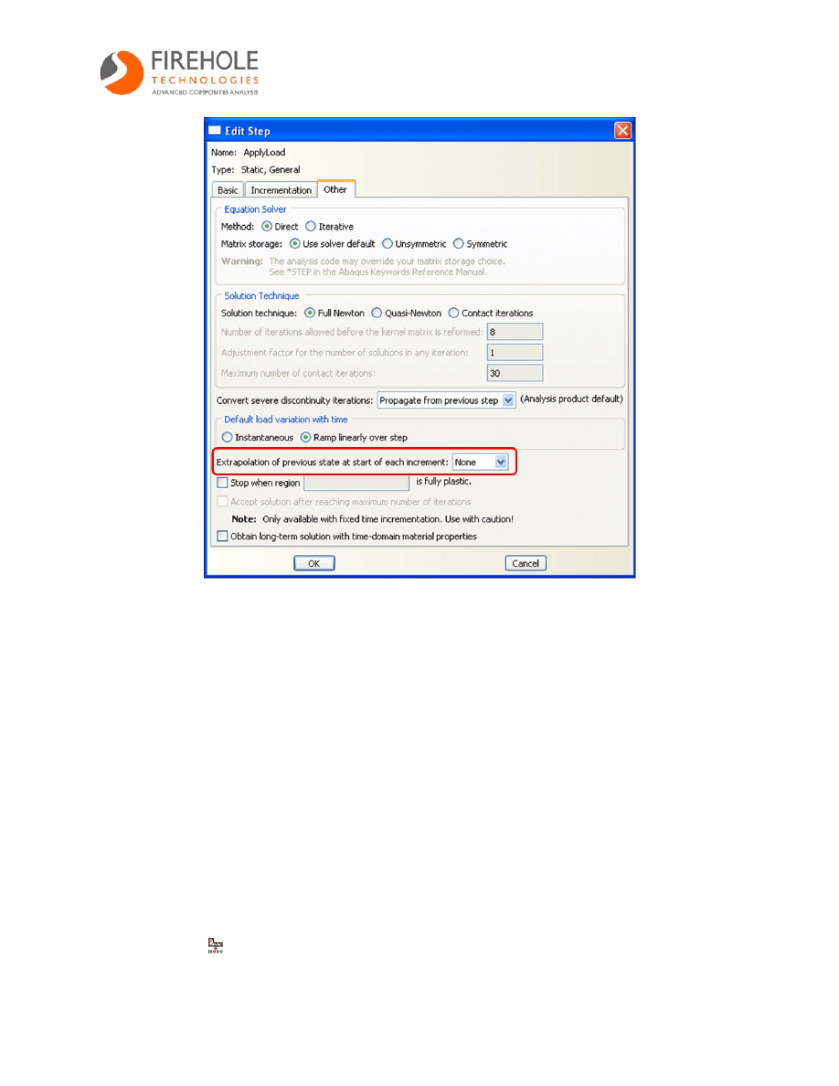
5. Select the Other tab and set the Extrapolation option to None as shown in Figure 7.

Extrapolation is set to None to avoid premature fiber failure. For further information, refer to

Helius:MCT Technical Manual.

6. Click OK.

Page 13 of 24

Figure 7: Edit Step dialog box

7. Open the General Solution Controls dialog box by clicking Other  General Solution

Controls  Edit  Apply Load from the main toolbar and click the Specify radio button.

8. From the Time Incrementation tab enter 1000 for the values of both I

0

and I

R

.

9. Click the first tab labeled ‘more’ and enter 1000 for the values of I

P

, I

C

, I

L

, and I

S

. Set I

T

to 10.

Increasing these specific values will ensure that Abaqus can take full advantage of the

improved convergence characteristics provided by Helius:MCT.

2.6 Defining field output requests

In order to use Abaqus Viewer to examine the fiber and matrix failure states generated by Helius:MCT™,
the user must request that the state variables (SDV) be printed in the ABAQUS output (odb) file.

1. Open the Edit Field Output Request dialog box by expanding the Field Output Requests

container

in the model tree and double clicking on F-Output-1, or by selecting Output 

Page 14 of 24

Field Output Requests  Manager from the main toolbar and selecting Edit in the dialog box

that appears.

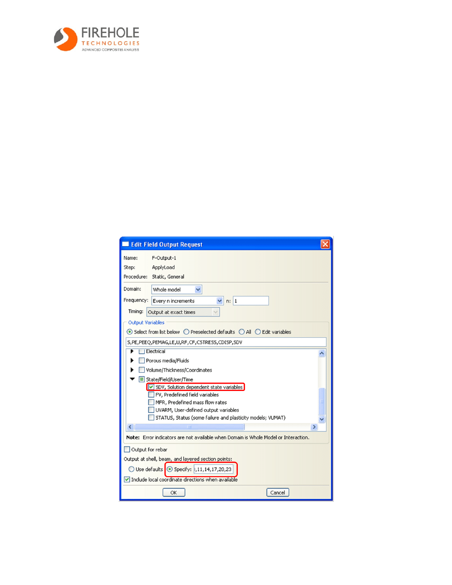
2. Add SDV to the list of Output Variables by checking the SDV box as shown in Figure 8. The

state variables will now be printed in the ABAQUS output (.odb) file.

In order to view results for each ply in the composite layup, section point output must be specified for
each ply since the default setting will only output at the top and bottom section points of the layered
element. In this tutorial, there are 8 plies with 3 section points per ply for a total of 24 section points. One
option is to specify output only from the middle section point for each ply. A second option is to specify
output for each section point in the layup. Here, output is specified for the middle section points of each
material ply.

3. Specify output at section points 2, 5, 8, 11, 14, 17, 20, 23. The Edit Field Output Request dialog

box should now appear as shown in Figure 8.

4. Click OK.

Figure 8: Edit Field Output Request dialog box

Page 15 of 24

2.7 Applying boundary conditions

The following steps create a boundary condition that fixes the bottom surface of the plate:

1. Switch to the Load module.

2. Double click on the BCs icon

in the model tree or select BC  Create from the main toolbar.

The Create Boundary Condition dialog box appears.

3. Name the boundary condition FixedBottom and click Continue to accept the default

selections of Mechanical and Symmetry/Antisymmetry/Encastre.

4. Select the bottom surface of the plate from the viewport as the region for the boundary condition

as shown in Figure 9. Be sure to select the bottom surface instead of one of the edges on the

bottom surface. Click on the Done button in the viewport.

5. In the dialog box that appears select the PINNED (U1 = U2 = U3 = 0) option and click OK.

Figure 9: Location (red) of bottom surface boundary condition

Page 16 of 24

2.8 Defining the load

A second boundary condition is created to impose a vertical displacement along the top surface of the
plate. The plate is loaded by imposing displacements because it results in a much more gradual failure
process than a comparable loading by applied forces. When a simple structure, such as this composite
plate, begins to fail under the action of applied forces, the structure fails very rapidly because the load
continues to increase as the load carrying capacity of the structure decreases. With displacement
controlled loading, the load carried by the structure decreases as the structure fails which allows for a
slower rate of failure.

1. Double click on the BCs icon

in the model tree or select BC  Create from the main toolbar.

The Create Boundary Condition dialog box appears.

2. Name the boundary condition TopLoad and select Displacement/Rotation in the Types for

Selected Step list. Click Continue.

3. Select the top surface of the plate from the viewport as the region for the boundary condition as

shown in Figure 10. Be sure to select the top surface instead of one of the edges on the top

surface. Click on the Done button in the viewport. The Edit Boundary Condition dialog box

appears.

4. Enter a value of 0.12 in the U2 field and click OK.

Figure 10: Location of top surface (red) load boundary condition

Page 17 of 24

2.9 Meshing the part

In meshing the composite plate, an approximate seed size of 0.2 is used to ensure that the mesh is fine
enough to capture the location and propagation of failure, but also coarse enough for a short solution time.

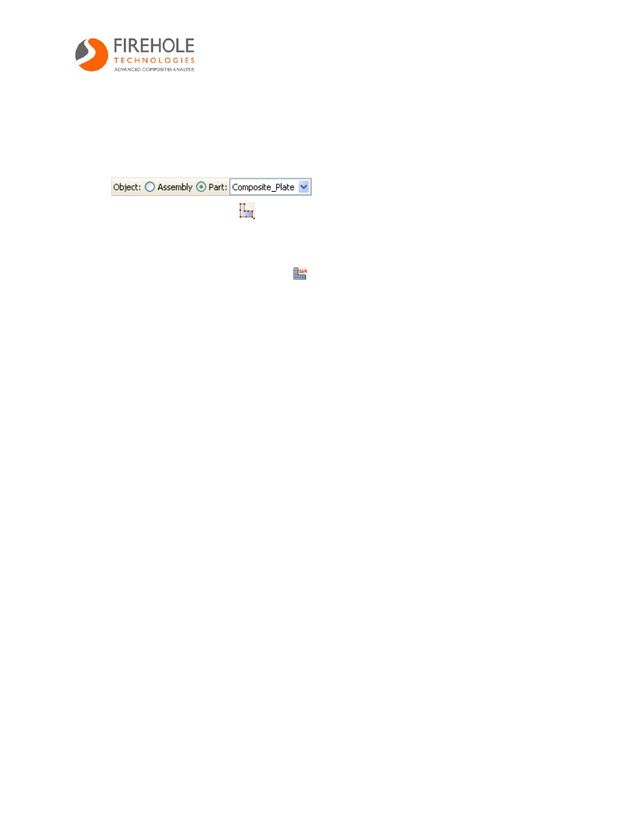
1. Switch to the Mesh module, and make sure that the Object toolbar option is set to Part.

2. Click on the Seed Part icon

or select Seed  Part from the main toolbar. The Global Seeds

dialog box appears.

3. Enter 0.2 in the approximate global size field. Click OK.

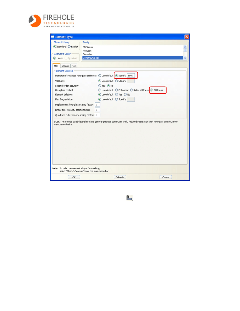
4. Click on the Assign Element Type icon

or select Mesh  Element Type from the main

toolbar. The Element Type dialog box appears.

5. Select the Continuum Shell Element SC8R.

6. From the Hourglass control options, select Stiffness. Specify a value of 3445 for

Membrane/Thickness hourglass stiffness. The dialog box should appear as shown in Figure 11.

Click OK. For Abaqus Version 6.7, skip to step 7.

a. As discussed in section 1.3, the membrane stiffness must be specified since these

elements have a *User Material material definition. For further information, see

Appendix B.3 of the Helius:MCT User’s Guide.

b. A second hourglass stiffness parameter, bending stiffness, needs to be specified as well.

At the moment, the bending stiffness can only be specified using the keywords editor and

by modifying the input file. Steps 8 and 9 below describe adding this parameter using the

keywords editor.

Page 18 of 24

Figure 11: Element hourglass stiffness settings

7. Mesh the part by clicking on the Mesh Part icon

or by selecting Mesh  Part from the main

toolbar. Click the Yes button. The mesh should be similar to the mesh shown in Figure 12.

The part must be meshed before proceeding to the next step. Meshing the part will write

the *Hourglass Stiffness keyword to the keywords editor.

Page 19 of 24

Figure 12: Plate mesh

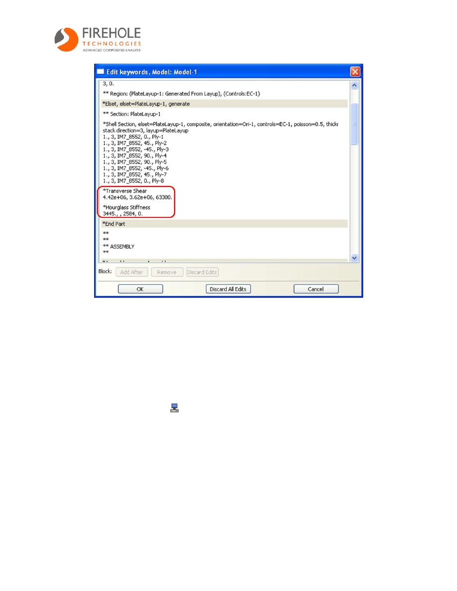
8. Click on Model  Edit Keywords  Model-1 from the main toolbar. The Edit keywords dialog

box appears.

9. Locate the *Hourglass Stiffness keyword and replace the third term with 2584 as shown in

Figure 13. Click OK.

a. The first term is the membrane stiffness parameter, and the third term is the bending

stiffness parameter. For further information, refer to the Abaqus Keywords Reference

Manual in the Abaqus documentation.

b. Note that there is currently a bug in Abaqus version 6.7 that does not allow the hourglass

stiffness to be entered in the Element Type dialog box. As a remedy, the *Hourglass

Stiffness keyword and parameters can be manually added to the keywords editor so that it

appears as shown in Figure 13.

c. A bug in Abaqus 6.7 also prevents Transverse Shear values (Section 1.3, step 13) from

automatically being written to the keywords editor. These values should be manually

entered in the keywords editor as shown in Figure 13.

Page 20 of 24

Figure 13: Edit keywords dialog box

2.10 Creating and submitting a job

The model is now completely defined and ready to be submitted for analysis. In this step, a job is created
and submitted for analysis.

1. To create a job, switch to the Job module.

2. Double click the Jobs icon

in the model tree or select Job  Create from the main toolbar.

The Create Job dialog box appears.

3. Name the job Helius_Tutorial_1 and click Continue. The Edit Job dialog box appears.

4. Accept the default job selections and click OK.

5. Select Job  Submit  Helius_Tutorial_1 from the main toolbar.

The analysis time will vary from computer to computer, but should be less than ten

minutes.

Page 21 of 24

2.11 Viewing and interpreting the results

Helius:MCT generates several state variable outputs. In this step, a key variable (SDV1) is viewed and
discussed. SDV1 is the state variable that keeps track of fiber and matrix failure within an element.

1. After the job has completed, click Job  Results  Helius_Turotial_1. This will open the

output database file and switch to the Visualization module. The undeformed plate appears in the

viewport.

2. State variable SDV1 is used to identify the discrete damage state of the composite material. To

plot this variable, select Result  Field Output from the main toolbar. The Field Output dialog

box appears.

3. Select SDV1 from the list of Output Variables. Click OK.

4. Choose Contour from the Select Plot State dialog box that appears, then click OK.

5. The elements will appear to be heavily distorted because the deformation scale factor is set too

high. Adjust the Deformation Scale Factor by selecting Options  Common from the main

toolbar and entering a value of 1 in the Deformation Scale Factor field in the Common Plot

Options dialog box. Click OK.

6. The default Contour Type is Banded, but the Quilt type is more useful for viewing SDV1 output.

To switch from Banded to Quilt, select Options  Contour from the main toolbar, and select

Quilt as the Contour Type. Click OK. The plot should be similar to the plot shown in Figure 14.

Minor differences are usually the result of mesh variations. Results generated using Abaqus 6.7

will be different because the SC8R element formulation changed from version 6.7 to version 6.8.

The following table lists the three possible values for SDV1 and the corresponding failure state. It can be
helpful to decrease the number of Contour Intervals to 3 and specify user-defined limits so that the
element colors remain consistent. For example, if there are 12 intervals and only matrix failure, Abaqus
will automatically adjust the limits to range from 1 to 2 and red elements will correspond to matrix failure
but when fiber failure occurs, the range will be adjusted to 1-3 so that red elements correspond to fiber
failure instead of matrix failure. By setting the number of Contour Intervals to 3 and specifying
appropriate user-defined limits, the range of values of SDV1 will be always be 1 to 3.

Value of SDV1

Failure State

1

No failure

2

Matrix failure

3

Fiber and matrix failure

Page 22 of 24

Figure 14: Failure plot of ply 1 at the end of the step

Note that the default ply for the contour plot shown in Figure 14 is Ply-1. To view failure in all of the
plies, envelope plots can be used. Envelope plots display the maximum or minimum integration point
value across all of the section points in each element. For example, let Ply-3 of an element be the only
failed ply in that element. The envelope plot for that element will show the element as failed, even though
no other plies in that element have failed.

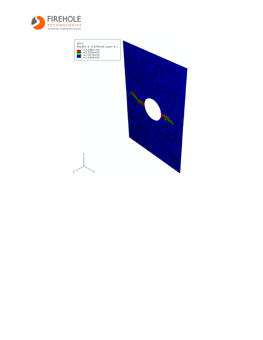
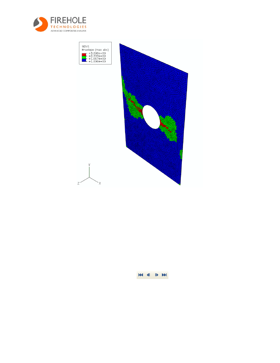
7. To create an envelope plot, select Result  Section Points from the main toolbar. Select the

Envelope option from the Categories box and click Apply. The plot should be similar to the plot

shown in Figure 15.

Page 23 of 24

Figure 15: Envelope plot of SDV1 at the end of the step

8. To view the failure state of a single ply, click Plies from the Section Points dialog box. View the

failure in each ply. Note that plies with the same orientation have identical failure states since the

laminate is symmetric. For example, Ply-2 and Ply-7 have the same failure states.

Viewing the progression of failure is often useful for visualizing the way a structure fails.

9. Switch back to the envelope plot.

10. Select Result  Step/Frame from the main toolbar. A list of each increment in the step appears.

As an alternative, the step controls

on the toolbar can be used.

11. Starting at Step Time = 0.000, progress through the step while watching the viewport to

determine when failure initiates and how failure propagates.

a. First matrix failure should occur at Step Time = 0.4500.

b. First fiber failure should occur at Step Time = 0.8500.

Page 24 of 24

3

Summary

A composite plate with a hole was modeled, and Helius:MCT was used to predict progressive fiber and
matrix failure caused by a displacement controlled load. Five different procedures specific to
Helius:MCT were used:

1. In section 2.2, the Helius:MCT plug-in was used to generate a user material.
2. In section 2.3, shell section parameters were defined for the composite layup.
3. In section 2.5, extrapolation was set to none and solution controls were defined.
4. In section 2.6, state variable (SDV) output to the database file (.odb) was requested.
5. In section 2.9, hourglass controls were specified.

After the analysis job was completed, Abaqus Viewer was used to plot fiber and matrix failure in
individual plies, and an envelope contour plot was used to view the maximum damage state that occurred
in the 8-ply laminate.