1 

 

Abaqus/CAE 

(ver. 6.8)

 Vibrations Tutorial 

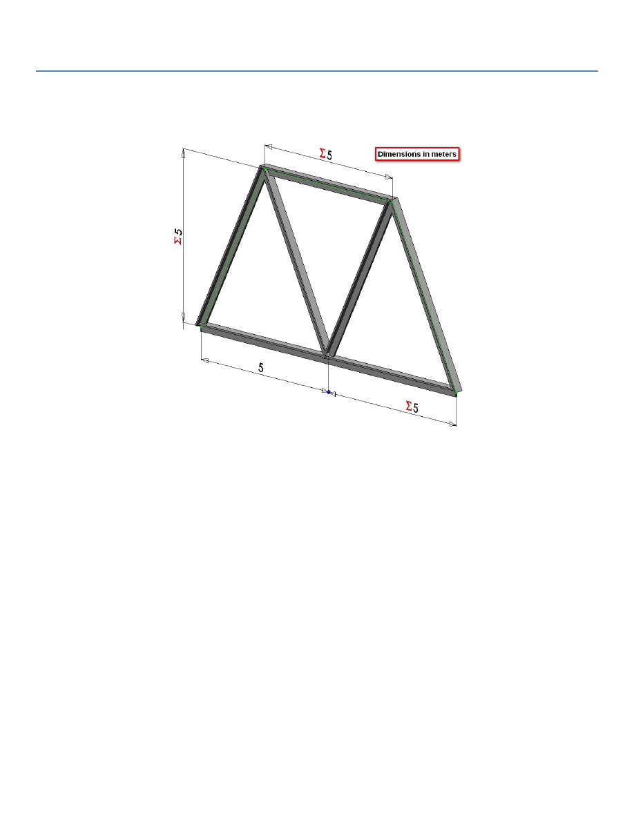
Problem Description 

 

 

The two dimensional bridge structure, which consists of steel T‐sections, is simply supported at its lower corners. 
Determine the first 10 eigenvalues and natural frequencies. 

2 

 

Analysis Steps 

1. Start Abaqus and choose to create a new model database 
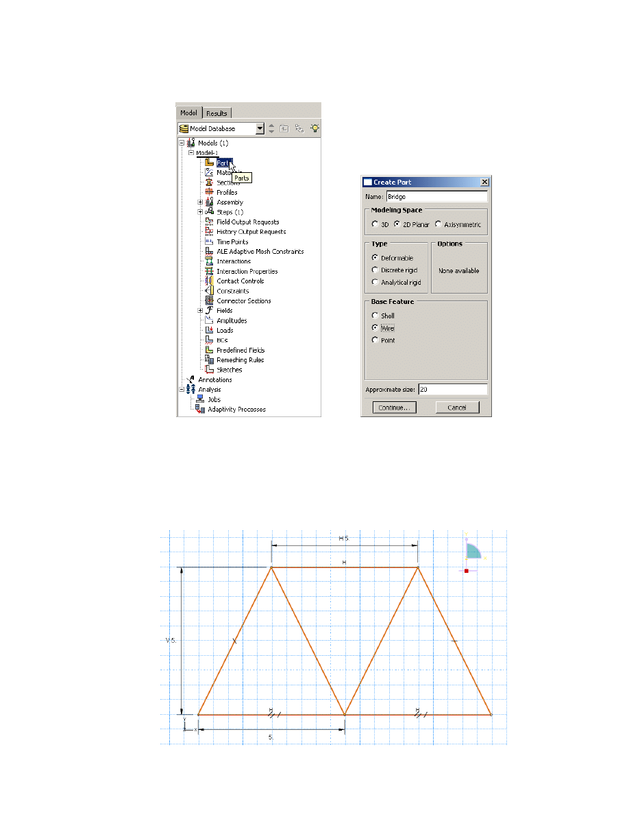
2. In the model tree double click on the “Parts” node (or right click on “parts” and select Create) 

  

 

3. In the Create Part dialog box (shown above) name the part and 

a. Select “2D Planar” 
b. Select “Deformable” 
c. Select “Wire” 
d. Set approximate size = 20 
e. Click “Continue…” 

4. Create the geometry shown below (not discussed here)

 

 

3 

 

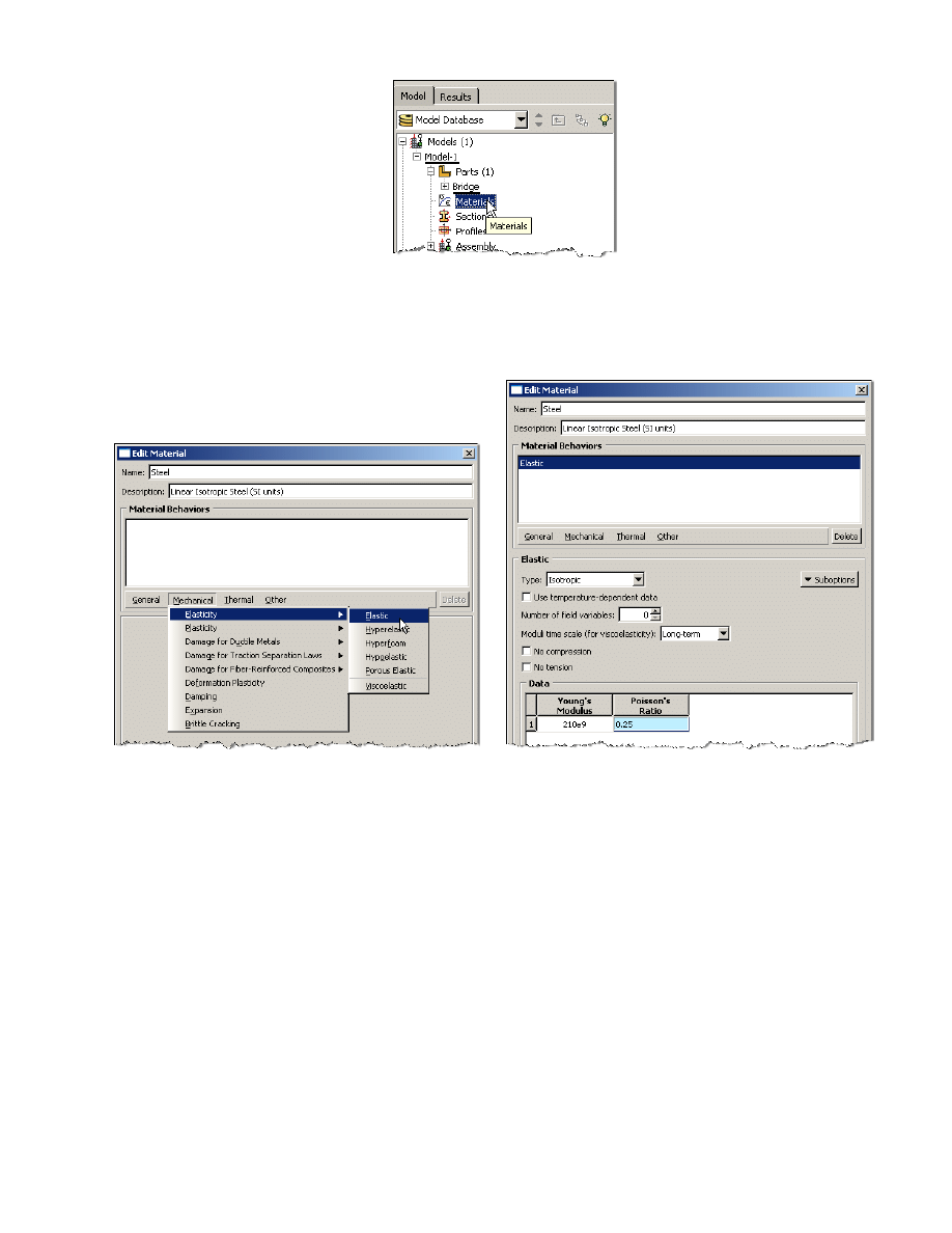
5. Double click on the “Materials” node in the model tree 

 

a. Name the new material and give it a description 
b. Click on the “Mechanical” tabÎElasticityÎElastic 
c. Define Young’s Modulus and Poisson’s Ratio (use SI units) 

i. WARNING:  There are no predefined system of units within Abaqus, so the user is responsible 

for ensuring that the correct values are specified 

 

 

 

d. Click on the “General” tabÎDensity 
e. Density = 7800 
f. Click “OK” 

4 

 

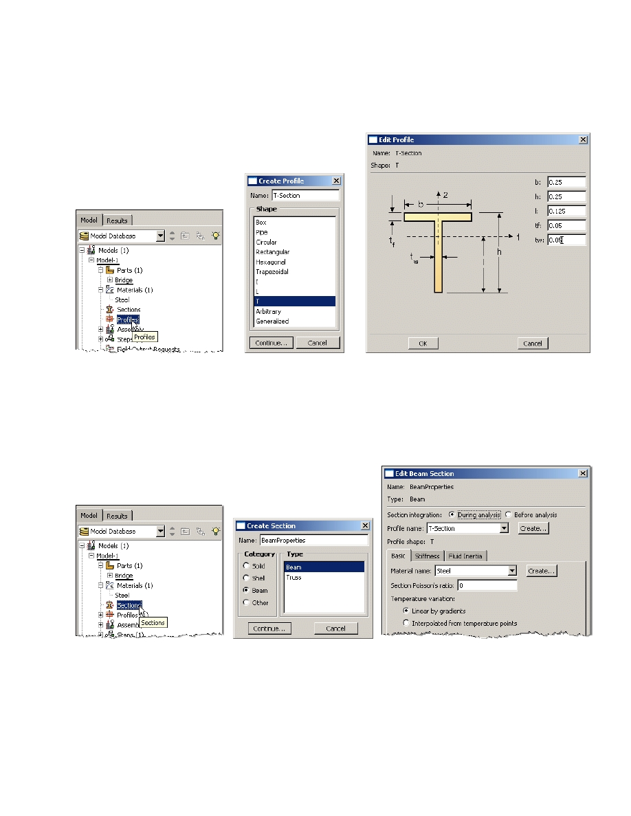
6. Double click on the “Profiles” node in the model tree 

a. Name the profile and select “T” for the shape 

i. Note that the “T” shape is one of several predefined cross‐sections 

b. C lick “Continue…” 
c. Enter the values for the profile shown below 
d. Click “OK” 

        

        

 

7. Double click on the “Sections” node in the model tree 

a. Name the section “BeamProperties” and select “Beam” for both the category and the type 
b. Click “Continue…” 
c. Leave the section integration set to “During Analysis” 
d. Select the profile created above (T‐Section) 
e. Select the material created above (Steel) 
f. Click “OK” 

   

   

 

5 

 

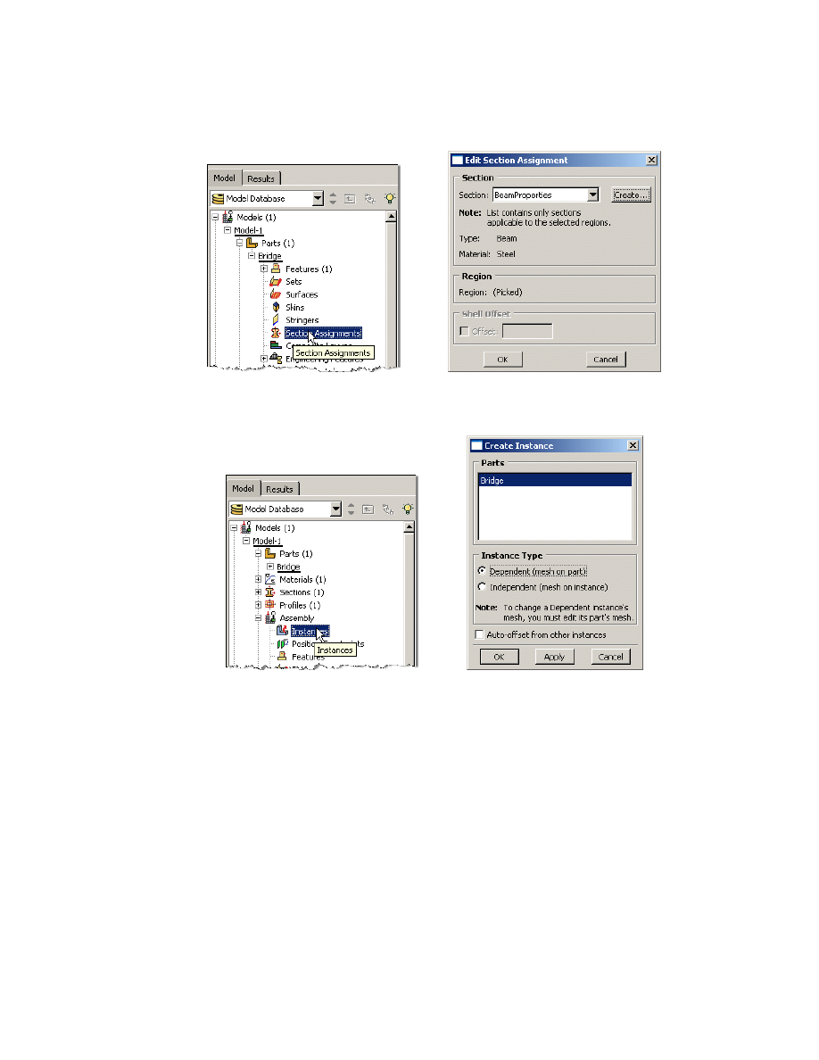
8. Expand the “Parts” node in the model tree, expand the node of the part just created, and double click on 

“Section Assignments” 

a. Select the entire geometry in the viewport 
b. Select the section created above (BeamProperties) 
c. Click “OK” 

 

 

9. Expand the “Assembly” node in the model tree and then double click on “Instances” 

a. Select “Dependent” for the instance type 
b. Click “OK” 

 

 

6 

 

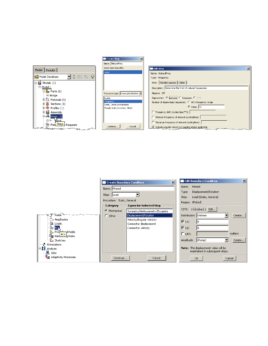
10. Double click on the “Steps” node in the model tree 

a. Name the step, set the procedure to “Linear perturbation”, and select “Frequency” 
b. Click “Continue…” 
c. Give the step a description 
d. Select the radio button “Value” under “Number of eigenvalues requested “ and enter  10 
e. Click “OK” 

     

    

 

11. Double click on the “BCs” node in the model tree 

a. Name the boundary conditioned “Pinned” and select “Displacement/Rotation” for the type 
b. Click “Continue…” 
c. Select the lower‐left vertex of the geometry and press “Done” in the prompt area 
d. Check the U1 and U2 displacements and set them to 0 
e. Click “OK” 

 

 

f. Repeat for the lower‐right vertex, but model a roller restraint (only U2 fixed) instead 

7 

 

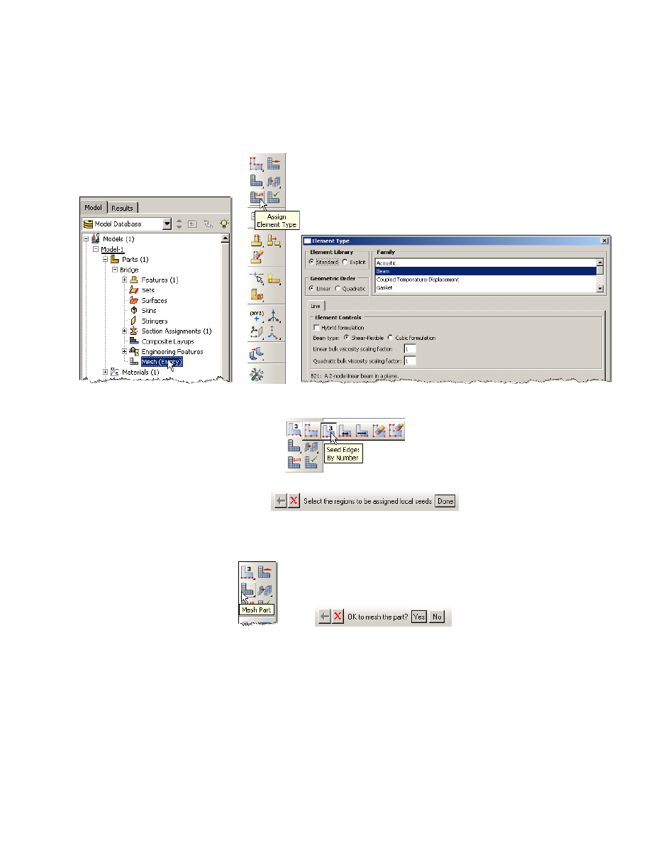
12. In the model tree double click on “Mesh” for the Bridge part, and in the toolbox area click on the “Assign 

Element Type” icon 

a. Select “Standard” for element type 
b. Select “Linear” for geometric order 
c. Select “Beam” for family 
d. Note that the name of the element (B21) and its description are given below the element controls 
e. Click “OK” 

     

 

 

13. In the toolbox area click on the “Seed Edge: By Number” icon (hold down icon to bring up the other options) 

 

a. Select the entire geometry and click “Done” in the prompt area 

 

b. Define the number of elements along the edges as 5 

14. In the toolbox area click on the “Mesh Part” icon 

a. Click “Yes” in the prompt area 

 

 

8 

 

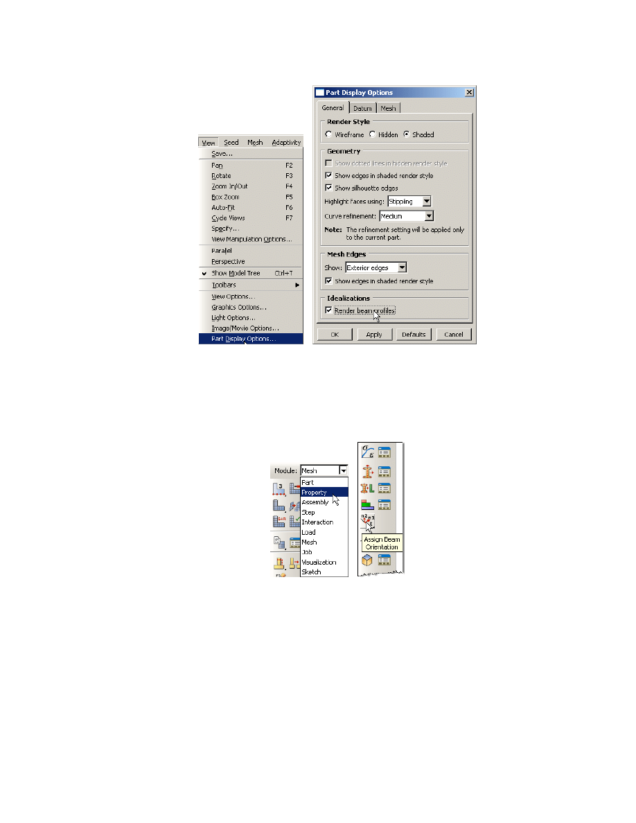
15. In the menu bar select ViewÎPart Display Options 

a. Check the Render beam profiles option 
b. Click “OK” 

   

 

 

16. Change the Module to “Property” 

a. Click on the “Assign Beam Orientation” icon 
b. Select the entire geometry from the viewport 
c. Click “Done” in the prompt area  
d. Accept the default value of the approximate n1 direction 

   

  

 

17. Note that the preview shows that the beam cross sections are not all orientated as desired (see Problem 

Description) 

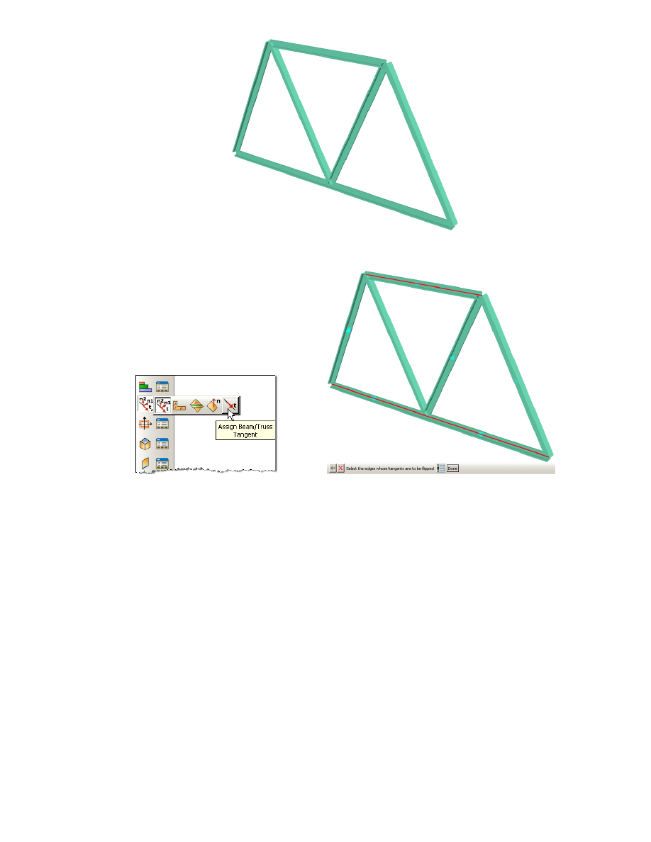
9 

 

 

18. In the toolbox area click on the “Assign Beam/Truss Tangent” icon 

a. Click on the sections of the geometry that are off by 180 degrees 

   

 

 

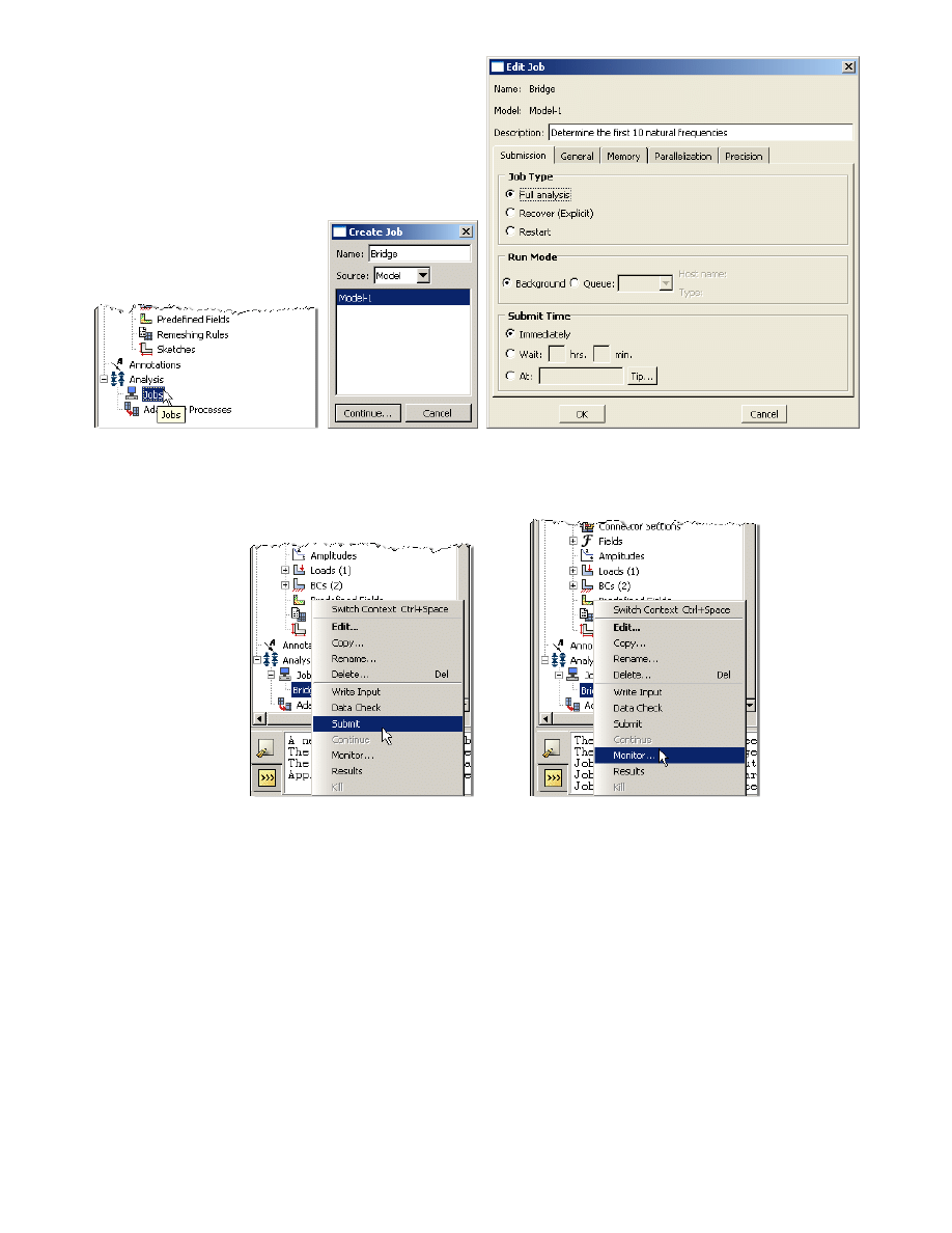
19. In the model tree double click on the “Job” node 

a. Name the job “Bridge” 
b. Click “Continue…” 
c. Give the job a description 
d. Click “OK” 

10 

 

  

 

 

20. In the model tree right click on the job just created (Bridge) and select “Submit” 

a. While Abaqus is solving the problem right click on the job submitted (Bridge), and select “Monitor” 

 

 

 

11 

 

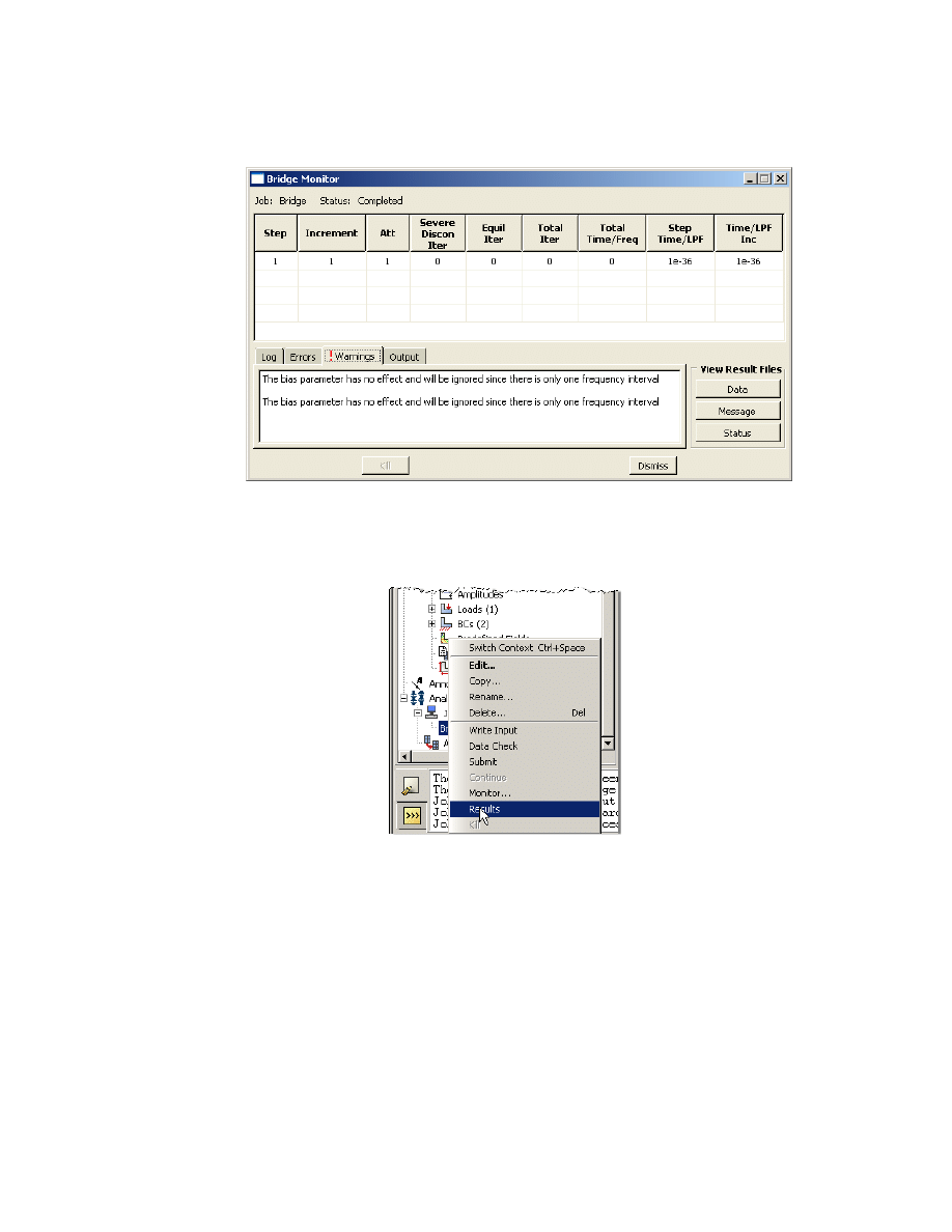
b. In the Monitor window check that there are no errors or warnings 

i. If there are errors, investigate the cause(s) before resolving 

ii. If there are warnings, determine if the warnings are relevant, some warnings can be safely 

ignored 

 

 

21. In the model tree right click on the submitted and successfully completed job (Bridge), and select “Results” 

 

 

12 

 

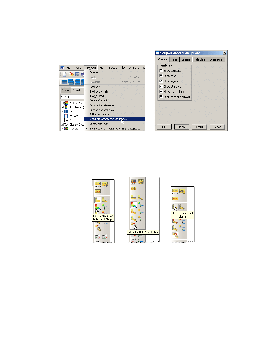
22. In the menu bar click on ViewportÎViewport Annotations Options 

a. Uncheck the “Show compass option” 
b. The locations of viewport items can be specified on the corresponding tab in the Viewport Annotations 

Options 

c. Click “OK” 

 

 

 

23. Display the deformed contour overlaid with the undeformed geometry 

a. In the toolbox area click on the following icons 

i. “Plot Contours on Deformed Shape” 

ii. “Allow Multiple Plot States” 

iii. “Plot Undeformed Shape” 

 

   

 

 

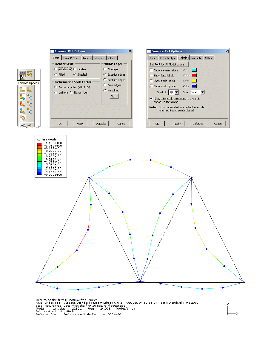
13 

 

24. In the toolbox area click on the “Common Plot Options” icon 

a. Note that the Deformation Scale Factor can be set on the “Basic” tab 
b. On the “Labels” tab check the show node symbols icon 
c. Click “OK” 

  

 

 

14 

 

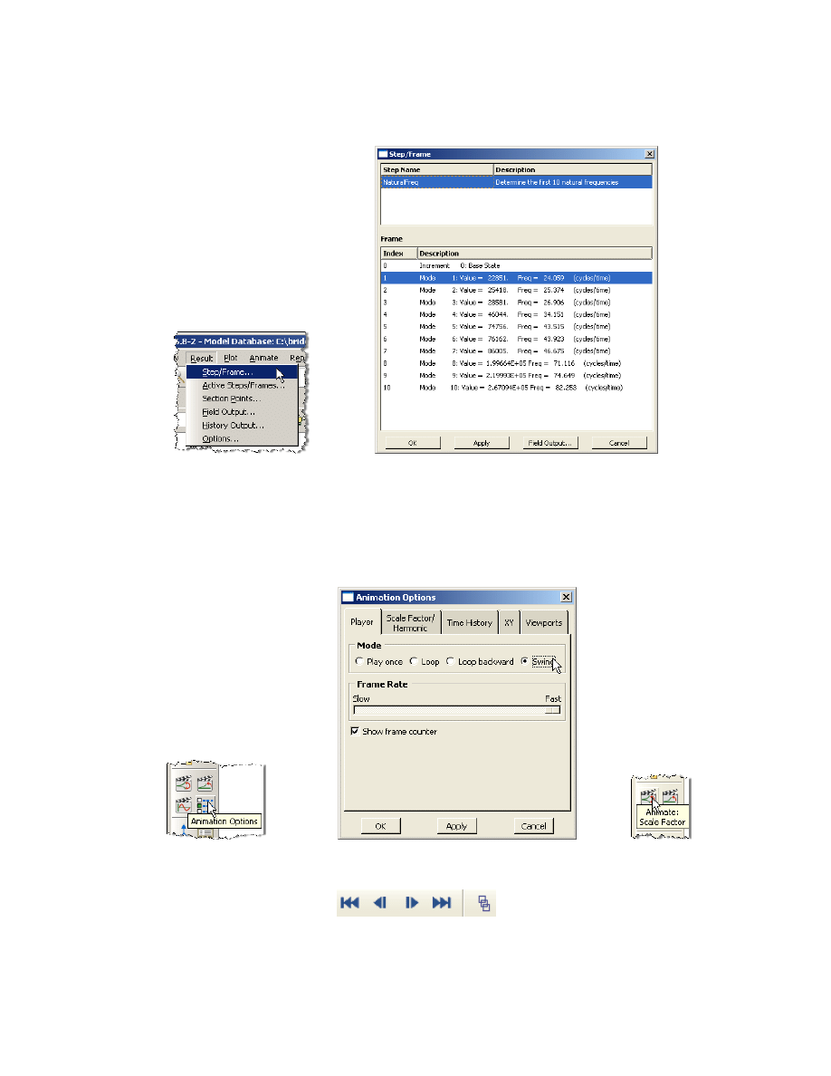
25. In the menu bar click on Results ÎStep/Frame 

a. Change the mode by double clicking in the “Frame” portion of the window 
b. Observe the eigenvalues and frequencies 
c. Click “OK” 

                   

 

26. In the toolbox area click on “Animation Options” 

a. Change the Mode to “Swing” 
b. Click “OK” 
c. Animate by clicking on “Animate:  Scale Factor” icon in the toolbox area 
d. Stop the animation by clicking on the icon again 

 

 

   

 

27. Click on the “Next” arrow on the context bar to change the mode 

 

15 

 

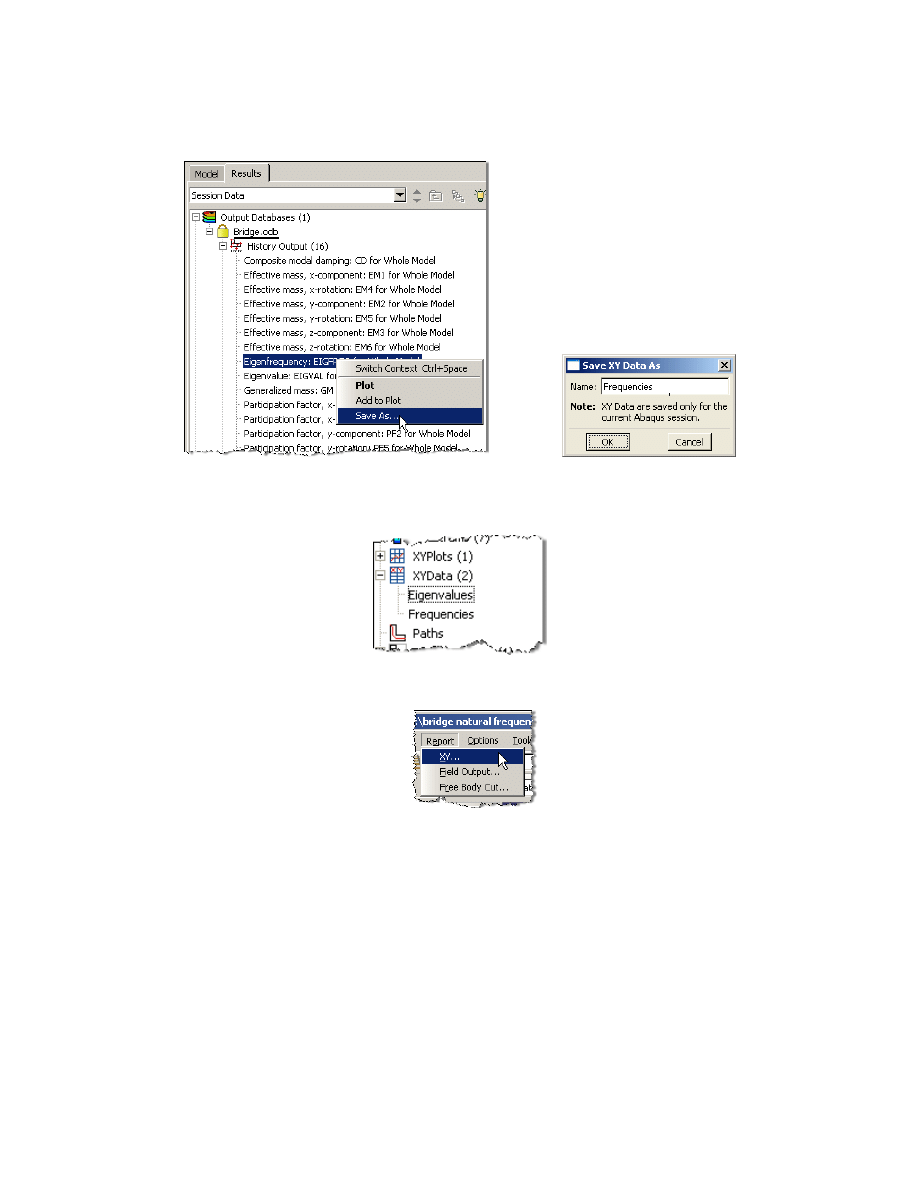
28. Expand the “Bridge.odb” node in the result tree, expand the “History Output” node, and right‐click on 

“Eigenfrequency:  …” 

a. Select “Save As…” 
b. Name = Frequencies 

   

 

c. Repeat for “Eigenvalue” 
d. Observe the XYData nodes in the result tree 

 

29. In the menu bar click on ReportÎXY… 

 

a. Select from = All XY data 
b. Highlight “Eigenvalues” 
c. Click on the “Setup” tab 
d. Click “Select…” and specify the desired name and location of the report 
e. Click “Apply” 
f. Click on the “XY Data” tab 
g. Highlight “Frequencies” 
h. Click “OK” 

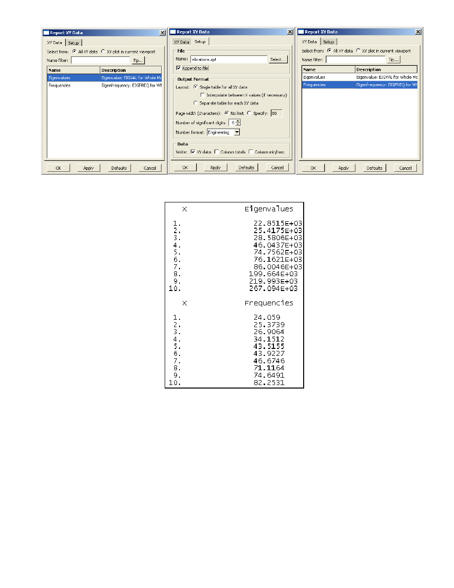
16 

 

 

30. Open the report (.rpt file) with any text editor