Finite Element Method using Pro/ENGINEER and ANSYS

Notes by R.W. Toogood

The transfer of a model from Pro/ENGINEER to ANSYS will be demonstrated here for a simple solid model. Model idealizations
such as shells and beams will not be treated. Also, many modeling options for constraints, loads, mesh control, analysis types will not
be covered. These are fairly easy to figure out once you know the general procedures presented here.

Step 1. Make the part

Use Pro/E to make the part. Things to note are:

z

be aware of your model units

z

note the orientation of the model (default coordinate system in ANSYS will be the same as in Pro/E)

z

IMPORTANT: remove all unnecessary and/or cosmetic features like rounds, chamfers, holes, etc., by suppressing them in
Pro/E. Too much small geometry will cause the mesh generator to create a very fine mesh with many elements which will
greatly increase your solver time. Of course, if the feature is critical to your design, you will want to leave it. You must
compromise between accuracy and available CPU resources.

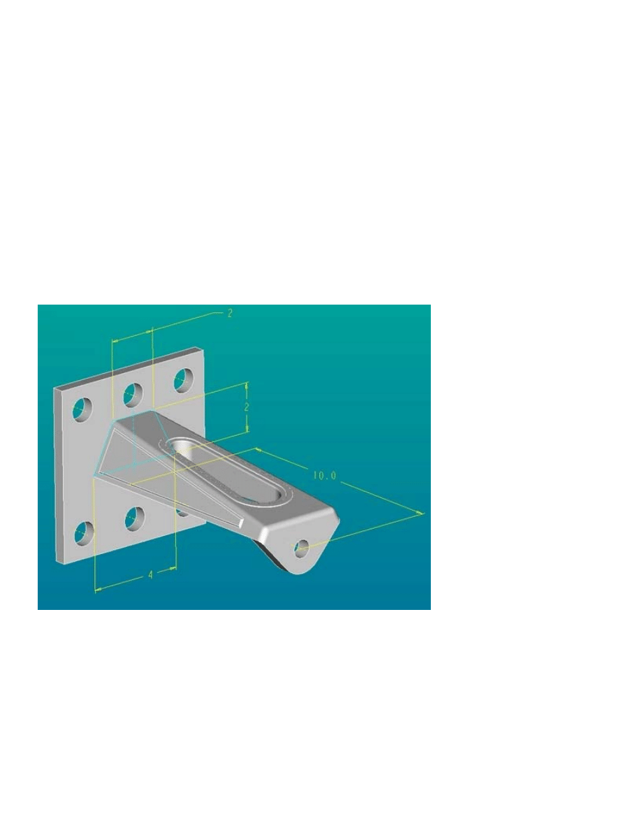
The figure above shows the original model for this demonstration. This is a model of a short cantilevered bracket that bolts to the wall
via the thick plate on the left end. Model units are inches. A load is applied at the hole in the right end. Some cosmetic features are
located on the top surface and the two sides. Several edges are rounded. For this model, the interest is in the stress distribution around
the vertical slot. So, the plate and the loading hole are removed, as are the cosmetic features and rounds resulting in the "de-featured"
geometry shown below. The model will be constrained on the left face and a uniform load will be applied to the right face.

University of Alberta ANSYS Tutorials - www.mece.ualberta.ca/tutorials/ansys/AU/ProE/ProE.html

Copyright © 2001 University of Alberta

Step 2. Create the FEM model

In the pull-down menu at the top of the Pro/E window, select

Applications > Mechanica

An information window opens up to remind you about the units you are using. Press Continue

In the MECHANICA menu at the right, check the box beside FEM Mode and select the command Structure.

A new toolbar appears on the right of the screen that contains icons for creating all the common modeling entities (constraints, loads,
idealizations). All these commands are also available using the command windows that will open on the right side of the screen or in
dialog windows that will open when appropriate.

Notice that a small green coordinate system WCS has appeared. This is how you will specify the directions of constraints and forces.
Other coordinate systems (eg cylindrical) can be created as required and used for the same purpose.

The MEC STRUCT menu appears on the right. Basically, to define the model we proceed down this menu in a top-down manner.
Model is already selected for you which opens the STRC MODEL menu. This is where we specify modeling information. We proceed

in a top-down manner. The Features command allows you to create additional simulation features like datum points, curves, surface
regions, and so on. Idealizations lets you create special modeling entities like shells and beams. The Current CSYS command lets you
create or select an alternate coordinate system for specifying directions of constraints and loads.

Defining Constraints

For our simple model, all we need are constraints, loads, and a specified material. Select

Constraints > New

We can specify constraints on four entity types (basically points, edges, and surfaces). Constraints are organized into constraint sets.
Each constraint set has a unique name (default of the first one is ConstraintSet1) and can contain any number of individual constraints
of different types. Each individual constraint also has a unique name (default of the first one is Constraint1). In the final computed
model, only one set can be included, but this can contain numerous individual constraints.

University of Alberta ANSYS Tutorials - www.mece.ualberta.ca/tutorials/ansys/AU/ProE/ProE.html

Copyright © 2001 University of Alberta

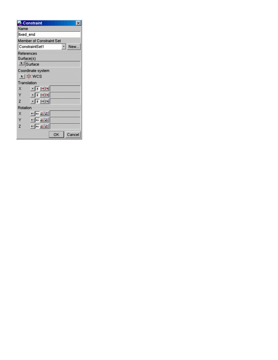
Select Surface. We are going to fully constrain the left face of the cantilever. A dialog window opens as shown above. Here you can

give a name to the constraint and identify which constraint set it belongs to. Since we elected to create a surface constraint, we now
select the surface we want constrained (push the Surface selection button in the window and then click on the desired surface of the

model). The constraints to be applied are selected using the buttons at the bottom of the window. In general we specify constraints on
translation and rotation for any mesh node that will appear on the selected entity. For each direction X, Y, and Z, we can select one of
the four buttons (Free, Fixed, Prescribed, and Function of Coordinates). For our solid model, the rotation constraints are irrelevant

(since nodes of solid elements do not have this degree of freedom anyway). For beams and shells, rotational constraints are active if
specified.

For our model, leave all the translation constraints as FIXED, and select the OK button. You should now see some orange symbols on

the left face of the model, along with some text labels that summarize the constraint settings.

Defining Loads

In the STRC MODEL menu select

Loads > New > Surface

University of Alberta ANSYS Tutorials - www.mece.ualberta.ca/tutorials/ansys/AU/ProE/ProE.html

Copyright © 2001 University of Alberta

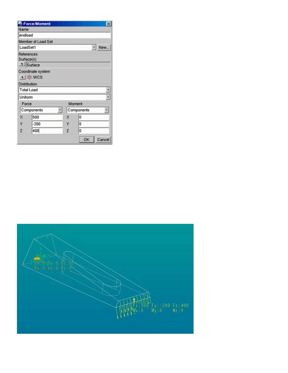
The FORCE/MOMENT window opens as shown above. Loads are also organized into named load sets. A load set can contain any
number of individual loads of different types. A FEM model can contain any number of different load sets. For example, in the
analysis of a pressurized tank on a support system with a number of nozzle connections to other pipes, one load set might contain only
the internal pressure, another might contain the support forces, another a temperature load, and more might contain the forces applied
at each nozzle location. These can be solved at the same time, and the principle of superposition used to combine them in numerous
ways.

Create a load called "end_load" in the default load set (LoadSet1)

Click on the Surfaces button, then select the right face of the model and middle click to return to this dialog. Leave the defaults for the

load distribution. Enter the force components at the bottom. Note these are relative to the WCS. Then select OK. The load should be

displayed symbolically as shown in the figure below.

Note that constraint and load sets appear in the model tree. You can select and edit these in the usual way using the right mouse
button.

University of Alberta ANSYS Tutorials - www.mece.ualberta.ca/tutorials/ansys/AU/ProE/ProE.html

Copyright © 2001 University of Alberta

Assigning Materials

Our last job to define the model is to specify the part material. In the STRC MODEL menu, select

Materials > Whole Part

In the library dialog window, select a material and move it to the right pane using the triple arrow button in the center of the window.
In an assembly, you could now assign this material to individual parts. If you select the Edit button, you will see the properties of the
chosen material.

At this point, our model has the necessary information for solution (constraints, loads, material).

Step 3. Define the analysis

Select

Analyses > New

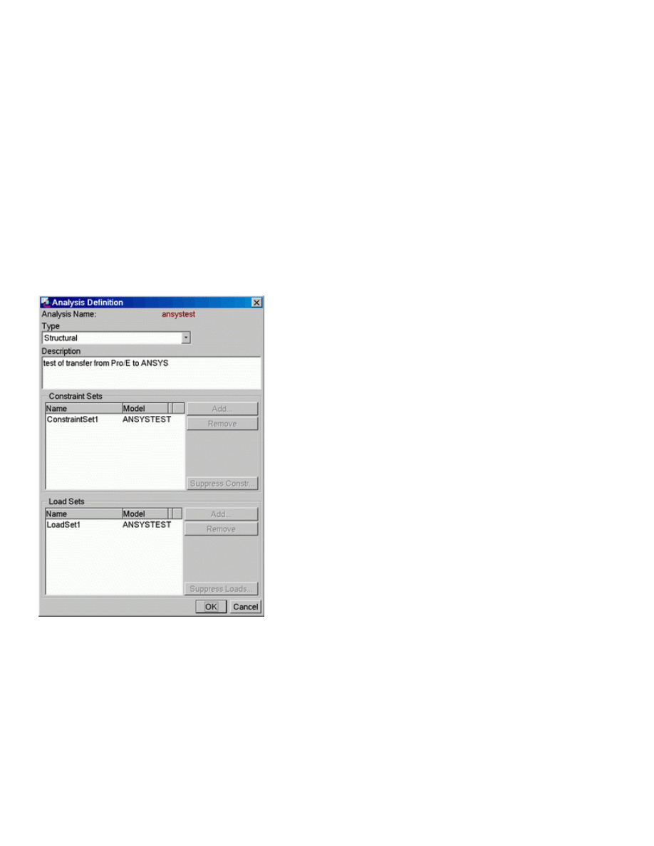
Specify a name for the analysis, like "ansystest". Select the type (Structural or Modal). Enter a short description. Now select the Add
buttons beside the Constraints and Loads panes to add ConstraintSet1 and LoadSet1 to the analysis. Now select OK.

Step 4. Creating the mesh

We are going to use defaults for all operations here. The MEC STRUCT window, select

Mesh > Create > Solid > Start

Accept the default for the global minimum. The mesh is created and another dialog window opens (Element Quality Checks).

University of Alberta ANSYS Tutorials - www.mece.ualberta.ca/tutorials/ansys/AU/ProE/ProE.html

Copyright © 2001 University of Alberta

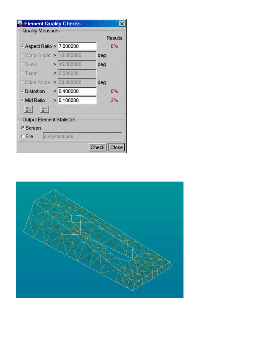
This indicates some aspects of mesh quality that may be specified and then, by selecting the Check button at the bottom, evaluated for

the model. The results are indicated in columns on the right. If the mesh does not pass these quality checks, you may want to go back
to specify mesh controls (discussed below). Select Close. Here is an image of the default mesh, shown in wire frame.

Improving the Mesh

In the mesh command, you can select the Controls option. This will allow you to select points, edges, and surfaces where you want to
specify mesh geometry such as hard points, maximum mesh size, and so on. Beware that excessively tight mesh controls can result in
meshes with many elements.

University of Alberta ANSYS Tutorials - www.mece.ualberta.ca/tutorials/ansys/AU/ProE/ProE.html

Copyright © 2001 University of Alberta

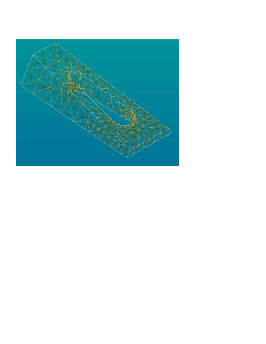
For example, setting a maximum mesh size along the curved ends of the slot results in the following mesh. Notice the better
representation of the curved edges than in the previous figure. This is at the expense of more than double the number of elements.
Note that mesh controls are also added to the model tree.

Step 5. Creating the Output file

All necessary aspects of the model are now created (constraints, loads, materials, mesh). In the MEC STRUCT menu, select

Run

University of Alberta ANSYS Tutorials - www.mece.ualberta.ca/tutorials/ansys/AU/ProE/ProE.html

Copyright © 2001 University of Alberta

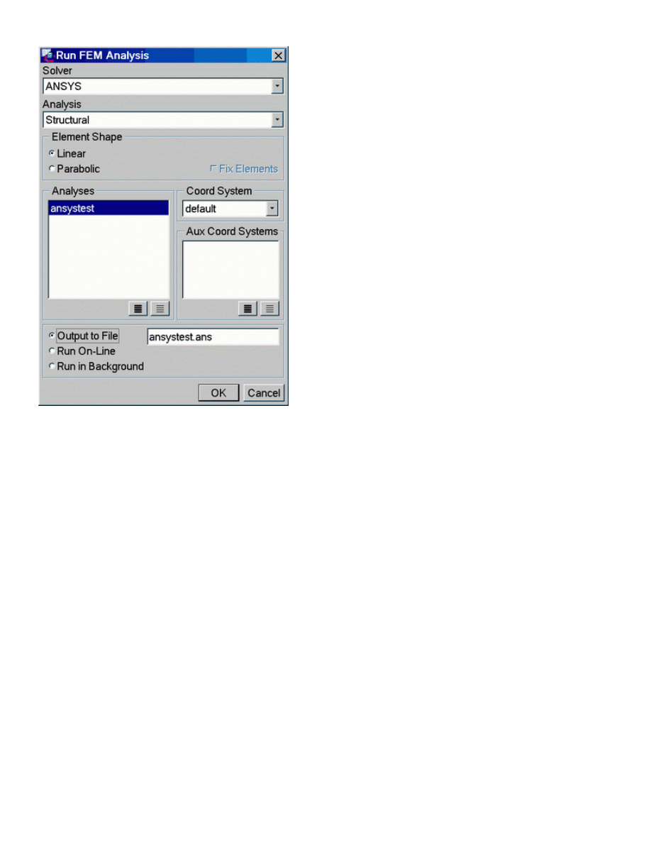
This opens the Run FEM Analysis dialog window shown here. In the Solver pull-down list at the top, select ANSYS. In the Analysis

list, select Structural. You pick either Linear or Parabolic elements. The analysis we defined (containing constraints, loads, mesh, and

material) is listed. Select the Output to File radio button at the bottom and specify the output file name (default is the analysis name

with extension .ans). Select OK and read the message window.

We are now finished with Pro/E. Go to the top pull-down menus and select

Applications > Standard

Save the model file and leave the program.

Copy the .ans file from your Pro/E working directory to the directory you will use for running ANSYS.

Step 6. Importing into ANSYS

Launch ANSYS Interactive and select

File > Read Input From...

Select the .ans file you created previously. This will read in the entire model. You can display the model using (in the pull down
menus) Plot > Elements.

Step 7. Running the ANSYS solver

In the ANSYS Main Menu on the left, select

Solution > Solve > Current LS > OK

University of Alberta ANSYS Tutorials - www.mece.ualberta.ca/tutorials/ansys/AU/ProE/ProE.html

Copyright © 2001 University of Alberta

After a few seconds, you will be informed that the solution is complete.

Step 8. Viewing the results

There are myriad possibilities for viewing FEM results. A common one is the following:

General Postproc > Plot Results > Contour Plot > Nodal Solu

Pick the Von Mises stress values, and select Apply. You should now have a color fringe plot of the Von Mises stress displayed on the
model.

Updated: 8 November 2002 using Pro/ENGINEER 2001
RWT
Please report errors or omissions to

Roger Toogood

University of Alberta ANSYS Tutorials - www.mece.ualberta.ca/tutorials/ansys/AU/ProE/ProE.html

Copyright © 2001 University of Alberta