Comparing Images Using Color Coherence Vectors

Greg Pass

Ramin Zabih

∗

Justin Miller

Computer Science Department

Cornell University

Ithaca, NY 14853

gregpass,rdz,[e-mail]

http://www.cs.cornell.edu/home/rdz/ccv.html

Abstract

Color histograms are used to compare images
in many applications. Their advantages are ef-
ficiency, and insensitivity to small changes in
camera viewpoint. However, color histograms
lack spatial information, so images with very
different appearances can have similar his-
tograms.

For example, a picture of fall fo-

liage might contain a large number of scattered
red pixels; this could have a similar color his-
togram to a picture with a single large red ob-
ject. We describe a histogram-based method
for comparing images that incorporates spa-
tial information. We classify each pixel in a
given color bucket as either coherent or inco-
herent, based on whether or not it is part of a
large similarly-colored region. A color coher-
ence vector (CCV) stores the number of coher-
ent versus incoherent pixels with each color.
By separating coherent pixels from incoherent
pixels, CCV’s provide finer distinctions than
color histograms. CCV’s can be computed at
over 5 images per second on a standard work-
station. A database with 15,000 images can
be queried for the images with the most sim-
ilar CCV’s in under 2 seconds. We show that
CCV’s can give superior results to color his-

∗

To whom correspondence should be addressed

tograms for image retrieval.

KEYWORDS: Content-based Image Re-
trieval, Processing, Color Histograms

INTRODUCTION

Many applications require simple methods for
comparing pairs of images based on their over-
all appearance. For example, a user may wish
to retrieve all images similar to a given im-
age from a large database of images. Color
histograms are a popular solution to this prob-
lem, and are used in systems like QBIC [4] and
Chabot [11]. Color histograms are computa-
tionally efficient, and generally insensitive to
small changes in camera position.

Color histograms also have some limita-

tions. A color histogram provides no spatial
information; it merely describes which colors
are present in the image, and in what quanti-
ties. In addition, color histograms are sensitive
to both compression artifacts and changes in
overall image brightness.

In this paper we describe a color-based

method for comparing images which is similar
to color histograms, but which also takes spa-
tial information into account. We begin with a

1

review of color histograms. We then describe
color coherence vectors (CCV’s) and how to
compare them. Examples of CCV-based im-
age queries demonstrate that they can give
superior results to color histograms. We con-
trast our method with some recent algorithms
[8, 14, 15, 17] that also combine spatial in-
formation with color histograms. Finally, we
present some possible extensions to CCV’s.

COLOR HISTOGRAMS

Color histograms are frequently used to com-
pare images. Examples of their use in multi-
media applications include scene break detec-
tion [1, 7, 10, 12, 22] and querying a database
of images [3, 4, 11, 13]. Their popularity stems
from several factors.

• Color histograms are computationally

trivial to compute.

• Small changes in camera viewpoint tend

not to effect color histograms.

• Different objects often have distinctive

color histograms.

Researchers in computer vision have also

investigated color histograms.

For exam-

ple, Swain and Ballard [19] describe the use
of color histograms for identifying objects.
Hafner et al. [6] provide an efficient method
for weighted-distance indexing of color his-
tograms. Stricker and Swain [18] analyze the
information capacity of color histograms, as
well as their sensitivity.

Definitions

We will assume that all images are scaled to
contain the same number of pixels M . We dis-
cretize the colorspace of the image such that
there are n distinct (discretized) colors. A

color histogram H is a vector hh

1

, h

2

, . . . , h

n

i,

in which each bucket h

j

contains the number

of pixels of color j in the image. Typically im-
ages are represented in the RGB colorspace,
and a few of the most significant bits are used
from each color channel. For example, Zhang
[22] uses the 2 most significant bits of each
color channel, for a total of n = 64 buckets in
the histogram.

For a given image I, the color histogram

H

I

is a compact summary of the image. A

database of images can be queried to find
the most similar image to I, and can return
the image I

0

with the most similar color his-

togram H

I

0

. Typically color histograms are

compared using the sum of squared differences
(L

2

-distance) or the sum of absolute value of

differences (L

1

-distance). So the most similar

image to I would be the image I

0

minimizing

kH

I

− H

I

0

k =

n

X

j=1

(H

I

[j] − H

I

0

[j])

2

,

for the L

2

-distance, or

|H

I

− H

I

0

| =

n

X

j=1

|H

I

[j] − H

I

0

[j]|,

for the L

1

-distance. Note that we are assum-

ing that differences are weighted evenly across
different color buckets for simplicity.

COLOR

COHERENCE

VECTORS

Intuitively, we define a color’s coherence as the
degree to which pixels of that color are mem-
bers of large similarly-colored regions. We re-
fer to these significant regions as coherent re-
gions, and observe that they are of significant
importance in characterizing images.

2

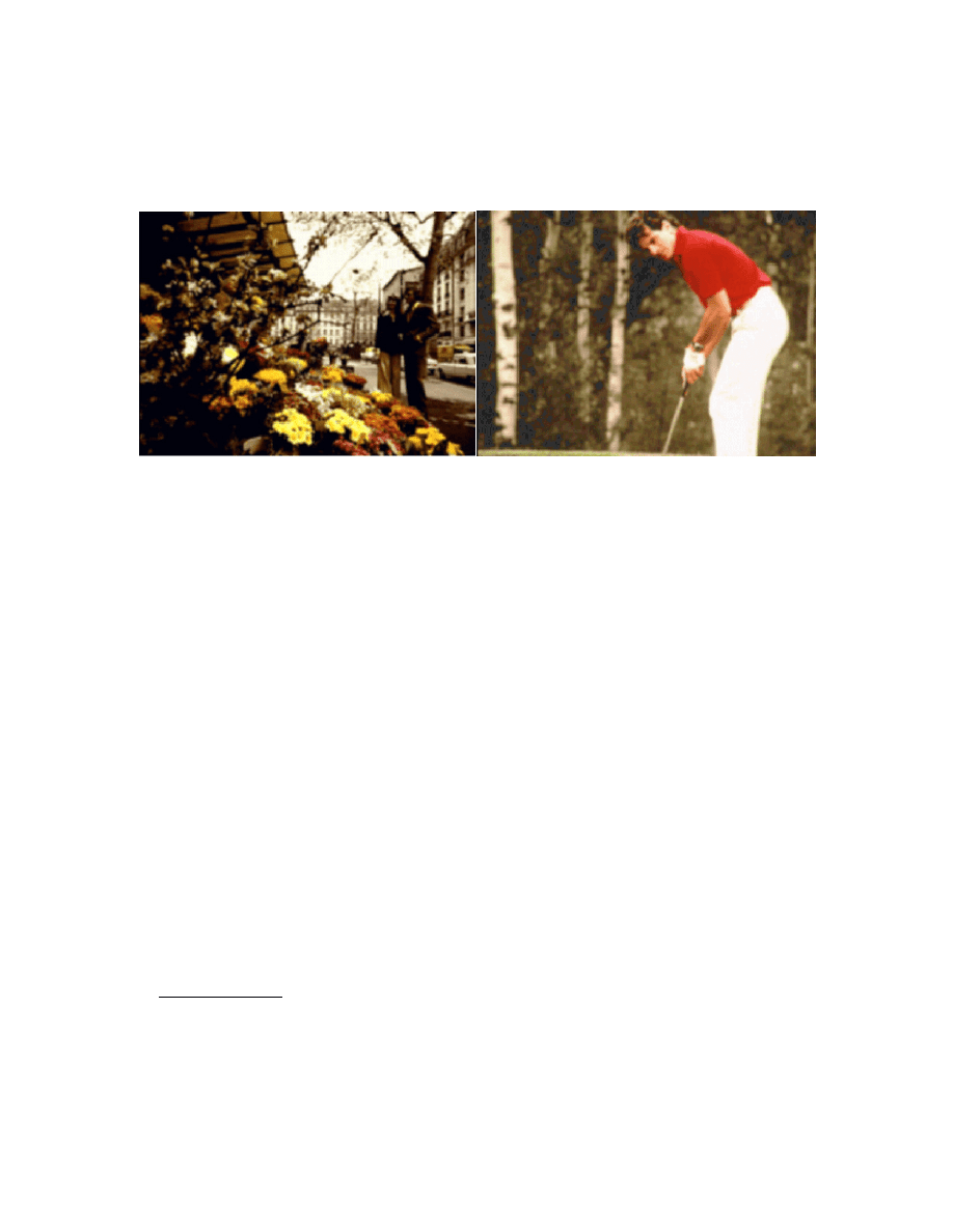
Figure 1: Two images with similar color histograms

For example, the images shown in figure 1

have similar color histograms, despite their
rather different appearances.

1

The color red

appears in both images in approximately the
same quantities.

In the left image the red

pixels (from the flowers) are widely scattered,
while in the right image the red pixels (from
the golfer’s shirt) form a single coherent re-
gion.

Our coherence measure classifies pixels as

either coherent or incoherent. Coherent pixels
are a part of some sizable contiguous region,
while incoherent pixels are not. A color co-
herence vector represents this classification for
each color in the image. CCV’s prevent co-
herent pixels in one image from matching in-
coherent pixels in another. This allows fine
distinctions that cannot be made with color
histograms.

Computing CCV’s

The initial stage in computing a CCV is sim-
ilar to the computation of a color histogram.
We first blur the image slightly by replacing

1

The color images used in this paper can be found

at http://www.cs.cornell.edu/home/rdz/ccv.html.

pixel values with the average value in a small
local neighborhood (currently including the 8
adjacent pixels). This eliminates small vari-
ations between neighboring pixels. We then
discretize the colorspace, such that there are
only n distinct colors in the image.

The next step is to classify the pixels within

a given color bucket as either coherent or in-
coherent. A coherent pixel is part of a large
group of pixels of the same color, while an in-
coherent pixel is not. We determine the pixel
groups by computing connected components.
A connected component C is a maximal set of
pixels such that for any two pixels p, p

0

∈ C,

there is a path in C between p and p

0

. (For-

mally, a path in C is a sequence of pixels
p = p

1

, p

2

, . . . , p

n

= p

0

such that each pixel p

i

is in C and any two sequential pixels p

i

, p

i+1

are adjacent to each other. We consider two
pixels to be adjacent if one pixel is among the
eight closest neighbors of the other; in other
words, we include diagonal neighbors.) Note
that we only compute connected components
within a given discretized color bucket. This
effectively segments the image based on the
discretized colorspace.

Connected components can be computed in

3

linear time (see, for example, [20]). When this
is complete, each pixel will belong to exactly
one connected component. We classify pixels
as either coherent or incoherent depending on
the size in pixels of its connected component.
A pixel is coherent if the size of its connected
component exceeds a fixed value τ ; otherwise,
the pixel is incoherent.

For a given discretized color, some of the

pixels with that color will be coherent and
some will be incoherent. Let us call the num-
ber of coherent pixels of the j’th discretized
color α

j

and the number of incoherent pixels

β

j

. Clearly, the total number of pixels with

that color is α

j

+ β

j

, and so a color histogram

would summarize an image as

hα

1

+ β

1

, . . . , α

n

+ β

n

i .

Instead, for each color we compute the pair

(α

j

, β

j

)

which we will call the coherence pair for the
j’th color. The color coherence vector for the
image consists of

h(α

1

, β

1

) , . . . , (α

n

, β

n

)

i .

This is a vector of coherence pairs, one for each
discretized color.

In our experiments, all images were scaled

to contain M = 38, 976 pixels, and we have
used τ = 300 pixels (so a region is classified
as coherent if its area is about 1% of the im-
age). With this value of τ , an average image
in our database consists of approximately 75%
coherent pixels.

An example CCV

We next demonstrate the computation of a
CCV. To keep our example small, we will let
τ = 4 and assume that we are dealing with an
image in which all 3 color components have

the same value at every pixel (in the RGB col-
orspace this would represent a grayscale im-
age).

This allows us to represent a pixel’s

color with a single number (i.e., the pixel with
R/G/B values 12/12/12 will be written as 12).

Suppose that after we slightly blur the input

image, the resulting intensities are as follows.

22

10

21

22

15

16

24

21

13

20

14

17

23

17

38

23

17

16

25

25

22

14

15

21

27

22

12

11

21

20

24

21

10

12

22

23

Let us discretize the colorspace so that bucket
1 contains intensities 10 through 19, bucket 2
contains 20 through 29, etc. Then after dis-
cretization we obtain

2

1

2

2

1

1

2

2

1

2

1

1

2

1

3

2

1

1

2

2

2

1

1

2

2

2

1

1

2

2

2

2

1

1

2

2

The next step is to compute the connected
components.

Individual components will be

labeled with letters (A, B, . . .) and we will
need to keep a table which maintains the dis-
cretized color associated with each label, along
with the number of pixels with that label. Of
course, the same discretized color can be asso-
ciated with different labels if multiple contigu-
ous regions of the same color exist. The image
may then become

B

C

B

B

A

A

B

B

C

B

A

A

B

C

D B

A

A

B

B

B

A

A E

B

B

A

A E

E

B

B

A

A E

E

and the connected components table will be

4

Label

A

B

C

D

E

Color

1

2

1

3

1

Size

12

15

3

1

5

The components A, B, and E have more than
τ pixels, and the components C and D less
than τ pixels. Therefore the pixels in A, B and
E are classified as coherent, while the pixels in
C and D are classified as incoherent.

The CCV for this image will be

Color

1

2

3

α

17

15

0

β

3

0

1

A given color bucket may thus contain only co-
herent pixels (as does 2), only incoherent pix-
els (as does 3), or a mixture of coherent and
incoherent pixels (as does 1). If we assume
there are only 3 possible discretized colors, the
CCV can also be written

h(17, 3) , (15, 0) , (0, 1)i .

Comparing CCV’s

Consider two images I and I

0

, together with

their CCV’s G

I

and G

I

0

, and let the number

of coherent pixels in color bucket j be α

j

(for

I) and α

0

j

(for I

0

). Similarly, let the number

of incoherent pixels be β

j

and β

0

j

. So

G

I

=

h(α

1

, β

1

) , . . . , (α

n

, β

n

)

i

and

G

I

0

=

h(α

0

1

, β

0

1

) , . . . , (α

0

n

, β

0

n

)

i

Color histograms will compute the difference
between I and I

0

as

∆

H

=

n

X

j=1



(α

j

+ β

j

)

− (α

0

j

+ β

0

j

)



.

(1)

Our method for comparing is based on the
quantity

∆

G

=

n

X

j=1



(α

j

− α

0

j

)



+



(β

j

− β

0

j

)



. (2)

From equations 1 and 2, it follows that
CCV’s create a finer distinction than color his-
tograms. A given color bucket j can contain
the same number of pixels in I as in I

0

, i.e.

α

j

+ β

j

=

α

0

j

+ β

0

j

,

but these pixels may be entirely coherent in
I and entirely incoherent in I

0

. In this case

β

j

= α

0

j

= 0, and while ∆

H

= 0, ∆

G

will be

large.

In general, ∆

H

≤ ∆

G

. This is true even

if we use squared differences instead of abso-
lute differences in the definitions of ∆

H

and

∆

G

.

This is because both d(x) = |x| and

d(x) = x

2

are metrics, so they satisfy the tri-

angle inequality

d(x + y)

≤ d(x) + d(y).

(3)

If we rearrange the terms in equation 1 we get

∆

H

=

n

X

j=1



(α

j

− α

0

j

) + (β

j

− β

0

j

)



.

Applying the triangle inequality we have

∆

H

≤

n

X

j=1



(α

j

− α

0

j

)



+



(β

j

− β

0

j

)



=

∆

G

.

EXPERIMENTAL

RESULTS

We have implemented color coherence vectors,
and have used them for image retrieval from
a large database.

Our database consists of

14,554 images, which are drawn from a vari-
ety of sources. Our largest sources include the
11,667 images used in Chabot [11], the 1,440
images used in QBIC [4], and a 1,005 image
database available from Corel. In addition, we
included a few groups of images in PhotoCD
format. Finally, we have taken a number of
MPEG videos from the Web and segmented

5

them into scenes using the method described
in [21].

We have added one or two images

from each scene to the database, totaling 349
images. The image database thus contains a
wide variety of imagery. In addition, some of
the imagery has undergone substantial lossy
compression via JPEG or MPEG.

We have compared our results with a num-

ber of color histogram variations. These in-
clude the L

1

and L

2

distances, with both 64

and 512 color buckets. In addition, we have
implemented Swain’s opponent axis colorspace
[19], and used the color discretization scheme
he describes. In each case we include a small
amount of smoothing as it improves the perfor-
mance of color histograms. On our database,
the L

1

distance with the 64-bucket RGB col-

orspace gave the best results, and is used as a
benchmark against CCV’s.

Hand examination of our database re-

vealed 52 pairs of images which contain dif-
ferent views of the same scene.

Examples

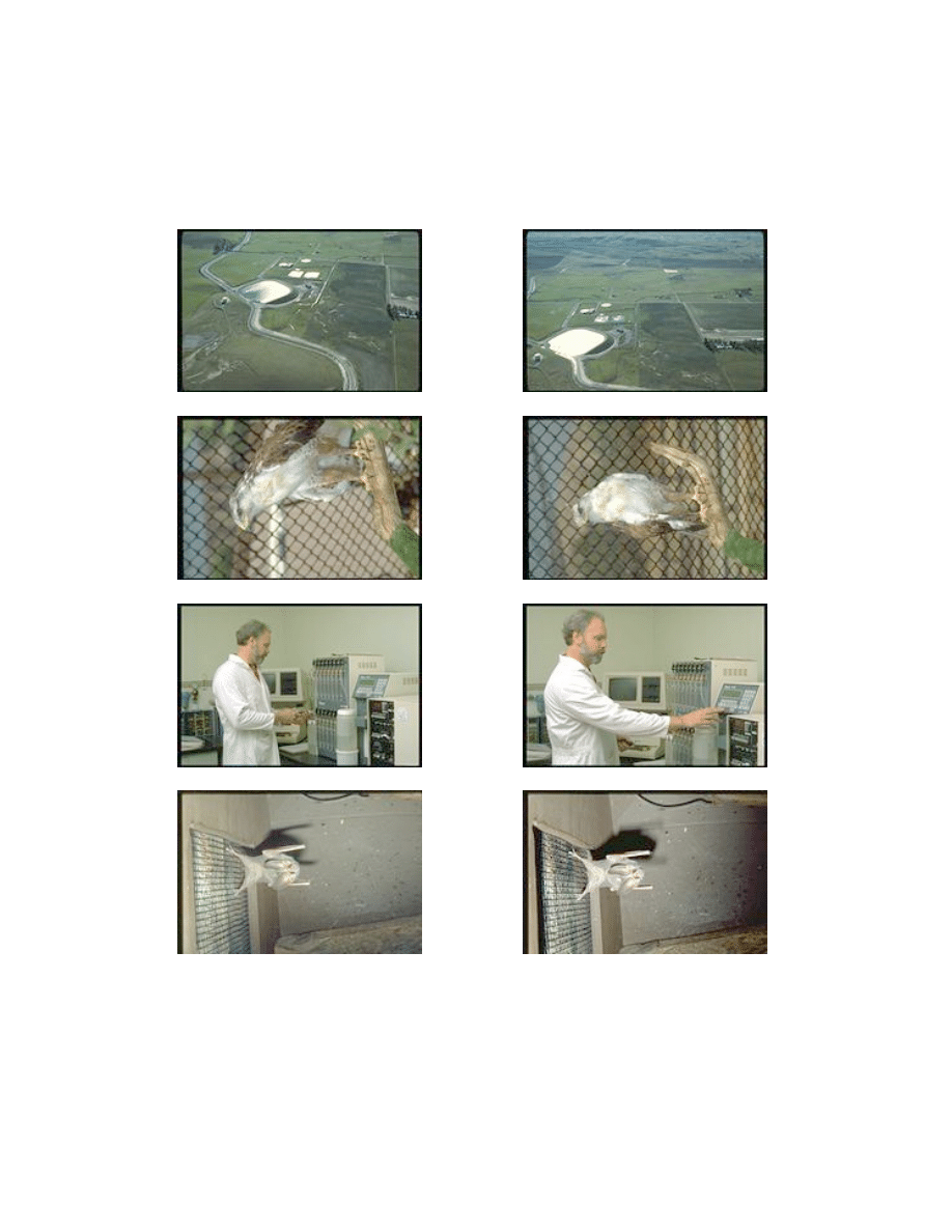
are shown in figures 3 and 4.

One im-

age is selected as a query image, and the
other represents a “correct” answer.

In

each case, we have shown where the sec-
ond image ranks, when similarity is com-
puted using color histograms versus CCV’s.
The color images shown are available at
http://www.cs.cornell.edu/home/rdz/ccv.html.

In 46 of the 52 cases, CCV’s produced better

results, while in 6 cases they produced worse
results. The average change in rank due to
CCV’s was an improvement of just over 75
positions (note that this included the 6 cases
where CCV’s do worse). The average percent-
age change in rank was an improvement of
30%. In the 46 cases where CCV’s performed
better than color histograms, the average im-
provement in rank was 88 positions, and the
average percentage improvement was 50%. In
the 6 cases where color histograms performed
better than CCV’s, the average rank improve-
ment was 21 positions, and the average per-

centage improvement was 48%. A histogram
of the change in rank obtained by using CCV’s
is shown in figure 2.

When CCV’s produced worse results, it was

always due to a change in overall image bright-
ness (i.e., the two images were almost iden-
tical, except that one was brighter than the
other). Because CCV’s use discretized color
buckets for segmentation, they are more sen-
sitive to changes in overall image brightness
than color histograms. We believe that this
difficulty can be overcome by using a better
colorspace than RGB, as we discuss in the ex-
tensions section of this paper.

Efficiency

There are two phases to the computation in-
volved in querying an image database. First,
when an image is inserted into the database,
a CCV must be computed. Second, when the
database is queried, some number of the most
similar images must be retrieved. Most meth-
ods for content-based indexing include these
distinct phases. For both color histograms and
CCV’s, these phases can be implemented in
linear time.

We ran our experiments on a 50 MHz

SPARCstation 20, and provide the results
from color histogramming for comparison.
Color histograms can be computed at 67 im-
ages per second, while CCV’s can be com-
puted at 5 images per second.

Using color

histograms, 21,940 comparisons can be per-
formed per second, while with CCV’s 7,746
can be performed per second.

The images

used for benchmarking are 232

× 168. Both

implementations are preliminary, and the per-
formance can definitely be improved.

6

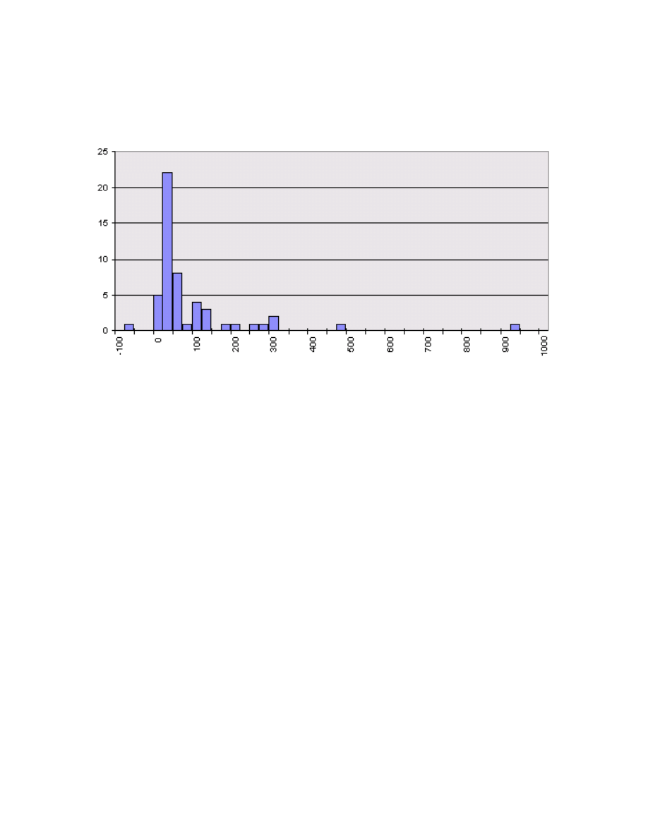
Figure 2: Change in rank due to CCV’s. Positive numbers indicate improved performance.

RELATED WORK

Recently, several authors have proposed al-
gorithms for comparing images that com-
bine spatial information with color histograms.
Hsu et al. [8] attempts to capture the spa-
tial arrangement of the different colors in the
image, in order to perform more accurate
content-based image retrieval. Rickman and
Stonham [14] randomly sample the endpoints
of small triangles and compare the distribu-
tions of these triplets. Smith and Chang [15]
concentrate on queries that combine spatial in-
formation with color. Stricker and Dimai [17]
divide the image into five partially overlapping
regions and compute the first three moments
of the color distributions in each image. We
will discuss each approach in turn.

Hsu [8] begins by selecting a set of repre-

sentative colors from the image.

Next, the

image is partitioned into rectangular regions,
where each region is predominantly a single

color. The partitioning algorithm makes use
of maximum entropy. The similarity between
two images is the degree of overlap between
regions of the same color. Hsu presents re-
sults from querying a database with 260 im-
ages, which show that the integrated approach
can give better results than color histograms.

While the authors do not report running

times, it appears that Hsu’s method requires
substantially more computation than the ap-
proach we describe.

A CCV can be com-

puted in a single pass over the image, with a
small number of operations per pixel. Hsu’s
partitioning algorithm in particular appears
much more computationally intensive than our
method. Hsu’s approach can be extended to
be independent of orientation and position,
but the computation involved is quite substan-
tial. In contrast, our method is naturally in-
variant to orientation and position.

Rickman and Stonham [14] randomly sam-

ple pixel triples arranged in an equilateral tri-

7

Histogram rank: 50. CCV rank: 26.

Histogram rank: 35. CCV rank: 9.

Histogram rank: 367. CCV rank: 244.

Histogram rank: 128. CCV rank: 32.

Figure 3: Example queries with their partner images

8

Histogram rank: 310. CCV rank: 205.

Histogram rank: 88. CCV rank: 38.

Histogram rank: 13. CCV rank: 5.

Histogram rank: 119. CCV rank: 43.

Figure 4: Additional examples

9

angle with a fixed side length. They use 16
levels of color hue, with non-uniform quanti-
zation. Approximately a quarter of the pixels
are selected for sampling, and their method
stores 372 bits per image. They report results
from a database of 100 images.

Smith and Chang’s algorithm also partitions

the image into regions, but their approach is
more elaborate than Hsu’s. They allow a re-
gion to contain multiple different colors, and
permit a given pixel to belong to several differ-
ent regions. Their computation makes use of
histogram back-projection [19] to back-project
sets of colors onto the image. They then iden-
tify color sets with large connected compo-
nents.

Smith and Chang’s image database contains

3,100 images. Again, running times are not
reported, although their algorithm does speed
up back-projection queries by pre-computing
the back-projections of certain color sets.
Their algorithm can also handle certain kinds
of queries that our work does not address; for
example, they can find all the images where
the sun is setting in the upper left part of the
image.

Stricker and Dimai [17] compute moments

for each channel in the HSV colorspace, where
pixels close to the border have less weight.
They store 45 floating point numbers per im-
age. Their distance measure for two regions
is a weighted sum of the differences in each
of the three moments.

The distance mea-

sure for a pair of images is the sum of the
distance between the center regions, plus (for
each of the 4 side regions) the minimum dis-
tance of that region to the corresponding re-
gion in the other image, when rotated by 0, 90,
180 or 270 degrees. Because the regions over-
lap, their method is insensitive to small rota-
tions or translations. Because they explicitly
handle rotations of 0, 90, 180 or 270 degrees,
their method is not affected by these particular
rotations. Their database contains over 11,000

images, but the performance of their method
is only illustrated on 3 example queries. Like
Smith and Chang, their method is designed to
handle certain kinds of more complex queries
that we do not consider.

EXTENSIONS

There are a number of ways in which our algo-
rithm could be extended and improved. One
extension involves generalizing CCV’s, while
another centers on improving the choice of col-
orspace.

Histogram refinement and effec-
tive feature extraction

Our approach can be generalized to features
other than color and coherence. We are in-
vestigating histogram refinement, in which the
pixels of a given color bucket are subdivided
based on particular features (coherence, tex-
ture, etc.). CCV’s can be viewed as a simple
form of histogram refinement, in which his-
togram buckets are split in two based on co-
herence.

Histogram refinement also permits further

distinctions to be imposed upon a CCV. In the
same way that we distinguish between pixels of
similar color by coherence, for example, we can
distinguish between pixels of similar coherence
by some additional feature. We can apply this
method repeatedly; each split imposes an ad-
ditional constraint on what it means for two
pixels to be similar. If the initial histogram is
a color histogram, and it is only refined once
based on coherence, then the resulting refined
histogram is a CCV. But there is no require-
ment that the initial histogram be based on
color, or that the initial split be based on co-
herence.

Consider the example shown in figure 5. We

begin with a color histogram and divide the

10

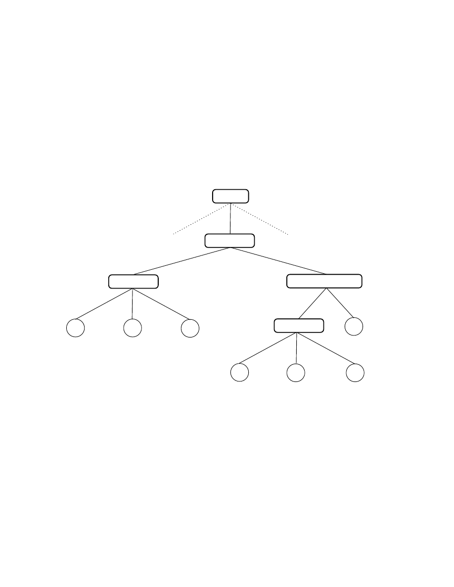
Edge Information

Red

Blue

Green

Incoherent

Coherent

Red

Blue

Green

Edge

Not an edge

Blue

Red

Green

Adjacency

Adjacency

Coherence

Color

Figure 5: An example of histogram refinement.

11

pixels in each bucket based on coherence (i.e.,
generate a CCV). The incoherent pixels can
be refined by tallying the colors of pixels ad-
jacent to the incoherent pixels in a particular
bin. The coherent pixels, in turn, can be fur-
ther refined into those that lie on edges and
those which do not. The coherent pixels on
edges can then be further refined by recording
what colors the coherent regions are adjacent
to. The leaves of the tree, therefore, repre-
sent those images that satisfy these successive
constraints. This set of refinements defines a
compact summary of the image, and remains
an efficient structure to compute and compare.

The best system of constraints to impose

on the image is an open issue. Any combi-
nation of features might give effective results,
and there are many possible features to choose
from. However, it is possible to take advantage
of the temporal structure of a successively re-
fined histogram. One feature might serve as
a filter for another feature, by ensuring that
the second feature is only computed on pixels
which already possess the first feature.

For example, the perimeter-to-area ratio can

be used to classify the relative shapes of color
regions. If we used this ratio as an initial re-
finement on color histograms, incoherent pix-
els would result in statistical outliers, and thus
give questionable results. This feature is bet-
ter employed after the coherent pixels have
been segregated. We call the choice of a sensi-
ble structure of constraints effective feature ex-
traction. Refining a histogram not only makes
finer distinctions between pixels, but functions
as a statistical filter for successive refinements.

Choice of colorspace

Many systems based on color histograms
spend considerable effort on selecting a good
set of colors. Hsu [8], for example, assumes
that the colors in the center of the image are
more important than those at the periphery,

while Smith and Chang [15] use several differ-
ent thresholds to extract colors and regions. A
wide variety of different colorspaces have also
been investigated.

For example, Swain and

Ballard [19] make use of the opponent-axis col-
orspace, while QBIC [4] uses the Munsell col-
orspace.

The choice of colorspace is a particularly sig-

nificant issue for CCV’s, since they use the dis-
cretized color buckets to segment the image. A
perceptually uniform colorspace, such as CIE
Lab, should result in better segmentations and
improve the performance of CCV’s. A related
issue is the color constancy problem [9], which
causes objects of the same color to appear
rather differently depending upon the lighting
conditions. The simplest effect of color con-
stancy is a change in overall image brightness,
which is responsible for the negative exam-
ples obtained in our experiments. Standard
histogramming methods are sensitive to im-
age gain. More sophisticated methods, such
as cumulative histograms [16] or color ratio
histograms [5], might alleviate this problem.

In fact, most proposed improvements to

color histograms can also be applied to CCV’s.
This includes improvements beyond the selec-
tion of better colorspaces. For example, some
authors [17] suggest that color moments be
used in lieu of histograms.

Color moments

could be computed separately for coherent and
incoherent pixels.

CONCLUSIONS

We have described a new method for compar-
ing pairs of images that combines color his-
tograms with spatial information.

Most re-

search in content-based image retrieval has fo-
cused on query by example (where the system
automatically finds images similar to an input
image). However, other types of queries are
also important. For example, it is often useful

12

to search for images in which a subset of an-
other image (e.g. a particular object) appears.
This would be particularly useful for queries
on a database of videos.

One approach to

this problem might be to generalize histogram
back-projection [19] to separate pixels based
on spatial coherence.

It is clear that larger and larger image

databases will demand more complex similar-
ity measures. This added time complexity can
be offset by using efficient, coarse measures
that prune the search space by removing im-
ages which are clearly not the desired answer.
Measures which are less efficient but more ef-
fective can then be applied to the remaining
images. Baker and Nayar [2] have begun to
investigate similar ideas for pattern recogni-
tion problems. To effectively handle large im-
age databases will require a balance between
increasingly fine measures (such as histogram
refinement) and efficient coarse measures.

Acknowledgements

We wish to thank Virginia Ogle for giv-
ing us access to the Chabot imagery, and
Thorsten von Eicken for supplying additional
images. Greg Pass has been supported by Cor-
nell’s Alumni-Sponsored Undergraduate Re-
search Program, and Justin Miller has been
supported by a grant from the GTE Research
Foundation.

References

[1] Farshid Arman, Arding Hsu, and Ming-

Yee Chiu.

Image processing on com-

pressed data for large video databases. In
ACM Multimedia Conference, pages 267–
272, 1993.

[2] Simon Baker and Shree Nayar. Pattern

rejection. In Proceedings of IEEE Con-

ference on Computer Vision and Pattern
Recognition, pages 544–549, 1996.

[3] M. G. Brown, J. T. Foote, G. J. F. Jones,

K. Sparck Jones, and S. J. Young. Au-
tomatic content-based retrieval of broad-
cast news. In ACM Multimedia Confer-
ence, 1995.

[4] M. Flickner et al. Query by image and

video content: The QBIC system. IEEE
Computer, 28(9):23–32, September 1995.

[5] Brian V. Funt and Graham D. Finlayson.

Color constant color indexing.

IEEE

Transactions on Pattern Analysis and
Machine Intelligence, 17(5):522–529, May
1995.

[6] J. Hafner,

H. Sawhney,

W. Equitz,

M. Flickner, and W. Niblack. Efficient
color histogram indexing for quadratic
form distance functions. IEEE Transac-
tions on Pattern Analysis and Machine
Intelligence, 17(7):729–736, July 1995.

[7] Arun Hampapur, Ramesh Jain, and Terry

Weymouth. Production model based dig-
ital video segmentation. Journal of Mul-
timedia Tools and Applications, 1:1–38,
March 1995.

[8] Wynne Hsu, T. S. Chua, and H. K. Pung.

An integrated color-spatial approach to
content-based image retrieval. In ACM
Multimedia Conference, pages 305–313,
1995.

[9] E. H. Land and J. J. McCann. Lightness

and Retinex theory. Journal of the Opti-
cal Society of America, 61(1):1–11, 1971.

[10] Akio Nagasaka and Yuzuru Tanaka. Au-

tomatic video indexing and full-video
search for object appearances.

In 2nd

Working Conference on Visual Database
Systems, October 1991.

13

[11] Virginia Ogle and Michael Stonebraker.

Chabot:

Retrieval from a relational

database of images.

IEEE Computer,

28(9):40–48, September 1995.

[12] K. Otsuji and Y. Tonomura. Projection-

detecting filter for video cut detection.
Multimedia Systems, 1:205–210, 1994.

[13] Alex Pentland, Rosalind Picard, and Stan

Sclaroff. Photobook: Content-based ma-
nipulation of image databases.

Inter-

national Journal of Computer Vision,
18(3):233–254, June 1996.

[14] Rick

Rickman

and

John

Ston-

ham. Content-based image retrieval using
color tuple histograms. SPIE proceedings,
2670:2–7, February 1996.

[15] John Smith and Shih-Fu Chang. Tools

and

techniques

for

color

image

re-

trieval.

SPIE proceedings, 2670:1630–

1639, February 1996.

[16] Thomas M. Strat. Natural Object Recog-

nition. Springer-Verlag, 1992.

[17] Markus Stricker and Alexander Dimai.

Color indexing with weak spatial con-
straints.

SPIE proceedings, 2670:29–40,

February 1996.

[18] Markus Stricker and Michael Swain. The

capacity of color histogram indexing. In
Proceedings of IEEE Conference on Com-
puter Vision and Pattern Recognition,
pages 704–708, 1994.

[19] Michael Swain and Dana Ballard. Color

indexing. International Journal of Com-
puter Vision, 7(1):11–32, 1991.

[20] Patrick Winston and Berthold Horn.

Lisp.

Addison-Wesley, second edition,

1984.

[21] Ramin Zabih, Justin Miller, and Kevin

Mai. A feature-based algorithm for de-
tecting and classifying scene breaks. In
ACM Multimedia Conference, pages 189–
200, November 1995.

[22] HongJiang Zhang, Atreyi Kankanhalli,

and Stephen William Smoliar. Automatic
partitioning of full-motion video. Multi-
media Systems, 1:10–28, 1993.

14