Imaging of Water Flow in Porous Media by Magnetic Resonance Imaging Microscopy

Markus Deurer, Iris Vogeler,* Alexander Khrapitchev, and Dave Scotter

ABSTRACT

pared the column-scale breakthrough of a chloride step-
pulse with a dispersion estimate based on an MRI mea-

Magnetic resonance imaging (MRI) was used to study the flow of

sured slice-scale velocity distribution.

water in a column 14 mm in diameter packed with glass beads. The
sample was fully saturated and water was pumped through the column
using a peristaltic pump, at flow rates of 125 and 250 mL h

⫺

1

. This

THEORY

corresponds to mean velocities of 0.5 and 1 mm s

⫺

1

, given a porosity

of 0.46 m

3

m

⫺

3

. Nuclear magnetic resonance (NMR) images of the

Nuclear Magnetic Resonance

proton density and velocities within a 2-mm slice were taken at a

We will give only some specific background on the theory

spatial resolution of 0.15

⫻ 0.15 ⫻ 2 mm

3

. At a mean pore water

of MRI. A thorough introduction and more details are given

velocity of 1 mm s

⫺

1

we approximated hydrodynamic dispersion using

by Callaghan (1991).

NMR-measured velocity distributions in a 2-mm slice through the
sample. Additionally, we conducted a step pulse tracer experiment

Measurement of Volumetric Water Content

with chloride through the same column and at identical initial and
boundary conditions. We fitted the convection–dispersion equation

The volumetric water content (

␪) at one voxel is directly

to the breakthrough curve and compared the column scale dispersion

proportional to the number of resonating spinning water pro-

of the tracer experiment with the respective NMR estimate derived

tons in the voxel, the so-called spin density,

␳. The precessing

at the slice scale.

macroscopic magnetization at each voxel induces the electric
signal we measure with NMR. This macroscopic magnetization
is caused by the ensemble of precessing microscopic magnetic
moments of the individual resonating spinning water protons,

A

t present it is possible to measure pore characteris-

and is therefore a measure of their density. Consider the spins

tics of porous media three-dimensionally using,

at the spatial position r within the sample occupying an infini-

for example, a series of thin sections (Vogel and Kretz-

tesimal volume dV. The local spin density

␳(r) will contain

schmar, 1996) or computer aided tomography (Perret

␳(r) dV spins. The spatial position of each volume element

et al., 1999). But with these techniques we cannot study

is labeled in three dimensions with magnetic field gradients

which part of all the potential flow pathways are realized

denoted as G

x

, G

y

, G

z

(G ), where the subscripts refer to the

under various initial and boundary conditions. Magnetic

x, y, and z coordinates. They impose on the received signal

resonance imaging (MRI) can be used to obtain infor-

an image position specific frequency ( frequency gradient, e.g.,

mation on soil properties and flow at a high spatial reso-

G

x

) and a phase shift (phase gradient, e.g., G

y

). The signal

lution.

arising from this infinitesimal volume is (Callaghan, 1991):

Magnetic resonance imaging techniques have been

dS(G,t )

⫽ ␳(r)dV exp[iw(r)t]

[1]

used to spatially determine soil water content (Amin et
al., 1994; Hall et al., 1997), and to measure the local

where i denotes the real part of the complex signal and w(r )
is the position specific precession frequency. The latter de-

velocity of water and paramagnetic tracers in porous

pends on the main magnetic field B

0

(applied externally to

media (Seymour and Callaghan, 1997; Sederman et al.,

cause the precession of the water protons) and the gradient

1998) and soils (Pearl et al., 1993; Amin et al., 1994;

G. Therefore, Eq. [1] can be written as (Callaghan, 1991):

Hoffmann et al., 1996; Oswald et al., 1997).

We measured the velocities of moving water protons

dS(G,t )

⫽ ␳(r)dV exp[i(␥B

0

⫹ ␥Gr)t]

[2]

directly with a dynamic imaging pulse sequence (see

where

␥ is the gyromagnetic ratio for

1

H.

Callaghan, 1991). The study aimed to explore the feasi-

For convenience the received signal is mixed with a refer-

bility of measuring the volumetric water content (

␪) and

ence oscillation, canceling out the precession contribution of

velocity in a porous medium at the pore scale. To do

the main magnetic field to the signal. The signal now oscillates

this we studied water flow in a column packed with glass

at

␥Gr. Integrating over the volume of each voxel the signal

beads, 2 mm in diameter. The NMR images of the spin

becomes (Callaghan, 1991):

density (which is directly proportional to

␪) and velocity

S(t )

⫽

冮冮冮

␳(r)exp[i␥Grt]

[3]

distributions were taken within a 2-mm slice through
the column. The voxel size was 0.15

⫻ 0.15 ⫻ 2 mm

3

.

Using the following substitution (the so-called reciprocal space

A second aim was to document the potential of MRI

vector K ):

to analyze the spatial scale dependence of processes
such as hydrodynamic dispersion. To do this we com-

K

⫽

1

2

␲

␥Gt

[4]

M. Deurer, I. Vogeler, and D. Scotter, Environment and Risk Manage-

the received signal S and the spin density

␳ are mutually conju-

ment Group, Hort Research Institute, Private Bag 11-030, Palmerston

gate Fourier pairs (Callaghan, 1991):

North, New Zealand. A. Khrapitchev, Institute of Fundamental Sci-
ences, Massey University, Private Bag 11-222, Palmerston North, New
Zealand. Received 6 June 2001. *Corresponding author (ivogeler@

Abbreviations: CDE, convection–dispersion equation; CLT, convec-

hort.cri.nz).

tive–lognormal transfer; MRI, magnetic resonance imaging; NMR,
nuclear magnetic resonance.

Published in J. Environ. Qual. 31:487–493 (2002).

487

488

J. ENVIRON. QUAL., VOL. 31, MARCH–APRIL 2002

For the lower boundary condition it was assumed that the

S(K)

⫽

冮冮冮

␳(r)exp[i2␲Kr]dr

column was part of an effectively semi-infinite system.

The solution for the flux concentration is given by (Kirkham

␳(r) ⫽

冮冮冮

S(K)exp[

⫺i2␲Kr]dK

[5]

and Powers, 1971, p. 379–420):

Therefore, after Fourier transformation, we can directly

derive the spin density as the spectrum of the Fourier-trans-

C

f

(z,t )

⫽

1
2

冤

erfc.

冢

z

⫺ vt

2

√

Dt

冣

⫹ exp

冢

v z

D

冣

erfc.

冢

z

⫹ vt

2

√

Dt

冣冥

formed signal.

Spatial Measurements of Velocities

[13]

We want to characterize the bulk motion of the spins in

We also predicted the outflow concentration C

f

through

the direction of flow (in our case z ). At the time t

⫽ 0 the

the entire sample using the NMR-measured slice-scale voxel

spins are at position z and move with a longitudinal velocity

velocities. One approach to link measurements of water and/

v

z

. To label and analyze their motion we apply an additional

or solute transport from different scales, in our case the nuclear

(independent of the gradients for spatial encoding) pulsed

MRI measurements in the 2-mm slice and the column scale

gradient g

z

in the direction of flow. For a very short time

␦

tracer experiment, is the use of transfer functions (Jury, 1982;

the spins at z will therefore precess faster. They dephase by

Jury and Roth, 1990). This approach models hydrodynamic

an angle

␾

1

(C.D. Eccles, personal communication, 2000):

dispersion either with a convective–lognormal transfer (CLT)
function (Jury et al., 1987), or with the convection–dispersion

␾

1

⫽ w

1

t

1

⫽ ␥g

z

z

␦

[6]

equation (CDE). In the first case the dispersivity grows lin-

where

␦ is the duration g

z

is applied. After the time

⌬, g

z

is

early with the travel distance and has no asymptotic limit. In

reapplied. Due to the movement along the z axis the protons

the second case it is constant. The CLT is considered to repre-

are now at position z

⫽ v

z

⌬. Consequently, they will rephase

sent the short distance limit and the CDE the long-distance

by an angle

␾

2

:

limit of solute transport (Sposito et al., 1986). Physically, water
and/or solute transport is probably best represented by a tran-

␾

2

⫽ w

2

t

2

⫽ ␥g

z

(z

⫹ v

z

⌬)␦

[7]

sition from a flow in isolated streamtubes (CLT) to one in a

The resultant phase shift is then:

fully interconnected network of flow pathways (CDE). There
are no theoretical concepts to predict the spatial or temporal

␾

2

⫺ ␾

1

⫽ ␥g

z

v

z

⌬␦

[8]

scales for such a transition. Only little experimental evidence

Note that this resulting phase shift is not position-depend-

exists for such a transition (Butters and Jury, 1989).

ent but only velocity-dependent. We repeat this basic experi-

At the observation scale of the 2-mm slice imaged with

ment several times varying either g

z

,

⌬, or ␦. Let us assume

NMR the flow is restricted to isolated areas between the glass

that we vary

⌬. We then obtain a signal amplitude that varies

beads, as they have a diameter of 2 mm. Thus, on this scale

sinusoidally with

⌬ (C.D. Eccles, personal communication,

hydrodynamic dispersion is truly stochastic–convective and

2000):

takes place in isolated stream tubes.

A stochastic–convective transport of water and/or solutes is

S(

⌬) ⫽ S(t ⫽ 0)exp(i[␥g

z

v

z

␦]⌬)

[9]

like a superposition of piston flow processes within individual

where the angular frequency term in the waveform of Eq. [9]

subcolumns (Jury and Roth, 1990). Each voxel within the slice

is proportional to the velocity of the spins.

is hypothesized to be a representative section of one of those

The concept of measuring velocities with MRI (phase shift,

subcolumns. We then use the slice-scale results and the CLT

see Eq. [8]) puts the movement of water in the Lagrangian

to predict the column-scale breakthrough from our NMR mea-

framework (Seymour and Callaghan, 1997). The measured

surements. According to Bear (1972, p. 608–609), at a mean

voxel-scale v

z

is not space-fixed.

flow rate of 1 mm

⫺

1

the effect of diffusion on dispersion is

negligible, as our experiment would be classified to belong to

Solute Transport

his Zone IV, a region of dominant mechanical dispersion.
Hydrodynamic dispersion is then entirely driven by the vari-

We assume that the one-dimensional convection–dispersion

ability of velocities. Knowing the length l of the sample and

equation (CDE) is appropriate for our experimental condi-

the voxel velocities, solutes in each of these subcolumns have

tions: horizontal flow through a homogeneous medium with

a characteristic travel time from the inlet to the outlet, t

l

(s ):

spatially and temporally constant mean longitudinal pore wa-
ter velocities v in the direction of flow (z axis). The CDE is
given by:

t

l

(s)

⫽

l

v

z

(s)

[14]

⳵C

f

⳵t

⫽ D⳵

2

C

f

⳵z

2

⫺ v⳵

C

f

⳵z

[10]

where s denotes the spatial coordinates (x,y ) of the center of
each subcolumn. We assume equal probabilities for solute

where C

f

is the tracer flux concentration and D the longitudinal

molecules to move into each of the subcolumns. The result is

dispersion coefficient. For negligible molecular diffusion D

a probability density function of the travel times of the solute

can be approximated by:

molecules to travel from the inlet to the outlet port, f

f

(l,t ).

The respective flux concentration at the outlet l and at time

D

⫽ ␭v

[11]

t is then given by (Jury and Roth, 1990):

where

␭ is the longitudinal dispersivity.

The column is initially free of chemicals and at time t

⫽ 0

C

f

(l,t )

⫽ C

0

冮

t

0

f

f

(l,t

⬘)dt⬘ ⫽ C

0

P

f

(l,t )

[15]

a tracer with the concentration C

0

is applied as a step pulse

to the inlet end. Thus, the boundary conditions are:

where P

f

(l,t ) is the cumulative travel time distribution func-

C

f

⫽ 0

for z

⫽ 0

and t

⬍ 0

tion. After normalization of C

f

by C

0

, Eq. [15] can be directly

compared with Eq. [13].

C

f

⫽ C

0

for z

⫽ 0

and t

ⱖ 0

[12]

DEURER ET AL.: IMAGING OF WATER FLOW IN POROUS MEDIA BY MRI MICROSCOPY

489

m

3

m

⫺

3

. The inlet and outlet ports occupied only a fraction

METHODS AND MATERIALS

of the proximal and distal surfaces, thereby representing a

Flow Experiments

point-like influx and efflux. These ports were connected to a
silicon tube with a 1.73-mm diameter. For the flow experi-

A column with a 14.1-mm inner diameter and length l of

ments tap water was pumped through the glass beads with a

46 mm was used for the experiment. The column was filled

Pharmacia double syringe pump at rates of 125 and 250 mL

with glass beads 2 mm in diameter giving a porosity of 0.45

h

⫺

1

. This corresponds to mean longitudinal velocities through

the porous medium of v

⫽ 0.5 and 1 mm s

⫺

1

.

For the tracer experiment, a step pulse with C

0

⫽ 0.001 M

KCl was fed directly to the inlet port of the column at a flow
rate of 250 mL h

⫺

1

. The concentrations of chloride were ana-

lyzed with high performance liquid chromatography (HPLC)
(Dionex [Sunnyvale, CA] 500).

Magnetic Resonance Imaging Methods

We used a horizontal wide-bore MRI system. It is based

around an Oxford Instruments 4.7 Tesla superconducting mag-
net and consists of a number of commercial and homebuilt
components (C.D. Eccles, personal communication, 1998).

For the measurement of spin densities we used a two-dimen-

sional spin–echo pulse sequence within a slice of 2 mm. A
field of view of 20

⫻ 20 mm was resolved with 128 phase

steps. The sequence consisted of a 4-

␮s 90⬚ hard pulse and a

180

⬚ soft pulse. We used 10 averages, an echo time of 8.4 ms,

and a repetition time of 1 s.

For the velocity we used a dynamic imaging sequence with

two different parameter sets (“slow” and “fast”). The respec-
tive times

⌬ between the two velocity gradient pulses were

7.9 and 6.5 ms, respectively. For the analysis we combined
the results of both sequences. From the “slow” sequence we
inferred velocities up to 2.4 mm s

⫺

1

and from the “fast” se-

quence velocities that were higher than 2.4 mm s

⫺

1

.

Calibration Measurements

Transformation of Spin Densities into Volumetric
Water Contents

We assumed that the voxels with the highest 5% of spin

densities contain only water. We used the median of this popu-

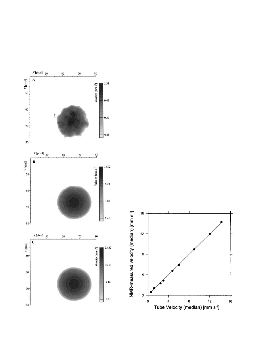
Fig. 1. Spatial distribution of velocities inside a capillary tube with a

Fig. 2. Relationship between the actual applied flow rates and those

diameter of 2.3 mm. The mean velocities were (a ) 0.6, (b ) 6, and
(c ) 14 mm s

⫺

1

.

measured by nuclear magnetic resonance (NMR).

490

J. ENVIRON. QUAL., VOL. 31, MARCH–APRIL 2002

lation for normalization to get the

␪ fractions. For this calcula-

RESULTS

tion we excluded voxels with a zero spin density.

Nuclear Magnetic Resonance Images

of Water Content

Velocity Calibration

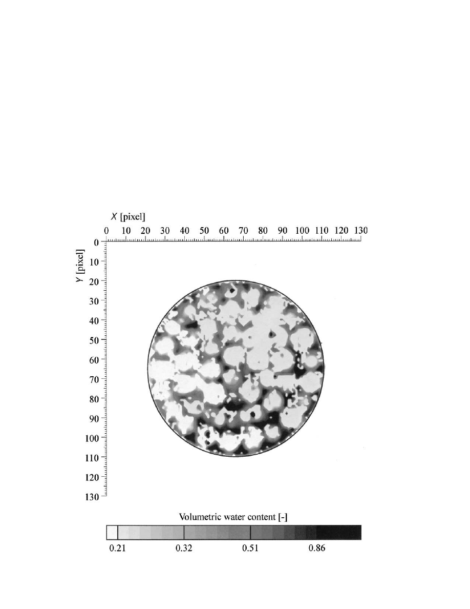
Figure 3 shows an image of the volumetric water

Figure 1 shows the velocity distribution of three of the

content from a 2-mm slice in the column packed with

velocity measurements through the capillary tube, at 9, 90,

glass beads. The regions where the glass beads are and

and 210 mL h

⫺

1

. This corresponds to mean velocities of 0.6,

the regions between them are clearly visible. The mean

6, and 14 mm s

⫺

1

. All three images show a parabolic velocity

value of all these normalized voxels

␪ was 0.44 m

3

m

⫺

3

.

distribution, as expected. At low velocities some distortion

This compares well with the gravimetrically determined

occurs, which is probably due to the shaking of the magnet.
Figure 2 shows the relationship between the actual applied

bulk porosity of 0.45 m

3

m

⫺

3

.

flow rates and those measured by NMR. The relationship is
linear. Different NMR parameter settings had to be used for

Velocity Measurements through Beads of Glass

low (“slow” sequence) and high velocities (“fast” sequence).

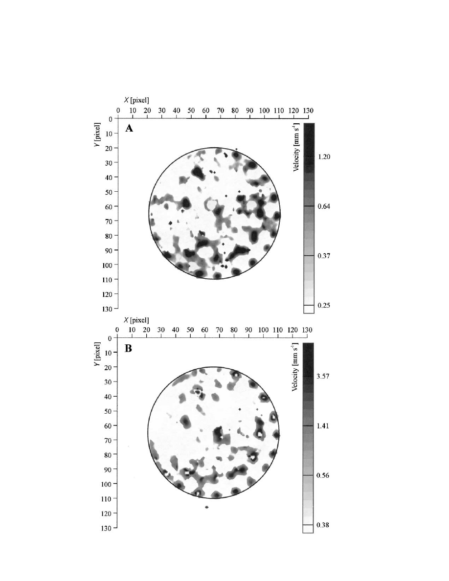
Figure 4 shows the spatial distribution of velocities

These velocity measurements in capillary tubes provided us

between glass beads at the set flow rates of 125 and 250

with a NMR sequence, which we could use to measure velocity
spectra in porous media.

mL h

⫺

1

, corresponding to mean flow rates of 0.5 and

Fig. 3. Nuclear magnetic resonance (NMR) image of the volumetric water content from a 2-mm slice in the center of the column packed with

glass beads.

DEURER ET AL.: IMAGING OF WATER FLOW IN POROUS MEDIA BY MRI MICROSCOPY

491

1 mm s

⫺

1

. For both flow rates two images were taken,

to the wall where the packing is more regular. The mean
velocities calculated from these NMR images agree well

with different settings (according to the calibration mea-
surements). These two images were then overlaid. The

with the actual applied velocities (see Table 1). The
flow rates obtained by multiplying these mean velocities

regions with high velocities are clustered and occur close

Fig. 4. Spatial distribution of velocities in the glass bead mean flow rates of (a ) 0.5 and (b ) 1 mm s

⫺

1

.

492

J. ENVIRON. QUAL., VOL. 31, MARCH–APRIL 2002

Table 1. Comparison between applied flow rates (Q ) and veloci-

ties (v ) and those obtained by nuclear magnetic resonance
(NMR).

Q

v

mL h

⫺

1

mm s

⫺

1

Applied

125

250

0.5

1

NMR, bulk characteristics

137

249

0.55

1

NMR, voxel-based

66

115

with the NMR measured

␪, also agree well with the

actual ones (see Table 1, bulk characteristics). However,
when the voxel-based velocities were multiplied by the
voxel-based

␪, the flow rates obtained were only about

50% of those applied. We think this discrepancy be-
tween flux based on voxels and flux measured is mainly
due to errors in the spin density measurements. The
glass beads themselves impose small local magnetic
fields. Therefore, in the vicinity of the surface of the
glass beads the magnetic susceptibility of water changes.
This inhomogeneity of the magnetic susceptibility leads
to an additional transverse relaxation and consequential
signal attenuation (Callaghan, 1990). This effect is used
to analyze, for example, the pore size distributions of

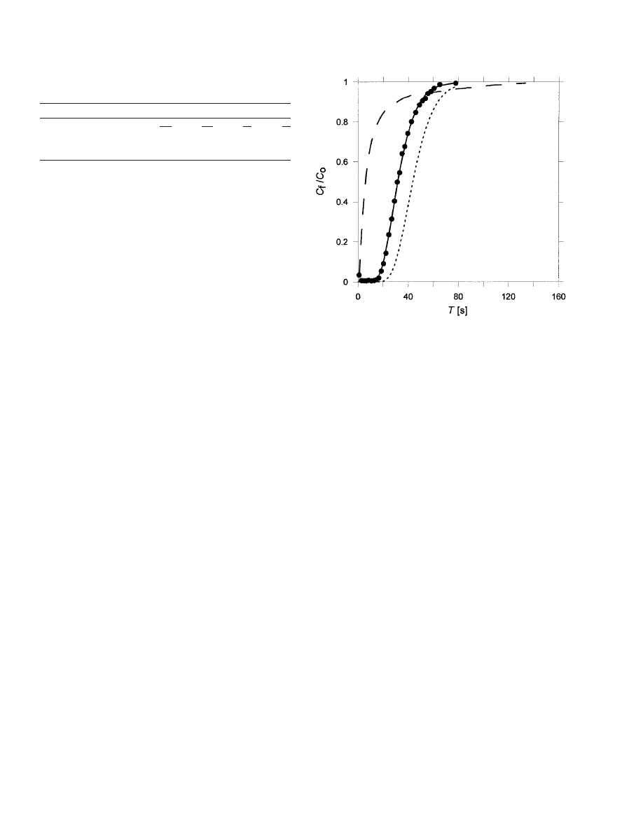
Fig. 5. Measured and predicted breakthrough curve (BTC) of chlo-

ride using the convection–dispersion equation (CDE) with theoret-

porous materials (Davies et al., 1991; Allen et al., 1998).

ical parameter values (dotted line), and with fitted parameter values

In the study of Hall et al. (1997) using a standard spin–

(solid line). Also shown is the prediction based on the velocity

echo sequence, only 0.2 to 57% of the bulk water was

distribution measured by nuclear magnetic resonance (NMR) (bro-

detected for soils of varying types including sands. Cur-

ken line).

rently, we try to use different NMR protocols such as
an inversion–recovery sequence (Callaghan, 1991) to

column scale was about the bead diameter (Pfannkuch,

overcome this problem. For the calibration we omitted

1963). But all of them used a uniform Neumann-type

voxel values that had zero spin density. These are voxels

boundary condition (Neumann et al., 1974). In many

with very low water contents. Voxels with small water

situations we can encounter a similar boundary condi-

contents contain either small pore(s) or mainly glass

tion rather than a homogeneous entry of water and/

bead material. The effects of a changing magnetic sus-

or solutes into the soil (e.g., drip irrigation systems,

ceptibility are strongest close to the surface of the glass

preferential or unstable flow). This shows the depen-

beads. Therefore, voxels with small water contents are

dence of transport parameter values on the type of

likely to show the resulting effect of signal attenuation

boundary condition.

most pronounced. In those voxels the underestimation

Using only the voxel-based slice-scale velocities for

of the spin density, and thus the water content, would

an estimate of the normalized outflow concentration

be highest. If the respective voxel velocities are simulta-

(see broken line in Fig. 5), the breakthrough starts much

neously high then their contribution to the overall flux

earlier and shows pronounced tailing. The dispersivity

will be considerable. But generally, all voxels and their

from this curve is estimated as 63 mm and the respective

water contents that are influenced by the inhomogeneity

fractional transport volume as only 0.129. The extrapo-

of magnetic susceptibility due to the glass bead material

lation of the slice measurement neglects the formation

are affected.

of a network of flow paths. This is indirect microscopic
experimental proof for a scale-dependent transition

Tracer Experiment

from a stochastic–convective to a convective–dispersive

The breakthrough curve (BTC) of chloride is shown

transport process. The variability of the velocity distri-

in Fig. 5. Also shown as the dotted line is the prediction

bution itself is obviously scale dependent and a result of

of the convection–dispersion equation (CDE) using a

the flow network configuration. Our findings emphasize

dispersivity (

␭) of 2 mm (theoretical value according

that we need more research in this particular area con-

the diameter of the glass beads; Dullien, 1992), and

cerning the scales of the transition from a stochastic–

assuming that all the water is mobile (

␪

m

). However,

convective to a convective–dispersive dispersion regime.

the chloride appears in the leachate much earlier than

We think that NMR has the potential to solve these

predicted. Next, the CDE was fitted to the data, giving

questions in the future. It also shows that what we inter-

a

␭ of 3 mm and a ␪

m

of 0.33 (solid line). The dispersivity

pret as the mobile (transport volume) water fraction

as a correlation length of the pore space is larger than

might be rather a function of the flow network, the

the glass-bead diameter, and the respective transport

observation scale, and the type of boundary condition.

volume is smaller than the porosity. This might be due
to our experimental setup, with a point-source entry of

OUTLOOK

water and/or solutes as an upper boundary condition.
Existing macroscopic experiments measuring dispersion

In a few experiments NMR has been used to study

the transport of water and/or solutes in soils (Pearl et

in glass bead porous media show that dispersivity on the

DEURER ET AL.: IMAGING OF WATER FLOW IN POROUS MEDIA BY MRI MICROSCOPY

493

ards, and B.W. Bache. 1994. Magnetic resonance imaging of soil-

al., 1993; Hoffman et al., 1996; Amin et al., 1997; Hem-

water phenomena. Magn. Reson. Imag. 12:319–321.

minga and Buurman, 1997; Cislerova´ et al., 1999).

Bear, J. 1972. Dynamics of fluids in porous media. Elsevier, New York.

Natural soils regularly contain ferromagnetic or para-

Butters, G.L., and W.A. Jury. 1989. Field scale solute transport of

magnetic elements, for example, free iron oxides or

bromide in an unsaturated soil. 2. Dispersion modeling. Water
Resour. Res. 25:1583–1589.

copper sulfates, respectively. These lead to faster spin–

Callaghan, P.T. 1990. Susceptibility-limited resolution in nuclear mag-

spin and spin–lattice relaxation times. Consequently,

netic resonance microscopy. J. Magn. Reson. 87:304–318.

when the signal is measured a considerable part of it has

Callaghan, P.T. 1991. Principles of nuclear magnetic resonance micros-

already been attenuated and the results are accordingly

copy. Clarendon Press, Oxford.

biased. The study of Greiner et al. (1997) took advan-

Cislerova´, M., J. Votrubova´, T. Vogel, M.H.G. Amin, and L.D. Hall.

1999. Magnetic resonance imaging and preferential flow in soils.

tage of this effect using copper sulfate as a paramagnetic

p. 397–411. In Proc. of the Int. Workshop Characterization and

tracer. Other soil physical and chemical properties, such

Measurement of the Hydraulic Properties of Unsaturated Porous

as high clay contents (which result in pronounced inho-

Media, Riverside, CA. 22–24 Oct. 1999. Part I. USDA, River-

mogeneities in the magnetic susceptibility), organic mat-

side, CA.

ter, and even exchangeable cations such as calcium and

Davies, S., K.J. Packer, D.R. Roberts, and F.O. Zelanya. 1991. Pore

size distributions from NMR spin–lattice relaxation data. Water

potassium can also reduce the relaxation times (Hall et

Resour. Res. 9:681–685.

al., 1997). However, advances in NMR technology and

Dullien, F.A.L. 1992. Porous media. Fluid transport and pore struc-

the development of new adapted pulse sequences might

ture. 2nd ed. Academic Press, San Diego, CA.

solve these problems.

Greiner, A., W. Schreiber, G. Brix, and W. Kinzelbach. 1997. Magnetic

resonance imaging of paramagnetic tracers in porous media: Quan-
tification of flow and transport parameters. Water Resour. Res.

CONCLUSIONS

33:1461–1473.

Hall, L.D., M.H.G. Amin, E. Dougherty, M. Sanda, J. Votrubova,

The study has described the use of NMR to observe

K.S. Richards, R.J. Chorley, and M. Cislerova. 1997. MR properties

water movement in porous media, here in columns

of water in saturated soils and resulting loss of MRI signal in water

packed with glass beads. The volumetric water content

content detection at 2 Tesla. Geoderma 80:431–448.

inferred from the NMR image agreed well with the one

Hemminga, M.A., and P. Buurman. 1997. NMR in soil science. Ge-

oderma 80:221–224.

determined gravimetrically. The mean velocities and

Hoffmann, F., D. Ronen, and Z. Pearl. 1996. Evaluation of flow

flow rates obtained by NMR also agreed well with the

characteristics of a sand column using magnetic resonance imaging.

applied flow rate when based on bulk characteristics.

J. Contam. Hydrol. 22:95–107.

However, when the flow rate was calculated on a voxel

Jury, W.A. 1982. Simulation of solute transport using a transfer func-

tion model. Water Resour. Res. 18:363–368.

basis only about 50% of the actual applied flow rate

Jury, W.A., D.D. Focht, and W.J. Farmer. 1987. Evaluation of pesti-

was obtained. This was probably due to a spin density

cide ground water pollution potential from standard indices of

distribution that was biased toward voxels with small

soil–chemical adsorption and biodegradation. J. Environ. Qual. 16:

volumetric water contents: spin–spin relaxation times

422–428.

will be rapid and due to technical limitations no signal

Jury, W.A., and K. Roth. 1990. Transfer functions and solute move-

ment through soil. Theory and application. Birkha¨user Verlag,

can be detected. We intend to further improve our NMR

Basel, Switzerland.

measuring technique.

Kirkham, D., and W.L. Powers. 1971. Advanced soil physics. Wiley

We compared the results of a conventional break-

Interscience, New York.

through experiment (column-scale) with the prediction

Neumann, S.P., R.A. Feddes, and E. Bresler. 1974. Finite element

based on the slice-scale velocity distribution obtained

simulation of flow in saturated–unsaturated soils considering water
uptake by plants. 3rd Annu. Rep., Project A10-SWC-77. Hydraulic

by MRI. We showed that solute transport parameters

Engineering Lab., Technion, Haifa, Israel.

such as the dispersivity and the transport volume depend

Oswald, S., W. Kinzelbach, A. Greiner, and G. Brix. 1997. Observing

on the network of flow pathways, the type of boundary

of flow and transport processes in artificial porous media via mag-

condition, and the observation scale. Thus, MRI can

netic resonance imaging in three dimensions. Geoderma 80:417–
429.

give valuable information concerning transport pro-

Pearl, Z., M. Magaritz, and P. Bendel. 1993. Nuclear magnetic reso-

cesses in porous media, which at present can only be

nance imaging of miscible fingering in porous media. Transp. Po-

studied on a macroscopic scale.

rous Media 12:107–123.

Perret, J., S.O. Prasher, A. Kartzas, and C. Langford. 1999. Three-

ACKNOWLEDGMENTS

dimensional quantification of macropore networks in undisturbed
soil cores. Soil Sci. Soc. Am. J. 63:1530–1543.

The study was funded by the Royal Society through a Mars-

Pfannkuch, O. 1963. Contribution a l’etude des deplacements de flu-

den Fund, Contract HRT 805. We would like to thank Paul

ides miscible dans un milieu poreux. Revue de l’Institute Francais

Callaghan and Sarah Codd for many helpful discussions and

du Petrole 18:215–270.

Sederman, A.J., M.L. Johns, P. Alexander, and L.F. Gladden. 1998.

Brent Clothier for the encouragement to do this work.

Visualization of structure and flow in packed beads. Magn. Reson.
Imag. 16:497–500.

REFERENCES

Seymour, J.D., and P.T. Callaghan. 1997. Generalized approach to

NMR analysis of flow and dispersion in porous media. AICHE J.

Allen, S., M. Mallet, M.E. Smith, and J.H. Strange. 1998. Susceptibility

43:2096–2111.

effects in unsaturated porous silica. Magn. Reson. Imag. 16:597–

Sposito, G., W.A. Jury, and V. Gupta. 1986. Fundamental problems

600.

in the stochastic convection–dispersion model of solute transport

Amin, M.H.G., R.J. Chorley, K.S. Richards, L.D. Hall, T.A. Carpen-

in aquifers and field soils. Water Resour. Res. 22:77–88.

ter, M. Cislerova´, and T. Vogel. 1997. Study of infiltration into

Vogel, H.J., and A. Kretzschmar. 1996. Topological characterization

a heterogeneous soil using magnetic resonance imaging. Hydrol.

of pore space in soil-sample preparation and digital image-pro-

Processes 11:471–483.

cessing. Geoderma 73:23–38.

Amin, M.H.G., L.D. Hall, R.J. Chorley, T.A. Carpenter, K.S. Rich-