
Introduction to Computer Algorithms
Lecture Notes
(undergraduate CS470 course)
taught by
Grzegorz Malewicz
using the text
Cormen, Leiserson, Rivest, Stein: Introduction to Algorithms (2nd Edition). MIT Press (2001)
supplemented by
Kleinberg, Tardos: Algorithm Design. Addison-Wesley (2005)
and
Knuth: The Art of Computer Programming. Addison-Wesley
at the Computer Science Department
University of Alabama
in 2004 and 2005
Copyright Grzegorz Malewicz (2005)

2
Contents
1
INTRODUCTION 3
1.1
The stable matching problem
3
1.2
Notion of an algorithm
9
1.3
Proving correctness of algorithms
10
1.4
Insertion sort
12
1.5
Analysis of running time
15
1.6
Asymptotic notation
17
2
SORTING 19
2.1
Mergesort
19
2.1.1
Recurrences
24
2.2
Quicksort
33
2.3
Randomized quicksort
37
2.4
Lower bound on the time of sorting
43
2.5
Countingsort
46
2.6
Radixsort
47
3
DYNAMIC PROGRAMMING
49
3.1
Assembly-line scheduling
50
3.2
Matrix chain multiplication
54
3.3
Longest common substring
59
4
GRAPH ALGORITHMS
63
4.1
Breadth-first search
64
4.2
Depth-first search
70
4.3
Topological sort
75
4.4
Minimum Spanning Tree
78
4.4.1
Prim’s algorithm
82
4.5
Network Flow
83
4.5.1
Ford-Fulkerson Algorithm
84
4.6
Maximum matchings in bipartite graphs
94
4.7
Shortest Paths
97
4.7.1
Dijkstra’s algorithm
97
4.7.2
Directed acyclic graphs with possibly negative edge lengths
100
4.7.3
Bellman-Ford
104

3
1 Introduction
1.1 The stable matching problem
Today we will look at the process of solving a real life problem by means of an algorithm.
Motivation
Informal setting: males and females that want to find partners of opposite gender.
• we have a certain number of males and females
• each male interacts with females and forms preferences
• each female interacts with males and forms preferences
Say males propose, and females accept or decline. Finally we somehow arrive at a way to match males
with females.
What could destabilize in this process?
retracting acceptance (and “domino effect”): Alice prefers Bob to Mike, but Bob cannot make up his
mind for a long time. Meanwhile Mike has proposed to Alice. Alice have not heard from Bob for a long
time, so she decided to accept Mike. But later Bob decided to propose to Alice. So Alice is tempted to
retract acceptance of Mike, and accept Bob instead. Mike is now left without any match, so he proposes to
some other female, which may change her decision, and so on --- domino.
retracting proposal (and “domino effect”): now imagine that Bob initially proposed to Rebecca, but he
later found out that Kate is available, and since he actually prefers Kate to Rebecca, he may retract his
proposal and propose to Kate instead. If now Kate likes Bob most, she may accept the proposal, and so
Rebecca is left alone by Bob.
We can have a lot of chaos due the switching that may cause other people to switch. Is there some way to
match up the people in a “stable way“?
[[this is a key moment in algorithm design: we typically begin with some vague wishes about a real world
problem, and want to do something “good” to satisfy these wishes, and so the first obstacle to overcome
is to make the wishes less vague and determine what “good” means; we will now start making the
objectives more concrete]]
What could stabilize this process?
We have seen how a match can be bad. How can we get a stable match? Say that Bob is matched with
Alice. If Kate comes along but Bob does not like her so much, then Bob has no incentive to switch.
Similarly, if Mike comes along but Alice does not like him as much as she likes Bob, then Alice has no
incentive to switch, either.
So a matching of males with females will be stable, when for any male M and female F that are not
matched, they have no incentive to get matched up, that is:
a) M prefers his current match over F (so M has no incentive to retract his proposal), or
b) F prefers her current match over M (so F has no incentive to retract her acceptance).
If, however both M likes F more, and F likes M more than their current matches, then M and F would
match up [[leading possibly to chaos, since now the left-alone used-to-be matches of M and F will be
looking for partners]].
4
So we have motivated the problem and began formalizing it.
Problem statement
We introduce some notation that will be helpful in describing the problem. [[we already informally used
some of the subsequent notation]] Let M={m
1
,…,m
n
} be the set of males and F={f
1
,…,f
r
} be the set of
females [[here the number n of males does not have to be equal to the number r of females]]. A matching
S is a subset of the Cartesian product M
×F [[think of S as a set of pairs of males and females]] with the
property that every male is in at most one pair and every female is also in at most one pair [[matching is
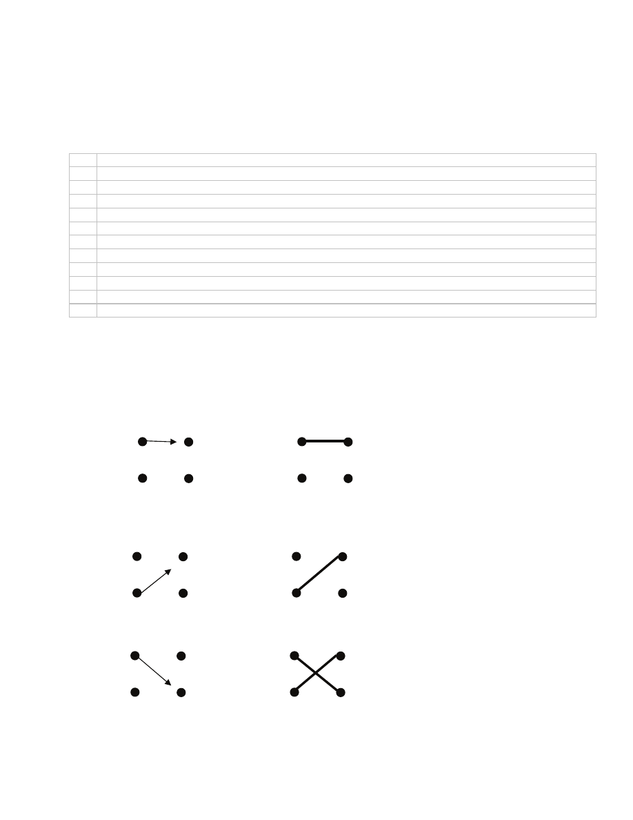
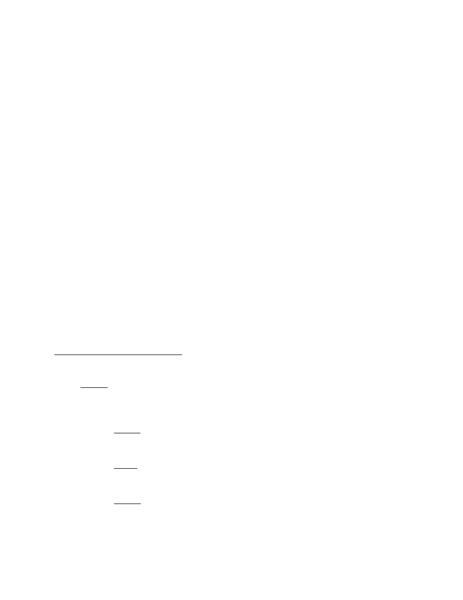
basically a way to formalize the notion of allowed way to pair up males and females]]. Example [[a
segment represents a pair in S]]:
Suppose that we want to match every male to exactly one female, and vice versa [[this is a restriction on
our original problem; we impose it for simplicity---in general, as we are formalizing a problem, we may
decide to make some simplifying assumptions]]. A perfect matching is a matching S where every male
and every female occurs in exactly one pair [[just “every female” is not enough, because n may be not
equal to r---see above]].
Obviously, when n
≠r we cannot match ever male with exactly one female and every female with exactly
one male. [[how many different perfect matching are there, when there are n males? n factorial]]
How do we formalize the notion of the “preference”? [[here the class should propose some ways]] Let us
say that each male ranks every female, from the highest ranked female that he likes the most to the lowest
ranked female that he likes the least. So for each male we have a ranking list that we call preference list.
Similarly, each female has a preference list. [[in practice we may have partial lists, when say a female has
not decided about the attractiveness of a male, or we may have ties when two or more males have the
same attractiveness as seen by a female --- we do not allow this here, again we simplify the problem]]
We want to define a notion of a “stable” perfect matching. Let us then recall what could cause a perfect
matching to be “unstable”. What would make an unmatched pair to want to match up? [[this links to what
we already said, so the reader should be able to define it]] Say that a pair (m,f) is not in S. Male m and
female f are matched to some other partners [[because S is a perfect matching]]. If m prefers f more than
he prefers his current partner, and f prefers m more than she prefers her current partner, then m and f
would have incentive to match up! We then say that the pair (m,f) is an instability with respect to S. A
matching S is stable, if S is a perfect matching and there are no instabilities with respect to S.
m
3
m
2
m
1
f
2
f
1
matching S={(m
1
,f
2
)}
m
3
m
2
m
1
f
2
f
1
not a matching S={(m
1
,f
2
),(m
3
,f
2
)}
m
2
m
1
f
2
f
1
perfect matching
S={(m
1
,f
2
), (m
2
,f
1
)}
5
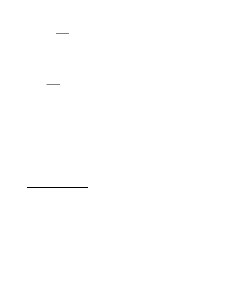
Example 1: unique stable matching, both males and females are perfectly happy [[each matched up with
its highest preference partner]]
Example 2: two stable matchings, either both males are perfectly happy (but not females) or both females
are perfectly happy (but not males) [[for instability to exists, both must prefer each other over current
partners, one preference is not enough!]]
We can now formally state our goal: given n males and n females and their preference lists, we want to
find a stable matching S, if one exists, or state “there is no such matching”, if no stable matching exists.
[[notice how we “transformed” an intuitive wish or vague problem statement into a formal problem
statement --- i.e., it is clear what a possible solution is --- naively, we could consider all n! perfect
matchings S, and for each such S we consider every pair (m,f) not in S to see if the pair is an instability
with respect to S]]
The main goal now is to answer two questions:
1) Does there always exist a stable matching?
2) If so, how can we compute it quickly?
Algorithm
[[we will propose an approach that seems to be reasonable i.e., we guess the algorithm]]
Here is an algorithm that we propose. Initially everybody is unmatched. We will be trying to match
people up based on their preferences. During the process, some males may get matched up with females,
but may later get freed when competitors “win” the female. Specifically, we pick a male m that is
unmatched and has not yet proposed to every female. That male proposes to the highest ranked female f
to whom the male has not yet proposed. The female f may or may not be already matched. If she is not
m
2
m
1
f
2
f
1
preference lists
m
1
: f
2
, f
1
m
2
: f
1
,f
2
f
1
: m
1
, m
2
f
2
: m
2
, m
1
m
2
m
1
f
2
f
1
in (m
1
,f
1
)
m
1
does not
prefer to match-up
in (m
2
,f
2
)
m
2
does not
prefer to match-up
in (m
1
,f
2
)
f
2
does not
prefer to match-up
in (m
2
,f
1
)
f
1
does not
prefer to match-up
m
2
m
1
f
2
f
1
preference lists
m
1
: f
2
, f
1
m
2
: f
1
,f
2
f
1
: m
2
, m
1
f
2
: m
1
, m
2
in (m
1
,f
1
)
neither m
1
nor
f
1
prefers to match-up
in (m
2
,f
2
)
neither m
2
nor
f
2
prefers to match-up
6
matched, then (m,f) get matched-up. It could, however, be that f is already matched to a male m’. Then if
the female prefers m, she gives up m’, and gets matched up with m, thus leaving m’ free. If the female
still prefers m’, then m remains free (m has no luck with f).
Here is a pseudocode for the algorithm
1 let every male in M={m
1
,...,m
n
} and every female in F={f
1
,...,f
n
} be free
2 while there is a free male m who has not yet proposed to every female
3 let f be the highest ranked female to whom m has not yet proposed
4 if f is free, then
5 match m with f (m and f stop being free)
6 else
7 let m’ be the male currently matched with f
8 if f ranks m higher than m’, then
9 match f with m, and make m’ free
10 else
11 m remains free
12 return the matched pairs
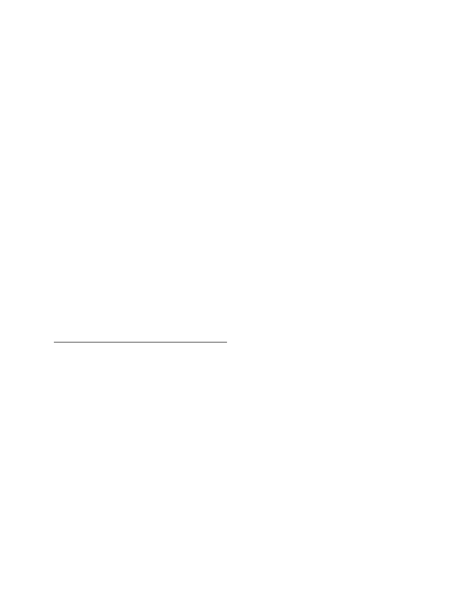
Example
Preference lists
m
1
: f
1
, f
2
m
2
: f
1
, f
2
f
1
: m
2
,m
1
f
2
: m
2
,m
1
First
Then
Then
m
1
m
2
f
1
f
2
propose
m
1
m
2
f
1
f
2
accept
m
1
m
2
f
1
f
2
propose
m
1
m
2
f
1
f
2
switch
m
1
m
2
f
1
f
2
propose
m
1
m
2
f
1
f
2
accept

7
It may be unclear that the algorithm returns a stable matching, let alone a perfect matching [[how do we
even know that every male gets matched to a unique female?]]
Algorithm analysis
We will show that the algorithm is correct, that is that it runs for a finite number of steps, and when the
algorithm halts the set of matched up pairs forms a stable matching.
Fact 1 [[Female view]]
Any female f is initially free. Once she gets matched up, she remains matched up (if changes partners,
always for a better male in terms of her preference list)
Fact 2 [[Male view]]
Any male m is initially free. The male may become matched, then free, then matched again, and so on
(always to a worse female in terms of his preference list)
Theorem
The algorithm performs no more than n
2
iterations of the while loop.
Proof
[[[here class brainstorms ideas]] The key idea is to come up with a quantity that keeps on growing with
each iteration, such that we know that this quantity cannot grow beyond a certain bound.
Recall that the while loop iterates as long as there is a free male that has not proposed to every female.
Then such male proposes to that female. So the number of proposals increases by one at every iteration.
What is the largest number of proposals? Notice that once a male proposes, he never again proposes to the
same female. So each male can propose at most n times, and so the total number of proposals is at most
n
2
, as desired.
█
Thus the algorithm clearly terminates. What remains to be seen is whether the set of pairs returned by the
algorithm is a perfect matching, and then if the matching is stable.
First we show a weaker condition --- pairs form a matching.
Lemma 1
At the end of every iteration, the pairs matched up constitute a matching.
Proof
[[Loop invariant technique]] We will show that if pairs form a matching at the beginning of any iteration
[[at most; at most]], then they also form a matching at the end of the iteration. This will be enough,
because at the beginning of the first iteration the set of matched pairs is empty, and so clearly is a
matching.
Pick any iteration, and let S
beg
be the set of pairs matched up at the beginning of the iteration, and S
end
at
the end. Suppose that S
beg
is a matching. What could happen throughout the iteration? We inspect the
code. Note that m is free. If f is free, too, then m gets matched up with f in line 5, and so S
end
is also a
matching. If, however, f is not free, then f is matched with m’ and to no one else since S
beg
is a matching,
and we either substitute m for m’ or not, so again S
end
is a matching.
█

8
Lemma 2
Consider the end of any iteration. If there is an unmatched male at that time, then there is an unmatched
female.
Proof
Let m be an unmatched male. We reason by contradiction. Suppose that every female is matched. By
Lemma 1 we know that the set of matched pairs forms a matching. But then every male is matched to at
most one female [[by the definition of matching]], while there are n matched females, so there must be at
least n matched males. Recall that m is unmatched, so there are at least n+1 males, a contradiction since
we know that there are exactly n males.
█
Proposition
The set of matched up pairs returned by the algorithm forms a perfect matching.
Proof
Suppose that the while loop exits with a set of matched pairs that is not a perfect matching. We know that
at the end of every iteration the set is a matching, by Lemma 1. Hence we only need to check if every
male is matched to exactly one female [[from that it will follow that every female is matched to exactly
one male, because the number of males is equal to the number of females]]. Suppose that there is an
unmatched male m. Then by Lemma 2, there is an unmatched female f. But this means that no one has
ever proposed to the female (by Fact 2, since otherwise the female will remain matched). In particular m
has not proposed to f. But the then the while loop would not exit, a contradiction.
█
So we are almost done, except that we need to show that the matching is stable.
Theorem
The set of pairs returned by the algorithm is a stable matching.
Proof
Since the set is a perfect matching by the Proposition, we only need to show that there are no instabilities.
Assume, by way of contradiction, that there is an instability (m,f) in the set. This means that m in matched
to some other female f’ whom he prefers less, and f is matched to other male m’ whom she prefers less.
pairs
( m , f’ )
( m’ , f )
preferences
m: ... f ... f’ ...
f: ... m ... m’ ...
Female f’ must be the last female to whom m proposes [[since (m,f’) is in the set when the algorithm
exits]]. But f is higher on his preference list, so he must have proposed to f earlier, and must have been
declined by f. So at the time of declining, f must have been matched with a male m’’ whom f prefers more
than m.
f: ... m’’ ... m
Recall that a female can change her match only to someone she prefers more [[by Fact 2]], so she must
prefer m’ even more than m’’
f: ... m’ ... m’’ ... m

9
But we know that f prefers m more than m’, while we conclude that the opposite must be true. This is a
desired contradiction.
█
1.2 Notion of an algorithm
Algorithm is a description of how to transform a value, called input, to a value, called output. The
description must be precise so that it is clear how to perform the transformation. The description can be
expressed in English, or some other language that we can understand, such as C++. An algorithm may not
halt, or may halt but without transforming the input to an output value.
A computational problem is a specification of input-output relation.
Example sorting problem
Input: A sequence of n
≥
1 numbers <a
1
,a
2
,…,a
n
>
Output: A permutation (reordering) <a’
1
,a’
2
,…,a’
n
> of the input sequence such that a’
1
≤ a’
2
≤ …≤ a’
n
.
For example, given <2,1,5,3,3> as an input, we desire to transform it into <1,2,3,3,5> [[showing
duplicates should help clarify]]. The input sequence is called instance of the sorting problem.
Algorithm can be used to solve a computational problem. An algorithm for a computational problem is
correct if it transforms any input specified by the problem into an output specified by the problem for this
input [[as given by the input-output relation]]. Such correct algorithm is said to solve the computational
problem. An incorrect algorithm may not halt on some inputs or may transform some inputs into wrong
outputs [[such incorrect algorithms may still be useful, for example when they work well on an
overwhelming fraction of inputs and they are very fast for such inputs; Monte Carlo and Las Vegas]]
There are many computational problems that can be solved by algorithms
• finding information on the web -- Google uses links leading from a page to other pages to decide
which pages are more important [[PageRank]]
• encrypting information to enable electronic commerce -- the famous RSA algorithm requires finding
large primes
• finding short routes from one city to other city -- the Dijkstra’s algorithm for finding shortest paths in
a graph
• assigning crew members to airplanes -- airlines want to use few crew members to run the planes,
while there are governmental restrictions on how crew members can be assigned [[problem is called
crew rostering]]
So there is a wealth of interesting computational problem that occur in practice which one would like to
solve. This motivates the study of algorithms.
There may be several algorithms that solve a given computational problem. Which one is best? How do
we determine what best means?
Efficiency of an algorithm is typically its speed -- so faster algorithm would be more efficient than slower
algorithm. There are other measures [[memory usage, complexity of writing and maintaining code]]. If
computers were infinitely fast and memory was free, we would not care for how quickly an algorithm runs
and how much memory it consumes. However, we would still like to know if an algorithm for a problem
is correct [[does it produce a desired output given any desired input?]].

10
There are some problems for which no quick algorithm has ever been found [[a precise meaning of
“quick” will be given later in the course]]. Some of this problems form a class called NP-complete
problems. The class has the property that if you find a quick algorithm for one problem from the class,
you can design a quick algorithm for any other problem from this class. One such problem is to find a
shortest path that visits each city exactly once and comes back the starting city [[called Traveling
Salesman Problem]]. It is remarkable that nobody has ever found any quick algorithm for any NP-
complete problem. People believe that there is no quick algorithm for any NP-complete problem. So do
not be surprised if you cannot find a quick algorithm for a computational problem. We will study this
fascinating area of algorithms towards the end of the course.
The goal of this course is to teach you several techniques for designing algorithms and analyzing
efficiency of algorithms, so you should be able to design an efficient algorithm that solves a computational
problem that you encounter [[we need to be modest -- some problems are so hard that we may not be able
to solve them, but we should be able to solve some easier problems]].
1.3 Proving correctness of algorithms
When trying to prove that an algorithm solves a problem, we may encounter a problem: algorithm may
have a loop that may run for arbitrarily long. How can we write a “short” proof of correctness when the
execution can be arbitrarily long? We will use the following idea. We will try to find a property that is
always true no matter how many times the loop iterates, so that when the loop finally terminates, the
property will imply that the algorithm accomplished what it was supposed to accomplish.
We illustrate the idea on a simple problem of searching through a table. Suppose that we are given a table
A and a value v as an input, and we would like to find v inside the table, if v exists in the table.
Specifically, we must return NIL when no element of the table is equal to v, and when one is equal to v,
then we must return i so that A[i]=v. We call this the searching problem.
Algorithm
Search(A,v)
1
► length[A]≥1
2 i
← NIL
3
if A[1]=v then
4
i ← 1
5 j
← 1
6
while j < length[A] do
7
j ← j+1
8
if A[j]=v then
9
i ← j
10 return
i
The algorithm scans through the table from left to right, searching for v. We formulate a property that we
believe that is true as we iterate.
Invariant:
(if A[1…j] does not contain v, then i=NIL) and
(if A[1…j] contains v, then A[i]=v) and
(j
∈{1,…,length[A])

11
Initialization:
Line 2 checks if A[1] contains v, and if so line 3 sets i to 1, if not i remains NIL. Then j gets assigned 1.
Note that the length of A is at least 1, so such j is in {1,…,length[A]}. So the invariant is true right before
entering the while loop.
Maintenance:
We assume that the invariant is true right before executing line 7. Since line 7 is executed, loop guard
ensures that j<length[A], and invariant ensures that {1,…,length[A]}. Hence after j has been incremented
in line 7, j is still in {1,…,length[A]}. Let j have the value right after line 7 has been executed. We
consider two cases:
Case 1: If A[1…j] does not contain v, then A[1…j-1] does not contain v either, and so by invariant i was
NIL right before executing line 7, and condition in line 8 will evaluate to false, so i will remain NIL after
the body of the while loop has been executed. So invariant is true at the end of the body of the while loop.
Case 2: If A[1…j] contains v, then either A[1…j-1] contains v or A[j] contains v. If A[j]=v, then the
condition in line 8 will evaluate to true, and i will be set to j in line 9. So A[i]=v at the end of the body of
the while loop. However, if A[j] is not v, then by our assumption of case 2, it must be the case that
A[1…j-1] contains v, and so by invariant A[i]=v right before executing line 7. But lines 7 does not
change i, and line 9 does not get executed. So in this case the invariant holds at the end of the body of the
while loop.
Termination:
When the loop terminates, j
≥length[A] and the invariant holds. So j=length[A]. Then the first two
statements of the invariant imply the desired property about i.
So far we have shown that if the algorithm halts, then the algorithm produces the desired answer.
Finally, we must show that the algorithm always halts. Observe that j gets incremented by one during
every iteration, and so the algorithm eventually halts.
Hence the algorithm solves the searching problem.
The method of proving correctness of algorithms is called loop invariant. Here is an abstract
interpretation of the method.
Initialization
Inv=true
If the body of the loop never executes
If the body of the loop executes at least once,
but a finite number of times
first iteration
so Inv=true
Maintenance
Inv=true at the beginning => Inv=true at the
end
so Inv=true

12
so Inv=true
second iteration
so Inv=true
Maintenance
Inv=true at the beginning => Inv=true at the
end
so Inv=true
…
last iteration
so Inv=true
Maintenance
Inv=true at the beginning => Inv=true at the
end
so Inv=true
so Inv=true
Termination
Inv=true => desired final answer is produced by the algorithm
1.4 Insertion sort
The algorithm uses the technique of iterative improvement.
Consider a deck of cards face down on the table [[here use the deck brought to class to demonstrate]]. Pick
one and hold in left hand. Then iteratively: pick a card from the top of the deck and insert it at the right
place among the cards in your left hand. When inserting, go from right to left looking for an appropriate
place to insert the card.
Pseudocode of insertion sort.
“almost” from CLRS from page 17 [[for loop is expanded into while loop to help show that invariant
holds; leave space for an invariant]]
0 j
← 2
1 while
j
≤ length[A] do
2 key ← A[j]
3 ► Insert A[j] into the sorted sequence A[1…j-1]
4 i ← j-1
5 while i>0 and A[i]>key do
6 A[i+1] ← A[i]
7 i ← i-1
8 A[i+1] ← key
9 j ← j+1

13
Pseudocode is a way to describe an algorithm. Pseudocode may contain English sentences -- whatever is
convenient to describe algorithm, albeit the description must be precise.
Example of how the code runs on an input
FIGURE 2.2 from CLRS page 17
The algorithm sorts in place [[actually, we have not yet shown that it sorts, but we will show it soon, so
let us assume for a moment that it does sort]]. This means that it uses a constant amount of memory to
sort, beyond the array to be sorted.
How to show correctness of the algorithm? using loop invariant [Sec 2.1]
Theorem
Insertion Sort solves the sorting problem.
Proof
Recall that the length of the array A is at least 1
First we show that if the algorithm halts, the array is sorted.
Intuition of a proof using “invariant”.
We will argue that whenever the “external” while loop condition is evaluated, the subarray A[1…j-1] is
sorted and it contains the elements that were originally in the subarray A[1…j-1], and that j is between 2
and length[A]+1 inclusive. This logical statement is called invariant. The name stems form the word
“whenever”.
► Assumption: length[A] ≥ 1
0 j
← 2
► Show that invariant is true here
► Invariant:
(A[1…j-1] is sorted nondecreasingly) and
(contains the same elements as the original A[1…j-1]) and
(j ∈ {2,…,length[A]+1})
1 while
j
≤ length[A] do
► So invariant is true here
2 key ← A[j]
3 ► Insert A[j] into the sorted sequence A[1…j-1]
4 i ← j-1
5 while i>0 and A[i]>key do
6 A[i+1] ← A[i]
7 i ← i-1
8 A[i+1] ← key
9 j ← j+1
► Show that invariant is true here
► So invariant is true and “
j ≤ length[A]
” is false
1 2 4 5 6 3

14
How to use this technique?
1) Initialization -- show that the invariant is true right before entering the while loop
2) Maintenance -- show that if the invariant is true right before executing the beginning of the body of
the while loop, then the invariant is true right after executing the end of the body of the while loop
[[key observation: as a result of 1) and 2), the invariant is always true when the while loop terminates!!!]]
3) Termination -- show that when while loop terminates, the negation of the loop condition and the fact
that the invariant is true, implies a desired property that helps prove correctness of the algorithm
This technique is similar to mathematical induction, only that it is applied finite number of times.
Let us apply the technique
1) Initialization
• subarray A[1] is sorted nondecreasingly,; since j=2, A[1…j-1] is sorted nondecreasingly
• subarray A[1] contains the same elements as the original subarray A[1]; since j=2,
A[1…j-1] contains the same elements as the original A[1…j-1]
• since j=2 and array has length at least 1, it is true that j∈{2,…,length[A]+1}
thus invariant holds right before entering the while loop
2) Maintenance
Assume that invariant is true right before executing the beginning of the body of the while
loop.
Since the body of the while loop is about to be executed, the condition j ≤ length[A] is
true. So j is within the boundaries of the array A. By invariant subarray A[1…j-1] is sorted
nondecreasingly. Note that the lines 4 to 8 shift a suffix of the subarray A[1…j-1] by one to
the right and place the original A[j] into the gap so as to keep the subarray A[1…j] sorted
nondecreasingly [[formally, we would need to show this using another invariant for the inner
while loop lines 5-7 [[we do not need to show termination of the inner while loop]], but we
do not explicitly do this so as to avoid cluttering the main idea of invariants]], so right before
executing line 9
• A[1…j] is sorted nondecreasingly
• A[1…j] contains the same elements as the original A[1…j]
Recall that j≤length[A] and so
• j∈{2,…,length[A]}
Thus after j has been incremented in line 9, invariant holds
3) Termination
When the execution of the while loop terminates, invariant is true and j>length[A]. Thus
j=length[A]+1 and, from invariant, A[1…j-1] is sorted nondecreasingly, contains the same
elements as the original A[1…j-1]. Therefore, A is sorted.
Second we show that the algorithm halts.
Note that whenever the internal while loop is executed (lines 5 to 7), it terminates because i gets
decremented each time the internal while loop iterates, and it iterates as long as i>0 (line 5). So whenever
the body of the external while loop begins execution, the execution of the body eventually terminates. The
length of the array is a number (not infinity!), and each time the body of the external while loop is
executed, j gets incremented by one (line 9). Thus, eventually j exceeds the value of the length of the
array A. Then the external while loop terminates. Thus the algorithm terminates.
This completes the proof of correctness.
█
15
1.5 Analysis of running time
Random Access Machine is an idealized computer on which we execute an algorithm, and measure how
much resources [[time and space]] the algorithm has used. This computer has a set of instructions
typically found in modern processors, such as transfer of a byte from memory to register, arithmetic
operations on registers, transfer from register to memory, comparison of registers, conditional jump; the
set of instructions does not contain “complex” instructions such as sorting. We could list the set, but this
would be too tedious. We will be content with intuitive understanding of what the set consists of. Any
instruction in this set is called a primitive operation.
We can adopt a convention that a constant number of primitive operations is executed for each line of
our pseudocode. For example line i consists of c
i
primitive operations.
cost
0 j ← 2
c
0
1 while j ≤ length[A] do
c
1
2 key ← A[j]
c
2
3 ► Insert A[j] into the sorted sequence A[1…j-1]
0
4 i ← j-1
c
4
5 while i>0 and A[i]>key do
c
5
6 A[i+1] ← A[i]
c
6
7 i ← i-1
c
7
8 A[i+1] ← key
c
8
9 j ← j+1
c
9
Running time of an algorithm on an input is the total number of primitive operations executed by the
algorithm on this input until the algorithm halts [[the algorithm may not halt; then running time is defined
as infinity]]. For different inputs, the algorithm may have different running time [[randomized algorithms
can have different running times even for the same input]].
Evaluation of running time for insertion sort.
Fix an array A of length at least 1, and let n be the length. Let T(A) be the running time of insertion sort
an array A. Let t
j
be the number of times the condition of the while loop in line 5 is evaluated for the j [[so
t
2
is the number of times during the first execution of the body of the external while loop lines 2 to 9]].
We can calculate how many times each line of pseudocode is executed:
16
cos
t
times
0
j ← 2
c
0
1
1
while j ≤ length[A] do
c
1
n
2
key ← A[j]
c
2
n-1
3
► Insert A[j] into the sorted sequence A[1…j-1]
0 n-1
4
i ← j-1
c
4
n-1
5
while i>0 and A[i]>key do
c
5
∑
=
n
j
j
t
2
6
A[i+1] ← A[i]
c
6
( )
∑
=
−
n
j
j
t
2
1
7
i ← i-1
c
7
( )
∑
=
−
n
j
j
t
2
1
8
A[i+1] ← key
c
8
n-1
9
j ← j+1
c
9
n-1
So
T(A) = 1 + c
1
n + (c
2
+c
4
+c
8
+c
9
)(n-1) + c
5
∑
=
n
j
j
t
2
+ (c
6
+c
7
)
( )
∑
=
−
n
j
j
t
2
1
It is often convenient to study running time for inputs of a given size [[so as to reduce the amount of
information that we need to gather to predict running time of an algorithm on an input, but at the same
time be able to make some “good” prediction]]; for example we could evaluate the running time of
insertion Sort for arrays with n elements. The meaning of input size will be stated for each computational
problem; sometimes it is the number of elements in an array [[sorting]], sometimes it is the number of bits
[[multiplication of two numbers]], sometimes it is two parameters: number of edges and nodes of a graph
[[for finding shortest paths in graphs]]. Still running time of an algorithm may be different for different
inputs of the same size.
What is the worst-case running time of insertion sort when array A has size n? In other words we want to
develop a tight upper bound on T(A) [[an upper bound that can be achieved]]. Note that i starts with j-1
and is decreased each iteration as long as i>0. So t
j
≤ j. In fact this value can be achieved when the array is
initially sorted decreasingly <n,…,3,2,1>, because each key will trigger shifting by one to the right all
keys to the left of the key.
Recall that
( )
∑
=
+
−
=
n
j
n
n
j
2
2
1
1
So when A has size n, T(A)
≤ an
2
+bn+c for some positive constants a, b and c. So let T(n) denote the
worst case running time of insertion sort for an input of size n [[array of size n]]. From the preceding
discussion
T(n) = an
2
+bn+c .
So the worst-case running time is a quadratic function. What is the best case running time? [[linear
function – when input array is sorted]].

17
When n is large, worst-case running time is dominated by an
2
. So asymptotically, the terms bn+c do not
matter. We ignore the constant a, because the actual running time will depend on how fast instructions are
executed on a given hardware platform. So we ignore these details and say that insertion sort has
quadratic worst-case running time. This is expressed by saying T(n) is
Θ(n
2
). [[formal definition of
asymptotic notation will be given later]]
1.6 Asymptotic notation
Suppose that we have derived an exact formula for the worst-case running time of an algorithm on an
input of a given size [[such as an
2
+bn+c]]. When input size is large, this running time is dominated by
highest order term [[an
2
]] that subsumes the low order terms, and the constant factor [[a]] by which the
highest order term is multiplied also does not matter much. Hence a less exact formula is usually
satisfactory when analyzing running time of algorithms. Today we will study a notion of asymptotic
analysis that captures the idea of less exact analysis. We will also review the concept of mathematical
induction.
Formal definition of Theta
For a function g:N
→N, we denote by Θ(g(n)) [[pronounced “theta of g of n”]] the set of functions that
can be “eventually sandwiched” by g.
Θ(g(n)) = {f(n) : there exist positive constants c
1
, c
2
and n
0
, such that 0
≤ c
1
g(n)
≤ f(n) ≤ c
2
g(n) , for all
n
≥n
0
}
[[if g(n) is negative for infinitely many n, then
Θ(g(n)) is empty because we cannot pick n
0
for any
candidate member f(n); for the same reason, each member f(n) must be asymptotically nonnegative ]]
Picture “sandwich”
When f(n) belongs to
Θ(g(n)), then we say that g(n) is an asymptotically tight bound on f(n). We write
f(n) =
Θ(g(n)) instead of f(n) ∈ Θ(g(n)).
Example of a positive proof
How to show that f(n) = n
3
-n is
Θ(n
3
)? We would need to find constants c
1
and c
2
so that
c
1
n
3
≤ n
3
-n
≤ c
2
n
3
for large enough n. We divide by n
3
c
1
≤ 1-1/n
2
≤ c
2
So when we take c
1
=3/4 and c
2
=1, then the inequalities are true for all n
≥2. So we pick n
0
=2.
Intuitively, it is enough to set c
1
to a value slightly smaller than the highest order coefficient and c
2
to a
value slightly larger than the coefficient.

18
We write f=
Θ(1) when f can be sandwiched by two positive constants [[so “1” is treated as a function
g(n)=1]]
Example of a negative proof
How to show that f(n) = 3n
2
is not
Θ(n
3
)? We reason by way of contradiction. Suppose that there are
positive constants c
1
, c
2
and n
0
, such that 0
≤ c
1
n
3
≤ 3n
2
≤ c
2
n
3
, for all n
≥n
0
. But then c
1
n
≤ 3, for all n≥n
0
.
But this cannot be the case because 3 is a constant, so any n> 3/c
1
violates the inequality.
Formal definitions of big Oh and Omega
For a function g:N
→N,
we denote by O(g(n)) [[pronounced “big-oh of g of n”]] the set of functions that can be “placed below” g.
O(g(n)) = {f(n) : there exist positive constants c and n
0
, such that 0
≤ f(n) ≤ cg(n) , for all n≥n
0
}
we denote by
Ω(g(n)) [[pronounced “big-omega of g of n”]] the set of functions that can be “placed
above” g.
Ω(g(n)) = {f(n) : there exist positive constants c and n
0
, such that 0
≤ cg(n) ≤ f(n) , for all n≥n
0
}
Pictures
When f(n) = O(g(n)) [[again we use “equal” instead on “belongs”]] then we say that g(n) is an asymptotic
upper bound on f(n).
When f(n) =
Ω(g(n)) [[again we use “equal” instead on “belongs”]] then we say that g(n) is an asymptotic
lower bound on f(n).
O-notation is used to express upper bound on worst-case running time of an algorithm, and
Ω to express
a lower bound on best-case running time of an algorithm. We sometimes say that running time of an
algorithm is O(g(n)). This is an abuse, because the running time may not be a function of input size, as
for a given n, there may be inputs with different running time. What we mean is that there is a function
f(n) that is O(g(n)) such that for all inputs of size n, running time on this input is at most f(n). Similar
abuse is when we say that running time of an algorithm is
Ω(g(n)).
Theorem
For any two functions f(n) and g(n), we have f(n)=
Θ(g(n)) if and only if f(n)=O(g(n)) and f(n)= Ω(g(n)).
Application: This theorem is used to prove an asymptotically tight bound, by showing an asymptotic
upper bound and separately showing an asymptotic lower bound.
Use in equations
When an asymptotic formula appears only on the right side of an equation, such as
T(n) = 2T(n/2) +
Θ(n),

19
then we mean that the left side is equal to the right side where instead of the asymptotic formula, some
member of the set specified by the asymptotic formula occurs [[only that we do not care]], so it means
that
T(n) = 2T(n/2) + f(n)
where f(n) =
Θ(n). So in other words, T(n) can be bounded from above by 2T(n/2) + c
2
n, for large
enough n, and similarly from below by 2T(n/2)+c
1
n.
Students should review Section 3.2 [[standard mathematical notation and common function]]
2 Sorting
2.1 Mergesort
Today: the first sophisticated and fast sorting algorithm [[as you will see later, it is asymptotically optimal
– you cannot sort faster using comparisons]].
Intuition behind the “divide-and-conquer” technique. Some problems have a specific structure: input to a
problem can be decomposed into parts, then each part can be solved recursively, and the solutions can be
combined to form a solution to the original input. An algorithm that uses such approach to solving a
problem is called divide-and-conquer algorithm.
General structure of divide-and-conquer
• divide
• conquer
• combine
This gives rise to a recursive algorithm. Recursion stops when the size of the problem is small. For
example, a table of size n=1 is already sorted, so we can stop recursion.
How can this technique be used to sort? [[describe instantiations of the three parts]]. Suppose that you
have two sorted sequences, can you quickly merge them into a single sorted sequence? Animation to
describe the merging procedure [[two sorted piles facing up, then intuition for running time]]

20
Merge(A,p,q,r)
1 ►
We assume that:
(p≤q<r) and (A[p...q] is sorted)
and (A[q+1...r] is sorted)
2 n
L
← q-p+1
3 n
R
← r-q
4 copy A[p...q] into array L[1...n
L
]; L[n
L
+1] ← ∞
5 copy A[q+1...r] into array R[1...n
R
]; R[n
R
+1] ← ∞
6 i
← 0
7 j
← 0
8 while i+j < n
L
+n
R
9 if L[i+1] ≤ R[j+1]
10 T[i+j+1] ← L[i+1]
11 i ← i+1
12 else ► R[j+1] < L[i+1]
13 T[i+j+1] ← R[j+1]
14 j ← j+1
15 copy T[1...n
L
+n
R
] into A[p...r]
16 ►
We want to show that:
A[p...r] is sorted and
contains the same elements as it initially
contained
[[Example of execution, how i and j get modified; what they point to]]
Theorem
The Merge algorithm is correct [[the statement in line 16 is true when statement in line 1 is true]].
Proof
We use the loop invariant technique to prove that when statement listed in line 1 is true, then the
algorithm terminates and the statement listed in line 16 is true.
While loop invariant:
(1) (
n
L
and n
R
have values assigned in lines 2 and 3) and
(2) (
L[1…n
L
+1] and R[1…n
R
+1] are sorted and contain the
same elements as assigned in lines 5 and 6) and
}
variables
remain
unchanged
(3)
( T[1…i+j] contains the elements of L[1..i] and R[1..j] in
sorted order ) and
(4)
( for all k such that 1
≤ k ≤ i+j we have that T[k] ≤ L[i+1]
and T[k]
≤ R[j+1] ) and
}
key part
(5)
( 0
≤ i ≤ n
L
) and
(6)
( 0
≤ j ≤ n
R
)
}
useful
when loop
guard fails
Initialization
Neither n
L
not n
R
nor L nor R has changed, so the first two statements are true. Since i=j=0, so the third
statement is true because the empty T[1…0] contains the empty L[1…0] and R[1…0] in sorted order. The
fourth statement is true because there is no such k. The last two statements are true because n
L
≥1 and
n
R
≥1, which follows from the fact that p≤q<r and the way n
L
and n
R
were initialized.

21
Maintenance
Our goal: we assume that the algorithm is about to execute line 9 and that the invariant holds, and we
want to show that the invariant also holds when the algorithm has executed the body of the while loop
(lines 9 to 14).
It cannot be the case that i=n
L
and j=n
R
, because the loop guard ensures that i+j < n
L
+n
R
. So we have three
cases (0
≤i<n
L
and 0
≤j=n
R
) or (0
≤i=n
L
and 0
≤j<n
R
) or (0
≤i<n
L
and 0
≤j<n
R
).
Case 1: 0
≤i<n
L
and 0
≤j=n
R.
.
Then L[i+1] is an integer and R[j+1] is infinity. So the condition in line 9 evaluates to true and lines 10
and 11 will get executed [[lines 13 and 14 will not get executed]]. We will see how these lines impact the
invariant.
Let us focus on statement number (3). Right before line 9 gets executed, (3) says that “T[1…i+j] contains
the elements of L[1..i] and R[1..j] in sorted order”. (4) states that “for all k such that 1
≤ k ≤ i+j we have
that T[k]
≤ L[i+1]”. So when we store L[i+1] in T[i+j+1] the array T[1…i+j+1] will be sorted and will
contain elements of L[1…i+1] and R[1…j]. Thus statement (3) holds after lines 10 and 11 have been
executed.
Let us focus on statement number (4). Right before line 9 gets executed, (4) says that “for all k such that 1
≤ k ≤ i+j we have that T[k] ≤ L[i+1] and T[k] ≤ R[j+1]”. Recall that i<n
L
, so i+2
≤n
L
+1, and so i+2 does
not fall outside of boundaries of L. We know from (2) that L is sorted, so L[i+1]
≤L[i+2]. In line 9 we
checked that L[i+1]
≤R[j+1]. Thus when we store L[i+1] in T[i+j+1], we can be certain that “for all k such
that 1
≤ k ≤ i+j
+1
we have that T[k]
≤ L[i
+2
] and T[k]
≤ R[j+1]”. Thus statement (3) holds after lines 10
and 11 have been executed.
Finally, we notice that values of n
L
, n
R
, L and R do not change in the while loop so statements (1) and (2)
are true. Only i gets increased by 1, so since i<n
L
., statements (5) and (6) are true after lines 10 and 11
have been executed.
Therefore, in the first case the loop invariant holds after executing the body of the while loop.
Case 2: 0
≤i=n
L
and 0
≤j<n
R.
.
This case is symmetric to the first case. Now we are forced to execute lines 13 and 14 instead of lines 10
and 11. Therefore, in the second case the loop invariant holds after executing the body of the while loop.
Case 3: 0
≤i<n
L
and 0
≤j<n
R.
.
Now we execute either lines 10 and 11 or lines 13 and 14. After we have executed appropriate lines,
statements (3) and (4) hold for the same reasons as just described in cases 1 and 2. Since i and j are small,
the increase of any of them by one means that still i
≤n
L
and j
≤n
R
. Therefore, in the third case the loop
invariant holds after executing the body of the while loop.
Termination
Suppose that the algorithm has reached line 16. We want to conclude that T[1…n
L
+n
R
] is sorted and
contains the elements that L[1…n
L
] and R[1…n
R
] contained right after line 5 and values of n
L
and n
R
there. From statement (1), we know that the values of n
L
and n
R
are preserved. From the fact that the loop
guard is false, we know that i+j
≥ n
L
+n
R
. From statement (5) and (6), we know that i+j
≤ n
L
+n
R
. So i+j =
n
L
+n
R
. From statements (5) and (6), we know that i is at most n
L
and j is at most n
R
. Therefore, i=n
L
and
j=n
R
. Thus statement (3) implies that T[1…n
L
+n
R
] is sorted and contains the elements of L[1…n
L
] and
R[1…n
R
]. Therefore, the statement listed in line 16 is true.
22
The argument presented so far ensures that if the algorithm halts, then the statement in line 16 is true.
Thus it remains to demonstrate that the algorithm always halts.
Finally, we observe that the algorithm halts, because either i or j gets increased by one during each
iteration of the while loop.
This completes the proof of correctness.
█
Theorem
The worst case running time of Merge is
Θ(n), where n=r-p+1 is the length of the segment.
Proof
Either i or j gets incremented during each iteration, so the while loop performs exactly n
L
+n
R
=n iterations.
█
[[Show code for merge sort]]
MergeSort(A,p,r)
1 ►
We assume that:
p≤r
2 if p<r then
3 q ←
⎣
⎦
2
/
)
(
r
p
+
4 MergeSort(A,p,q)
5 MergeSort(A,q+1,r)
6 Merge(A,p,q,r)
So if we want to sort A, we call MergeSort(A,1,length[A]). Is MergeSort correct? If so, why does it sort?
The technique of mathematical induction will be used to prove correctness of the Merge-Sort algorithm.
We begin with an example to the technique.
Example of Mathematical induction
How can we show that
(
)
2
1
1
+
=
∑
=
n
n
k
n
k
for all n
≥0? We can look at this [[hypothetical]] equation as an infinite sequence of equation indexed by n
for n=0:
( )
2
1
0
0
0
1
+
=
∑
=
k
k
for n=1:
( )
2
1
1
1
1
1
+
=
∑
=
k
k
for n=2:
(
)
2
1
2
2
2
1
+
=
∑
=
k
k
23
for n=3:
( )
2
1
3
3
3
1
+
=
∑
=
k
k
and so on…
We can show that all equations are true as follows. [[so far we do not know if the equations are true, so
we should have written question marks above each equation]]. Show that the equation for n=0 is true
[[called base case]], and then that for any d
≥0, if the equation for n=d is true, then the equation for n=d+1
is also true [[called inductive step]]. To this end, we first show the base case
( )
2
1
0
0
0
0
1
+
=
=
∑
=
k
k
so the equation for n=0 is true – base case is shown.
For the inductive step, take any d
≥0 and assume that the equation for n=d is true
(
)
2
1
1
+
=
∑
=
d
d
k
d
k
We want to verify that the equation for n=d+1 is also true. Note that d+1 is at least 1, so we can take
(d+1) out of the sum [[if d+1 was negative, then the equation below would fail!!!]]
(
)
(
) (
) ( )( )
2
/
2
1
2
1
1
]
assumption
inductive
use
can
we
so
0
[
1
1
1
1
d
d
d
d
d
d
k
d
k
d
k
d
k
+
+
=
+
+
+
=
≥
=
+
+
=
∑
∑
=
+
=
as desired.
Proof of correctness of Merge-Sort
The proof by induction presented above is not very interesting. Now we show a very interesting
application of the technique of proof by induction. We will use the technique to show that Merge-Sort is
correct.
Theorem
Merge-Sort sorts.
Proof
Pick any n
≥1. This n will symbolize the length of an array. The proof is by induction on the length s≥1 of
a segment of any array of length n. The inductive assumption is that for any array A of length n, and any
its segment A[p…r] of length at most s (1
≤p≤r≤n, r-p+1≤s), MergeSort sorts the segment of the array.
Base case: (s=1) Pick any array A of length n and any its segment of length 1. But then p=r, and so
MergeSort(A,p,r) does not modify A. But any segment of length 1 is sorted. So A[p…r] is sorted as
desired.
24
Inductive step: (s
≥2) Pick any array A of length n and any its segment of length s. But then p<r and so q
will get assigned a value in line 3. Since p>r, it is true that p
≤q<r. So the segments A[p…q] and
A[q+1…r] each has length at least 1 but strictly smaller than s. So we can use the inductive assumption to
claim that the invocation of MergeSort in line 4 will sort A[p…q], and the invocation of MergeSort in line
5 will sort A[q+1…r]. Recall that we have shown that Merge is correct – it merges two sorted segments
into a single segment. Thus A[p…r] becomes sorted, as desired (in particular the algorithm must halt).
This completes the proof of correctness.
█
2.1.1 Recurrences
Motivation for recurrences
One very powerful technique in designing algorithms is to take a problem instance [[input]], divide it into
smaller pieces, solve the problem for each of the pieces, and then combine the individual answers to form
a solution to the original problem instance. Such technique gives rise to a recurrence (also called
recursive equation) of the form
T(n) = a T(n/b) + f(n)
where n is the size of the original instance of the problem, a is the number of subproblems, and n/b is the
size of each subproblem, and f(n) is some function of n that expresses the time needed to divide and
combine. Here we intentionally ignore boundary conditions and the fact that n/b may not be an integer --
we will get more precise later. When you analyze running time of an algorithm, you can encounter other
types of recurrences. When you see a recursive equation you may not immediately notice how quickly
T(n) grows. There are several methods for finding a closed formula for a recurrence [[a formula that does
not contain T for smaller problem size]]. We will study a few.
The substitution method – analysis of Merge Sort
We will find an upper bound on the worst case running time of Merge Sort. Let T(s) be the worst-case
running time of Merge-Sort on a segment of length s of an array of length n [[the length n of array is not
important, because the equation does not depend on n, but we state n for concreteness]]. We write a
recurrence for T(s). When s=1, then the algorithm takes constant time. So
T(1) = c
When n
≥s>1, then the algorithm divides the segment A[p..r] [[recall that s=r-p+1]] into two subsegments
A[p…q] and A[q+1…r]; the former has length
⎡
⎤
2
/
s
and the later has length
⎣
⎦
2
/
s
. The division takes
constant time D(s)=
Θ(1). Then the algorithm sorts each subsegment in worst case time
⎡
⎤
(
)
⎣
⎦
(
)
2
/
2
/
s
T
s
T
+
, and finally merges in worst case time
Θ(s). The fact that the recursive calls take
⎡
⎤
(
)
2
/
s
T
and
⎣
⎦
(
)
2
/
s
T
respectively in the worst case is subtle. They definitely take at most as much. Why
can they actually take as much? The reader is encouraged to explain why. So
( )
( )
⎡
⎤
(
)
⎣
⎦
(
)
( )
s
C
s
T
s
T
s
D
s
T
+
+
+
=
2
/
2
/
where D(s) is
Θ(1) and C(s) is Θ(s). Since C(s) is of higher order than D(s), we can express this equations
as

25
( )
c
T
=
1
( )
⎡
⎤
(
)
⎣
⎦
(
) ( )
2
n
for
,
2
/
2
/
≥
≥
+
+
=
s
s
G
s
T
s
T
s
T
where G(s) is
Θ(s). The recurrence is the same no matter what n is. So we can remove the restriction that
s is at most n. Then once we solve the recurrence, we can apply the solution to any n. So we actually
consider the following recurrence.
( )
c
T
=
1
( )
⎡
⎤
(
)
⎣
⎦
(
) ( )
2
for
,
2
/
2
/
≥
+
+
=
s
s
G
s
T
s
T
s
T
We verify that this recurrence well-defined. This recurrence indeed defines T(s) for any s ≥ 1 i.e., we have
not omitted any such s from the definition, and for each s ≥2, T(s) depends on a T(k) for a k in the range
from 1 to s-1 -- so we can show by induction that the value of T(s) can be uniquely determined. So the
recurrence defines a unique function T(s) from natural numbers to natural numbers.
How can we solve the recurrence T(s)? From the definition of
Θ, we know that 0 ≤ b
2
s
≤ G(s) ≤ a
2
s, for
s
≥s
0
. Notice that we can assume that s
0
is an arbitrarily large constant, which may be helpful in the
subsequent argument. For example we can assume that s
0
≥4, because if s
0
<4 then we can set s
0
to 4 and
the inequalities for G(s) will still hold. [[this number “4” is a trick to get rid of a floor later in the proof]]
We can calculate the values of T(s) for s from 1 to s
0
-1. These will be some positive numbers. So we
conclude that
( )
0
1
1
for
,
s
s
a
s
T
<
≤
≤
( )
⎡
⎤
(
)
⎣
⎦
(
)
0
2
for
,
2
/
2
/
s
s
s
a
s
T
s
T
s
T
≥
+
+
≤
How can we solve such a recursive inequality? One problem is the inequalities. You can often see in
literature solutions to recursive equations, but not to recursive inequalities. So let us see a way to solve a
recursive inequality by coming up with an appropriate recursive equation.
We can quickly eliminate inequalities. Consider the following recurrence that differs from the former
recurrence by replacing inequalities with equalities
( )
0
1
1
for
,
s
s
a
s
U
<
≤
=
( )
⎡
⎤
(
)
⎣
⎦
(
)
0
2
for
,
2
/
2
/
s
s
s
a
s
U
s
U
s
U
≥
+
+
=
We can show that U(s) bounds from above T(s), that is T(s)
≤U(s), for all s≥1. This is certainly true for
1
≤s<s
0
. For s
≥s
0
we can show it by induction:
( )
⎡
⎤
(
)
⎣
⎦
(
)
⎡
⎤
(
)
⎣
⎦
(
)
( )
s
U
s
a
s
U
s
U
s
a
s
T
s
T
s
T
=
+
+
≤
≤
+
+
≤
2
2
2
/
2
/
}}
assumption
e
{{inductiv
2
/
2
/
So our goal now is to solve U(s). It turns out that U(s)=O(slog s). But we will demonstrate this in a
moment.
Similarly, we can bound T(s) from below [[again we first evaluate T(s) for all s smaller than s
0
and find
the smallest one that we call b
1
]]
26
( )
0
1
1
for
,
s
s
b
s
T
<
≤
≥
( )
⎡
⎤
(
)
⎣
⎦
(
)
0
2
for
,
2
/
2
/
s
s
s
b
s
T
s
T
s
T
≥
+
+
≥
Then we can define L(s)
( )
0
1
1
for
,
s
s
b
s
L
<
≤
=
( )
⎡
⎤
(
)
⎣
⎦
(
)
0
2
for
,
2
/
2
/
s
s
s
b
s
L
s
L
s
L
≥
+
+
=
Again using induction we can show that T(s)
≥L(s), for all s≥1. It turns out that L(s)=Ω(slog s). Again we
will defer this.
So we have gotten rid of inequalities. That is, we have two recurrences [[defined as equations]], and they
“sandwich” T(s).
Now the goal is to show that L(s) is
Ω(slog s) and U(s) is O(slog s), because then T(s) would be bounded
from below by a function that is
Ω(slog s) and from above by a function that is O(slog s), so T(s) would
itself be
Θ(slog s).
Three methods of solving recursive equations
1. The substitution method [[“guess and prove by induction”]]
Consider the recurrence for U defined earlier
( )
0
1
1
for
,
s
s
a
s
U
<
≤
=
( )
⎡
⎤
(
)
⎣
⎦
(
)
0
2
for
,
2
/
2
/
s
s
s
a
s
U
s
U
s
U
≥
+
+
=
Recall that we assumed that a
1
and a
2
are positive, and that s
0
is at least 4. We guess that U(s) is at most
c
⋅s⋅log s [[the log is base 2]] where c=3(a
1
+a
2
), for all s
≥2 [[note that c is a constant because a
1
and a
2
are
constants i.e., independent of s]] This will mean that U(s)= O(slog s).
Theorem
U(s)
≤ c⋅s⋅log s, for any s≥2, where the constant c=3(a
1
+a
2
).
Proof
We prove the theorem by induction.
Inductive step
Take any s that is at least s
0
≥4. The inductive assumption is that for all s’ such that 2≤s’<s, U(s’) ≤
c
⋅s’⋅log s’. We first use the recursive definition of U(s) [[because s is at least s
0
, we use the second part of
the definition]]

27
( )
⎡
⎤
(
)
⎣
⎦
(
)
⎡
⎤ ⎡
⎤ ⎣
⎦ ⎣
⎦
⎡
⎤
⎣
⎦
(
)
⎡
⎤ ⎣
⎦
(
)
⎣
⎦
⎣
⎦
(
)
⎣
⎦
⎣
⎦
(
)
s
cs
s
a
a
a
s
s
cs
s
s
a
s
a
a
s
cs
s
a
s
c
s
cs
s
a
s
c
s
c
s
s
s
a
s
s
c
s
s
c
s
a
s
s
c
s
s
c
s
a
s
U
s
U
s
U
log
log
s}}
2
/
3
that
have
we
2,
least
at
is
s
{{because
2
/
3
log
2
/
log
2
/
log
2
/
2
/
1
log
2
/
log
2
/
2
/
log
2
/
2
/
log
2
/
4}}
least
at
is
s
fact that
the
use
we
1
-
s
most
at
and
2
least
at
numbers
yield
ceiling
the
and
floor
the
because
assumption
inductive
use
we
i.e.,
SUBSTITUTE
we
{{
2
/
2
/
2
2
1
2
2
1
2
2
2
2
2
≤
+
+
−
≤
≥
+
+
−
=
+
−
=
+
−
+
=
+
−
+
≤
+
+
≤
+
+
=
So the inductive step holds. Now the base case.
Base case
We check that the equation holds for s=2, s=3, s=4, … s=s
0
-1. For such values of s we use the first part of
the recursive definition of U(s). For so large s, s log s is at least 1. Hence
U(s) = a
1
≤ 3(a
1
+a
2
)
⋅s⋅log s = c⋅s⋅log s
So we are done with the base case.
█
As a result of the theorem U(s)=O(s log s).
There is no magic in the proof. The key ideas are to pick s
0
so large that we can claim that
⎣
⎦
s
s
≥
2
/
3
,
and pick a constant c so large that we can claim that –c
⋅floor(s/2)+a
2
s is negative, and so large that floor
and ceiling keeps us on or above 2.
Theorem
Worst-case running time of Mergesort is O(n log n), where n is the length of the array.
Proof
Recall that U(s) bounds from above the time it takes to run merge sort on a segment of length s of an
array of length n. So U(n) is an upper bound to sort the entire array. But we have shown that U(s)
≤c⋅s⋅log
s, for s
≥2. So U(n) ≤ c⋅n⋅log n, for n≥2.
█
The reader is encouraged to verify that L(n) is
Ω(n log n). This implies that worst-case running time of
Mergesort is
Θ(n log n).
2. The recursion tree method [[“forming an educated guess”]]
The substitution method required a guess, but sometimes it is not easy to make a guess that gives a tight
bound [[we could have guessed that T(n) was O(n
2
), which would not be tight, because we already know
that T(n) is O(n log n)]]. There is a method that allows us to make a good guess in many common cases.
The idea is to take a recursive equation, keep on expanding it, group costs and add them to see the total

28
value. After we have formed a guess on what the total could roughly be, we use substitution method to
prove that our guess is right.
Let’s begin with a simple recurrence to illustrate the method.
T(1) = c
T(n) = T(n/2) + c, for n>1
Assume for simplicity that n is a power of 2.
Let us compute the value T(8)
We first write
T(8)
Then we replace T(8) with the sum T(4)+c as stated in the recursive equation
T(8)
|
c
|
|
|
T(4)
The red vertical lines just separate the history of expansion. The black bar denotes that we applied the
recurrence. So far we see that the value of T(8) is equal to T(4)+c. In a similar fashion, let us now replace
T(4)
T(8)
|
c
|
c
|
|
|
|
|
T(4)
|
c
|
|
|
T(2)
So the value of T(8) is T(2)+c+c. Again
T(8)
|
c
|
c
|
c
|
|
|
|
|
|
|
T(4)
|
c
|
c
|
|
|
|
|
T(2)
|
c
|
|
|
T(1)
So the value of T(8) is T(1)+c+c+c. In the final step, we apply the base case
T(8)
|
c
|
c
|
c
|
|
|
|
|
|
|
T(4)
|
c
|
c
|
|
|
|
|
T(2)
|
c
|
|
|
c

29
So the value of T(8) is c+c+c+c. The key thing to notice here is that the black recursive bars represent the
“depth of recurrence”. On each level, we have a cost of “c”, and the total depth is 1+log
2
n. So we expect
that T(n) = O(log n). This is our guess.
With this guess, we could try to solve a more sophisticated equation
T(1) = c
T(n) = T( floor(n/2) ) + c, for n>1
we would make the same guess T(n)=O(log n), and then we would need to verify that our guess is correct.
That verification could be accomplished using the substitution method [[the reader should do the
verification as an exercise]]
In the process of forming a guess we have drawn a chain
c
|
c
|
c
|
c
This may not look like a tree [[although formally it is a tree --- in graph-theoretic sense]]. We will now
look at a more complex example of a recursive equation, and see a “real” tree, i.e., we will see here the
name “recursion tree method” comes from.
Consider the following recurrence
⎣
⎦
4
n
for
),
(
)
4
/
(
3
)
(
3
n
1
for
),
1
(
)
(
2
≥
Θ
+
=
≤
≤
Θ
=
n
n
T
n
T
n
T
Recall that we agreed that in such an equation the symbol
Θ(1) actually stands for a function f
1
(n) that is
Θ(1), and the symbol Θ(n
2
) actually stands for a function f
2
(n) that is
Θ(n
2
), that is a function f
2
(n) that for
large enough n can be sandwiched between n
2
multiplied by constants. We make a simplifying
assumption that n is a power of 4 – this is ok because we only want to make a good guess about an
asymptotic upper bound on T(n), we will later formally verify that our guess is correct. So for the time
being we consider a recurrence
1
,
4
for
,
)
4
/
(
3
)
(
1
for
,
)
(
2
2
1
≥
=
+
=
=
=
k
n
n
c
n
R
n
R
n
c
n
R
k
where c
1
and c
2
are positive constants. Now we keep on expanding starting from n.
without expansion
R(n)
after first expansion
30
c
2
n
2
/ | \
R(n/4) R(n/4) R(n/4)
after second expansion
L0 ------------------ c
2
n
2
-----------------
/ | \
L1 c
2
(n/4)
2
c
2
(n/4)
2
c
2
(n/4)
2
/ | \ / | \ / | \
L2 R(n/16) R(n/16) R(n/16) R(n/16) R(n/16) R(n/16) R(n/16) R(n/16) R(n/16)
Structure of the tree: level number i has 3
i
nodes; the size of the problem at level i is n/4
i
, so at level k the
size reaches 1.
after expanding all
L0 ------------------ c
2
n
2
-----------------
/ | \
L1 c
2
(n/4)
2
c
2
(n/4)
2
c
2
(n/4)
2
/ | \ / | \ / | \
L2 c
2
(n/16)
2
c
2
(n/16)
2
c
2
(n/16)
2
c
2
(n/16)
2
c
2
(n/16)
2
c
2
(n/16)
2
c
2
(n/16)
2
c
2
(n/16)
2
c
2
(n/16)
2
...
Lk-1 c
2
(4)
2
... c
2
(4)
2
Lk R(1) ... R(1)
Now we count contributions
Level 0 contributes c
2
n
2
Level 1 contributes 3
⋅ c
2
(n/4)
2
Level 2 contributes 3
2
⋅ c
2
(n/4
2
)
2
…
Level i contributes 3
i
⋅ c
2
(n/4
i
)
2
…
Level k-1 contributes 3
k-1
⋅ c
2
(n/4
k-1
)
2
Level k contributes c
1
3
k
So the total is
(
)
(
)
(
)
3
log
1
2
16
/
3
1
1
2
log
1
0
2
2
1
1
0
2
2
4
4
3
16
/
3
3
16
/
3
n
c
n
c
c
n
c
c
n
c
n
i
i
k
k
i
i
+
=
+
<
+
−
∞
=
−
=
∑
∑

31
So we guess that T(n) is O(n
2
). Now we must verify our guess using substitution method. We assume that
T(n)
≤dn
2
for some d, which we will pick later
Inductive step. When n
≥4, we know that
⎣
⎦
)
(
)
4
/
(
3
)
(
2
n
n
T
n
T
Θ
+
=
Recall that
Θ(n
2
) stands here for a function from the set
Θ(n
2
). So it means that for large enough n
≥n
0
,
⎣
⎦
2
)
4
/
(
3
)
(
wn
n
T
n
T
+
≤
where w is a positive constant. We prove the inductive step for any n
≥ max{n
0
,4}. Now we substitute and
using our inductive assumption we conclude that for n
≥ max{n
0
,4}
⎣
⎦
2
2
2
2
2
16
/
3
4
/
3
)
(
dn
wn
dn
wn
n
d
n
T
≤
+
⋅
≤
+
≤
as long as w
≤13/16 d. We can pick sufficiently large d to satisfy this inequality because w is a constant.
Base case. We need to show that T(n)
≤ dn
2
for all n from 1 to m=max{n
0
,4}-1. Recall that T(n)=
Θ(1) for
n from 1 to 3. So we can evaluate T(n) for n from 1 to m, and find the largest value of T(n) in this range.
Let the largest value be M. So we can pick d so that d
≥M, and then the base case will hold.
Summarizing, since w and M are constants, we can pick a constant d so that d=max{M,2w}, and then the
base case and the inductive step will follow. This completes the argument that T(n) is O(n
2
). We notice
that T(n) is
Ω(n
2
) because of the term
Θ(n
2
) that appears after the first expansion.
We can see that proving bounds on recursive equations often takes some effort. There is a method called
master theorem that considerably simplifies our work in many common cases. That method will be
discussed later.
3. The master method [[“ready answer to common problems”]]
We often design an algorithm that takes a problem instance of size n, divides it into a instances of size n/b
each, solves each instance recursively, and combines the solutions to form a solution to the original
problem instance. Intuitively, worst case running time T(n) of such algorithm can be expressed by a
recurrence
T(n) = aT(n/b) + f(n)
where f(n) is to time it takes to split and combine. How to solve such recurrence? There are ready
solutions to many recurrences of that type.
Theorem (Master theorem)
Let a
≥1 and b>1 be constants, let B be a constant that is at least max{b,b/(b-1)}, let f(n) be a function, and
let T(n) be defined on positive integers by the recurrence
( )
B
n
n
T
<
≤
=
1
when
positive,
but
arbitrary
( )
⎡
⎤
(
)
B
n
n
f
b
n
aT
n
T
≥
+
=
when
),
(
/
or
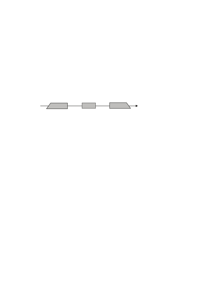
32
( )
B
n
n
T
<
≤
=
1
when
positive,
but
arbitrary
( )
⎣
⎦
(
)
B
n
n
f
b
n
aT
n
T
≥
+
=
when
),
(
/
.
[[This extra condition “n
≥ B” ensures that the recursive equation is well-defined, because then the values
of floor and ceiling fall into {1,2,…,n-1}; indeed then n/b-1
≤ n-1 and n/b≥1 ]]
Then T(n) can be bounded asymptotically as follows.
1) If
)
(
)
(
log
ε
−
=
a
b
n
O
n
f
for some constant
ε>0, then
)
(
)
(
log
a
b
n
n
T
Θ
=
.
2) If
)
(
)
(
log
a
b
n
n
f
Θ
=
, then
)
log
(
)
(
log
n
n
n
T
a
b
Θ
=
.
3) If
)
(
)
(
log
ε
+
Ω
=
a
b
n
n
f
for some constant
ε>0, and if a⋅f(n/b) ≤ c⋅f(n) for some constant c<1, then
))
(
(
)
(
n
f
n
T
Θ
=
.
Intuition behind the theorem:
On recurrence When problem size is at most a constant, then the algorithm must be able to solve the
problem in constant time. Beyond the constant, we can describe the running time of the algorithm in a
recursive fashion. On solution There are three cases. Note that we are “comparing” f(n) with
a
b
n
log
.
When f(n) is “smaller”, then
a
b
n
log
dominates solution; when f(n) is “bigger”, then f(n) dominates
solution; when f(n) is “equal” to
a
b
n
log
, then
n
n
a
b
log
log
dominates solution. There are some other
technical conditions on how much different the functions should be and also on “regularity” of f(n).
Illustration on examples
Example 1 -- positive
Consider recurrence
⎣
⎦
n
n
T
n
T
+
=
)
3
/
(
9
)
(
, for n
≥10, and define T(n)>0 arbitrarily for 1≤n<10 [[so in this range the values
are arbitrary positive – these values are constants]]
So a=9, b=3 and log
b
a=2. So we can use first case, because the exponent in f(n)=n is strictly smaller than
the exponent in
a
b
n
log
, so
)
(
)
(
log
ε
−
=
a
b
n
O
n
f
for a positive
ε=1. So
( )
2
log
)
(
)
(
n
n
n
T
a
b
Θ
=
Θ
=
.
Example 2 -- negative
Consider recurrence
⎣
⎦
n
n
n
T
n
T
log
/
)
3
/
(
9
)
(
2
+
=
,
We still have that
n
n
n
f
log
/
)
(
2
=
is asymptotically smaller than
2
log
n
n
a
b
=
, so we would hope to use
first case. Unfortunately, f(n) is not polynomially smaller. That is it is not the case that n
2
/ log n is not
(
)
ε
−
a
b
n
O
log
. Indeed is cannot be the case that
ε
n
n
c
n
n
a
b
/
log
/
log
2
⋅
≤
for some
ε>0, c>0, and any large
enough n, because for any large enough n, n
ε
outgrows c
⋅log n. So we cannot use Master theorem.
)
(
log
ε
+
Ω
a
b
n
)
(
log
ε
−
a
b
n
O
)
(
log a
b
n
Θ
33
Example 3 -- sophisticated positive
[[Link to what we have done using a lengthy argument, and now we can do quickly using Master
theorem]] We return to the example that we have already studied.
⎣
⎦
4
n
for
),
(
)
4
/
(
3
)
(
3
n
1
for
),
1
(
)
(
2
≥
Θ
+
=
≤
≤
Θ
=
n
n
T
n
T
n
T
so a=3 and b=4. Thus log
b
a < 1. Recall that the Theta in the equation means that instead of the Theta we
have a function f(n)=
Θ(n
2
). So f(n) is asymptotically larger than
a
b
n
log
. So we should be able to use third
case of the Master theorem. The function f may be not “regular”. The idea is to bound T(n) by two other
functions. We can bound f(n) by c
1
n
2
≤ f(n) ≤ c
2
n
2
for large enough n
≥n
0
. Then take B:=max{4,n
0
}, define
U(n) to be the same at T(n) for small n, U(n)=T(n) for 1
≤n<B; and recursively for larger n,
U(n)=aU(n/b)+c
2
n
2
, for n
≥B. Of course then T(n)≤U(n) for all n [[simple induction on n]]. But now c
2
n
2
is
regular, because
a
⋅c
2
(n/b)
2
≤ c⋅c
2
n
2
which is equivalent to
3/16
≤ c⋅
So we can pick c=1/2 which is strictly smaller than 1, as desired. So by Master theorem U(n)=
Θ(n
2
).
Using similar argument we can show that L(n)=aL(n/b)+c
1
n
2
, for n
≥B bounds T(n) from below, and that
by Master theorem L(n) =
Θ(n
2
). Combining these two bounds shows that T(n)=
Θ(n
2
).
[[Master theorem – proof for exact powers, possibly just the first case]]
Summations (arithm, geom, bounds using integrals) [Ch A]
Student should review Section A.2 [[on bounding summations]]
Key ideas are bounding a sum from above by bounding each term from above by the same term
[[hopefully most of them are big]], and bounding a sum from below, by disregarding small terms and
bounding large ones from below by the same term [[hopefully many are large]]
2.2 Quicksort
Today we study another example of divide-and-conquer algorithm that sorts. The algorithm is in some
sense a “mirror” of mergesort. In mergesort the main work is done by merging two already sorted
sequences in the combine phase; while the divide phase is trivial. In the algorithm presented here the main
work is done in the divide phase, while the combine phase is trivial. This algorithm is called quicksort.
Intuition: The idea is to “make the array look more and more sorted overall” [[pick an element called
pivot, partition elements of the segment into these smaller than the pivot and these larger; then call
recursively on the two resulting subsegments – note that pivot is outside of the subsegments]]
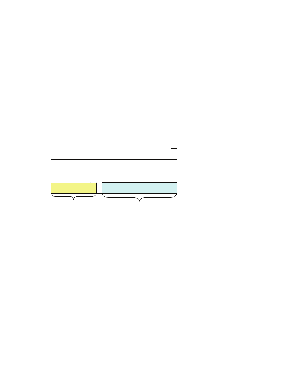
34
Quicksort is an algorithm that has high worst-case running time Θ(n
2
), but low expected running time O(n
log n). The constant hidden by the big-Oh analysis is low, which makes quicksort typically better than
mergesort in practice.
[[show the code of quicksort and partition on a single slide]]
QuickSort(A,p,r)
1 if p<r then
2 q ← Partition(A,p,r)
3 QuickSort(A,p,q-1)
4 QuickSort(A,q+1,r)
The function Partition is the key part of the algorithm. Partition takes segment A[p…r] and rearranges its
elements. Let x be the A[r] at the time of invocation of the function. Then the function rearranges the
elements so that segment A[p…q-1] [[that can be empty]] contains elements at most x, segment
A[q+1…r] [[that can be empty, too]] contains elements strictly larger than x, and A[q] contains x.
A straightforward inductive argument shows that Quicksort is correct [[pending correctness of the
Partition function]]. Our goal now is to implement the Partition function.
Partition(A,p,r)
1
►
We assume that:
p≤r
2 x
← A[r]
3 i
← p-1
4 j
← p
5
while j<r do
6
if A[j]≤x then
7
i ← i+1
8
swap A[j] with A[i]
9
j ← j+1
10 swap A[i+1] with A[r]
11 ►
We want to show that:
p≤i+1≤r and A[p…i] ≤
A[i+1] < A[i+2…r]
12 return
i+1
[[Picture that exemplifies execution; use the picture of the invariant, and show there how elements get
rearranged]]
p
r
x
p
r
≤ x
q
> x
BEFORE
x
AFTER
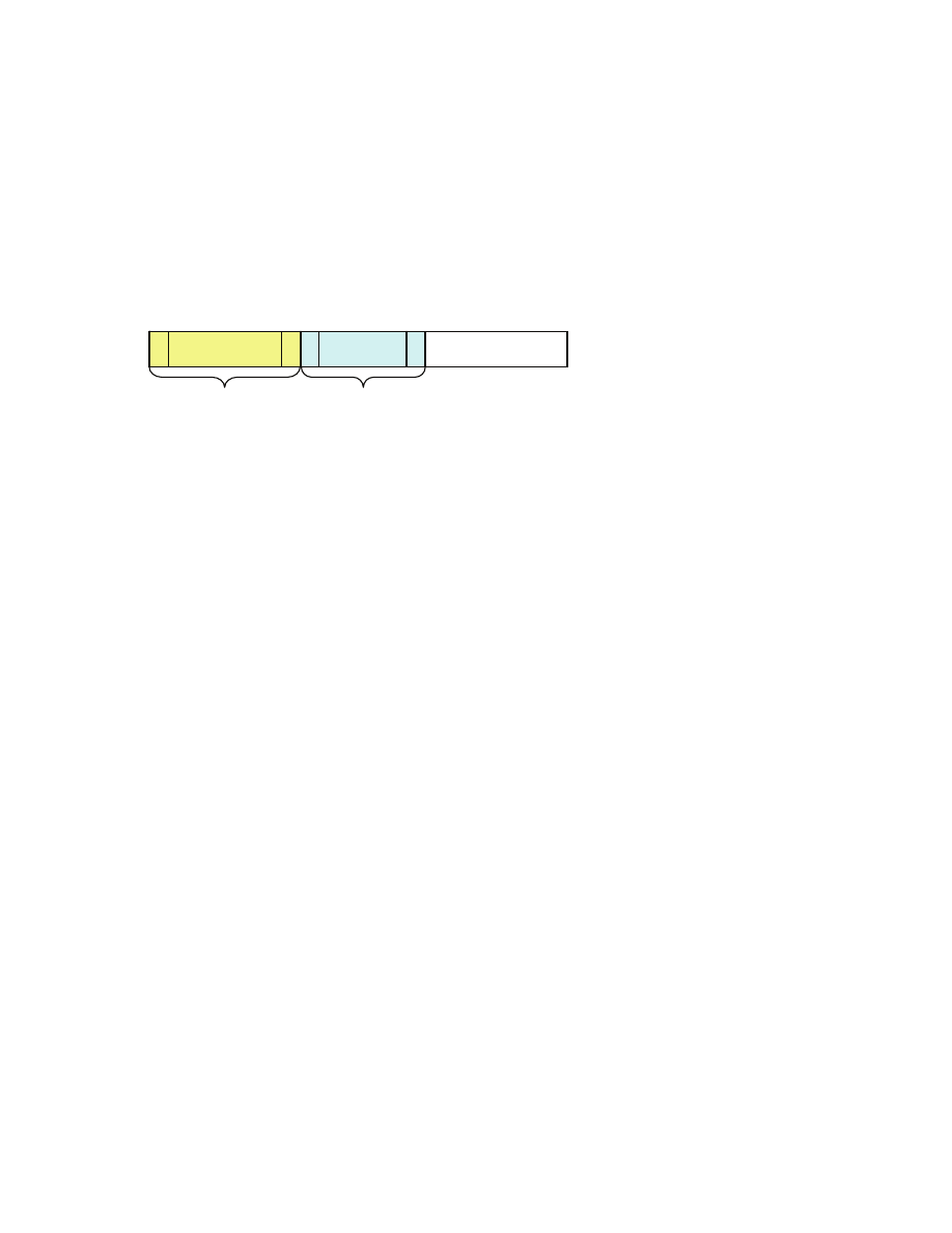
35
Theorem
The Partition algorithm is correct and its running time is Θ(m), where m=r-p+1 is the length of the
segment.
Proof
While loop invariant:
(1)
for all k such that p≤k≤i, A[k]≤x
(2)
for all k such that i+1≤k≤j-1, A[k]>x
(3) p-1
≤ i < j ≤ r
Initialization
(1) is true because i=p-1, so there is no such k
(2) is true because i+1=p and j-1=p-1, so there is no such k
(3) is also true, by the way i and j were initialized
Maintenance
By invariant, j falls within the boundaries of the segment A[p…r]. So A[j] is a valid element.
Suppose that A[j]>x. Then by invariant for all k from i+1 to j-1 it is true that A[k]>x. So for all k from
i+1 to
j
it is true that A[k]>x. So after j has been incremented, (2) holds. (3) holds because j<r before
incrementing j. (1) holds because i is not modified.
Suppose that A[j]≤x. We know that i<j. We have two cases depending on the relationship between i and j.
Case one is when i+1=j (i.e., the
blue
segment is empty). Then by invariant and the assumption, for all k
from p to i
+1
, A[k]≤x. Swapping A[j] with A[i+1] has no effect. The segment from i+2 to j is empty. So
after lines 7 to 9 have been executed, invariant holds. Case two is when i+1<j. Then there is at least one
element in the (
blue
) segment A[i+1…j-1] and any such element is strictly larger than x, by invariant. In
particular, A[i+1]>x. Then swapping A[i+1] with A[j] ensures that for all k from p to i
+1
, A[k]≤x, and for
all k from i
+2
to j, A[k]>x. So after lines 7 to 9 have been executed, the invariant holds.
Termination
We know that when the while loop exits and we are about to execute line 10, the invariant is true. We
conclude that j=r, because by invariant j≤r and the loop guard fails, so indeed j=r. Case one is when i+1=j
[[so the blue segment is empty]]. Then by invariant for all k from p to i A[k]≤x. Swapping A[i+1] with
A[r] has no effect, because i+1=r. Segment A[i+2…r] is empty. Desired statement listed in line 11 holds.
Case two is when i+1<j. Then there is at least one element in the segment A[i+1…j-1], and by invariant
these elements are strictly larger than x. So swapping A[i+1] with A[r] moves this element known to be
strictly larger than x to A[r], while A[i+1] becomes x. Indeed then all elements in A[i+2…r] are strictly
larger than x. By invariant all elements in A[p…i] are at most x. So the desired statement also holds.
Partition halts because j gets incremented in every iteration of the while loop.
█
i
p
j-1
r
≤ x
i+1
> x

36
Theorem
Quicksort sorts.
Proof
An easy inductive argument that uses the fact that the Partition algorithm is correct [[that smaller or equal
elements are moved left and strictly larger right]].
█
[[intuition for running time based on the proportion of split]]
The performance of quicksort depends on how well balanced segment are produced by the partition
function. If the partition function always produces two segments of the same length [[so that q is in the
middle of p and r]], then we roughly get this recurrence on worst case running time
R(n) = 2R(n/2) +
Θ(n)
By the case number two of master theorem, R(n)=
Θ(n log n).
How quick quicksort is when segments are roughly balanced, but not perfectly? Suppose that one is
always 4/5n and the other is 1/5n. Let us perform a rough estimate of worst-case running time using the
technique of recursion tree.
depth
array partitioned into these sizes
costs incurred at this depth only
total
0
n
cn
cn
1
4/5⋅n 1/5⋅n
c⋅4/5⋅n c⋅1/5⋅n
cn
2
4/5⋅4/5⋅n 4/5⋅1/5⋅n 1/5⋅4/5⋅n 1/5⋅1/5⋅n c⋅4/5⋅4/5⋅n c⋅4/5⋅1/5⋅n c⋅1/5⋅4/5⋅n c⋅1/5⋅1/5⋅n
cn
...
...
...
Note that the left part of this tree is deeper, because we multiply by 4/5 [[so the sizes get reduced
slower]], while the right part is shallower, because we multiply by 1/5 [[so the sizes get reduced quicker]].
Note that at depth log
5
n, the rightmost node corresponds to problem of size 1, and all to the left are of
larger size. So beyond this depth some branches of the tree will be empty. At depth log
5/4
n the leftmost
node corresponds to problem of size 1, and there are no other nodes at this depth [[branches got “cut off”
higher in the tree]]. So the maximum depth of the tree is log
5/4
n. So the total cost at each depth is at most
cn [[at some depths, the sum of problem sizes is less than n, because certain branches do not exist at this
depth]], and so the total cost is at most (1+log
5/4
n)cn = O(n log n). So it appears that as long as partition is
roughly balanced, quicksort should have worst-case running time O(n log n).
Worst-case analysis of quicksort
We demonstrate that quicksort is never very slow. That is we show that its worst case running time is
O(n
2
). Let T(n) be the worst case running time of quicksort on a segment of size n. The partition function
splits a segment into subsegments. Recall that one element of the segment is selected as a pivot that
separates the two subsegments, so if the left subsegment has length i, then the right subegment has length
n-i
-1
. Either the left or the right subsegment can be empty, so i ranges from 0 to n-1. When quicksort
invokes itself recursively, the running time on the left subsegment is at most T(i), and on the right
subsegment is at most T(n-i-1), as these are worst case running times on segments of such length. So T(n)
is bounded from above by the maximum across all these running times on subsegments. We recall that
partition has running time
Θ(n), and so its running time can be bounded from above by bn, for any
n
≥n
0
≥1. This discussion gives rise to the following recursive upper bound on T(n).

37
( )
0
0
for
,
n
n
a
n
T
<
≤
≤
( )
( ) (
)
(
)
0
1
0
for
,
1
max
n
n
i
n
T
i
T
bn
n
T
n
i
≥
−
−
+
+
≤
−
≤
≤
We guess that T(n)
≤(a+b)n
2
+a. We use the substitution method to prove that our guess is true. For the
base case, note that the bound is obviously true for all n from 0 to n
0
-1, because of the a in the bound. For
the inductive step, take any n
≥n
0
.
( )
( ) (
)
(
)
(
) (
)(
)
(
)
(
)(
)
(
)
(
)
(
)
(
)
(
)
(
)
(
)
(
)
(
)
(
)
a
n
b
a
n
nb
na
a
n
b
a
n
b
a
b
a
n
b
a
a
bn
a
n
b
a
a
n
n
b
a
bn
a
n
b
a
bn
a
i
n
b
a
i
b
a
bn
i
n
T
i
T
bn
n
T
n
i
n
i
+
+
≤
≥
≤
−
−
+
+
+
+
+
=
+
−
+
+
+
+
+
+
=
+
+
−
+
+
=
+
−
+
+
≤
≤
+
−
−
+
+
+
+
≤
≤
−
−
+
+
≤
−
≤
≤
−
≤
≤
2
2
2
2
2
2
2
1
0
1
0
}}
1
since
{{
2
2
2
1
2
2
1
2
2
1
}}
boundry
at the
maximized
t
coefficien
positive
ith
function w
quadratic
{{
2
1
max
}}
assumption
inductive
{{
1
max
But notice that the function f(n)=(a+b)n
2
+a is O(n
2
).
Corollary
The worst-case running time of quicksort is O(n
2
).
█
Note that we can use the same technique to derive a lower bound on the best-case running time. We
formulate a recursive equation where instead of maximizing [[as we did for T(n)]], we minimize across
the value of i.
2.3 Randomized quicksort
The problem with quicksort is that we may be unlucky and receive an input array such that partition
always creates very unbalanced subsegments. This occurs, for example, when the array is already sorted
and contains distinct elements, because then A[r] is the largest in the segment, so q will be set to r, and the
content of the segment will not change, so in the recursive call again q will be set to the rightmost tip of
the segment, and so on. Thus the problem is when we pick as the pivot either the largest or the smallest
element in the segment. To alleviate this problem, we randomly pick an element from the segment, and
partition the segment around the element, hoping that with high probability we avoid picking such
extreme elements, and as a result on average the partitions should be well-balanced.

38
RandomizedPartition(A,p,r)
1 i
← element selected uniformly at random from
{p,...,r}
2 swap A[r] with A[i]
3 return
Partition(A,p,r)
RandomizedQuickSort(A,p,r)
1 if p<r then
2 q ← RandomizedPartition(A,p,r)
3 RandomizedQuickSort(A,p,q-1)
4 RandomizedQuickSort(A,q+1,r)
Such algorithm is called a randomized algorithm, as its behavior is not determined solely by the input,
but also by the random choices that the algorithm makes as it executes. When we run the algorithm on the
same input over and over again, the algorithm may compute differently each time we run it. We can then
average the running time across these different runs [[for the same input]]. The hope is that the average is
lower than
Θ(n
2
). [[Strictly speaking, we would take the sum across all possible ways the algorithm can
execute on this input, of the running time of the execution, times the probability that the execution
occurs.]]
Theorem
The expected running time of Randomized quicksort is O(n log n), when invoked on any array with n
distinct elements.
█
Proof of expected running time of Randomized quicksort
How quick is the Randomized Quicksort (RQ) on average? Intuition tells us that on average, partitions
should be well-balanced because we pick pivot uniformly at random, and so the depth of recursion tree
should be O(log n). Since each level of the tree contributes O(n) to the running time, the total running
time should be O(n log n) on average. Today we will start analyzing RQ, with the ultimate goal of
showing that expected running time of randomize quicksort is O(n log n). At the same time, you will see
an example of techniques used to analyze a randomized algorithm [[randomized algorithms are usually
easy to formulate but hard to analyze]].
Probability theory review [[informal review]]
Consider a random experiment with outcomes from a set
Ω. A random variable X is a function from Ω to
the set of real numbers. [[it assigns a number to each outcome]]. In the remainder, the set
Ω of outcomes
will be finite.
Example
Let the random experiment be tossing a fair coin. There are two outcomes of the experiment: coin comes
up heads, coin comes up tails. Let X be a random variable equal to the number of heads that come up in
this experiment.
For a given random variable X, we can consider the probability Pr[X=v] that X is equal to v. How to
calculate this probability? Each outcome has a probability of occurring, we can take all outcomes for
which X is equal to v, and sum up their probabilities. Let V be the set of values that X takes. Expected
value of X is the summation across the values that X takes, of the value multiplied by the probability that
X is equal to the value.

39
[ ]
[
]
∑
∈
=
⋅
=
V
v
v
X
v
X
E
Pr
Example
In our example, the probability of head is 1/2 and of tails is also 1/2. So Pr[X=0] = 1/2 and Pr[X=1] = 1/2.
The set of values V={0,1}. And expected value of X is E[X] = 0
⋅1/2 + 1⋅1/2 = 1/2. So we expect to see
half heads on average.
There is a tool that simplifies the calculation of expected value. Consider any two random variables X and
Y defined over the same random experiment. Then
E[X+Y] = E[X] + E[Y].
This fact is called linearity of expectation. It is a very useful fact when analyzing randomized algorithms,
such as randomized quicksort.
Proof of linearity of expectation
Let V
X
be the set of values take by X, and V
Y
by Y. Let Pr(x,y) be the probability that X is equal to x and
Y to y in this experiment. Then
[
]
(
) ( )
( )
( )
( )
( )
∑ ∑
∑ ∑
∑
∑
∑
∈
∈
∈
∈
∈
∈
∈
∈
∈
∈
+
=
+
=
+
=
+
Y
X
X
Y
Y
X
Y
X
Y
X
V
y
V
x
V
x
V
y
V
y
V
x
V
y
V
x
V
y
V
x
y
x
y
y
x
x
y
x
y
y
x
x
y
x
y
x
Y
X
E
,
Pr
,
Pr
,
Pr
,
Pr
,
Pr
But
( )
( )
x
y
x
Y
V
y
Pr
,
Pr
=
∑
∈
and
( )
( )
y
y
x
X
V
x
Pr
,
Pr
=
∑
∈
So E[X+Y] indeed equals to E[X] + E[Y].
█
Example
Let the random experiment be n tosses of n fair coins. Let X
i
be equal to 1 if coin number i comes up
heads, and 0 if it comes up tails. What is the expected number of heads in this experiment? The number of
heads is X
1
+…+X
n
. By linearity of expectation
E[X
1
+…+X
n
] = E[X
1
] + … + E[X
n
] = n/2 .
Analysis
With this review of probability theory, we begin analysis of randomized quicksort. Our goal for now is to
relate the running time of the algorithm to the number of comparisons that the algorithm makes.
[[show the code as a reminder --- indicate that to code of the algorithm got converted so that the algorithm
is a comparison sort]]
Let us fix the array A. Let us execute RQ on this array, and afterwards inspect the execution. What was
the running time T i.e., how many primitive operations were executed? Each call to RQ results in at most

40
a constant number of primitive operations, excluding the cost of the call to Partition. So let us bound from
above the number of times RQ was invoked.
Lemma
For any n≥0, when Randomized Quicksort is called on an array of length n, then the procedure
RandomizedQuicksort can be invoked at most 3n+1 times [[until the algorithm halts]].
Proof
We inspect the code of RQ. Each time the function RandomizedQuicksort is called on a segment of length
2 or more, the function Partition is called. Inside this function a pivot is selected, and elements of a
segment are partitioned around the pivot. None of the two resulting segments contains the pivot. Then RQ
is called recursively on each of the two segments. Thus an element that is selected as a pivot cannot be
selected as a pivot again, simply because it is excluded from segments passed on to the recursive calls.
There are at most n elements that can be selected as a pivot. Therefore, in any execution of RQ, there can
be at most n invocations of RQ on segments of length 2 or more. How about invocations on segments of
length 1 or less? How many can there be? We first notice under what circumstances an invocation on such
a short segment can happen. There are two cases: the invocation is the initial invocation (because n is 1 or
0), or the invocation is a recursive call performed by procedure RQ. There can be at most 1 call of the
first type, because any such call does not make any recursive calls [[condition “p<r” is false]]. How about
the other type? These can be made only by invocations of RQ on segments of length 2 or more. Any such
invocation can make at most 2 invocations on segments of length 1 or 0, and invocations on such short
segments cannot make any more because inside them “p<r” is violated. But there are at most n
invocations of RQ on segments of length 2 or more. So there are at most 2n invocations on segments of
length 1 or 0. So the total number of invocations of RQ [[on short and long segments]] is at most 1+3n.
█
Now, how about the number of primitive operations performed inside a single invocation to Partition? It
is also a constant, except for the body of the while loop [[lines 6 to 9]]. This body can be executed
multiple times. Whenever the body of the while loop is executed, two elements of array A are compared
[[line 6]]. So if we let X denote the total number of comparisons of elements of A during the execution
[[from all invocations to Partition]], then the running time T was at most c·(1+3n+X). This is summarized
below.
Lemma
The time T of any execution of RQ is at most c·(1+3n+X), where X is the total number of comparisons of
elements of A made during this execution, and c>0 a constant.
We can now consider all possible ways in which the algorithm can be executed on this array A. These
ways are determined by the random choices performed by the algorithm [[random selection of integers]].
Let r be the random choices performed during an execution [[this r can be thought of as a sequence of
numbers]]. Given r, and the input A, the execution is determined [[there is not randomness any more, as
numbers r have been fixed]]. Let T(r) be the running time and X(r) the number of comparisons. So the
lemma that we just showed states that
T(r)
≤ c·(1+3n+X(r)) .
We can calculate the probability Pr(r) that the random choices made are equal to r. Thus X and T can be
treated as random variables. Therefore, expectations are also related
[ ]
( ) ( )
( )
(
)
(
) ( ) (
)
[ ]
X
E
c
n
c
r
r
X
n
c
r
r
T
T
E
r
r
⋅
+
+
=
⋅
+
+
≤
⋅
=
∑
∑
3
1
Pr
3
1
Pr

41
We want to find a bound on the expected value of T. Hence it is enough to find E[X]. If we are able to
show that E[X] is O(n log n), then E[T] is also O(n log n), because the linear summand c(1+3n) will get
subsumed by n log n.
The remainder of the analysis bounds E[X] from above.
We assume that all elements of A are distinct [[this is necessary; if all are the same, then expected running
time is
Θ(n
2
); RQ can be easily modified to alleviate the problem]]. Let z
1
<z
2
<…<z
n
be these elements.
The idea is that we can relate X to the probability that z
i
and z
j
are compared. We can rewrite X as [[we
take all pairs i<j]]
∑ ∑
−
=
+
=
=
1
1
1
]]
to
compared
is
times
of
[[number
n
i
n
i
j
j
i
z
z
X
Notice that z
i
and z
j
can get compared at most once during the entire execution, as they are compared only
when one of them is a pivot, and then this pivot is never again compared to the other in this execution.
So we can rewrite X as
∑ ∑
−
=
+
=
⎭
⎬
⎫
⎩
⎨
⎧
=
1
1
1
compared
not
if
0
to
compared
is
if
1
n
i
n
i
j
j
i
z
z
X
Let X
i,j
be a random variable equal to 1 when z
i
is compared to z
j
, and to 0 if they are not compared [[we
check if they are compared or not during the entire execution of the algorithm]]. Then
∑ ∑
−
=
+
=
=
1
1
1
,
n
i
n
i
j
j
i
X
X
.
We want to calculate the expected value of X. We can use linearity of expectation to show that
[ ]
[ ]
[
]
[
]
(
)
[
]
∑ ∑
∑ ∑
∑ ∑
∑ ∑
−
=
+
=
−
=
+
=
−
=
+
=
−
=
+
=
=
⋅
+
⋅
=
=
⎥
⎦
⎤
⎢
⎣
⎡
=
1
1
1
1
1
1
1
1
1
,
1
1
1
,
to
compared
is
Pr
to
compared
not
is
Pr
0
to
compared
is
Pr
1
n
i
n
i
j
j
i
n
i
n
i
j
j
i
j
i
n
i
n
i
j
j
i
n
i
n
i
j
j
i
z
z
z
z
z
z
X
E
X
E
X
E
=
Our next goal will be to find the probability that z
i
is compared to z
j
[[during the entire execution when
given the fixed A as the input]].
What is the probability that z
i
is compared to z
j
? We shall see that z
i
and z
j
are compared in a very specific
situation. Let Z
i,j
be the set {z
i
,z
i+1
,…,z
j
}. It is convenient to think that i and j are fixed (i<j).
Lemma 1
Consider any moment of any execution of the randomized quicksort. If every pivot that has been selected
so far does not belong to Z
i,j
, then Z
i,j
is included in a single segment at this moment.

42
Proof
Let us inspect the state of the algorithm at this moment. If no pivot has been selected yet, then there is a
single segment that includes all elements, and so the entire Z
i,j
as well. So in this case the lemma holds.
Suppose that at least one pivot has been selected so far. Let z
i,1
,z
i,2
,…,z
i,k
be these k pivots. Let us inspect
the state of the algorithm and what segments have been created so far [[the picture here has k=2]].
There are exactly k+1 segments at this moment. By the property of the algorithm, segment 0 contains all
elements strictly smaller than z
i,1
, segment k contains all elements strictly larger than z
i,k
, and any other
segment m contains all elements strictly larger than z
i,m
but strictly smaller than z
i,m+1
. Can it be the case
that Z
i,j
is not included in one of the segments? If Z
i,j
“sticks out” of a segment [[contains an element other
than from a single segment]], then since Z
i,j
is the set of the elements with rank i through j, so Z
i,j
would
have to contain one of the pivots, which we assumed was not the case. Thus Z
i,j
must be included in a
single segment.
█
Our goal now is to calculate the probability Pr[ the first pivot selected from Z
i,j
is either z
i
or z
j
]. As a
result of this lemma as long as the algorithm is selecting pivots outside of Z
i,j
, the set Z
i,j
stays inside a
segment (this may be different segment at different points of time). There is always a time when a pivot
that belongs to Z
i,j
is selected. So at the first such moment, this Z
i,j
is included in a single segment. But the
selection of a pivot in any segment is done uniformly at random. Hence the chances that any particular
element of Z
i,j
is selected as a pivot are 1 divided by the number of elements in Z
i,j
, which is 1/(j-i+1). The
selection of z
i
as the first pivot from Z
i,j
is mutually exclusive from the selection of z
j
as the first pivot
from Z
i,j
(recall that i<j) [[either one is selected or the other, but never both can be selected; because we
focus on the selection for the first time]]. This proves the following fact
Fact 1
Pr[ the first pivot selected from Z
i,j
is either z
i
or z
j
] = Pr[the first is z
i
] + Pr[the first is z
j
] = 2/(j-i+1) .
Lemma 2
Elements z
i
is compared to z
j
if and only if the first pivot selected from Z
i,j
is either z
i
or z
j
.
Proof
We first show when z
i
cannot be compared to z
j
. Consider the first moment when a pivot is chosen that
belongs to Z
i,j
. By Lemma 1, the set Z
i,j
was included in one of the segments that existed right before that
moment, and any pivot selected before then was not in Z
i,j
. But this means that z
i
could not have been
compared to z
j
, neither z
j
to z
i
, because any comparison involves a pivot [[by the property of the partition
function]], and neither z
i
nor z
j
was a pivot. Thus z
i
can be compared to z
j
only after a pivot is selected
that belongs to Z
i,j
. If this pivot x selected at this moment is neither z
i
nor z
j
, then z
i
<x<z
j
and so the
partitioning function will put z
i
and z
j
into separate segments without comparing z
i
to z
j
[[only to x]], and
z
i
will never be compared to z
j
later. If this pivot is either z
i
or z
j
, then they will get compared.
█
As a result of Lemma 2 and Fact 1, the probability that z
i
is compared to z
j
is exactly 2/(j-i+1).
Hence
< z
i,1
<
segment 0
segment 1
< z
i,2
< segment 2
43
∑∑
∑∑
∑ ∑
∑ ∑
−
=
=
−
=
−
=
−
=
+
=
−
=
+
=
=
<
+
=
+
−
=
=
1
1
1
1
1
1
1
1
1
1
1
1
)
log
(
2
1
2
1
2
]
to
compared
is
Pr[
]
[
n
i
n
k
n
i
i
n
k
n
i
n
i
j
n
i
n
i
j
j
i
n
n
O
k
k
i
j
z
z
X
E
The argument presented so far proves the following theorem
Theorem
For any array of n distinct numbers, the expected running time of randomized quicksort on the array is
O(n log n).
2.4 Lower bound on the time of sorting
So far we have seen one algorithm that sort in time
Θ(n log n) in the worst-case: mergesort. One may
wonder, is it possible to sort faster? In general when we try to solve a computational problem, we may
come up with an algorithm that has certain worst-case running time, and we may be wondering if there is
an even faster algorithm. Can we always find a faster algorithm? It turns out that sometimes it is just
impossible to find a faster algorithm, because no such algorithm exists! Today we will see an example of
such impossibility result. We will see that any deterministic algorithm that sorts using comparisons must
have worst-case running time at least
Ω(n log n), when sorting an array of length n. This is an amazing
fact. The mergesort sorting algorithm is asymptotically optimal.
Let us define a class of algorithms. Later on, we will show that any algorithm in our class has worst-case
running time
Ω(n log n). Let us inspect the structure of mergesort to motivate the definition of our class.
In the code of the algorithm, we swapped elements of array A, or stored them in temporary variables.
This, however, is not necessary. The algorithm does not have to read the values of elements of A at all.
We can easily rewrite the algorithm so that it only accesses elements of A indirectly through questions of
the kind “A[i]
≤A[j] ?” that compare elements of the array, but the algorithm does not read the values of
the elements. So as the algorithm executes, it occasionally compares elements of array A:
……
Is A[i]
≤A[r] ?
……
Eventually, the algorithm decides on the way to reorder A so that the resulting array is sorted and the
algorithm halts. In other words, the algorithm takes an array A[1…n] as an input, then the algorithm
compares pairs of certain elements of A in one of the following ways
• A[i] > A[j]?
• A[i] < A[j]?
• A[i] = A[j]?
• A[i] ≤ A[j]?
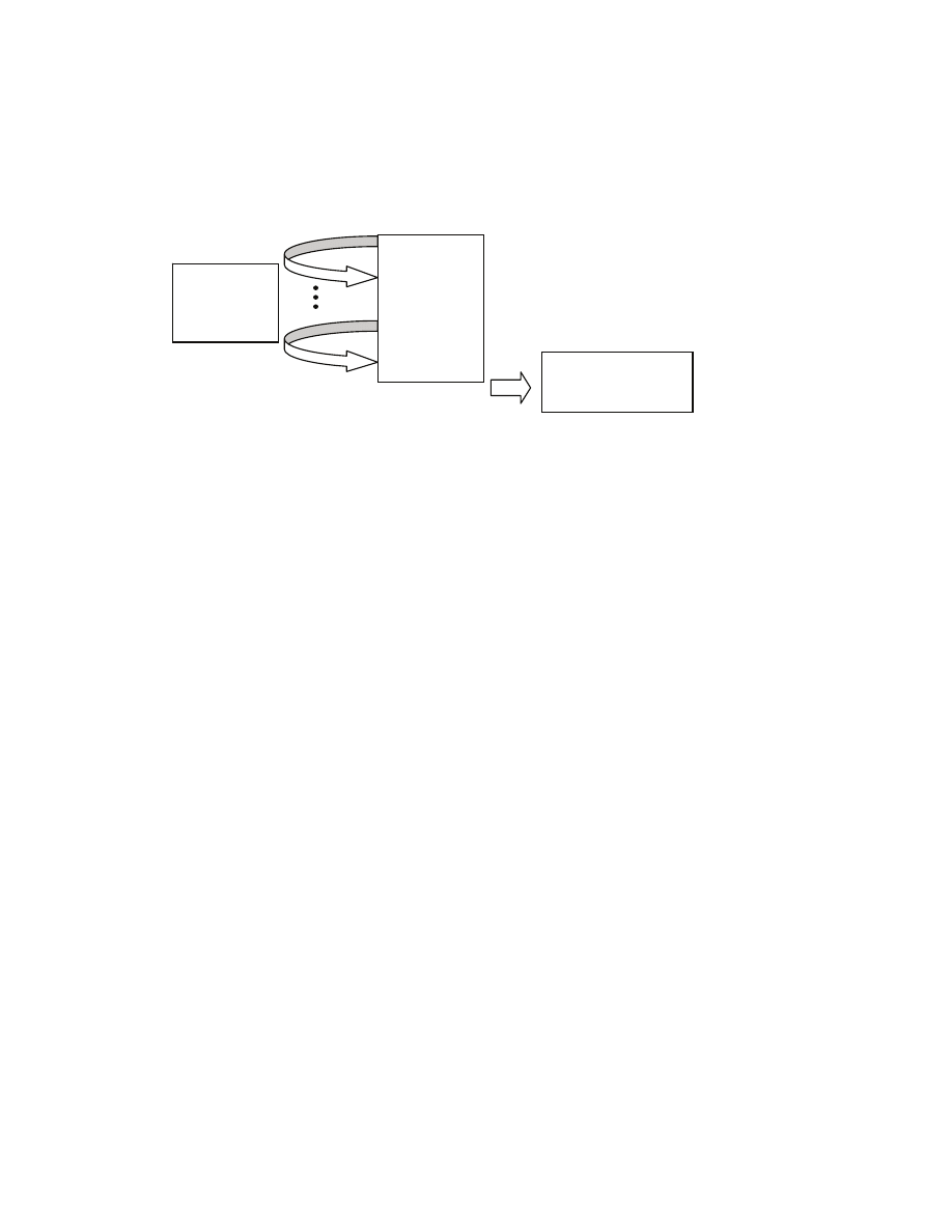
44
• A[i] ≥ A[j]?
and finally outputs n distinct numbers p
1
,…,p
n
from {1,…,n} that describe how the elements of A can be
reordered so that the reordered sequence is sorted, that is A[p
1
]
≤ A[p
2
]
≤ … ≤ A[p
n
]. Such algorithm is
called comparison sort (because it compares elements).
We can think of the execution of comparison sort as a conversation between the algorithm and the array.
There is an array A of n numbers from {1,…,n}. The algorithm can ask the array questions of the five
types. The array answers either “Yes” or “No” to each question. After a sequence of Q&A, the algorithm
must determine a way to reorder A so as to make the reordered elements increasing. In other words, the
algorithm issues a question q
1
to which the array gives answer a
1
, then the algorithm issues question q
2
, to
which the array gives answer a
2
, and so on until the algorithm issues the last question q
k
number k to
which the array gives an answer a
k
, and then the algorithm decides on an reordering and returns a
sequence of n distinct numbers from {1,…,n} that describe how to reorder the array to make it sorted.
Suppose that we are given a deterministic comparison sort that, given any array of n integers, asks exactly
one question and then decides. How many different decisions can the algorithm make? Note that since the
algorithm is deterministic, the question is the same, no matter what array of n integers is given. The
answer can be either Yes or No. If Yes, then the algorithm will decide on something, call it D
1
. Now
notice that no matter what array was provided, as long as the answer is Yes, the decision is the same D
1
.
Similarly, if the answer is No, then the algorithm decides on something, call is D
0
. Again, no matter what
array is provided, as long as the answer is No, the algorithm will decide on the same D
0
. So there are at
most two different decisions. In general, if the algorithm always asks h questions, then there can be at
most 2
h
different decisions.
The following amazing fact states that conversations with different arrays must be different.
Lemma
Pick any deterministic comparison sort. Let A and A’ be two different arrays, each containing n distinct
numbers from {1,…,n} [[so arrays are permutations]]. Let S be the sequence of answers generated until
the algorithm decides on a reordering when “conversing” with A, S=a
1
, a
2
, …, a
k
, and S’ when
“conversing” with A’, S’=a’
1
, a’
2
, …, a’
k’
[[note that these sequences of answers may have different
lengths i.e., k may be different from k’]]. Then the two sequences must be different, S
≠S’.
Proof
Since A is different from A’, the algorithm must decide on different output sequences. Assume, by way of
contradiction, that the sequences are the same S=S’ [[in particular they have the same number of answers
k=k’]]. Recall that the algorithm does not “see” the elements of the array; it knows about the array exactly
as much as it has learned from questions and answers. Let us trace how the state [[the variables of the
program]] of the algorithm changes as the algorithm issues questions and receives answers. Let us first
Algorithm
Input array
2,3,1,4
Output sequence
3,1,2,4
compare
result
compare
result

45
focus on the “conversation” about A. The algorithm always starts in an initial state V
0
[[that describes
how the variables are initialized]]. Then the algorithm issues a question q
1
and receives an answer a
1
,
which brings the algorithm to a state V
1
. In general, after issuing a question q
i
and receiving an answer a
i
,
the algorithm reaches a state V
i
. So the final state of the algorithm is V
k
, where the algorithm decides on
some output. The algorithm is deterministic, so now when conversing with A’, it starts in the same state
V
0
, so asks the same first question q
1
, and by assumption it receives the same response a
1
, which brings it
to the same state V
1
. So the second question is the same q
2
!!!! But again by assumption the answer is a
2
,
so the third question is q
3
. We can see that this pattern repeats, leading to state V
k
after k question. So
when invoked on A’, the algorithm must decide on the same output as when invoked on A. But this is a
contradiction, because we know that the decisions of the algorithm must be different, because arrays A
and A’ are different. This completes the proof.
█
Theorem
Any deterministic comparison sort must have running time at least
Ω(n log n), where n is the number of
elements to be sorted.
Proof
Suppose that the sorting time of any array of numbers from {1,…,n} is at most m. This means that the
algorithm can ask at most m questions. So the algorithm must decides in 0 or 1 or 2 or 3 or … or m
questions. We observed that when algorithm decided in h questions, it can make at most 2
h
different
decision. So the algorithm can make at most 2
0
+ 2
1
+ 2
2
+…+2
m
≤ (m+1)⋅(2)
m
different decisions. There
are n! [[n factorial]] different arrays of distinct numbers from {1,…,n}. By the Lemma, when the
algorithm “converses” about an array, it produces a distinct sequence of answers [[different from the one
produced when conversing about a different array]]. This sequence must be of length m at most. Thus
((the number of arrays of n distinct numbers from {1,…,n}))
≤
((number of sequences of answers of length at most m that the algorithm can generate))
but the latter is bounded from above by (m+1)2
m
, and so
n!
≤ (m+1)2
m
Now we can take log of both sides
log (n!)
≤ log( (m+1)2
m
)
so
(log 1) + (log 2) + (log 3) + (log 3) + … + (log (n-1)) + (log n)
≤ log( (m+1)2
m
)
But in the summation, at we have least n/2-1 summands in the tail, each of which has value at least
log(n/2), so
(n/2-1) log n/2
≤ m + log(m+1) ≤ 2 m
So m is
Ω(n log n).
█
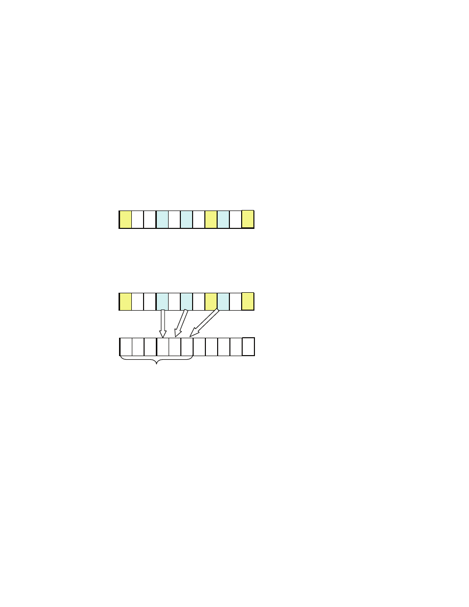
46
2.5 Countingsort
Can we sort faster than
Θ(n log n)? For example, can we sort as fast as O(n)? The lower bound that we
showed says that if we use only comparisons to gain information about the elements that we need to sort,
and we must be able to sort any sequence, then in the worst-case
Ω(n log n) time is necessary to sort.
How about if we do not use comparisons and decide to sort only specific sequences? It turns out that then
we can sort in O(n) time in the worst-case! One such algorithm is called countingsort. We will study this
algorithm today.
“How to beat the lower bound? Impossible? Not really. Do not use comparisons, use something else!”
The key idea of the countingsort algorithm is to use the values of the elements [[do not compare
elements]] and assume that there are not too many of these values. Suppose that you have an array
A[1…n]. Pick an element from this array, say equal to 2.
This element can occur several times in the array (blue). Let c be the number of elements in the array
smaller or equal to 2 (blue and yellow). In our example array A, we have c=6 elements equal to at most 2
(these are 0,0,1,2,2,2). If we know c, then we can immediately place the three elements equal to 2 at the
appropriate locations in the array B that will contain sorted elements of A:
These three elements should be placed at output locations B[c-2], B[c-1] and B[c] in the order from left to
right. If we perform this placement for all distinct elements of A, then B will contain all elements of A in
a sorted order. Moreover, any two equal elements from A (such as equal to 2 in the example), will occur
in B in the order in which they occurred in A. A sorting algorithm that preserves order of equal elements
is called stable.
The issue that remains to be solved is how to quickly count the number of elements equal to at most a
given element, for any element of A. We assume that elements of the array fall into the set {0,1,…,k} – so
there are k+1 possible choices only. This is an important restriction that will make countingsort run fast.
x
input A:
2
2
2
1
0
0
9
8
8 6
7
x
input A:
2
2
2
1
0
0
9
8
8 6
7
output B:
2
2
2
c=6

47
CountingSort(A,B,k)
1 ►
Reset counters
2 for
i
← 0 to k do
3 C[i] ← 0
4 ►
Count number of elements that have a given value
5 for
j
← 1 to length[A]
6 C[A[j]] ← 1+C[A[j]]
7 ►
Count number of elements that have at most a
given value
8 for
i
← 1 to k
9 C[i] ← C[i-1]+C[i]
10 ►
Place elements at the right locations in B
11 for j ← length[A] downto 1
12 B[C[A[j]] ← A[j]
13 C[A[j]] ← -1 + C[A[j]]
Theorem
CountingSort sorts and is stable. Its running time is O(k+n). The algorithm uses O(n+k) memory.
Proof
Correctness follows from the earlier discussion on how elements should be placed in array B so that B
contains elements of A in a sorted order, and that any two elements of A with the same value appear in B
in the same order. Each of the three for loops iterates at most k+1 or at most n times. We need extra
memory of size k+1 for the array C and of size n for the array B.
█
So note that as long as elements of the array are from the set {0,1,…,k} and k=O(n), countingsort sorts in
linear time. Relate this result to Mergesort and Quicksort that have no restrictions on how big the values
of elements are [[as long as it is reasonable to assume that comparison of any two elements takes constant
time]], so k could be as large as n
2
, and we could sort such elements in O(nlog n) using Mergesort, while
countingsort would need
Θ(n
2
) time [[and space]], which is asymptotically more.
2.6 Radixsort
The algorithm that we studied recently, countingsort, has running time
Θ(n+k), where {0,1,…,k} is the
range of values in the array. This is particularly good when k is O(n), because then running time is
Θ(n),
which is asymptotically optimal. However, when k is very large compared to n, e.g., k=n
2
, then
countingsort is slower than mergesort or quicksort. Today, we will see how to use countingsort to design
a fast sorting algorithm whose running time does not increase so fast as k increases.
The algorithm called radixsort uses the following approach. It takes numbers, each composed of d digits.
Then it first sorts the numbers with respect to the least significant digit. Then with respect to the second
digit, then with respect to the third, and so on and finally it sorts numbers with respect to digit number d.
Example
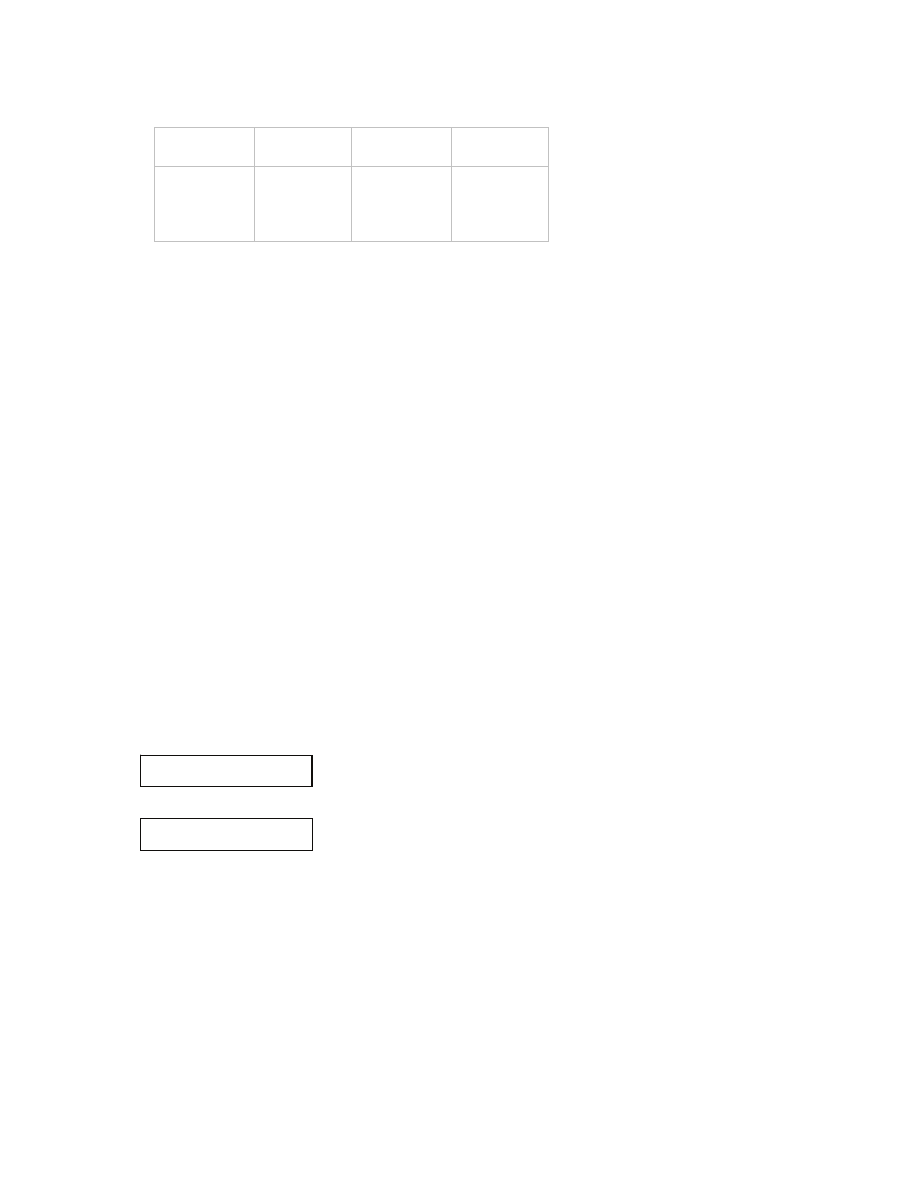
48
Focus on the
first digit
result
after sorting
Focus on the
second digit
result
after sorting
(2,
3
)
(2,
4
)
(1,
5
)
(3,
1
)
(3,
1
)
(2,
3
)
(2,
4
)
(1,
5
)
(
3
,1)
(
2
,3)
(
2
,4)
(
1
,5)
(
1
,5)
(
2
,3)
(
2
,4)
(
3
,1)
Remarkably, as long as each sorting is stable [[stable means that the order of equal elements is not
changed by the sorting]], the resulting sequence is sorted. In particular, in the example above, in the
second sorting it is important to keep (2,3) above (2,4). The reason why radixsort is correct will be
explained in a moment.
[[show the code and explain again how it works]]
RadixSort(A,d)
1 for
i
← 1 to d do
2 sort A with respect to digit i using a stable
sort
Lemma
At the end of each iteration, the elements of A are sorted with respect to the least significant i digits
(digits 1 through i).
Proof
The proof is by induction. The base case is trivial. The first iteration sorts elements of A with respect to
the least significant digit. Thus at the end of the first iteration the elements of A are sorted with respect to
the least significant digit. Assume that at the end of iteration i
≥1 elements of A are sorted with respect to
the least significant i digits, that is digits 1 through i. Let us see the state of A at the end of iteration i+1.
Between then and now, A gets sorted with respect to digit number i+1 in a stable manner. Focus on A at
the end of iteration i+1. Is it sorted with respect to the least significant i+1 digits? Pick any two elements
x and y of A. If they differ on digit i+1, then they are sequenced in A appropriately, because A just got
sorted with respect to digit i+1. So suppose that they have the same digit i+1. (in the figure x=y=5)
But then they should be sequenced in A with respect to digits i through 1. Specifically, the element whose
digits i through 1 represent a smaller number should occur in A earlier. But this is indeed how x and y
were ordered right before A was sorted with respect to digit i+1. But the sorting that was just performed is
stable. So x and y are still sequenced as desired. This completes the inductive step and the proof.
█
~~~~~
5
3 2 9
~~~~~
5
4 6 1
digits
d ...... i+1 i ..... 1

49
Theorem
Radixsort sorts. Its worst-case running time is
Θ(d⋅(n+k)) when each digit has values from {0,1,…,k} and
countingsort is used to sort with respect to each digit, an we use a pointer representation of numbers of A
[[so that when we need to swap two numbers, we actually only swap pointers to the numbers, and not the
d digits]]
Proof
Follows directly from the Lemma and a bound on running time of countingsort.
█
Application
Computers have a natural representation of numbers in binary. Suppose that we are given n numbers each
with b bits. We can partition b bits into chunks of r bits each; so there will be b/r chunks. In each iteration
of radixsort, we sort with respect to a chunk. So such algorithm will have worst-case running time
Θ(b/r
(n+2
r
)). Now we can select various r that may impact this bound on time. How big should r be to achieve
the lowest running time? If each element of array A has value at most n (that is b
≤log n), then best
radixsort is obtained by sorting on all bits (in one iteration, so r=b) in time
Θ(n). If each element of A can
be larger than n, and as large as 2
b
, then best radixsort is obtained by partitioning into chunks of size r=
log n bits (using b/log n iterations) in time
Θ(bn/log n). [[Here we assume that indexing array through b
bits takes constant time]]
3 Dynamic programming
Dynamic programming is a technique of solving computational problems. It is similar to divide-and-
conquer. Given a problem, we divide it into subproblems, and solve them recursively. Unlike divide-and-
conquer, in dynamic programming subproblems may overlap, and thus we may generate multitude of
subproblems as we keep expanding the recursive calls. This may lead to exponential running time. A key
idea of dynamic programming is to remember solutions to subproblems in a table [[or array]] so that they
do not need to be recomputed by the various recursive calls. Then it is possible to achieve polynomial,
and not exponential, running time. We will subsequently study several examples of application of the
dynamic programming technique to solving computational problems, and see details of the intuitive ideas
of the technique that we have just mentioned.
Dynamic programming is used to solve optimization problems. For example, we have a factory that
produces cars on assembly lines, each line is composed of stations, each station has a certain processing
time, and a certain time is needed to transfer chassis from a station to a station. What we want to find is
how to route a chassis through the assembly lines to minimize the assembly time. In general, an
optimization problem consists of an input [[here the description of the factory]], there are several possible
solutions [[here ways to route a chassis through the assembly lines]], each solution has a value [[routing
time]], and we seek a solution that minimizes the value [[lowest possible routing time]]. Alternatively, for
some optimization problem, we may seek a solution that maximizes the value [[e.g., when we deal with a
financial optimization problem]]. Such solution is called an optimal solution [[when it is clear from the
context whether we mean maximum or minimum]].
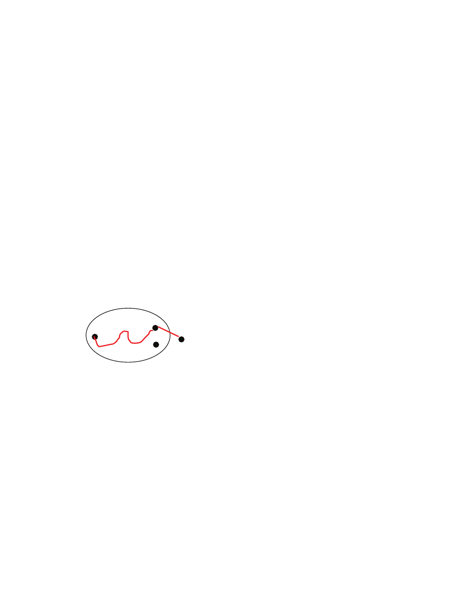
50
3.1 Assembly-line scheduling
Picture 15.1 from CLRS.
State the problem: two lines each has n stations, entry times from the starting point e
1
and e
2
, processing
times a
1,j
and a
2,j
at stations, exit times to the exit point x
1
and x
2
, “cross” transfer times from a station j to
the next t
1,j
, t
2,j
. on the other line Describe how processing is done: cars need to be on consecutive stations,
normally a car sticks to line 1 or to line 2, but sometimes there is a rush order. Our goal is to find out how
quickly we can process a rush order. Possible solutions: subsets of stations; show an example; a route, and
routing time.
Trivial approach
Use “brute force” method -- check all possible 2
n
routes, find routing time of each in O(n). Total is Ω(2
n
)
-- too time consuming to calculate for large n.
We now develop a much faster algorithm. We will do this in a few steps.
1) Structure of an optimal solution
[[we work from the back]]
Pick a route that minimizes routing time. It exist either through the first line on station S
1,n
or the second
line on station S
2,n
. For the time being let us assume that it is S
1,n
[[the analysis is symmetric in the case of
S
2,n
]]. So we can depict the situation as follows, where red corresponds to an optimal route.
Let us focus on the chassis moving along the route, and let t be the time when the processing at station
S
1,n
completes [[in this route]]. We can consider all possible ways to get from the start through S
1,n
, and
let t’ be the fastest possible time. Now the key observation is that t=t’. Indeed, t
≥t’, because t’ is the
fastest way to get through S
1,n
, and so our route cannot get there strictly faster. It cannot be the case that
t>t’. If it was the case, then we could use this route that gets us from start through S
1,n
in time t’ and then
add the time x
1
to exit, and get a strictly faster routing time through the factory, which contradicts the fact
that we selected a fastest way to get through the factory. So indeed t=t’.
The argument is analogous when it is S
2,n
that lays on a fastest route.
So the fastest way to get to the exit is composed of either a fastest way to S
1,n
and then the link from S
1,n
to the exit, or a fastest way to S
2,n
and then the link from S
2,n
to the exit. This property that an optimal
solution contains an optimal solution to a subproblem [[here a way to get to S
1,n
or S
2,n
]] is called optimal
substructure. Note that we do not know whether a fastest way is through S
1,n
or S
2,n
but it is definitely
through one of them. So in order to find a fastest way through the factory, it is enough to find a fastest
way through S
1,n
and a fastest way through S
2,n
, and then pick one that minimizes exit time.
start
exit
S
1,n
S
2,n
t
x
1
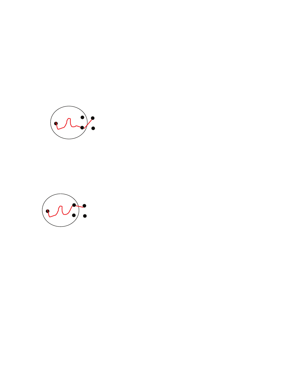
51
Since we need to find a fastest way through S
1,n
, let us be more general and find a structure of a fastest
way through S
1,j
. for 1
≤j≤n [[we shall see that an argument about a fastest way through S
2,j
is symmetric]].
The case when j=1 is easy, so let us consider it first. There is just one route through S
1,1
, and its routing
time is e
1
+a
1,1
, which is trivially the fastest way through S
1,1
.
The case when j≥2 is more interesting. We shall see that the fastest routing time can be achieved by using
a fastest way through “preceding” stations. Pick a station S
1,j
for j
≥2, and a route that yields the fastest
way to get the chassis from the starting point through the assembly lines and complete the processing at
the station. This route is passing either through S
1,j-1
or S
2,j-1
. Let us assume it is S
2,j-1
(
red
) [[the case of
S
1,j-1
in is similar]]. So we can represent the situation as follows:
Let t be the time for the chassis to get from start through S
2,j-1
on the (
red
) route. So the time to get
through S
1,j
on the route is t+t
2,j-1
+a
1,j
. Let t’ be the fastest time to get from the start through S
2,j-1
on a
route. We observe again that t=t’, because if t>t’, then we could use this (alternative) route that gets us
through S
2,j-1
in t’ and then get through S
1,j
in time t’+t
2,j-1
+a
1,j
, which would be strictly quicker than the
way that we assumed is a fastest one. So we can get to S
1,j
in (the fastest) time t using a fastest way to S
2,j-
1
. The following situation
can be argued in a similar way. If a fastest way from the start to S
1,j
passes through S
1,j-1
, then we can get
through S
1,j
in the same time by first getting through S
1,j-1
in the fastest possible time, and then going to
S
1,j
directly [[where the chassis experiences a
1,j
processing time]].
We observe that the argument about the fastest way to get through S
2,j
[[on the second assembly line]] is
symmetric.
We summarize our reasoning about the structure of optimal solution. The fastest way to get through
station S
1,j
is either
the fastest way to get through station S
1,j-1
plus a
1,j
, or
the fastest way to get through station S
2,j-1
plus t
2,j-1
plus a
1,j
.
Note that we do not know if an optimal route arrives at S
1,j
from S
1,j-1
or S
2,j-1
, but it must arrive from one
of them.
start
S
1,j
S
2,j
S
2,j-1
S
1,j-1
start
S
1,j
S
2,j
S
2,j-1
S
1,j-1
t
t
2,j-1

52
Similarly, the fastest way to get from the starting point through station S
2,j
is either
the fastest way to get through station S
1,j-1
plus t
1,j-1
plus a
2,j
, or
the fastest way to get through station S
2,j-1
plus a
2,j
.
Thus an optimal solution contains within itself optimal solutions to subproblems -- this is a very
important observation about the structure of optimal solution that allows to significantly speed up the
computation.
2) A recurrence
The second step of dynamic programming is to write a recurrence for the optimal value, here minimum
routing time. For this purpose, we will use our observations about optimal structure [[later we will deal
with how to find an optimal route that yields this minimum routing time]]. We first define what we want
to calculate and then describe how to calculate this recursively. What we want to calculate is the fastest
time f
i,j
to get from the starting point through station S
i,j
.
For the base case j=1, note that f
1,1
is easy to calculate, because there is just one way to get from the
starting point through station S
1,1
,
f
1,1
= e
1
+a
1,1
.
Similarly
f
2,1
= e
2
+a
2,1
.
Now the key part is to calculate f
1,j
for j at least 2. We focus on f
1,j
first [[we shall see that the case of f
2,j
is
symmetric]]. Let us compare
f
1,j
with
min{ f
1,j-1
+a
1,j
, f
2,j-1
+t
2,j-1
+a
1,j
}, for j
≥2.
Our goal is to conclude that they are equal. Obviously the minimum is ≥ than f
1,j
, because each of the two
numbers inside the curly braces of the minimum corresponds to the routing time of a route through S
1,j
,
while f
1,j
is the minimum routing time through S
1,j
by definition. This was easy. Now the key observation
is that the reverse inequality also holds. Indeed, a fastest way through station S
1,j
leads either through
station S
1,j-1
or S
2,j-1
. When a fastest way leads through S
i,j-1
, then, as we already observed, the chassis
must be through station S
1,j-1
at time f
1,j-1
, and then it will be through S
1,j
at time t
1
:= f
1,j-1
+a
1,j
. However,
when a fastest way leads through S
2,j-1
, then, again as we already observed, the chassis must be through
station S
2,j-1
at time f
2,j-1
and then it will be through S
1,j
at time t
2
:= f
2,j-1
+t
2,j-1
+a
1,j
. So min{t
1
,t
2
} bounds
from below the fastest time through S
1,j
! Since the two inequalities hold, it must be the case that
f
1,j
= min{ f
1,j-1
+a
1,j
, f
2,j-1
+t
2,j-1
+a
1,j
}.
We can use a similar argument to conclude that
f
2,j
= min{ f
2,j-1
+a
2,j
, f
1,j-1
+t
1,j-1
+a
2,j
}.
Again using a similar argument we can conclude that the fastest time f* through the factory is

53
f* = min{f
1,n
+x
1
, f
2,n
+x
2
}.
This completes the description of recurrence for calculating the fastest time through the factory.
3) Computation of minimal value [[routing time]]
The recurrence that we have just derived, enables a simple recursive algorithm for evaluating f
1,n
and f
2,n
.
Unfortunately, this gives an exponential algorithm [[which can be observed by counting the number of
times we need to evaluate f
i,j
in the recursive calls – the number grows by the factor of 2 as j decreases]].
We note that subproblems overlap, so we could just remember prior solutions [[this is called overlapping
subproblems]].
A key observation is that when we calculate f
i,j
, we need values of f
i’,j-1
. So we could calculate f
i,j
starting
from j=1, then j=2, j=3 and so on. We can keep the values of f
i,j
in a table, so that we do not have to
recomputed them. [[there are gaps left on purpose in the subsequent code; we will fill them in soon]]
FastestThroughFactory(e
1
,e
2
,a,t,x
1
,x
2
)
1 f[1,1]
← e
1
+a[1,1]
2 f[2,1]
← e
2
+a[2,1]
3 for
j
← 2 to n
4
if f[1,j-1]+a[1,j] < f[2,j-1]+t[2,j-1]+a[1,j]
5
6
f[1,j] ← f[1,j-1]+a[1,j]
7
else
8
9
f[1,j] ← f[2,j-1]+t[2,j-1]+a[1,j]
10 if f[2,j-1]+a[2,j] < f[1,j-1]+t[1,j-1]+a[2,j]
11
12
f[2,j] ← f[2,j-1]+a[2,j]
13 else
14
15
f[2,j] ← f[1,j-1]+t[1,j-1]+a[2,j]
16 if f[1,n] + x
1
< f[2,n] + x
2
17
18
return f[1,n] + x
1
19 else
20
21
return f[2,n] + x
2
4) Computation of minimal solution [[a route]]
The idea is to remember how we got to the station S
i,j
in a auxiliary table r.
r[i,j] is a pair of numbers that says that a best way to get to S
i,j
is from site S
r[i,j]
. This pair can be easily
determined when we calculate the best routing time through a station [[the red code is the extra code that
is sufficient to add]]; finally r[n+1] is also a pair of numbers that says that a best way to the exit is from
site r[n+1].

54
FastestThroughFactory(e
1
,e
2
,a,t,x
1
,x
2
)
1 f[1,1]
← e
1
+a[1,1]
2 f[2,1]
← e
2
+a[2,1]
3 for
j
← 2 to n
4 if f[1,j-1]+a[1,j] < f[2,j-1]+t[2,j-1]+a[1,j]
5
6
f[1,j] ← f[1,j-1]+a[1,j]
r[1,j] ← (1,j-1)
7 else
8
9
f[1,j] ← f[2,j-1]+t[2,j-1]+a[1,j]
r[1,j] ← (2,j-1)
10 if f[2,j-1]+a[2,j] < f[1,j-1]+t[1,j-1]+a[2,j]
11
12
f[2,j] ← f[2,j-1]+a[2,j]
r[2,j] ← (2,j-1)
13 else
14
15
f[2,j] ← f[1,j-1]+t[1,j-1]+a[2,j]
r[2,j] ← (1,j-1)
16 if f[1,n] + x
1
< f[2,n] + x
2
17
18
r[n+1] ← (1,n)
return f[1,n] + x
1
19 else
20
21
r[n+1] ← (2,n)
return f[2,n] + x
2
, r
Now we can print a best route recursively as follows
RouteTo(i,j)
1 if j≥2 then
2 (i’,j’) ← r[i,j]
3 print (i’,j’)
4 RouteTo(i’,j’)
PrintRoute
1 (i,j)
← r[n+1]
2 print
(i,j)
3 RouteTo(i,j)
Theorem
The algorithm FastestThroughFactory finds in time O(n) a route that minimizes the time of
routing through the factory. The algorithm uses O(n) extra memory.
3.2 Matrix chain multiplication
Today we will start investigating another dynamic programming algorithm which will have a more
sophisticated structure than the one for assembly–line scheduling that we have already studied. The new
algorithm will calculate a fastest way to multiply a chain of matrices. The optimal solution for this
problem will contain optimal solution to two subproblems, and the number of possibilities will not be
constant [[in the assembly-line scheduling we had only one subproblem and there were just two
possibilities]].
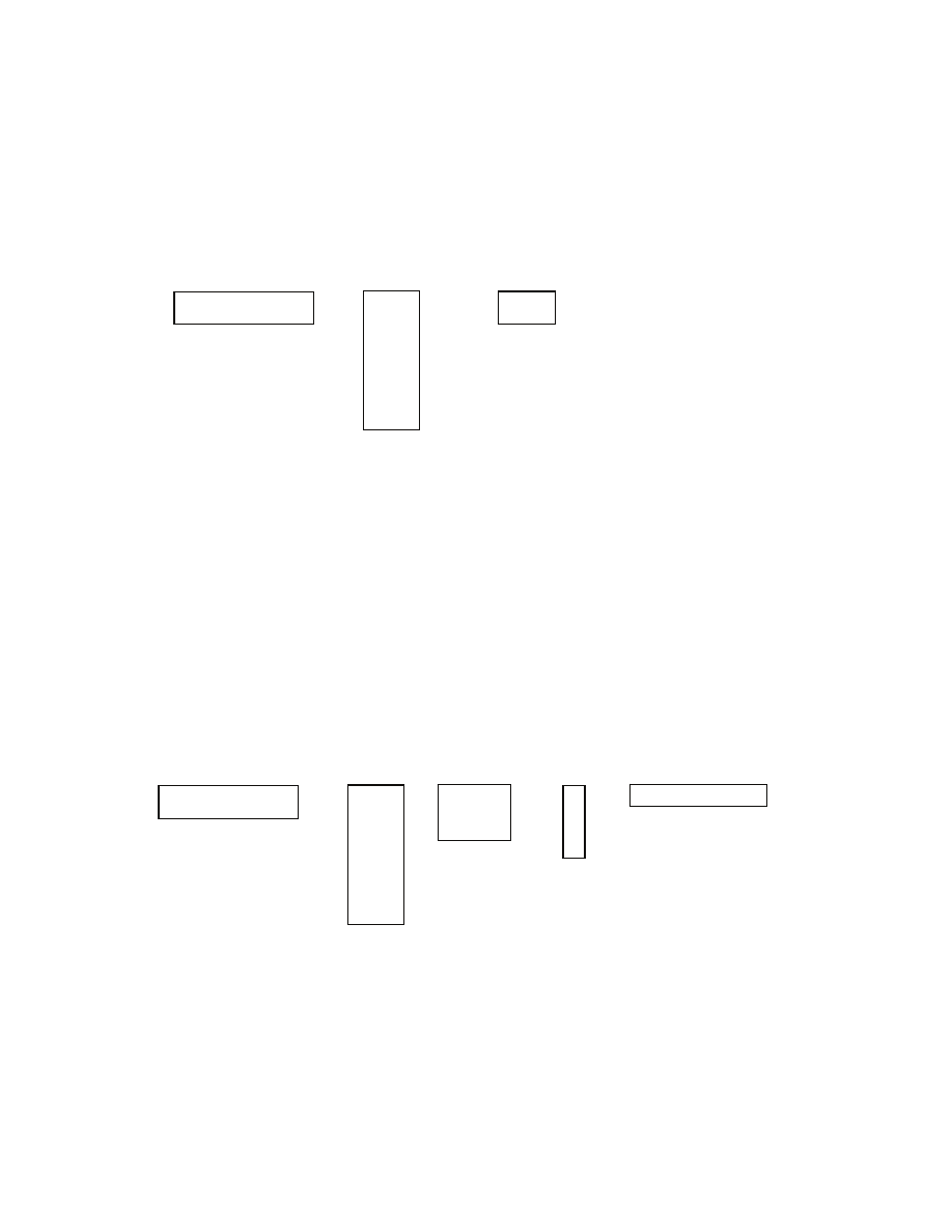
55
Goal: calculate the product A
1
A
2
…A
n
of n matrices as fast as possible.
Background
When is multiplication possible? A
⋅B is possible when matrices are compatible A has p rows q columns,
and B has q rows and r columns. The product has p rows and r columns.
One way to multiply two matrices is to calculate p
⋅r scalar products, each involves q multiplications of
real numbers, and summation [[there are faster algorithms, but let us use this as an example]]; this gives
p
⋅q⋅r multiplications of real numbers [[here we assume that the entries of the matrices are real numbers]].
Then the running time of matrix multiplication is dominated by the number of multiplications of real
numbers; so in the remainder we will assume that the cost of matrix multiplication is the total number of
multiplications of real numbers.
When we need to calculate the product A
1
A
2
…A
n
then the matrices also need to be compatible. We call
this sequence of n matrices a chain, so as to stress the sequence in which matrices need to be multiplied.
It must be the case that A
i
has p
i-1
rows and p
i
columns [[so that the “neighboring” dimensions are equal]],
otherwise the matrices would not be compatible, and so we could not calculate their product.
Multiplication is associative, that is (A
⋅B)⋅C = A⋅(B⋅C) – when A is compatible with B, and B with C. So
we can parenthesize the matrices in various ways. Example of parenthesizing
(((A
1
⋅A
2
)
⋅(A
3
⋅A
4
))
⋅A
5
)
⋅(A
6
⋅A
7
)
p
q
q
r
p
r
A
B
A
⋅B
=
⋅
p
0
p
1
p
1
p
2
A
1
A
2
⋅
A
3
A
4
A
5
p
3
p
4
p
5
p
2
p
3
p
4
⋅
⋅
⋅

56
For a given parenthesization, we may calculate the total number of multiplications of real numbers needed
to calculate the product of the matrices [[we called this total number cost]]. It may be the case that
different parenthesizations may give different costs. Example: suppose that we have three matrices of
dimensions 10
×100, 100×5 and 5×50 – multiplying the later two first “blows up” the size, while
multiplying the former two “collapses” the size [[give numeric values of number of multiplications –
show how total cost is calculated, that is show the sum of individual costs, with dimensions changing;
ONE first 100
×5 and 5×50, which gives 100⋅5⋅50 and a matrix of dimensions 100×50; then 10×100 and
100
×50, which gives 10⋅100⋅50; so the total cost is 25,000+50,000=75,000; TWO gives cost 10⋅100⋅5 +
10
⋅5⋅50 = 5,000+2,500 = 7,500. So costs may be quite different]]
Our goal, thus, is to come up with a way to parenthesize the chain so as to minimize the number of
multiplications [[of real numbers]].
Trivial approach: brute force [[enumerate, and select a lowest]] – the number of choices is at lease 2
n-2
[[here four base cases n=1,2,3,4, for n
≥5 observe that there are at least four summands, and each is a
product that is at least 2
k-2
⋅2
n-k-2
=2
n-4
= 2
n-2
/4 ]], so brute force is not feasible for large n.
Dynamic programming algorithm
We use the pattern of developing DP that we followed for assembly line scheduling.
1) Structure of optimal solution
Lemma
Consider a parenthesization P of A
i
⋅…⋅A
j
for 1
≤i<j≤n that minimizes the cost. Then the last matrix
multiplication in this parenthesization is (A
i
⋅…⋅A
k
)
⋅(A
k+1
⋅…⋅A
j
) for a k that is i
≤k<j i.e., the multiplication
of the product of A
i
⋅…⋅A
k
and the product of A
k+1
⋅…⋅A
j
. Moreover, the same cost is attained by a
parenthesization that parenthesizes A
i
⋅…⋅A
k
in a way that minimizes the cost, and parenthesizes
A
k+1
⋅…⋅A
j
in a way that minimizes the cost, and then multiplies the two resulting matrices.
Proof
We use a “cut and paste” argument, that is if a subproblem was not optimal, then we could replace it with
an optimal one and reduce the cost, which would give contradiction.
Obviously, there is a k as stated in the lemma such that the last multiplication in P is the red dot
(A
i
⋅…⋅A
k
)
•
(A
k+1
⋅…⋅A
j
). Parenthesization P parenthesizes the left subchain A
i
⋅…⋅A
k
somehow, call it L,
and the right subchain A
k+1
⋅…⋅A
j
somehow, call it R. So the last matrix multiplication in P (the
red
dot)
multiplies a matrix that has p
i-1
rows and p
k
columns, with a matrix that has p
k
rows and p
i
columns. So
the cost of this multiplication is p
i-1
p
k
p
j
. Thus the cost of P is the cost of L plus the cost of R plus p
i-1
p
k
p
j
.
Consider a best parenthesization L’ of the left subchain A
i
⋅…⋅A
k
. The cost of L’ is lower or equal to the
cost of L, just because L’ achieves the lowest cost, while L is just the cost of a parenthesization of
A
i
⋅…⋅A
k
. The cost of L’ cannot be strictly lower than the cost of L, because if it were, we could strictly
lower the cost of P, just by replacing the parenthesization L of the left subchain of P with L’ [[here we use
the “additive structure” of cost]]. Similarly, the cost of a best parenthesization R’ of the right subchain
A
k+1
⋅…⋅A
j
is equal to the cost of the parenthesization R. This completes the proof.
█
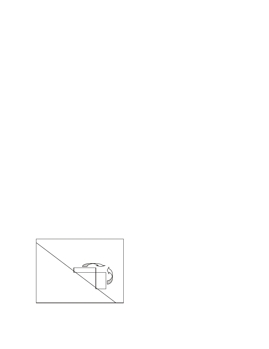
57
2) Recursive equation
The lemma gives rise to the following recurrence. [[again, we define a notion, and then show how to
calculate it recursively]]. Let m[i,j] be the minimum number of multiplications to calculate the product of
A
i
⋅…⋅A
j
for 1
≤i≤j≤n. So the minimum cost is just m[1,n]. The recurrence is
Theorem
m[i,j]=0 when i=j
m[i,j] = min
i
≤k<j
{ m[i,k] + m[k+1,j] + p
i-1
p
k
p
j
}, when i<j
Proof
We consider two cases, organized around the two cases of the recurrence. If j-i=0, the result is trivial
because minimum cost is indeed zero, as stated. Now assume that j-i>0. So the chain has at least two
matrices. We show two inequalities.
First note that the cost min
i
≤k<j
{ m[i,k] + m[k+1,j] + p
i-1
p
k
p
j
} is just a cost of a parenthesization of
A
i
⋅…⋅A
j
. So this cost is at least the minimum cost m[i,j]
m[i,j]
≤ min
i
≤k<j
{ m[i,k] + m[k+1,j] + p
i-1
p
k
p
j
}.
Second, the minimum cost, as explained in the lemma, is attained for a k=k’ and best parenthesizations of
left and right subchains. But then min
i
≤k<j
{ m[i,k] + m[k+1,j] + p
i-1
p
k
p
j
} is at most that minimum cost
because we minimize across all possible k, and so we include k=k’. So
m[i,j]
≥ min
i
≤k<j
{ m[i,k] + m[k+1,j] + p
i-1
p
k
p
j
}
These two inequalities imply that
m[i,j] = min
i
≤k<j
{ m[i,k] + m[k+1,j] + p
i-1
p
k
p
j
}
as desired.
█
3) Algorithm that finds minimum number of multiplications
Key observation is that when calculating m[i,j] we only use shorter chains, so if we calculate m[i,j] for
chains of length 1, then of length 2, and so on, the needed values will already be available. Here is an
picture representing the parts of the table m[] that need to be known in order to calculate the entry m[i,j].
(1,1) (1,n)
(2,2)
(3,3)
(i,i) (i,j)
(j,j)
(n,n)

58
We can implement this order of calculation of entries of m[] as follows.
Parenthesization(p
0
,…,p
n
)
1 for
i
← 1 to n
2 m[i,i] ← 0
3 for
d
← 2 to n
4 for i ← 1 to n-d+1
5 j ← i+d-1
6 best ← ∞
7 for k ← i to j-1
8 if best > m[i,k]+m[k+1,j]+p
i-1
p
k
p
j
9 best ← m[i,k]+m[k+1,j]+p
i-1
p
k
p
j
10
11 m[i,j] ← best
12 return m
4) Algorithm that finds an optimal way to parenthesize
We can compute a best “spit” place k from the table m[] of best costs [[asymptotically same running
time]], but is of often more convenient just to remember the choices in an auxiliary table s[].
Parenthesization(p
0
,…,p
n
)
1 for
i
← 1 to n
2 m[i,i] ← 0
3 for
d
← 2 to n
4 for i ← 1 to n-d+1
5 j ← i+d-1
6 best ← ∞
7 for k ← i to j-1
8 if best > m[i,k]+m[k+1,j]+p
i-1
p
k
p
j
9 best ← m[i,k]+m[k+1,j]+p
i-1
p
k
p
j
10
s[i,j] ← k
11 m[i,j] ← best
12 return m
and s
Now we can print a best parenthesization recursively as follows
PrintPar(i,j)
1 if i=j then
2 print “A
i
”
3 else
4 print “(“
5 PrintPar(i,s[i,j])
6 print “)⋅(“
7 PrintPar(s[i,j]+1,j)
8 print “)“
PrintPar
1 PrintPar(1,n)
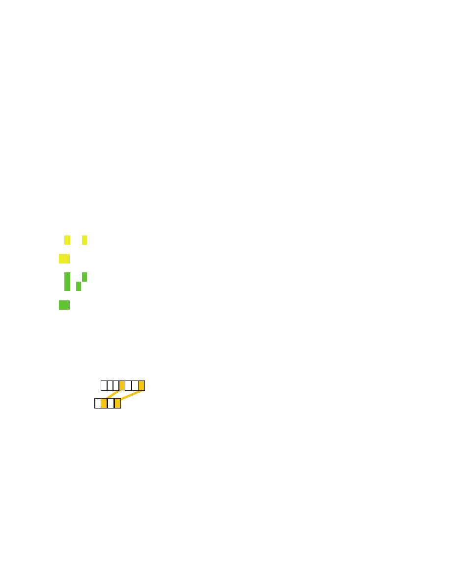
59
Theorem
The algorithm Parenthesization finds in time O(n
3
) a minimum cost parenthesization. The
algorithm uses O(n
2
) extra memory.
3.3 Longest common substring
Today we will see a method that can be used to compare DNA sequences. Suppose that we want to
compare genetic similarities of two organisms. A DNA strand can be represented as a string over the set
{A,C,G,T} e.g., CATGAGAT. Similarity of organisms could be defined as similarity of DNA strands.
We would, however, need to decide what it means for two strings to be similar. We will define one notion
of similarity and give an algorithm for calculating the similarity.
Informally, a string is a sequence of letters, a substring is a string obtained from the string by removing
zero or more letters, and a common substring of two strings is a string that is a substring of each of the
two strings.
Example
string
CAGAT
its substring
AT
two strings
CAGAT
CAATGCC
their common substring
AT
Formally, a string X is a sequence x
1
x
2
x
3
…x
m
, where x
i
is a symbol from a set L of letters, and m≥0 is
called the length of the string. When m=0, then we say that the string is the empty string and denote it by
λ [[lambda]]. A prefix X
r
of the string is the string x
1
x
2
x
3
…x
r
, where 0≤r≤m. A substring of the string a
sequence of indices 1≤i
1
<i
2
<…<i
k
≤m; we can also think of the substring as the sequence x
i1
x
i2
…x
ik
.
Given two strings X=x
1
x
2
x
3
…x
m
and Y=y
1
y
2
y
3
…y
n
, a common substring
is a sequence of pairs of indices (i
1
,j
1
), (i
2
,j
2
), (i
3
,j
3
), …….. , (i
k
,j
k
) such for any pair (i
s
,j
s
) from the
sequence the paired letters are equal x
is
=y
is
and indices are monotonically increasing, 1≤i
1
<i
2
<…<i
k
≤m
and 1≤j
1
<j
2
<…<j
k
≤n; we can think of a common substring as the string x
i1
x
i2
…x
ik
[[for technical reasons
it is convenient to explicitly state which letters get paired up]]; k is called the length of the common
substring.
Longest Common Substring Problem
Input: two strings x
1
x
2
x
3
…x
m
and y
1
y
2
y
3
…y
n
.
Output: their common substring that has the largest length.
X
Y
C
T
T
C
A T G
C G
A
A
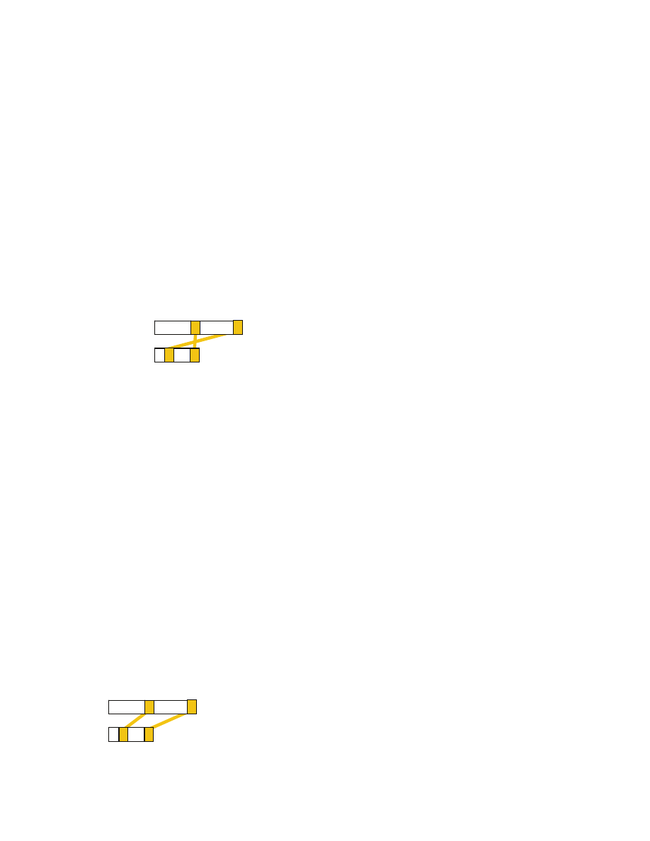
60
1) Optimal structure
[[give intuition for optimal structure – there will be three cases; now the question is how to recognize
which of the three cases holds without knowing S.]]
The comparison between x
i
and y
j
helps us determine whether these letters can be paired in a longest
common substring. The following fact will give rise to three cases.
Fact
Consider any longest common substring S of X
i
and Y
j
. If x
i
≠y
j
, then either no pair in S has the first
coordinate equal to x
i
, or no pair in S has the second coordinate equal to y
j
. If x
i
=y
j
, then there is a longest
common substring of X
i
and Y
j
that contains the pair (x
i
,y
j
).
Proof
Let x
i
be not equal to y
j
. We want to verify that x
i
and y
j
cannot both be paired up (not necessarily in the
same pair). Then of course the pair (x
i
,y
j
) cannot belong to any common substring. A more interesting
case is whether x
i
can be paired with a letter (other than y
j
) and at the same time y
j
can be paired with a
letter (other than x
i
).
But then pairs would “cross” i.e., monotonicity of a sequence of indices would be violated, leading to a
contradiction. Hence either x
i
or y
j
is not paired. [[note that here we do not even use the assumption that
the substring S is a longest common substring]]
Now let x
i
be equal to y
j
. Pick any longest common substring and suppose that it pairs up neither x
i
nor y
j
[[not necessarily to each other; at all]]. Then we could extend the common substring by adding the pair
(x
i
,y
j
) without violating monotonicity. So any common substring must pair up either x
i
or y
j
. Say it is x
i
that is paired up [[the case when it is y
j
will be symmetric]] If it gets paired up with y
j
, we are done as
then pair (x
i
,y
j
) already belongs to longest common substring. So assume that x
i
gets paired up with a
letter y
k
from prefix Y
j-1
. Then we can remove this pair (x
i
,y
k
) and add (x
i
,y
j
) instead, which preserves
length and monotonicity. Thus indeed there exists a longest common substring where x
i
is paired with y
j
.
█
This fact simplifies our analysis of the structure of optimal solution. Just by comparing x
i
with y
j
, we can
determine if (x
i
,y
j
) is in an optimal solution, or if either x
i
or y
j
is not in any pair. Noting these facts, we
pick a longest common substring, look at the last pair, and consider cases depending on how this pair is
arranged within the strings. The cases will be organized around the three cases exposed by the Fact.
Lemma
Consider prefixes X
i
and Y
j
, for 1
≤i≤m and 1≤j≤n, and let S be a longest common substring of the
prefixes. Then a common substring of the same length can be obtained by taking:
1) a longest common substring of X
i-1
and Y
j-1
and appending a pair (x
i
,y
j
), when pair (x
i
,y
j
) is in S,
X
i
Y
j
x
i
y
j
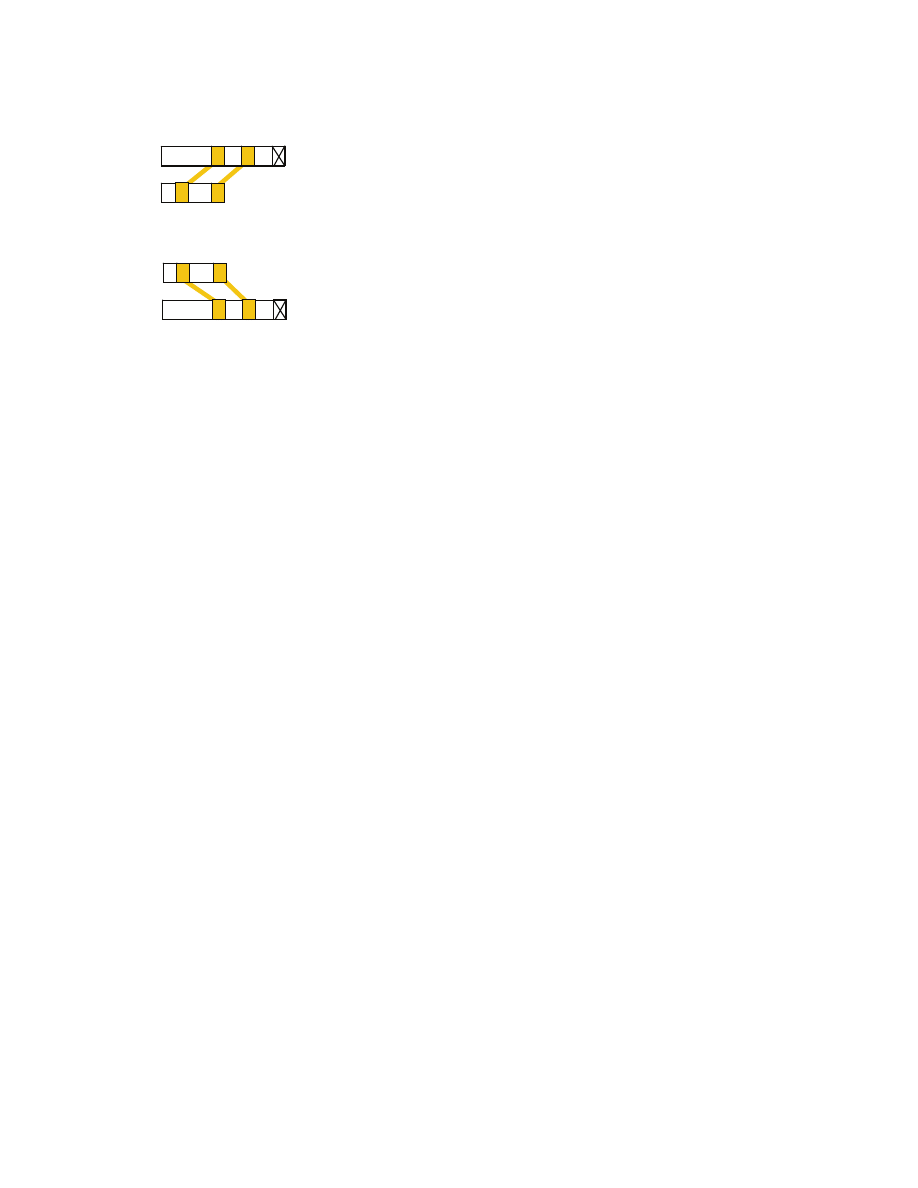
61
2) a longest common substring of X
i-1
and Y
j
, if no pair in S has the first coordinate equal to x
i
,
3) a longest common substring of X
i
and Y
j-1
, if no pair in S has the second coordinate equal to y
j
.
Proof
We consider case 1): x
i
and y
j
are paired by S. Then the common substring S contains a certain number
s
≥1 of pairs. So exactly s-1 of the pairs pair up letters from X
i-1
and Y
j-1
. Pick a longest common substring
S’ of X
i-1
and Y
j-1
. The number of pairs in S’ is at least s-1, because S’ is a longest and there exists one
common substring that has s-1 pairs. S’ cannot have strictly more than s-1 pairs, however, because if so,
we could take S’ and add a pair (x
i
,y
j
), and obtain a common substring of X
i
and Y
j
of length strictly
larger than s, which would contradict the assumption that S is a longest common substring. Therefore, we
can indeed obtain a common substring of length s by taking a longest common substring of X
i-1
and Y
j-1
and appending to it the pair (x
i
,y
j
).
We now consider case 2): x
i
is not paired by S. So S contains a certain number s
≥0 of pairs that pair up
letters from X
i-1
and Y
j
. Pick a longest common substring S’ of X
i-1
and Y
j
. We note that the number of
pairs in S’ must be exactly s. Therefore, we can indeed obtain a common substring of length s by taking a
longest common substring of X
i-1
and Y
j
.
Case 3) is symmetric to case 2).
█
We can combine the Fact and the Lemma, and conclude how to search for a longest common substring.
Corollary
If x
i
=y
j
, then a longest common substring of X
i
and Y
j
can be obtained by taking a longest common
substring of X
i-1
and Y
j-1
and appending a pair (x
i
,y
j
). If x
i
≠y
j
, then a longest common substring of X
i
and
Y
j
is obtained either by taking a longest common substring of X
i-1
and Y
j
or by taking a longest common
substring of X
i
and Y
j-1
, whichever is longer.
2) Recurrence
Let c[i,j] be the maximum length of a common substring of prefixes X
i
and Y
j
, for 0
≤i,j. Of course
c[0,j]=c[i,0]=0, because there is no letter in a prefix of length 0 to be paired with. By the Corollary we
have
{
}
⎪
⎩
⎪
⎨
⎧
=
≥
−
−
+
≠
≥
−
−
=
=
=
j
i
j
i
y
x
and
j
i
j
i
c
y
x
and
j
i
j
i
c
j
i
c
j
or
i
j
i
c
1
,
],
1
,
1
[
1
1
,
,
]
1
,
[
],
,
1
[
max
0
0
,
0
]
,
[
3) Algorithm for max length
X
i
Y
j
X
i
Y
j
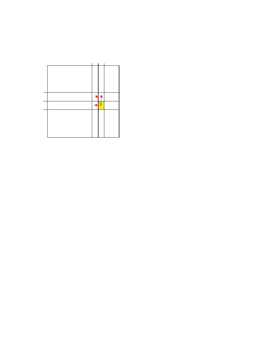
62
We need to observe the sequence in which recurrence could be evaluated so that when we need to
compute c[i,j], then needed entries of the table c[] are already available. Let us depict what c[i,j] depends
on
So we observe that we can fill in c[] row by row, each row from left to right
LCS(m,n,X,Y)
1 for
i
← 0 to m
2 c[i,0] ← 0
3 for
j
← 0 to n
4 c[0,j] ← 0
5 for
i
← 1 to m
6 for j ← 1 to n
7 if x
i
=y
j
then
8 c[i,j] ← 1 + c[i-1,j-1]
9 else
10 if c[i-1,j] > c[i,j-1] then
11 c[i,j] ← c[i-1,j]
12 else
13 c[i,j] ← c[i,j-1]
4) Algorithm for max substring
We can remember how we calculated c[i,j] i.e, if we used the entry to the left, or above, or left-above, in a
table dir[], so that we can later reconstruct a longest common substring.
LCS(m,n,X,Y)
1 for
i
← 0 to m
2 c[i,0] ← 0
3 for
j
← 0 to n
4 c[0,j] ← 0
0 0 0 0 0 0 0 0 0 0
0
0
0
0
0
0
0
i-1
i
j-1 j
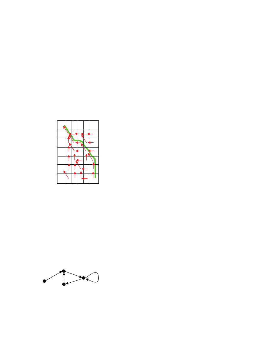
63
5 for
i
← 1 to m
6 for j ← 1 to n
7 if x
i
=y
j
then
8 c[i,j] ← 1 + c[i-1,j-1]
dir[i,j] ← “\”
9 else
10 if c[i-1,j] > c[i,j-1] then
11 c[i,j] ← c[i-1,j]
dir[i,j] ← “|”
12 else
13 c[i,j] ← c[i,j-1]
dir[i,j] ← “-”
Example – how tables are filled in and how to reconstruct a longest common substring.
Theorem
The running time of the LCS algorithm on strings of length m and n is O(m
⋅n); the algorithm used O(m⋅n)
space.
4 Graph algorithms
Definitions
A directed graph is a pair (V,E) where V is a finite set of elements called vertices, and E is a set of
ordered pairs (u,w), called edges (or arcs), of vertices.
A self-loop is an edge (u,u) from a vertex to itself. Ordered pair (u,w) is incident from u and incident to
w; w is adjacent to u [[if there is no edge (w,u) then u is not adjacent to w]]. A path is a sequence
C A
G
A
T
C
A
A
T
G
C
0 0 0 0 0 0
0 1 1 1 1 1
0 1 2 2 2 2
0 1 2 2 3 3
0 1 2 2 3 4
0 1 2 3 3 4
0 1 2 3 3 4

64
(v
0
,v
1
,…,v
k
) of vertices such that there is an edge (v
i-1
,v
i
) for all 1≤i≤k. Then k is the length of the path.
We say that v
k
is reachable from v
0
[[a vertex is always reachable from itself]]. Distance from u to w,
denoted
δ(u,w), is the length of a shortest path from u to w; if there is no path, then distance is defined as
∞.
Representation [[give pictures to exemplify; for directed and undirected]]
• adjacency-list -- an array with n lists, each entry adj[u] has a list of vertices adjacent to u. O(V+E)
space; hard to determine if given (u,w) is an edge of the graph [[scan the list of u]]
• adjacency-matrix -- a
u,w
=1 if there is an edge from u to w, 0 if there is none O(V
2
) space; easy to
determine if (u,w) is an edge of the graph
4.1 Breadth-first search
A graph searching algorithm visits nodes of a graph in a certain order. As a result we can discover some
of graph’s structure. A Breadth-first search (BFS) algorithm traverses vertices in the order of increasing
distance from the starting vertex s, as we shall see shortly.
[[given an example of graph and traversal, the state of the queue Q, tables color[], parent[], and dist[]. and
variables u and w as we iterate through loops; use the word “delta” when speaking about distance, to
distinguish from the table dist[] and avoid verbal confusion]]
Data structures used: Tables: color, dist, parent; FIFO Queue: Q
Nodes will be colored: white [[not yet visited]], visited nodes can be gray [[when its adjacency list has not
yet been traversed]] or black [[when the list has been traversed]]
BFS(G,s)
1 for each vertex v of G
2 color[v] ← WHITE
3 dist[v] ← ∞
4 parent[v] ← NIL
5 Q
← EMPTY
6 color[s]
← GREY
7 Enqueue(Q,s)
8 dist[s]
← 0
9 parent[s]
← NIL
10 while Q is not empty
11 u ← Dequeue(Q)
12 for each w in list adj[u]
13 if color[w] = WHITE
14 color[w] ← GREY
15 Enqueue(Q,w)
16 dist[w] ← dist[u]+1
17 parent[w] ← u
18 color[u] ← BLACK
A node is visited when it is added to the queue in lines 7 or 15. An edge (x,y) is explored when y is
assigned to w in line 12, in the iteration of the while loop when x is assigned to u in line 11.
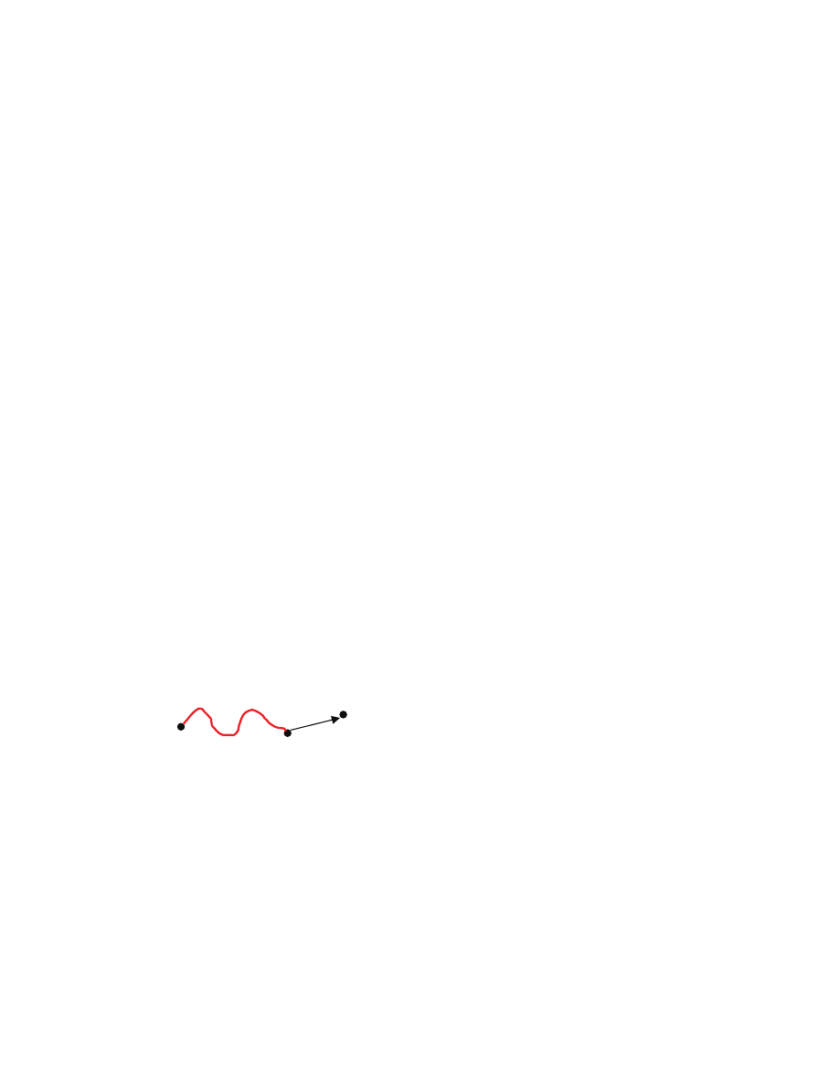
65
[[show an example of execution, how dist[] and color[] get populated, the content of the queue, and how
parent[] get constructed]]
Theorem
The worst-case running time of BFS on a graph G=(V,E) is O(|V|+|E|).
Proof
The loop in lines 1 to 4 runs in O(|V|). Let us count the running time of the loop in lines 10 to 18. We will
do it using a technique of “aggregate accounting”. That loop runs as long as there is a vertex in the queue.
Let us therefore see how many vertices can pass through the queue. By inspecting the code, we notice that
a vertex can be inserted into the queue only if the vertex has just turned from WHITE to GREY (lines
6&7 and 13-15). That vertex later turns BLACK. Thus the vertex never again turns WHITE, and so it can
be inserted into the queue at most once. So the number of times the while loop iterates is at most |V|.
Inside the body, a vertex is dequeued, and its adjacency list traversed. So the time spent inside the body of
the while loop is proportional to the number of edges going out of the vertex. Since each inserted vertex is
dequeued once, the total time [[for all dequeued vertices]] spent on executing the body of the while loop
is O(|E|). This completes to proof of the theorem.
█
We will show that upon termination of BFS, all vertices reachable from s have been visited, for each
vertex v its distance
δ(s,v) from s has been stored in dist[v], and that a shortest path from s to v can be
calculated using the parent[] table. We will do this in a sequence of observations that follow.
Lemma
Consider a directed graph, an arbitrary vertex s, and edge (u,v). Then
δ(s,v)≤ δ(s,u)+1.
Proof
First assume that there is no path from s to u, and so
δ(s,u)=∞, and so δ(s,u)+1 is also infinity [[by
convention 1+
∞=∞]]. But δ(s,v) is either a number [[when there is a path from s to v]], or infinity [[when
there is no path from s to v]]. [[There may be a path from s to v that “goes around u” even though there is
no path from s to u – for directed graphs]]. In either case,
δ(s,v) is at most infinity, and so the upper bound
holds.
Now assume that there is a path from s to u, and so take a shortest path [[as depicted in
red
]] of length
δ(s,u).
But then there is a path from s to v of length
δ(s,u)+1. So a shortest path from s to v can only be shorter or
have the same length. So the upper bound also holds, and so the lemma.
█
BFS computes values dist[u], for all vertices of the graph. We will argue that these values bound from
above distances from s.
u
v
s
δ(s,u)

66
Lemma
When BFS halts, dist[u]
≥δ(s,u), for all vertices u.
Proof
The proof is by induction on the moments when lines 7&8 and 15&16 are executed. The inductive
assumption is that dist[u]
≥δ(s,u), for all vertices u, until the next such moment, or until algorithm halts.
Base case. Lines 7&8 are always executed, and this happens before lines 15&16 are. Right after lines
7&8 have been executed, dist[s]=0, and for all other vertices u, dist[u]=
∞. These of course bound δ(s,u)
from above. By inspecting the code, we notice that lines 7&8 are never executed again. We also notice
that either lines 15&16 are executed, or the algorithm, halts. In any case, entries of table dist[] do not
change until that moment [[either 15&16 or halting, whichever occurs earlier]]. So the inductive
assumption holds.
Inductive step. Suppose that the assumption is true right before line 15 is executed. But then there is an
edge from u to w [[because w is in the adjacency list of u]]. Note that line 16 assigns
dist[w] ← dist[u]+1 .
But by inductive assumption dist[u]
≥ δ(s,u). So right after line 16,
dist[w]
≥ δ(s,u)+1 .
But there is an edge (u,w), so by the previous lemma
δ(s,u)+1 ≥ δ(s,w). Hence
dist[w]
≥ δ(s,w) ,
as desired. So the inductive assumption holds right after lines 15&16 have been executed. Again, either
algorithm executed 15&16 again, or never anymore and halts. In any case we observe that table dist[]
does not change at least until the earlier of the two. This completes the inductive step, and the proof.
█
The next lemma states that the queue holds vertices with monotonically non-decreasing values of dist[]
Lemma
Pick any moment of execution when a vertex u is being dequeued, and let (v
1
,…,v
r
) be vertices in the
queue right before the removal [[r
≥1]]. Then dist[v
1
]
≤ dist[v
2
]
≤ … ≤ dist[v
r
], and dist[v
1
]+1
≥ dist[v
r
] .
Proof
The proof is by induction on the moments when a vertex is being removed [[line 11]].
The base case is to show that the lemma holds right before the first moment when a vertex is removed. But
then the queue consists of just s. So the lemma is definitely satisfied.
The inductive step is to show that, if lemma is satisfied right before vertex u is removed [[line 11]], then it
is also satisfied when at the end of the body of the while loop [[line 18]]. Let v
1
,…,v
r
be the vertices in the
queue right before the removal, r
≥1. Then after removal u is v
1
. There are two cases
Case 1) r=1. So the queue becomes empty after the removal. Then any vertex w added in the for loop has
dist[w]=dist[u]+1, so definitely the lemma holds in line 18.
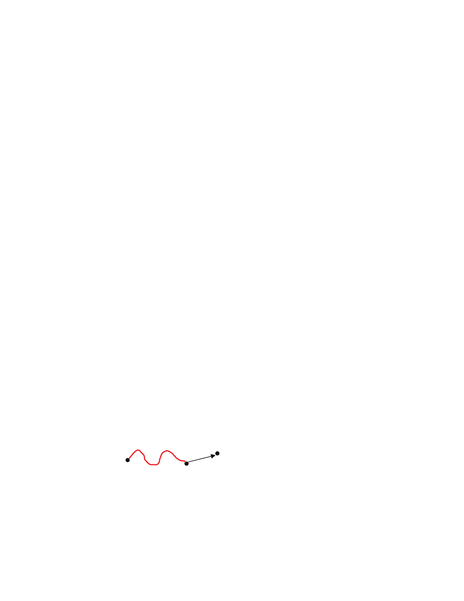
67
Case 2) r
≥2. Recall that dist[v
1
]
≤ dist[v
2
]
≤ … ≤ dist[v
r
], and that dist[v
r
]
≤ dist[v
1
]+1. But any vertex w
added by the for loop has dist[w]=dist[u]+1. Let v
2
,…,v
r
,…,v
m
be the resulting queue [[in line 18]]. So
dist[] for the added vertices are big enough so that the resulting sequence in monotonically non-
decreasing. Now dist[v
1
]
≤ dist[v
2
], and so dist[v
1
]+1
≤ dist[v
2
]+1, and so dist[v
2
]+1 bounds from above
dist[v
m
]. Thus the lemma holds in line 18.
This completes the inductive step, and the proof.
█
Note that for any vertex u, the value dist[u] gets assigned at most once [[the color changes to non-
WHITE, and value can only get assigned when color changes from WHITE to GREY]]. So a vertex can
be inserted into the queue at most once.
Lemma
In any execution of BFS, let u be inserted into the queue before v is. Then, dist[u]
≤dist[v].
Proof
Look at all moments M
1
,M
2
,… when a vertex is about to be removed from the queue [[line 11]]. If
vertices u and v ever reside in the queue at one of these moments, then the lemma follows directly from
the preceding lemma. If vertices never reside in the queue at any such moment, then we reason differently.
We can look at then moment M
u
when u resides in the queue, and M
v
when v resides in the queue. If
vertices in M
i
overlap with vertices from M
i+1
, then we can form a chain of inequalities. If they do not
overlap, then we know that the first vertex added to M
i+1
[[that makes the queue non-empty]] must have
dist[] at least as big as any vertex in the queue M
i
. So we can form a chain anyway. The resulting chain of
inequalities ensures that dist[u]
≤dist[v], as desired.
█
We are now ready to show that BFS correctly computes distances and shortest paths from s.
Theorem
Given a directed graph G and its vertex s, consider the moment when BFS(G,s) has halted. Then for each
vertex v, dist[v]=
δ(s,v).
Proof
The proof is by contradiction. Suppose that there is a vertex v such that dist[v]
≠δ(s,v). This vertex must
be different from s [[ because dist[s]=0=
δ(s,s) ]]. Let us take such v whose δ(s,v) is the smallest; distance
from s is smallest [[break ties arbitrarily]]. So for all vertices w whose distance from s is strictly smaller
than
δ(s,v), dist[w]=δ(s,w). A previously proven lemma states that dist[v]≥δ(s,v), so it must be the case
that dist[v]>
δ(s,v). But the largest dist[v] is infinity, and so δ(s,v) is a number; that means that v is
reachable from s [[because
δ(s,v) is not infinity]]. Take then a shortest path from s to v, and let u be the
vertex right before v on that path.
Our goal is to conclude that dist[u]=
δ(s,u). We can do this if we conclude that δ(s,u)<δ(s,v). But there is a
path from s to u of length
δ(s,v)-1, so δ(s,u)≤δ(s,v)-1. In fact it cannot be the case that δ(s,u)< δ(s,v)-1,
because if there were such shorter way to get from s to u, then there would be a shorter than
δ(s,v) way to
get from s to v. Thus
u
v
s
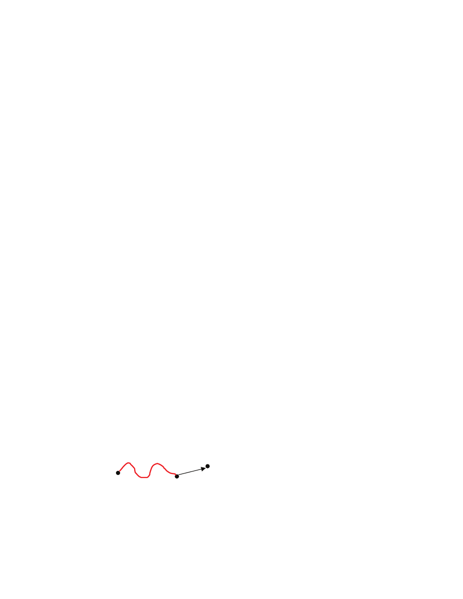
68
δ(s,v) = 1+δ(s,u) .
But then the distance from s to u is one less than the distance from s to v. So the variable dist[u] is, by the
way v was selected, equal to
δ(s,u). Thus
δ(s,v) = 1+δ(s,u) = 1+dist[u] ,
and recalling that dist[v]>
δ(s,v), we have
dist[v] > 1+dist[u].
This is a milestone in the proof. We have concluded that dist[v] must be “significantly” larger than
dist[u], even though there is a direct edge from u to v. Now we shall derive a contradiction by looking at
the moments when vertex u was dequeued and edge (u,v) explored. At the moment of the exploration, v is
either WHITE, or GREY or BLACK. Let us consider these three cases in turn.
Case 1) --- v was WHITE. But then v will get colored GREY (line 14). Then dist[v] will get set to
dist[u]+1, a contradiction.
Case 2) --- v was GREY. Recall that u is not v, and all GREY vertices except for u are in the queue [[u
only becomes BLACK in line 18, while it already is dequeued in line 11]]. Look at the moment when u is
being removed. If v is already in the queue then, by “monotonicity” lemma, dist[v]
≤dist[u]+1, a
contradiction. Can v not be in the queue at the time when u is removed? No, because after removal, we
are adding to the queue (lines 12-17) only vertices adjacent to u, and there is just one edge from u to v.
Case 3) --- v was BLACK. This means that v had been removed from the queue before u was removed.
But vertices are removed in the sequence in which they are inserted. So v occurs earlier than u in the
sequence of vertices inserted into the queue. Here again, by “monotonicity” lemma dist[v]
≤dist[u].
Since we have arrived at a contradiction in each of the three cases, the proof is completed.
█
We now study the structure of “parent pointers” that BFS creates.
Theorem
Let v be reachable from s. When BFS(G,s) has halted, a shortest path from s to v can be obtained by
taking a shortest path from s to parent[v] and then following the edge from parent[v] to v.
Proof
Pick any vertex w reachable from s, other than s. Then 1
≤dist[w]<∞. Consider vertex u=parent[w].
By the way dist[w] is assigned in line 16, we know that dist[w] = dist[u]+1. But then 0
≤dist[u]<∞, and so
a shortest path from s to u has length dist[u], by the previous theorem When can take this path, and added
u
= parent[w]
w
s
dist[u]
dist[w]
= dist[u]+1
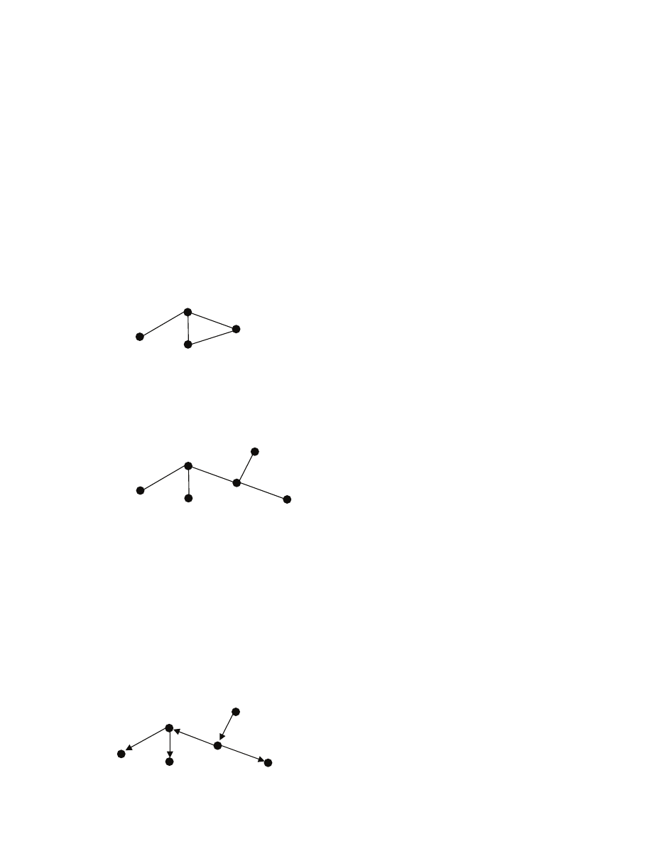
69
to it vertex w. Then we obtain a path from s to w of length dist[u]+1, which is precisely the length of a
shortest path from s to w. Thus the second part is indeed true.
█
Corollary
Pick any vertex v reachable from s. Consider the vertices v
k
,v
k-1
,…,v
0
obtained by following parent
pointers starting from v i.e., v
k
=v, and parent[v
i
]=v
i-1
, v
0
=s [[these do not necessarily need to form a path
in G]]. The reverse sequence v
0
,…,v
k
is a shortest path from s to v.
█
State definition of a tree from B.5.1 and Theorem B.2 from CLRS [[without any proof – done in discrete
mathematics???]]
Definition
An undirected graph, is a pair G=(V,E) such that E is a set of unordered pairs from V, and and self-loops
{w,w} are disallowed.
A path is defined similarity as for directed graphs: a sequence v
0
, …,v
r
r
≥0, of vertices G such that there
is an edge from v
i
to v
i+1
. A graph is connected when for any vertices u and v, there is path from u to v. A
(simple) cycle is a path with r
≥2 such that v
0
=v
r
and v
0
,…,v
r-1
are distinct [[the requirement that r
≥2
ensures that u-v-u --- “go there and back along the same edge” --- is not a cycle]]. A graph is acyclic
when it does not have cycles. A tree is an undirected connected acyclic graph.
Properties of trees [[this is review from discrete math – see section B.5.1 from CLRS]]
Theorem
Given an undirected graph G, the following are equivalent
• G is a tree
• G is connected and |E|=|V|-1
• G is acyclic, and |E|=|V|-1 [[convenient in MST]].
█
A directed graph G is called a tree rooted at a vertex s, when there is a path from s to every vertex in G,
and when the orientation of arcs is ignored, the resulting undirected graph is a tree.
s
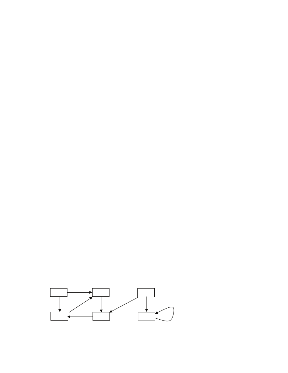
70
Let us invoke BFS(G,s) and upon completion, inspect the content of the table parent. Some vertices v,
will have parent[v] not NIL. When parent[v]
≠NIL, then we interpret this as v points to parent[v], and so
think of the content of the parent table as “parent pointers”. Each parent pointer can be “reversed”, in the
sense that we can consider an edge (v,parent[v]).
Predecessor subgraph G
pred
=(V
pred
, E
pred
) is defined as follows
V
pred
= { v : parent[v]
≠NIL} ∪ {s}
E
pred
= { (parent[v],v) : v
∈V
pred
–{s} }
Theorem
Given a directed graph G, the processor subgraph G
pred
created by BFS(G,s) is a tree rooted at s.
Proof
The proof is by induction on the number of vertices v whose parent[v] is not NIL. We will see that as
BFS(G,s) executes, always the predecessor subgraph is a tree rooted at s.
Initially, all vertices w have parent[w]=NIL. But then G
pred
is a graph with just one vertex s, and edges,
which clearly is a tree rooted at s.
For the inductive step, consider a moment when parent[w] gets assigned u in line 17 of the code. By
inductive assumption G
pred
is a tree rooted at s right before the assignment. The vertex w does not belong
to G
pred
, but u does. So there is a path from s to u in G
pred
and so after we set parent[w]=u, there is a path
from s to w in the resulting G
pred
. The number of vertices of G
pred
increases by one, and so does the
number of arcs. Hence we satisfy the second bullet of the theorem.
█
4.2 Depth-first search
DFS traverses vertices in order such that first it “walks far”, and when it “gets stuck”, it “backtracks”. The
algorithm records the time when each vertex is discovered [[painted GREY]], and when the visit finishes
[[painted BLACK]]
Data structures: tables color[], parent[], disc[] and fin[], and global variable time.
Example [[record discovery time and finish time; record stack of procedure calls; we start at a, and then
we start again at c; vertices in adjacency list are sorted by their letters]]
1/8
2/7
9/12
4/5
3/6
10/11
a
b
c
d
e
f

71
Explain terminology:
We name certain events that occur during an execution of DFS:
• when a function DFS-Visit(u) is first invoked on vertex u, we say that the vertex is discovered;
• when a vertex v is considered in line 11, we say that the edge (u,v) is explored;
• when its adjacency list of a vertex u has been fully examined in lines 11-14, we say that the
vertex is finished.
Coloring scheme: a vertex is initially WHITE; when it is discovered, it is painted GREY; when it is
finished it is painted BLACK.
Timestamps: DFS records time of discovering and finishing vertices. By inspecting the code we see that a
vertex is WHITE until disc[u]-1, GREY from disc[u] to fin[u]-1, and BLACK from fin[u] onwards.
[[Note that time gets incremented when a vertex becomes gray, and when it becomes black, so final time
is 2|V|]]
DFS(G)
1 for each vertex u of G
2 color[u] ← WHITE
3 parent[u] ← NIL
4 time
← 0
5 for each vertex u of G
6 if color[u]=WHITE
7 DFS-Visit(u)
DFS-Visit(u)
8 time
← time+1
9 color[u]
← GREY
10 disc[u] ← time
11 for each v in adj[u]
12 if color[v]=WHITE
13 parent[v] ← u
14 DFS-Visit(v)
15 time ← time+1
16 color[u] ← BLACK
17 fin[u] ← time
Theorem
The worst-case running time of DFS on a graph G=(V,E) is
Θ(|V|+|E|).
Proof
The proof is similar to the proof of running time of BFS. We inspect the code and notice that DFS-
Visit(u) is only invoked when a vertex is WHITE, and then the vertex immediately becomes GREY, and
later BLACK --- it never becomes WHITE again. So the total number of invocations is at most |V|. Note
that it is in fact |V|, because the loop 5-7 invokes the function on vertices that are still WHITE. Inside
each invocation, adjacency list of the vertex is traversed. Since we perform the traversal for every vertex
of the graph, the total time spent in all the loops 11-14, is
Θ(the summation of the lengths of the lists),
which is
Θ(|E|). We perform other instruction in these invocations, which contributes total of Θ(|V|). Thus
the total is
Θ(|V|+|E|), as claimed.
█
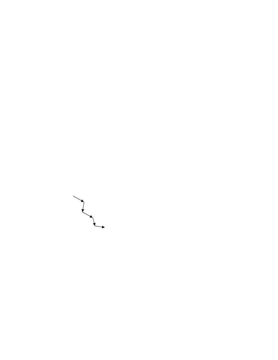
72
We now list several observations about the results produced by DFS.
Similarly to BFS, we can define a predecessor subgraph for DFS as a directed graph G
pred
=(V
pred
, E
pred
) as
follows
V
pred
= V
E
pred
= { (parent[v],v) : v
∈V
pred
such that parent[v]
≠NIL }
This graph is a collection of disjoint rooted trees that combined contain all vertices from V [[formally,
this can be show in a similar way as we did show it for BFS: each invocation of DFS-Visit(u) in line 7
produces a tree rooted at u, that is disjoint with previously produced trees, because the vertices of these
trees are BLACK at the time of the invocation; while the invocation forms links between WHITE vertices
only]]. A graph that is a collection of rooted trees is called a rooted forest. The orientation of arcs in the
directed forest introduce natural orientation of edges; so we can talk about ancestors and descendants [[a
vertex is an ancestor and a descendant of itself, by definition]]. We say that a vertex u is a proper
descendant of v, when u is a descendant of v and u is not v, similarly proper ancestor.
The timestamps assigned by DFS have “nested” structure.
Theorem (Parenthesis theorem)
For any distinct vertices u and v
• if v is a descendant of u in the DFS forest, then disc[u] < disc[v] < fin[v] < fin[u]
• if neither u nor v is a descendant of the other, then the sets {disc[u],…,fin[u]} and
{disc[v],…,fin[v]} are disjoint.
Proof
Suppose that v is a descendant of u. So we have a path u,….,v in the DFS forest [[u and v are different, so
the path has length at least 1]]
Now we will argue about each edge on this path. Recall how an edge in this path is created. An edge (a,b)
is formed when we are inside a call to DFS-Visit(a) and are exploring edges leading out of a. At that time
vertex a is GREY and its disc[a] is already assigned. Then one such edge leads from a to b, and b is
WHITE. Then the edge (a,b) is created and DFS-Visit(b) is invoked recursively. This recursive call
increases current time and sets disc[b] to the time. So disc[a]<disc[b]. The variable fin[a] is only assigned
time, after the recursive call DFS-Visit(b) has returned. But before it returns, fin[b] is assigned. Only then
fin[a] is assigned. So fin[a]>fin[b]. Thus we have {disc[v],…,fin[v]} is included in {disc[u],…,fin[u]}
[[in fact something stronger, as the tips cannot overlap]]. We can follow the path, and make the same
argument for each edge on the path, and thus conclude that disc[u]<disc[v] and that fin[v]<fin[u]. By
inspecting the code we notice that disc[v]<fin[v]. So collecting the inequalities together yields the result.
Now suppose that neither u is a descendant of v, nor v is a descendant of u. Now we have two subcases: u
and v belong to different trees or the same tree. If they belong to different trees, then these trees were
constructed by invoking DFS-Visit in line 7. Then all timestamps recorded during the first invocation are
strictly smaller than any timestamp recorded during the latter invocation. So indeed the sets
v
u
a
b
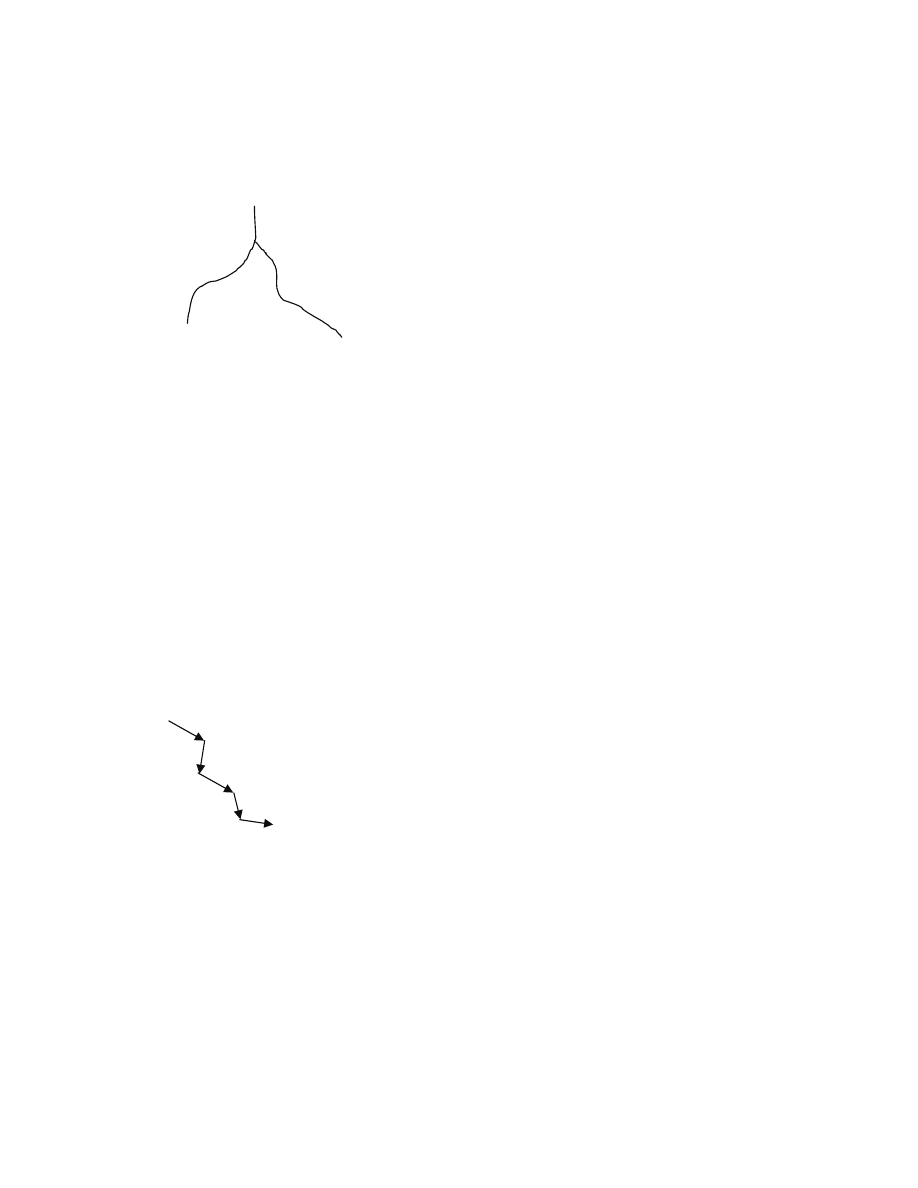
73
{disc[v],…,fin[v]} and {disc[u],…,fin[u]} are disjoint. Say, now that u and v belong to the same tree
rooted at r. Then traverse parent pointers starting from u toward r; we cannot see v on the way. Similarly,
traverse parent pointers starting from v toward r, we cannot see u there. Eventually, these two traversals
must meet at a vertex, call it w [[at the root the latest]].
But then DFS-Visit(w) makes two recursive calls: one on a vertex along the path leading to u, and the
other on a vertex along a path leading to v. All timestamps in the earlier recursive call are strictly smaller
than any timestamp in the later call. So the sets {disc[v],…,fin[v]} and {disc[u],…,fin[u]} are indeed
disjoint.
█
Theorem (White path theorem)
Consider a DFS forest and two distinct vertices u and v. Then the following two are equivalent:
1) v is a descendant of u in the forest
2) at time disc[u] there is a path of length at least 1 in the graph [[not necessarily in the forest]] from
u to v such that all vertices of the path are WHITE except for the first vertex u on the path that is
GREY.
Proof
We show two implications.
“
⇒”
Assume that v is a descendant of u in the forest [[u and v are different]].
The key idea is to use the parenthesis theorem. Consider the moment disc[u]. We want to claim that any
vertex w other than the first vertex on the path is WHITE. But from Parenthesis theorem we know
disc[u]<disc[w]<fin[w]<fin[u]. So vertex w turns GREY after disc[u]. Thus w must still be WHITE at
time disc[u]. So there indeed is a white path from u to v of length at least one.
“
⇐”
Suppose that at time disc[u] there is a path from u to v of length at least one in the graph, and its vertices
are WHITE except for the first vertex u.
u
v
w
v
u
w
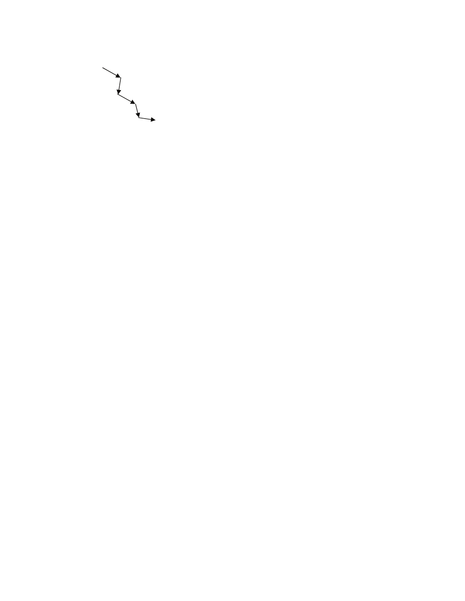
74
Is it possible that v is not a descendant of u in the DFS forest? We will reason about consecutive vertices
on the path, arguing that each must be a descendant of u. Of course u is a descendant of itself. We now
provide the inductive step. Let us pick any vertex p on the path other than the first vertex u, and let q be
the previous vertex on the path [[so it can be that q is u]]. We assume that all vertices along the path from
u to q inclusive are descendants of u. We will argue that p is also a descendant of u.
At time disc[u] vertex p is WHITE [[by assumption about the white path]]. So disc[u]<disc[p]. But there
is an edge from q to p, so q must explore this edge before finishing. At the time when the edge is
explored, p can be:
1) WHITE, then p becomes a descendant of q, and so of u.
2) BLACK, then fin[p]<fin[q] [[because fin[p] must have already been assigned by that time, while
fin[q] will get assigned later]]. But since q is a descendant of u [[not necessarily proper]],
fin[q]
≤fin[u], we have disc[u] < disc[p] < fin[p] < fin[q] ≤ fin[u], and we can use Parenthesis
theorem to conclude that p is a descendant of u.
3) GREY, then p is already discovered, while q is not yet finished, so disc[p]<fin[q]. Since q is a
descendant of u [[not necessarily proper]], by Parenthesis theorem, fin[q]
≤fin[u]. Hence
disc[u]<disc[p]<fin[q]
≤fin[u]. So disc[p] belongs to the set {disc[u],…,fin[u]}, and so we can use
the Parenthesis theorem again to conclude that p must be a descendant of u.
The conclusion thus far is that p is a descendant of u. Now, as long as there is a vertex on the remainder
of the path from p to v, we can repeatedly apply the inductive argument, and finally conclude that the
vertex v is a descendant of u, too.
█
Classification of edges of DFS forest
• tree edges
• back edges --- (u,v) when v is an ancestor of u in DFS forest [[self-loops are back edges]]
• forward edges --- (u,v) is not a tree edge and v is a descendant of u [[self-loops are forward
edges]]
• cross edges --- all other edges; between trees and within a tree but between vertices that are not
one another descendant
v
u
p
q
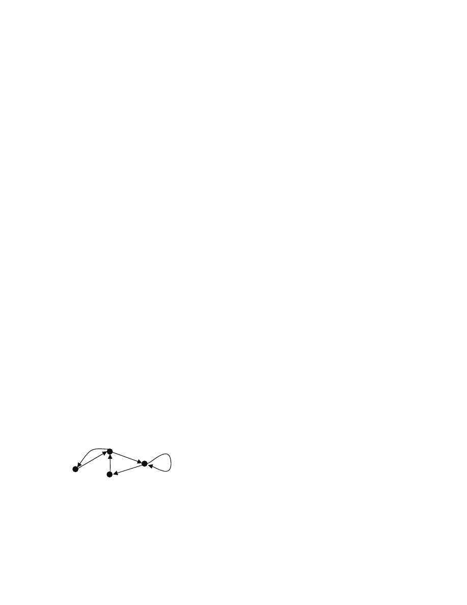
75
Lemma (Back edge lemma)
An edge (u,v) is a back edge if, and only if, when the edge is explored at u, vertex v is GREY.
Proof
“
⇒”
Pick any edge (u,v) that is a back edge. So v is an ancestor of u. By Parenthesis theorem disc[v] < disc[u]
< fin[u] < fin[v]. Consider the moment when the edge (u,v) is explored at u. This must be at a time
between disc[u] and fin[u] inclusive. Hence v is still GREY then.
“
⇐”
Consider the moment when the edge (u,v) is explored at u, and suppose that v is GREY then. Let us
determine which vertices are GREY. A vertex u becomes GREY just after DFS-Visit(u) gets invoked
[[see line 9 of the code]], and stops being GREY when the invocation is about to return [[see line 16 of
the code]]. Consider now the stack of calls at the time when the edge (u,v) is being explored [[line 11 of
the code]]. The stack looks like this:
DFS-Visit(u)
DFS-Visit(u
k
)
…
DFS-Visit(u
2
)
DFS-Visit(u
1
)
DFS(G)
for a certain k
≥0. Hence exactly the vertices u
1
,…,u
k
,u are GREY and any other vertex is either BLACK
or WHITE at that time. Since v is GREY, it must be one of u
1
,…,u
k
,u. By recalling how entries of the
parent table get assigned, we conclude that parent[u
2
]=u
1
, parent[u
3
]=u
2
,…, parent[u
k
]=u
k-1
, parent[u]=u
k
.
Hence the DFS tree has a path u
1
,u
2
,…,u
k
,u. In particular u
1
,…,u
k
,u are ancestors of u in the DFS forest.
Thus v is an ancestor of u, and so edge (u,v) is a back edge.
█
4.3 Topological sort
[[Give a realistic example of events, dependencies between them, and their ordering the events ---
building a home]]
Suppose that you have a certain set of tasks to perform, and there are dependencies between some of these
tasks [[so that a task can be executed only after certain tasks have been executed]]. Today, we will find
out how to sequence the execution of the tasks so as not to violate the dependencies, if possible.
In a directed graph, a cycle is a path of length at least one in which v
0
=v
k
. The definition is different from
the definition of a cycle for undirected graphs, because in the following directed graph
(c,c) is a cycle, so is (a,b,a), so is (b,c,d,b,c,d,b). A directed graph with no cycles is called directed acyclic
graph (dag). Applications – modeling precedence among events / tasks.
a
b
c
d
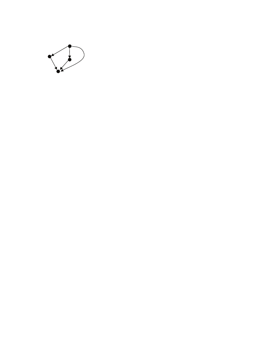
76
Definition
Topological sort is a linear ordering of vertices consistent with the edges of a directed graph i.e., if there
is an edge (u,v) in the graph, then u occurs (strictly) before v in the ordering [[this implies that if there is
an edge (v,v) then v should occur before v -- impossible]]
Given the previous dag, (a,b,c,d) is a topological sort, and so is (a,c,b,d), but not (b,a,c,d).
Main questions:
Given a directed graph, is there a topological sort of the graph?
How to find a topological sort of a given graph?
Lemma
If a directed graph has a cycle, then it does not have a topological sort.
Proof
We reason by way of contradiction. Suppose that we have a directed graph on n vertices with a cycle
v’
0
,…,v’
m
, and the sequence v
1
,…,v
n
is a topological sort of the graph. Then the vertex v’
0
must appear
somewhere in the sort. But since the vertices are on a cycle, there is an edge from v’
0
to v’
1
, and so since
the sequence is a topological sort, v’
1
must appear to the right of v’
0
in the sequence. Repeating this
argument, we obtain that v’
m
must appear to the right of v’
0
in the sequence. But there is an edge from v’
m
to v’
0
and so v’
0
must be to the right of v’
m
, while it actually is to the left. This creates a desired
contradiction and completes the proof.
█
Now, interestingly enough, there is a quick algorithm that finds a topological sort for any directed acyclic
graph. We will study this algorithm in the remainder of the lecture. The algorithm is derived from DFS.
The intuition is that when we run DFS, as we backtrack, the vertices “below” are already finished, so if
we reversely order vertices by finishing times, then we should get topological sort.
Topological-Sort(G)
1 List
← EMPTY
2 run DFS on G with the following modifications
a) when a vertex is being finished, insert the
vertex at the front of List
b) during exploration of any edge (u,v), if v is
GREY exit with a result “graph has a cycle, no
TS exists”
3 print “TS exists”
4 print List from front to end (the reverse order of
insertions)
b
a
c
d
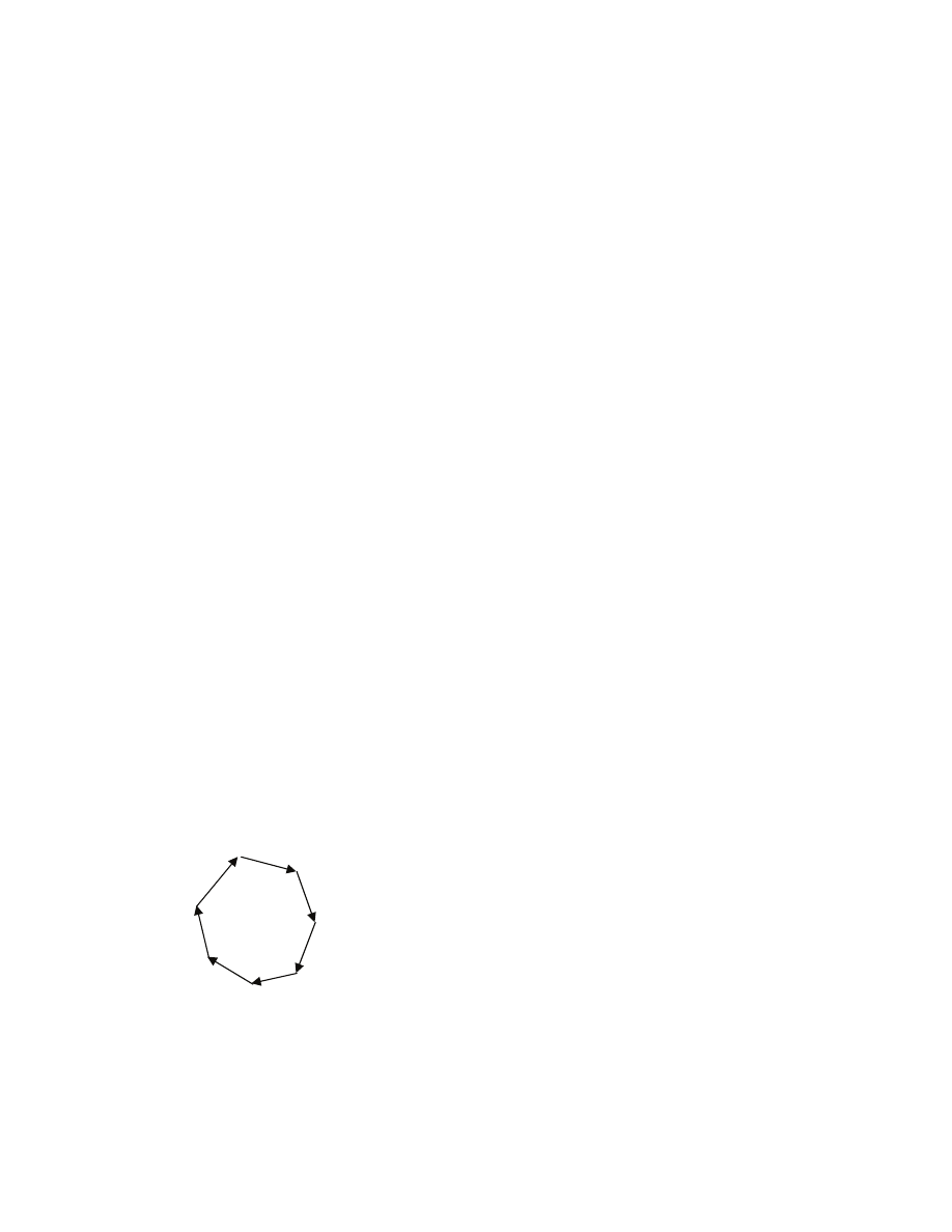
77
An immediate consequence of the theorem on running time of DFS is the following theorem on running
time of Topological-Sort.
Theorem
The worst-case running time of Topological-Sort is
Θ(|V|+|E|).
█
Our next step is to prove that the algorithm is correct. We first observe that we can characterize dags by
lack of back edges. This will demonstrate that the decision made in line 2b is correct.
Lemma
A directed graph has a cycle if, and only if, DFS produces a back edge.
Proof
“
⇐”
Suppose that there is a back edge (u,w). We have two cases:
1) u=w, then this edge is a self-loop, and so a cycle exists in the graph.
2) u
≠w, then w is a proper ancestor of u in the DFS forest, and so there is a path in the DFS forest
from w to u. This path, along with the edge (u,w) form a cycle.
“
⇒”
Suppose that there is a cycle v
0
,…,v
k
, k
≥1. We first modify the cycle so as to ensure that every its vertex
except for the last is distinct.
Removal:
Suppose that vertex u occurs twice among v
0
,…,v
k-1
. Then the sequence looks like this: v
0
,…,v
i-
1
,u,
v
i+1
,…,v
j-1
,u,
v
j+1
,…,v
k-1
. But then we can remove the red part and obtain a path v
0
,…,v
i-1
,u,v
j+1
,…,v
k-1
.
Notice that a duplicate u is gone, and that we never remove v
0
.
We can apply the removal as long as a vertex occurs twice, and as a result obtain a cycle C’ = v’
0
,…,v’
k’
such that vertices v’
0
,…,v’
k’-1
are distinct.
The remainder of the proof is organized around two cases:
1) k’=1, but then the cycle C’ is a self-loop, and so a back edge
2) k’
≥2, then pick the vertex v of the cycle C’ that is first discovered by DFS. So there is an edge
(u,v) in the cycle, and u is not v.
At the time of discovery of v, v is GREY and all other vertices of the cycle C’ are WHITE, so there is a
white path from v to u. By the White path theorem, u becomes a descendant of v in the DFS forest. But
then the edge (u,v) is an edge from a vertex to an ancestor – thus a back edge.
█
v (GREY)
u
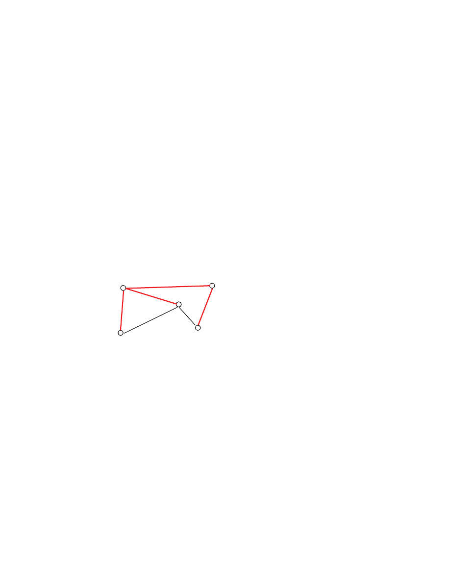
78
Theorem
If graph G is a dag, then TS produces a topological sort of the graph.
Proof
What we need to show that if there is an edge (u,v), then v is finished earlier than u, fin[u]>fin[v].
Consider the moment when the edge is explored. Then the color of u is GREY. What is the color of v?
Can v be GREY? No, because if so then by the Back Edge lemma (u,v) would be a back edge, and then
by the previous lemma there would be a cycle in G, while we know that G is acyclic. So the color of v is
either WHITE or BLACK. When WHITE, then by the White Path theorem v becomes a descendant of u,
and so by the parenthesis theorem fin[v]<fin[u], as desired. When BLACK, then fin[v] has already been
assigned, while fin[u] has not yet been assigned. So again fin[v]<fin[u].
█
4.4 Minimum Spanning Tree
Consider the following transportation problem. We are given n cities, and the costs of constructing a road
between pairs of cities [[for some pair we may not know the cost of building a direct road, or the cost may
be just too high to even consider building a road between them]]. We want to build roads so that we can
drive from any city to any city [[possibly indirectly by passing through some intermediate cities]], and the
total cost of the road construction is minimized. We can model this setting as a connected undirected
graph where edges have positive weights [[if the graph is not connected, then in the corresponding “real
world” problem we obviously cannot build roads so that you can drive between any two cities!]].
We now want to select a subset of edges of the graph such that any two vertices of the graph are
connected by a path from the subset (such as the subset of
red
edges in the picture) and the total weight of
the selected edges is minimized. Such subset has a specific structure. If we pick any subset in which every
two vertices are connected by a path and some selected edges form a cycle [[such as when we were to add
edge with weight 9]], then we could remove an edge of the cycle and strictly decrease the total weight,
while preserving connectivity [[every two vertices of the graph will still be connected by a path of
selected edges]]. But such a set of selected edges is a tree by definition; moreover it contains |V| vertices,
thus is a tree that “spans” all vertices of the graph.
Definition
Given an undirected graph G=(V,E), a spanning tree is a subset of |V|-1 edges of G that form no cycles.
Formally, the optimization problem is defined as follows. We will use the notation u-w to represent an
edge between u and v, so as to stress that the edge has no direction.
Minimum Spanning Tree Problem (MST)
Input: An undirected connected graph G=(V,E), and a weight function w that assigns an integer weight
w(u-v) to each edge u-v of the graph.
10
5
3
4
2
9

79
Output: A spanning tree T of G that minimizes the total weight.
[[notice that if we allow weights to be negative, then our “real life” problem may not require that the
subgraph be a tree, as removal of edges may actually increase the total weight – in the extreme case when
all edges have negative costs, then it is best to select every edge! However, we will allow the weights to
be negative for the purpose of generality, while require that the selected edges form a spanning tree to
model the “real life” problem where weights will be positive]]
Our goal is to develop an efficient algorithm that solves the problem. The algorithm that we will present
will use a “greedy” strategy – it will keep on selecting edges that are “locally” optimal, and these locally
optimal decisions will turn out to eventually give a globally optimal solution. Greediness is an important
technique for designing algorithms for optimization problems -- it does not always work, though
[[however, it very often gives a solution that is close to an optimal one; sometimes we can be satisfied
with “good” but not necessarily optimal solution]].
Structure of a Minimum Spanning Tree
The idea of the algorithm is to take a set that is a part of a minimum spanning tree and decide how to
“extend” the set by adding an edge. We define a notion of a “safe edge” that is useful when extending the
set. Consider a set A of edges, A
⊆E, such that A is a subset of a minimum spanning tree T [[set A may
already be a minimum spanning tree]]. An edge u-v from E that does not belong to A is called a safe edge
for A, if the set A extended by the edge, A
∪{u-v}, is a subset of a minimum spanning tree T’ [[the two
trees T and T’ may be different, the edge u-v does not have to share an endpoint with any edge already in
A, but may share]]
[[the upper edge with weight 2 that is in T, can be replaced with the lower edge with weight 2, and we
still get a minimum spanning tree, so the edge does not have to belong to the tree T, it may belong to a
different T’]]
The central question that we need to answer is how to find a safe edge. We postponed answering the
question for some time. Indeed, suppose for a moment that we know how to find a safe edge for A, if such
an edge exists. With this assumption, we can build a minimum spanning tree as follows.
Generic-MST(G)
1 A
← EMPTY
2 while |A| < |V|-1
3 u-v ← safe edge for A
4 A ← A∪{u-v}
Why is this algorithm correct? Observe that there always is a minimum spanning tree for a connected G.
So after we have initialized A to an empty set, we can claim that A is a subset of a minimum spanning
A
⊆
T
9
1
1
1
1
safe
edge
1
1
2
2
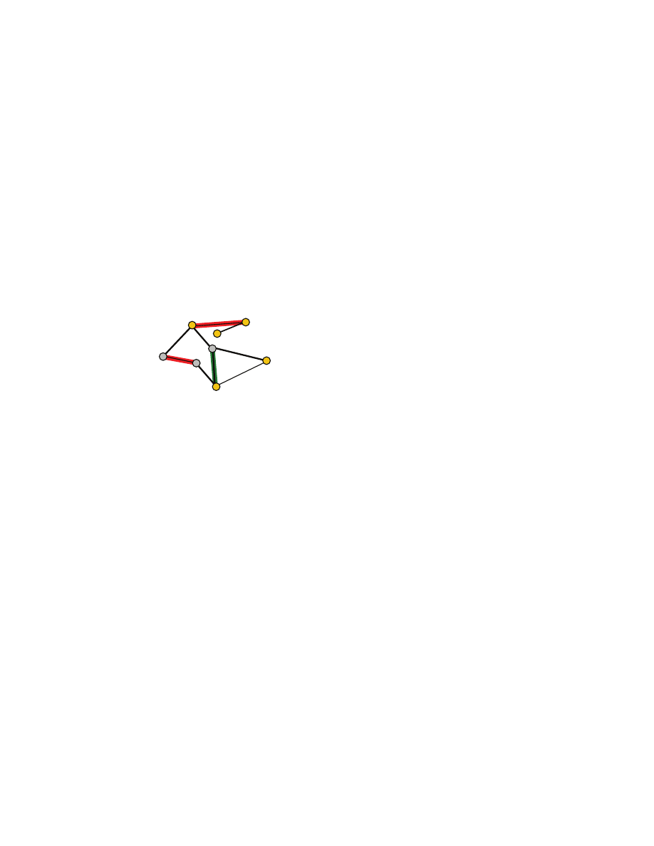
80
tree. We shall maintain this claim as a loop invariant. Right before line 3 is executed, set A is a subset of a
minimum spanning tree T, and has cardinality at most |V|-2. Since T is a spanning tree, T has |V|-1 edges.
So there is a tree edge that does not belong to A. So there is a safe edge. So we can select a safe edge in
line 3 [[there may be many safe edges, we select one]]. Let u-v be this safe edge and let T’ be the
minimum spanning tree such that A
∪{u-v}, is a subset of T’. After we have added the edge to A, the
resulting set A has the property that it is contained in a minimum spanning tree. So loop invariant holds
again. Finally, when the loop terminates the cardinality of A is |V|-1, and A is a subset of a minimum
spanning tree T’’. But the tree has |V|-1 edges, so A=T’’, and so A is indeed a minimum spanning tree.
The preceding argument motivates why the notion of a safe edge is useful. So what remains to be done is
to decide how to select a safe edge for A, when A is a subset of a minimum spanning tree. It turns out that
we can select a specific edge that has the lowest weight. This is explained in the following lemma. Before
we state and prove the lemma, let us introduce a few notions.
Given a connected undirected graph G=(V,E) a cut is a partition (C,V-C) of the vertices of the graph such
that neither C nor V-C is empty [[so C may comprise “disconnected” parts, see
gold
and
grey
in the
figure]].
Given a subset A of edges, we say that the cut respects the subset if “edges do not cross the cut” that is
each edge from A has both endpoints in C or both endpoints in V-C [[
red
in the figure]]. Given a cut, we
can look at all edges “crossing the cut” i.e., with one endpoint in C and the other in V-C [[bold black in
the figure]] [[since G is connected, and C nor V\C is empty, there is always an edge that crosses the cut]].
The crossing edges may have different weights. Any of these edges that has the smallest weight is called a
light edge of the cut [[
green
in the figure]].
[[picture that exemplifies the definitions]]
Lemma (Safe edge lemma)
Let A be a subset of edges that belong to a minimum spanning tree T of G=(V,E). Let (C,V-C) be a cut of
G that respects A. Let u-v be a light edge of the cut. Then the edge is a safe edge for A.
Proof
Let us consider two cases: u-v belongs to T, and u-v does not belong to T. Notice that u-v does not belong
to A because u-v crosses the cut, while the cut respects A.
1) Edge u-v belongs to T. But then A
∪{u-v} is obviously included in T. But since u-v does not belong to
A, the edge u-v is a safe edge.
2) Edge u-v does not belong to T. Since T is a spanning tree, there is a path of edges of T connecting u
and v [[
green
]]. That path cannot contain u-v.
1
2
A
9
1
1
1
1
1
2
C
,
V\C

81
Since u and v are on the opposite sides of the cut, there must be an edge x-y of the path that crosses the
cut [[and of course the edge x-y is different from the edge u-v]]. But then that path along with the edge u-
v form a cycle. We can remove edge x-y from T and add edge u-v instead, and the resulting subgraph is
still a spanning tree [[it has |V|-1 edges and any two nodes are connected – simply because if a connecting
path includes x-y, then we can remove that edge and replace it by the path that goes around through u-v]].
How about the weight of the resulting spanning tree? Edges x-y and u-v both cross the cut, and u-v is a
light edge by assumption, so its weight is at most the weight of the edge x-y. So the resulting tree has
weight at most the weight of T---so minimum weight. But then the set A expanded by u-v is contained in
a minimum spanning tree, and so the edge u-v is again a safe edge.
The proof is thus completed.
█
The lemma suggests how to find safe edges. Say that we have a set A that is a tree with at least one edge,
but not yet a spanning tree. Now we need to find a cut (C,V\C) that respects A. Once we have found the
cut, we can easily find a light edge e, and the lemma promisses that that edge e is a safe edge. Let A’ be
A
∪{e}. Notice that A’ is also a tree, since A’ is definitely connected and we added one new edge e and
one new node, so the number of edges in A’ is one fewer than the nubmer of nodes in A’. One natural
candidate for C is the set of all endpoints of A. Such set will have exactly |A|+1 nodes [[because A forms
a tree]]. After adding e to A, we can repeat the process of finding a safe edge, until A becomes a spanning
tree.
The problem is that we must start off with A that contains at least one edge. Indeed if A is empty, then the
set of all endpoints C is also empty, and so (C,V\C) is not a cut [[because cut must have nonempty C and
V-C]]. So the beginning of our algorithm is not yet determined. However, there is a way to find an edge
that is a safe edge for an empty set.
Lemma (Lightest edge lemma)
An edge with the lowest weight is a safe edge for an empty set.
Proof
The proof is quite similar to the proof of the Safe edge lemma. We need to demonstrate that there is a
minimum spanning tree that contains an edge with the lowest weight. Let u-v be this edge. Pick any
minimum spanning tree T. If the edge is in T, we are done. So assume that the edge is not in T. But then
when we add u-v to T, we get a cycle. Pick any edge on the cycle other then u-v and remove the edge.
The weight of the resulting subgraph is smaller or equal to the weight of T. Moreover, the graph is a tree
since it is connected [[by the same path replacement argument as in the earlier lemma]] and has |V|-1
edges.
█
u
v
x
y

82
4.4.1 Prim’s algorithm
Now we can specialize the Generic-MST algorithm. The first safe edge that we add to A will be a lightest
edge in the graph. Let the set C be the set of all vertices that are endpoints of edges from A. So now the
set contains two vertices. In general, we will maintain an invariant that |C| = |A|+1. Obviously when
|A|<|V|-1, then the C defined like this gives a cut that respects A. We can, therefore, pick a minimum
weight edge that has only one endpoint in C. We then add the edge to A. Thus the resulting A has one
more edge, and the resulting C has one more vertex. We can continue like this until |A|=|V|-1.
Prim’s-MST(G)
1 for each vertex v
2 color[v] ← WHITE
3 find edge u-v with minimum weight
4 A
← { u-v }
5 color[u]
← color[v] ← BLACK
6 heap
← EMPTY
7 for each x in adj[u]
8 Insert(heap, w( u-x ), u-x )
9 for each x in adj[v]
10 Insert(heap, w( v-x ), v-x )
11 while |A|<|V|-1
12 u-v ← RemoveMin(heap)
13 if color[u]=WHITE and color[v]=BLACK
14 A ← A∪{ u-v }
15 color[u] ← BLACK
16 for each x in adj[u]
17 Insert(heap, w( u-x ), u-x )
18 if color[u]=BLACK and color[v]=WHITE
19 A ← A∪{ u-v }
20 color[v] ← BLACK
21 for each x in adj[v]
22 Insert(heap, w( v-x ), v-x )
Theorem
The Prim’s-MST algorithm finds a minimum spanning tree of an undirected and connected graph in time
O(|E|log|E|).
Proof
One can see that the following invariant in maintained by the while loop
(1) any endpoint of an edge from A is BLACK, and no other vertices are BLACK,
(2) heap contains edges each of which has at least one BLACK endpoint,
(3) all edges that cross the cut are in the heap.
This invariant ensures that only a safe edge can be added to A in line 14 and 19.
█
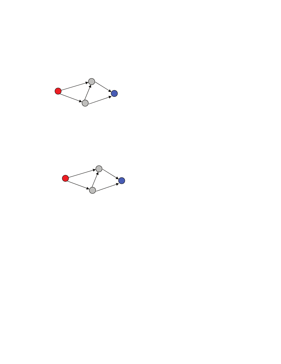
83
4.5 Network Flow
Consider the following problem that can occur when transporting goods. We have a collection of cities,
we can transport goods from certain cities to certain other cities using roads. Each road has a direction. It
also has a
capacity
that states how much goods per second we can transport along the road.
One of the cities is designated as the
source
--- i.e., a base from which the goods will be sent out, and
other city is designated as the
sink
i.e., the target where the goods must be delivered. We want to find out
how much goods we should be sending out of the source along the roads into the sink to maximize the
flow per second out of the source into the sink, while maintaining the capacity constraints. We can only
produce goods at the source, and we can only accumulate goods at the sink.
Consider for example the following
amount
of goods flowing along the roads
Here the flow from s to b is 5, while the flow from s to a is 0. The total flow out of s is 5, and the total
flow into t is also 5=3+2. The flow “forks” at b: flows in as 5 and flows out into two parts: as 3 and as 2.
The amount of flow assigned to each road must satisfy extra properties. Pick any city other than the
source or the sink. If less goods flow in but more flow out, then the city would have to create extra supply
somehow to satisfy the excessive outflow. If less goods flow out but more flow in, then the city would
accumulate the goods. We do not allow for creating not accumulating goods at the cities other than source
and sink. So we require that the amount of goods flowing out must be equal to the amount of goods
flowing in. Moreover, goods should only flow out of the source (but not in), and only flow into the sink
(but not out).
Formal problem statement
Let us now state the problem in abstract terms. We are given a directed graph G=(V,E) without self-loops
[[other cycles are permitted]] with designated node s, called the source, and designated node t, called the
sink, any other node is called internal. For any internal node u, there is a path from s through u to t.
Source only has outgoing edges, and sink only has incoming edges, Each edge e=(u,v) has a capacity c
e
>0
that is a real number [[we will later sometimes assume that each capacity is an integer, but the general
problem statement allows for real numbers]]. Such graph G with capacities is called flow network. A flow
is a function f:EÆR denoting the amount of flow f(e) on edge e. Flow f must satisfy the following
conditions:
s
b
a
t
2
6
8
6
2
s
b
a
t
0
≤
2
3
≤
6
3
≤
8
5
≤
6
2
≤
2
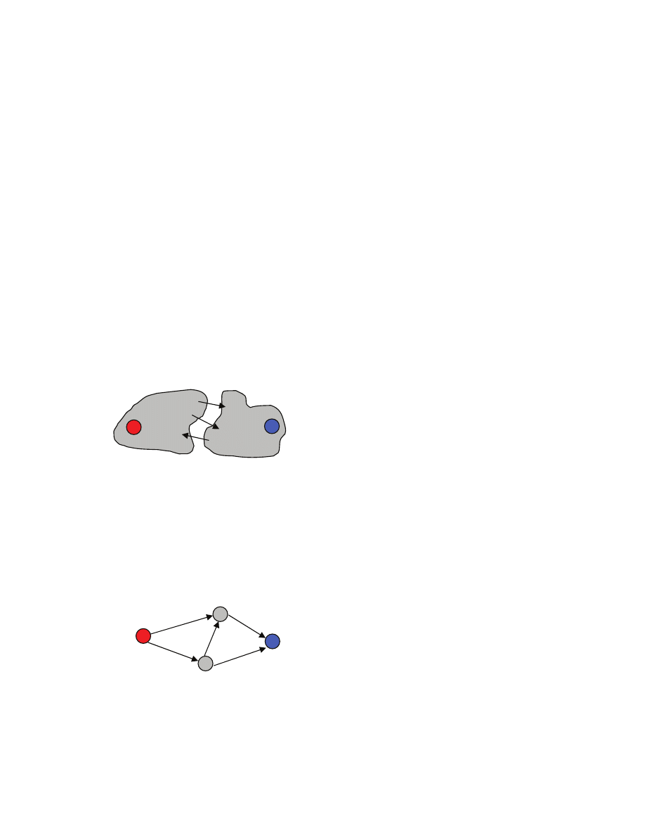
84
1) (capacity) For each edge e, the flow along the edge obeys capacity constraints 0
≤f(e)≤c
e
.
2) (conservation) For each internal node u, the total amount of flow entering u equals the total
amount of flow leaving u
∑
∑
=
u
e
u
e
e
f
e
f
of
out
into
)
(
)
(
The value v(f) of a flow f is defined as the total flow leaving the source
∑
=
s
of
out
)
(
)
(
e
e
f
f
v
. The goal is to find
a flow that has maximum value. We call this problem the Maximum Flow problem (Max-flow)
Theorem
The Max-Flow problem always has a solution.
Proof
Remove for a moment the flow conservation constraint. Think about flow f as a vector (f(e
1
),…,f(e
|E|
)).
That vector can be selected from a domain D=[0,c
1
]
×…×[0,c
|E|
] that is a closed subset of R
|E|
. The value
v(f) is a continuous function of f. Since D is closed and v is continuous, v achieves the maximum for
some f
*
in D [[a standard fact from real analysis]]. Any continuous function is also continuous on any
subset of the domain. The flow conservation requirement constrains the values of f through equations,
each specifying a linear hyperspace of R
|E|
. So the intersection of all these |V| subspaces [[i.e., finitely
many]] with D is also closed. Hence v achieves the maximum value under the capacity and conservation
constraints, as desired.
█
What limits that value of a flow? The intuition is that if you partition nodes into sets A and B such that
source is in A and sink is in B,
then any flow f must at some point cross the boundaries between A and B, and so the flow value is
limited by the capacity of edges leading from A to B, here 8=6+2 [[but not from B to A]]. Hence the
intuition is that the value of the flow is at most the “capacity” of any such partition.
4.5.1 Ford-Fulkerson Algorithm
[[why greedy fails, and the emergence of augmenting path and augmentation]]
We will try to design an algorithm. Let us start with an example flow problem
and suppose that we “push” the flow from the source to the sink greedily selecting the next edge with
largest capacity. Then we will first push 6 units of flow from s to b, and then these 6 units further to a,
and then further to t. The resulting flow is:
s
t
6
2
3
s
b
a
t
≤
2
≤
6
≤
8
≤
6
≤
2
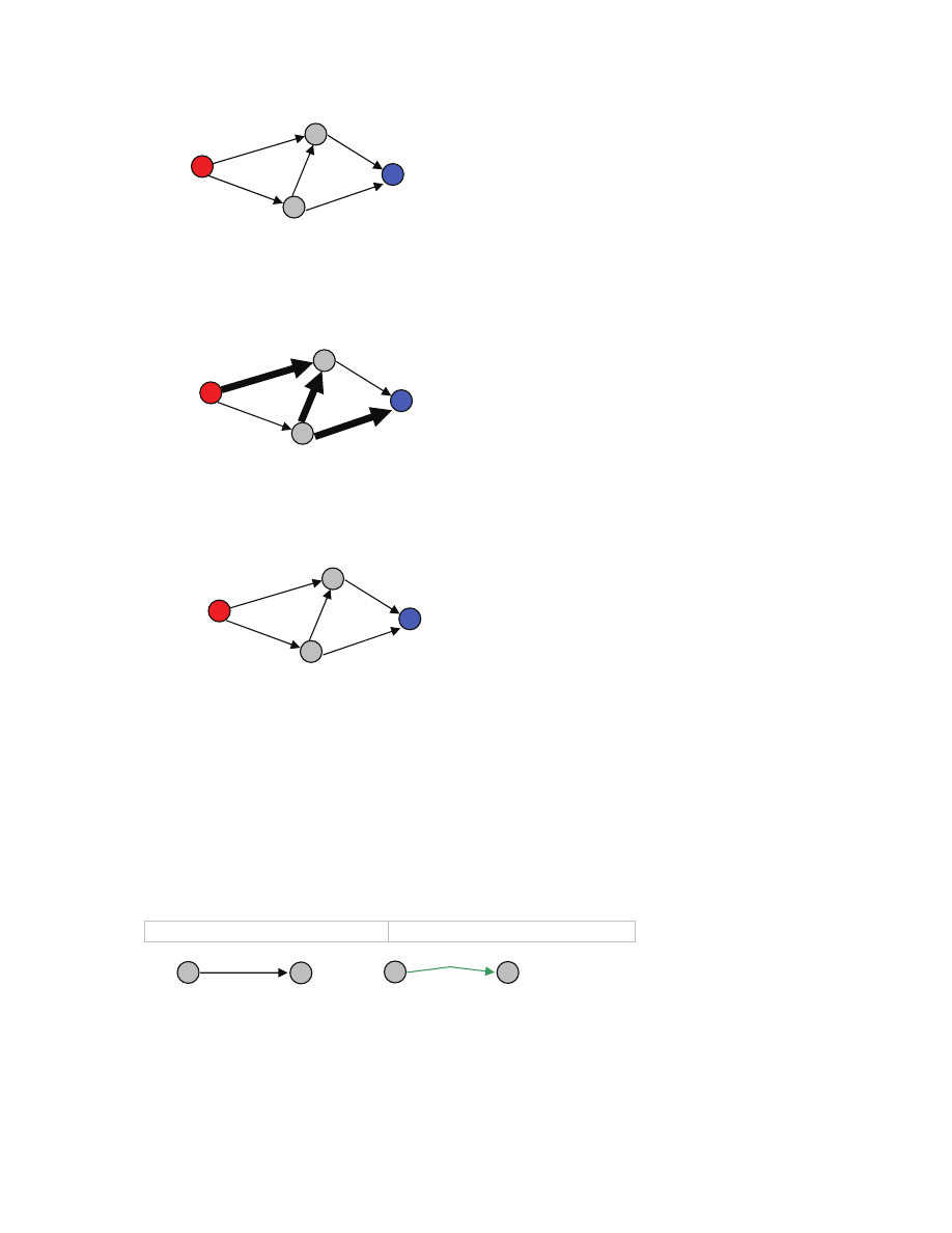
85
At this time we can push no more flow out of s, because the edge from a to t is saturated (carries as much
flow as the capacity of the edge) thus blocking a potential path s,a,t. So the value of this flow is 6. Is this
the maximum? It is not! Let us see how we can modify the flow to increase its value while preserving
capacity and conservation constraints.
We can push 2 units from s to a, thus creating an overflow at a, then unpush 2 units of the flow that
currently flows from b to a to get rid of the overflow at a, thus creating an overflow at b, and finally push
2 units from b to t, thus getting rid of the overflow at b. As a result we get the following flow
which is maximum [[as it saturates every edge leaving the source]].
[[residual graph]]
Let us formalize the idea of modifying a flow. Given a flow network G=(V,E) with capacities and its flow
f, we will build another graph G
f
that represents our ability to modify the flow. The graph G
f
will have the
same set of nodes as G. Every its edge will be labeled with number called a residual capacity.
Specifically the edges and residual capacities are constructed as follows. For any edge e=(u,v) of G
• if f(e)<c
e
, then the current flow does not exhaust the capacity of the edge, and so we could push
more flow in G along the edge. Specifically, we add an edge e=(u,v) to G
f
with residual capacity
c
e
-f(e).
in G with flow f
in G
f
we call the edge added to G
f
a forward edge.
• if f(e)>0, then we have a non-zero flow along the edge, and so there is a possibility to unpush
flow currently flowing along the edge e=(u,v). Specifically, we create a reversed edge e’=(v,u)
with residual capacity f(e)
s
b
a
t
0
≤
2
6
≤
6
6
≤
8
6
≤
6
0
≤
2
s
b
a
t
0
≤
2
6
≤
6
6
≤
8
6
≤
6
0
≤
2
+2
-2
+2
s
b
a
t
2
≤
2
6
≤
6
4
≤
8
6
≤
6
2
≤
2
u
v
2
≤
6
u
v
4
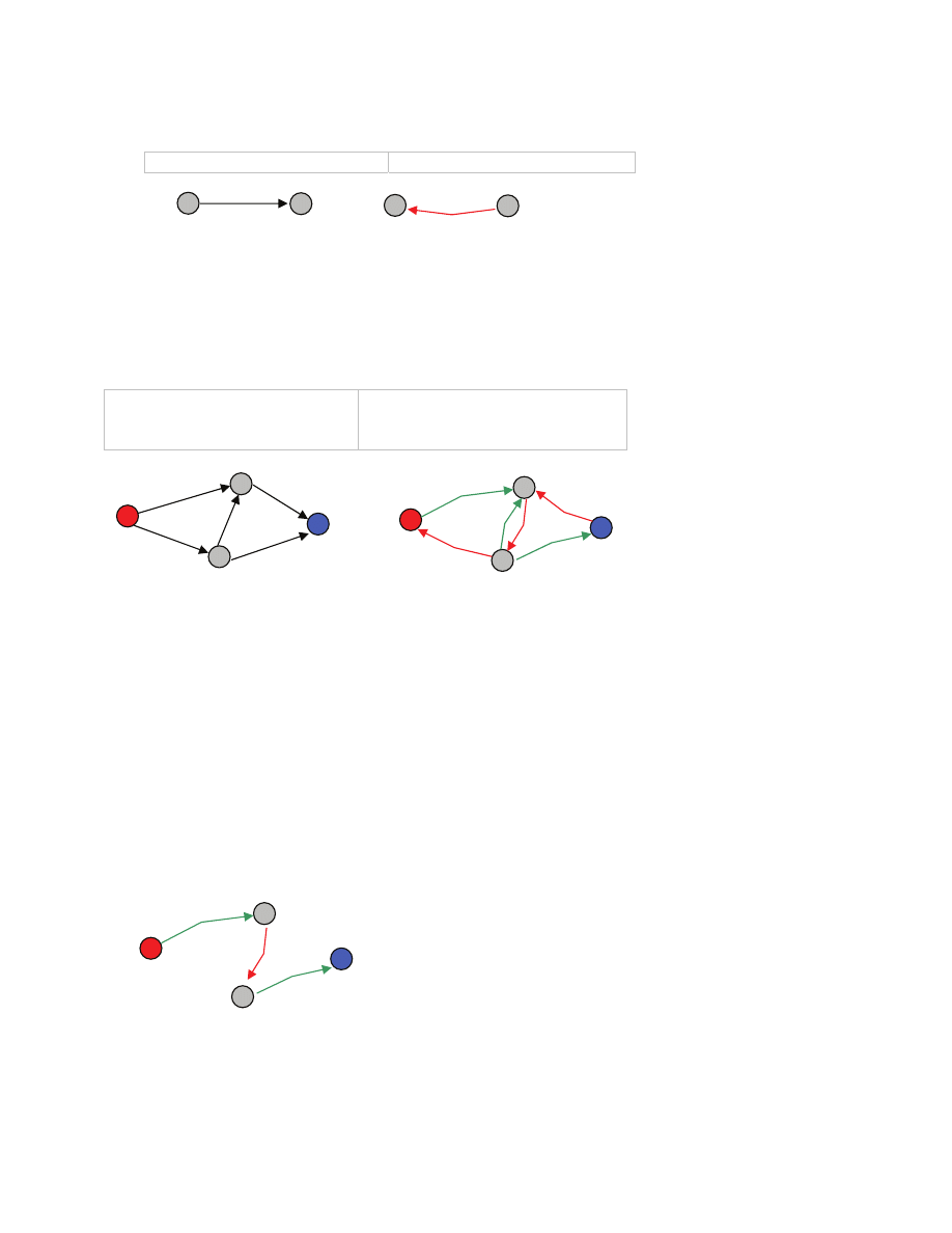
86
in G with flow f
in G
f
we call the edge added to G
f
a backward edge.
The graph G
f
is called residual graph, because it denotes, in a way, the maximum changes to the flow
that we can make along any edge in G, given the current flow f flowing through G. The residual capacity
of every edge in the residual graph is strictly greater than zero, which is an immediate consequence of
how the residual capacities were defined.
G with capacities and a flow f
residual graph G
f
with forward and backward edges
and their residual capacities
Each edge e in G
f
corresponds in a natural way to the edge in G that yielded e [[for example the two
edges (a,b) and (b,a) in G
f
correspond to the edge (b,a) in G; this notion of correspondence is useful when
G has a cycle a,b,a, because then there can be two edges from a to b in G
f
; having two edges from a to b is
formally disallowed by the definition of “directed graph” but we will allow for double edges; again
formally we would define G
f
to actually be a directed multigraph]]. Looking at the residual graph, we see
that whenever we have a forward edge [[
green
]] we have room to still push as much flow as the residual
capacity of that edge, and whenever we have a backward edge [[
red
]] we have enough flow to unpush as
much flow as the residual capacity.
[[augmentation (along an augmenting path and why this preserves flow)]]
We shall see how to modify a given flow f using the residual graph G
f
. A path v
0
,v
1
,…,v
k
in a directed
graph is called a simple path when its nodes are distinct. A simple path in G
f
from the source to the sink
is called an augmenting path.
We introduce a procedure that will modify a given flow f along a given augmenting path. Intuitively, we
will push more flow along any forward edge is P, and unpush flow along any backward edge in P. We
will make sure that we never exceed the capacity of an edge or make the flow negative. Specifically, we
u
v
2
≤
6
u
v
2
s
b
a
t
0
≤
2
6
≤
6
6
≤
8
6
≤
6
0
≤
2
s
b
a
t
2
2
6
6
2
6
s
b
a
t
2
6
2
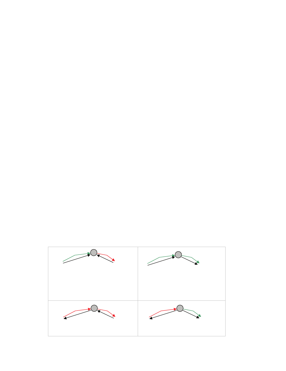
87
will pick the smallest residual capacity m along P [[number 2 in the figure]], and increase or reduce flow
by m.
Augment(f,P)
1 ► f is a flow for G and P is an augmenting path in
G
f
2 let m be the minimum residual capacity of an edge
on the path P
3 for ever edge e in P
4 let e’ be the edge in G corresponding to e
5 if e is a forward edge then
6 f(e’) ← f(e’) + m
7 if e is a backward edge then
8 f(e’) ← f(e’) - m
9 return
f
Lemma
Given a flow f for G and an augmenting path P in G
f
, the f’ returned by augment(f,P) is a flow in G.
Proof
We need to verify two requirements:
1) capacity: recall that m is the smallest residual capacity of any edge in P, we are increasing by m
the flow of forward edges and decreasing by m the flow of backward edges. But by definition of
residual capacity
a. if an edge e is a forward edge, then its residual capacity is equal to the maximum increase
of flow on the corresponding edge e’ without exceeding the capacity of e’, so increasing
the flow on e’ by m makes f(e’)
≤c
e’
.
b. if an edge e is a backward edge, then its residual capacity is equal to the current flow
value of the corresponding edge e’, so decreasing the flow on e’ by m makes f(e’)
≥0.
2) conservation: we only need to verify that the flow is conserved at any internal node of the path P.
But the path contains distinct nodes v
0
,…,v
k
and begins at the source v
0
=s and ends at the sink
v
k
=t, so any node v
1
,…,v
k-1
is internal and has a single incoming edge of the path and a single
outgoing edge of the path. We pick any such node and study four cases based on whether the
incoming and outgoing path edge is forward of backward, and depict the changes of flow on the
corresponding edges of G
a)
more flow in from the left
compensated by
less flow in from right
b)
more flow in from the left
compensated by
more flow out on the right
c)
less flow out on the left
d)
less flow out on the left
v
+m
+m
v
-m
-m
v
-m
+m
v
+m
-m
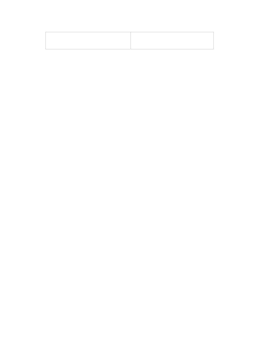
88
compensated by
less flow in from the right
compensated by
more flow out on the right
Hence the proof is completed.
█
Notice that augmentation either reduces the flow of an edge in P to 0 or saturates an edge in P [[this is the
edge in G that corresponds to the edge on the path P with minimum residual capacity]].
[[algorithm statement]]
We are now ready to present an algorithm, called Ford-Fulkerson algorithm.
Max-Flow(G)
1 for every edge e of G
2 f(e) ← 0
3 while
true
4 construct residual graph G
f
5 find a simple path P in G
f
from s to t
6 P not found?, then return f
7 f’ ← Augment(f,P)
8 f ← f’
Two main questions remain to be answered: Does the algorithm always halt? When it halts, does it
produce a flow with maximum possible value?
[[analysis of termination and running time (assuming that capacities are integers)]]
Halting and running time of the algorithm depend in a crucial way on capacities being integers. Therefore,
we assume that each edge of G has integer capacity [[so we do not allow arbitrary positive real numbers]].
We begin with an observation about values of residual capacities.
Fact
If for every edge e in G, c
e
and f(e) are integers, then every edge in G
f
has integer residual capacity at
least one.
Proof
Recall how G
f
is constructed and how the residual capacities of its edges are defined. We take an edge e
in G, and if it is not saturated, f(e)<c
e
, then we add an edge to G
f
with residual capacity c
e
-f(e), which then
must be an integer at least one. If f(e)>0, then we add to G
f
an edge with residual capacity f(e), so again
this is an integer at least one.
█
We can then show that as the algorithm iterates, the flow stays integer.

89
Lemma
Suppose that G has integer capacities, then at the beginning of every iteration of the while loop each edge
carries an integer amount of flow.
Proof
We show that the statement is a loop invariant.
At the beginning of the very first iteration, every edge carries zero amount of flow, because of the
initialization.
For the maintenance, suppose that when we are about to execute the first instruction of the body of the
while loop, every edge carries an integer amount of flow. By the Fact, then each edge of the residual
graph G
f
has integer residual capacity greater or equal to one. But then if an augmenting path is found, the
value m used by Augment(f,P) to modify the flow along edges, is an integer at least one, and so the
modified flow has integer values, too, as desired.
█
We conclude that the algorithm is making progress as it iterates.
Corollary
Suppose that G has integer capacities, then the value v(f) of flow increases by at least one after each
iteration.
Proof
Every forward edge along P increases its flow by m. We already observed that m is an integer at least one.
But P is an augmenting path, so it leaves the source and never comes back to the source. Hence P has a
forward edge e leaving the source, and any other edge along P does not enter the source. Hence after
augmentation along P, the value of the flow along e increases by m, and no other edge leaving the source
has its flow modified. So the value of the flow increases by at least one.
█
The maximum value of any flow can be bounded by the sum
∑
=
s
e
C
of
out
e
c
of capacities of edges leaving
the source.
Corollary
Suppose that G has integer capacities, then the Ford-Fulkerson algorithm performs at most C iterations.
Proof
The flow value starts at zero and gets increased by at least one in every iteration, while it cannot exceed
C.
█
Theorem
Given a flow network G=(V,E) with integer capacities, the running time of the Ford-Fulkerson algorithm
is O(|E|
⋅C).
Proof
The algorithm makes at most C iterations. Each iteration can be performed in O(|E|) time. Indeed the
graph G has |E|
≥ |V|-1 edges, because after ignoring edge orientation and possibly collapsing duplicate
edges, we get a connected undirected graph, and so that connected undirected graph must have at least as
many edges as its spanning tree i.e., at least |V|-1. Now back to the original G. The residual graph has at
most 2
⋅|E| edges, and its number of nodes is |V| which is at most |E| + 1. Hence the construction of G
f
takes O(|E|) time. Then we can find an augmenting path in G
f
in O(|V|+|E|) = O(|E|) time using BFS or
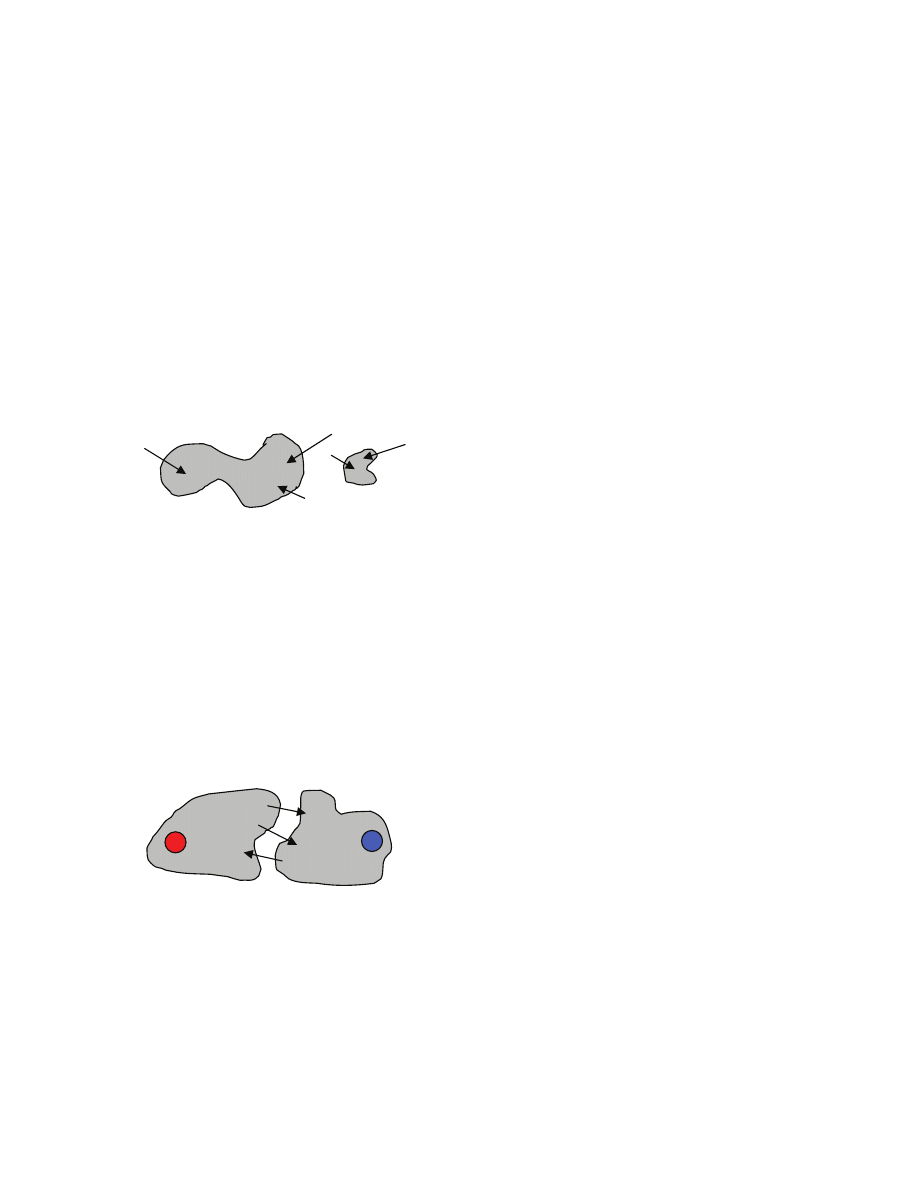
90
DFS. Augmenting along the path takes O(|V|)=O(|E|) time just by maintaining in G
f
pointers to
corresponding edges of G.
█
[[Max-Flow finds Max flow and min cut]]
We shall demonstrate now that the Ford-Fulkerson algorithm finds a maximum flow when capacities are
integers. For a moment we will relax the integrality assumption, and allow arbitrary positive real
capacities.
We being with a few definitions and properties of flows. Given a flow in G=(V,E) and a set X of nodes of
G, we define f
in
(X) as the total flow entering X, i.e., the flow on edges that begin outside of X and end in
X
( )
(
)
∑
∈
∉
∈
=
X
v
X
u
E
v
u
in
v
u
f
X
f
)
,
(
)
,
(
and f
out
(X) the total flow leaving X
( )
(
)
∑
∉
∈
∈
=
X
v
X
u
E
v
u
out
v
u
f
X
f
)
,
(
)
,
(
A cut is a partition (A,B) of nodes V such that the source belongs to A and the sink belongs to B [[similar
to the definition used for Minimum Spanning Tree]]. The capacity of a cut (A,B) is the total capacity of
edges leaving A
( )
∑
∈
∈
∈
=
B
v
A
u
E
v
u
v
u
c
B
A
c
)
,
(
)
,
(
,
Example:
cut capacity is c(A,B)=8.
Lemma 1
Given a flow f and a cut (A,B), the value of the flow v(f) is f
out
(A)-f
in
(A).
Proof
The idea is to apply the flow conservation condition inside A, and pair up certain costs, and look at edges
that do not pair up. Specifically, consider all nodes in A. Each node u other than the source satisfies the
v
u
s
t
6
2
3
A
B
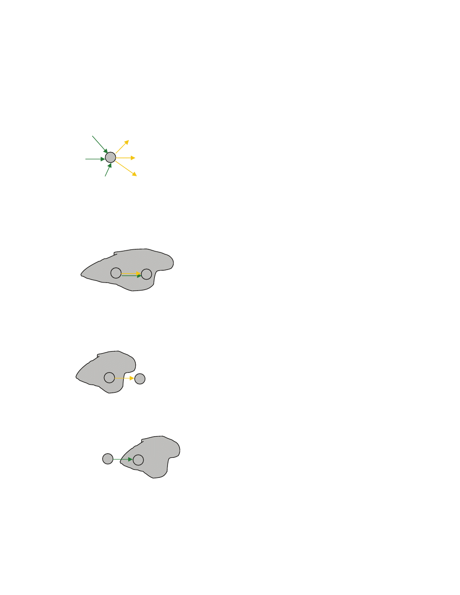
91
conservation condition f
out
(u)=f
in
(u). For the source s, we have that f
out
(s) is the value of the flow v(f) [[by
definition]], while f
in
(s)=0, since there are no edges entering s by assumption. Hence
(
)
∑
∈
−
=
A
u
in
out
u
f
u
f
f
v
)
(
)
(
)
(
Let us first look at the sum from the perspective of a node. For any u in A we add flows leaving u and
subtract flows entering u
We now look at the sum from the perspective of an edge. That is we consider every edge of E, and inspect
how much the edge contributes to the sum.
If the edge e=(u,v) has both endpoints in A, then we add f(e) when computing f
out
(u)-f
in
(u), but subtract
f(e) back when computing f
out
(v)-f
in
(v), which cancel out. So such edges contribute in total 0 to the sum.
If the edge has only u in A but not v, then we add f(e) but never subtract f(e). So such edges contribute in
total f
out
(A) to the sum.
If the edge has only v in A but not u, then we subtract f(e) but never add f(e). So such edges contribute in
total -f
in
(A) to the sum.
And finally if the edge has no endpoint in A, then we never add nor subtract f(e).
u
v
add
u
v
subtract
u
v
add
subtract
u
subtract
add

92
Hence the sum
(
)
∑
∈
−
A
u
out
in
u
f
u
f
)
(
)
(
can be represented as f
out
(A)-f
in
(A), which completes the proof.
█
Notice that every edge that crosses the cut has one endpoint in A and the other in B. So f
out
(A)=f
in
(B), and
f
in
(A)=f
out
(B). Hence v(f)=f
in
(B)-f
out
(B). In particular, if we select the cut so that B contains just the sink t,
then
Corollary
v(f) = f
in
(t)-f
out
(t).
█
But there is no edge leaving t by assumption, so f
out
(t)=0, and so
Corollary
v(f)=f
in
(t).
█
So we can compute the value of the flow just by looking at how much flow arrives at the sink [[which is
equal to how much flow departs from the source]].
Lemma
The value of any flow f is bounded by the capacity of any cut (A,B) i.e., v(f)
≤c(A,B).
Proof
Let (A,B) be any cut and f any flow. By Lemma 1,
v(f) = f
out
(A) - f
in
(A).
But f
out
(A) is at most the capacity of edges leaving A, so
v(f)
≤ c(A,B) - f
in
(A).
But f
in
(A)
≥0, so we can drop it when bounding from above, and conclude that
v(f)
≤ c(A,B)
as desired.
█
This lemma is quite significant, because if we find a flow whose value is equal to the capacity of a cut,
then the flow must have maximum value. Indeed, there cannot then be a flow with strictly larger value,
because that capacity of that cut bounds from above flow value! We now show that max flow can be
recognized by lack of any augmenting path.
Proposition
Consider a flow f. If there is no augmenting path in G
f
, then there is a cut whose capacity is equal to the
value of the flow f.
Proof
The proof approach is to find a cut whose capacity is equal to the value of the flow. Consider the set of
nodes A reachable in G
f
from the source. Let B be the set of nodes not in A. Since there is no augmenting
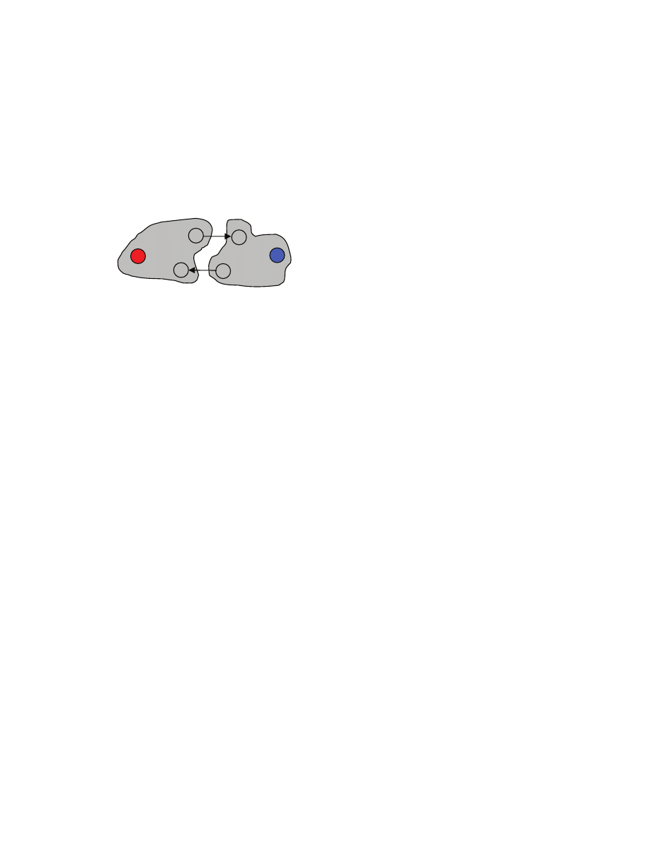
93
path in G
f
, then the sink does not belong to A. Hence (A,B) is a cut. We shall see that its capacity is equal
to the value of the flow.
What is the capacity of (A,B)? It is just the sum of the capacities of edges that leave A.
What is the value of the flow f? By Lemma, v(f) = f
out
(A)-f
in
(A).
So if we show that every edge leaving A is saturated, and every edge entering A carries zero flow, then
the proof is completed, because f
out
(A) would be the sum of capacities of edges leaving A, while f
in
(A)
would be zero.
Consider any edge (u,v) leaving A. Hence v in in B. Suppose that the edge is not saturated. So the residual
graph G
f
must contain a forward edge from u to v. But by assumption u is reachable in G
f
from the source,
and so must be v. But this contradicts the assumption that v is in B [[i.e., not reachable in G
f
from the
source]]. So indeed the edge must carry the maximum possible amount of flow in f.
Consider any edge (u’,v’) entering A. Hence v’ is in A and u’ is in B. Suppose that the edge carries a non-
zero amount of flow. But then the residual graph must contain a backward edge (v’,u’). Since v’ is in A, is
reachable in G
f
form the source, and so is then u’, contradicting the fact that u’ is in B.
█
Notice that the Ford-Fulkerson algorithm halts precisely when G
f
has no augmenting path. Hence
whenever the algorithm halts, the resulting flow f has maximum value! [[it halts with integer capacities,
but otherwise it can run arbitrarily long]]
Corollary
When it halts, the Ford-Fulkerson algorithm returns a flow of maximum value. [[it will halt when
capacities are integers, as we know]]
█
Corollary
When capacities are integers, then the Ford-Fulkerson algorithm returns a flow of maximum value in
O(C
⋅|E|) time.
█
Corollary
If every capacity is an integer, then there is a max flow that sends an integer amount of flow along each
edge [[amount can be zero]]
Proof
Because Ford-Fulkerson will halt [[by a Lemma we showed earlier]] and return an integer flow [[by a
Lemma that we showed earlier]], and that flow is maximal [[by a Corollary]].
█
s
t
A
B
u’
v’
u
v
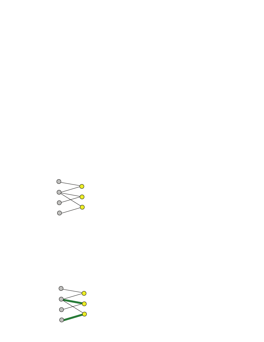
94
Theorem (Max-Flow Min-Cut Theorem)
The value of a maximum flow is equal to the minimum capacity of any cut.
Proof
There exists a flow f with maximum value v(f) [[simply because value is a continuous function defined
over a closed domain]]. Then G
f
cannot have any augmenting path [[otherwise flow value could be strictly
increased]]. But then by the Lemma there is a cut (A,B) with capacity v(f). No cut (A’,B’) can have
strictly smaller capacity, because, by a Lemma, any flow value [[in particular v(f)]] bounds from below
any cut capacity [[in particular c(A’,B’)]].
█
When capacities are real numbers, we cannot guarantee that the Ford-Fulkerson algorithm will halt. In
fact one can select capacities and steer the selection of augmenting paths while the algorithm is running,
so that the algorithm will run arbitrarily long. Note that when capacities are rational numbers [[fractions]]
then Ford-Fulkerson can still be applied just be multiplying out by Least Common Multiplier of the
denominators.
4.6 Maximum matchings in bipartite graphs
Let us revisit the problem of matching people up. Suppose that we have a set X of males and a set Y of
females. For every male x and female y, we can determine if they like each other or not (because the
female does not like the male, or the male does not like the female, or they both do not like each other)
[[for simplicity of presentation, we only consider matching males with females]]. We can represent the
situation as an undirected graph
where set there is an edge between x
∈X and y∈Y exactly when x and y like each other. Notice that there
are no edges between nodes on X, nor are there edges between nodes of Y [[again, the heterosexual
scenario]]. An undirected graph G=(V,E) whose nodes can be partitioned into X and Y, so that any edge
has one endpoint in X and the other in Y is called bipartite.
We would like to find out whom to match up with whom, so as to maximize the number of pairs. Of
course, any male can be matched up to at most one female, and any female can be matched up to at most
one male [[recall the definition of a matching presented earlier in the course]]. Here is an example of a
matching (
green
)
Y
X
Y
X
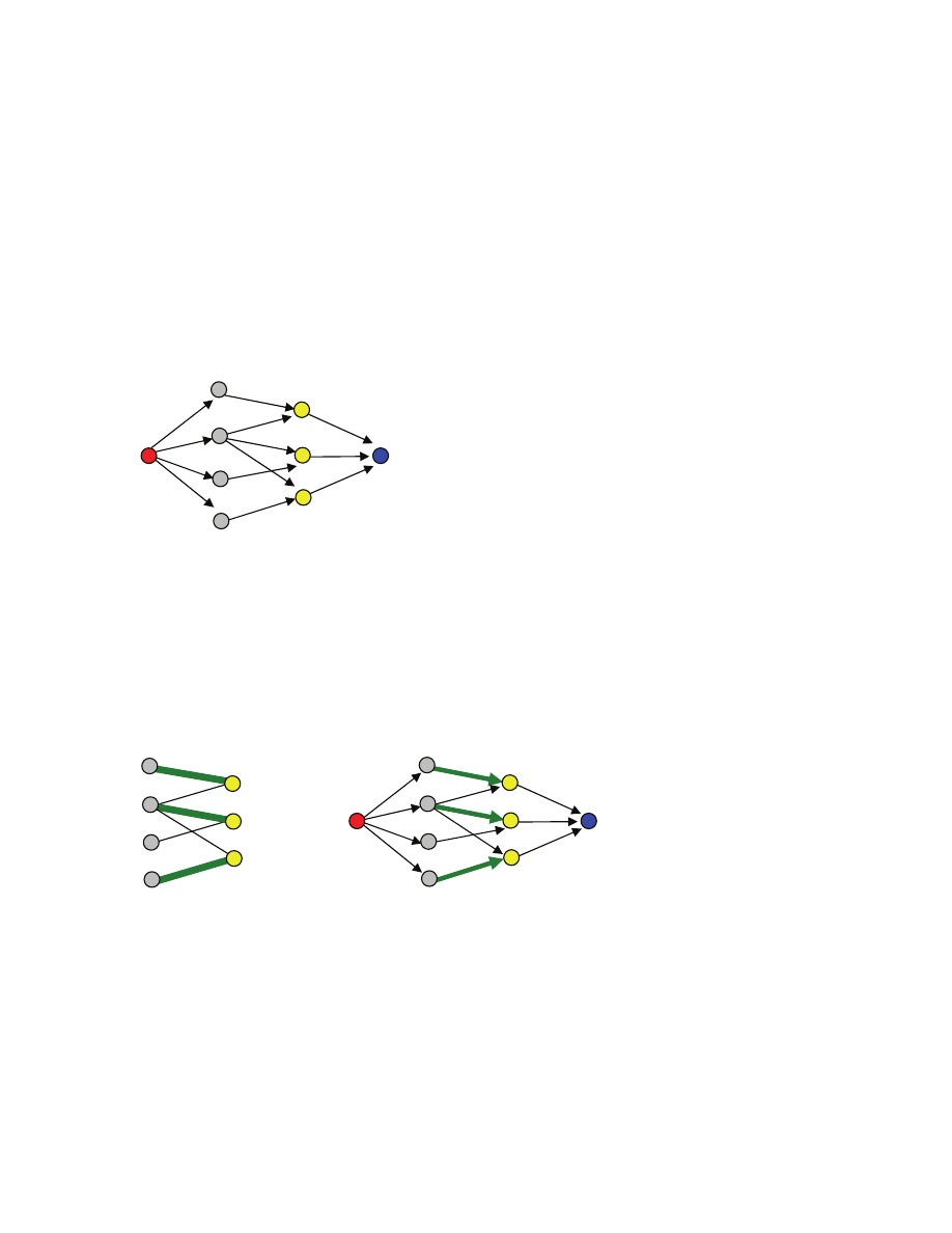
95
That matching is not maximum size, because it is possible to match up three pairs.
[[Algorithm]]
Our algorithm for producing a maximum matching in a bipartite graph will use a maximum flow
algorithm. We take the bipartite graph G, and construct a flow network G’. Specifically we transform G
into a directed graph by orienting its edges toward right, and adding a
source
s on the left and a
sink
t on
the right. The source has an edge to each node from X, and each node from Y has an edge to the sink. We
set the capacity of every edge to
1 [[green]]
.
We shall see that any matching of size k yields a flow of value k, and any flow of value k yields a
matching of size k. Hence maximum flow value is equal to the maximum size of a matching. Moreover,
our proof will let us construct a maximum matching from a maximum flow.
Lemma
If M is a matching of maximum size k in G, then there is a flow of value k in G’.
Proof
Consider the edges in G’ corresponding to the edges in the matching M.
Set the flow value on each such edge of G’ to 1. Since every x
∈X can be matched with at most one
element of Y, the flow leaving x is at most one. Since every y
∈Y can be matched with at most one
element of X, the flow entering y is at most 1. Hence we can push one unit of flow from s to every
matched element of X, and push toward t one unit of flow from every matched element of Y, thus
ensuring the flow conservation and capacity conditions.
Y
X
s
t
≤1
≤1
≤1
≤1
≤1
≤1
≤1
≤1
≤1
≤1
≤1
≤1
≤1
Y
X
Y
X
s
t
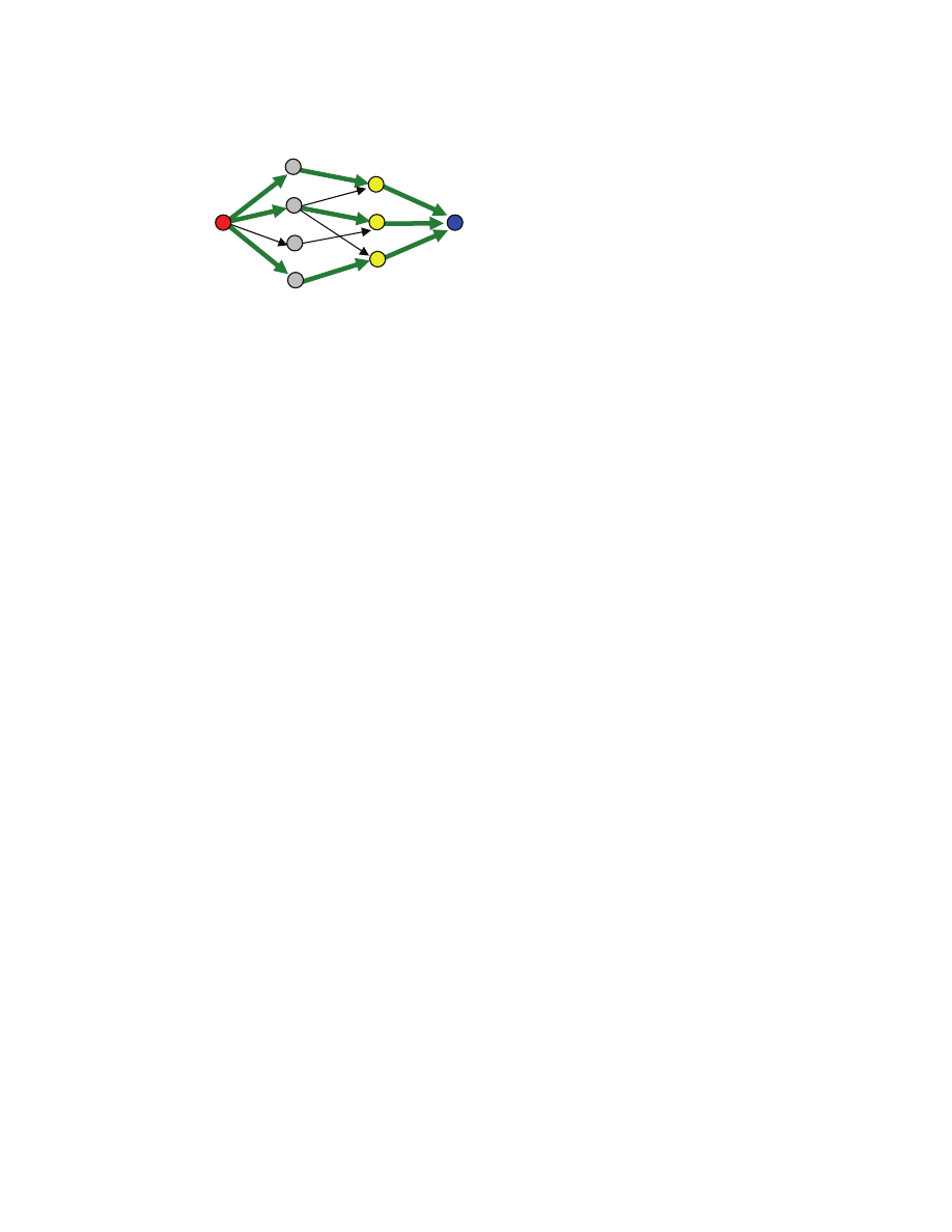
96
Thus there is a flow in G’ with value k.
█
Lemma
If maximum flow in G’ has value k, then there is a matching of size k.
Proof
Let k me the maximum flow value in G’. Since G’ has integer capacities, we know that there is a flow f
that sends an integer flow amount along every edge [[we proved this when analyzing Ford-Fulkerson
algorithm]]. But capacities are 1, so the flow f sends, along every edge, either 0 or 1 units of flow. Let M
be the set of edges from X to Y each carrying one unit of flow. We verify that the edges form a desired
matching:
1) there must be exactly k such edges. Indeed let A={s}
∪X. Now the value k of the flow f is equal
to f
out
(A)-f
in
(A), but there are no edges entering A, and so f
out
(A)=k. But each edge leaving A
carries either zero or one unit of flow, so indeed there are k edges in M.
2) there is at most one edge of M leaving any given element of X. We cannot have 2, because this
would mean that at least two units of flow leave a node of X, while that node can receive at most
one unit of flow because it has only one incoming edge and the capacity of that edge is 1.
3) there is at most one edge of M entering any given element of Y. Similar argument, but now it
would mean that two units of flow are entering a node of Y, while only one unit can leave,
because there is just one leaving edge, and it has capacity 1.
█
Corollary
A maximum matching in G can be constructed by running Ford-Fulkerson algorithm on the graph G’, and
selecting the edges between X and Y carrying one unit of flow.
█
Recall that given a flow network G=(V,E) with integer capacities, the Ford-Fulkerson algorithm returns a
maximum flow in O(C
⋅|E|) time, where C is the maximum value of any flow. In our case C is bounded by
the minimum of |X| and |Y|.
Theorem
A maximum matching in a bipartite graph G=(X
∪Y,E) can be found in time O(min{|X|,|Y|}⋅|E|).
█
Y
X
s
t
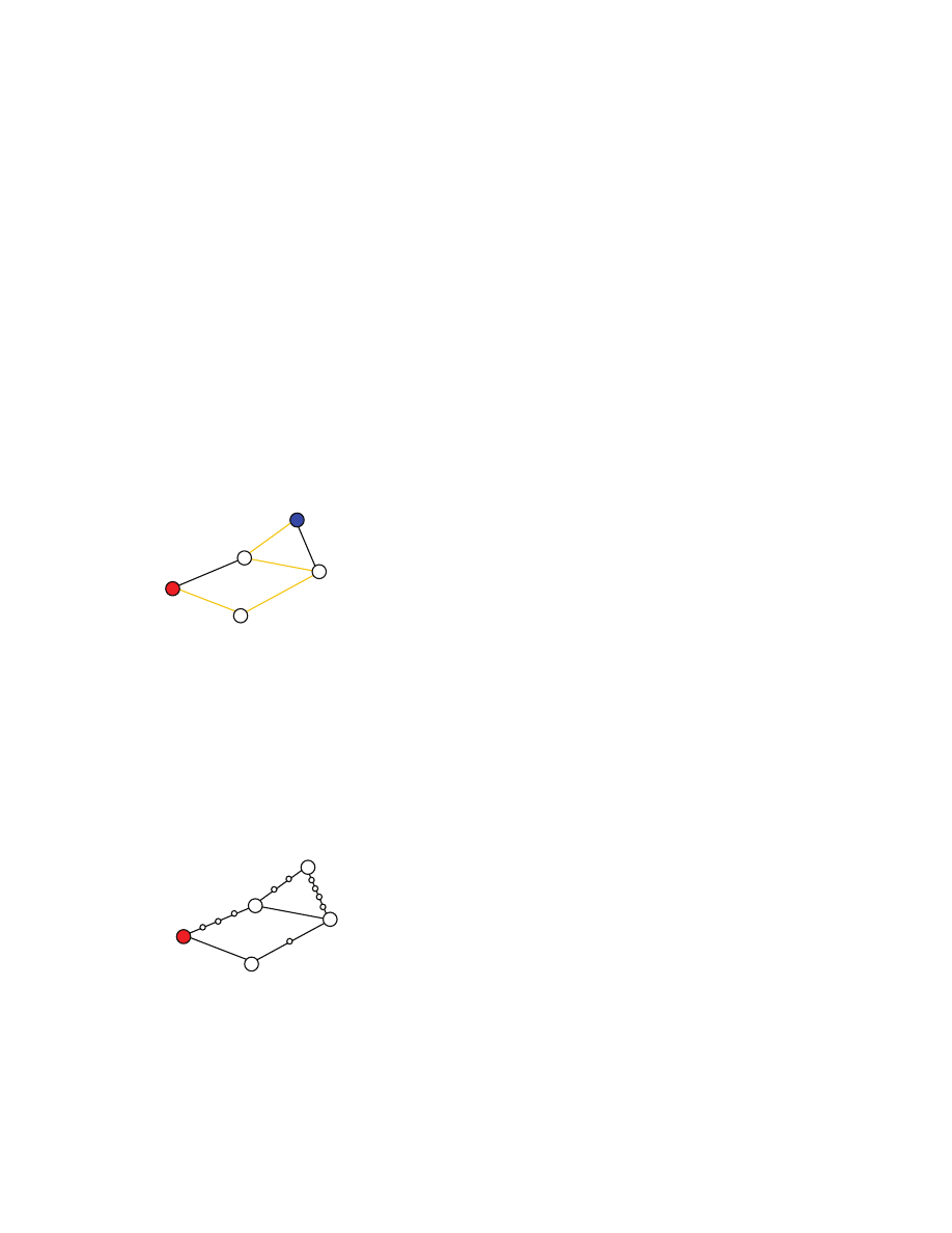
97
4.7 Shortest Paths
4.7.1 Dijkstra’s algorithm
Imagine that we have a collection of cities and some pairs are connected by a direct road. For each road
connecting two cities, say u and v, we have the time of traveling from u to v, equal to the time of traveling
in the reverse direction from v to u. We are given a starting city s and a destination city t, and want to
compute a shortest path from s to t i.e., a path that would take us the least time to travel from s to t.
We can model the problem as an undirected graph G=(V,E), where each edge e
∈E has length c
e
that is at
least zero [[i.e., non-negative]]. We are given node s and t from V, and want to find a shortest path from s
to t. [[Recall that a path is a sequence of nodes connected by edges, in the example below s,a,c,b,t is a
path; the length of a path is the sum of the lengths of the edges along the path; distance from u to v is the
lengths of a shortest path from u to v]]. For example a shortest path from s to t in the following graph is
the
yellow
one, and it has length 7 [[there is another path of the same length from s to t]].
We shall see that there is a very simple greedy algorithm that solves the shortest path problem. As a
matter of fact the algorithm will solve a more general problem: given s, find a shortest path from s to any
node in V [[in particular to t, too]].
First approach: reduction to BFS
The shortest paths problem can be easily solved using tools that we have already developed. Recall that
BFS finds shortest paths in a graph whose each edge has length one. Hence we can replace each edge e
with length c
e
≥1 with c
e
edges; if two nodes are linked by a zero length edge, then we “merge” the nodes
into a single node; we then run BFS on the resulting graph.
Unfortunately, this approach has disadvantages: (1) the edge lengths must be integers, (2) the resulting
number of edges may be large---it is as large as the sum of the lengths of the edges in E. Suppose that an
edge has length 2
60
, then BFS may run for a very long time! However, there is an algorithm that
generalizes BFS such that the running time does not depend on the sum of edge lengths.
s
4
2
1
1
5
3
t
s
a
b
c

98
Second approach: generalization of BFS
We will maintain a set S of nodes for which we have already computed distance from s and a shortest
path. We will store distances from s in a table d[] and shortest paths from s in a table P[]. Initially S={s},
d[s]=0, and P[s]=s. The algorithm will be iteratively adding nodes to S and updating tables d[] and p[], as
long as the cardinality of S is smaller than the cardinality of V.
In each iteration we assume that we have computed the distance d[u] from s to u, for every node u in S,
and a shortest path, P[u], from s to u. Within an iteration, we consider the set of nodes
W
that are not in S,
but have an edge leading from a node in S
Let
U(w)
be the set of nodes from S that have an edge leading to w. One way to get from s to w is to
follow the path
P[u]
from s to
u
∈U(w) and then continue along the edge u-w. Let us call the resulting
path Q
u,w
; its length is d[u]+c
u-w
. We select w’ and u’ to minimize the length of the path Q
u’,w’
i.e., select
u’ and w’ so that
{
}
w
u
w
Q
u
W
w
w
u
c
u
d
c
u
d
−
∈
∈
−
+
=
+
]
[
min
]
'
[
)
(
,
'
'
We then add w’ to S, set d[w’] to d[u’]+c
u’-w’
, and define the path P[w’] to be P[u’] followed by the node
w’.
Dijkstra’s Algorithm(G,s)
1 S
← {s}
2 d[s]
← 0
3 P[s]
← s
4 while |S| < |V|
5 let W = {w: w∉S and there is an edge u-w with u∈S}
6 let U(w) = {u: u∈S and there is an edge u-w}
7 find w’∈W and u’∈U(w’) so that
{
}
w
u
w
Q
u
W
w
w
u
c
u
d
c
u
d
−
∈
∈
−
+
=
+
]
[
min
]
'
[
)
(
,
'
'
8 S ← S∪{w’}
9 d[w’] ← d[u’]+c
u’-w’
10 P[w’] ← P[u’],w’
We shall now show that the algorithm is correct. That is that it computes a shortest path from s to any
node of G.
S
w
s
U(w)
P[u]
u
W
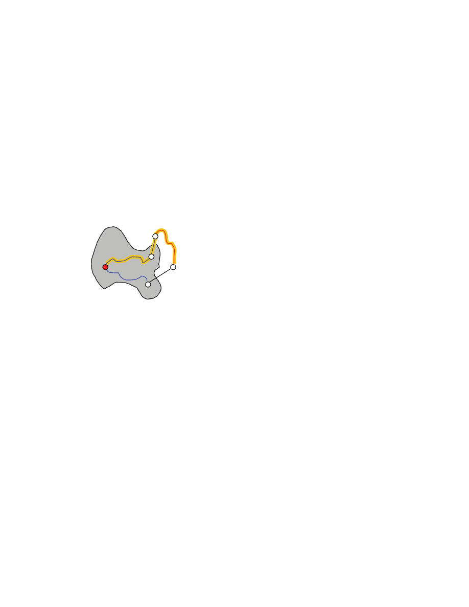
99
Lemma
Let G be a connected graph and every its edge has length at least zero. At the end of every iteration of the
while loop, the set S has the property that
• S is not empty
• for any u∈S, d[u] is the distance from s to u and P[u] is a shortest path from s to u.
Proof
The proof is by induction. The claim is clearly true at the end of iteration number zero [[i.e., at the
beginning of the first iteration]], by the way S, d[s] and P[s] were initialized.
For the inductive step, assume that at the beginning of an iteration, the set S has the property that for any
u
∈S, d[u] is the distance from s to u and P[u] is a shortest path from s to u. We shall see that at the end of
the iteration the set S has that property, too [[we are adding w’ to S in that iteration]].
Since |S|<|V|, there is at least one node outside of S. But G is connected, so the set W has at least one
node. But S is not empty, so for any w
∈W, the set U(w) is not empty, either. Let u’ and w’ be the nodes
as defined in the algorithm. We will argue that any path from s to w’ has length at least d[u’]+c
u’-w’
, which
will complete the inductive step.
Consider any path
P
from s to w’. That path must at some point leave S, because s is in S, but w’ is not in
S. Let y be the first node outside of S along the path, and x the preceding node. We can then split the path
into the part L from s to y, and the remaining part R from y to w’. We shall see that the length of P is at
least the length of the path P[u’],w’. First note that
length of L
≥ d[x]+c
x-y
simply because d[x] is by inductive assumption the distance from s to x [[the length of a shortest path
from s to x]] while the prefix of P from s to x is just one path from s to x. But y is in W and x is in U(y) so
d[x] + c
x,y
≥ d[u’] + c
u’,w’
by the way we selected u’ and w’. Hence we conclude that the prefix of P from s to y has length at least
the length of the path P[u’],w’. But the length of R has to be at least zero, because each edge has non-
negative length. Therefore
length of P
≥ length of P[u’],w’.
Since P was an arbitrary path from s to w’, we conclude that P[u’],w’ has the shortest length, and so d[w’]
and P[w’] are appropriately set to the distance from s to w’ and a shortest path from s to w’ respectively.
█
S
w’
u’
s
L
P
u’
x
y
R
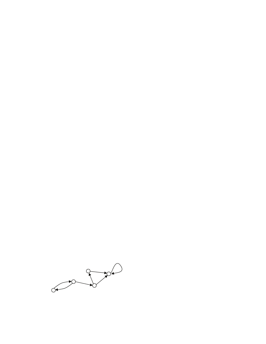
100
Implementation details
We need to maintain the set of nodes W so that we can quickly select w’. We use the min-heap data
structure for this purpose. Each heap element will be a triple (key,node,edge). We begin by inserting into
the heap all nodes v that neighbor node s i.e., we insert triples (c
s-v
, v, s-v) for every node v such that
there is an edge s-v. We color every node white, except for s that is black. In each iteration we keep on
removing a triple with minimum key, say this triple is (c
u’,w’
, w’, u’-w’), until w’ is white. We then set the
color of w’ to black, d[w’] to d[u’]+c
u’-w’
and define the path P[w’] to be P[u’],w’. We then consider every
edge w’-y out of w’ leading to a white node y. If the (white) node y is in the heap [[for every graph node,
we keep a pointer to the triple in the heap containing the node]], we check if the key of the triple
containing y is strictly greater than d[w’]+c
w’-y
, and if so, we remove the triple and add the triple
(d[w’]+c
w’-y
, y, w’-y) instead [[updating the pointers]]. If, however, the (white) node y is not in the heap,
we simply insert the triple (d[w’]+c
w’-y
, y, w’-y) into the heap.
Theorem
The Dijkstra’s algorithm can be implemented to run in O(|E|
⋅log|E|) time.
Proof
We use aggregate counting. As we iterate, for any node, we consider at most every edge leading out of the
node, and then perform at most one heap removal and insertion for that edge.
█
4.7.2 Directed acyclic graphs with possibly negative edge lengths
Let us revisit our initial motivation for computing shortest paths. We then considered a collection of cities,
some pairs of cities were connected by a direct road, and for each road connecting cities, say u and v, we
had a time of traveling from u to v, same as the time of traveling in the opposite direction. We modeled
this scenario as an undirected graph where every edge had an associated number called length. Unlike in
that scenario, suppose now that traveling along a road comes at a cost (say the gas consumed by the car),
but may yield some benefit (the beautiful places you see on the way), and so we have a net loss associated
with each road equal to the cost minus the benefit, that may be positive, negative or zero. Moreover, it
could happen that the net loss of traveling from u to v is different from the net loss of traveling in the
reverse direction (say we go uphill from u to v, but downhill from v to u). In this new setting, as before,
we are interested in computing a “shortest” path from a given city to a given city.
We model the new problem as a directed graph G=(V,E), such that each edge uÆv has a length c
u
Æ
v
that
is an arbitrary real number (positive, negative, or zero). As before, the length of a path is the sum of
lengths of the edges along the path, and the distance from u to v is the length of a shortest path from u to v
[[can be plus or minus infinite, see explanations next]]. Let us consider an example problem instance and
see what a shortest path could be.
Let us consider an example graph G with edge lengths as follows
We want to compute a shortest path from a node to a node. What difficulties could we encounter?
2
4
a
d
b
c
-3
-5
2
e
0
1
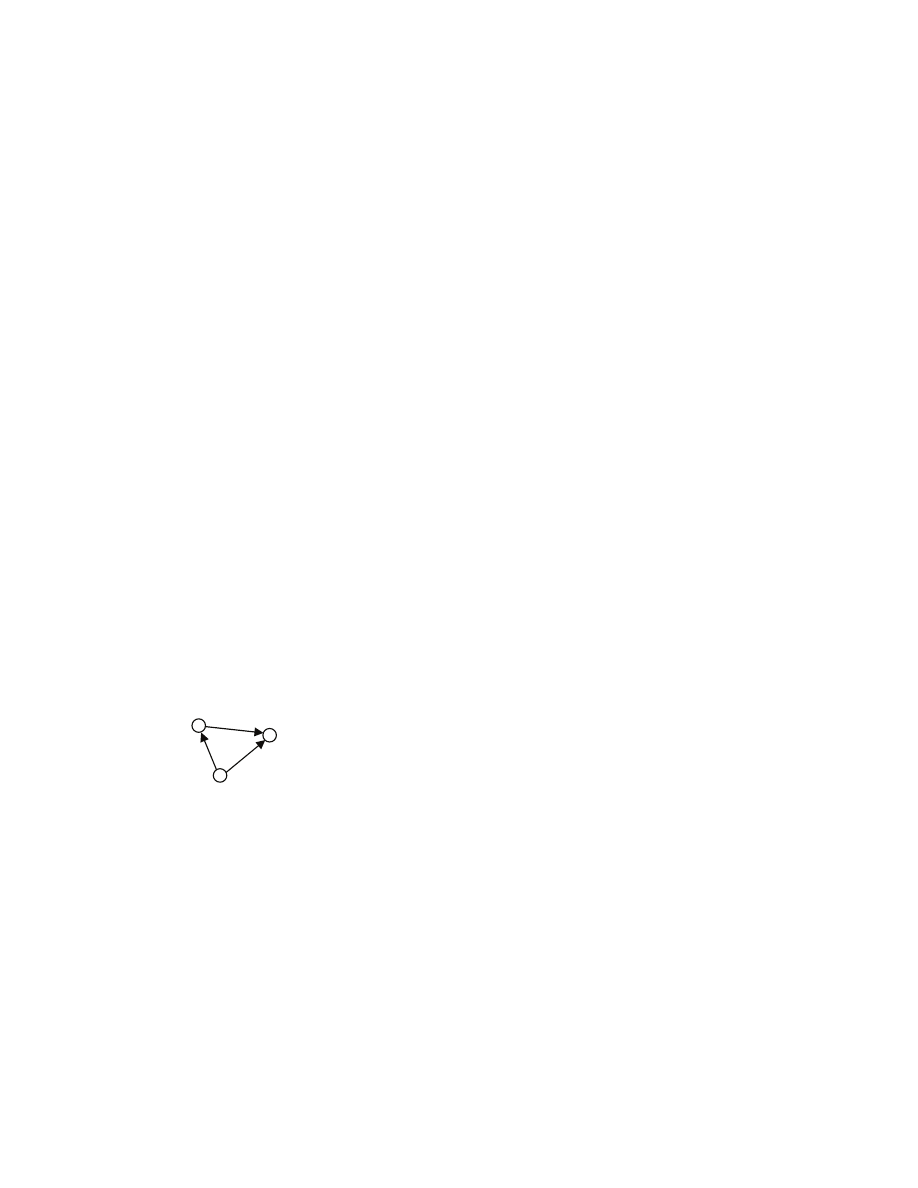
101
• First difficulty: it could be that there is no path. For example there is no path from c to b. When
there is no path from node u to node v, then we define the distance from u to v as plus infinity.
• Second difficulty: it could be that there is a path of arbitrary low length. For example, we can get
from a to b along a path a,b of length 2, but also along a path a,b,a,b, of length 1, but also along
the path a,b,a,b,a,b of length 0, but also a,b,a,b,a,b,a,b of length -1, and so on, thus by looping
between a and b arbitrary many times we can produce a path from a to b of arbitrary low length!
When there is a path from node u to node v of arbitrary small length [[i.e., for any number, there
is a path of length at most that number]], then we define the distance from u to v as minus
infinity.
The lesson from this example is that finding shortest paths in graphs with possibly negative edge lengths
seems more difficult than searching for such paths when edge lengths are non-negative. Let us try to
design an algorithm.
First approach: generalization of Dijkstra’s algorithm
Let us try to use the greedy approach of the Dijkstra’s algorithm, and see why it does not work. Focus on
the node c, and let us try to compute a shortest path to node d. Like in Dijkstra’s algorithm, we begin with
S={c}, and look for a closest node outside of S. Such node is d, whose believed distance from c is 2, and
so we add d to S. Now S={c,d}. Note that we would not add e to S instead, because e was strictly further
from S than d was. Observe, however, that it is shorter to go from c to d through e, because although we
are initially traveling along an edge of length 4, which is longer than 2, but then we follow an edge of
length -5, for the total of -1. So another lesson from this example is that we must be more careful than in
Dijkstra’s algorithm, because a choice of a path that initially seems bad, may turn out to be very good
when further down the path we encounter edges of low length, while a path that initially looks good may
turn out to be bad after all.
Second approach: increase lengths to get rid of negative ones
A natural way to deal with negative edge lengths is to increase the length of every edge by sufficiently
large number. This, however, would not work because paths may have different number of edges. Say
here, the shortest path from c to d is through e, but after we increase lengths by 3, that path has length 2,
while the direct edge from c to d has length just 0.
We thus need a different approach. Before we start designing an algorithm, let’s record a useful property
of any shortest path.
Lemma (Subpath lemma)
Suppose that there exists a shortest path P from node u to node v [[could be that u=v]], P=u
0
,u
1
,…,u
k
,
u
0
=u and u
k
=v, k
≥0, in a directed graph G=(V,E) where each edge e has length c
e
that is a real number
(possibly negative). Then any subpath of P is a shortest path i.e., for any 0
≤i<j≤k, the path P
i,j
=u
i
,…,u
j
is a
shortest path from node u
i
to node u
j
.
Proof
Since P is a shortest path from u to v, no path can be shorter. Suppose, by way of contradiction, that P
i,j
is
not a shortest path from u
i
to u
j
. So there is a path P’ from u
i
to u
j
that is strictly shorter than P
i,j
. But then
the path u
0
,…,u
i-1
,P’,u
j+1
,…,u
k
leads from u to v, and is strictly shorter than the path P. This contradicts
the fact that P is a shortest path from u to v. █
-2
d
c
-2
-3
e

102
Our eventual goal is to design a shortest path algorithm for an arbitrary directed graph. However, we will
first focus on simpler graphs: directed acyclic graphs (dags).
Shortest paths in dags
A dag simplifies the problem of finding shortest paths because of lack of cycles. In the problem for
general directed graphs we could have two nodes u and v such that there is a path from u to v with
arbitrary low length [[minus infinite distance]]. However, in a dag this is not possible. Indeed any path
u
0
,…,u
k
can have at most |V| nodes, just because dag has no cycles [[if a path was to more than |V| nodes,
then two would be the same and so we would have a cycle]].
Corollary
If G=(V,E) is a dag with edges having lengths that are arbitrary real numbers, then for any nodes u,v
∈V,
either
• there is no path from u to v in G, in which case the distance from u to v is infinite, or
• there is a shortest path from u to v in G [[in which case the distance is a real number]],
• but there cannot be an arbitrary short path [[the distance cannot be minus infinity]].
█
Let us outline how the algorithm works. We start with a directed acyclic graph G=(V,E). The algorithm
maintains two tables d[] and P[]. The entry d[u] will become the distance from a given node s to u, and
when d[u]<
∞ then P[u] will be a shortest path from s to u. The algorithm uses a greedy approach. Let
u
1
,…,u
|V|
be a topological sort of G. The algorithm scans the topological sort from left to right, and when
visiting node u
j
, the algorithm sets d[u
j
] and possibly P[u
j
]. For any node u
∈V, let B(u) be the set of nodes
that have an edge leading to u, that is B(u) = {v
∈V : vÆu is an edge in E} [[the set of “parent” nodes, or
“backnodes”]]. Then the algorithm finds a shortest path to u
j
, leading through a node in B(u
j
), and updates
d[u
j
] and P[u
j
] when such path exists [[very much like Dijkstra’s algorithm, only that there are fewer
choices, as we consider just one node, u
j
, at a time, while Dijkstra’s algorithm may consider more, when
more are outside of S]].
Dag-Shortest-Paths(G,s)
1 let
u
1
,…,u
|V|
be a topological sort of G
2 find m such that u
m
=s
3 set d[u
1
]=…=d[u
m-1
] ← ∞ , and d[u
m
] ← 0
4 for j=m+1 to |V|
5 let B(u
j
) = {v: there is an edge vÆu
j
}
6 if d[v]=∞ for all v∈B(u
j
) then
7 d[u
j
] ← ∞
8 else
9 find v’∈B(u
j
) such that
{
}
u
v
u
B
v
u
v
c
v
d
c
v
d
j
j
→
∈
→
+
=
+
]
[
min
]
'
[
)
(
'
10 d[u
j
] ←
j
u
v
c
v
d
→
+
'
]
'
[
11 P[u
j
] ← P[v’],u
j
The following lemma settles correctness of the algorithm.
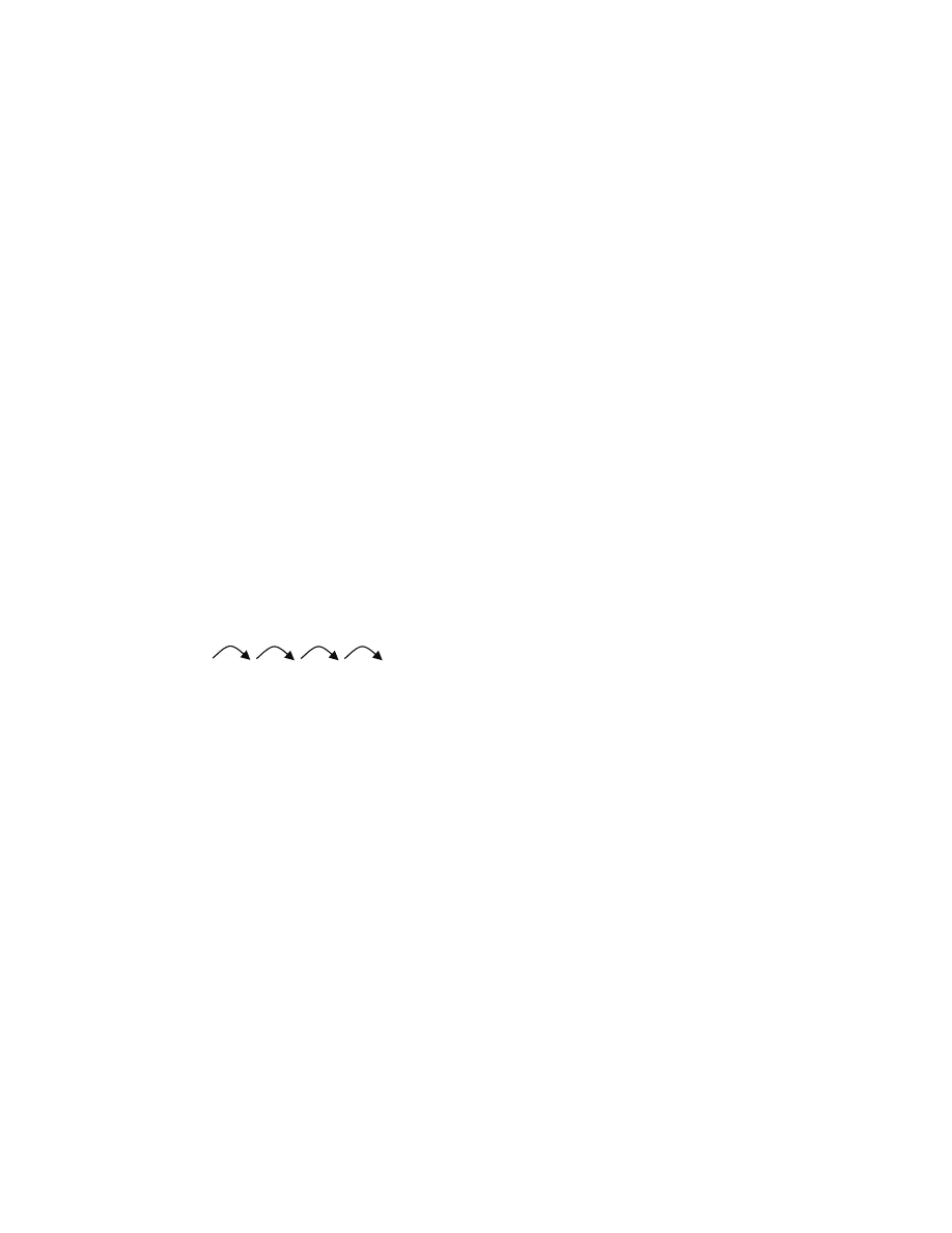
103
Lemma
When the algorithm halts, for any u
i
, 1
≤i≤|V|, d[u
i
] is equal to the distance from s to u
i
, and when the
distance <
∞, then P[u
i
] is a shortest path from s to u
i
.
Proof
The algorithm keeps on increasing j in every iteration. We shall show that at the end of each iteration, for
all 1
≤i≤j, d[u
i
] is the distance from s to u
i
.
For the base case, suppose that no iteration has yet been performed and we are entering the loop. We want
to show that for all 1
≤i≤m, d[u
i
] is the distance from s to u
i
, But there is no path from s to any node to the
left of s in the topological sort. So the distance from s to any such node is infinite. How about the node s
itself? There is just one path from s to s, namely the path s [[again because G is a dag]], and the length of
that path is zero. Hence the content of d[] and P[] is correct.
For the inductive step, consider any j>m and the iteration when node u
j
is being considered. By the
inductive assumption, d[u
i
] is the distance from s to u
i
, for all 1
≤i<j, and when d[u
i
]<
∞, then P[u
i
] is a
shortest path from s to u
i
. In that iteration we set the value of d[u
j
] and possibly of P[u
j
]. We want to show
that the resulting value of d[u
j
] is exactly the distance from s to u
j
, and when d[u
j
]<
∞ then P[u
j
] is a
shortest path from s to u
j
. The Corollary ensures that there are two cases to consider.
Case 1: Suppose first that there is no path from s to u
j
. But then there is no path from s to any node in
B(u
j
). So at the time of the iteration, by the inductive assumption, d[v]=
∞ for any node v∈B(u
j
). Hence in
the iteration d[u
j
] gets set to plus infinity, as desired.
Case 2: Suppose, on the other hand, that there is a shortest path from s to u
j
. Since s in not u
j
, the path has
at least two nodes. Denote the path by v
0
,v
1
,…,v
k
,u
j
with k
≥0 and v
0
=s, and let L be the length of the path.
We first show that the algorithm can make a good choice. There is an edge v
k
Æu
j
, and so v
k
is to the left
of u
j
in the topological sort. But by the subpath lemma, the path v
0
,..,v
k
is a shortest path from v
0
to v
k
, and
so by the inductive assumption d[v
k
] is the length of the path. So
j
k
u
v
k
c
v
d
→
+
]
[
is equal to the length L of
a shortest path from s to u
j
. Now v
k
∈B(u
j
), so the algorithm considers v
k
as a candidate for v’ in the
iteration.
The algorithm picks a node v’ from B(u
j
) that minimizes
j
u
v
c
v
d
→
+
'
]
'
[
. It must therefore pick a node v’
such that
j
u
v
c
v
d
→
+
'
]
'
[
≤ L. In particular d[v’]<∞, and so by the inductive assumption there is a shortest
path from s to v’. Hence the path along with the node u
j
, form a path from s to u
j
of length at most L, thus
the shortest. Hence d[u
j
] is set to L<
∞ and P[u
j
] is set to P[v’],u
j
which is a shortest path from s to u
j
.
█
Implementation details
A topological sort can be constructed in time O(|V|+|E|) using a modified DFS, as we have seen earlier in
the course. We can compute backlinks pointing to any node just by scanning all edges of G, and for any
… v
0
… v
1
… v
2
… v
k
… u
j
…
||
s
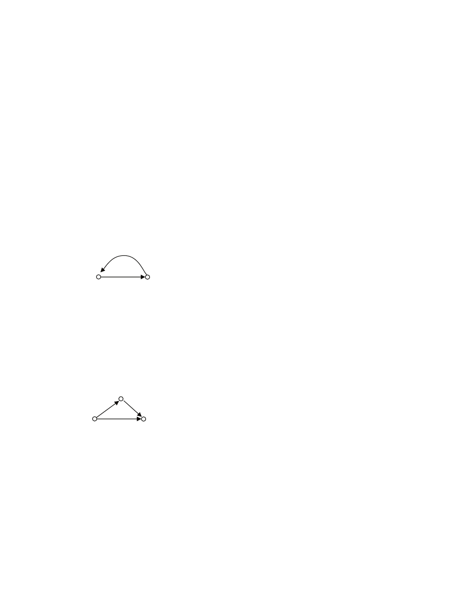
104
edge uÆv adding u to the adjacency list of backlinks to v. Backlinks are useful because we can then
quickly obtain the sets B(u
j
). It is clear that in the for loop we inspect each backlink at most once. We can
represent the table P[] in O(|V|), just be storing, for each node, a pointer to the previous node on the path,
and then when we need to construct a path from s to u, we start at u and follow the pointers.
Theorem
Given any dag G=(V,E) where each edge has length that is an arbitrary real number, and a node s of G,
we can compute in O(|V|+|E|) time the distance from s to any node of G and a shortest path to that node if
such path exists.
█
4.7.3 Bellman-Ford
We have seen that when a directed graph has no cycles (is a dag) then we can compute shortest paths even
if edges have negative lengths. We were able to perform the computation using a greedy algorithm that
sweeps through a topological sort of the graph, in a fashion somewhat resembling the Dijkstra’s algorithm.
However, our algorithm was somewhat restricted because the graph could not have any cycles. What can
we do if a graph contains a cycle?
Can we compute the distance from s to every other node? We shall see that we can indeed compute
distance even when the graph has cycles. The algorithm will use a very powerful technique called
dynamic programming. In essence, the algorithm will compute distance from s to a node u recursively.
We will be able to evaluate the recurrence efficiently by storing previous evaluations in memory, and
using them whenever we need to evaluate the recurrence again.
Consider a directed graph G=(V,E) [[may have cycles]] where each edge has length [[possibly negative]].
Let Q(s,u,i) be the set of all paths from s to u that have at most i edges, for any node s and u and i
≥0
[[possibly u=v]]. Example
Then
Q(s,u,0) = {}
Q(s,u,1) = { s,u }
Q(s,u,2) = { s,u ; s,w,u }
Q(s,u,3) = { s,u ; s,w,u }
Let OPT(s,u,i) be the minimum length of a path in the set Q(s,u,i)
)
(
min
)
,
,
(
)
,
,
(
P
lenght
i
u
s
OPT
i
u
s
Q
P
∈
=
2
-2
1
w
u
s
-1
u
s
3
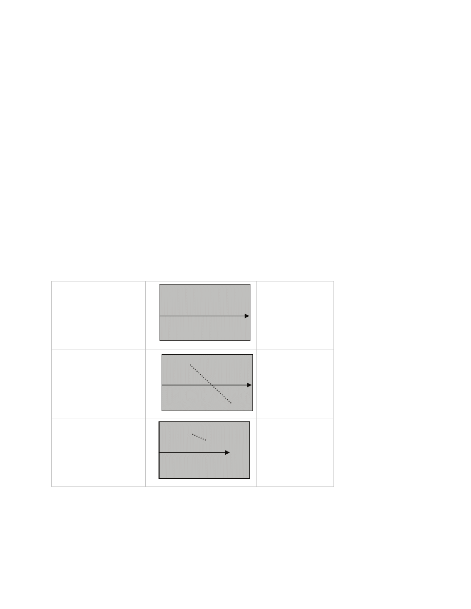
105
By convention, min of an empty set is defined to be plus infinity. In particular OPT(s,s,0)=0, but when
s
≠u, then OPT(s,u,0)=∞ [[in order for a path with at most zero edges to even exist from s to u, it must be
that s=u]].
Then
OPT(s,u,0) =
∞
OPT(s,u,1) = 1
OPT(s,u,2) = 0
OPT(s,u,3) = 0
Fact
For any s and u, OPT(s,u,0)
≥ OPT(s,u,1) ≥ OPT(s,u,2) ≥ OPT(s,u,3) ≥ … [[just because any path of
length at most i is a path of length at most i+1, and we are minimizing]]
█
Why is the concept of OPT(s,u,i) useful? Suppose for a moment that we just want to find the length of a
shortest path from s to u, not a shortest path itself. It turns out that by inspecting OPT(s,u,i) for different i,
we can determine the length of a shortest path from s to u [[with a bit more work we will be able to
determine a shortest path itself]]. The sequence OPT(s,u,0), OPT(s,u,1), OPT(s,u,2), OPT(s,u,3), … can
evolve in three qualitatively different ways:
no path exists
from s to u
always plus infinity
arbitrarily short path
from s to u exists
tending to minus
infinity
shortest path
from s to u exists
starting from a certain
i onward, constant but
not infinite
In the upper case, there is no path from s to u, and so the distance is infinity.
In the middle case, there is a path of arbitrary low length, and so the distance is minus infinity.
In the lower case, there is a shortest path from s to u of length equal to the lowest value of OPT
∞
-
∞
= OPT(s,u,0) = OPT(s,u,0) = …
0
∞
-
∞
OPT(s,u,1)
0
∞
-
∞
OPT(s,u,0)
OPT(s,u,i) = …

106
There are two obstacles before we can use OPT(s,u,i) to determine distances. First we need to be able to
effectively compute OPT(s,u,i). Second once we can compute OPT(s,u,i) for any i, we would like to
distinguish among the three cases without evaluating OPT(s,u,i) for too many i.
Let us address the first obstacle. It turns out that we can compute OPT(u,v,i) recursively, as stated in the
subsequent lemma. [[Recall that for any node v, B(v) be the set of nodes w such that wÆv is an edge;
“backnodes” or “parents”; also recall that by definition OPT(u,v,0)=0 when u=v, and
∞ when u≠v.]]
Lemma
For any nodes s and u, and i
≥1,
{
}
{
}
u
w
u
B
w
c
i
w
s
OPT
i
u
s
OPT
i
u
s
OPT
→
∈
+
−
−
=
)
1
,
,
(
min
,
)
1
,
,
(
min
)
,
,
(
)
(
.
Proof
We can view this equation as comparing two sets. On the left, we have a set L=Q(s,u,i), while on the right
we have a set R that is the union of Q(s,u,i-1) and the set of paths Q(s,w,i-1) followed by an edge wÆu,
for all w
∈B(u).
{
}
)
1
,
,
(
:
,
)
1
,
,
(
)
(
−
∈
∪
−
=
∈
i
w
s
Q
P
u
P
i
u
s
Q
R
u
B
w
U
It is enough to show that these two sets L and R are equal. Indeed if L=R, then
)
(
min
)
(
min
P
length
P
length
R
P
L
P
∈
∈
=
, as desired [[the equation also holds when L and R are empty]].
“L
⊆ R”
Pick any path P
∈Q(s,u,i). That path has either exactly i or at most i-1 edges. If it has at most i-1 edges,
then P is in Q(s,u,i-1). If, however, P has exactly i edges, so it has at least one edge. So P=u
0
,…,u
k-1
,u
k
,
where k
≥1, and u
0
=s and u
k
=u. The last edge along the path is u
k-1
Æu for a u
k-1
∈B(u). But then the path
P’=u
0
,…,u
k-1
is a path from s to u
k-1
with exactly i-1 edges, so P’
∈Q(s,u
k-1
,i-1). Thus P is equal to P’,u that
is P a path from Q(s,w,i-1) followed by the edge wÆu, for a certain w
∈B(u).
“L
⊇ R”
Pick any path P from Q(s,u,i-1). That path clearly also belongs to Q(s,u,i). Now pick any path P’ from
Q(s,w,i-1) and an edge wÆu. Then the path P=P’,u is a path from s to u with at most i edges. Thus P is in
Q(s,u,i).
█
That recursive equation allows us to easily compute OPT(s,u,i) for all s,u and i. We will store the values in
a table OPT[]. The entry OPT[u,i] will contain the value of OPT(s,u,i) [[so we get rid of the index s, to
reduce the clutter of notation, since s is fixed anyway]]. We will compute the entries of the table in such a
sequence, that when we are computing OPT[u,i] we already have computed the values of OPT[] on which
OPT[u,i] recursively depends [[recall the lemma that we have just proven]]. We will also maintain a table
P[] with shortest paths. Specifically, P[u,i] will store a shortest path from s to u that has at most i edges.
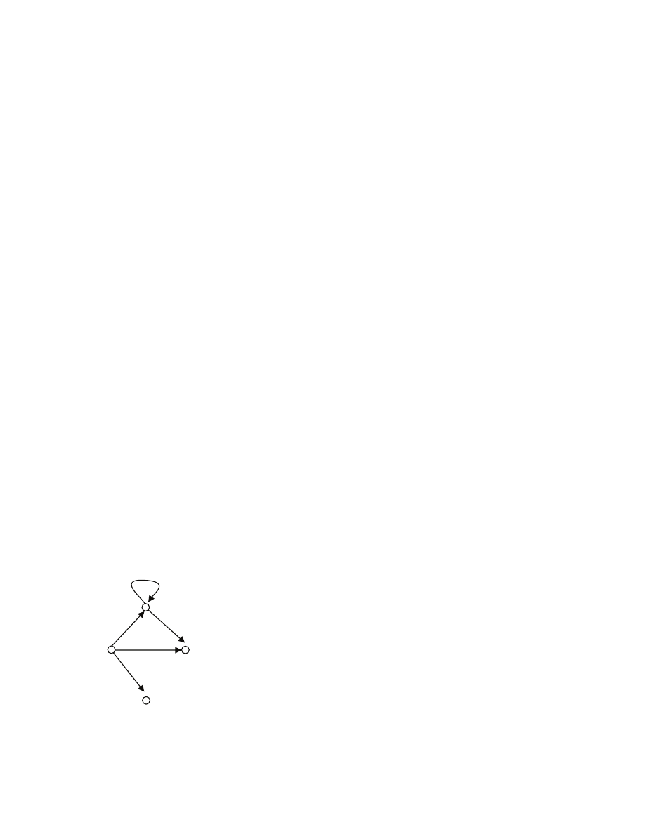
107
Fill-in-Tables(G,s)
1 OPT[s,0]
← 0
2 P[s,0]
← s
3 for all u≠s
4 OPT[u,0] ← ∞
5 P[u,0] ← “no path”
6 for
i=1,2,3,…
7 for all u
8 OPT[u,i] ← OPT[u,i-1]
9 P[u,i] ← P[u,i-1]
10 let B(u) = {w: there is an edge wÆu}
11 for all w∈B(u)
12 if OPT[w,i-1] + c
w
Æ
u
< OPT[u,i]
13 OPT[u,i] ← OPT[w,i-1] + c
w
Æ
u
14 P[u,i] ← P[w,i-1],u
[[note that Fill-in-Tables(G,s) runs forever]]
Ideally, we would like to compute the distance from s to any node u. This could possibly be done by
looking at how the content of the table changes: OPT[u,0], OPT[u,1], OPT[u,2], … . The upper case is
easy to identify without looking at too many i.
Fact
If there is a path from s to u, then there is a path with at most |V|-1 edges
Proof
If a path has more edges, it must have a cycle, and we can remove the cycle and decrease the number of
edges on the path. We can repeat the removal until the resulting path from s to u has at most |V|-1 edges.
█
Hence the upper case occurs if, and only if, OPT[u,|V|-1] is plus infinity.
How can we distinguish the middle and the lower cases? The problem is that a negative cycle reachable
from s might cause the sequence to decrease very, very slowly, which may make it time consuming to
distinguish the middle and the lower cases.
Example
s
u
w
-1
1000
1000
2
v
-1

108
Here OPT[u,1] = 2, and remains 2 as long as OPT[u,2000], and only decreases in the next iteration
OPT[u,2001]=1.
We can mitigate the problem by finding distances but under a certain restriction. We will compute the
distance from s to any other node only when no negative cycle is reachable from s. When, however, a
negative cycle is reachable from s, we will report it, but we might not compute distances. [[Note that in
the previous example there is a negative cycle reachable from s, so our algorithm will not find distances;
however, distances exist: the distance from s to v is -1, to w is -
∞, and to u is -∞; so in a sense the
algorithm will not be perfect]]. We will accomplish the mitigation by modifying the algorithm Fill-
in-Tables(G,s). Let us first record certain properties of the algorithm.
Fact (Stabilization)
If there is k such that during an iteration i=k, for every node u, the value of OPT[u,i] = OPT[u,i-1], then
for every subsequent iteration i
≥k, and every node u, OPT[u,i]=OPT[u,i-1].
█
Observation 1
If there is a path originating at s that includes a negative length cycle, then there is u such that OPT[u,|V|-
1] > OPT[u,|V|].
Proof
Let P be a path from s to w that has a negative length cycle. Hence the distance from s to w is minus
infinity. Suppose, by way of contradiction, that OPT[u,|V|-1]
≤ OPT[u,|V|] for all u. But OPT[u,|V|-
1]
≥OPT[u,|V], and so OPT[u,|V|-1] = OPT[u,|V|] for all u. Then the stabilization fact implies that
OPT[w,j] stays unchanged for any j
≥ |V|-1, a contradiction. But this leads to a contradiction, because
OPT[w,j] must tend to minus infinity when j tends to infinity.
█
Observation 2
If there is u such that OPT[u,|V|-1] > OPT[u,|V|], then there is a path originating at s that includes a
negative length cycle.
Proof
Let P be any shortest path from s to u with at most |V| edges. That path must actually have exactly |V|
edges, since if it has fewer edges, then it is a path with at most |V|-1 edges, and so OPT[u,|V|-1]
≤
OPT[u,|V|]. But then P has enough nodes to contain a cycle. Can this cycle be non-negative (i.e., “
≥0”)?
Suppose that the cycle is non-negative. But then removing the cycle does not increase the length, and
results in a path from s to u with at most |V|-1 edges. This would mean that OPT[n,|V|-1]
≤ OPT[u,|V|].
Hence the cycle must be negative.
█
[[Note that the proof of Observation 2 shows how to find a negative length cycle; we just need to inspect
the path P[u,|V|] and find a node that occurs on the path twice.]]
Bellman-Ford(G,s)
1
run Fill-in-Tables(G,s) for a finite number |V| of iterations
2
if for all u, OPT[u,|V|-1] = OPT[u,|V|] then
3
print “distance from s to u is “ OPT[u,|V|] “ and a shortest path is “ P[u,|V|]
4
else
5
print “negative cycle is reachable from s“

109
Theorem
The Bellman-Ford algorithm computes the distance from s to any node and a shortest path to that node,
whenever there is no negative cycle reachable from s.
Proof
Follows from the earlier observations.
“<=”
If there is no negative cycle reachable from s, then by Observation 2 OPT[u,|V|-1] = OPT[u,|V|], for all u,
and so the algorithm outputs OPT[u,|V|] and P[u,|V|] claiming that these are distances and shortest paths.
But then by the Stabilization Fact, the OPT stays unchanged beyond |V|-1. Hence the lower case cannot
happen, and OPT[u,|V|] properly determines the distance from s to u, and P[u,|V|] a shortest path when
OPT[u,|V|]<
∞.
“=>”
Suppose that there is a negative length cycle reachable from s. Then by Observation 1, there is u such that
OPT[u,|V|-1]>OPT[u,|V|], and so the algorithm reports that a negative cycle exists.
█
Implementation details
We can save on memory. Note that in any iteration i, we only need OPT[*,i-1] and OPT[*,i], so we do not
need to maintain OPT[*,0] , … , OPT[*,i-2]. We can represent P[u] more efficiently, just by keeping the
node directly before u on the path. So the total memory consumption will be O(|V|). The pointer
representation save us copying P[w,i-1] to P[u,i], which is a saving because P[w,i-1] may have many
nodes.
Theorem
The Bellman-Ford algorithm can be implemented to run in O(|V|
2
+|V|
⋅|E|) time and O(|V|) space.
Proof
The for loop makes |V| iterations. Each iteration takes O(|V|+|E|) time, just because, we are computing
minimum for every node v, and when computing the minimum we range w across B(v); we are thus
inspecting each edge once and each node once in the iteration, so the aggregate time of the iteration is
indeed O(|E|+|V|).
█
Extensions
We mitigated the problem of possibly large number of iterations of Fill-in-Tables(G,s) by not
reporting distances whenever a negative cycle is reachable, even though the distances exist then, only that
some are minus infinite. Here is how we can report distances even in this case. Start with G, and as long as
there is a negative cycle reachable from s, remove all the nodes of the cycle from G [[this may disconnect
the graph]]. After zero or more cycle removals, the remnant graph G’ has no negative cycle reachable
from s. Let U be all the nodes that have been removed [[s could be in U]]. Run Bellman-Ford on G’ to
compute distances and paths. Then go back to G, and for every u
∈U, compute the nodes in G reachable
from u. Set the distance from s for these nodes to minus infinity. This extension is correct: for any node v
of G, if there is a path to v that passes through a node of any of negative length cycle, then the distance
from s to v is minus infinity [[and v will be reachable from one of the removed cycles]], while if no path
to v passes through a negative length cycle, then the distance from s to v is just as it is in G’.
Wyszukiwarka
Podobne podstrony:
cis581 lecture notes chapter6
Pillay Lecture notes on Model theory (2002)
Corporate Identity Image and Brands lecture notes
2006 cis581 lecture notes
FM1 lecture notes v8
2006 581 pjwstk lecture notes
Lecture Notes in Statistics WEN37OYN77NFAXIV6BCPXJIW7VRMAHHHJIGYWUQ
Freitag Several complex variables local theory (lecture notes, web draft, 2001)(74s) MCc
Fred Kaps Lecture Notes
Rajeev S G Advanced classical mechanics chaos (Rochester lecture notes, web draft, 2002)(100s) PCtm
McCluskey A , McMaster B Topology Course Lecture Notes
Norbury General relativity and cosmology for undergraduates (Wisconsin lecture notes, 1997)(116s)
Angelo Stagnaro European Mentalism Lecture Notes 2005
Terry Harris Lecture notes for impromptu
Angelo Stagnaro European Mentalism Lecture Notes 2005
więcej podobnych podstron