
PHY 411 Advanced Classical Mechanics
(Chaos)
U. of Rochester Spring 2002
S. G. Rajeev
March 4, 2002

Contents
ii

Preface to the Course
Introduction
Only simple, exceptional, mechanical systems admit an explicit solution in
terms of analytic functions. This course will be mainly about systems that
cannot be solved in this way so that approximation methods are necessary.
In recent times this field has acquired the name ‘Chaos theory’, which has
grown to include the study of all nonlinear systems. I will restrict myself
mostly to examples arising from classical physics. The first half of the course
will be accessible to undergraduates and experimentalists.
Pre-requisites
I will assume that all the students are familiar with Classical mechanics
at the level of PHY 235, our undergraduate course (i.e., at the level of the
book by Marion and Thornton.) Knowledge of differential equations and
analysis at the level of our math department sophomore level courses will
also be assumed.
Books
I recommend the books Mechanics, by Landau and Lifshitz and Mathe-
matical Methods of Classical Mechanics by V. I. Arnold as a general reference
although there is no required textbook for the course. The course will be
slightly more advanced than the first book but will not go as far as Arnold’s
book. The more adventurous students should study the papers by Siegel,
Kolmogorov, Arnold and Moser on invariant torii.
Homeworks,Exams and Grades
I will assign 2-3 homeworks every other week. Some will involve simple
numerical calculations. There will be no exams. The course will be graded
Pass-Fail.
Syllabus
•Newton’s equations of motion.
•The Lagrangian formalism; generalized co-ordinates.
iii

iv
PHY411 S. G. Rajeev
•Hamiltonian formalism; canonical transformations; Poisson brackets.
•Two body problem of Celestial mechanics. Integrability of the equations
of motion.
•Perturbation theory; application to the three body problem.
•Restricted three body problem; Lagrange points.
•Normal co-ordinates; Birkhoff’s expansion; small denominators and reso-
nances.
•Invariant torii; Kolmogorov-Arnold-Moser theorems.
•Finding roots of functions by iteration: topological dynamics; onset of
chaos by bifurcation.
Special Topics for Advanced Students
•Ergodic systems. Sinai billiard table; geodesics of a Riemann surface.
•Quantum Chaos: Gutzwiller’s trace formula.
•Chaos in number theory: zeros of the Riemann zeta function.
•Spectrum of random matrices.

Chapter 1
Introduction
•Physics is the oldest and most fundamental of all the sciences; mechanics is
the oldest and most fundamental branch of physics. All of physics is modelled
after mechanics.
•The historical roots of mechanics are in astronomy-the discovery of reguar-
ity in the motion of the planets, the sun and the moon by ancient astrologers
in every civilization is the beginning of mechanics.
•The first regularity to be noticed is periodicity- but often there are several
such periodic motions superposed on each other. The motion of the Sun has
at least three such periods: with a period of one day, one year and 25,000
years (precession of the equinoxes). We know now that the first of these
is due to the rotation of the Earth relative to an inertial reference frame,
the second is due to the revolution of the Earth and the last is due to the
precession of the Earth’s axis of rotations.
•The first deep idea was to regard all motion as the superposition of such
periodic motion- a form of harmonic analysis for quasi-periodic functions.
This gave a quite good
description
of the motion.
•The precision at around 500 AD is already quite astonishing. The
Aryab-
hatiyam
gives the ratio of the length of the day to the year to an accuracy of
better than one part in ten million; adopts the heliocentric view when con-
venient; gives the length of each month to four decimal places; even suggests
that the unequal lengths of the months is due to the orbit of the Earth being
elliptical rather than circular. There were similar parallel developments in
China, the Arab world and elsewhere at that time.
•Astronomy upto and including the time of Kepler was mixed in with Astrol-
ogy and many mystic beliefs formed the motivation for ancient astronomers.
1

2
PHY411 S. G. Rajeev
•Kepler marks the transition from this early period to the modern era. The
explanation of his three laws by Newtonian mechanics is the first deep result
of the modern scientific method.
•Mechanics as we think of it today is mainly the creation of one man:
Isaac Newton. The laws of mechanics whch he formulated by analogy with
the axioms of Euclidean geometry form the basis of mechanics to this day,
although the beginning of the last century saw two basic changes to the
fundamental laws of physics.
•These are the theory of relativity and quantum mechanics. We still do not
have a theory that combines these into a single unified science. In any case
we will largely ignore these developments in these lectures.

Chapter 2
The Kepler Problem
•Much of mechanics was developed in order to understand the motion of
planets. Long before Copernicus, many astronomers knew that the appar-
ently erratic motion of the planets can be simply explained as circular motion
around the Sun. For example, the
Aryabhateeyam
written in 499 AD gives
many calculations based on this model. But various religious taboos and su-
perstitions prevented this simple picture from being universally accepted. It
is ironic that the same superstitions (e.g., astrology) were the prime cultural
motivation for studying planetary motion.
•Kepler used Tycho Brahe’s accurate measurements of planetary positions
to find a set of important refinements of the heliocentric model. The three
laws of planetary motion he discovered started the scientific revolution which
is still continuing.
1 The first law of Kepler is:
Planets move along elliptical orbits with the Sun
at a focus
.
2 An
ellipse
is a curve on the plane defined by the equation, in polar co-ordinates
(r, θ)
ρ
r
= 1 + cos θ.
2.1 The parameter
must be between
0
and
1
and is called the
eccentricity
. It measures the deviation of an ellipse from a circle: if
= 0
the curve is a circle of radius
ρ
. In the opposite limit
→ 1
( keeping
ρ
3

4
PHY411 S. G. Rajeev
fixed) it approaches a parabola. The parameter
ρ > 0
measures the size of
the ellipse.
•A more geometrical description of the ellipse is this: Choose a pair of points
on the plane
F
1
, F
2
, the
Focii
. If we let a point move on the plane such
that the sum of its distances to
F
1
and
F
2
is a constant, it will trace out
an ellipse.
•Derive the equation for the ellipse above from this geometrical description.
( Choose the origin of the polar co-ordinate system to be
F
2
). What is the
position of the other focus
F
1
?
•The line connecting the two farthest points on an ellipse is called its
major
axis
; this axis passes through the focii. The perpendicular bisector to the
major axis is the
minor axis
. If these are equal in length, the ellipse is a
circle; in this case the focii coincide. The length of the major axis is called
2a
usually. Similarly, the semi-minor-axis is called
b
.
•Show that the major axis is
2ρ
1
−
2
and that the eccentricity is
=
√
h
1
−
b
2
a
2
i
.
•The eccentricity of planetary orbits is quite small: a few percent. Comets
and some asteroids and planetary probes have very eccentric orbits.
•If the eccentricity is greater then one, the equation describes a curve that
is not closed, called a
hyperbola
.
•The second law of Kepler concerns the angular velocity of the planet:
3
The line connecting the planet to the Sun sweeps equal areas in equal times
.
3.1 Since the rate of change of this area is
1
2
r
2 dθ
dt
, this is the statement
that
1
2
r
2
dθ
dt
= constant.
•The third law of Kepler gives a relation between the size of the orbit and
its period.
4
The ratio of the cube of the semi-major axis to the square of the period is
the same for all planets
.

PHY411 S. G. Rajeev
5
•Newton’s derivation of these laws from the laws of mechanics was the first
triumph of modern science.
5 In the approximation in which the orbits are circular, Kepler’s laws imply the
force on a planet varies inversely as the square of the distance from the Sun.
5.1 The eccentricities are small ( a few percent); so this is a good approxi-
mation. The first law then states that the orbits are circular with the Sun at
the center; the second that the angular velocity is a constant. This constant
is
˙
θ =
2π
T
, where
T
is the period. So the acceleration of the planet is
pointed towards the Sun and has magnitude
r ˙
θ
2
= 4π
2 r
T
2
. The third law
says in this approximation that
r
3
T
2
= K
, the same constant for all planets.
Thus the acceleration of a planet at distance
r
is
K
4π
2
1
r
2
. Thus the force on
a planet must be proportional to its mass and inversely proportional to the
square of its distance from the Sun.
•Extrapolating from this Newton arrived at the Universal Law of Gravity:
6 The gravitational force on a body due to another is pointed along the line
connecting the bodies; it has magnitude proportional to the product of masses
and inversely to the square of the distance.
6.1 If the positions are
r
1
, r
2
and masses
m
1
, m
2
, the forces are respec-
tively
F
1
=
d
[r
2
− r
1
]
Gm
1
m
2
|r
1
− r
2
|
,
F
2
=
d
[r
1
− r
2
]
Gm
1
m
2
|r
2
− r
1
|
7 Newton’s second law gives the equations of motion of the two bodies:
m
1
d
2
r
1
dt
2
= F
1
,
m
2
d
2
r
2
dt
2
= F
2
.
8 The key to solving the equations of motion is the set of conserved quantities.

6
PHY411 S. G. Rajeev
9 Since
F
1
+ F
2
= 0
for any isolated system ( Newton’s third law) the total
momentum is always conserved:
m
1
dr
1
dt
+ m
2
dr
2
dt
= P,
dP
dt
= 0.
10 We can change variables from
r
1
, r
2
to the
center of mass
and
relative
co-ordinates:
R =
m
1
r
1
+m
2
r
2
m
1
+m
2
, r = r
2
− r
1
to get
d
2
R
dt
2
= 0,
m
d
2
r
dt
2
=
−ˆr
Gm
1
m
2
|r|
2
where
m =
m
1
m
2
m
1
+m
2
is the
reduced mass
.
10.1 The first equation is trivial; the second is the same as that of a single
body at position
r
moving in a central force field: we have reduced the two
body problem to the one body problem.
11 A
central force field
is pointed along the radial vector and has magnitude
depending only on the radial distance. Angular momentum
L = mr
×
dr
dt
is
conserved in any central force field.
12 Hence the vector
r
always lies in the constant plane orthogonal to
L
.
13 In plane polar co-ordinates, the angular momentum is
L = mr
2
dθ
dt
.
14 We have jsut derived Kepler’s second law: since
m
is a constant, conser-
vation of angular momentum implies that the areal velocity
1
2
r
2 dθ
dt
is a constant.
15 A central force field is
conservative
: it is the gradient of a scalar function:
F =
−∇U
where
U
is a function only of the radial distance.
15.1 For the gravitational force,
U (r) =
−
Gm
1
m
2
r
2
.

PHY411 S. G. Rajeev
7
16 In any conservative force field, the total energy is conserved:
1
2
m
h
˙r
2
+ r
2
˙
θ
2
i
+ U (r) = E.
17 To determine the shape of the orbit we need
r
as a fucntion of
θ
. We can
eliminate
t
in favor of
θ
in teh above equation using conservation of angular
momentum:
dθ
dt
=
L
mr
2
⇒
dr
dt
=
dr
dθ
L
mr
2
=
−
L
m
du
dθ
where
u =
1
r
.
18 Thus we get
L
2
2m
[u
02
+ u
2
] = E
− U(u), ⇒ θ − θ
0
=
Z
u
u
0
2m
L
2
[E
− U(w)] − w
2
−
1
2
dw
19 Exercise: Solve this ODE and obtain the equation for the ellipse for the case
of the Kepler problem.
20 The rate of change of area is a constant,
˙
A =
1
2
r
2
˙
θ =
L
2m
; the total area
of the ellipse is
A = πab
. These two facts combine to give us the period of the
motion,
T =
A
˙
A
.
21 Exercise: Derive Kepler’s third law by simplifying the expression for the
period.

Chapter 3
The Action
•Newton formulated mechanics in terms of differential equations. Even at
that time there was a parallel view (eg., Leibnitz) that the laws of mechanics
could be formulated as a variational principle.
•For example the position of a body of in stable equilibrium is the minimum
of potential energy. More generally any extremum of the potential is an
equilibrium.
Is there a similar principle which determines the path of a
particle in motion?
•Let
Q
be the space of all instantaneous positions of the system. For a
point particle it is the Euclidean space
R
3
; for a system of
n
particles it
is
R
3n
; for a pendulum of length
L
it is
S
1
, the circle of radius
L
. This
space is called the
configuration space.
•The path is described by a map from the real line (the set of values of
time
) to the configuration space. This curve must be differentiable so that
we can speak of velocities: so the configuration space must be a differentiable
manifold and the curve must be differentiable.
•The
dimension
of the configuration space is the number of real numbers
we must specify to fix the position of the particle at any instant. It is also
called the
number of degrees of freedom
.
•Given the initial time, initial position and the final time and final position,
we expect a unique curve to connect them that satisfies the laws of motion.
This is reasonable if these laws are second order differential equations.
•Among all curves with prescribed endpoints, the curve that satisfies the
laws of motion are the extrema of a quantity called the
action
.
8

PHY411 S. G. Rajeev
9
•This action is the integral of a function of the position, velocity and time:
S[q] =
Z
t
2
t
1
L(q, ˙
q, t)dt
If we vary
q
slightly
q
→ q + δq
δS =
Z
"
δq
i
∂L
∂q
i
− δ ˙q
i
∂L
∂ ˙
q
i
#
dt
•The variation must vanish at the endpoints:
δq
i
(t
1
) = 0 = δq
i
(t
1
)
. This
gives (after an integration by parts)
∂L
∂q
i
−
d
dt
∂L
∂ ˙
q
i
= 0.
These differential equations are called the
Euler-Lagrange
equations.
•
Example
: Free particle. For a free particle in
R
3
, all points are the same,
and all directions are the same and all instants of time are the same. These
imply that the Lagrangian is independent of the Cartesian co-ordinates
q
i
, and of time
t
. It is a function only of
˙q
2
. Galelean invaraince implies
in fact that it is proportional to tehe square of the velocity:
1
2
m ˙q
2
. The
constant
m
is the
mass
.
•A basic principle of mechanics is that the motion of a system reduce to that
of a free particle for short enough time intervals. We can interpret this to
mean that the equations of motion are second order quasi-linear differential
equations (quasilinear means linear in the velocities: all the nonlinearities
are in the coordinates). The Lagrangian for a wide class of systems is of the
form
L(q, ˙
q, t) =
1
2
g
ij
(q, t) ˙
q
i
˙
q
j
+ A
i
(q, t) ˙
q
i
− V (q, t)
where
g
ij
is a positive symmetric tensor.
•The simple example of a particle moving in
R
3
in the presence of a
potential has
L(q, ˙
q, t) =
1
2
m ˙
q
i
˙
q
i
− V (q, t)

Chapter 4
Symmetry and Conservation
Laws
•It is not possible to improve on the discussion in the book by Landau and
Lifshitz, so I just refer you to it.
10

Chapter 5
Systems with one degree of
Freedom
•Consider a system with one degree of freedom with Lagrangian
L =
1
2
m ˙x
2
− V (x).
Any conservative system with one degree of freedom can be brought to this
form by a choice of co-ordinates. For example the more general Lagrangian
L =
1
2
g(q) ˙
q
2
− U(q).
can be brought to our form by the change of variables
x(q) =
Z
q
q
0
√
g(q)dq,
V (x) = U (q(x)).
•The equations of motion can be integrated once to get a first order ODE.
The simplest way to understand this is to not that the total energy is con-
served:
1
2
˙x
2
+ V (x) = E
Thus we can reduce the solution of the equation to quadrature:
t(x)
− t
0
=
√
2
Z
x
x
0
dx
√
[E
− V (x)]
.
11

12
PHY411 S. G. Rajeev
Inverting this function gives position as a function of time.
•
Exercise
For the simple harmonic oscillator:
V (x) =
1
2
ωx
2
,
so that
t(x)
− t
0
=
√
2
Z
x
x
0
dx
√
[E
−
1
2
ωx
2
]
.
Evaluate the integral by trigonometric substitutions.
•The
simple pendulum
is a ball of mass
m
hung from a fixed point by a
rigid rod of length
l
. The Lagrangian is
L =
1
2
ml
2
˙
θ
2
+ mgl cos θ.
Conservation of energy gives
1
2
ml
2
˙
θ
2
− mgl cos θ = E.
The energy thus has minimum value
−mgl
when the ball is at rest at
θ = 0
. If
E < mgl
the ball will oscillate back and forth; when
E > mgl
the
ball will rotate around the point of support.
•The integral above will give the answer for time as a function of angle
in terms of an
elliptic integral
. There are many excellent books on elliptic
integrals eg.
Higher Transcendental Functions
ed. by Erdelyi. We will
look instead at the angle as a function of time which involve single functions
called
elliptic functions
.
•The Jacobi elliptic functions
sn (u, k), cn (u, k), dn (u, k)
are single
valued meromorphic functions of two complex variables
u
and k. They are
generalizations of the trigonometric functions. They can be defined by the
system of differential equations
d sn (u, k)
du
= cn (u, k) dn (u, k),
d cn (u, k)
du
=
− sn (u, k) dn (u, k)
d dn (u, k)
du
=
−k
2
sn (u, k) cn (u, k).

PHY411 S. G. Rajeev
13
with the boundary conditions
sn (0, k) = 0, cn (0, k) = 1, dn (0, k) = 1.
•It follows that (writing
s
for
c
for
cn
etc.)
s
2
+ c
2
= 1,
k
2
s
2
+ d
2
= 1,
d
2
− k
2
c
2
= 1
− k
2
for all
(u, k)
(they are like conservation laws for the ODE). (Prove this by
explicit differentiation!) The differential equation can thus be written as
s
02
= (1
− s
2
)(1
− k
2
s
2
).
•From the symmetry of the equation and boundary condition under reflec-
tion
u
→ −u
, we see also that
sn (
−u, k) = − sn (u, k), cn (−u, k) =
cn (u, k), dn (
−u, k) = dn (u, k)
.
•Clearly when
k = 0
the solution is
sn (u, 0) = sin u
,
cn (u, 0) = cos u
and
dn (u, 0) = 1
. These are the limiting values of the Jacobi functions.
•The differential equation for the angle of the pendulum can be solved in
terms of
sn
by some change of variables. Once we notice the similarity
between the two equations, we put in the ansatz
u = ωt, sin
1
2
θ(t) = A sn (u, k).
With these definitions the ODE for the pendulum reduces to
2ml
2
ω
2
A
2
"
d sn (u, k)
du
#
2
= [E + mgl
− 2mglA
2
sn
2
(u, k)][1
− A
2
sn
2
(u, k)]
•Comparing with the ODE for
sn
we get
E + mgl = 2mglA
2
= 2ml
2
A
2
ω
2
, A = k
as one way to reduce our ODE to Jacobi’s. (There are is another which
corresponds to a symmetry of
sn (u, k)
under
k
→
1
k
.)
•We get
ω =
g
l
1
2
,
k
2
=
E + mgl
2mgl
.

14
PHY411 S. G. Rajeev
The solution is thus
sin
1
2
θ(t) = k sn (ω(t
− t
0
), k).
•In the limit
E
→ −mgl
,we get
k
→ 0
, so that the solution reduces to
small oscillations around the point
θ = 0
θ(t)
∼ 2k sin(ω(t − t
0
))
This is a familiar result . Indeed we recognize
ω
as the angular frequency
of this simple harmonic motion.
•When
E < mgl
we expect oscillatory motion around the equilibrium
point: there isnt enough energy to go all the way around. Thus physically
we expect
sn (u, k)
to be a periodic function. We can even get a formula
for the period from the earlier formula for time as a function of position: it
is just four times the time it takes to go from
θ = 0
to the maximum value
of the angle, which is the root of
E + mgl cos θ = 0
. The period can be
expressed in terms of the
complete elliptic integral
K(k) =
Z
π
2
0
dφ
√
[1
− k
2
sin
2
φ]
.
In fact,
sn (u + 4K(k), k) = sn (u, k).
•We can analytically continue the function to the complex plane in the
u
variable. Surprsingly,
sn
is also periodic with an imaginary period: it is a
doubly periodic function
of
u
. There is a simple physical way to understand
this. Replacing
t
→ it
in the equation of motion amonts to reversing the
sign of the potential and of energy. Thus in imaginary time we get the same
problem! Changing
E
→ −E
is the same as
k
→
√
[1
− k
2
]
. So we have
a formula for the other period:
sn (u + 4iK
0
(k), k) = sn (u, k)
with
K
0
(k) = K(
√
[1
− k
2
]).

PHY411 S. G. Rajeev
15
(Here the prime does
not
stand for the derivative.)
•Since
sn (0, k) = 0
we see that it has an infinite number if zeros, at the
points of a lattice in the complex plane. A doubly periodic analytic function
must have some singularities: otherwise it would be constant by Lioville’s
theorem.
sn (u, k)
has simple poles on a lattice as well.
•
Exercise
Show that
sn (u, 1) = tanh u
. What kind of motion of the
pendulum does this correspond to?. Show that as
E
→ ∞
the motion
reduces to uniform circular motion with a large frequency.
•
Exercise
Use the differential equation to relate
sn (u,
1
k
)
to
sn (u, k)
.
Show then that as
E
→ ∞
the solution tends to uniform circular motion.
•There is much more to the story; but you have to study the rest of this
fascinating story from other books. I recommend the book
Elliptic Functions
by K. Chandrashekaran.

Chapter 6
Nonlinear Oscillations in One
Dimension
22 An oscillation whose amplitude is not infinitesimal is described by a nonlinear
equation.
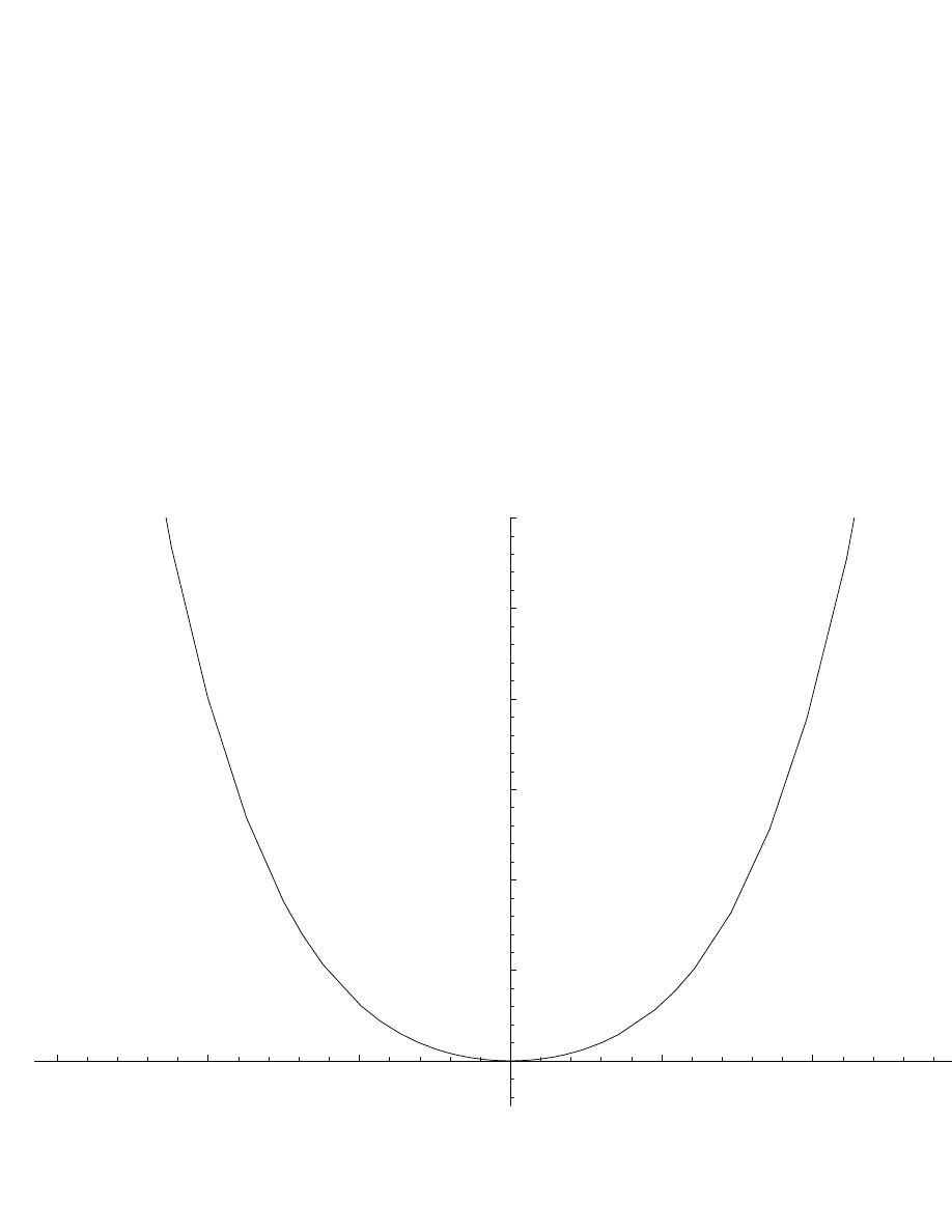
23 The simplest case is a one dimensional system with a potential that has a
unique extremum, which is a minimum (one stable equilibrium).
23.1 For example,
V (x) =
1
2
kx
2
+ λx
4
with
k, λ > 0
has a unique
minimum at the origin.
23.2 Qualitatively such oscillations are similar to the harmonic oscillator:
all orbits are periodic. The main difference is that the period might depend
on the energy ( which is a measure of how much the oscillation departs from
the equilibrium.)
23.3 The Lagrangian
L =
1
2
m ˙x
2
− V (x)
leads to the equation of motion
m¨
x =
−V
0
(x).
16

PHY411 S. G. Rajeev
17
23.4 It is often convenient to regard the equations as a pair of first order
equations for position and momentum
dx
dt
=
p
m
,
dp
dt
=
−V
0
(x).
23.5 Given the value of the position and momentum at any time, these
equations determine them for all future times. There are many reliable nu-
merical methods (for example, the Runge–Kutta method, built into Mathe-
matica) that compute this solution with sufficient accuracy.
23.6 Thus, it is convenient to regard the solution as a curve in the plane
(x, p)
; if we give initial conditions ( where the system is at any given time as
a point in this plane) the equations determine where it will be for all future
times.
24 The motion of a conservative system is described as a curve in the
phase
space
; each point in phase space is a set of values of position and momentum.
24.1 In our case of oscillations in one position variable, the phase space is
two dimensional.
25 In the case of a system of one degree of freedom, the conservation of energy
determines the shape of these curves.
25.1 The energy expressed as a function of position and momenta is called
the
hamitonian
:
H(x, p) =
p
2
2m
+ V (x);
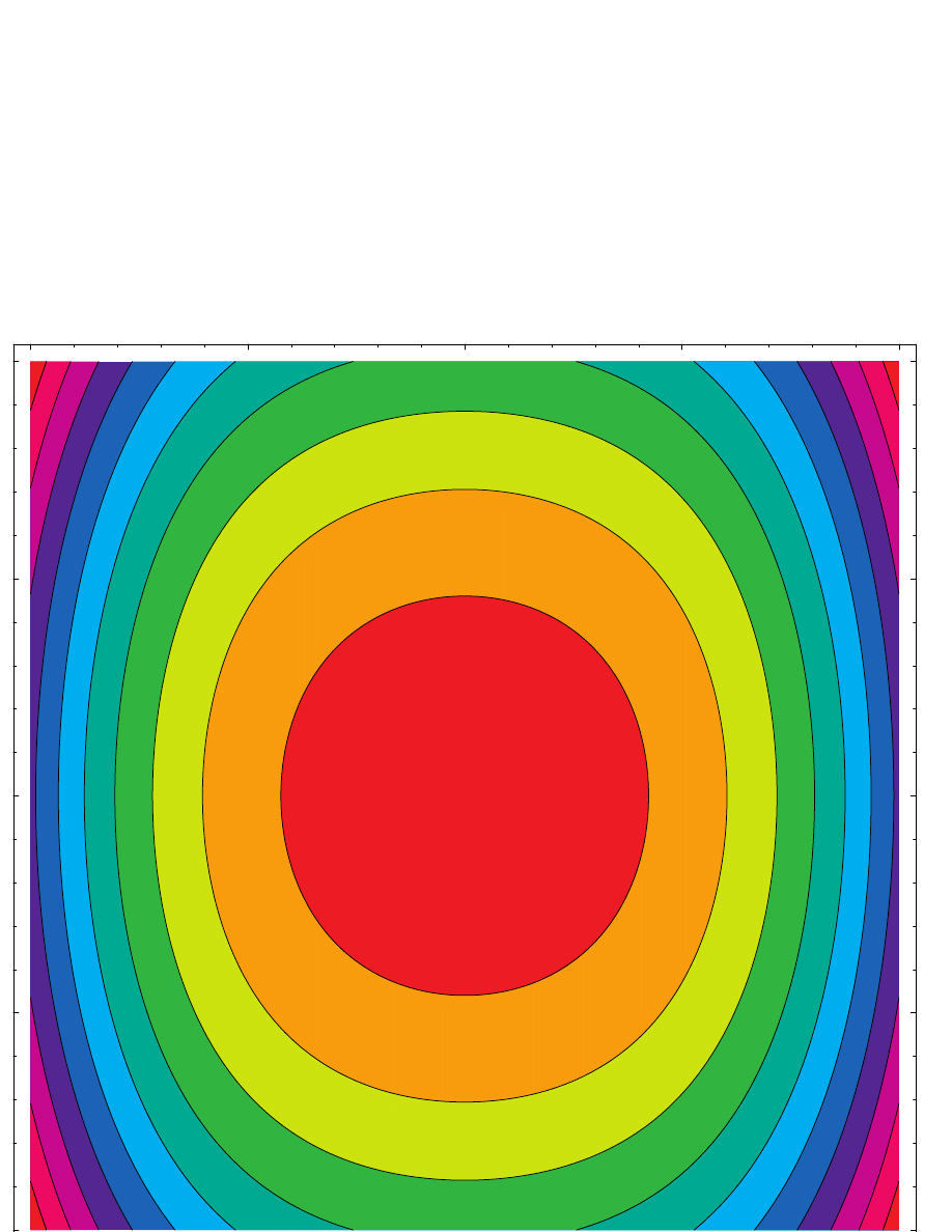
We can imagine the hamiltonian as a function on the plane
(x, p)
, plotted
as a sort of ‘hill’. The bottom of the valleys of this plot describe stable
equilibrium points. The system evolves along contour plots,i.e., curves along
which the energy is a constant.
25.2 If
V (x)
has a single stable equilibrium point, these curve are ellipses
for small values of energy; as energy grows they will still be closed curves,
but no longer ellipses.
18
PHY411 S. G. Rajeev
-1.5
-1
-0.5
0.5
1
1.5
0.5
1
1.5
2
2.5
3
PHY411 S. G. Rajeev
19
-1
-0.5
0
0.5
1
-1
-0.5
0
0.5
1

20
PHY411 S. G. Rajeev
25.3 The period of the orbit is
T (E) = 2
√
2
m
Z
x
2
(E)
x
1
(E)
dx
√
[E
− V (x)]
where
x
1
(E), x
2
(E)
are solutions of the equations
V (x) = E
. (They are
called
turning points
). In this case there will be exactly two solutions, as
long as the energy is greater than the minimum value. The system oscillates
between these two points.
25.4 As we approach the minimum value of energy the turning points ap-
proach merge with each other and we get a static solution.
26 The area enclosed by the curve of constant energy
W (E)
, has many
interesting properties; for example the period of the orbit is
T (E) =
dW (E)
dE
.
26.1 Prove this!.
26.2 Thus the area of an orbit is a monotonically increasing function of the
energy.
27 In the semiclassical approximation of quantum mechanics, the energy levels
are given by the
Bohr-Sommerfeld
condition:
W (E) = n¯
h, n = 0, 1, 2,
· · ·
27.1 The number of energy levels of energy less than
E
is the area enclosed
by the curve
H(x, p) = E
in units of Plank’s constant.
28 Thus the density of energy levels at energy
E
is equal to the classical
period divided by Plank’s constant:
T (E)
¯
h
.
PHY411 S. G. Rajeev
21
-1.5
-1
-0.5
0.5
1
1.5
0.5
1
1.5
2
2.5
3
22
PHY411 S. G. Rajeev
-1
-0.5
0
0.5
1
-1
-0.5
0
0.5
1

PHY411 S. G. Rajeev
23
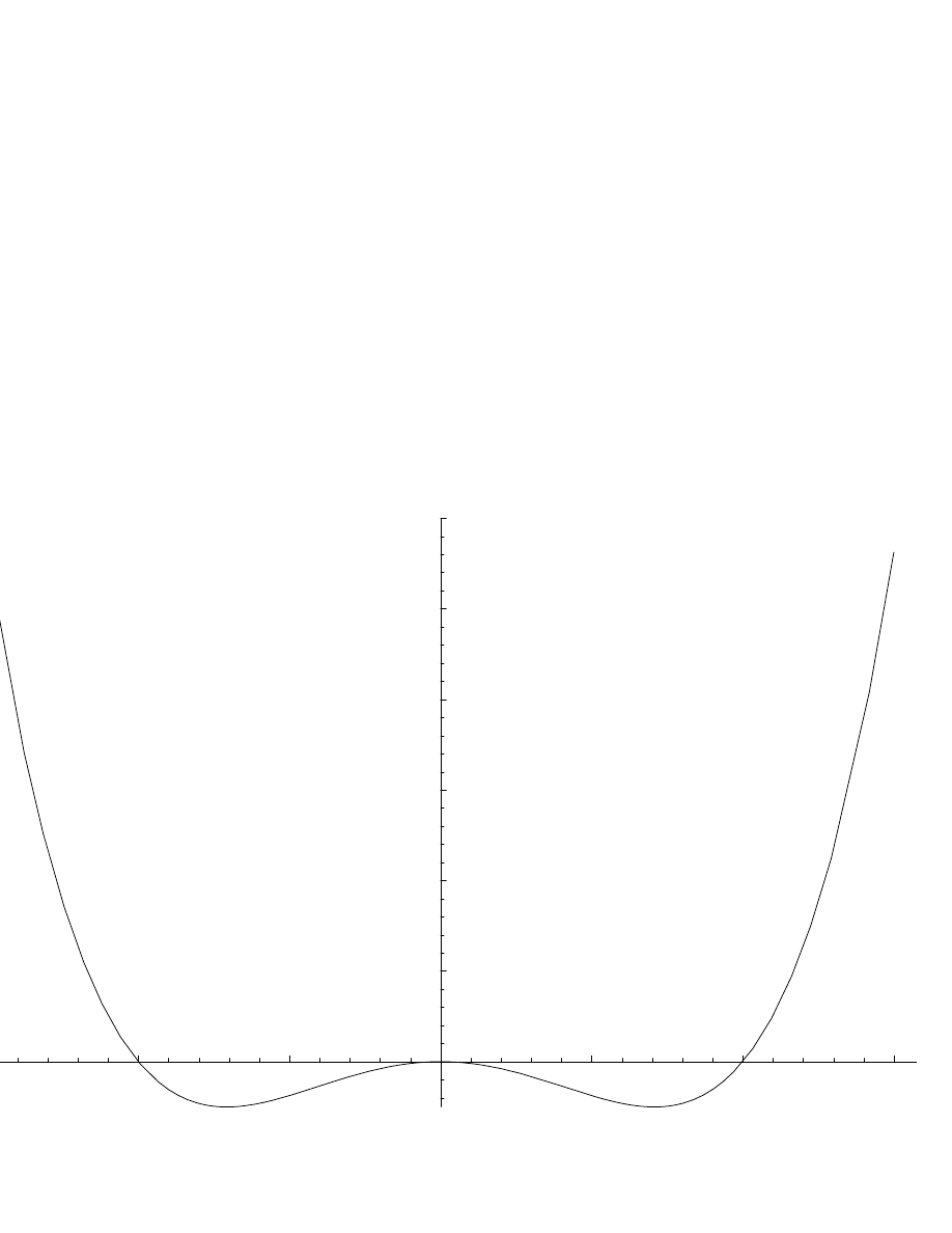
29 Now consider the case where
V (x)
has two stable equilibrium points.
29.1 If there are two stable equilibrium points, there must be one unstable
equilibrium in between them. ( Prove this!).
29.2 Let us (for simplicity) assume that the potential is an even function:
V (x) = V (
−x)
; so that the two stable points are symmetrically placed
around the origin, and the origin itself is an unstable equilibrium point.
29.3 Exercise: Generalize the analysis below to the case where
V (x)
is
not symmetric.
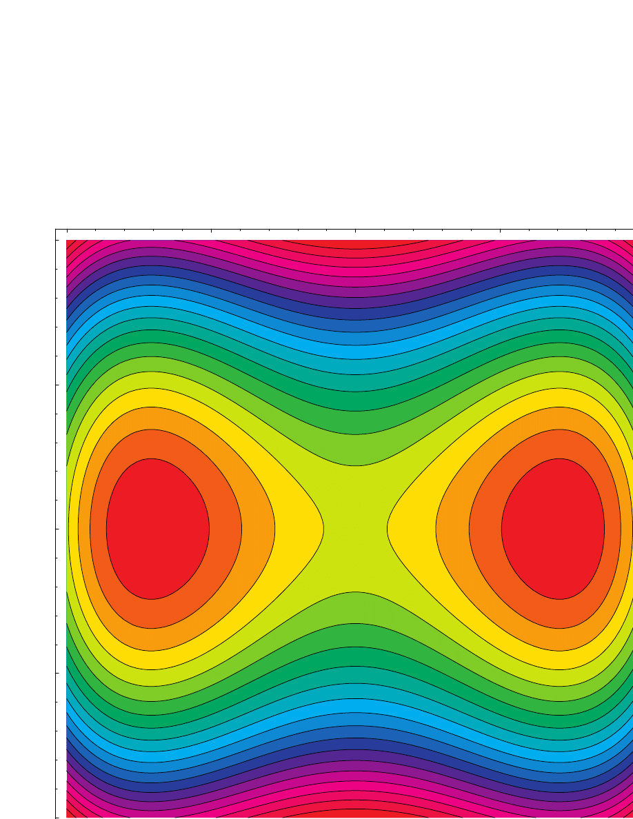
29.4 With two stable equilibria, the orbits for small energy will be approx-
imately ellipses around each stable equilibrium point: the set of points with
a given value of energy is
disconnected
. For large energy they will be curves
that surround both stable equilibria: it is a connected curve.
29.5 Let
E
min
be the minimum of the potential, and
E
cr
its value at
the unstable equilibrium point . For
E
min
< E < E
cr
, there are four real
solutions to the equation
V (x) = E
,
x
1
(E) < x
2
(E) < 0 < x
3
(E) < x
4
(E)
. The system oscillates between either
x
1
(E)
and
x
2
(E)
or between
x
3
(E)
and
x
4
(E)
; it never reaches the unstable equilibrium point at the origin.
29.6 As
E
→ E
cr
, the two middle turning points
x
3
(E)
and
x
4
(E)
approach each other and eventually dissappear (i.e., become complex); for
E > E
cr
, there are only two real solutions
x
1
(E), x
4
(E)
for the equation
V (x) = E
. The system oscillates between these two points, which means it
passes through all three equilibrium points.
29.7 Thus at the
critical
value of energy
E
cr
the nature of the orbits
change drastically. If the system starts out at this point with an infinites-
imally small but small postive value of energy it will fall into the positive
minimum and return to the original point after a long time; with an in-
finitesimally small but negative momentum it will fall into the other stable
equilibrium point and return. The period of this motion is infinite ( we will
see this soon).
29.8 Thus we discover the significance of unstable equilibria: they describe
orbits that are the boundary between those that circle one of the equilibrium
points and those that surround both.These are called
critical orbits
.

24
PHY411 S. G. Rajeev
29.9 The critical orbit has infinite period; more precisely, the period
T (E)
diverges as
E
→ E
cr
. The nature of this divergence is independent of the
details of the potential. As long as the unstable equilibrium point is non-
degenerate, ( this means that
V
00
is non-zero there)
T (E)
∼ log |E − E
cr
|
as
E
→ E
cr
.
30 The area of orbits is a subtle quantity when
E
min
< E < E
cr
.
30.1 For, the curve encloses two separate ( disconnected) regions; the deriva-
tive of the are of each connected component is the period of that piece.
30.2 This function has a singularity at the critical values of energy: two
disconnected areas merge into one so that suddenly the area doubles. The
area of each piece will have a jump discontinuity, but the sum of the two
areas will change continuously.
30.3 But the derivative of even the sum of the areas will diverge logarith-
mically, as it is proportionalo the period of the critical orbit.
30.4 Thus the density of energy levels has spikes at critical values of the
energy . This fact has interesting consequences in the theory of metals, as the
conductivity of metals is proportional to the density of states at the Fermi
energy.
31 There are even further subtleties in quantum mechanics of double-well po-
tentials: the system can
tunnel
from one of the minima to the other.

Chapter 7
Scattering In One dimension
•Let
V (x) : R
→ R
be a potential on the real line such that
lim
|x|→∞
V (x) =
0
. A particle moves from
x =
−∞
with an initial energy
E
and it will
either be reflected back to
x =
−∞
(if it doesnt have enough energy to
overcome some ‘hilly’ part of the potential) or be transmitted to
x =
∞
.
Let us consider for simplicity the case
V (x)
≤ 0
so that all particles are
transmitted. Let us set the mass equal to
2
to avoid unpleasant constants.
•Conservation of energy gives
˙x
2
+ V (x) = E
From this we can calculate the time of transit from
x =
−L
to
x = L
:
T (E, L) =
Z
L
−L
dx
√
[E
− V (x)]
We can compare this to the time it would have taken in the absence of a
potential:
T
0
(E, L) =
Z
L
−L
dx
√
E
.
Each of these integrals diverge as
L
→ ∞
but there difference will converge
for potentials of finite range: the particle will take a little bit less time to
transit in the presence of a potential, as it is moving faster (when
V (x) < 0
). This time difference is
T (E) =
Z
∞
−∞
dx
n
[E
− V (x)]
−
1
2
− E
−
1
2
o
.
25

26
PHY411 S. G. Rajeev
This quantity is the classical analogue of the scattering phase shift in quan-
tum theory. ( Actually an even closer analogue is the difference in the action
between the two paths, which is exactly the classical limit of the scattering
phase shift).
•Often in physics we are interested in inverse problems. Is it possible to
reconstruct the potential
V (x)
knowing the time delay
T (E)
of scattering
for all energies? That is, can we solve the above integral equation for
V (x)
given
T (E)
?.
•This is a nonlinear integral equation which is hard to solve. But a little trick
will reduce it to a linear integral equation: we try to find the inverse function
of
V (x)
. That is we look for
x(V )
. But this is a multiple-valued function:
since
V (x)
goes from
0
at
x =
−∞
to a negative value to
0
again at
x =
∞
, its inverse is at least double valued. We can avoid this problem by
restricting ourselves to potentials that are symmetric
V (
−x) = V (x)
and
monotonic in the range
0 < x <
∞
. Then,
x(V )
will be single valued
function with range
0 < x(V ) <
∞
when
V
is in the range
V
0
< V < 0
.
(Here,
V
0
= V (0)
).
T (E) = 2
Z
0
V
0
dx(V )
dV
n
[E
− V ]
−
1
2
− E
−
1
2
o
dV.
which is a linear integral equation for
dx(V )
dV
. This can be solved using
the theory of
fractional integrals
. Thus in this case the potential can be
reconstructed from the scattering data.
•
Aside
The
fractional integral of order
µ
of a function
f (x)
is
R
µ
f (y) =
1
Γ(µ)
Z
y
0
f (x)(y
− x)
µ
−1
dx.
The path of integration in the complex
x
plane is the straight line connecting
the origin to
y
. It has the following properties (after appropriate analytic
continuations):
R
µ
R
ν
f = R
µ+ν
f,
R
1
f (y) =
Z
y
0
f (x)dx
R
µ
d
n
f
dx
n
= R
µ
−n
f.

PHY411 S. G. Rajeev
27
This means that
R
µ
f can be thought of as an analytic continuation of the
n
th derivative of
f
to a negative (or even complex) value
−α
.
•In particular,
g(y) =
1
Γ(µ)
Z
y
0
f (x)(y
− x)
µ
−1
dx
⇒ f(y) =
1
Γ(
−µ)
Z
y
0
g(x)(y
− x)
−µ−1
dx.
This is the idea behind solution of integral equations such as the ones above.

Chapter 8
Small Oscillations with Many
Degrees of Freedom
See Landau and Lifshitz Chapter 5.
•One of the simplest mechanical systems is the
simple harmonic oscillator
with Lagrangian
L =
1
2
m ˙x
2
−
1
2
kx
2
.
•The equations of motion
m¨
x + kx = 0
have the well known solutions in
terms of trigonometric functions:
x(t) = a cos[ω
0
(t
− t
0
)]
where the
angular frequency
ω
0
=
√
(k/m)
. The constants
a
and
t
0
are constants of integration. They have simple physical meanins:
A
is the
maximum displacement and
t
0
is a time at which
x(t)
has this maximum
value. The energy is conserved and has the value
1
2
ma
2
.
•Although the solutions
x(t)
are real for physical reasons, it turns out to
be convenient to think of them as the real parts of a complex solution:
x(t) = Re Ae
iω
0
t
.
Then
a =
|A|
and
t
0
=
−
arg A
ω
0
.
•
Example
Imagine a particle of mass
m
moving on a line atttched to two
fixed points
a, b
on either side, by springs of strengths
k
1
and
k
2
. What
is the angular frequency?
L =
1
2
˙x
2
−
1
2
k
1
(x
− a)
2
−
1
2
k
2
(x
− b)
2
28

PHY411 S. G. Rajeev
29
which is
L =
1
2
˙x
2
−
1
2
[k
1
+ k
2
]
"
x
−
k
1
a + k
2
b
k
1
+ k
2
!#
2
+ constant.
Thus we get simple harmonic oscillation around the point
k
1
a+k
2
b
k
1
+k
2
with
angular frequency
h
k
1
+k
2
m
i
1
2
.
•Now consider an external force
F (t)
acting on a simple harmonic oscillator:
m¨
x + kx = F (t).
This equation can be solved by the Fourier transform:
x(t) =
Z
˜
x(ω)e
iωt
dω
2π
,
F (t) =
Z
˜
F (ω)e
iωt
dω
2π
to get
m[ω
2
0
− ω
2
]˜
x(ω) = ˜
F (ω).
Thus a solution is
x(t) =
1
m
Z
˜
F (ω)
ω
2
0
− ω
2
dω
2π
.
But this integral is singular at two points along the real line: we need to
somehow modify the contour of integration to make the integral meaningful.
The choice of this rule will depend on two constants, which are determined
by the boundary conditions on the equation of motion.
•Let us now consider a more general mechanical system with Lagrangian
L =
1
2
X
ij
g
ij
(q) ˙
q
i
˙
q
j
− V (q).
Practically any mechanical system (except those with velocity dependent
forces) is of this form. The equation of motion is
d
dt
X
j
g
ij
(q) ˙
q
j
+
∂V
∂q
i
= 0.

30
PHY411 S. G. Rajeev
Any point at which
∂V
∂q
i
= 0
is an
equilibrium point
: there is a constant
solution to the equation of motion at that point.
•We will now study the system in the infinitesimal neighborhood of an
equilibrium point. We can choose choose co-ordinates so that this point is
at the origin.
L =
1
2
g
ij
˙
q
i
˙
q
j
−
1
2
K
ij
q
i
q
j
− V (0) + O(q
3
).
Here
K
ij
=
∂
2
V
∂q
i
∂q
j
(0)
is the matrix of second derivatives of the potential:
also called the
Hessian
.
•The first thing to note is that
stable equilibrium points correspond to
minima of the potential
; i.e.,
K
must be positive. An equilibrium point is
stable if the linearized equations of motion have bounded solutions for any
initial condition. Now we get the equation of motion (using matrix notation)
X
j
g
ij
d
2
q
j
dt
2
+
X
j
K
ij
q
j
= 0.
We can look for solutions of the form
q
j
= A
j
e
iωt
. The solution is bounded
if the frequency is real. Thus for a stable equilibrium point all the frequencies
must be real. We get the eigenvalue problem:
X
j
[
−ω
2
g
ij
+ K
ij
]A
j
= 0.
•No we already know that
g
ij
is a positive: otherwise kinetic energy would
not be a positive function of the velocities. Thus we can regard it as defining
an inner product on the
n
-dimensional real vector space. Thus we can
choose a co-ordinate system in which
g
ij
= 0
for
i
6= j
and
g
ij
= 1
for
i = j
. There is a procedure (Gramm-Schmidt orthogonalization) that
even constructs this orthonormal co-ordinate system explicitly. Then we get
a more familiar eigenvalue problem
KA = ω
2
A.
We still have some freedom in the co-ordinate system: transformations that
are orthogonal with respect to the inner product
g
will map orthonormal
systems to each other. A symmetric matrix such as
K
can be diagonalized

PHY411 S. G. Rajeev
31
using such a transformation and the diagonal entries are then the eigenvalues.
Now in order that ω
be real, the eignvalues of
K
should be positive: it
must be a positive matrix.
•The the eigenvectors of the pair
(g, K)
are the
normal modes
of the
system: they form a co-ordinate system in which each axis has a definite
frequency of vibration.
•If the normal frequencies
ω
j
are all integer multiples of some underlying
real number
ω
all solutions will be periodic. In general, the motion is
quasi-periodic
: each normal mode is periodic with a different period.
•Let us complete the story by studying velocity dependent forces such as
magnetic fields. For small oscillations around an extremum of the potential,
the Lagrangian has the form
L =
1
2
g
ij
˙
q
i
˙
q
j
+
1
2
B
ij
q
i
˙
q
j
−
1
2
K
ij
q
i
q
j
.
•The surprise here is that we can have a stable oscillation around an ex-
tremum of the potential
even if it not a minimum
. We will derive a more
general criterion for the stability of an extremum of the potential.
•The equations of motion are
X
j
g
ij
¨
q +
X
j
B
ij
q
j
+
X
j
K
ij
q
j
= 0
or in matrix notation
g ¨
q + B ˙
q + Kq = 0.
Here
B
is antisymmetric, while
g
and
K
are symmetric; moreover
g
is
positive.
•Now, we can always choose a basis in which
g = 1
, so that
¨
q + B ˙
q + Kq = 0.
Let us now choose an ansatz
q(t) = e
iωt
A
so that
h
−ω
2
+ iBω + K
i
A = 0.

32
PHY411 S. G. Rajeev
•The simplest example is with two degrees of freedom:
B =
0
−b
b
0
so
that
K
11
− ω
2
K
12
− ibω
K
12
+ ibω
K
22
− ω
2
A = 0
which has the charateristic equation
ω
4
− [b
2
+ trK]ω
2
+ det K = 0.
•The condition for
ω
2
to be real is
[b
2
+ trK]
2
− 4 det K > 0.
If the solutions are to be positive, their sum and product must be positive:
b
2
+ trK > 0, det K > 0.
•In summary the stability criterion is,
det K > 0,
b
2
+ trK > 2
√
det K.
The eigenvalues are then given by
ω
2
=
1
2
h
trK + b
2
±
√
[ trK + b
2
]
2
− 4 det K
i
•Notice that the extremum must be either a minimum or a maximum: a
saddle point is not stabilized by this mechanism for two degrees of freedom.
•These formulae establish the stability of the Lagrange points
L4
and
L
5
.
•This is the secret of the stability of the Penning trap. An electrostatic field
cannot confine charged particles to a region of space, since it cannot have
a minimum. Since
∇
2
V = 0
in a vacuum, at least one of the eigenvalues
of
∂
2
V
will be negative. But a magnetic field can stabilize system. For
example, if the magnetic field is along the third axis,
B =
0
b
0
−b 0 0
0
0
0
, B
2
=
−b
2
1
0
0
0
1
0
0
0
0
.

PHY411 S. G. Rajeev
33
An electrostatic potential which has a minimum along the direction of the
magnetic field can now provide a stable equilibrium point for the charged
particles, provided that the magnitude of the negative eigenvalues are not
too large. For example,
K =
k
1
0
0
0
k
2
0
0
0
k
3
is stable if
k
3
> 0,
k
1
k
2
> 0,
b
2
+ k
1
+ k
2
> 2
√
[k
1
k
2
].
Thus in this particular case, the potential must be a minimum along the
magnetic axis and a a maximum in the plane perpendicular to the magnetic
field; also, the magnetic field must be large enough.
•The general analysis of stability with several degrees of freedom appears
to be complicated.

Chapter 9
The Restricted Three Body
Problem
32 We follow the discussion in
Methods of Celestial Mechanics
by D.Brouwer
and G. M. Clemence, Academic Press, NY (1961).
32.1 Consider a body of unit mass (e.g., an asteroid) moving in the field of
a heavy body of mass
M
( e.g., the Sun) and a much lighter body ( e.g.,
Jupiter ) of mass
m
. Also assume that the heavy bodies are in circular
orbit around each other with angular frequency
Ω
; the effect of the light
body on them is negligible. All three bodies move in the same plane. This
is the
restricted
3
-body problem
.
32.2 Ignoring the effect of the asteroid, we can solve the two body problem
to get
M m
M + m
RΩ
2
=
GM m
R
2
,
⇒ Ω
2
=
G(M + m)
R
3
.
32.3 Choose the center of mass of the heavy bodies as the origin of a polar
co-ordinate system. Then the position of the Sun is at
(νR, π
− Ωt)
and
the Moon is at
((1
− ν)R, Ωt)
, where
R
is the distance between them, and
ν =
m
M +m
. The distance from the asteroid to the Sun is
ρ
1
(t) =
√
h
r
2
+ ν
2
R
2
+ 2νrR cos[θ
− Ωt]
i
34

PHY411 S. G. Rajeev
35
and to Juptiter is
ρ
2
(t) =
√
h
r
2
+ (1
− ν)
2
R
2
− 2(1 − ν)rR cos[θ − Ωt]
i
.
The lagrangian for the motion of the asteroid is
L =
1
2
˙r
2
+
1
2
r
2
˙
θ
2
+ G(M + m)
"
1
− ν
ρ
1
(t)
+
ν
ρ
2
(t)
#
.
32.4 In this co-ordinate system the Lagrangian has an explicit time depen-
dence: the energy is not conserved. Change variables to
χ = θ
− Ωt
to get
L =
1
2
˙r
2
+
1
2
r
2
[ ˙
χ + Ω]
2
+ G[M + m]
1
− ν
r
1
+
ν
r
2
where
r
1
=
√
h
r
2
+ ν
2
R
2
+ 2νrR cos χ
i
,
r
2
=
√
h
r
2
+ (1
− ν)
2
R
2
− 2(1 − ν)rR cos χ
i
are now independent of time.
32.5 Now the hamiltonian in the rotating frame,
H = ˙r
∂L
∂ ˙r
+ ˙
χ
∂L
∂ ˙
χ
− L =
1
2
˙r
2
+
1
2
r
2
˙
χ
2
− G[M + m]
"
r
2
2R
3
+
1
− ν
r
1
+
ν
r
2
#
is a constant of the motion. This is called the ‘Jacobi integral’ in classical
literature.
32.6 The hamiltonian is of the form
H = T + V
where
T
is the kinetic
energy and
V
is an
effective potential energy
:
V (r, χ) =
−G[M + m]
"
r
2
2R
3
+
1
− ν
r
1
+
ν
r
2
#
It consists of the gravitational potential energy plus a term due to the cen-
trifugal barrier, since we are in a rotating co-ordinate system.

36
PHY411 S. G. Rajeev
32.7 The effective potential
V (r, χ)
is conveniently expressed in terms of
the distances to the massive bodies,
V (r
1
, r
2
) =
−G
"
M
(
r
2
1
2R
3
+
1
r
1
)
+ m
(
r
2
2
2R
3
+
1
r
2
)#
using the identity
1
ν
r
2
1
+
1
1
− ν
r
2
2
=
1
ν(1
− ν)
r
2
+ R
2
.
(We have removed an irrelevant constant from the potential.)
32.8 Sometimes it is convenient to use cartesian co-ordinates, in which the
hamiltonian and lagrangian are,
H =
1
2
˙x
2
+
1
2
˙
y
2
+ V (x, y),
L =
1
2
˙x
2
+
1
2
˙
y
2
+ Ω [x ˙
y
− y ˙x] − V (x, y).
32.9 It is obvious from the above formula for the potential as a function of
r
1
and
r
2
that
r
1
= r
2
= R
is an extremum of the potential.There are
two ways this can happen: the asteroid can form an equilateral triangle with
the Sun and Jupiter on either side of the line joining them. These are the
Lagrange points
L
4
and
L
5
. These are actually maxima of the potential.
In spite of this fact, they correspond to stable equilibrium points because of
the effect of the velocity dependent forces.
32.10 Let us find the frequencies for small oscillations around these points.
Explicit calculation of the second derivatives w.r.t.
x, y
give
∂
2
V := KΩ
2
=
−
3
4
±
3
√
3
4
(1
− 2ν)
±
3
√
3
4
(1
− 2ν)
9
4
!
Ω
2
,
B = 2Ω
0
−1
1
0
.
for
L
4
and
L
5
respectively. Thus
trK =
−3, det K =
27
16
ν(1
− ν)
. The
condition for stability is
det K > 0,
4 + trK > 2
√
det K
⇒ ν(1 − ν) > 0,
27ν(1
− ν) < 1.
Since
0 < ν < 1
from its defintion, the first condition is trivially satisfied.
Thus the stability condition reduces to
ν <
1
2
1
−
√
1
−
4
27
∼ 0.03852.

PHY411 S. G. Rajeev
37
The frequencies are given by
ω
2
=
1
2
±
1
2
[1
− 27ν(1 − ν)]
1
2
.
32.11 The libration periods as multiples of the period
T
are
T
1,2
= T
1
√
2
[1
±
√
{1 − 27ν(1 − ν)}]
−
1
2
.
32.12 For the Sun-Jupiter system
ν = 0.00095388
, orbital period=
11.86
years so that the periods are
147.54
years or
11.90
years. For the Earth-
Moon system
ν =
1
81
, orbital period=
27.32
days so that the Libration
periods are
90.8
days and
28.6
days.
32.13 Lagrange thought that these special solutions were artificial and that
they would never be realized in nature. But we now know that there are
asteroids (
Trojan asteroids
) that form an equilateral triangle with Sun and
Jupiter.
32.14 Lagrange discovered something even more astonishing: the equilat-
eral triangle is an exact solution for the
full three body problem
, not assuming
one of the bodies to be infinitesimally small.
32.15 If the change of variables from
x, y
to
r
1
, r
2
were invertible ev-
erywhere, there would have been no other extrema. However, if all three
bodies lie on the same line, the variables
r
1
and
r
2
are not independent:
r
2
= R
− r
1
, r
2
=
−R + r
1
or
r
2
= r
1
+ R
respectively if the asteroid, the
Jupiter or Sun is in the middle on this line. Then there is the possibility of
additional extrema of
V (x, y)
.
32.16 Since
r
1
, r
2
are even functions of
y
, their derivatives w.r.t.
y
are
odd; so the derivatives vanish if
y = 0
. Thus the Jacobian determinant for
change of variables from
x, y
to
r
1
, r
2
vanishes along the line connecting
the two massive bodies.

38
PHY411 S. G. Rajeev
32.17 Since
V (x, y)
depends on
y
only through
r
1
, r
2
, its derivative
w.r.t.
y
also vanishes on the line
y = 0
; also
∂
2
V
∂x∂y
= 0
on this line. In
fact
∂
2
V
∂y
2
> 0
since the potential should increase as we go farther from the
massive bodies.
32.18 Thus, it is enough to look for for an extremum of the effective po-
tential as a function of
x
.
In addition to the minima at the position
of the Sun and Jupiter, we will have have three maxima: one in between
the two primaries
L
1
and close to Jupiter, another close to Jupiter but
on the opposite side from the Sun
L
2
, a third one opposite from the
Jupiter (
L
3
). These three points are saddle points of the potentials, since
∂
2
V
∂x
2
< 0,
∂
2
V
∂x∂y
= 0,
∂
2
V
∂y
2
> 0
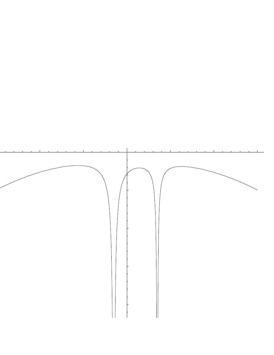
32.19 We plot here the potential along the line connecting the primaries,
in units where
M + m = 1, R = 1
and for the case
ν = 0.3
.
PHY411 S. G. Rajeev
39
-3
-2
-1
1
2
3
-20
-15
-10
-5

40
PHY411 S. G. Rajeev
32.20 The same method as before shows that these three solutions are
unstable: they correspond to saddle points of the potential. As a function of
x
they are maxima and as a function of
y
,
L
1
, L
2
, L
3
are minima.
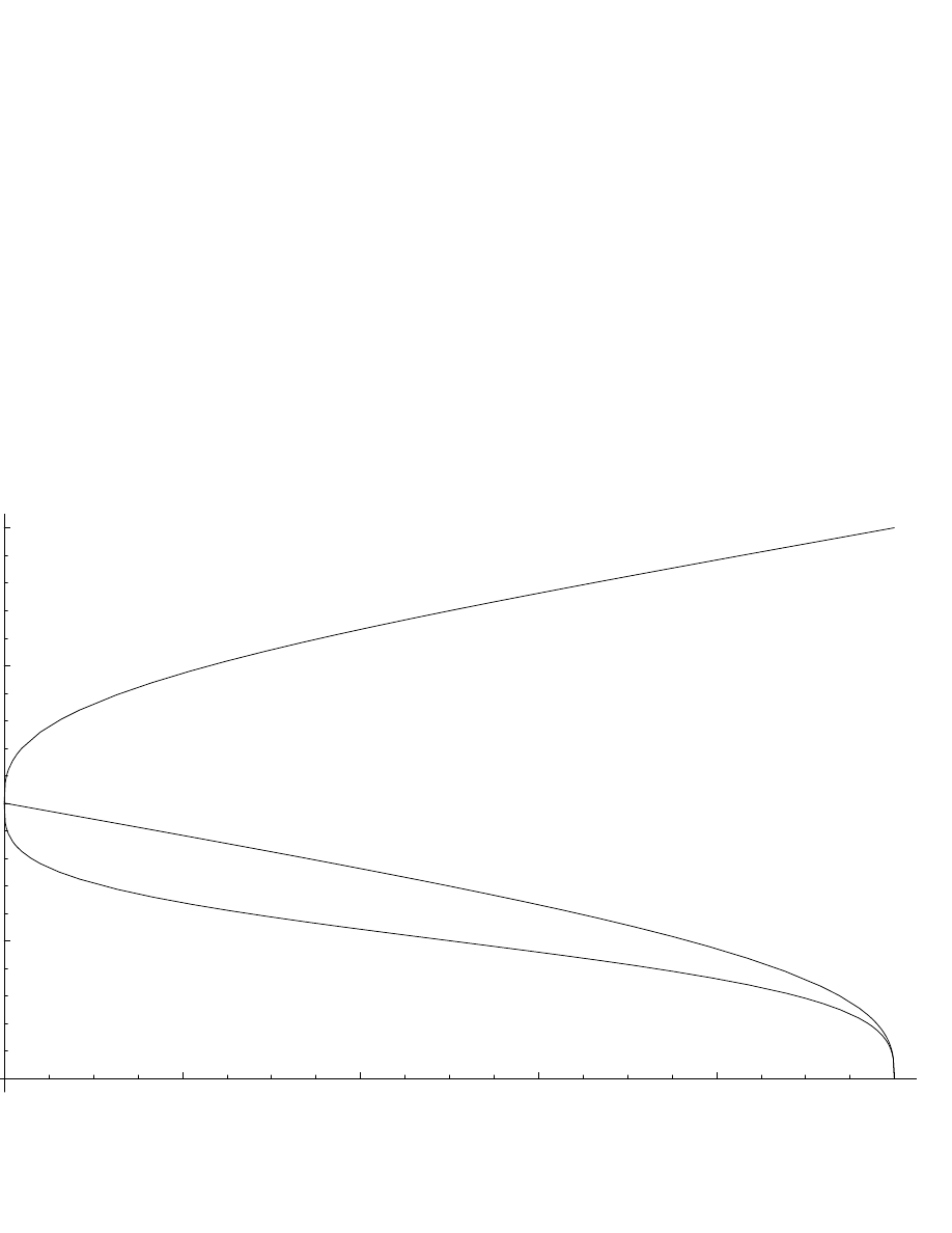
32.21 Here is a plot of the
r
1
-co-ordinate ( in units of
R
) of the Lagrange
points
L
1
, L
2
, L
3
as a function of
ν
:
PHY411 S. G. Rajeev
41
0.2
0.4
0.6
0.8
1
0.5
1
1.5
2

42
PHY411 S. G. Rajeev
32.22 For the Earth-Moon system
µ
∼
1
81
and
R
∼ 3 × 10
5
km; hence
the points
L
1,2
are at a distance of
5
× 10
4
km from the Moon.

Chapter 10
Time Dependent Linear
Systems
•Often we are interested in small corrections to a given orbit: a generaliza-
tion of the perturbations around static solutions that we discussed in the last
chapter. In particular we are interested in the staibility of periodic orbits.
•These problems arise for example in celestial mechanics. The orbit of the
moon around the earth is periodic with a period of about 28 days. The
correction due to the gravitational field of the Sun can be thought of as
a small perturbation, which will lead to a linear differential equation with
periodic coefficients (Hill’s equation).
•The equations of motion of the Lagrangian
L(q, ˙
q) =
1
2
˙
q
i
˙
q
i
− V (q)
can be
written as a first order system
d
dt
q
i
= p
i
,
d
dt
p
i
=
−
∂V
∂q
i
.
Here,
p
i
is the momentum conjugate to
q
i
. Let
(q
0i
(t), p
0i
(t))
be a solution
and
q
i
(t) = q
0i
(t) + ξ
i
(t), p
i
(t) = p
0i
+ η
i
(t)
be another solution close to it. If
(ξ(t), η(t))
is infinitesimally small, we can linearize the equations of motion:
d
dt
ξ
i
= η
j
,
d
dt
η
i
=
−
∂
2
V
∂q
i
∂q
j
(t)ξ
j
.
•If
z = (ξ, η)
we can write this as a linear system of differential equations
43

44
PHY411 S. G. Rajeev
with time dependent coefficients:
d
dt
z = A(t)z,
A =
0
1
−V
00
0
.
•If
A
is a constant matrix the solution is
z(t) = e
At
z(0) =
"
∞
X
n=0
(At)
n
n!
#
z(0).
The series converges because it can be dominated term by term by the ex-
ponential series
∞
X
n=0
(
|A|t)
n
n!
where
|A| = sup
u
||Au||
||u||
is the norm of the matrix. (
|A|
is basically the
largest magnitude of the eigenvalues of
A
.)
•There is a similar convergent power series expansion for the solution of the
time dependent linear system. This is in fact a way to prove the existence of
solutions of such a syste,. It also proves the real analyticity of the solution
as a function of time, provided
A(t)
itself is real analytic.
•The trick is to write the ODE as a system of integral equations:
z(t) = z(0) +
Z
t
0
A(t
1
)z(t
1
)dt
1
and iterate it to get an infinite series:
z(t) = z(0) +
Z
t
0
A(t
1
)z(0)dt
1
+
Z
t
0
dt
2
Z
t
2
0
dt
1
A(t
2
)A(t
1
)z(0) +
· · ·
Z
t
0
dt
n
−1
Z
t
n
−1
0
dt
n
−2
· · ·
Z
t
2
0
dt
1
A(t
n
−1
)
· · · A(t
2
)A(t
1
)z(0)
+
Z
t
0
dt
n
Z
t
n
0
dt
n
−1
· · ·
Z
t
2
0
dt
1
A(t
n
)
· · · A(t
2
)A(t
1
)z(0) +
· · · .
Now, suppose
|A(t
1
)
| < K(t)
for all
0 < t
1
< t
. Then the
n
th term is
smaller than
[K(t)t]
n
n!
.

PHY411 S. G. Rajeev
45
This proves the convergence of the infinite series, again by dominating it
term by term by the exponential series.
•The
path ordered exponential
of
A
is defined by the infinite series
ˆ
e
R
t
0
A(t
1
)dt
1
=
∞
X
n=0
Z
t>t
n
>t
n
−1
···t
1
>0
dt
n
· · · dt
1
A(t
n
)A(t
n
−1
)
· · · A(t
2
)A(t
1
).
If
A(t)
is constant, this becomes just the usual exponential series for
e
At
. The times in the integration are ordered; if
A(t)
is a constant we can
replace this by the integral over
[0, t]
except we divide by the number of
permutations
n!
. This is how you get the exponential series.
•If
A(t)
is of zero trace for all time, its path ordered exponential is of
determinant one. For constant matrices it follows from the identity
det e
A
= e
trA
.
More generally, for any matrix valued function
g(t)
d
dt
log det g(t) = tr
"
d
dt
g(t)
#
g
−1
(t).
(Prove this by first order perturbation theory!). If
g(t) = ˆ
e
R
t
0
A(t
1
)dt
1
, we
have
"
d
dt
g(t)
#
g
−1
(t) = A(t),
g(0) = 1.
From this it follows that
det g(t) = 1
if
trA(t) = 0
.
•Now suppose that
A(t)
is periodic:
A(t + T ) = A(t)
. It doesnt follow
that its path ordered exponential
g(t)
is periodic. But it will be periodic
upto a factor:
g(t + T ) = M g(t)
where
M = g(T ).
The point is that
g
1
(t) = g(t + T )
and
g(t)
satisfy the same differential
equations; the only difference is in the initial conditions:
g
1
(0) = g(T )
whereas
g(t0) = 1
. So the solutions are the same upto a constant multiple.

46
PHY411 S. G. Rajeev
•A solution
q
0
(t)
is stable if the equation for perturbations around it has
always bounded solutions. Now, after each period the solution changes by a
factor of
M
:
z(t + nT ) = M
n
z(t).
The question is whether the sequence
M
n
is bounded. This is true whenever
the eigenvalues of
M
are distinct and are all of magnitude less than or equal
to one.

Chapter 11
Hamiltonian Mechanics
•We start with the notion of a Legendre transform in calculus. Let
f :
R
n
→ R
be a
convex
function; i.e., the second derivative
f
00
is a positive
matrix everywhere. Then its Legendre transform
ˆ
f (p)
is defined by
ˆ
f (p) = extr
x
[p
· x − f(x)] .
Here,
extr
x
denotes the extremum in the variable
x
. There is a unique
extremum for the quantity in the brackets because
f
00
(x)
is invertible ev-
erywhere. The extremum is the solution of the non-linear equations:
f
0
(x) = p
which has a solution (
the inverse function theorem of calculus
) in a domain
where
f
00
(x)
is non-zero.
•The Legendre transform is itself a convex function. The transform is its
own inverse:
ˆˆ
f (x) = f (x).
•A useful example is a quadratic function,
f (x) =
1
2
x
T
Ax
for some positive matrix
x
. Then the extremum is at
x
0
= A
−1
p
and
ˆ
f (p) =
1
2
p
T
A
−1
p.
47

48
PHY411 S. G. Rajeev
The above properties are obvious here.
•More generally the extrema of
f
and
ˆ
f
are given by the pair of equations
p = f
0
(x),
x = ˆ
f
0
(p).
The solutions of these equations are inverse functions of each other. (
Prove
this!
).
Thus the extremization problem has two equivalent formulations,
either in terms of
f
or
ˆ
f
.
•The Legendre transform is an approximation to the Fourier transform; it
is the leading order of the stationary phase approximation. But we wont
puruse this matter here.
•The Legendre transform arises in many physical situations where we an
extremization problem has an equivalent formulation in two ‘dual’ descrip-
tions. (If we had regarded
f
as a concex function ona vector space
V
, the
Legendre transform would have been a convex function on the dual space.)
•For example, in thermodynamics, pressure and volume are dual variables.
The internal energy can be viewed either as a convex function of pressure or
of volume; the two versions of the energy are Legendre transforms of each
other.
•In mechanics, we are interested in an extremum of a function of an infinite
number of variables: the action viewed as a function of the position and ve-
locities. There is a ‘dual’ formulation of this problem where the velocities are
traded for conjgate variables called momenta. This gives a new formulation
of the action principle, the
Hamitonian formulation
.
•Recall that the action is
S[q] =
Z
L(q(t), ˙
q(t), t)dt.
By analogy to the above, let us define the Legendre transform of the la-
grangian with respect to the velocities:
H(q(t), p(t), t) =
X
i
p
i
(t) ˙
q
i
(t)
− L(q(t), ˙q(t), t)
where the
p(t)
and
˙
q(t)
are related by the condition that the r.h.s be an
extremum:
p
i
=
∂L
∂ ˙
q
i
(t)
.

PHY411 S. G. Rajeev
49
(We are supposed to solve thse equation to eliminate
˙
q
in terms of
p
in
the formula for
H
.) This function
H(q, p, t)
is the
hamiltonian
.
•Conversely the lagrangian is the Legendre transform of the hamiltonian.
The action is then
S[q, p] =
Z
"
X
i
p
i
˙
q
i
(t)
− H(q(t), p(t), t)
#
dt
The equations of motion in this alternative picture are obtained by varying
q
and
p
as independent variables:
dq
i
dt
=
∂H
∂p
i
,
dp
i
dt
=
−
∂H
∂q
i
.
These are
Hamilton’s equations
.
•
Example
Let
L =
1
2
m ˙
q
2
− V (q)
, the Lagrangian of a partcle of mass
m
in a potential
V (x)
. The variable
p
is just the momentum
p = m ˙
q
and
H
the energy:
H(q, p, t) =
p
2
2m
+ V (q).
Whenever the Lagrangian does not depend explicitly on time, the hamilto-
nian is the energy.
•Hamilton’s equations are a system of
2n
first order differential equations
for a system with
n
degrees of freedom.The set of initial conditions is a
manifold of dimension
2n
, called the phase space. Through each point in
this space is a unique curve which is the solution of the equations of motion.
•
Example
The system with hamiltonian
H =
p
2
2m
+
1
2
kx
2
is the simple
harmonic oscillator. The equations of motion are linear
dq
dt
=
p
m
,
dp
dt
=
−kq.
The solutions are ellipses in the plane
(q, p)
.
•Any observable quantity of a mechanical system can be expressed as a
function of co-ordinates and momenta; i.e., as functions on the phase space.
( We exclude for now any explicit dependence on time for
f
as well as the
hamiltonian.) It is interesting to ask how such an observable changes with
time:
df
dt
=
X
i
∂f
∂q
i
dq
i
dt
+
X
i
∂f
∂p
i
dp
i
dt
.

50
PHY411 S. G. Rajeev
By Hamilton’s equations,
df
dt
=
X
i
∂f
∂q
i
∂H
∂p
i
−
∂f
∂p
i
∂H
∂q
i
!
.
•The quantity in the brackets is of fundamental significance in classical
mechanics. It is called the
Poisson bracket
. In general the Poisson bracket
of a pair of observables is defined by
{f, g} =
X
i
∂f
∂q
i
∂g
∂p
i
−
∂f
∂p
i
∂g
∂q
i
!
.
•Thus Hamilton’s equations are equivalent to the statement
df
dt
=
{f, H}
for any observable. In particular a
conserved quantity
is a function tat has
no explicit time dependence and also has zero total time derivative: in other
words a conserved quantity has zero Poisson brackets with the hamiltonian:
{f, H} = 0
•The Poisson bracket satisfies the identities
{f, g} = −{g, f},
{{f, g}, h} + {{g, h}, f} + {{h, f}, g} = 0,
{f, gh} = {f, g}h + g{f, h}.
The first identity is obvious. The second (
the Jacobi identity
) is hard, but
straightforward to prove by a long calculation. The last is just the statement
that the Poisson brackets is linear in the first derivatives of the functions.
•It is more important to know why these are interesting identities; indeed
why this whole way of thinking of mechanics is useful. The understanding
of any mechanical system starts with that of its conserved quantities. Some
of them will be obvious but others can be quite obscure at first. The above
identities show for example that the product (
easy!
) and the Poisson brackets
(
use the Jacobi identity!
) of two conserved quantities are also conserved.
•But that is just the beginning. Imagine that we could find a complete set
of observables which are either constant in time, or depend linearly on time.

PHY411 S. G. Rajeev
51
•Then using these observables as co-ordinates the solution of the system
would be as trivial as that for the free particle. Thus instead of trying to solve
differential equations directly we shift to looking for appropriate changes of
co-ordinates.
•But what are the allowed changes of co-ordinates that preserve Hamilton’s
equations;i.e., so that the new co-ordinates
(Q, P )
also satisfy
dQ
i
dt
=
∂H
∂P
i
,
dP
i
dt
=
−
∂H
∂Q
i
.
A straightforward calculation will show that the conditions are
{Q
i
, Q
j
} = 0 = {P
i
, P
j
},
{Q
i
, P
j
} = δ
i
j
.
(Here
δ
i
j
is the
Kronecker
symbol, which is
1
for
i = j
and
0
otherwise.)
Variables that satisfy these relations are said to be
canonical
: they are the
“correct” co-ordinates to use in classical mechanics.
•There is an enormous freedom within the world of canonical co-ordinates:
we can even mix momenta and position with each other. If we can find
canonical co-ordinates
(θ
i
, I
i
)
such that the hamiltonian only depends on
the ‘momenta’
I
i
we have solved the equations of motion. For in these
co-ordinates,
dI
i
dt
= 0,
dθ
i
dt
=
∂H
∂I
i
.
•Discovering such
normal co-ordinates
is the holy grail of classical mechan-
ics: once we find such a co-ordinate system the equations are solved in a
trivial way. The whole question is then whether such co-ordinates exist and
if so how to find them.
•The key to understanding these issues is, surprisingly, geometry. Let us
first look at the hamrmoic oscillator:
H =
p
2
2m
+
1
2
kq
2
.
We saw that the orbits are ellipses in the phase plane: these are just the
curves of constant energy:
p
2
2m
+
1
2
kq
2
= E.

52
PHY411 S. G. Rajeev
The particle moves along this ellipse as time evolves. In this case we know
explicit answer:
q(t) =
2E
k
1
2
cos[ω(t
− t
0
)],
p(t) =
√
[2mE] sin[ω(t
− t
0
)]
Thus the change of variables
q = A cos θ, p = B sin θ
suggests itself, where
A, B
are the axes of the ellipse. What is the conjugate
I
of the angle
variable
θ
? It turns out to be (upto a constant) the
area of the ellipse!
.
To see this, let us think of
A, B
as functions of
I
. Then the canonical
relations among the pairs
(q, p)
and
(θ, I)
give
{q, p} =
∂q
∂I
∂p
∂θ
−
∂q
∂θ
∂p
∂I
= 1.
which gives
A(I)B
0
(I) + A
0
(I)B(I) = 1, A(I)B
0
(I)
− A
0
(I)B(I) = 0.
In other words
AB = I
or
I = 2Eω
. The area of the ellipse is the product
of the semi-axes times
π
. Thus the variable
I
is just the area of the ellipse
upto a factor of
π
.
•Why do we get such a geometrical answer? The point is that
{θ, I} =
∂(θ, I)
∂(q, p)
is just the Jacobian of the transformation
(q, p)
7→ (θ, I)
. Thus canonical
transformations preserve the area. Indeed, the area of a curve can be written
either as
R
γ
pdq
or
R
γ
Idθ
as long as ther two co-ordinates are canonically
related.
•Thus we can generalize the above ideas to an arbitrary conservative system
with one degree of freedom. The curves
H(p, q) = E
enclose an area
I(E) =
R
γ
E
pdq
. This area can be chosen as one of the co-ordinates in phase
space. It is obviously a conserved quantity since it depends only on energy.
Conversely energy can be thought of as a function of
I
:
H = f (I)
. The
conjugate variable
θ
will depend on time linearly since it satisfies Hamilton’s
equations:
dθ
dt
=
∂f (I)
∂I
.
Indeed
θ = ω(I)[t
− t
0
]
where the frequency is
∂f (I)
∂I
. In the case of the
harmonic oscillator this frequency is even independent of energy or
I
; but
in general this is not true.

Chapter 12
Hamilton-Jacobi Theory
•Suppose we are presented a system with hamiltonian
H(q, p)
in some
canonical co-ordinate system
(q
i
, p
i
)
. If we can find a new canonical co-
ordinate system
(θ
i
, I
i
)
such that the hamiltonian depends only on the
momentum variables
I
i
, then we have solved the equations of motion. For,
in this system, the Hamiltons equations are
dI
i
dt
= 0,
dθ
i
dt
= ω
i
(I)
where the frequencies are
ω
i
(I) =
∂H(I)
∂I
i
. Such a system will be called
normal co-ordinate system
; they are also called
action-angle
variables.
•The motion is on surfaces of constant
I
i
, on which the
n
variables
θ
i
are
co-ordinates; they depend linearly on time. Often this is a surface of finite
volume and the co-ordinates
θ
i
are some sort of angles: the surface is a
torus. Indeed, there is a vector field (the velocity) which is everywhere non-
zero and has constant components in these co-ordinates. The only compact
surface on which that is possible is a torus. It is conventional to choose the
period of each angle to be
2π
. These surfaces of constant
I
i
are called
invariant torii
(they are invariant under time evolution.)
•If there is a real number
ω
and non-zero integers
n
i
such that
ω
i
= n
i
ω
,
the motion is periodic. But generically, the frequencies are not related: there
is no set of integers such that
P
i
ω
i
= 0
. In this case there is a period
2π
ω
i
in each variable separately, but no common period for the motion as a whole:
it is
quasi-periodic
.
•A hamiltonian for which such a normal co-ordinate system exists is said
to be
integrable
. It is found that such hamiltonians are ‘rare’: under small
53

54
PHY411 S. G. Rajeev
perturbations we will lose this property. Still much of what we know about
mechanics comes from such examples.
•A co-ordinate independent characetrization of integrablity is that the whole
phase space can be split up (‘foliated’) into invariant torii.
•Thus much of mechanics is about the search for the normal co-ordinates
or equivalently the invariant torii. Even when they dont exist the attempt
to construct them (by perturbing around an integrable limiting case ) will
reveal deeper structure of the system and even about mechanisc in general.
•Under small perturbations of an integrable system, some of the torii remain
invariant although they suffer some deformation: the phase space is divided
up into regions bounded by these surviving torii. (Of course by time evolution
one can never cross an invariant torus.) To any compact subset of the phase
space, we can associate the ratio of the volume of the points that lie on
invariant torii to the total volume. This ratio can be made to approach
one by choosing the strength of the perturbation small enough. Thus small
perturbations dont destroy totally the integrability of a system: ‘most’ initial
data still lie on invariant torii. This is believed to ‘explain’ the stablity of
the solar system in spite of the fact that it is not an integrable system: it
is a small perturbation of an integrable system so most orbits are still either
on invariant torii or are bounded by them.
•What I gave above is a paraphrasing of one of the most profound results
in all of mechanics, may be even physics: the Kolmogorov-Arnold-Moser
theorem. We will say more about it later.
•However the structure of the invariant torii is enormously compicated even
with a small perturbation: inside each invariant torus there can be another
and so on ad infinitum: there is a self-similar structure for the typical system.
Even this case of small perturbations around an integrable system is poorly
understood still.
•There are mechanical systems which as far from being integrable of course.
An extreme example would be an
ergodic system
for which each orbit is
dense on the energy surface. Clearly then there are no constants of the
motion other than energy and no invariant torii either. These systems are
believed to be described by statitical mechanics.
•There is a wide variety of possiblities in between. Of special interest are
periodic orbits. For generic systems there are only a countable number of
these (periodic orbits are ‘rare’). The actions of these periodic orbits form a
kind of
classical spectrum
for a mechanical system.

PHY411 S. G. Rajeev
55
•Indeed Gutzwiller has shown that this classical spectrum of periodic orbits
determines the eigenvalues of the quamtum mechanical hamiltonian, in the
limit as
¯
h
→ 0
.
•So how does one look for normal co-ordinates? Suppose we are given the
hamiltonian as a function of some canonical co-ordinates
(q, p)
. We seek
new canonical co-ordinates
(θ, I)
such that the hamiltonian is independent
of the
θ
(‘angle’) variables. The canonical transformation from
(q, p)
to
(θ, I)
must have a generating function
W (q, I)
, such that
p
i
=
∂W (q, I)
∂q
i
,
θ
i
=
∂W
∂I
i
.
•Putting this into the hamiltonian, we get a first order partial differential
equation for
W
:
H(
∂W
q
i
, q) = E.
This is called the
Hamiltonian-Jacobi equation
. If we can solve this equation
we have found the canonical transformation to the normal co-ordinates, which
is the same as solving the equations of motion.
•The constants of integration in solving this equation are the ‘action’ vari-
ables
I
i
.
•Thus we have transformed the original system of oridnary differential equa-
tions (Hamilton’s equations) to a single first order non-linear partial differen-
tial equation. In fact this is a reversible process: any single first order partial
differential equation can be turned to a system of ordinary differential equa-
tions. The curves that solve this system are the ‘characteristics’.
•Let us look at an examples from outside of mechanics, the propagation of
waves in an inhomogenous medium. We will think of them as light waves but
the story is the same for sound waves or water waves. The wave equation is
then
−∇
2
φ +
n
2
(x)
c
2
∂
2
∂t
2
φ = 0.
( We have ignored the polarization of light; also some additional approxima-
tions about the gradient of
n
have been made. See Born and Wolf for the
complete story.) Here
n
is the refractive index and
c
is the velocity of
light.

56
PHY411 S. G. Rajeev
•For monochromatic waves,
∇
2
ψ + k
2
n
2
(x)ψ = 0
where
k
is the wave number. Put
ψ = e
ikW
to get
−(∇W )
2
+ n
2
+
1
k
2
i
∇
2
W = 0.
If the variational of the refractive index over one wavelength is small, we
can ignore the second derivative term of
W
a first order partial differential
equation. The function
W
(called the
eikonal
) satisfies
(
∇W )
2
= n
2
.
The analogy to the Hamilton-Jacobi equation is clear.
•It is as if we have a hamiltonian
H(x, p) =
1
2
[p
2
− n
2
]
. The equations for
the characteristics are
dx
dτ
= p,
dp
dτ
=
∇n
2
.
These are the equations for the light rays. This formulation is called
Hamil-
tonian optics
. There is a conjugate description in terms of Langrangians
as well. Determining rays is helped by the existence of
integral invariants
which are the analogues of conserved quantities.
•The eikonal equation is the approximation to the wave equation in the limit
of short wavelength. Is it possible to think of the Hamilton-Jacobi equation
as an approximation to a wave equation? Let
H(p, q) =
p
2
2m
+ V (q)
. We
would have by analogy
ψ = e
i
¯
h
W
.The constant
¯
h
has the dimensions of
action since that is the dimension of
W
in the H-J equation.
−
¯
h
2
2m
∇
2
ψ + V (q)ψ = Eψ.
This is just the Schrodinger equation;
¯
h
is Planck’s constant!. Hamilton
had some inkling of the existence of such a wave mechanics. But at that time
there was no experimental reason to doubt the absolute validity of Newtonian
mechanics.
•
Example
Let us solve the Kepler problem this way. In spherical polar
co-ordinates
H =
1
2m
"
p
2
r
+
p
2
θ
r
2
+
p
2
φ
r
2
sin
2
θ
#
+ V (r, θ, φ).

PHY411 S. G. Rajeev
57
As long as the potential is of the form
V = a(r) +
b(θ)
r
2
+
c(φ)
r
2
sin
2
θ
a solution of the form
W = R(r) + Θ(θ) + Φ(φ)
exists. This is the method of
separation of variables
. The ordinary differ-
ential equations for the functions
R, Θ, Φ
can be solved in terms of elliptic
functions. For details see Landau and Lifshitz.
•If we can solve the H-J equations, and determine the normal co-ordinates,
we can solve the equations of motion completely. Such systems are said to
be
integrable
. It turns out that not all systems are integrable.
•An integrable system with
n
degrees of freedom will have
n
conserved
quantities: the ‘action’ variables. In fact it will have
n
conserved quantities
in
involution
: their mutual Poisson brackets are zero. Conversely whenever
there and
n
independent conserved quantities in involution, a system with
n
degrees of freedom is integrable.
•The surfaces defined by
I
i
=
constant are torii: they admit vector fields
that are non-zero everywhere,
∂
∂θ
i
.The existence of these
invariant torii
is
an abstract characterization of integrability.
•In the normal co-ordinates, the solutions of the equations of motion are
real analytic in time. Indeed, this appears to be another characetrization of
integrability: if the solutions of the equations of motion are real analytic in
time, the system is integrable. But I dont know of a rigorous theorem along
these lines.

Chapter 13
Birkhoff Normal Form
•See F. G. Gustavson Astonomical Journal Vol 71, 670 (1966) for a beautiful
exposition of these ideas.
•We now start the study of classical systems that are not integrable. Sup-
pose that a system has a stable equilibrium point; Near this point it is well
approximated by a harmonic oscillator; there are canonical co-ordinates such
that the hamiltonian is
H(q, p) =
1
2
X
i
ω
i
(p
2
i
+ q
2
i
) + O(3)
upto terms that are cubic in the co-ordinates.
•The higher order terms describes the non-linearities in the equations of
motion. We can regard the hamiltonian as a power series
H(q, p) =
∞
X
r=2
H
r
(q, p)
where
H
r
(q, p) =
P
|A|+|B|=r
H
AB
q
A
p
B
is a homogenous polynomial of order
r
in
(q, p)
. Here
A =
{A
1
, A
2
· · · A
n
}
is a multi-index and
q
A
= q
a
1
1
· · · q
a
n
n
etc. Also,
|A| = a
1
+ a
2
· · · + a
n
, so that the degree of the polynomial is
r =
|A| + |B|
. Of course
H
2
(q, p) =
1
2
P
i
ω
i
(p
2
i
+ q
2
i
)
.
•Even if the hamiltonian is a smooth function, this series may not converge;
it may not be a real analytic function. Still this series makes sense as a
‘formal power series’. ( See the appendix for a discussion of formal power
series.)
•We say that the hamiltonian is
in normal form upto order
s
if
DH
r
= 0
for r
≤ s,
58

PHY411 S. G. Rajeev
59
where
D =
X
i
ω
i
q
i
∂
∂p
i
− p
i
∂
∂q
i
!
.
In other words
H
AB
= 0
for
|A| + |B| ≤ s
unless
X
i
ω
i
[a
i
− b
i
] = 0.
•To understand what this means, note that the operator
D
is
D =
X
i
ω
i
∂
∂θ
i
where
θ
i
are the angular co-ordinates conjugate to
I
i
= q
2
i
+ p
2
i
. The
simplest case is when the frequencies
ω
i
are
linearly independent
to order
s
: there are no integers
k
i
, with
|k
1
| + |k
2
| · · · |k
n
| ≤ s
such that
X
k
i
ω
i
= 0.
Then for a hamiltonian of normal form, the hamiltonian is independent of
θ
i
and
I
i
are conserved to order
s
: they serve as approximate action-angle
variables.
•In the case where the frequencies are linearly dependent there may be reso-
nances, and the hamiltonian may depend on additional variables and we wont
have enough conserved quantities to ‘solve’ the system even approximately.
•
Theorem
Given any hamiltonian
H =
1
2
P
i
ω
i
[q
2
i
+ p
2
i
] + O(3)
and any pos-
itive integer
s
, there exists a canonical transformation to new co-ordinates
(Q
i
, P
i
)
such that the new hamiltonian
Γ(Q, P )
is of normal form to order
s
.
•Thus we can solve any classical mechanical system to arbitrary order if the
frequencies are linearly independent.
•The proof proceeds by induction; in fact we will give an algorithm to
construct the necessary canonical transformation order by order. Suppose
the hamiltonian is already in normal form to some order
s
− 1
. ( Right at
the start we have
s = 3
.) Consider a canonical transformation generated
by
P
i
q
i
P
i
+ w
s
(q, P )
where
w
s
(q, P )
is a homogenous polynomial of order
s
in the new momenta and old co-ordinates. The old co-ordinates
q
can
be eliminated in terms of the new ones
Q
using
Q
i
= q
i
+
∂w
s
∂P
.

60
PHY411 S. G. Rajeev
The new hamiltonian is determined by
H(q, P +
∂w
s
∂q
) = Γ(q +
∂w
s
∂P
, P ).
If we equate terms of order
s
of this equation we get
Dw
s
(q, P ) = Γ
s
(q, P )
− H
s
(q, P ).
Now we show that
w
s
can be chosen such that
Γ
s
is of normal form; i.e.,
in the kernel of
D
.
D
is a linear operator in the space of homogenous
polynomials
V
s
. It is not invertible, but is antisymmetric so that we have
a decomposition
V
s
= ker D + range D
. In particular we can split
H
s
=
K
s
+ R
s
where
K
s
∈ ker D
and
R
s
∈ range D
. Thus if we determine
w
s
by solving
Dw
s
= R
s
, we have
Γ
s
= R
s
; i.e.,
Γ
s
is in normal form. This
completes the proof.
•The solution of the equation
Dw
s
= R
s
is facilitated by diagonalizing
D
. Being anti-symmetric, it is diagonalized by complex linear combinations
z
j
= q
j
+ ip
j
, ¯
z
j
= q
j
− ip
j
:
Dz
A
¯
z
B
= i
X
i
[a
i
− b
i
]ω
i
z
A
¯
z
B
.
Thus the pseudo-inverse of
D
may be defined to be
D
−1
z
A
¯
z
B
=
(
0
if
P
i
[a
i
− b
i
]ω
i
= 0
1
i
P
i
[a
i
−b
i
]ω
i
z
A
¯
z
B
otherwise
)
.
Then we just have to express
H
s
as a polynomial in
z, ¯
z
and then set
w
s
=
−D
−1
H
s
.
•This will give us the hamiltonian as a function of
(q, P )
. We must now
eliminate
q
, solving
q
i
= Q
i
−
∂w
s
(q, P )
∂P
i
as a power series in
(Q, P )
. Substituiting into the hamiltonian will give us
an infinite series for
Γ
. Gustavson has worked out the following formula for
the term of order
r
in
Γ
Γ
r
= H
r
+
X
l
− |j| + |j|(s − 1) = r
1
≤ |j| ≤ l ≤ r
l
≥ 2, s ≥ 3
1
j!
∂
|j|
H
l
∂P
j
∂w
s
∂q
!
j
−
∂
|j|
Γ
l
∂q
j
∂w
s
∂P
!
j

PHY411 S. G. Rajeev
61
Here
j! = j
1
!j
2
!
· · · j
n
!
etc.
To order less than
s
this says that
Γ
r
= H
r
. To
order
s
this is the equation that determines
w
s
. In higher orders this gives
the terms of the new hamiltonian in terms of the old one recursively. This
formula can be translated into a symbolic computer program.
•By iterating this procedure, the hamiltonian can be reduced to normal
form to any order.
•If the frequencies are linearly independent to all orders, we can construct a
complete set of conserved quantities
I
i
= Q
2
i
+ P
2
i
as a formal power series
in the original co-ordinates
(q, p)
. If this power series were convergent, we
would have been able to show that every non-resonant classical mechanical
system is integrable. But it turns out that typically, the series are diver-
gent. Still, if the perturbations are small enough this procedure gives a good
approximate solution.

62
PHY411 S. G. Rajeev
Appendix: Formal Power Series
•A convergent power series
f (z) =
∞
X
n=0
f
n
z
n
determines an analytic function. The sum, product and derivative of analytic
functions translate into operations on the coefficients:
[f + g]
n
= f
n
+ g
n
,
[f g]
n
=
X
k+l=n
f
k
g
l
,
[f
0
]
n
= (n + 1)f
n+1
•These operations involve only a finite number of coefficients. Hence the
space of infinite sequences
(f
0
, f
1
,
· · ·)
is a commutative ring with derivation.
If the sequence is rapidly decreasing, this corresponds to an analytic function;
otherwise the sequence can be thought of as generalizing the notion of a
function, a
formal power series
. In many mathematical situations, this ring
of formal power series a good substitute for the ring of functions of one
variable. We may still write occasionally
f (z) =
X
n
f
n
z
n
but of course the quatity
f (z)
is not always a function: there may be no
meaning to evaluating it at some value of
z
.
•The idea generalizes to an arbitrary number of variables: the coeffiecients
become symmetric tensors:
f (z) =
X
f
i
1
···i
r
z
i
1
· · · z
i
r
.
An equivalent description is in terms of multi-exponents
A = (a
1
,
· · · a
n
)
:
f (z) =
∞
X
A=0
f
A
z
a
1
1
· · · z
a
n
n
.
•A divergent series might describe a function that is not analytic. A series
P
∞
n=0
f
n
z
n
is an
asymptotic expansion
of a function,
f (z)
∼
P
∞
n=0
f
n
z
n
if
there is a wedge
θ
1
< arg(z) < θ
2
such that
lim
|z|→0
z
−n
[f (z)
−
n
X
0
f
k
z
k
] = 0
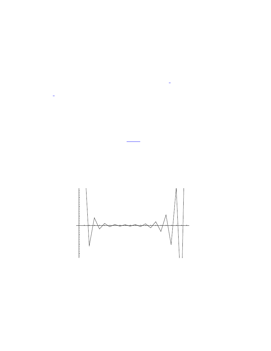
PHY411 S. G. Rajeev
63
for every
n
. The limit is taken along some ray within the wedge. The idea
is that the difference between
f (z)
and the sum of the first
n
terms is of
the same order as the
(n + 1)
th term, as long as
arg(z)
is within the range.
•An asymptotic series, unlike a convergent series does not determine the
function uniquely. For example we can always add
e
−
1
z
to any function
without changing its asymptotic series!. The point is that all the derivatives
of
e
−
1
z
are zero at the origin and yet it is not analytic.
•If additional information is available about the function we can determine
it from its asymtotic series. The ideas to do that involve integral transforms
(Borel transform) or Pade approximants.
•
Example
The series
f (z) =
P
∞
0
n!z
n
is not convergent. Yet it can be
thought of the Taylor series expansion of the function
f (z) =
Z
∞
0
e
−t
dt
1
− zt
.
In fact for moderate values of
|z|
(say
|z| < 0.1
) we can even find a good
approximation to the value of the function by the power series. (Exercise:
Write a small program to verify this. It is easy to do in Mathematica.) The
point is that the series starts to converge to the value of the function for a
finite number of terms before diverging away. The smaller the value of
|z|
,
the longer it is converging, and the better the approximation.
5
10
15
20
-0.006
-0.004
-0.002
0.002
0.004
0.006
The difference
f (z)
−
P
N
n=0
n!z
n
for
z =
−0.1
and various values of
N
. Note
that the error decreases at first then diverges for larger powers.
•Another example of this phenomenon is the Stirling expansion of the
Gamma function. The Gamma function has an essential singularity at infin-
ity, so cannot have a convergent power series expansion valid for large
z
.

64
PHY411 S. G. Rajeev
Yet, the Stirling formula gives very accurate numerical values for
|z|
greater
than about
10
. ( The Stirling expansion is not quite a power series; but after
some leading factors are removed it can be made into one.) Actually there
is an irony here. The inverse of the Gamma function is an entire function,
hence has a convergent power series expansion for
any
z
. So it would seem
reasonable that we calculate the value of
1
Γ(z)
by the power series and just
find the reciprocal to find the value of
Γ(z)
. However, the Stirling series,
which is divergent, gives more accurate answers than the convergent series
once
|z|
is moderately large
|z| > 10
.
•So we should not dismiss divergent series as useless. What is going on here
is that the usual notion of convergence is too restrictive: it requires the series
to give a good approximation for all values of
z
within a circle. But often
we are only interested in a good approximation within a pie-shaped region,
for example containing the real axis. Then the appropriate approach is to
seek an
asymptotic series
.
•Thus the weakest notion is that of a formal power series: it may not
represent any function. Next weakest is that of the asymptotic series, which
will determine the function upto one all of whose derivatves at the origin are
zero. The strongest is a convergent power series which uniquely determines
the function of which it is the Taylor series expansion.

Chapter 14
The Henon-Hiles Potential
•There are a handful of integrabel systems that are usually used to learn
classical mechanics. Yet the vast majority of systems are not integrable. We
still need to work out specific examples to learn about the behavior of such
systems. Examples arise from application to various areas of physics. In this
chapter we will study an example arising from astronomy, the
Henon-Hiles
system
: (M. Henon and C. Heiles, Astronomical Journal 69, 73, (1964).)
H =
1
2
[ ˙x
2
+ ˙
y
2
] +
1
2
[x
2
+ y
2
] + x
2
y
−
1
3
y
3
•This is supposed to describe gravitational potential seen by a star in the
center of a globular cluster. Its importance to us is that it is not integrable
and is well studied; we will not delve into the underlying astronomy.
•The origin is a stable equilibrium point; the frequencies are equal, so that
the system is resonant. Still, because it has only two degrees of freedom, it is
formally integrable by the Birkhoff-Gustavson method. Gustavson compared
the true behavior ( as determined by numerical calculations) to that predicted
by the formal power series method. The results are quite instructive and are
believed to be representative of all non-integrable systems.
•The phase space is four dimensional. Since the system is conservative, the
dynamics takes place on a three dimensional submanifold of constant energy.
If
E
≤
1
6
these surfaces of constant energy are bounded. (In general the
potential is unbounded below). If we had one more conserved quantity (
integral of motion) we would be able to solve the system.
•The Birkhoff-Gustavson procedure provides another such integral as a for-
mal power series. Suppose the hamiltonian has been reduced to normal form
65

66
PHY411 S. G. Rajeev
Γ(Q, P )
. Suppose also that there are
r
linear relationsa among the fre-
qoencies
Aω = 0
. Then any function of the form
P
i
µ
i
[Q
2
i
+ P
2
i
]
is a
conserved quantity if
Aµ
i
= 0
. This is not the hamiltonian
Γ
: there
are many additional terms in the hamiltonian itself. Hence if there are
r
relations among the frequencies (the matrix
A
is of rank
r
) there will be
n
− r
independent solutions to the equation
Aµ = 0
, and an equal number
formal integrals independent of the hamiltonian.
•Thus any conservative system with two degrees of freedom is formally
integrable: there is always the hamiltonian, and even if there is resonance at
least one new integral.
•For the Henon-Hiles potential the new integral is just
1
2
[Q
2
1
+ P
2
1
+ Q
2
2
+ P
2
1
]
in terms of the new co-ordinates. We must then retrace our steps inverting
the canonical transformations to express this in terms of the old variables
(x, y, ˙x, ˙
y)
.
•It is hard to visualize dynamics in a four-dimensional space; even after
imposing conservation of energy we will have three dimensions. We can look
a cross-section of the phase space where one of the co-ordonates (say
x
) is set
equal to zero. The solution is a curve that will intersect the two dimensional
space at a countable number points.
•This can be viewed as a discrete dynamical system on its own right, de-
termined by a map
(y, ˙
y)
7→ φ(y, ˙y)
. Given an initial
(y, ˙
y)
we can find
an
˙x
for which
x = 0
. This initial condition determines a curve and the
next time it intersects the plane
x = 0
determines the new point
φ(y, ˙
y)
. This map is a canonical transformation.The iterations of this canonical
transformation describe a set of points on the plane
(y
n+1
, ˙
y
n+1
) = φ(y
n
, ˙
y
n
)
upon iteration.
•If there is a conserved quantity
I
(other than the hamiltonian) the points
(y
n
, ˙
y
n
)
will lie along the curves along which
I
is constant. This suggests
a numerical experiment to test the efficacy of the Birkhoff procedure. We
calculate the formal integral of motion to some order (eight in the work of
Gustavson.) Plot the cuvres along which this polynomial is a constant. Now
numerically calculate the orbit
(y
n
, ˙
y
n
)
of a point on such a curve. If the
orbit lie on the curve, the system behaves much like an integrable system:
we will have an
invariant curve
. If on the other hand the orbit wanders all
over some bounded region in the plane then it is ‘chaotic’. it does not lie on
an invariant curve and there can be no conserved quantity.
•The results of this numerical experiment performed by Gustavson are quite
striking. For small values of energy ( small departure from integrability) the

PHY411 S. G. Rajeev
67
orbits lie more or less on the level surfaces. But as the energy grows some
small islands (bounded regions) appear, within which the orbits are spread
out. However there are still many orbits that still lie on the level curves. As
energy grows to the the maximum value of
1
6
the entire allowed phase space
is filled by a single orbit.
•A finite fraction of the initial conditions remain on curves invariant un-
der time evolution for small perturbations. As the perturbations grows this
fraction decreases to zero. Eventually there are no invariant curves at all
left.
•This suggests that the Birkhoff series is not convergent or even asymptotic
to any conserved quantity. But all is not lost: certain curves may remain
under time evolution, although they can no longer be thought of as level
surfaces of any conserved quantity. This notion of an invariant curve is weaker
than that of a conserved quantity and is stable under small perturbations.
•The KAM theorem demonstrates in a systematicaly how to construct such
invariant surfaces.

Chapter 15
Area Preserving Maps
•Since the problem of understanding non-integrable systems is quite hard,
we should look first at the simplest non-trivial examples. Any conservative
hamiltonian system with one degree of freedom is integrable. So the simplest
such systems are of two degrees of freedom, like the Henon-Hiles system.
•If time is a discrete rather than a continuous variable, then even a system
with one degree of freedom may be chaotic.
Such systems arise in several natural ways:
(i) The Poincare section, (or restriction) two a dimensional subspace of a
hamiltonian system with more than one degree of freedom is a symplectic
(are preserving) map of the plane to itself.
(ii) A time dependent hamiltonian, periodic in time with period
T
,
H(q, p, t)
determines a symplectic map of the plane, the time evolution through one
period.
(iii) Consider a static magnetic field and a surface orthogonal to the field.
The integral curves of the magnetic field will return to the surface, and
provide a map of the surface to itself. This maps preserves magnetic flux. If
the magnetic field is viewed as a symplectic form on the surface, the map is
symplectic.
•Thus we are led to study a map
φ : R
2
→ R
2
which preserves area:
det ∂φ = 1
. An orbit of such a map is an infinite sequence of points satisfying
(q
n+1
, p
n+1
) = φ(q
n
, p
n
)
.
•
Example
The map
q
n+1
= q
n
+ p
n+1
,
p
n+1
= p
n
+ λ sin q
n
is called the
standard map
. It is easy to check that it is area preserving. We
68

PHY411 S. G. Rajeev
69
can regard (q, p)
as periodic with period
2π
; then this is a map of a torus
to itself.
•This can be thought of as the time evolution of a rotor that is ‘kicked’ at
periodic intervals; the hamiltonian is
H(q, p, t) =
1
2
p
2
+ k sin q
P
n
δ(t
− n)
.
In between two kicks the system evolves like a free particle. During a kick
the momentum is changed by
k sin q
.
•If
λ = 0
, this is an integrable system: just a rotor. The orbits lie on
circles with constant
p
. If
p
is rational
p =
N
D
(with
N, D
coprime)
the orbit is periodic with period
D
; then
N
is the number of rotations
around the
q
-axis in one such period. Even when
p
is not rational it can
be approximated by rational numbers: there will be a sequence of periodic
orbits that converge to any orbit.
•A
conserved quantity
for
φ
is a function
I(p, q)
with non-zero derivative
everywhere
dI
6= 0
and satisfying
I(q, p) = I(φ(q, p))
. If there is such
a conserved quantity, the discrete dynamical system is integrable. If
θ
is
the canonical conjugate of
I
, the map reduces to
(I, θ)
7→ (I, θ + α(I)
:
a rotation of
θ
by an amount that can depend on
I
. This is called the
normal form
of the map.
•For example, if we have a conservative hamiltonian system of one degree of
freedom, and
φ
is the time evolution through a finite interval, the hamilto-
nian itself would be such a conserved quantity.Then the co-ordinate system
(I, θ)
would be the action-angle variables.
•Suppose the discrete system is the restriction to integer values of time of
a continuous dynamical system: there are symplectic maps
φ
t
: R
2
→ R
2
such that
φ
t+s
= φ
t
(φ
− s)
. Then the infinitesimal time evolution arises
from a hamiltonian:
dq
t
dt
=
∂H
∂p
,
dp
t
dt
=
−
∂H
∂q
. This hamiltonian is then a
conserved quantity for
φ
and the system is integrable.
•In general it is not possible to reduce a system to normal form: there is no
conserved function. But there may be a conserved quantity in the sense of a
power series, which may not converge.
G. D. Birkhoff, Acta. Math. 43, 1
(1920)
is the definitive study of such maps. This work has been revived in
recent times by Kadanoff for example as a model of deterministic chaos.
•The main idea is that as a formal power series, it is possible to continue
orbit
(q
n
, p
n
)
to all real values of time
n
. Then by differentiation we will
get a ‘hamiltonian’ as a formal power series.
•As in the case of continuous systems, we start by expanding the map
φ
in
a power series around a fixed point. We can choose this to be at the origin.

70
PHY411 S. G. Rajeev
In the linear approximation we have
q
n+1
p
n+1
=
a
b
c
d
q
n
p
n
,
ad
− bc = 1.
In this approximation the normal form of the map is just the same as the
normal form for the above matrix. The simplest case is when the eigenvalues
are distinct. Then they will be either some real numbers
ρ, ρ
−1
with
ρ > 1
; or a pair of complex conjugate numbers of modulus one:
e
iθ
, e
−iθ
. The
first case is that of an unstable fixed point while the second is that of a stable
fixed point.
•If we choose normal co-ordinates of the linear map, we will have a pair of
power series
q
1
= ρq +
∞
X
m+n=2
φ
m,n
q
m
p
n
p
1
= ρ
−k
q +
∞
X
m+n=2
ψ
m,n
q
m
p
n
for the unstable case and
q
1
= q cos θ
− p sin θ +
∞
X
m+n=2
φ
m,n
q
m
p
n
p
1
= q sin θ + p cos θ +
∞
X
m+n=2
φ
m,n
q
m
p
n
for the stable case. These are to be viewed as formal power series.
•Its iteration will give
q
k
= ρ
k
q +
∞
X
m+n=2
φ
k
m,n
q
m
p
n
p
k
= ρ
−k
q +
∞
X
m+n=2
φ
k
m,n
q
m
p
n
and
q
k
= q cos kθ
− p sin kθ +
∞
X
m+n=2
φ
k
m,n
q
m
p
n
p
k
= q sin kθ + p cos kθ +
∞
X
m+n=2
ψ
k
m,n
q
m
p
n

PHY411 S. G. Rajeev
71
respectively. The coefficients
φ
k
m,n
, ψ
k
m,n
are determined by recursion rela-
tions.
•For example, consider the second order terms
φ
k
20
, φ
k
11
, φ
k
02
etc. They
satisfy
φ
k+1
20
= ρ
k
φ
20
+ ρ
2
φ
k
20
,
φ
k+1
11
= ρ
k
φ
11
+ φ
k
11
φ
k+1
02
= ρ
k
φ
02
+ ρ
−2
φ
k
02
.
In general we will have
φ
k+1
mn
= ρ
k
φ
mn
+ ρ
m
−n
φ
k
mn
+ P
mn
where
P
mn
is a polynomial in
ρ, ρ
−1
and
φ
k
µν
, ψ
k
µν
with
µ + ν < m + n
.
•Thus, for each order we will be solving linear difference equations of the
form
y
k+1
− σy
k
= cλ
k
k
µ
.
The solution is a polynomial in
k
times
λ
k
. For example,
φ
k
20
=
ρ
k
−ρ
2k
ρ
−ρ
2
φ
20
.
•Thus the coeffiecients
φ
k
mn
, ψ
k
mn
can be continued to real values of of the
‘time’ parameter
k
: each coefficient is an entire function of
k
. In this
way we get a formal power series for the continuous time dynamical system
(q
k
, p
k
)
for all real
k
. As a formal power series, its Lagr will be one: it is
area preserving.
•We can now differentiate term by term to get the infinitesimal form of the
time evolution
˙
q =
h
dq
k
dk
i
k=0
:
˙
q = q log ρ +
· · · ,
˙
p =
−p log ρ + · · · .
Since the evolution preserves area, there must be a formal power series
(‘hamiltonian’) such that
˙
q =
∂H
∂p
,
˙
p =
−
∂H
∂q
,
so that
H = pq log ρ +
· · · .
This is the conserved quantity.
•There is a parallel set of formule for the case of a stable fixed point.

72
PHY411 S. G. Rajeev
•Once a formal conserved quantity has been constructed, it is possible to
find a canonical transformation to new co-ordinates in which the dynamics
is of the normal form (in the unstable case)
Q
1
= ρQe
1
2
c(P Q)
l
,
P
1
= ρP e
−
1
2
c(P Q)
l
for some constant
c
and natural number
l
. In the stable case the normal
form is
Q
1
= Q cos[θ + c[P
2
+ Q
2
]
l
− P sin[θ + c[P
2
+ Q
2
]
l
P
1
= Q sin[θ + c[P
2
+ Q
2
]
l
+ P cos[θ + c[P
2
+ Q
2
]
l
.
•If the fixed point is marginally stable (the eigenvalues are both equal to
one) the normal form is
Q
1
= Q
1
+ α(P
1
),
P
1
= P
1
.
The standard map we discussed earlier is of this type.
•If there is a conserved quantity, the surfaces on which it is constant are
invariant under the dynamics. The Birkhoff procedure allows us to construct
such curves by power series. We can regard a
formal curve
as given by a pair
of series
(f (t), g(t)
; if these were to converge, we would have an analytic
curve on the plane parametrized by
t
. We say that this formal curve is
invariant if there is a third formal series
h(t)
such that
φ(f (t), g(t)) =
(f (h(t)), g(h(t))
. The Birkhoff procedure gives a construction for such series
f (t), g(t), h(t)
.
•For non-integrable systems, the series defining a formal invariant curve will
not always converge; but even in this case some of the curves will have a
convergent power series if the system is only a small perturbation from an
integrable one. This is the content of the KAM theorem in this context. We
need to find a way to improve on perturbation theory and get a convergent
expansion, at least for some curves.

Chapter 16
Kolmogorov-Arnold-Moser
Theorem
See J. Moser
Stable and Random MOtion in Dynamical Systems
Princeton
U. Press (1973).
•Suppose we have an integrable system with hamiltonian
H
0
. So there are
canonical co-ordinates
(θ
i
, I
i
)
, and
H
0
is independent of
θ
i
. We assume
that the surfaces of constant
I
are compact in which case they must be tori;
θ
i
can be chosen to be periodic co-ordinates with period
2π
on this torus.
•Since
I
i
are conserved quantities the motion will lie on these invariant
torii. The angle variables depend linearly on time, with frequencies
ω
i
=
∂H
0
∂I
i
that depend on the torus. Only for the harmonic oscillator, the frequencies
are the same for all torii.
•We ask what happens to these torii under pertrurbations of the hamilto-
nian. If the perturbed hamiltonian is still integrable, each invariant torus
will be deformed into a new invariant torus. But it is known that this is
very rare: the subset of such integrable hamiltonians is a countable union of
nowhere dense sets in the space of all smooth hamiltonians.
•And yet many of the invariant torii are survive, upto a deformation. We
will now make these ideas more precise.
73

74
PHY411 S. G. Rajeev
• Kolmogorov-Arnold-Moser Theorem
Let the hamiltonian be a real analytic
function of canonical co-ordinates
(θ, I)
and a real paramater,
H(θ, I, g)
such that
H(θ, I, 0) = H
0
(I)
. Moreover,
H(θ, I, g)
is periodic with period
2π
in the angle variables
θ
i
. Consider a torus
I
i
= c
i
at which the Hessian
det
∂
2
H
0
∂I
k
∂I
l
is non-zero. Also, suppose the frequencies
ω
i
=
∂H
0
∂I
i
satisfy
|
X
i
k
i
ω
i
| > K
"
X
i
|k
i
|
#
−τ
for some
K, τ
and all integers
k
i
. Then for small enough
|g|
, there is
exists a torus
θ
i
= φ
i
+ u
i
(φ, g),
I
i
= c
i
+ v
i
(φ, g)
on which the time evolution is given by the same frequencies as for the un-
perturbed system:
˙
φ
i
= ω
i
.
(Here
u(φ, g)
and
v(φ, g)
are periodic in
φ
and real analytic in
g
; they
vanish for
g = 0
.) Moreover, the torus forms a Lagrangian submanifold.
• Another version of KAM Theorem
Under the same hypothesis as above,
there are analytic functions
w(θ, g)
and
E(g)
, (where
w(θ, g)
is periodic
in
θ
) satisfying the Hamiltoin-Jacobi equation
H(θ, c +
∂w
∂θ
, g) = E(g).
•The idea is to solve the equations by an iterative scheme analogous to New-
ton’s method. First we will need a norm to measure the distance between two
periodic functions. The H-J equation will be a nonlinear equation
f (w) = 0
in this space. The initial guess for the solution is just
w = 0
. The norm is
chosen so that the linear operator
f
0
(0)
−1
is bounded.

PHY411 S. G. Rajeev
75
•Let V
be the vector space of trigonometric series with no constant term,
and with only a finite number of non-zero terms:
V =
{ψ(θ) =
X
m
6=0
ψ
m
e
im
·θ
}.
Let us define a norm on this space
||ψ||
2
=
X
m
6=0
|ψ
m
|
2
|m|
2τ
.
We complete
V
by this norm to get a complex Hilbert space
H
.
Now, a linear operator
A :
H → H
of the form
Aψ(θ) =
P
m
6=0
a
m
ψ
m
e
im
·θ
has norm
|A| = sup
m
6=0
|a
m
||m|
−τ
.
•We regard
w(θ)
as an element of this Hilbert space
1
: we set the average
R
w(θ)dθ = 0
since only the derivative of
w
is relevant anyway. We can
regard the Fourier coefficients
w
m
in
w(θ) =
P
m
6=0
w
m
e
im
·θ
as parameters
determining
w
. Similarly the hamiltonian can be expanded
H(θ, I) =
X
m
6=0
H
m
(I)e
im
·θ
.
If we put the expansion of
w
into this the H-J equation becomes
H(θ, c +
∂w
∂θ
) = E +
X
m
6=0
f
m
(w)e
im
·θ
where
f
m
(w) =
Z
e
−im·θ
H(θ, c + i
X
n
nw
n
e
in
·θ
)dθ.
The H-J equation is just
f (w) = 0
.
•Our first approximation to the solution is just
w = 0
. The derivative of
the function
f
at this point is,
f
m
(w)
∼ m · ωw
m
1
we suppress the
g
dependence for convenience

76
PHY411 S. G. Rajeev
so that
f
0
(0)
−1
is a linear operator with norm
|f
0
(0)
−1
| = sup
m
6=0
|m · ω|
−1
|m|
−τ
≤ K.
Now we see the meaning of the constant
K
in the KAM condition.
•Now we recall that the
f (w, g)
depends analytically on a parameter
g
; when
g = 0
the root is just
w = 0
. Moreover,
f
0
(0, 0)
−1
is bounded.
Then for small enough
g
, (the size of
g
is determined by
K
) the equation
f (w, g) = 0
can be solved by Newton’s method:
w
k+1
= w
k
− f
0
(w
k
)
−1
f (w
k
).
See the appendix for more details. The function
w
produced this way is an
element of the Hilbert space
H
. To show that it is also an analytic function
of the angles seems much harder. But that is less important physically.

PHY411 S. G. Rajeev
77
Appendix: Newton’s Method
•Suppose we want to solve an equation
f (x) = 0
in one real variable.
Newton’s method is a recursive solution to the equation:
x
k+1
= x
k
− [f
0
(x
k
)]
−1
f (x
k
).
This converges if the initial guess
x
0
is close enough
and
f
0
does not ever
become small.
•The method even applies to the case of several variables, except that
x
k
are now vectors and
f
0
a matrix. Again, there are problems if the matrix
has small eigenvalues; i.e., if its inverse becomes large. Indeed this method
even generalizes to infinite dimensional spaces, provided we have a way of
measuring the length of a vector; e.g., to Hilbert spaces.
•We can establish convergence of Newton’s method by estimating the errors.
Let
α
be the exact solution,
y
k
= x
k
− α
.Then
0 = f (α) = f (x
k
)
− f
0
(x
k
)y
k
+
1
2
f
00
(x
k
)y
2
k
+ O (y
3
k
)
so that
f
0−1
(x
k
)f (x
k
) = y
k
−
1
2
f
0−1
(x
k
)f
00
(x
k
)y
2
k
+ O (y
3
k
)
and using
x
k
− x
k+1
= y
k
− y
k+1
= f
0−1
(x
k
)f (x
k
)
y
k+1
=
1
2
f
0−1
(x
k
)f
00
(x
k
)y
2
k
+ O (y
3
k
).
(All this makes sense even when
f
is a map of an infinite dimensional
Hilbert space to itself,
f
0
and
f
00
being tensors of type
(1, 1)
and
(1, 2)
respectively.) Thus we see that
|y
k+1
| < C
k
|y
k
|
2
where
C
k
=
|f
0−1
(x
k
)f
00
(x
k
)
|
. Thus if
f
00
(x)
and the inverse
f
0−1
(x)
are
bounded the procedure will converge. Moreover the convergence is quadratic:
|y
k+1
| ∼ |y
1
|
2
k
. Trouble can arise if the derivative
f
0
(x
k
)
does not have a
bounded inverse: the problem of small denominators.
•Now suppose
f (x, g)
depends analytically on a parameter
g
; and that
when
g = 0
the root is at the origin:
f (x = 0, g = 0) = 0
. Moreover,

78
PHY411 S. G. Rajeev
suppose the derivative has bounded inverse at this point:
|f
0−1
(x = 0, g = 0)
|
exists. Then for small enough
g
(determined by
K
), Newtons method will
converge. Thus all torii with small enough
K
will survive a perturbation.
The volume ocuupied by such ‘invariant torii’ is a finite fraction of the total
volume of the energy surface, when
g
is small enough.
•As the size of the perturbation grows fewer torii will have small enough
f
0−1
(0)
: more and more of them will dissolve. Eventually, the system should
become ergodic: a single orbit can pass arbitrarily close to every point in the
energy surface.
Appendix: An Improvement on Newton’s Method
•See J. Moser
Stable Random Motions in Dynamical Systems
. We dont need
this refinement of Newton’s method for our approach to the KAM theorem;
it is included for your amusement.
•There is a way to avoid the problem of ‘small denominators’: use instead
the recursion
x
k+1
= x
k
− a
k
f (x
k
),
a
k+1
= a
k
+ a
k
[1
− f
0
(x
k+1
)a
k
].
This needs two initial conditons: an
x
0
and an
x
0
0
. We choose
x
0
0
so that
f
0
(x
0
0
)
is
not
small and set
a
0
= f
0
(x
0
0
)
−1
. We never invert
f
0
in this
method. Essentially we are finding a sequence
a
k
that converges to
f
0−1
at the root.
•The new method is superior to the Newton method when
f
0
(x
k
)
is small for
some
x
k
. An example would be to choose
f (x) = x
−x
2
+
x
3
3
, f
0
(x) = (x
−1)
2
. Then the Newton methods will converge only slowly if
x
0
is near
1
. For
example with
x
0
= 1.15, x
0
0
= 2.0
, we will get the sequence
1.15,
−13.7148, −8.81, −5.5, −3.3, −1. − 9, −.99, −.41, −.1, −0.01, 0.00
or
2.0, 1.33,
−1.78, −0.895, −0.36, −0.085, −0.01, 0
by the Newton method and
1.15, 0.82, 0.16,
−0.01, −0.00
by the Kolmogorov method. The first step in the Newton method throws
the point far away and then it has to find its way back. In the Kolmogorov
method, even when
f
0
vanishes, the corrections remain small at each step.

PHY411 S. G. Rajeev
79
We can even choose the initial point to be
x
0
at which Newtons method will
fail but the new method will converge. However Newton’s method is simpler
and more robust: it is less sensitive to bad choices of initial condition.
•
Proof of Convergence
If we define the ‘errors’
y
k
= x
k
− α
,
z
k
=
1
− f
0
(x
k
)a
k
, we get
0 = f (α) = f (x
k
)
− f
0
(x
k
)y
k
+ O(y
2
k
),
z
k+1
= [1
− a
k
f
0
(x
k+1
)]
2
.
so that
y
k+1
= y
k
− a
k
f
0
(x
k
)y
k
+ O (y
2
k
) = (1
− a
k
f
0
(x
k
))y
k
+ O (y
2
k
)
⇒ |y
k+1
| ≤ |z
k
y
k
| + c
1
(y
2
k
),
Also,
z
k+1
= 1
− a
k+1
f
0
(x
k+1
) = [1
− a
k
f
0
(x
k+1
)]
2
.
1
− a
k
f
0
(x
k+1
) = z
k
− a
k
[f
0
(x
k+1
)
− f
0
(x
k
)] = z
k
− a
k
f
00
(y
k+1
− y
k
) = O (
|y
k
| + |z
k
|).
Then the error
δ
k
=
√
[
|z
k
|
2
+
|y
k
|
2
]
satisfies
δ
k+1
≤ c
3
δ
2
k
. This leads to
quadratic rate of convergence, the same as Newton’s.

80
PHY411 S. G. Rajeev
Appendix: Irrational Numbers
•A
rational number
is a ratio of integers; there is a unique reprsentation of
any rational number as a ratio of co-prime integers,
r =
p
q
.
•An
algebraic number
is a number that is the solution of an algebraic
equation with rational coefficients. The lowest order of such an equation
satisfied by
x
equation is called the order of
x
. For example
√
2
is an
algebraic number of order
2
. The set of algebraic numbers, like the set of
rational numbers, is countably infinite.
•A transcendental number is one that does not satisfy an algebraic equation
with rational coefficients of any order; i.e, it is not algebraic. Examples of
transcendental numbers are are
e, π
. All except a countable number of real
numbers are transcendental.
•Any real number can be approximated arbitrarily closely by a sequence of
rational numbers: the subset of rational numbers is dense in the real line.
One such sequence can be obtained by the continued fraction method. Let
a
0
be the largest integer less than or equal to
x
. Then
x
1
= (x
− a
0
)
−1
> 1
and let
a
1
be the largest integer less than or equal to
x
1
and so on:
x
r+1
=
1
x
r
−a
r
,
a
r
the largest integer smaller than
x
r
. Then we have a
sequence
h
n
k
n
= a
0
+
1
a
1
+
1
a
2
+
···
1
an
that converges to
x
.
•There is a precise notion of rapidity of convergence. The largest number
n
for which there are an infinite number of co-prime integers satisfying
|kx − h| <
c
k
n
is called the degree of
x
. Rational numbers are of degree
1
, quadratic
numbers of degree 2 and so on: the degree is just the order of the algebraic
equation the number satisfies. In particular, if
n
is infinite ( the inequality
is satisfied for all exponents
n
) the number is transcendental.
•In mechanics it is interesting to consider the set of real numbers satisfying
||k
1
+ k
2
ω
|| > C[|k
1
| + |k
2
|]
−τ
for all integers
k
1
, k
2
, but given
C, τ
. This is a set of finite measure;
i.e., a finite fraction of all real numbers satisfy this condition. Clearly this

PHY411 S. G. Rajeev
81
condition is the opposite of the condition of convergence that we looked at
earlier.

Chapter 17
Geodesics on a Riemann
Surface
See D. A. Hejhal,
The Selberg Trace Formula for
P SL
2
(R)
, Springer NY
1976.
•Geodesics on a Riemannian manifold
(M, g)
provide a geometrically in-
spired mechanical system. Given a curve
x : [0, T ]
→ M
, its
action
is
defined to be
S =
Z
T
0
g( ˙x, ˙x)dt.
The extrema of this functional, with fixed endpoints are the geodesics con-
necting these endpoints.
•The phase space of this system is the co-tangent bundle of the manifold.
The velocity is just the tangent vector to the curve and momentum the
corresponding one-form. The hamiltonian is just the square of this one-form.
The Hamilton-Jacobi equations are
g
ij
∂
i
S∂
j
S = E.
•There is a corresponding quantum system, whose Hilbert space is
L
2
(M )
and the hamiltonian is the Laplace operator. The above H-J equation is the
classical approximation to the Schr¨
odinger equation
−¯h
2
∆ψ = Eψ
with
ψ
∼ e
i
¯
h
S
.
82

PHY411 S. G. Rajeev
83
•For a compact manifold, the spectrum of the Laplace operator is discrete:
this is the
quantum spectrum
of the manifold. There is usually just one closed
geodesic in each conjugacy class of the fundamental group. Thus there is a
classical spectrum
; the lengths of the closed geodesics. This is a function
from the set of conjugacy classes of the fundamental group to the positive
real numbers. There is a deep relation between these two spectra in the
semi-classical approximation: the
Gutzwiller trace formula
.
•It is convenient to introduce generating functions that capture the informa-
tion in the spectrum. Physically the most natural is the
quantum partition
function
1
Z
∆
(β) =
X
n
e
−λ
n
β
=
1
Vol(M )
T re
∆β
.
Its Mellin transform is more convenient for analytic arguments:
ζ
∆
(s) =
X
n
1
λ
s
n
.
•The simplest example is a circle
S
1
= R/2πZ
.The geodesics are just the
images of straightlines. They are all closed. There is one closed geodesic
in each homotopy class, labelled by an integer, the
winding number
. The
length (action) of this geodesic is just
2πn
. eigenfunctions of the Laplace
operator are
ψ
n
(θ) =
1
√
[2π]
e
inθ
,
−∆ψ
n
= n
2
ψ
n
,
n
∈ Z.
•In the case of the circle we can see the relation between the classical and
quantum spectra through the
Poisson summation formula
. There are two
ways to solve the Heat equation on the circle:
−∆h
β
(θ) =
∂
∂β
h
β
,
h
0
(θ) = δ(θ).
•By Fourier analysis we get
h
β
(θ) =
X
n
∈Z
e
−n
2
β
e
inθ
.
1
If an eigenvalue is degenerate, we count it with its multiplicity.

84
PHY411 S. G. Rajeev
•The solution for the heat equation on the real line is
h
R
β
(x) =
e
−
x2
4β
√
[4πβ]
.
We can get the solution on the circle by summing over all points equivalent
to
x
:
x + 2πn
. This makes sense from the physical interpretation of
h
β
as
the probability of diffusion of a particle from the origin to
x
. We sum over
all points in the real line that corresponds to the same point on the circle. It
is also easy to verify that this is the solution to the heat equation using the
relation between the delta function on the circle to that on the real line.
δ(θ) =
X
n
∈Z
δ
R
(θ + 2πn).
This is the
Poisson sumamtion formula
.
•Thus we have
h
β
(θ) =
X
n
∈Z
e
−
[θ+2πn]2
4β
√
[4πβ]
=
X
n
∈Z
e
−n
2
β
e
inθ
If we put
θ = 0
, we get the partition function
Z
∆
(β) =
X
n
∈Z
e
−
[2πn]2
4β
√
[4πβ]
=
X
n
∈Z
e
−n
2
β
.
•The exponent of the first version involves the square of the length of the
geodesics. In the limit of small
β
(the semi-classical limit) the denominator
is less important ( it is lower order).
•This suggests a general approximate formula
X
g
∈
d
π
1
(M )
e
−l
2(g)
4β
∼
X
λ
∈Spec∆
e
−λβ
.
The sum on the left is over conjugacy classes of the fundamental group; that
on the left is over the spectrum of the Laplace operator. A more precise
version of this is the Gutzwiller trace formula.

PHY411 S. G. Rajeev
85
•To really understand the story we must consider a case where the funda-
mental group is non-abelian. We look for a case where the heat kernel can be
determined exactly in the universal covering space, so that we can a formula
valid beyond the semi-classical approximation. Selberg derived such a deep
relation, motivated by ideas from number theory. The simplest case of his
work is the trace formula for Riemann surfaces.
•A
Riemann surface
is a compact two dimensional manifold. The sim-
plest example is a sphere. If we attach a ‘handle’ to a sphere we get a torus.
Attaching more handles will produce surfaces of greater complexity; the num-
ber of handles is called the genus. A compact two dimensional manifold is
determined by its genus.
•Riemann surfaces admit metrics of constant curvature. On the sphere this
is a positive curvature metric while on the torus it is of zero curvature. The
remaining surfaces admit metrics of negative curvature.
•Recall that positive curvature means that two geodesics that start with
slightly different initial conditions will tend to converge. For example geodesics
on a sphere starting at the same point eventually meet at the anti-podal
point.
•If the metric is flat the geodesics neither converge nor diverge. A torus can
be thought of a parallelogram with opposite sides identified. The geodesics
are straightlines, except for this identification. Although the metric is flat,
quite complicated behavior can result: a geodesic can be dense.
•Both of the above examples can be thought of as integrable dynamical
systems. The parameter (arc-length) along the curve can be thought of as
‘time’ and the tangent vector as the ‘velocity’.
•The geodesics on a Riemann surface of negative curvature then is an exam-
ple of a non-integrable dynamical system.Indeed it is the opposite extreme
from being integrable, it is an ergodic system.
•Let us go more into details. The basic reference is M. Gutzwiller
Chaos
in Classical and Quantum Mechanics
.
•The simplest metric of negative curvature is the Poincare metric on the
upper half plane.
ds
2
=
dx
2
+ dy
2
y
2
.
Its geodesics are circles orthogonal to the real line.
•The formula for curva-
ture of a Riemann metric simplifies in the case of a two-dimensional metric
ds
2
= e
φ
[dx
2
+ dy
2
]
to
R = e
−φ
[φ
xx
+ φ
yy
]
. In our case,
R =
−1
.

86
PHY411 S. G. Rajeev
•This metric has an isometry group
z
7→
az + b
cz + d
,
z = x + iy,
a, b, c, d
∈ R.
For example,
x
7→ x + b, y 7→ y
is obviously an isometry. We can take a
discrete subgroup of the isometry group and quotient the upper half plane,
to produce a compact manifold of constant curvature. This is a non-abelian
analogue of the way a torus is constructed as a quotient of the plane by a
lattice.
•Any element of
g
∈ P SL
2
(R)
can be brought to the ‘normal form’
g : z
7→ ω,
ω
− ξ
ω
− η
= N (g)
z
− ξ
z
− η
.
The quantity
N (g)
is called the multiplier. It is related to the trace :
N (g)
1
2
+ N (g)
−
1
2
= trg
. The elements of
P SL
2
(R)
fall into three cat-
egories:
elliptic, parabolic
and
hyperbolic
according as whether the trace
is of magnitude less than 2, equal to two or greater than 2. The ellptic ele-
ments have a fixed point, which can be made to be
i
by a conjugation. The
parabolic elements have a fixed point either at infinity on the real line: upto
a conjugation a parabolic element is a translation. A hyperbolic element can
be brought to a scaling
z
7→ λz
by a conjugation. The distance from
z
to
h(z)
is
log N (h)
, for a hyperbolic element.
•In order that the quotient
U/G
be a manifold,
G
must act properly dis-
continuously on
U
. This means that every point must have a neighborhood
V
such that
gV
∩ V = φ
for all
g
6= 1
. In particular there should be no
fixed points or limit points for the group action.
•Hence if a discrete group
G
acts properly discontinuously it must consist
entirely of hyperbolic elements. Such discrete groups can be classified. For
each integer
g
≥ 2
there is a subgroup
G
g
⊂ P SL
2
(R)
generated by
hyperbolic elements
A
1
,
· · · A
g
, B
1
,
· · · B
g
, satisfying
2
g
Y
i
[A
i
, B
i
] = 1.
•The manifold
U/G
is smooth and inherits a metric of constant negative
curvature from the Poincare metric on
U
. To each conjugacy class in the
2
The group commutator is defined by
[A, B] = ABA
−1
B
−1
.

PHY411 S. G. Rajeev
87
fundamental group G
there is a closed geodesic; all closed geodesics arise this
way. A change of
γ
within a conjugacy class simply yields the same geodesic
but with a different starting point. Its length is given by
l(γ) = log N (γ)
, in terms of the multiplier. (This can be checked by considering geodesics
starting at
i
).
•An element of
G
could be the power of a ‘primitive’ element
γ
0
, one
that is the not a non-trivial power of ny other element.
•We can now state the Selberg trace formula:
tre
[∆+
1
4
]β
=
µ(F )
4π
Z
∞
−∞
e
−βk
2
k tanh k dk +
X
γ
∈[G]
l(γ
0
)
2 sinh
l(γ)
2
e
−
l2(γ)
4β
√
[4πβ]
.
Here the sum over the set of all conjugacy classes (except the identity)
[G]
of the fundamental group.
•The integral in the first term is just the answer in the upper half plane, per
unit volume. The remaining sum invloves the lengths of the closed geodesics
of the Riemann surface. The normalization factor in the second terms are
not important in the small
β
limit (semi-classical limit) but are necessary
to get an exact answer.
•Let us indicate a proof of this formula. Let
K(z
0
, z)
be the integral kernel
of the operator
e
β[∆+
1
4
]
on
Σ
and
k(z
0
, z)
the corresponding quantity on
the covering space
U
. Then
tre
β[∆+
1
4
]
=
X
γ
∈G
Z
F
k(γz, z)dµ(z).
Any element can be written as
γ = σ˜
γσ
−1
, where
˜
γ
labels a conjugacy
class: for example it can be chosen to be diagonal. This
σ
is unique upto
right multiplication by elements that commute with
γ
; i.e., elements in the
centralizer of
γ
. We now split the sum over
G
as a sum over the set of
conjugacy classes and the sum over
G/Z(˜
γ)
, where
Z(˜
γ)
is the centralizer
of
˜
γ
.
•Thus we get
3
tre
β[∆+
1
4
]
=
Z
F
k(z, z)dµ(z) +
X
˜
γ
∈ ˜
G
X
σ
∈G/Z(˜
γ)
Z
F
k(σ˜
γσ
−1
z, z)dµ(z)
3
˜
G
denotes the conjugacy classes of
G
excluding the identity. Also,
Φ(0) = k(z, z)
is a independent of the point
z
.

88
PHY411 S. G. Rajeev
= µ(F )Φ(0) +
X
˜
γ
∈ ˜
G
X
σ
∈G/Z(˜
γ)
Z
σ(F )
k(˜
γz, z)dµ(z)
= µ(F )Φ(0) +
X
˜
γ
∈ ˜
G
Z
F (Z(˜
γ))
k(˜
γz, z)dµ(z).
The first equality follows by change of variables
z
7→ γz
and the invariance
of
k
under
G
. In the second,
F (Z(˜
γ)) =
S
σ
∈G/Z(˜
γ)
σ(F )
is the disjoint
union of copies of
F
under the action of the various
σ
’s. A moment’s
thought will show that this is just the fundamental region of the upper half
plane under the action of the group
Z(˜
γ)
.
•It is easy to determine this centralizer. It is the set of all matrices that
commute with the diagonal matrices
˜
γ
. Let
γ
0
be the primitive of
γ
: i.e.,
γ = γ
m
0
for some integer and
γ
0
itself is not a power of any other element.
Then
Z(˜
γ)
is the infinite cyclic group generated by
γ
0
:
γ
n
0
are the only
elements that commute with
γ
m
0
. (We are using the fact that these are
hyperbolic). It acts on
U
is a simple way:
z
7→ N(γ
0
)z
. A fundamental
region of
Z(˜
γ)
is the strip
{(x, y)| < 1 <≤ N(γ
0
)
.
•Thus we have a more explicit formula
tre
β[∆+
1
4
]
=
X
˜
γ
∈ ˜
G
Z
∞
−∞
dx
Z
N (γ
0
)
1
k(N (γ
0
)z, z)
dy
y
2
.
•Next we have to determine this integral
E(N, N
0
) =
R
∞
−∞
dx
R
N
0
1
k(N z, z)
dy
y
2
over the heat kernel of the upper half plane. Being a function invariant under
action of the isometry group,
k(z
0
, z)
can only depend on the points through
the combination
|z−z
0
|
2
y
0
y
. Hence there is a function of one variable
Φ
such
that
k(z
0
, z) = Φ(z
0
, z).
Putting this in and evaluating the integrals we get
E(N, N
0
) =
log N
0
N
1
2
− N
−
1
2
g(log N )
where
g(u) =
Z
∞
x
Φ(t)dt
√
[t
− x]
,
x = e
u
− e
−u
− 2.

PHY411 S. G. Rajeev
89
•The fractional integral equation above for
Φ
can be solved to give
Φ(t) =
−
1
π
Z
∞
t
dQ(x)
√
[x
− t]
,
Q(e
u
− e
−u
− 2) = g(u).
In particular
Φ(0) =
−
1
π
Z
∞
0
dg(u)
e
u
2
− e
−
u
2
=
1
2π
Z
∞
0
h(k) k tanh πk dk
where
h(k) =
Z
∞
−∞
g(u)e
iku
du.
•Thus we have the formula
tre
[∆+
1
4
]β
=
µ(F )
4π
Z
∞
−∞
h(k) k tanh k dk +
X
γ
∈[G]
l(γ
0
)
2 sinh
l(γ)
2
g(l(γ
0
)).
All that remains is to determine
g(u)
and
h(u)
.
•For this we note that
∆y
s
= s(s
− 1)y
s
,
∆ = y
2
∂
2
∂x
2
+
∂
2
∂y
2
!
.
Thus
Z
k(z
0
, z)y
s
dµ(z) = e
β[s(s
−1)+
1
4
]
y
0s
.
•Now put
y
0
= 1, s =
1
2
+ ik
in the above equation and express
k(i, z)
in
terms of
Φ
. Evaluating the integrals we will get (using previous relation
between
Φ
and
g
)
e
−βk
2
=
Z
∞
−∞
g(u)e
iku
du = h(u).
This completes the proof of the Selberg trace formula.

90
PHY411 S. G. Rajeev
PHY 411 Advanced Classical Mechanics (Chaos)
Problem set 1 Spring 2000
Due Jan 24 2000
Please put your solutions in my mail box by the end of the day on Monday.
1. A pair of bodies of masses
m
1
and
m
2
move in each other’s gravi-
tational field.
(i) Find all ( i.e., a complete set ) the constants of motion of the system.
(ii) Derive the three laws of Kepler on planetary motion.
2. In the two body problem show that a collision occurs if and only if the
angular momentum in the center of mass reference frame vanishes. Find the
behavior of the position as a function of time in the immediate neighborhood
of the time of collision.
3. Consider the differential equation
dx
dt
= Ax
where
x : R
→ R
2
is a vector valued function and
A
is a constant
2
× 2
matrix. What is the condition on
A
in order that all the solutions
x(t)
remain bounded for all real values of
t
?

PHY411 S. G. Rajeev
91
PHY 411 Advanced Classical Mechanics (Chaos)
Problem set 2 Spring 2000
Due Jan 31 2000
Please put your solutions in my mail box by the end of the day on Monday.
4. Derive the equations of motion of a spherical pendulum; i.e, a particle
of mass
m
suspended at the end of a rigid rod of length
R
moving in the
Earth’s gravitational field.
5. Derive the exact solution of the pendulum above when it is constrained
to move in a vertical plane. Show that the solution is doubly periodic, with
one real period and one imaginary period.
6. Derive the conservation law due to rotation invariance around the
vertical axis in the spherical pendulum.
7.
∗
A pendulum with natural frequency
ω
is suspended from a support
which is itself oscillating in the vertical plane with frequency
ν
. Show that,
in the limit
ν >> ω
, the pendulum can be stable with its mass above the
point of suspension.
The problems with a star are probably harder.

92
PHY411 S. G. Rajeev
PHY 411 Advanced Classical Mechanics (Chaos)
Problem set 3 Spring 2000
Due Feb 7 2000
Please put your solutions in my mail box by the end of the day on Monday.
8. Find the normal modes of oscillations of three equal masses moving in
a plane, connected to each other by springs of equal strength.
9. Find the difference in times in going from
x =
−∞
to
x =
∞
between
a free particle of energy
E
and the same particle under the influence of a
potential
V (x) =
A
cosh
2
x
.
10
∗
. Three bodies of masses
M, m, µ
are moving in each others gravita-
tional fields. (Let us think of them as the Earth, the Moon and a satellite.)
They may be all be assumed to move in the same plane.
(i) Obtain the Lagrangian of this system.
(ii) Assume that the satellite is of infinitesimal mass:
µ << m, M
. Solve
for the motion of the Earth and the Moon ignoring the effect of the satellite.
(iii) Now obtain the Lagrangian for the motion of the satellite in the
gravitational field produced by the Earth and the Moon.
This is the
restricted three body problem
of Lagrange.

PHY411 S. G. Rajeev
93
PHY 411 Advanced Classical Mechanics (Chaos)
Problem set 4 Spring 2000
Due Feb 21 2000
11(i) Show that
det e
A
= e
tr A
for any matrix.
(ii) For a matrix valued function
g(t)
show that
d
dt
g
−1
(t) =
−g
−1
(t)
dg(t)
dt
g
−1
(t).
12(i) The anharmonic oscillator has hamiltonian
H = p
2
+ λx
4
+ ω
2
x
2
.
Find the curves in the
(x, p)
plane that correspond to the orbits. Find the
area
I(E)
enclosed by each orbit as a function of the energy.
(ii) Show that the area
I(E)
is the action variable of this system; find
the ‘angle’ variable canonically conjugate to it.
(iii) Show that the period of the orbit is given by the derivative of the
action with respect to energy.
13(i) Find the equations of motion of the three-body problem with grav-
itational forces. The masses are not necessarily equal, or infinitesimal. As-
sume that all three bodies move in the same plane, and choose the center of
mass as the origin of the co-ordinate system.
(ii)
∗∗
Show that there is an exact solution (!) where the three bodies
are on the vertices of an equilateral triangle, which is rotating around the
center of mass at a constant angular velocity. (Lagrange’s solution). Find
the relation between the length of the side of this triangle and the frequency
of its rotation.

94
PHY411 S. G. Rajeev
PHY 411 Advanced Classical Mechanics (Chaos)
Problem set 5 Spring 2000
Due Feb 28 2000
14. Solve the Kepler problem by separation of variables of the Hamilton-
Jacobi equation. (Find the orbit, not just the solution of the H-J equation.)
15. Consider a particle in a hyperbolic orbit in the Kepler problem. Find
the time delay
∆T (E, L)
of the orbit as a function of energy and angular
momentum. Also the difference
∆W (E, L)
between the action of the orbit
and that of the free particle. What is the relatonship between these two
quantities?
16. Consider the restricted three-body problem of celestial mechanics;
i.e., one of the bodies is of infinitesimally small mass. Assume that the two
large bodies are in a circular orbit around the center of mass. Write the
equation of motion of the small body in a co-ordinate system that rotates
with the massive bodies.
(i) Find the five static solutions of Lagrange.
(ii) Show that two of them are stable with respect to infinitesimal per-
turbations.
(iii) Find the position of the two stable Lagrange points (
L
4
and
L
5
)
for the Earth-Moon system.

PHY411 S. G. Rajeev
95
PHY 411 Advanced Classical Mechanics (Chaos)
Problem set 6 Spring 2000
Due Mar 13 2000
17. Define the function
f (z) =
R
∞
0
e
−t
1
−tz
dt
; the integral converges for
arg(z) > 0
.
(i) Find an asymptotic expansion for
f (z)
valid in the above wedge.
(ii) Numerically calculate (plot or tabulate) the error in
f (z)
for small
values of
|z|
such as
z =
−0.1
keeping
k = 0, 1,
· · · 25
terms in the sum.
(iii) Give an estimate of the optimum number of terms to keep for small
values of
|z|
.
18. Let
G
be the set of formal power series of the form
z +
P
∞
2
f
n
z
n
.
Define an operation
f
◦ g(z) = f(g(z))
.
(i) Show that
f
◦ g
is also a formal power series.
(ii) Show that every power series
f
in
G
has an inverse
g
in
G
; i.e.,
f (g(z)) = z
.
(iii)
∗
Thus
G
is a group. Is there a corresponding Lie algebra of power
series?. If so find its commutation relations.
19.
(i) Determine the Birkhoff normal form for two coupled oscillators
with frequencies in irrational ratio
ω
:
H =
1
2
(p
2
1
+ q
2
1
) +
1
2
ω(p
2
2
+ q
2
2
) + λ(q
2
1
+ q
2
2
)
2
.
At a minimum, find the answer to two orders in
λ
.
(ii) Determine a formal power series representing a conserved quantity
other than the hamiltonian. (Again, at least to second order in
λ
.)

96
PHY411 S. G. Rajeev
PHY 411 Advanced Classical Mechanics (Chaos)
Problem set 7 Spring 2000
Due Apr 3 2000
20.
(i) Use Newton’s method to solve numerically the transcendental
equation
cos
x
2
= 0
with an accuracy of 10 decimal places.
(ii) Solve the equation
sin
x
2
− g = 0
for small values of
g
by Newton’s
method and compare with the power series of
2 arcsin(g)
. The initial point
x
0
= 0
. What is the region of convergence of each method?.
21. Let
f (w, g)
be an analytic function of two variables, such that
f (0, 0) = 0
. Show that for sufficiently small
g
, the Newton method for
solving
f (w, g) = 0
converges with the initial choice
w
0
= 0
. Estimate the
radius of convergence in terms of the magnitudes of the derivatives of
f
at
the origin and
|f
0
(0, 0)
−1
|
.
22. Consider a sequence of points defined by the recursion relation
I
n+1
= I
n
+ K sin θ
n
,
θ
n+1
= θ
n
+ I
n+1
where
K
is a constant. Both
θ
and
I
are thought of as periodic with
period
2π
.
(i) Show that the map
(θ
n
, I
n
)
7→ (θ
n+1
, I
n+1
)
prserves the area.
(ii) Find the invariant curves when
K = 0
.
(iii) What is the condition on
K
in order that the fixed point at
θ = 0
is stable?.
23
∗
It can be shown that the KAM circles of the standard map are given
by the difference equation
q(θ + ω)
− 2q(θ) + q(θ − ω) = K sin[q(θ)].
(i) For small values of
K
find a KAM torus by approximately solving
this equation.
Hint Turn it into a differential equation.
(ii) For
ω =
1+
√
5
2
, find a value of
K
at which there is an invariant
torus, by some suitable approximation method.
Hint Find a variational principle for
K
.
Wyszukiwarka
Podobne podstrony:
Walet N Further Maths 2C1 Lecture Notes(web draft, 2002)(79s) MCde
Rajeev S G Geometrical methods in physics (lecture notes, web draft, 2004)(97s)
Freitag Several complex variables local theory (lecture notes, web draft, 2001)(74s) MCc
Lugo G Differential geometry and physics (lecture notes, web draft, 2006)(61s) MDdg
Gardner Differential geometry and relativity (lecture notes, web draft, 2004) (198s) PGr
Baez J , Smith B , Wise D Lectures on classical mechanics (web draft, 2005)(76s) PCtm
Pratt S Quantum mechanics problem sets (lecture notes, 2001)(35s) PQmtb
Brizard A J Introduction to Lagrangian and Hamiltonian mechanics (web draft, 2004)(173s) PCtm
Rajeev S G Advanced Mechanics From Eulers Determinism to Arnolds Chaos (OUP, 2013)(ISBN 978019967085
Classical Geometry (Harvard lecture notes) WW
algorithms lecture notes
cis581 lecture notes chapter6
Pillay Lecture notes on Model theory (2002)
Corporate Identity Image and Brands lecture notes
2006 cis581 lecture notes
FM1 lecture notes v8
2006 581 pjwstk lecture notes
Lecture Notes in Statistics WEN37OYN77NFAXIV6BCPXJIW7VRMAHHHJIGYWUQ
algorithms lecture notes
więcej podobnych podstron