"Differential Geometry" Notes Homepage
file:///C:/TEMP/DG%20-%20Notes.htm
1 of 1
2004-12-28 03:02
Differential Geometry (and Relativity) - Summer
2000
Classnotes
Copies of the classnotes are on the internet in PDF, Postscript and DVI forms as given below. In order to
view the DVI files, you will need a copy of LaTeX and you will need to download the images separately.
Click
here
for a list of the images.
Chapter 1: Introduction.
PDF.
PS.
DVI.
Section 1-1: Curves.
PDF.
PS.
DVI.
Section 1-2: Gauss Curvature.
PDF.
PS.
DVI.
Section 1-3: Surfaces in E
3
.
PDF.
PS.
DVI.
Section 1-4: First Fundamental Form.
PDF.
PS.
DVI.
Section 1-5: Second Fundamental Form.
PDF.
PS.
DVI.
Section 1-6: The Gauss Curvature in Detail.
PDF.
PS.
DVI.
Section 1-7: Geodesics.
PDF.
PS.
DVI.
Section 1-8: The Curvature Tensor and the Theorema Egregium.
PDF.
PS.
DVI.
Section 1-9: Manifolds.
PDF.
PS.
DVI.
Chapter 2: Special Relativity: The Geometry of Flat Spacetime.
PDF.
PS.
DVI.
Section 2-1: Inertial Frames of Reference.
PDF.
PS.
DVI.
Section 2-2: The Michelson Morley Experiment.
PDF.
PS.
DVI.
Section 2-3: The Postulates of Relativity.
PDF.
PS.
DVI.
Section 2-4: Relativity of Simltaneity.
PDF.
PS.
DVI.
Section 2-5: Coordinates.
PDF.
PS.
DVI.
Section 2-6: Invariance of the Interval.
PDF.
PS.
DVI.
Section 2-7: The Lorentz Transformation.
PDF.
PS.
DVI.
Section 2-8: Spacetime Diagrams.
PDF.
PS.
DVI.
Section 2-9: Lorentz Geometry.
PDF.
PS.
DVI.
Section 2-10: The Twin Paradox.
PDF.
PS.
DVI.
Section 2-11: Temporal order and Causality.
PDF.
PS.
DVI.
Chapter 3: General Relativity: The Geometry of Curved Spacetime.
PDF.
PS.
DVI.
Section 3-1: The Principle of Equivalence.
PDF.
PS.
DVI.
Section 3-2: Gravity as Spacetime Curvature.
PDF.
PS.
DVI.
Section 3-3: The Consequences of Einstein's Theory.
PDF.
PS.
DVI.
Section 3-6: Geodesics.
PDF.
PS.
DVI.
Section 3-7: The Field Equations.
PDF.
PS.
DVI.
Section 3-8: The Schwarzschild Solution.
PDF.
PS.
DVI.
Section 3-9: Orbits in General Relativity.
PDF.
PS.
DVI.
Section 3-10: The Bending of Light.
PDF.
PS.
DVI.
Black Holes.
PDF.
PS.
DVI.
Return to
Bob Gardner's home page

Chapter 1. Surfaces and the
Concept of Curvature
Notation. We shall denote the familiar three dimensional Euclidean
space (tradiationally denoted R
3
) as E
3
.
Recall. The Euclidean metric on E
3
is
x = (x, y, z) =
x
2
+ y
2
+ z
2
.
1

1.1 Curves
Definition. A curve in E
3
is a vector valued function of the parameter
t:
α(t) = (x(t), y(t), z(t)).
Note. We assume the functions x(t), y(t), and z(t) have continuous
second derivatives.
Definition. The derivative vector of curve α is
α
(t) = (x
(t), y
(t), z
(t)).
If α(t) is the position of a particle at time t, then α
(t) is the velocity
vector of the particle and α
(t) is the acceleration vector of the particle.
The speed of the particle is the scalar function α
(t).
Note. According to Newton’s Second Law of motion, the force acting
on a particle of mass m and position α(t) is
F (t) = mα
(t).
Definition. The length (or arclength) of the curve α(t) for t ∈ [a, b] is
S =
b
a
α
(t)dt.
Note. If
β(t) is a curve for t ∈ [a, b], then β can be written as a
function of arclength (which we will denote α(s)) as follows. First,
S(t) =
t
a
β
(t)dt
1
(that is, S(t) is an antiderivative of speed which satisfies S(a) = 0).
Therefore S is a one to one function and S
−1
exists. S
−1
gives the time
at which the particle has travelled along
β(t) a (gross) distance s. S o
we denote this as t = S
−1
(s). Second, we make the substitution for t:
β(t) = β(S
−1
(s)) ≡ α(s).
However, it may be algebraically impossible to calculate t = S
−1
(s)
(see page 11, number 5).
Recall. If f is differentiable on an interval I and f
is nonzero on I,
then f
−1
exists (i.e. f is one-to-one on I) on f (I) and f
−1
is differen-
tiable of I. In addition,
df
−1
dx
x=f (a)
=
1
df
dx
x=a
or f
−1
(f (a)) =
1
f
(a)
.
Note. If
β(t) is parameterized as α(s) as above, then
β(t) = β(S
−1
(s)) = α(s)
and
dα
ds
=
dβ
dS
−1
dS
−1
ds
=
β
(S
−1
(s))
1
S
(S
−1
(s))
=
β
(t)
1
S
(t)
=
β
(t)
β
(t)
.
Notice
dα
ds
= α
(s) is a unit vector in the direction of the velocity vector
of
β(t).
2
Definition. If α(s) is a curve parameterized in terms of arclength s,
then the unit tangent vector of α(s) is α
(s) =
T (s). (α(s) is called a
unit speed curve since α
(s) = 1.)
Example 3 (page 6). Consider the circular helix
β(t) = (a cos t, a sin t, bt)
(see Figure I-3, page 6). Parameterize
β(t) in terms of arclength α(s)
and calculate
T (s).
Solution. We have
β
(t) = (−a sin t, a cos t, b). With S(t) the total
arclength travelled by a particle along the helix at time t, we have
S
(t) =
β
(t) =
√
a
2
+ b
2
.
Therefore, S(t) = t
√
a
2
+ b
2
(taking S(0) = 0). Hence
t = S
−1
(s) =
s
√
a
2
+ b
2
and
α(s) = β(t) = β(S
−1
(s)) =
β
s
√
a
2
+ b
2
=
a cos
s
√
a
2
+ b
2
, a sin
s
√
a
2
+ b
2
,
bs
√
a
2
+ b
2
.
Also,
T(s) = α
(s) =
1
√
a
2
+ b
2
−a sin
s
√
a
2
+ b
2
, a cos
s
√
a
2
+ b
2
, b
.
Notice that
T =
β
(t)
β
(t)
=
β
(S
−1
(s))
β
(S
−1
(s))
.
3
Note.
T (s) always has unit length. The only way T(s) can change is
in direction. Notice that this corresponds to a change in the direction
of travel of a particle along the path α(s). Since
T (s) · T(s) = 1, we
have
T
(s) ·
T (s) = 0 (by the product rule) and so T
(s) = α
(s) is
orthogonal to
T (s) = α
(s).
Definition. The curvature of α(s) (denoted k(s)) is
k(s) = T
(s) = α
(s).
If
T
(s) = 0 (and therefore curvature is nonzero) then the unit vector
in the direction of
T
(s) is the principal normal vector, denoted
N(s).
Notice.
N(s) =
T
(s)
T
(s)
=
T
(s)
k(s)
.
Example 3, page 6 (cont.). Calculate the curvature k(s) and prin-
cipal normal vector
N(s) for the helix
β(t) = (a cos t, a sin t, bt).
Solution. From above, we have
T
(s) = α
(s) =
−1
a
2
+ b
2
a cos
s
√
a
2
+ b
2
, a sin
s
√
a
2
+ b
2
, 0
and so k(s) =
T
(s) =
|a|
a
2
+ b
2
(a constant). Now
N(s) =
T
(s)
k(s)
= −
cos
s
√
a
2
+ b
2
, sin
s
√
a
2
+ b
2
, 0
if a > 0.
4
Notice that in terms of t,
N(t) = −(cos t, sin t, 0).
That is,
N(t) is a vector that points from the particle at β(t) =
(a cos t, a sin t, bt) back to the z−axis (that is,
N(t) is a unit vector
from
β(t) to (0, 0, bt)).
Note. If we take b = 0 in Example 3, we just get
β(t) to trace out
a circle of radius a in the xy−plane. The curvature of this circle is
k(s) =
a
a
2
+ b
2
=
1
a
. Therefore, circles of “small” radius have “large”
curvature and circles of “large” radius have “small” curvature (and the
curvature of a straight line is 0). See Figure I-4.
Definition. For a given value of s, the circle of radius
1
k(s)
which
is tangent to α and which lies in the plane of
T (s) and
N(s) is the
osculating circle of α at point α(s). The center of the osculating circle
is the center of curvature of α at point α(s), denoted c(s). The plane
containing the osculating circle is the osculating plane. See Figure I-6.
Note. c(s) is calculated by going from point α(s) a distance
1
k(s)
in
the direction
N(s). That is,
c(s) = α(s) +
1
k(s)
N(s).
Example (p. 13, # 12). Consider the helix above parameterized in
5
terms of s:
α(s) =
a cos
s
√
a
2
+ b
2
, a sin
s
√
a
2
+ b
2
,
bs
√
a
2
+ b
2
.
Find c(s) and show that it is also a helix.
Solution. The center of curvature is
c(s) = α(s) +
1
k(s)
N(s),
where, from Example 3, k(s) =
a
a
2
+ b
2
and
N(s) =
− cos
s
√
a
2
+ b
2
, − sin
s
√
a
2
+ b
2
, 0
.
So
c(s) =
a cos
s
√
a
2
+ b
2
−
a
2
+ b
2
a
cos
s
√
a
2
+ b
2
,
a sin
s
√
a
2
+ b
2
−
a
2
+ b
2
a
sin
s
√
a
2
+ b
2
,
bs
√
a
2
+ b
2
=
−
b
2
a
cos
s
√
a
2
+ b
2
, −
b
2
a
sin
s
√
a
2
+ b
2
,
bs
√
a
2
+ b
2
.
If we let A =
−b
2
a
and t =
s
√
a
2
+ b
2
, then
c(t) = (A cos t, A sin t, bt) ,
which is a circular helix.
Note. The curvature k(s) of a curve α(s) gives an idea of how a
curve “twists” but does not provide a complete description of the curves
“gyrations” (as the text puts it - see page 8). There is information in
how the osculating plane tilts as s varies.
6

Recall. A plane in E
3
is determined by a point (x
0
, y
0
, z
0
) and a nor-
mal vector n = (A, B, C) (we will not notationally distinguish between
points and vectors). If (x, y, z) is a point in the plane, then a vector
from (x
0
, y
0
, z
0
) to (x, y, z) is perpendicular to n and so
n · (x − x
0
, y − y
0
, z − z
0
) = (A, B, C) · (x − x
0
, y − y
0
, z − z
0
)
= A(x − x
0
) + B(y − y
0
) + C(z − z
0
) = 0.
This can be rearranged as Ax + By + Cz = D for some constant D.
Notice that “twistings” of the plane would be reflected in changes in
the direction of the normal vector.
Example. Find the equation of the plane through the points (1, 2, 3),
(−2, 3, 3) and (1, 2, 4).
Solution. The vectors a = (1 − (−2), 2 − 3, 3 − 3) = (3, 1, 0) and
b = (1 − 1, 2 − 2, 4 − 3) = (0, 0, 1) both lie in the desired plane. Recall
that in E
3
, a and b are both orthogonal to a × b (provided a is not a
scalar multiple of b - See Appendix A for more details). So we can take
n = a ×b as a normal vector for the desired plane.
n = a ×b =
i j k
3 1 0
0 0 1
= i − 3j + 0k = (1, −3, 0).
So the desired plane satisfies 1(x − 1) − 3(y − 2) + 0(z − 3) = 0 or
x − 3y = −5. Expressed parametrically,
x = −5 + 3t
7
y = t
z = z (a “free variable”).
(Again, we make no notational distinction between a vector and a point.
There is a difference, though: points have locations, but vectors don’t
[nonzero vectors have a length and a direction, but no position].)
Definition. The binormal vector is
B = T ×
N.
Note.
B is orthogonal to both T and
N (and therefore to the osculating
plane). The derivative of
B is
B
= (
T ×
N)
=
T
×
N + T ×
N
(where represents derivative with respect to whatever the variable of
parameterization is). Since
T
= k
N, T
×
N = 0 and so B
=
T ×
N
.
Since
N is a unit vector,
N
is perpendicular to
N (as argued above for
T). Also, T is perpendicular to N since N = (1/k)T
. S o both T and
N
are perpendicular to
N and so B
=
T ×
N
is a multiple of
N (since
we are in 3-dimensions), say
B
= −τ
N. (Notice that if T and
N
are
multiples of each other, then τ = 0.)
Definition. The torsion of α at α(s) is the function τ (s) where
B
(s) =
−τ(s)
N.
Note. The torsion measures the twisting (or turning) of the osculating
plane and therefore describes how much α “departs from being a plane
curve” (as the text says - see page 9).
8
Example. Calculate
B, B
and τ (s) for the helix above.
Solution. We have
T(s) =
1
√
a
2
+ b
2
−a sin
s
√
a
2
+ b
2
, a cos
s
√
a
2
+ b
2
, b
and
N(s) = −
cos
s
√
a
2
+ b
2
, sin
s
√
a
2
+ b
2
, 0
,
so
B = T × N =
1
√
a
2
+ b
2
i
j
k
−a sin
s
√
a
2
+b
2
a cos
s
√
a
2
+b
2
b
− cos
s
√
a
2
+b
2
− sin
s
√
a
2
+b
2
0
=
1
√
a
2
+ b
2
b sin
s
√
a
2
+ b
2
, −b cos
s
√
a
2
+ b
2
, a
and
B
=
b
a
2
+ b
2
cos
s
√
a
2
+ b
2
, sin
s
√
a
2
+ b
2
, 0
.
Therefore, since
B
= −τ
N, we have τ(s) =
b
a
2
+ b
2
.
Note. Notice that the torsion is a constant in the previous example.
This makes sense since the osculating plane tilts at a constant rate as a
particle travels (uniformly) up the helix (or “spring”). With b = 0, the
helix is, in fact, a circle in the xy−plane and so the osculating plane
does not change and τ = 0. (If τ (s) = 0 for all s, then α(s) is planar -
see page 13 #13.)
Note. We will see that the shape of a curve is completely determined
by the curvature k(s) and torsion τ (s).
9
Example (Excercise 14, page 14). Prove
N
= −k
T + τ B.
Proof. Since
N, T, and B are mutually orthogonal, and each is a unit
vector, we can write
α = (α ·
N)
N + (α · T)T + (α · B) B.
Differentiating with respect to s:
α
= (α
·
N + α ·
N
)
N + (α ·
N)
N
+(α
· T + α · T
)
T + (α · T)T
+ (α
· B + α · B
)
B + (α · B) B
.
So
α
= α
+ (α ·
N
)
N + (α · k
N)T + (α · (−τ
N)) B
+(α ·
N)
N
+ (α ·
T )k
N + (α · B)(−τ
N)
using the first and third Serret-Frenet formulas. Now
d
ds
[1] =
d
ds
N
2
=
d
ds
N ·
N
= 2
N ·
N
= 0.
So
N and
N
are orthogonal. Equating multiples of
N in the above
equation (since
T and B are also orthogonal to
N):
α · (
N
+ k
T − τ B) = 0.
So either
N
= −k
T + τ B, or
N
+ k
T − τ B is orthogonal to α. In the
second case, it must be that α = a(s)
N = a
N (since
N
,
T and B are
all orthogonal to
N). Then α
= a
N + a
N
=
T implies that T = a
N
and a
N = 0. So a
= 0 and a(a) = a is constant. Therefore α(s) lies
on a sphere of radius |a|. Now
B = T ×
N so
B
=
T
×
N + T ×
N
= (k
N) ×
N + (a
N
) ×
N
= 0.
10
But
B
= −τ
N so τ = 0. Therefore, as commented in Exercise 1.1.13,
α(s) is planar. So α(s) is a circle of radius |a|. In this case, α = a
N
and k = 1/a. S ince τ = 0,
k T − τ B = k T =
1
a
T = 1
a
(a
N
) =
N
.
In either case, the result holds. (Note: The second case occurs in the
case of circular motion: consider α(t) + (a cos t, a sin t, 0).)
11

1.2 Gauss Curvature
(Informal Treatment)
Recall. If f (x, y, z) is a (scalar valued) function, then for c a constant,
f(x, y, z) = c determines a surface (we assume all second partials of f
are continuous and so the surface is smooth). The gradient of f is
∇f =
∂f
∂x
,
∂f
∂y
,
∂f
∂z
.
If v
0
is a vector tangent to the surface f (x, y, z) = c at point
P
0
=
(x
0
, y
0
, z
0
), then ∇f (x
0
, y
0
, z
0
) is orthogonal to v
0
(and so ∇f is orthog-
onal to the surface). The equation of a plane tangent to the surface
can be calculated using ∇f as the normal vector for the plane.
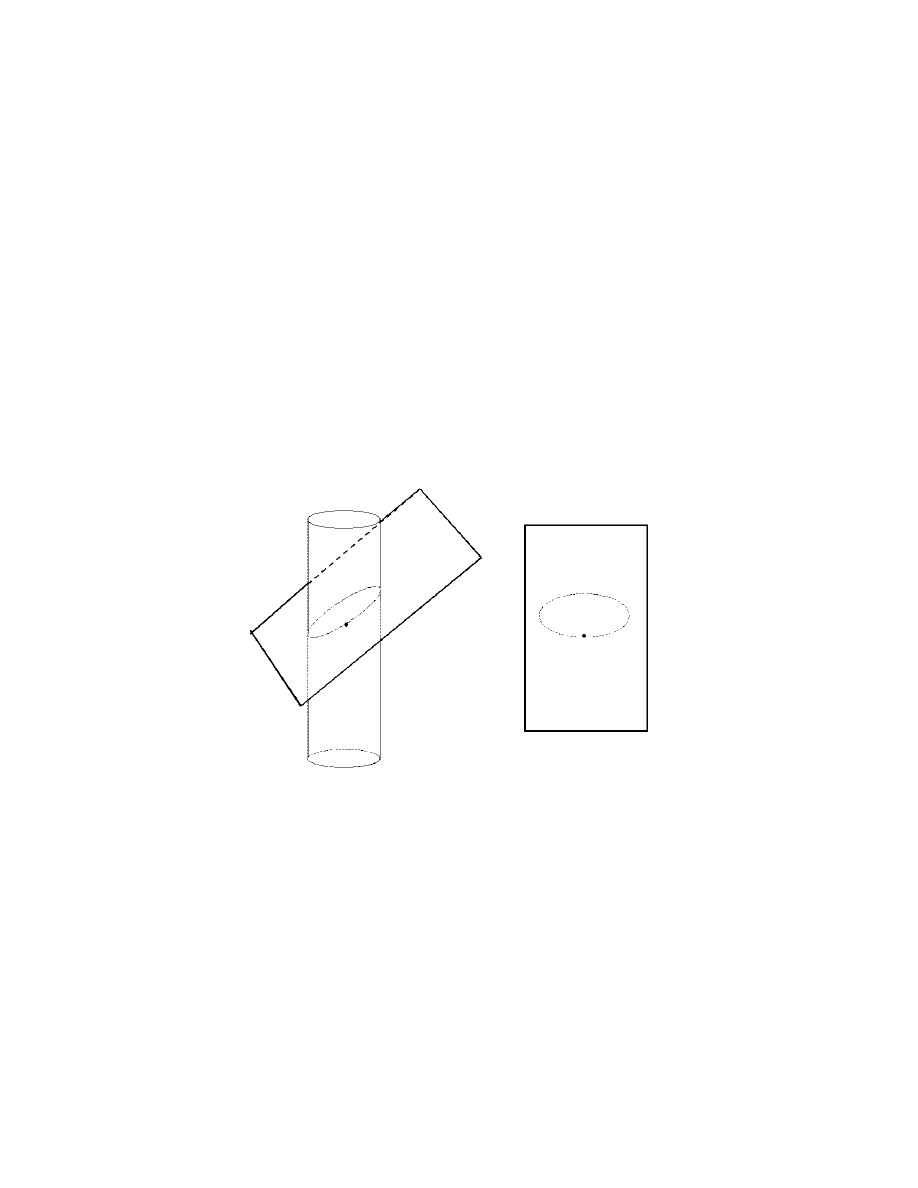
Definition. Let v be a unit vector tangent to a smooth surface M ⊂ E
3
at a point
P (again making no distinction between a vector and a point).
Let
U be a unit vector normal (perpendicular) to M at point P . The
plane through point
P which contains vectors v and U intersects the
surface in a curve α
v
called the normal section of M at
P in the direction
v. See Figure I-10.
Example. Find the normal section of M : x
2
+ y
2
= 1 (an infinitely
tall right circular cylinder of radius 1) at the point
P = (1, 0, 0) in the
direction v = (0, 1, 0).
1
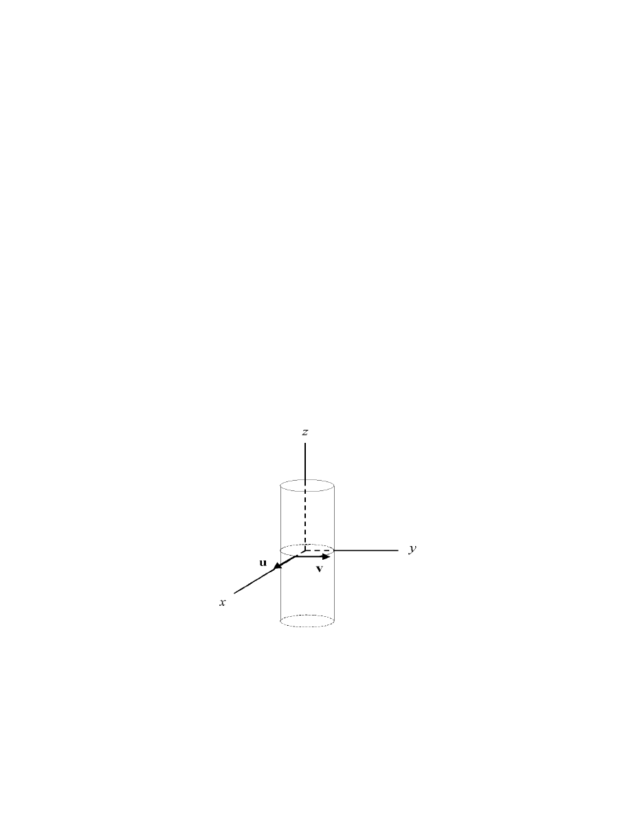
Solution. A normal vector to M at
P is
∇(x
2
+ y
2
) = (2x, 2y, 0)|
(1,0,0)
= (2, 0, 0).
Therefore, we take
U = (1, 0, 0). The plane containing U and v has as
a normal vector
U × v =
i j k
1 0 0
0 1 0
= (0, 0, 1).
Therefore the equation of this plane is
0(x − 1) + 0(y − 0) + 1(z − 0) = 0
or z = 0. The intersection of this plane and the surface is
α
v
= {(x, y, z) | x
2
+ y
2
= 1, z = 0}.
Note. Each normal vector α
v
to a surface can be approximated by
a circle (as in the previous section). Recall that if a plane curve has
a curvature k at some point
P , then this osculating circle has radius
2
1/k and its center is located 1/k units from
P in the direction of the
principal normal vector
N.
Definition. Let α
v
be a normal section to a smooth surface M at point
P in the direction v. Let U be a unit normal to M at P (−U is also
a unit normal to M at
P ). The normal curvature of M at P in the v
direction with respect to
U, denoted k
n,
U
(v), is
k
n,
U
(v) =
U · N
R(v)
where
N is the principal normal vector of α
v
at
P and R(v) is the
radius of the osculating circle to α
v
at
P . If α
v
has zero curvature at
P, we take k
n,
U
(v) = 0.
Note. If
U and
N are parallel, then
k
n,
U
(v) =
1
R(v)
and if
U and
N are antiparallel (i.e. point in opposite directions) then
k
n,
U
(v) =
−1
R(v)
.
So,
k
n,
U
(v)
is just the curvature of α
v
at
P . The text does not include
the vector
U in its notation, but our approach is equivalent to its.
Example. What is k
n,
U
(v) for the cylinder x
2
+ y
2
= 1 at
P = (1, 0, 0)
in the direction v = (0, 1, 0) with respect to
U = (1, 0, 0)?
Solution. As we saw in the previous example,
α
v
= {(x, y, z) | x
2
+ y
2
= 1, z = 0}.
3

We can parameterize α
v
as
α(s) = (cos s, sin s, 0)
where s ∈ [0, 2π]. Then
T(s) = α
(s) = (− sin s, cos s, 0)
and
T
(s) = α
(s) = (− cos s, − sin s, 0).
At point
P , s = 0, so the principal normal vector at P is
N(0) = T
(0)/
T
(0) = (−1, 0, 0).
Therefore
k
n,
U
(v) =
U · N
R(v)
=
−1
1
= −1.
Note. We will see in Section 6 that the normal curvature of M at
P in
the v direction with respect to
U assumes a maximum and a minimum
in directions v
1
and v
2
(respectively) which are orthogonal.
Definition. The directions v
1
and v
2
described above are the principal
directions of M at
P . Let k
1
and k
2
be the maximum and minimum
values (respectively) of k
n,
U
(v) at
P (we can take v = v
1
and v = v
2
,
respectively). Then k
1
and k
2
are the principal curvatures of M at
P .
The product k
1
k
2
is the Gauss curvature of M at
P , denoted K( P):
K( P) = k
1
k
2
.
Note. Even though k
n,
U
(v) depends on the choice of
U, K( P) is inde-
pendent of the choice of
U (if we use −U for the normal to the surface
4
instead of
U, we change the sign of k
n,
U
(v) and so the product k
1
k
2
remains the same).
Example. Evaluate K(
P) for the right circular cylinder x
2
+ y
2
= 1
at
P = (1, 0, 0).
Solution. At
P , α
v
is an ellipse with semi-minor axis 1, unless v =
(0, 0, ±1):
With
U = (1, 0, 0) (and
N = (−1, 0, 0) which implies nonpositive
k
n,
U
(v)) we have a minimum value of normal curvature of k
2
= −1
(as given in the previous example - this value is attained when α
v
is a
circle). Now with v = (0, 0, ±1) we get that α
v
is a pair of parallel lines
and then k
n,
U
(v) = 0 (recall the curvature of a line is 0). So
K( P) = (−1)(0) = 0.
5
Note. The Gauss curvature of a cylinder is 0 at every point. This
is also the case for a plane. An INFORMAL reason for this is that a
cylinder can be cut and peeled open to produce a plane (and conversley)
without stretching or tearing (other than the initial cut) and without
affecting lengths (such an operation is called an isometry).
Example. A sphere of radius r has normal curvature at every point
of k
n,
U
(v) = ±1/r (depending on the choice of
U) and so the Gauss
curvature is K = 1/r
2
.
Note. A surface M has positive curvature at point
P if, in a deleted
neighborhood of
P on M, all points lie on the same side of the plane
tangent to M at
P . If for all neighborhoods of P on M, some points
are on one side of the tangent plane and some points are on the other
side, then the surface has negative curvature (this will be made more
rigorous latter).
Example 5, p. 18. The hyperbolic paraboloid
z =
1
2
(y
2
− x
2
)
has negative curvature at each point.
Example 6, p. 19. A torus has some points with positive curvature,
some with negative curvature and some with 0 curvature.
Note. We have defined curvature as an extrinsic property of a surface
(using things external to the surface such as normal vectors). We will
6

see in Gauss’ Theorema Egregium that we can redefine curvature as
an intrinsic property which can be measured only using properties of
the surface itself and not using any properties of the space in which
the surface is embedded. This will be important when we address the
questions as to whether the universe is open or closed (and whether it
has positive, zero, or negative curvature).
7

1.3 Surfaces in E
3
Note. A surface M may be described as the image of a subset D of
R
2
under a vector valued function of two variables
X(u, v) = (x(u, v), y(u, v), z(u, v)).
When using this notation, we assume x, y, z have continuous partial
derivatives up to the third order.
Definition. A surface given as above is regular if the vectors
X
1
(u, v) =
∂
X
∂u
=
∂x
∂u
,
∂y
∂u
,
∂z
∂u
X
2
(u, v) =
∂
X
∂v
=
∂x
∂v
,
∂y
∂v
,
∂z
∂v
are linearly independent for each (u, v) ∈ D.
Note.
X
1
and
X
2
are linearly independent on D is equivalent to the
property:
X
1
×
X
2
= 0 for all (u, v) ∈ D.
Note. The condition of regularity insures that
X is one-to-one and has
a continuous inverse.
Example (Exercise 1.3.1(a)). If a smooth curve of the form α(u) =
(f (u), 0, g(u)) in the xz−plane is revolved about the z−axis, the re-
sulting surface of revolution is given by
X(u, v) = (f(u) cos v, f(u) sin v, g(u)).
1
Show that
X is regular provided f(u) = 0 and α
(u) = 0 for all u.
Solution. Well,
X
1
(u, v) =
∂
X
∂u
= (f
(u) cos v, f
(u) sin v, g
(u))
X
2
(u, v) =
∂
X
∂v
= (−f (u) sin v, f (u) cos v, 0).
If α
(u) = 0 for all u, then for a given u, either g
(u) = 0 or f
(u) = 0.
If g
(u) = 0 then
X
1
and
X
2
are linearly independent (in the third
component). If f
(u) = 0 and g
(u) = 0, consider:
X
1
×
X
2
= f
(u)f (u)(cos
2
v + sin
2
v)k = f
(u)f (u)k.
Since f (u) = 0 for all u, f
(u)f (u) = 0 and so
X
1
×
X
2
= 0 and
X
1
and
X
2
are linearly independent.
Definition. A vector v is a tangent vector to surface M at point
P if
there is a curve on M which passes through
P and has velocity vector
v at P. The set of all tangent vectors to M at P is the tangent plane
of M at
P , denoted T
P
M.
Note. T
P
M is a 2-dimensional vector space with {
X
1
(u
0
, v
0
),
X
2
(u
0
, v
0
)}
as a basis, where
X(u
0
, v
0
) =
P .
Definition. The curve
X(u, v
0
) is a u−parameter curve and
X(u
0
, v)
is a v−parameter curve of surface M (u
0
and v
0
are constants).
Note.
X
1
(u
0
, v
0
) is a velocity vector of
X(u, v
0
) and
X
2
(u
0
, v
0
) is a
velocity vector of
X(u
0
, v).
2

Example (Exercise 1.3.1(b)). Consider the surface of revolution
of Exercise 1.3.1(a). Describe the u− and v−parameter curves and
show they intersect orthogonally (the u−parameter curves are called
meridians and the v−parameter curves are called parallels).
Solution. A u−parameter curve is of the form (f (u) cos v
0
, f(u) sin v
0
,
g(u)) and has direction
X
1
(u, v
0
) = (f
(u) cos v
0
, f
(u) sin v
0
, g
(u)). A
v−parameter curve is of the form (f(u
0
) cos v, f (u
0
) sin v, g(u
0
)) and has
direction
X
2
(u
0
, v) = (−f(u
0
) sin v, f (u
0
) cos v, 0). If a u−parameter
curve and a v−paramter curve intersect at (u
0
, v
0
) then at this point
of intersection
X
1
(u
0
, v
0
) ·
X
2
(u
0
, v
0
) = −f (u
0
)f
(u
0
) cos v
0
sin v
0
+f (u
0
)f
(u
0
) cos v
0
sin v
0
+ g
(u
0
) × 0 = 0.
Therefore the u−parameter and v−parameter curves are orthogonal
when they intersect.
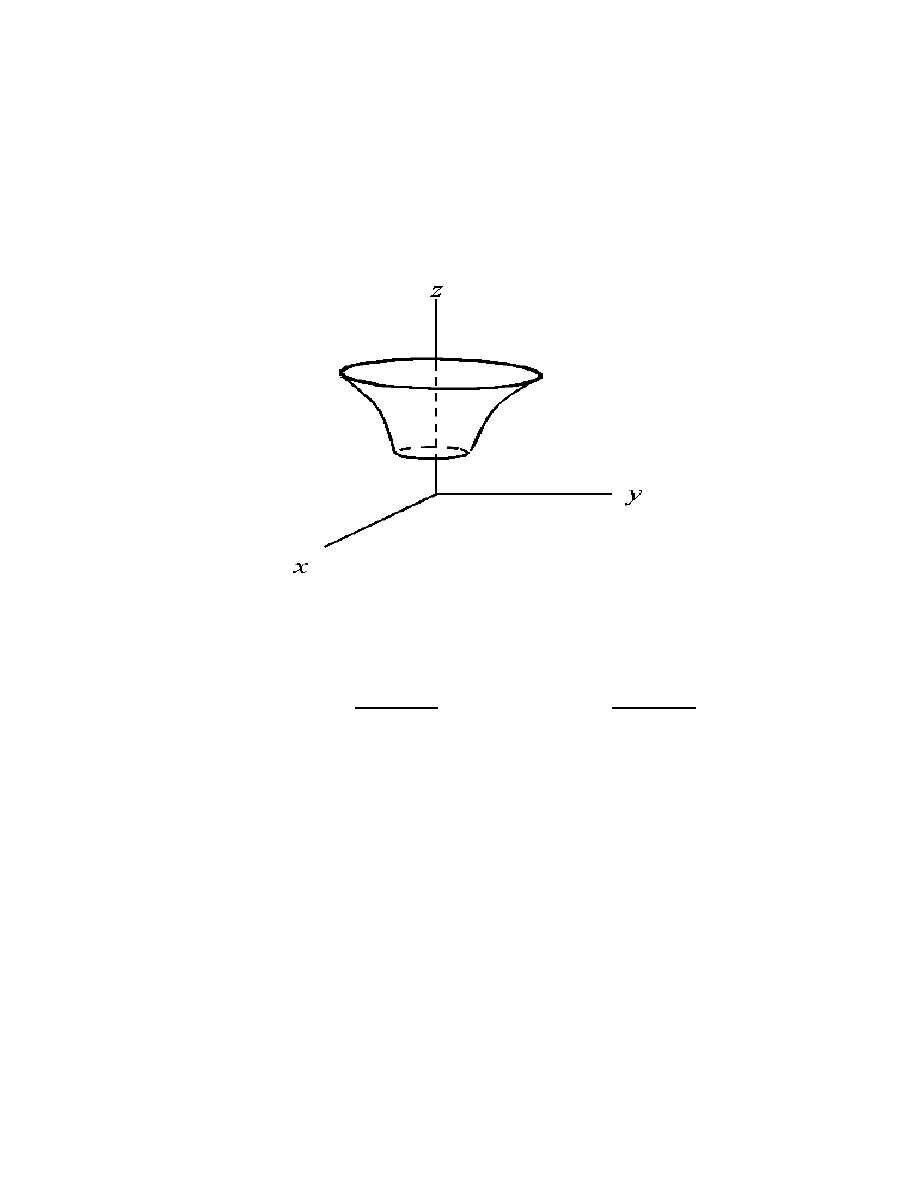
Example (Exercise 1.3.2(e)). For the surface of revolution
X(u, v) =
(a sinh u cos v, a sinh u sin v, b cosh u), u = 0, sketch the profile curve
(v = 0) in the xz−plane, and then sketch the surface. Prove that
X is
regular and give an equation for the surface of the form g(x, y, z) = 0.
Solution. For the profile, with v = 0 we have x = a sinh u and z =
b cosh u. Since cosh
2
u − sinh
2
u = 1, we have
z
b
2
−
x
a
2
= 1,
x = 0.
3
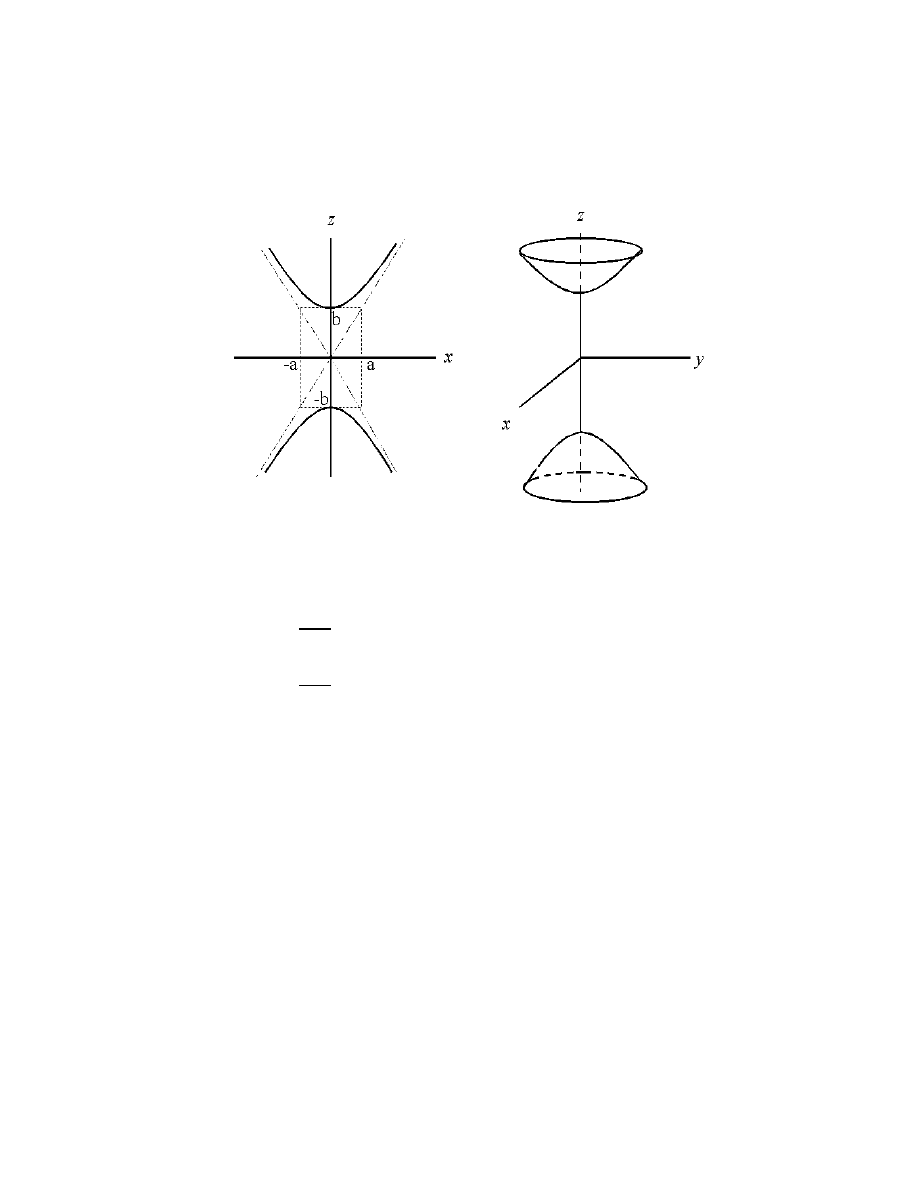
So the profile and surface are:
Next,
X
1
=
∂
X
∂u
= (a cosh u cos v, a cosh u sin v, b sinh u)
X
2
=
∂
X
∂v
= (−a sinh u sin v, a sinh u cos v, 0).
So
X
1
and
X
2
are linearly independent since b sinh u = 0 for u = 0.
Therefore
X is regular. Since
x = a sinh u cos v
y = a sinh u sin v
z = b cosh u
then g(x, y, z) = a
2
z
2
− (b
2
x
2
+ b
2
y
2
) − a
2
b
2
= 0 is the equation of the
surface.
4
1.4 The First Fundamental Form
Note. Suppose M is a surface determined by
X(u, v) ⊂ E
3
and
suppose α(t) is a curve on M, t ∈ [a, b]. Then we can write α(t) =
X(u(t), v(t)) (then (u(t), v(t)) is a curve in R
2
whose image under
X
is α). Then
α
(t) =
∂
X
∂u
du
dt
+
∂
X
∂v
dv
dt
= u
X
1
+ v
X
2
.
If s(t) represents the arc length along α (with s(a) = 0) then
s(t) =
t
a
α
(r)dr
and
ds
dt
= α
(t)
so
ds
dt
2
= α
(t)
2
= α
· α
= (u
X
1
+ v
X
2
) · (u
X
1
+ v
X
2
)
= u
2
(
X
1
·
X
1
) + 2u
v
(
X
1
·
X
2
) + v
2
(
X
2
·
X
2
).
Following Gauss’ notation (briefly) we denote
E =
X
1
·
X
1
,
F =
X
1
·
X
2
,
G =
X
2
·
X
2
and have
ds
dt
2
= E
du
dt
2
+ 2F
du
dt
dv
dt
+ G
dv
dt
2
or in differentialnotation
ds
2
= E(du)
2
+ 2F (du dv) + G(dv)
2
.
1
Definition. Let M be a surface determined by
X(u, v). The first
fundamental form (or more commonly metric form) of M is
ds
dt
2
or
(ds)
2
as defined above.
Definition. A property of a surface which depends only on the metric
form of the surface is an intrinsic property.
Note. The idea of an intrinsic property is that a “resident” of the sur-
face can detect such a property without appealling to a “larger space”
in which the surface is imbedded. Certainly an inhabitant of a surface
can measure distance within the surface.
Example 10, page 32. Consider the xy−plane described as
X(u, v) =
(u, v, 0) where u ∈ R and v ∈ R. Then
X
1
= (1, 0, 0) and
X
2
= (0, 1, 0).
So
E =
X
1
·
X
1
= 1,
F =
X
1
·
X
2
= 0,
G =
X
2
·
X
2
= 1.
Then the first fundamentalform is
ds
dt
2
=
du
dt
2
+
dv
dt
2
or, in terms of x and y:
ds
dt
2
=
dx
dt
2
+
dy
dt
2
.
Of course, this is the “usual” expression for the differential of arclength
from Calculus 2.
Definition. The matrix of the first fundamental form of a surface M
2

determined by
X(u, v) is
E F
F G
≡
g
11
g
12
g
21
g
22
where E, F , G are as defined as above.
Note. This matrix determines dot products of tangent vectors. If
v = a
X
1
+ b
X
2
and
w = c
X
1
+ d
X
2
are vectors tangent to a surface M
at a given point, then
v · w = (a
X
1
+ b
X
2
) · (c
X
1
+ d
X
2
) = Eac + F (ad + bc) + Gbd
= (a, b)
E F
F G
c
d
.
Notation. We now replace the parameters u and v with u
1
and u
2
.
We then have
ds
2
= g
11
(du
1
)
2
+ 2g
12
du
1
du
2
+ g
22
(du
2
)
2
=
i,j
g
ij
du
i
du
j
where the summation is taken (throughout this chapter) over the set
{1, 2}. In Chapter 3, we will sum over {1, 2, 3, 4}. If v is a vector
tangent to M at a point
P and v = (v
1
, v
2
) in the basis {
X
1
,
X
2
} for
the tangent plane at
P , then we have
v =
i
v
i
X
i
.
If α(t) is a curve on M where α is represented by
X(u
1
(t), u
2
(t)) then
α
(t) = u
1
(t)
X
1
+ u
2
(t)
X
2
=
i
u
i
X
i
.
3

Notation. We denote the ij entry of (g
ij
)
−1
as g
ij
. Therefore (g
ij
)(g
ij
) =
I and
j
g
ij
g
jk
= δ
k
i
(the ik entry of I) where
δ
k
i
=
1 if i = k
0 if i = k
.
Example (Exercise 1.4.3(c)). For the surface
X(u, v) = (u cos v, u sin v, bv)
(the helicoid of Example 9), compute the matrix (g
ij
), its determinate
g, the inverse matrix (g
ij
) and the unit normalvector
U.
Solution. Well
X
1
=
∂
X
∂u
= (cos v, sin v, 0)
X
2
=
∂
X
∂v
= (−u sin v, u cos v, b)
and so
g
11
=
X
1
·
X
1
= cos
2
v + sin
2
v + 0 = 1
g
22
=
X
2
·
X
2
= u
2
sin
2
v + u
2
cos
2
v + b
2
= u
2
+ b
2
g
12
=
X
1
·
X
2
= −u cos v sin v + u cos v sin v + 0 = 0 = g
21
.
Therefore
G =
g
11
g
12
g
21
g
22
=
1
0
0 u
2
+ b
2
and g = det(g
ij
) = u
2
+ b
2
. Then
G
−1
=
g
11
g
12
g
21
g
22
=
1
g
g
22
−g
12
−g
21
g
11
4
=
1
u
2
+ b
2
u
2
+ b
2
0
0
1
=
1
0
0
1
u
2
+b
2
.
Now the unit normalvector is
U =
X
1
×
X
2
X
1
×
X
2
and
X
1
×
X
2
=
i
j
k
cos v
sin v
0
−u sin v u cos v b
= (b sin v, −b cos v, u cos
2
v + u sin
2
v) = (b sin v, −b cos v, u).
Now
X
1
×
X
2
=
b
2
sin
2
v + b
2
cos
2
v + u
2
=
√
b
2
+ u
2
.
Therefore
U =
b sin v
√
b
2
+ u
2
,
−b cos v
√
b
2
+ u
2
,
u
√
b
2
+ u
2
.
Definition. Suppose Ω is a closed subset of the u
1
u
2
−plane and that
X : Ω → E
3
is smooth (i.e. has continuous first partials), is one-to-one
and regular (i.e.
X
1
and
X
2
are linearly independent) on the interior
of Ω. Then the area of the surface
X(Ω) is
A =
Ω
X
1
×
X
2
du
1
du
2
=
Ω
√
gdu
1
du
2
.
(See page 37 of the text for motivation of this definition.)
Example (Exercise 1.4.6). (a) Show that the area A of the surface
of revolution
X(u, v) = (f(u) cos v, f(u) sin v, g(u)) where u ∈ [a, b] and
v ∈ [0, 2π] is given by
A = 2π
b
a
|f(u)|
f
(u)
2
+ g
(u)
2
du.
5
(b) Show that the area of the surface obtained by revolving the graph
y = f(x) for x ∈ [a, b] about the x−axis is given by
A = 2π
b
a
|f(x)|
1 + f
(x)
2
dx.
Solution. (a) Consider the surface area of the surface of revolution
X(u, v) = (f(u) cos v, f(u) sin v, g(u)). We have (from Exercise 1.4.5)
X
1
×
X
2
= |f(u)|
f
(u)
2
+ g
(u)
2
and so
A =
Ω
X
1
×
X
2
du dv
(see page 37)
=
b
a
2π
0
|f(u)|
f
(u)
2
+ g
(u)
2
dv du
= 2π
b
a
|f(u)|
f
(u)
2
+ g
(u)
2
du.
(b) If y = f (x), x ∈ [a, b] where a ≥ 0 is revol ved about the x−axis,
then we have:
6
This is equivalent to taking
X(u, v) = (f(u), 0, u) (that is, the curve
x = f(z) in the xz−plane) and revolving it about the z−axis):
Then by Exercise 1.3.1, the surface is
X(u, v) = (f(u) cos v, f(u) sin v, u).
So by part (a), the surface area is
A = 2π
b
a
|f(u)|
f
(u) + 1 du = 2π
b
a
|f(x)|
f
(x) + 1 dx.
7
1.5 The Second Fundamental Form
Notation. We adopt the Einstein summation convention in which any
expression that has a single index appearing both as a subscript and a
superscript is assumed to be summed over that index.
Example. We denote
i
v
i
X
i
as v
i
X
i
.
Example. We denote
i,j
g
ij
v
i
w
j
as g
ij
v
i
w
j
.
Note. We have treated a path α(t) along a surface M as if it were the
trajectory of a particle in E
3
. We then interprete α
(t) as the accelera-
tion of the particle. Well, a particle can accelerate in two different ways:
(1) it can accelerate in the direction of travel, and (2) it can accelerate
by changing its direction of travel. We can therefore decompose α
into two components, α
T
(representing acceleration in the direction of
travel) and α
N
(representing acceleration that changes the direction of
travel). You may have dealt with this in Calculus 3 by taking α
T
as
the component of α
in the direction of α
(computed as
α
T
=
α
·
α
α
α
α
and α
N
as the “remaining component” of α (that is, α
N
= α
− α
T
).
This is reminiscent of the Frenet formulas or the Frenet frame (
T,
N, B)
of Exercise 1.1.14).
1
Note. With α parameterized in terms of arc length s, α = α(s) =
X(u
1
(s), u
2
(s)) we have the unit tangent vector
T (s) = α
(s) = u
i
X
i
.
We saw in Section 1.1 that α
(s) =
T
(s) is a vector normal to α
(
T
= k
N - see Exercise 1.1.14). In this section, we again decompose
α
into two orthogonal components, but this time we make explicit use
of the surface M. We wish to write
α
= α
tan + α
nor
where α
tan is the component of α
tangent to M and α
nor is the com-
ponent of α
normal to M. Notice that α
tan will be a linear combina-
tion of
X
1
and
X
2
(they are a basis for the tangent plane, recall) and
α
nor will be a multiple of the unit normal vector to M,
U (calculated
as
U =
X
1
×
X
2
X
1
×
X
2
).
Note. Since α(s) =
X(u
1
(s), u
2
(s)) and α
= u
i
X
i
(here, means
d/ds), then
α
= u
i
X
i
+ u
i
X
i
= u
i
X
i
+ u
i
d
X
i
ds
.
Now u
i
X
i
is part of α
tan, but u
i
X
i
may also have a component in the
tangent plane. Well,
d
X
i
ds
=
d
ds
X
i
(u
1
(s), u
2
(s))
=
∂
X
i
∂u
1
du
1
ds
+
∂
X
i
∂u
2
du
2
ds
=
∂
X
i
∂u
1
u
1
+
∂
X
i
∂u
2
u
2
=
∂
X
i
∂u
j
u
j
.
If we denote
∂
2
X
∂u
i
∂u
j
=
X
ij
(we have assumed continuous second par-
tials, so the order of differentiation doesn’t matter) then we have
d
X
i
ds
=
2
X
ij
u
j
. So acceleration becomes
α
= u
r
X
r
+ u
i
u
j
X
ij
.
We now need only to write
X
ij
in terms of a component in the tangent
plane (and so in terms of
X
1
and
X
2
) and a component normal to the
tangent plane (which will be a multiple of
U).
Definition. With the notation above, we define the formulae of Gauss
as
X
ij
= Γ
r
ij
X
r
+ L
ij
U.
That is we define L
ij
as the projection of
X
ij
in the direction
U. Notice,
however, that Γ
r
ij
may not be the projection of
X
ij
onto
X
r
since the
X
r
’s are not orthonormal.
Note. Since projections are computed from dot products, we immedi-
ately have that
L
ij
=
X
ij
· U =
X
ij
·
X
1
×
X
2
X
1
×
X
2
.
Note. We therefore have
α
= α
tan + α
nor =
u
r
+ Γ
r
ij
u
i
u
j
X
r
+
L
ij
u
i
u
j
U.
3
Definition. The second fundamental form of surface M is the matrix
L
11
L
12
L
21
L
22
.
(Notice this differs from the text’s definition on page 44.) We denote
the determinate of this matrix as L.
Note. The second fundamental form is a function of u and v. Also,
since we have
X
12
=
X
21
, it follows that L
12
= L
21
and so (L
ij
) is a
symmetric matrix.
Note. We will see that the second fundamental form reflects the ex-
trinsic geometry of surface M (that is, the way M is imbedded in E
3
-
“how it curves relative to that space” as the text says).
Example (Exercise 1.5.2). Compute the second fundamental form
of the surface of revolution
X(u, v) = (f(u) cos v, f(u) sin v, g(u)).
Solution. Well
X
1
=
∂
X
∂u
= (f
(u) cos v, f
(u) sin v, g
(u))
X
2
=
∂
X
∂v
= (−f (u) sin v, f (u) cos v, 0)
and so (from Exercise 1.4.5)
U =
f(u)
|f(u)|
f
(u)
2
+ g
(u)
2
(−g
(u) cos v, −g
(u) sin v, f
(u)).
4
Next,
X
11
=
∂
2
X
∂
2
u
= (f
(u) cos v, f
(u) sin v, g
(u))
X
22
=
∂
2
X
∂
2
v
= (−f (u) cos v, −f (u) sin v, 0)
X
12
=
∂
2
X
∂u∂v
= (−f
(u) sin v, f
(u) cos v, 0) =
X
21
.
So
L
11
=
X
11
· U =
f(u)
|f(u)|
f
(u)
2
+ g
(u)
2
(−f
(u)g
(u) cos
2
v
−f
(u)g
(u) sin
2
v + f
(u)g
(u))
=
f(u)(f
(u)g
(u) − f
(u)g
(u))
|f(u)|
f
(u)
2
+ g
(u)
2
L
12
=
X
12
· U =
(f (u)g
(u) cos v sin v − f (u)g
(u) cos v sin v + 0)f (u)
|f(u)|
f
(u)
2
+ g
(u)
2
= 0 = L
21
L
22
=
X
22
· U =
f(u)
|f(u)|
f
(u)
2
+ g
(u)
(f (u)g
(u) cos
2
v
+f (u)g
(u) sin
2
v + 0)
=
f(u)
2
g
(u)
|f(u)|
f
(u) + g
(u)
2
=
|f(u)|g
(u)
f
(u)
2
+ g
(u)
2
.
Therefore the Second Fundamental Form is
L = det L
ij
= L
11
L
22
− L
12
L
21
=
f(u)(f
(u)g
(u) − f
(u)g
(u))
|f(u)|
f
(u)
2
+ g
(u)
2
|f(u)|g
(u)
f
(u)
2
+ g
(u)
2
=
f(u)g
(u)(f
(u)g
(u) − f
(u)g
(u))
f
(u)
2
+ g
(u)
2
.
5
Definition. Let v = v
i
X
i
be a unit vector tangent to M at
P . The
normal curvature of
M at P in the direction v, denoted k
n
(v) is
k
n
(v) = L
ij
v
i
v
j
where v = (v
1
, v
2
).
Example (Exercise 1.5.5). Find the normal curvature of the surface
z = f(x, y) at an arbitrary point, in the direction of a unit tangent
vector (a, b, c) at that point.
Solution. We have
X
1
=
∂
X
∂u
= (1, 0,
∂f
∂u
(u, v)) = (1, 0, f
u
)
X
2
=
∂
X
∂v
= (0, 1,
∂f
∂v
(u, v)) = (0, 1, f
v
).
So
X
1
×
X
2
=
i j k
1 0 f
u
0 1 f
v
= (−f
u
, −f
v
, 1)
and
X
1
×
X
2
=
(f
u
)
2
+ (f
v
)
2
+ 1. Therefore
U =
X
1
×
X
2
X
1
×
X
2
=
1
(f
u
)
2
+ (f
v
)
2
+ 1
(−f
u
, −f
v
, 1).
Now
X
11
=
∂
2
X
∂u
2
= (0, 0, f
uu
)
X
12
=
∂
2
X
∂u ∂v
= (0, 0, f
uv
) =
X
21
X
22
=
∂
2
X
∂v
2
= (0, 0, f
vv
)
6
and so
L
11
=
X
11
· U =
f
uu
(f
u
)
2
+ (f
v
)
2
+ 1
L
22
=
X
22
· U =
f
vv
(f
u
)
2
+ (f
v
)
2
+ 1
L
12
=
X
12
· U =
f
uv
(f
u
)
2
+ (f
v
)
2
+ 1
= L
21
.
Now v = v
i
X
i
= v
1
(1, 0, f
u
) + v
2
(0, 1, f
v
) = (a, b, c), implying that
v
1
= a and v
2
= b. Hence
k
n
(v) = L
ij
v
i
v
j
= L
11
v
1
v
1
+ 2L
12
v
1
v
2
+ L
22
v
2
v
2
=
1
(f
u
)
2
+ (f
v
)
2
+ 1
(a
2
f
uu
+ 2abf
uv
+ b
2
f
vv
).
Note. If α =
X(u
1
(s), u
2
(s)) is a curve on M,
P is a point on M
with α(s
0
) =
P and v = α
(s
0
) then α
(s
0
) = u
i
(s
0
)
X
i
(u
1
(s
0
), u
2
(s
0
))
and so v
i
= u
i
(s
0
) (see page 35 for representation of a tangent vector:
v = v
i
X
i
). Therefore
k
n
(v) = L
ij
v
i
v
j
= L
ij
u
i
u
j
.
Now α
= u
r
X
r
+u
i
u
j
X
ij
(equation (16), page 43), and
U =
X
1
×
X
2
X
1
×
X
2
so
α
· U =
u
r
X
r
+ u
i
u
j
X
ij
·
X
1
×
X
2
X
1
×
X
2
= 0 + u
i
u
j
X
ij
·
X
1
×
X
2
X
1
×
X
2
= u
i
u
j
L
ij
.
Hence k
n
(v) = α
· U. This equation is used in Exercise 1.5.6.
7

1.6 The Gauss Curvature in Detail
Note. We have defined the normal curvature of a surface at a point
P
in the direction v: k
n
(v). Therefore, for a given point on a surface, there
are an infinite number of (not necessarily distinct) curvatures (one for
each “direction”). We can think of k
n
(v) as a function mapping the
vector space T
P
(M) (the plane tangent to surface M at point
P ) into
R. That is k
n
: T
P
(M) → R. We need v to be a unit vector, so the
domain of k
n
is {v ∈ T
P
(M) | v = 1}. Therefore, k
n
is a continuous
functions on a compact set and by the Extreme Value Theorem (for
metric spaces), k
n
assumes a maximum and a minimum value.
Definition. Let M be a surface and
P a point on the surface. Define
k
1
=max k
n
(v) and k
2
=min k
n
(v) where the maximum and minimum
are taken over the domain of k
n
. k
1
and k
2
are called the principal cur-
vatures of M at
P , and the corresponding directions are called principal
directions. The product K = K(P ) = k
1
k
2
is the Gauss curvature of
M at P .
Theorem I-5. The Gauss curvature at any point
P of a surface M is
K( P) = L/g where L =det(L
ij
) and g =det(g
ij
).
Proof. First, if v = v
i
X
i
then
v
2
=
v
1
X
1
+ v
2
X
2
·
v
1
X
1
+ v
2
X
2
= (v
1
)
2
X
1
·
X
1
+ 2(v
1
)(v
2
)
X
1
·
X
2
+ (v
2
)
2
X
2
·
X
2
1

= g
mn
v
m
v
n
(recall g
mn
=
X
m
·
X
n
, see page 35).
Therefore finding extrema of k
n
(v) for v =1 is equivalent to finding
extrema of
k = k
n
(v) =
L
ij
v
i
v
j
g
mn
v
m
v
n
for v ∈ T
P
(M) and v = 0. If k
n
(v) is an extreme value of k, where
v = v
i
X
i
, then
∂k
∂v
1
=
∂k
∂v
2
= 0 at v (that is, the gradient of k is 0 -
however, this gradient is computed in a (v
1
, v
2
) coordinate system, not
(x, y)). Now
∂k
∂v
r
=
[2L
rj
v
j
](g
mn
v
m
v
n
) − (L
ij
v
i
v
j
)[2g
rn
v
n
]
(g
mn
v
m
v
n
)
2
for r = 1, 2 (the derivatives in the numerator follow from Exercise
1.5.1). Now k =
L
ij
v
i
v
j
g
mn
v
m
v
n
, so replacing L
ij
v
i
v
j
with kg
mn
v
m
v
n
gives
∂k
∂v
r
=
2L
rj
v
j
(g
mn
v
m
v
n
) − (kg
mn
v
m
v
n
)2g
rn
v
n
(g
mn
v
m
v
n
)
2
=
2L
rj
v
j
− 2kg
rn
v
n
g
mn
v
m
v
n
=
2L
rj
v
j
− 2kg
rj
v
j
g
mn
v
m
v
n
=
2(L
rj
− kg
rj
)v
j
g
mn
v
m
v
n
,
for r = 1, 2. So at an extreme value, (L
ij
−kg
ij
)v
j
= 0 for i = 1, 2. This
is two linear equations in two unknowns (v
1
and v
2
). Since v is nonzero,
the only way this system can have a solution is for det(L
ij
− kg
ij
) = 0.
That is
det
L
11
− kg
11
L
12
− kg
12
L
21
− kg
21
L
22
− kg
22
= 0
or (L
11
− kg
11
)(L
22
− kg
22
) − (L
21
− kg
21
)(L
12
− kg
12
) = 0
2
or L
11
L
22
− kL
11
g
22
− kL
22
g
11
+ k
2
g
11
g
22
−L
21
L
12
+ kL
21
g
12
+ kL
12
g
21
− k
2
g
12
g
21
= 0
or k
2
(g
11
g
22
− g
12
g
21
) − k(g
11
L
22
+ g
22
L
11
−g
12
L
12
− g
21
L
21
) + (L
11
L
22
− L
21
L
12
) = 0
or k
2
g − k(g
11
L
22
+ g
22
L
11
− 2g
12
L
12
) + L = 0
since L
12
= L
21
, L =det(L
ij
), and g =det(g
ij
). So for extrema of k we
need
k
2
− k
g
11
L
22
+ g
22
L
11
− 2g
12
L
12
g
+
L
g
= 0.
Since k
1
and k
2
are known to be roots of this equation, this equation
factors as (k − k
1
)(k − k
2
) = k
2
− (k
1
+ k
2
)k + k
1
k
2
= 0. Therefore, the
Gauss curvature is k
1
k
2
= L/g.
Note. L is the Second Fundamental form and g is the determinate
of the First Fundamental Form. We now see good evidence for these
being called “Fundamental” forms.
Example (Example 14, page 45 and Example 16, page 51).
Consider the surface
X(u, v) = (u, v, f(u, v)). Then
X
1
=(1, 0, f
u
),
X
2
=(0, 1, f
v
),
X
11
=(0, 0, f
uu
),
X
22
=(0, 0, f
vv
), and
X
12
=
X
21
=
(0, 0, f
uv
). With g
ij
=
X
i
·
X
j
we have
(g
ij
) =
1 + f
2
u
f
u
f
v
f
u
f
v
1 + f
2
v
3
and so g =det(g
ij
) = 1 + f
2
u
+ f
2
v
. Now
X
1
×
X
2
=
i j k
1 0 f
u
0 1 f
v
= (−f
u
, −f
v
, 1)
and
U =
X
1
×
X
2
X
1
×
X
2
=
X
1
×
X
2
√g =
1
√g(−f
u
, −f
v
, 1).
Next, L
ij
=
X
ij
· U, so
L
11
=
1
√gf
uu
L
12
=
1
√gf
uv
L
21
=
1
√gf
uv
L
22
=
1
√gf
vv
.
Therefore L =det(L
ij
) =
1
g
(f
uu
f
vv
− (f
uv
)
2
). So the Gauss Curvature
is
L
g
=
f
uu
f
vv
− (f
uv
)
2
g
2
=
f
uu
f
vv
− (f
uv
)
2
(1 + f
2
u
+ f
2
v
)
2
.
Note. You may recall from Calculus 3 that a critical point of z =
f(x, y) was tested to see if it was a local maximum or minimum by
considering D = f
xx
f
yy
− (f
xy
)
2
at the critical point. If D < 0, the
surface has a saddle point. If D > 0 and f
xx
> 0, it has a local
minimum. If D > 0 and f
xx
< 0, it has a local maximum. This all
makes sense now in the light of curvature!
Theorem. If v and
w are principal directions for surface M at point
P corresponding to k
1
(maximum normal curvature at
P ) and k
2
(min-
imum normal curvature at
P ) respectively, then if k
1
= k
2
we have v
and
w orthogonal.
4

Proof. Let v = v
i
X
i
and
w = w
i
X
i
. As in Theorem I-5 (equation (24),
page 50)
(L
ij
− k
1
g
ij
)v
j
= 0 for i = 1, 2, and
(L
ij
− k
2
g
ij
)w
j
= 0 for i = 1, 2.
The first of these equations is equivalent to
L
ij
v
i
= k
1
g
ji
v
i
for j = 1, 2
and since L
ij
= L
ji
and g
ij
= g
ji
to
L
ij
v
i
= k
1
g
ij
v
i
for j = 1, 2.
(25)
The second of these equations implies
(L
ij
− k
2
g
ij
)v
i
w
j
= 0
(we now sum over i = 1, 2). So
(L
ij
v
i
− k
2
g
ij
v
i
)w
j
= 0
and from (25) we have
(k
1
g
ij
v
i
− k
2
g
ij
v
i
)w
j
= 0
or
(k
1
− k
2
)g
ij
v
i
w
j
= 0.
Now v ·
w = g
ij
v
i
w
j
(see page 35). Since k
1
− k
2
=0, it must be that
v · w =0.
Note. We are now justified in refering to “two” principal directions.
When we consider the Gauss curvature at a point, we deal with the
5

normal curvature k
n
(v) at this point, where v = v
i
X
i
(i takes on the
values 1 and 2). So our collection of directions is a two dimensional
space. Since we have shown (for k
1
= k
2
) that the direction in which
k
n
(v) equals k
1
and the direction in which k
n
(v) equals k
2
are orthogo-
nal, there can be ONLY ONE direction in which k
n
(v) equals k
1
(well,
. . . plus or minus) and similarly for k
2
. In the event that k
1
= k
2
, we
choose two directions v and
w as principal directions where v · w = 0.
Definition. Suppose
P =
X(u
1
0
, u
2
0
) and let Ω be a neighborhood
of (u
1
0
, u
2
0
) on which
X is one-to-one with a continuous inverse
X
−1
:
X(Ω) → Ω. Define U(u
1
, u
2
) to be a unit normal vector to the surface
M determined by
X at point
X(u
1
, u
2
) (recall that
U =
X
1
×
X
2
/
X
1
×
X
2
). Therefore U :
X(Ω) → S
2
.
U is called the sphere mapping or
Gauss mapping of
X(Ω). The image of
X(Ω) under U (a subset of S
2
)
is the spherical normal image of
X(Ω).
Example (Exercise 9 (d), page 57). The spherical normal image
of a torus (see Example 12, page 34) is the whole sphere S
2
(there is a
normal vector pointing in any direction - in fact, the sphere mapping
is two-to-one).
Lemma I-6.
U
1
× U
2
= K(
X
1
×
X
2
).
Proof. Define L
i
j
= L
i
j
(u
1
, u
2
) = L
jk
g
ki
for i, j = 1, 2. Notice
L
i
j
g
im
= (L
jk
g
ki
)g
im
= L
jk
δ
k
m
= L
jm
(recall (g
ij
) is the inverse of (g
ij
)). Since
U · U =1, U · U
j
=0 (product
6

rule) and so
U
j
is tangent to M. Therefore
U
j
is a linear combination
of
X
1
and
X
2
:
U
j
= a
r
j
X
r
for j = 1, 2
for some coefficients a
r
j
. Since
U is normal to M and
X
k
is tangent to
M (at a given point) then U ·
X
k
=0. Differentiating this equation with
respect to u
j
gives
U
j
·
X
k
+
U ·
X
jk
= 0 and so
U
j
·
X
k
= −
U ·
X
jk
= −L
jk
(this last equality follows from equation (2), page 44). So
−L
jk
=
U
j
·
X
k
= a
r
j
X
r
·
X
k
= a
r
j
g
rk
,
for j, k = 1, 2 (recall the definition of g
rk
). We now solve these four
equations (j, k = 1, 2) in the four unknowns a
r
j
:
−L
jk
= a
r
j
g
rk
(j, k = 1, 2)
−g
ki
L
jk
= a
r
j
g
rk
g
ki
= a
r
j
δ
i
r
= a
i
j
(i, j = 1, 2).
Therefore (by the definition of L
i
j
) a
i
j
= −L
i
j
. We now see how U
i
and
X
j
relate:
U
j
= −L
i
j
X
i
for j = 1, 2.
From these relationships:
U
1
× U
2
= (−L
i
1
X
i
) × (−L
k
2
X
k
)
= (−L
1
1
X
1
− L
2
1
X
2
) × (−L
1
2
X
1
− L
2
2
X
2
)
= (L
1
1
L
2
2
− L
2
1
L
1
2
)
X
1
×
X
2
(recall v × v =0)
=det(L
i
j
)
X
1
×
X
2
.
Since L
i
j
= L
jk
g
ki
, then det(L
i
j
) = det(L
jk
) det(g
ki
) and since (g
ki
) is
the inverse of (g
ki
),
det(g
ki
) =
1
det(g
ki
)
=
1
g
7
and so
det(L
i
j
) =
det(L
jk
)
det(g
ki
)
=
L
g
= K.
Therefore,
U
1
× U
2
= K(
X
1
×
X
2
).
Definition. For a surface determined by
X(u
1
, u
2
), with
U
j
,
X
i
and
L
i
j
defined as above, the equations
U
j
= −L
i
j
X
i
for j = 1, 2 are the
equations of Weingarten.
Note. For Ω a neigborhood of (u
1
0
, u
2
0
) on which
X is one-to-one with
a continuous inverse, the set
X(Ω) is a connected region on M. The
spherical normal image of
X(Ω), U(Ω) is a region on S
2
(see Figure
I-26, page 52). If the curvature of
X(Ω) varies little then the area of
U(Ω) will be small. In fact, if X(Ω) is part of a plane, then the area of
U(Ω) is zero. In fact, for Ω small, the ratio of the area of U(Ω) to the
area of
X(Ω) approximates the curvature of M on Ω.
Note. The tangent plane to S
2
at
U(u
1
, u
2
), T
U
S
2
, is parallel (that is,
has the same normal vector) to the tangent plane to M at
X(u
1
, u
2
),
T
X
M. If U
1
× U
2
= 0 (i.e. if U
1
and
U
2
are linearly independent)
then
U
1
× U
2
U
1
× U
2
and
U are both unit normal vectors to S
2
at the point
U and do can differ at most in sign. That is, U = ±
U
1
× U
2
U
1
× U
2
or
U
1
× U
2
= ±
UU
1
× U
2
or U · U
1
× U
2
= ±
U
1
× U
2
(recall U · U =1).
Note. If (
U
1
× U
2
)(u
1
0
, u
2
0
) = 0 then
U is regular at (u
1
0
, u
2
0
) (by defini-
tion) and therefore (by the comment on page 24)
U is one-to-one with
8
a continuous inverse on sufficiently small Ω, a neighborhood of (u
1
0
, u
2
0
).
Also, with Ω sufficiently small,
U · U
1
× U
2
will be the same multiple of
U
1
× U
2
(namely +1 or −1). By equation (13), page 37,
Area U(Ω) =
Ω
U
1
× U
2
du
1
du
2
Area
X(Ω) =
Ω
X
1
×
X
2
du
1
du
2
.
Now
U · X
1
×
X
2
=
X
1
×
X
2
X
1
×
X
2
· (
X
1
×
X
2
) =
X
1
×
X
2
2
X
1
×
X
2
=
X
1
×
X
2
.
Also, we refer to
Ω
U · U
1
× U
2
du
1
du
2
as the signed area of
U(Ω)
(recall it is ±area of
U(Ω)). Therefore
signed area
U(Ω) =
Ω
U · U
1
× U
2
du
1
du
2
area
X(Ω) =
Ω
U · X
1
×
X
2
du
1
du
2
.
Note. If (
U
1
× U
2
)(u
1
0
, u
2
0
) = 0, then notice that
U · U
1
× U
2
may change
sign and
U may not be one-to-one over Ω and
Ω
U · U
1
× U
2
du
1
du
2
then represents a “net area” of
U(Ω). In all these cases, we denote
Ω
U · U
1
× U
2
du
1
du
2
as “Area
U(Ω)” even though this is a bit of a misnomer.
Theorem. Suppose M is a surface determined by
X(u
1
, u
2
) and
P =
X(u
1
0
, u
2
0
) is a point on M. Let Ω be a neighborhood of (u
1
0
, u
2
0
) on which
9
X is one-to-one with continuous inverse. Let U(Ω) be the spherical
normal image of
X(Ω). Then
K(P ) =lim
Ω→(u
1
0
,u
2
0
)
Area
U(Ω)
Area
X(Ω)
.
Here “Area
U(Ω)” is as discussed above. The limit is taken in the sense
that
sup{ dist (ω, (u
1
0
, u
2
0
)) | ω ∈ Ω}
approaches zero.
Proof. Let ! > 0. Then there exists δ
1
> 0 such that for Ω a ball with
center (u
1
0
, u
2
0
) and radius δ
1
we have
Area
U(Ω) − (U · U
1
× U
2
)(
P) Area(Ω)
=
Ω
U · U
1
× U
2
du
1
du
2
− (U · U
1
× U
2
)(
P ) Area(Ω)
< !
(since
U · U
1
× U
2
is continuous and Ω is connected). A similar result
holds for Area
X(Ω). Therefore, for Ω sufficiently small,
Area
U(Ω)
Area
X(Ω)
−
U · U
1
× U
2
U · X
1
×
X
2
(
P )
< !.
That is,
lim
Ω→(u
1
0
,u
2
0
)
Area
U(Ω)
Area
X(Ω)
=
U · U
1
× U
2
U · X
1
×
X
2
.
By Lemma I-6,
U · U
1
× U
2
U · X
1
×
X
2
=
U · K( X
1
×
X
2
)
U · X
1
×
X
2
= K
and the result follows.
10
Example (Exercise 8 (a), page 56). Let
X =
X(u, v) where (u, v) ∈
D be a parameterization of a surface M. The (signed) area of the
spherical normal image of M,
D
U · U
1
× U
2
du dv, is called the total
curvature of M (assuming the integral, which may be improper, exists).
Show that the total curvature of M is
D
K
√
g du dv (remember, K
and g are functions of u and v).
Solution. By Lemma I-6,
U
1
× U
2
= K(
X
1
×
X
2
). Therefore
U · U
1
× U
2
=
U · K(
X
1
×
X
2
).
Now the unit normal vector is
U =
X
1
×
X
2
X
1
×
X
2
, so
U · U
1
× U
2
=
K(
X
1
×
X
2
) · (
X
1
×
X
2
)
X
1
×
X
2
= K
X
1
×
X
2
.
By equation (10), page 35,
√g = X
1
×
X
2
. Therefore
U · U
1
× U
2
= K
√
g
and the total curvature of M over D is
D
U · U
1
× U
2
du dv =
D
K
√
g du dv.
Example (Exercise 9 (d), page 57). Compute the total curvature
of the torus
X(u, v) = ((R + r cos u) cos v, (R + r cos u) sin v, r sin u).
11
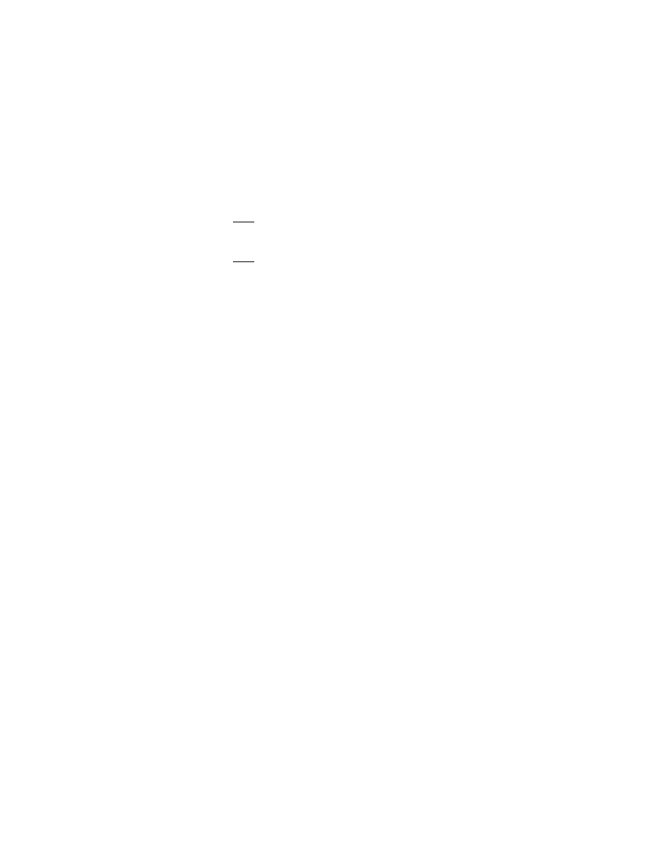
Solution. From Example 12, page 34, and Exercise 1.4.3 (d), page 38,
U = (− cos u cos v, − cos u sin v, − sin u).
So
U
1
=
∂ U
∂u
=(sin u cos v, sin u sin v, − cos u)
U
2
=
∂ U
∂v
=(cos u sin v, − cos u cos v, 0).
Therefore
U
1
× U
2
= (− cos
2
u cos v, − cos
2
u sin v, − sin u cos u cos
2
v
− sin u cos u sin
2
v)
= (− cos
2
u cos v, − cos
2
u sin v, − sin u cos u)
and
U · U
1
× U
2
=cos
3
u cos
2
v + cos
3
u sin
2
v + sin
2
u cos u
=cos
3
u + sin
2
u cos u.
So the total curvature is
π
−π
π
−π
(cos
3
u + sin
2
u cos u) du dv.
Now cos
3
u+sin
2
u cos u is an even function, so the integral is 0 and the
total curvature is 0.
12
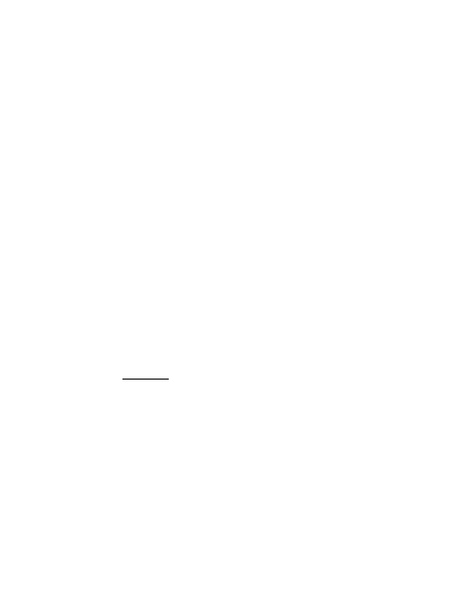
1.7 Geodesics
Note. A curve α(s) on a surface M can curve in two different ways.
First, α can bend along with surface M (the “normal curvature” dis-
cussed above). Second, α can bend within the surface M (the “geodesic
curvature” to be defined).
Recall. For curve α on surface M, α
can be written as components
tangent and normal to M as α
= α
tan + α
nor where
α
tan = (u
r
+ Γ
r
ij
u
i
u
j
)
X
r
α
nor = (L
ij
u
i
u
j
)
U
and the parameters on the right hand side are defined in Section 5.
α
nor reflects the curvature of α due to the bending of M and α
tan
reflects the curvature of α within M. Now
α
tan ·
U =
(u
r
+ Γ
r
ij
u
i
u
j
)
X
r
· U = 0
(recall
U =
X
1
×
X
2
X ×
X
2
) and
α
tan · α
= α
tan · α
+ 0 = α
tan · α
+ α
nor · α
(recall α
= u
i
X
i
and
X
i
· U = 0)
= (α
tan + α
nor) · α
= α
· α
= 0
(recall α
= α
(s) = 1 and = d/ds).
Therefore α
tan is orthogonal to both
U and α
. If we defi ne
w as the
unit vector
w = U × α
, then α
tan is a multiple of
w (and w is a vector
tangent to M).
1
Definition I-7. Let α(s) be a curve on M where s is arc length. The
geodesic curvature of α at α(s) is the function k
g
= k
g
(s) defi ned by
α
tan = k
g
w = k
g
(
U × α
).
Recall. The scalar triple product of three vectors (in R
3
) satisfies:
(
A × B) · C = ( B × C) ·
A = ( C ×
A) · B.
Theorem. The geodesic curvature k
g
of curve α in surface M can be
calculated as
k
g
=
U · α
× α
.
Proof. Since k
g
w = α
tan we have
k
g
w · w = α
tan ·
w = α
tan · (
U × α
)
or
k
g
= (α
tan + α
nor) ·
U × α
(since α
nor is parallel to
U)
= α
· U × α
=
U · α
× α
.
Definition I-8. Let α = α(s) be a curve on a surface M. Then α is a
geodesic if α
tan =
0 ( or equivalently, if α
= α
nor) at every point of
α.
2

Note. A geodesic on a surface is, in a sense, as “straight” as a curve
can be on the surface. That is, α has no curvature within the surface.
For example, on a sphere the geodesics are great circles.
Note. If α is a geodesic on M then
u
r
+ Γ
r
ij
u
i
u
j
= 0
for r = 1, 2 and
U · α
× α
= 0.
(We’ll use these LOTS!)
Example (Exercise 1.7.4(a)). Prove that on a surface of revolution,
every meridian is a geodesic.
Proof. Suppose
X(u, v) = (f(u) cos v, f(u) sin v, g(u)).
Let
m(s) = (f(s) cos v, f(s) sin v, g(s)) be a meridian of the surface
(where we assume the curve has been parameterized in terms of ar-
clength s). Then
m
(s) = (f
(s) cos v, f
(s) sin v, g
(s))
m
= (f
(s) cos v, f
(s) sin v, g
(s))
m
× m
= ((f
(s)g
(s) − f
(s)g
(s)) sin v, (−f
(s)g
(s) + f
(s)g
(s)) cos v, 0).
Now
X
1
×
X
2
= (−f (s)g
(s) cos v, −f (s)g
(s) sin v, f
(s)f (s))
3

and so
U =
X
1
×
X
2
X
1
×
X
2
=
(−f (s)g
(s) cos v, −f (s)g
(s) sin v, f
(s)f (s))
(f (s)g
(s))
2
+ (f
(s)f (s))
2
.
Therefore
U · m
× m
=
1
(f (s))
2
{(g
(s))
2
+ (f
(s))
2
}
×{(f
(s)g
(s) − f
(s)g
(s))(−f (s)g
(s)) cos v sin v
+(−f
(s)g
(s) + f
(s)g
(s))(−f (s)g
(s)) cos v sin v, 0)}
=
1
(f (s))
2
{(g
(s))
2
+ (f
(s))
2
}
(0) = 0.
Therefore
m(s) is a geodesic.
Definition. Let
X(u
1
, u
2
) be a surface and let g
ij
(see page 34) and
Γ
r
ij
(see page 43) be as defined in Sections 4 and 5. The Christoffel
symbols of the first kind are
Γ
ijk
= Γ
r
ij
g
rk
for i, j, k = 1, 2.
Definition. The Γ
r
ij
defined in Section 1.5 are the Cristoffel symbols
of the second kind.
Note. Since Γ
r
ij
= Γ
r
ji
(see (17), page 43) then Γ
ijk
= Γ
jik
. Also, since
(g
ij
)
−1
= (g
ij
), we have Γ
m
ij
= Γ
ijk
g
km
.
4
Theorem. Let
X(u
1
, u
2
) be a surface and let g
ij
and Γ
r
ij
be as defined
in Sections 4 and 5. Then
Γ
ijk
=
X
ij
·
X
k
Γ
ijk
=
1
2
∂g
ik
∂u
j
+
∂g
jk
∂u
i
−
∂g
ij
∂u
k
and
Γ
r
ij
=
1
2
g
kr
∂g
ik
∂u
j
+
∂g
jk
∂u
i
−
∂g
ij
∂u
k
.
Proof. Since
X
ij
= Γ
r
ij
X
r
+ L
ij
U (by definition, see page 43) then
X
ij
·
X
k
= Γ
r
ij
X
r
·
X
k
+ (L
ij
U) · X
k
= Γ
r
ij
g
rk
+ 0 = Γ
ijk
establishing the first identity (recall g
rk
=
X
r
·
X
k
). Next,
∂g
ik
∂u
j
=
∂
∂u
j
[
X
i
·
X
k
] =
X
ij
·
X
k
+
X
kj
·
X
i
= Γ
ijk
+ Γ
kji
.
Permuting the indices:
∂g
ji
∂u
k
= Γ
jki
+ Γ
ikj
and
∂g
kj
∂u
i
= Γ
kij
+ Γ
jik
.
Now
Γ
ijk
=
1
2
(2Γ
ijk
) =
1
2
(Γ
ijk
+ Γ
jik
)
=
1
2
(Γ
ijk
+ Γ
kji
− Γ
kji
+ Γ
kij
− Γ
kij
+ Γ
jik
)
=
1
2
{(Γ
ijk
+ Γ
kji
) + (Γ
kij
+ Γ
jik
) − (Γ
jki
+ Γ
ikj
)}
=
1
2
∂g
ik
∂u
j
+
∂g
jk
∂u
j
−
∂g
ij
∂u
k
and the second identity is established. Finally, multiplying this identity
on both sides by g
kr
, summing over k and using the definition of Γ
r
ij
we
5
have
Γ
r
ij
= Γ
ijk
g
kr
=
1
2
g
kr
∂g
ik
∂u
j
+
∂g
jk
∂u
j
−
∂g
ij
∂u
k
(recall (g
ij
= (g
ij
)
−1
), and the third identity is established.
Note. Since the Christoffel symbols depend only on the metric form
(or First Fundamental Form), they are part of the intrinsic geometry
of the surface M.
Definition. Let
X(u
1
, u
2
) be a surface. Then the coordinates
X
1
and
X
2
are orthogonal if g
12
= g
21
= 0. (This makes sense since g
ij
=
X
i
·
X
j
.)
Corollary. Let
X(u
1
, u
2
) be a surface and let g
ij
and Γ
r
ij
be as defined
in Sections 4 and 5. If
X
1
and
X
2
are orthogonal coordinates, then
Γ
r
ij
=
1
2g
rr
∂g
ir
∂u
j
+
∂g
jr
∂u
i
−
∂g
ij
∂u
r
(no sums over any of i, j, r).
Proof. Since g
12
= g
21
= 0, then g
12
= g
21
= 0 and g
11
= 1/g
11
,
g
22
= 1/g
22
. The result follows from the above theorem.
Corollary. With the hypotheses of the previous corollary (with i, j, r =
1, 2), when j = r
Γ
r
ir
=
1
2g
rr
∂g
rr
∂u
i
=
1
2
∂
∂u
i
[ln g
rr
]
and when i = j = r
Γ
r
ii
=
1
2g
rr
−
∂g
ii
∂u
r
.
6
Proof. Follows from g
12
= g
21
= 0.
Note. By symmetry, Γ
r
ij
= Γ
r
ji
, and so the previous two corollaries
cover all possible cases when i, j, r ∈ {1, 2} (i.e. when we deal with
two dimensions). In dimensions 3 and greater (in particular, in the 4
dimensional spacetime of Chapter III) we have a third case which we
state now, and address in detail later:
Theorem. In dimensions 3 and greater, if coordinates are mutually
orthogonal, then for i, j, r all distinct, Γ
r
ij
= 0. (In the event that one
or more of i, j, r are equal, the above corollaries apply.)
Note. In the case of orthogonal coordinates, if we return to Gauss’
notation:
g
11
= E,
g
12
= g
21
= F = 0,
g
22
= G
we have the First Fundamental Form (or metric form) ds
2
= Edu
2
+
Gdv
2
on surface
X(u, v). In this notation, the Christoffel symbols are
then
Γ
1
11
=
E
u
2E
Γ
2
22
=
G
v
2G
Γ
1
12
= Γ
1
21
=
E
v
2E
Γ
2
21
= Γ
2
12
=
G
u
2G
Γ
1
22
= −
G
u
2E
Γ
2
11
= −
E
v
2G
.
Example 17, page 62. In the Euclidean plane, ds
2
= du
2
+ dv
2
.
Therefore E = G = 1 and all the Christoffel symbols are 0. Therefore
7

a geodesic α satisfies
u
r
+ Γ
r
ij
u
i
u
j
= 0
for r = 1, 2, or u
r
= 0 for r = 1, 2. That is, u
1
= u
= 0 and
u
2
= v
= 0. Therefore u(s) = as + b and v(s) = cs + d for some
a, b, c, d. Therefore, geodesics in the Euclidean plane are straight lines.
Note. We will show in Theorem I-9 that the shortest path on a surface
joining two points is a geodesic. This theorem, combined with the pre-
vious example PROVES that the shortest distance between two points
in a plane is a straight line. Oddly enough, you’ve probably never seen
this PROVEN before!
Example 18, page 62. Consider a sphere of radius r with “geographic
coordinates” (like latitude and longitude) u and v. Then the sphere is
given by
X(u, v) = (r cos u cos v, r sin u cos v, r sin v)
(see Example 7, page 23). The metric form is (see page 33) ds
2
=
r
2
cos
2
vdu
2
+ r
2
dv
2
(since there is no du dv term, F = g
12
= g
21
= 0
and these coordinates are orthogonal). Therefore E = r
2
cos
2
v and
G = r
2
(a constant). Then E
u
= G
u
= G
v
= 0 and the nonzero
Christoffel symbols are
Γ
1
12
= Γ
1
21
=
E
v
2E
=
−2r
2
cos v sin v
2r
2
cos
2
v
= − tan v
Γ
2
11
=
−E
v
2G
=
2r
2
cos v sin v
2r
2
= cos v sin v.
It is shown (and not trivially) in Exercise 14 that this implies geodesics
are great circles.
8

Note. In Example 19 page 62, it is shown that the Euclidean plane
when equipped with polar coordinates (which are orthogonal coordi-
nates) yields geodesics which are lines (as expected).
Note. In general, to determine the geodesics for a surface, requires
that one solve differential equations. This can be difficult (sometimes
impossible to do in terms of elementary functions). In Chapter III
we will compute some geodesics in 4-dimensional spacetime (in fact,
planets and light follow geodesics if 4-D spacetime).
Theorem I-9. Let α(s), s ∈ [a, b] be a curve on the surface M :
X(u
1
, u
2
), where s is arclength. If α is the shortest possible curve on
M connecting its two end points, then α is a geodesic.
Idea of Proof. We will vary α(s) by a slight amount . Then com-
paring the arclength of α from α(a) to α(b) with the arclength of the
slightly varied curve from α(a) to α(b) and assuming α to yield the
minimal arclength, we will show that α satisfies equation (32a) (page
59) and is therefore a geodesic.
Proof. Let α(s) =
X(u
1
(s), u
2
(s)). Consider the family of curves α
(s)
of the form
U
i
(s, ) = u
i
(s) + v
i
(s)
for i = 1, 2, s ∈ [a, b] where v
i
are smooth functions with v
i
(a) = v
i
(b) =
0 for i = 1, 2 (so (U
1
, U
2
) still joins α(a) and α(b)), (U
1
, U
2
) ⊂ M, but
otherwise v
i
are arbitrary.
9
Let L( ) denote the length of α
:
L( ) =
b
a
λ(s, ) ds
where
λ(s, ) =
g
ij
(U
1
, U
2
)
∂U
i
∂s
∂U
j
∂s
1/2
(the square root of the metric form of M along α
). Now L has a
minimum at = 0 so
d
d
[L( )] =
d
d
b
a
λ(s, ) ds
=
b
a
∂
∂
[λ(s, )] ds
(since λ and ∂λ/∂ are continuous) satisfies
L
(0) =
b
a
∂
∂
[λ(s, 0)] ds = 0.
Now
∂λ
∂
=
∂
∂
g
ij
(U
1
, U
2
)
∂U
i
∂s
∂U
j
∂s
1/2
=
1
2
(λ(s, ))
−1
∂
∂
[g
ij
(U
1
, U
2
)]
∂U
i
∂s
∂U
j
∂s
+g
ij
(U
1
, U
2
)
∂
∂
∂U
i
∂s
∂U
j
∂s
+ g
ij
(U
1
, U
2
)
∂U
i
∂s
∂
∂
∂U
j
∂s
=
1
2λ(s, )
∂
∂U
1
[g
ij
(U
1
, U
2
)]
∂U
1
∂
+
∂
∂U
2
[g
ij
(U
1
, U
2
)]
∂U
2
∂
×
∂U
i
∂s
∂U
j
∂s
+ 2g
ij
(U
1
, U
2
)
∂U
i
∂s
∂
∂
∂U
j
∂s
=
1
2λ(s, )
∂
∂U
k
[g
ij
(U
1
, U
2
)]
∂U
k
∂
∂U
i
∂s
∂U
j
∂s
+2g
ij
(U
1
, U
2
)
∂U
i
∂s
∂
2
U
j
∂ ∂s
=
1
2λ(s, )
∂g
ij
∂U
k
v
k
∂U
i
∂s
∂U
j
∂s
+ 2g
ij
∂U
i
∂s
∂
2
U
j
∂ ∂s
10
since
∂U
k
∂
= v
k
. With = 0,
∂U
j
∂
= v
j
and λ(s, 0) = 1 (s is arclength
on α = α
0
) we have
∂λ
∂
(s, 0) =
1
2
∂g
ij
∂U
k
v
k
U
i
U
j
+ 2g
ik
U
i
v
k
and since = 0 implies U
i
= u
i
, then
∂λ
∂
(s, 0) =
1
2
∂g
ij
∂u
k
v
k
u
i
u
j
+ 2g
ik
u
i
v
k
and so
L
(0) =
1
2
b
a
∂g
ij
∂u
k
u
i
u
j
v
k
+ 2g
ik
u
i
v
k
ds = 0.
Now by Integration by Parts
b
a
2g
ik
u
i
v
k
ds
Let u = 2g
ik
u
i
and dv = v
k
ds.
Then du =
∂
∂s
[2g
ik
u
i
]ds and v =
v
k
(s)ds = v
k
.
=
2g
ik
u
i
v
k
−
∂
∂s
[2g
ik
u
i
]v
k
ds
b
a
= 0 −
b
a
∂
∂s
[2g
ik
u
i
]v
k
ds since v
k
(a) = v
k
(b) = 0.
Therefore
L
(0) =
1
2
b
a
∂g
ij
∂u
k
u
i
u
j
v
k
−
∂
∂s
[2g
ik
u
i
]v
k
ds
=
1
2
b
a
∂g
ij
∂u
k
u
i
u
j
−
∂
∂s
[2g
ik
u
i
]
v
k
ds
= 0.
Since the integral must be zero for all arbitrary v
k
, then the remaining
part of the integrand must be zero:
1
2
∂g
ij
∂u
k
u
i
u
j
−
∂
∂s
[g
ik
u
i
] = 0
11
for k = 1, 2. Now when = 0, U
i
= u
i
and
∂
∂s
[g
ik
u
i
] =
∂
∂s
[g
ik
(u
1
, u
2
)u
i
]
=
∂g
ik
∂u
1
du
1
ds
+
∂g
ik
∂u
2
du
2
ds
u
i
+ g
ik
(u
1
, u
2
)
du
i
ds
=
∂g
ik
∂u
1
u
1
+
∂g
ik
∂u
2
u
2
u
i
+ g
ik
(u
1
, u
2
)u
i
=
∂g
ik
∂u
j
u
j
u
i
+ g
mk
u
m
=
∂g
ik
∂u
j
u
j
u
i
+ g
mk
u
m
.
Therefore
1
2
∂g
ij
∂u
k
u
i
u
j
−
∂
∂s
[g
ik
u
i
] = 0
for k = 1, 2 implies
1
2
∂g
ij
∂u
k
u
i
u
j
−
∂g
ik
∂u
j
u
i
u
j
− g
mk
u
m
= 0
for k = 1, 2, or using the notation of equation (35) (page 60)
1
2
(Γ
ikj
+ Γ
jki
) − (Γ
kji
+ Γ
ijk
)
u
i
u
j
− g
mk
u
m
= 0
(∗)
for k = 1, 2. Since Γ
ikj
u
i
u
j
= Γ
jki
u
i
u
j
(interchanging dummy variables
i and j) and Γ
kji
= Γ
jki
(symmetry in the first and second coordinates)
then
1
2
(Γ
ikj
+ Γ
jki
) − Γ
kji
u
i
u
j
=
1
2
(Γ
jki
+ Γ
jki
) − Γ
jki
u
i
u
j
= 0
and the above equation (∗) becomes
Γ
ijk
u
i
u
j
+ g
mk
u
m
= 0
for k = 1, 2. Multiplying by g
kr
and summing over k:
Γ
ijk
g
kr
u
i
u
j
+ g
kr
g
mk
u
m
= 0
12
for r = 1, 2 or
Γ
r
ij
u
i
u
j
+ u
r
= 0
for r = 1, 2. This is equation (32a) and therefore α is a geodesic of M.
Note. Again, Theorem I-9 along with Example 17 shows that the
shortest distance between two points in the Euclidean plane is a “straight
line.” Theorem I-9 along with Example 18 show that the shortest dis-
tance between two points on a sphere is part of a great circle (explaining
apparently unusual routes on international airline flights).
Note. The converse of Theorem I-9 is not true. That is, there may be a
geodesic joining points which does not minimize distance. (Recall that
we set L
(0) ≡ 0, but did not check L
(0) - we may have a maximum
of L!) For example, we can travel the six miles from Johnson City to
Jonesboro (along a very small piece of a geodesic), or we can travel
in the opposite direction along a very large piece of a geodesic (∼
24, 000 miles) and travel around the world to get to Jonesboro (NOT
a minimum distance).
Note. Not all surfaces may allow one to create a geodesic joining
arbitrary points. For example, the Euclidean plane minus the origin
does not admit a geodesic from (1, 1) to (−1, −1).
Note. In the next theorem, we prove that for any point on a surface,
there is a unique (directed) geodesic through that point in any direction.
13

Theorem I-10. Given a point
P on a surface M and a unit tangent
vector v at
P , there exists a unique geodesic α such that α(0) = P and
α
(0) = v.
Proof. Let
P =
X(u
1
0
, u
2
0
) and v = v
i
X
i
(u
1
0
, u
2
0
). We need two functions
u
r
(t), r = 1, 2 where
u
r
+ Γ
r
ij
u
i
u
j
= 0
for r = 1, 2
u
r
(0) = u
r
0
, u
r
(0) = v
r
for r = 1, 2.
This is a system of two ordinary differential equations in two unknown
functions, each with two initial conditions. Such a system of IVPs has
a unique solution (check out the chapter of an ODEs book entitled
“Existence and Uniqueness Theorems”) u
r
(t) for r = 1, 2. We now
only need to establish that t represents arclength. With s equal to
arclength,
ds
dt
2
= E
du
dt
2
+ 2F
du
dt
dv
dt
+ G
dv
dt
2
= g
ij
u
i
u
j
≡ f(t)
is the metric form and if we show this quantity is 1, then |t| = s and
t equals arclength (we need α(0) = v to eliminate the negative sign -
this is insured by the initial conditions). Well,
f(0) = g
ij
(u
1
0
, u
2
0
)u
i
(0)u
j
(0) =
X
i
(u
1
0
, u
2
0
) ·
X
j
(u
1
0
, u
2
0
)u
i
(0)u
j
(0)
=
X
i
(u
1
0
, u
2
0
) ·
X
j
(u
1
0
, u
2
0
)v
i
v
j
=
v
i
X
i
(u
1
0
, u
2
0
)
·
v
j
X
j
(u
1
0
, u
2
0
)
= v · v = v = 1.
Next,
f
(t) =
∂g
ij
∂u
k
u
k
u
i
u
j
+ g
ij
u
i
u
j
+ g
ij
u
i
u
j
.
14
Since
∂g
ij
∂u
k
= Γ
ikj
+ Γ
jki
(equation (35b), page 60)
= Γ
r
ik
g
rj
+ Γ
r
jk
g
ri
(equation (33), page 59)
= g
jr
Γ
r
ik
+ g
ir
Γ
r
jk
(symmetry of g
ij
)
then
f
(t) = (g
jr
Γ
r
ik
+ g
ir
Γ
r
jk
)u
i
u
j
u
k
+ g
rj
u
r
u
j
+ g
ir
u
i
u
r
= g
ir
u
i
(u
r
+ Γ
r
jk
u
j
u
k
) + g
rj
u
j
(u
r
+ Γ
r
ik
u
i
u
k
)
= 0 (from the conditions of the ODE).
Therefore f (t) is a constant and f (t) = 1. Hence
ds
dt
2
= f (t) = 1
and t = s (that is, t is arclength). Therefore α(s) =
X(u
1
(s), u
2
(s)) is
the desired geodesic.
Example (Exercise 1.7.14(a)). If M has metric form ds
2
= Edu
2
+
Gdv
2
with E
u
= G
u
= 0, then a geodesic on M satisfies
du
dv
=
h
√
G
√
E
√
E − h
2
for some constant h. Use this above equation to show that a geodesic
on the geographic sphere
X(u, v) = (R cos u cos v, R sin u cos v, R sin v)
satisfies
du
dv
=
h sec
2
v
√
R
2
− h
2
sec
2
v
=
h sec
2
v
√
R
2
− h
2
− h
2
tan
2
v
where h is a constant.
15
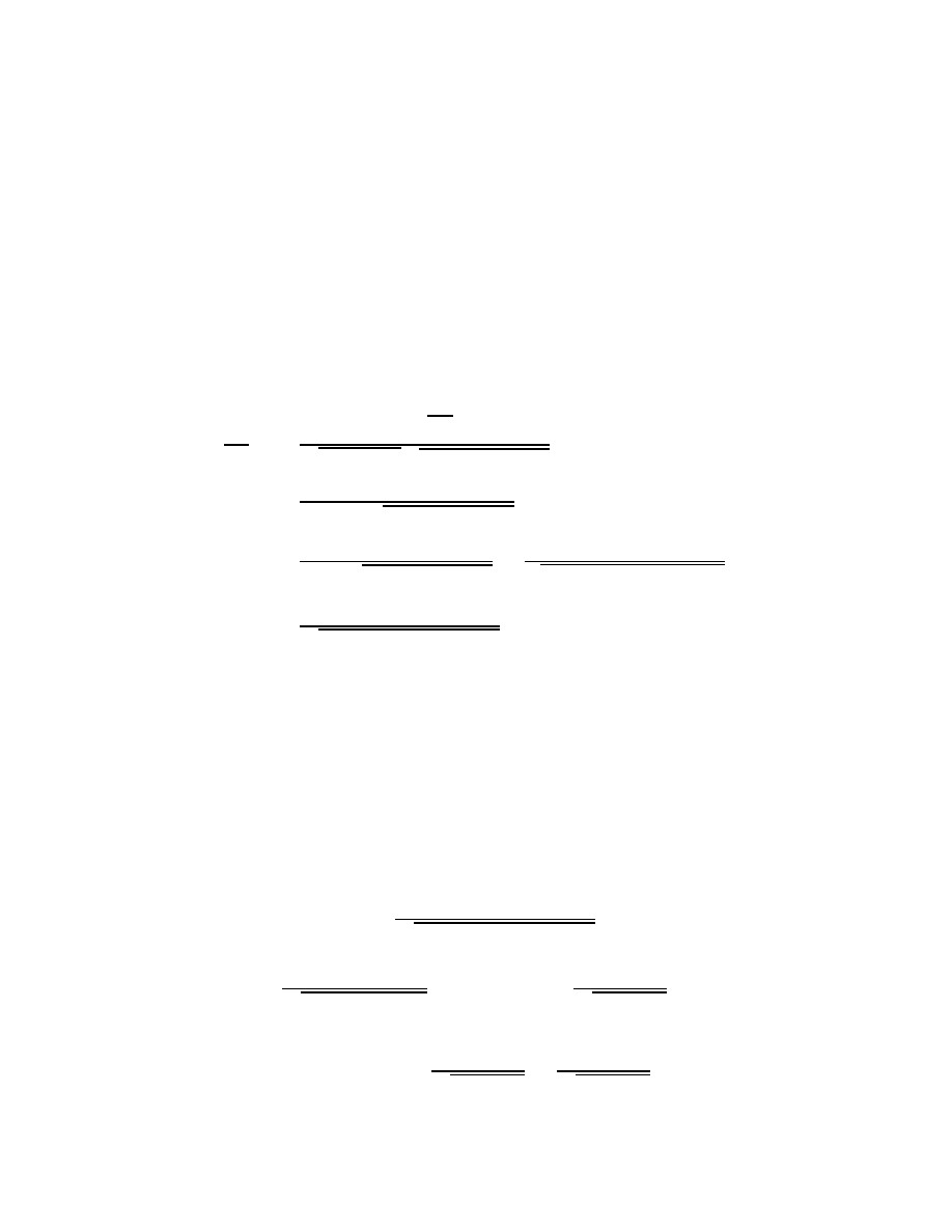
Solution. First,
X
1
= (−R sin u cos v, R cos u cos v, 0)
X
2
= (−R cos u sin v, −R sin u sin v, R cos v)
E = g
11
=
X
1
·
X
1
= R
2
cos
2
v
G = g
22
=
X
2
·
X
2
= R
2
sin
2
v + R
2
cos
2
v = R
2
.
Then
du
dv
=
h
√
R
2
√
R
2
cos
2
v
√
R
2
cos
2
v − h
2
=
hR
R cos v
√
R
2
cos
2
v − h
2
since v ∈ (−π/2, π/2)
=
h sec v
cos v
√
R
2
− h
2
sec
2
v
=
h sec
2
R
2
− h
2
(1 + tan
2
v)
=
h sec
2
v
√
R
2
− h
2
− h
2
tan
2
v
.
Example (Exercise 1.7.14(b)). Substitute w = h tan v and integrate
the above equation to obtain cos(u − u
0
) + γ tan v = 0 where u
0
and γ
are constants.
Solution. With w = h tan v, dw = h sec
2
v dv and so
u =
h
2
sec
2
v
√
R
2
− h
2
− h
2
tan
2
v
dv
= −
−1
√
R
2
− h
2
− w
2
dw = − cos
−1
w
√
R
2
− h
2
+ u
0
.
Therefore
cos(u − u
0
) =
w
√
R
2
− h
2
=
h tan v
√
R
2
− h
2
.
16

With γ = −h/
√
R
2
− h
2
we have
cos(u − u
0
) + γ tan v = 0.
17
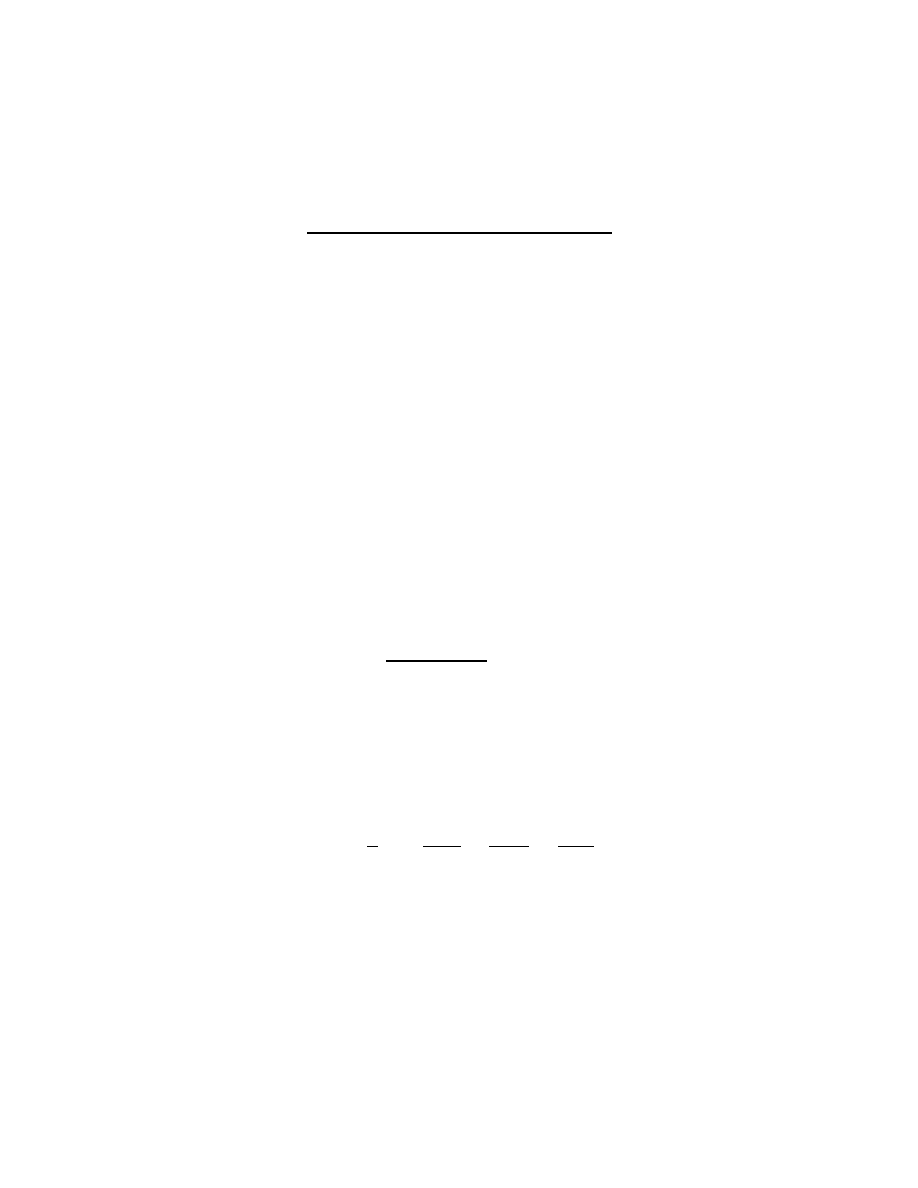
1.8 The Curvature Tensor and the
Theorema Egregium
Recall. A property of a surface which depends only on the metric
form is an intrinsic property. We have shown (Theorem I-5) that the
Gauss curvature at a point
P is K( P) = L/g where L is the Second
Fundamental Form and g is the determinate of the matrix of the First
Fundamental Form (or metric form). Therefore, to show that curvature
is an intrinsic property of a surface, we need to show that L is a function
of the g
ij
(and their derivatives) which make up the metric form.
Recall. For a surface M determined by
X(u
1
, u
2
) the coefficients of
the Second Fundamental Form are
L
ij
=
X
ij
· U =
X
ij
·
X
1
×
X
2
X
1
×
X
2
(equation (20), page 44)
and
L
i
j
= L
jk
g
ki
(equation (27), page 54)
and the Christoffel symbols are
Γ
r
ij
=
1
2
g
kr
∂g
ik
∂u
j
+
∂g
jk
∂u
i
−
∂g
ij
∂u
k
(equation (37), page 60). Also recall the formulas of Gauss
X
jk
= Γ
h
jk
X
h
+ L
jk
U (equation (17), page 43)
and the formulas of Weingarten
U
i
= −L
j
i
X
j
(equation (28), page 55).
1
Lemma. The coefficients of the Second Fundamental Form and the
Christoffel symbols are related as follows (for h = 1, 2):
∂Γ
h
ik
∂u
j
−
∂Γ
h
ij
∂u
k
+ Γ
r
ik
Γ
h
rj
− Γ
r
ij
Γ
h
rk
= L
ik
L
h
j
− L
ij
L
h
k
.
Proof. Differentiating the formulas of Gauss:
∂
X
ik
∂u
j
=
∂Γ
h
ik
∂u
j
X
h
+ Γ
h
ik
∂
X
h
∂u
j
+
∂L
ik
∂u
j
U + L
ik
∂ U
∂u
j
or by defining ∂/∂u
j
with a subscript of j
X
ikj
=
∂Γ
h
ik
∂u
j
X
h
+ Γ
h
ik
X
hj
+
∂L
ik
∂u
j
U + L
ik
U
j
.
Using the formulas of Gauss and Weingarten to rewrite
X
hj
and
U
j
we
get
X
ikj
=
∂Γ
h
ik
∂u
j
X
h
+ Γ
h
ik
(Γ
r
hj
X
r
+ L
hj
U) + ∂L
ik
∂u
j
U + L
ik
(−L
h
j
X
h
)
or (by interchanging h and r in the second term [since we are summing
over both])
X
ikj
=
∂Γ
h
ik
∂u
j
X
h
+ Γ
r
ik
(Γ
h
rj
X
h
+ L
rj
U) + ∂L
ik
∂u
j
U + L
ik
(−L
h
j
X
h
)
=
∂Γ
h
ik
∂u
j
+ Γ
r
ik
Γ
h
rj
− L
ik
L
h
j
X
h
+
Γ
r
ik
L
rj
+
∂L
ik
∂u
j
U. (49)
Interchanging j and k gives
X
ijk
=
∂Γ
h
ij
∂u
k
+ Γ
r
ij
Γ
h
rk
− L
ij
L
h
k
X
h
+
Γ
r
ij
L
rk
+
∂L
ij
∂u
k
U (50)
(so we have
X
ijk
broken into a component normal to surface M and
components which lie in the tangent plane to M at a given point -
2
namely the components in directions
X
1
and
X
2
). We have assumed
that
X is sufficiently continuous that
X
ikj
=
X
ijk
and so
X
ikj
−
X
ijk
= 0.
Subtracting (50) from (49) and using the fact that the coefficients of
X
1
and
X
2
in the resultant are 0 we have
∂Γ
h
ik
∂u
j
−
∂Γ
h
ij
∂u
k
+ Γ
r
ik
Γ
h
rj
− Γ
r
ij
Γ
h
rk
− L
ik
L
h
j
+ L
ij
L
h
k
= 0
for h = 1, 2 and the result follows.
Definition. For a surface M with Christoffel symbols as above, define
R
h
ijk
=
∂Γ
h
ik
∂u
j
−
∂Γ
h
ij
∂u
k
+ Γ
r
ik
Γ
h
rj
− Γ
r
ij
Γ
h
rk
.
These make up the Riemann-Christoffel curvature tensor (with h =
1, 2).
Note. Since the Christoffel symbols (Γ
k
ij
’s) are intrinsic properties of
surface M, the Riemann-Christoffel curvature tensor is also an intrinsic
property of M.
Note. Interchanging j and k we trivially have R
h
ijk
= −R
h
ikj
.
Theorem I-11. Gauss’ Theorema Egregium.
The Gauss curvature of a surface is an intrinsic property. That is,
the Gauss curvature of a surface is a function of the coefficients of the
metric form and their derivatives.
Proof. From the lemma and definition of R
h
ijk
we have
R
h
ijk
= L
ik
L
h
j
− L
ij
L
h
k
.
(54)
3
Now define R
mijk
= g
mh
R
h
ijk
= g
mr
R
r
ijk
. Then R
r
ijk
= g
mr
R
mijk
. Now the
Riemann-Christoffel curvature symbols R
h
ijk
are intrinsic and therefore
R
mijk
are also intrinsic. Multiplying (54) by g
mh
gives (summing over
h = 1, 2)
g
mh
R
h
ijk
= g
mh
L
ik
L
h
j
− g
mh
L
ij
L
h
k
= g
hm
L
ik
L
h
j
− g
hm
L
ij
L
h
k
or R
mijk
= L
ik
L
jm
− L
ij
L
km
since g
im
L
i
j
= L
jm
(page 54, line after
equation (27)). In particular, with m, j = 1 and i, k = 2
R
1212
= L
22
L
11
− L
21
L
21
= L
11
L
22
− L
12
L
21
(since L
ij
= L
ji
- see equation (20), page 44)
= det(L
ij
) = L.
Therefore, since R
mijk
are intrinsic, then L is intrinsic and K = L/g =
R
1212
/g is intrinsic!
Note. We now give an explicit equation for K in terms of the metric
form.
Corollary. For a surface M determined by
X(u, v) =
X(u
1
, u
2
) the
curvature is given by
K =
1
g
F
uv
−
1
2
E
vv
−
1
2
G
uu
+ (Γ
h
12
Γ
r
12
− Γ
h
22
Γ
r
11
)g
rh
where
g
11
=
X
1
·
X
1
= E
g
12
=
X
1
·
X
2
= F = g
21
4
g
22
=
X
2
·
X
2
= G
g = det(g
ij
)
and
Γ
r
ij
=
1
2
g
kr
∂g
ik
∂u
j
+
∂g
jk
∂u
i
−
∂g
ij
∂u
k
where (g
ij
)
−1
= (g
ij
).
Proof. Since R
mijk
= g
mh
R
h
ijk
(equation (55), page 76) and
R
h
ijk
=
∂Γ
h
ik
∂u
j
−
∂Γ
h
ij
∂u
k
+ Γ
r
ik
Γ
h
rj
− Γ
r
ij
Γ
h
rk
(equation (52), page 75) then
g
mh
R
h
ijk
= g
mh
∂Γ
h
ik
∂u
j
+ g
mh
Γ
r
ik
Γ
h
rj
− g
mh
∂Γ
h
ij
∂u
k
− g
mh
Γ
r
ij
Γ
h
rk
or
R
mijk
= g
mh
∂Γ
h
ik
∂u
j
+ g
hm
Γ
h
rj
Γ
r
ik
− g
mh
∂Γ
h
ij
∂u
k
− g
hm
Γ
h
rk
Γ
r
ij
(since g
hm
= g
mh
)
= g
mh
∂Γ
h
ik
∂u
j
+ Γ
rjm
Γ
r
ik
− g
mh
∂Γ
h
ij
∂u
k
− Γ
rkm
Γ
r
ij
(∗)
since Γ
ijk
= Γ
r
ij
g
rk
(equation (33), page 59). Now, interchanging the
indices in equation (33) we have g
mh
Γ
h
ik
= Γ
ikm
or differentiating with
respect to u
j
∂g
mk
∂u
j
Γ
h
ik
+ g
mh
∂Γ
h
ik
∂u
j
=
∂Γ
ikm
∂u
j
or
g
mh
∂Γ
h
ik
∂u
j
=
∂Γ
ikm
∂u
j
− Γ
h
ik
∂g
hm
∂u
j
.
(∗∗)
Now using (∗∗) in (∗) we have
R
mijk
=
∂Γ
ikm
∂u
j
− Γ
h
ik
∂g
hm
∂u
j
+ Γ
rjm
Γ
r
ik
−
∂Γ
ijm
∂u
k
− Γ
h
ij
∂g
hm
∂u
k
−Γ
rkm
Γ
r
ij
.
5

Replacing r by h in the products of Γ’s gives
R
mijk
=
∂Γ
ikm
∂u
j
− Γ
h
ik
∂g
hm
∂u
j
+Γ
hjm
Γ
h
ik
−
∂Γ
ijm
∂u
k
− Γ
h
ij
∂g
hm
∂u
k
−Γ
hkm
Γ
h
ij
.
Now
Γ
ikm
=
1
2
∂g
im
∂u
k
+
∂g
mk
∂u
i
−
∂g
ki
∂u
m
(equation (36), page 60)
and
∂g
hm
∂u
j
= Γ
hjm
+ Γ
mjh
(equation (35), page 60)
= Γ
hjm
+ Γ
r
mj
g
rh
(equation (33), page 59)
so
R
mijk
=
∂
∂u
j
1
2
∂g
im
∂u
k
+
∂g
mk
∂u
i
−
∂g
ki
∂u
m
+Γ
h
ik
Γ
hjm
− Γ
h
ik
(Γ
hjm
+ Γ
r
mj
g
rh
)
−
∂
∂u
k
1
2
∂g
im
∂u
j
+
∂g
mj
∂u
i
−
∂g
ji
∂u
m
−Γ
h
ij
Γ
hkm
+ Γ
h
ij
(Γ
hkm
+ Γ
r
mk
g
rh
)
=
1
2
∂
2
g
im
∂u
j
∂u
k
+
∂
2
g
mk
∂u
j
∂u
i
−
∂
2
g
ki
∂u
j
∂u
m
+Γ
h
ik
Γ
hjm
− Γ
h
ik
(Γ
hjm
+ Γ
r
mj
g
rh
)
−
1
2
∂
2
g
im
∂u
k
∂u
j
+
∂
2
g
mj
∂u
k
∂u
i
−
∂
2
g
ji
∂u
k
∂u
m
−Γ
h
ij
Γ
hkm
+ Γ
h
ij
(Γ
hkm
+ Γ
r
mk
g
rh
)
=
1
2
∂
2
g
km
∂u
j
∂u
i
−
∂
2
g
jm
∂u
i
∂u
k
+
∂
2
g
ij
∂u
k
∂u
m
−
∂
2
g
ik
∂u
j
∂u
m
+(Γ
h
ij
Γ
r
mk
− Γ
h
ik
Γ
r
mj
)g
rh
.
So with m = j = 1 and i = k = 2
R
1212
=
1
2
∂
2
g
21
∂u
1
∂u
2
−
∂
2
g
11
∂u
2
∂u
2
+
∂
2
g
21
∂u
2
∂u
1
−
∂
2
g
22
∂u
1
∂u
1
6

+(Γ
h
21
Γ
r
12
− Γ
h
22
Γ
r
11
)g
rh
=
1
2
(F
uv
− E
vv
+ F
uv
− G
uu
) + (Γ
h
21
Γ
r
12
− Γ
h
22
Γ
r
11
)g
rh
.
Since K = R
1212
/g (equation (57), page 76), and the result follows.
Corollary. For a surface M determined by
X(u, v) with orthogonal
coordinates (
X
1
·
X
2
= F = 0) the curvature is
K =
1
2
√
EG
∂
∂u
G
u
√
EG
+
∂
∂v
E
v
√
EG
.
Proof. With F = 0 and equation (40) of page 62 (which gives the
Christoffel symbols in an orthogonal coordinate system in terms of E
and G) we have
K =
1
EG
−
1
2
E
vv
−
1
2
G
uu
+ ((Γ
1
12
)
2
− Γ
1
22
Γ
1
11
)g
11
+ ((Γ
2
12
)
2
− Γ
2
22
Γ
2
11
)g
22
(since g
12
= g
21
= 0 and det(g
ij
) = g
11
g
22
= EG)
=
1
EG
−
1
2
E
vv
−
1
2
G
uu
+
E
v
2E
2
−
−
G
u
2E
E
u
2E
E
+
G
u
2G
2
−
G
v
2G
−
E
v
2G
G
=
1
EG
−
1
2
E
vv
−
1
2
G
uu
+
E
2
v
4E
2
+
E
u
G
u
4E
2
E +
G
2
u
4G
2
+
E
v
G
v
4G
2
G
= −
1
EG
1
2
E
vv
+
1
2
G
uu
−
EE
2
v
+ EE
u
G
u
4E
2
−
GG
2
u
+ E
v
GG
v
4G
2
=
−1
2EG
√
EG
√
EGE
vv
+
√
EGG
uu
−
√
EG
E
2
v
+ E
u
G
u
2E
−
√
EG
G
2
u
+ E
v
G
v
2G
=
−1
2EG
√
EG
√
EGE
vv
+
√
EGG
uu
−
GE
2
v
+ E
u
GG
u
2
√
EG
7
−
EG
2
u
+ EE
v
G
v
2
√
EG
=
−1
2EG
√
EG
√
EGE
vv
+
√
EGG
uu
−
G
u
(EG
u
+ E
u
G)
2
√
EG
−
E
v
(EG
v
+ E
v
G)
2
√
EG
=
−1
2
√
EG
√
EGG
uu
−
G
u
(EG
u
+E
u
G)
2
√
EG
EG
+
√
EGE
vv
−
E
v
(EG
v
+E
v
G)
2
√
EG
EG
=
−1
2
√
EG
∂
∂u
G
u
√
EG
+
∂
∂v
E
v
√
EG
.
Note. The equation given in the previous corollary will be useful in
the exercises in this section.
Note. Some symmetry relations in R
mijk
are given at the end of the
section.
Example (Exercise 2, page 80). Let
X(u, v) = (f(u) cos v, f(u) sin v, g(u))
be a surface of revolution whose profile curve α(u) = (f (u), 0, g(u)) has
unit speed. Show that K = −f
/f.
Solution. By Exercise 1.4.5, page 39, E = g
11
= (f
(u))
2
+ (g
(u))
2
,
F = g
12
= g
21
= 0 (coordinates are orthogonal), G = g
22
= (f (u))
2
. So
8

by equation (59), page 78,
K =
−1
2
(f (u))
2
{(f
(u))
2
+ (g
(u))
2
}
×
∂
∂u
2f (u)f
(u)
(f (u))
2
{(f
(u))
2
+ (g
(u))
2
}
+
∂
∂v
[0]
.
Now assuming α
=
(f
(u))
2
+ (g
(u))
2
= 1 and f (u) ≥ 0:
K =
−1
2f (u)
∂
∂u
[2f
(u)]
=
−f
(u)
f(u)
.
Example (Exercise 5 (b), page 81). The pseudosphere may be
represented as the surface of revolution
X(u, v) =
a sin u cos v, a sin u sin v, a
cos u + ln
tan
u
2
for u ∈ (0, π/2). Show that K = −1/a
2
(and so the pseudosphere has
constant negative curvature).
Solution. In Exercise 5 (a), you will show that E = a
2
cot
2
u and
G = a
2
sin
2
u. Therefore by equation (59), page 78:
K =
−1
2
√
a
4
cot
2
u sin
2
u
∂
∂u
2a
2
sin u cos u
√
a
4
cot
2
u sin
2
u
+
∂
∂v
[0]
=
−1
2a
4
cot
2
u sin
2
u
∂
∂u
2a
2
sin u cos u
a
4
cot
2
u sin
2
u
since u ∈ (0, π/2)
=
−1
2a
4
cot
2
u sin
2
u
∂
∂u
[2 sin u]
=
−1
2a
4
cot
2
u sin
2
u
(2 cos u) =
− cot u
a
2
cot u
=
−1
a
2
.
9
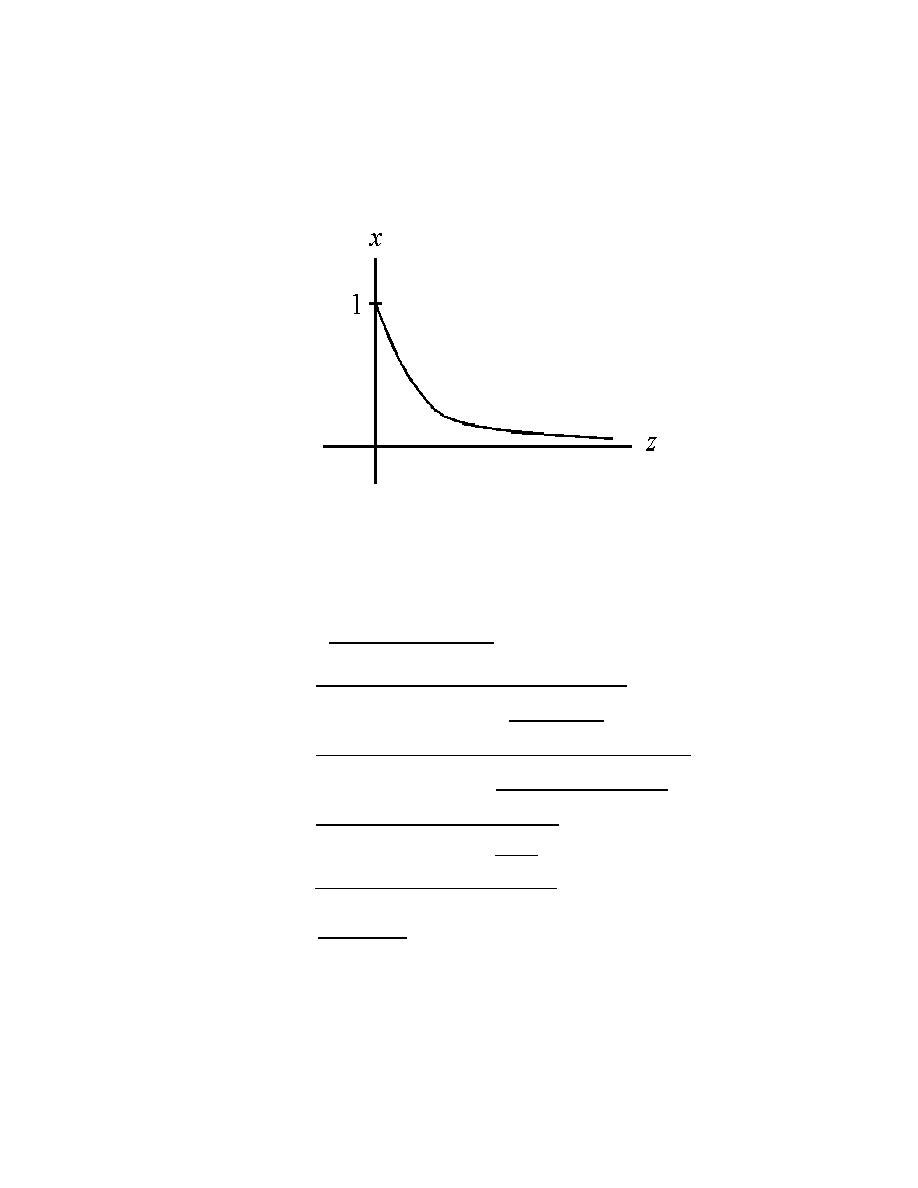
Note. In the zx−plane, the profile curve of the pseudosphere is
We get the point (z, x) = (0, 1) for u = π/2. Let’s calculate the ar-
clength s for u ranging from π/2 to u
∗
:
s = −
u
∗
π/2
(x
(u))
2
+ (z
(u))
2
du (since u
∗
< π/2)
=
π/2
u
∗
cos
2
(u) +
− sin u +
sec
2
(u/2)
2 tan(u/2)
2
du
=
π/2
u
∗
cos
2
u +
− sin u +
1
2 sin(u/2) cos(u/2)
2
du
=
π/2
u
∗
cos
2
u +
− sin u +
1
sin u
2
du
=
π/2
u
∗
cos
2
u + sin
2
u − 2 + csc
2
u d u
=
π/2
u
∗
√
csc
2
u − 1 du =
π/2
u
∗
| cot u| du
=
π/2
u
∗
cot u d u = ln(sin u)
π/2
u
∗
= − ln(sin u
∗
).
10
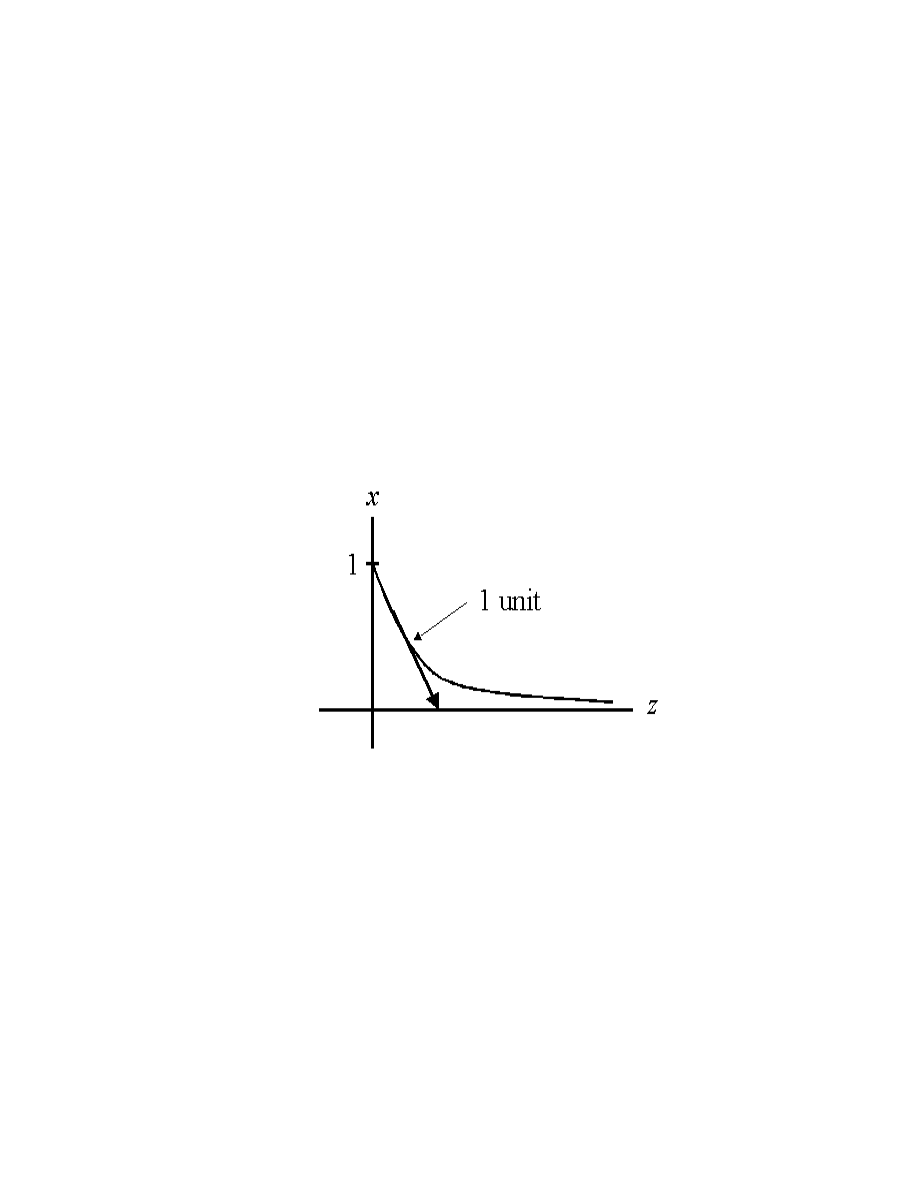
Therefore
exp(−arclength) = e
−s
= e
−(− ln(sin u
∗
))
= sin u
∗
= x
∗
.
So we have x = e
−s
where s is arclength. This curve is called a tractrix.
It can be generated by placing a box at point (0, 1) and dragging it
by attaching a 1 unit rope and pulling along the z−axis (therefore the
tangent line at any point meets the z−axis 1 unit from the point of
tangency):
11

1.9 Manifolds
Note. In this section, we extend the ideas of tangents, metrics, geo-
desics, and curvature to “manifolds” (in a sense, “n−dimensional sur-
faces”) without appealling to how they are imbedded in a higher di-
mensional space.
Definition. Let M be a non-empty set whose elements we call points.
A coordinate patch on M is a one-to-one function
X : D → M (contin-
uous and regular) from an open subset D of E
2
(or more generally E
n
)
into M.
Note. In the following definition, by “domain” of a function we mean
the largest set on which the function is defined. By “smooth” we mean
sufficiently differentiable for our purposes. Afunction whose domain is
empty is considered smooth.
Definition I-12. An abstract surface or 2−manifold (more generally,
n−manifold) is a set M with a collection C of coordinate patches on M
satisfying:
(a) M is the union of images of the patches in C (that is, if C = {
X
i
}
and
X
i
is defined on set D
i
, then M =
i
X
i
(D
i
)).
(b) The patches of C overlap smoothly, that is if
X
1
: D
1
→ M and
X
2
:
D
2
→ M are two patches in C, then (
X
1
)
−1
◦
X
2
and (
X
2
)
−1
◦
X
1
have open domains and are smooth.
1

(c) Given two points
P
1
and
P
2
of M, there exist coordinate patches
X
1
: D
1
→ M and
X
2
: D
2
→ M in C such that P
1
∈
X
1
(D
1
),
P
2
∈
X
2
(D
2
) and
X
1
(D
1
) ∩
X
2
(D
2
) = ∅ (this is the Hausdorff
property).
(d) The collection C is maximal. That is, any coordinate patch on
M which overlaps smoothly with every patch of C is itself in C.
(Notice that two disjoint coordinate patches “overlap smoothly”
by convention).
Definition. The collection C is called a differentiable structure on M
and patches in C are called admissible patches.
Note. If properties (a), (b), and (c) of Definition I-12 are satisfied by a
collection C
then we can adjoin to C
all patches that overlap smoothly
with the patches of C
to create a collection C which satisfies (a), (b),
(c), (d). In this case, C
is said to generate C.
Example (Exercise 1.9.1). Let M be the plane with Cartesian coor-
dinates. The identity mapping of M onto itself is a coordinate patch. A
differentiable structure on M is obtained by adjoining to this mapping
all patches in M which overlap smoothly with this mapping. The polar
coordinate patch
u = r cos θ
v = r sin θ
(r, θ) ∈ D
overlaps smoothly with the identity patch IF D is of the form
2
D = {(r, θ) | r > 0, θ ∈ (a, b), b − a ≤ 2π}
(an open sector).
Solution. Let
X : D → M and X : D → M. By definition,
X and
X overlap smoothly if ( X)
−1
◦ X (which maps D → M → D) and
(
X)
−1
◦
X (which maps D → M → D) have open domains and are
smooth.
First,
X and X are one-to-one and so are invertible. Explicitly,
(
X)
−1
◦ X(r, θ) = (x, y) = (r cos θ, r sin θ).
So
∂
∂r
[(
X)
−1
◦ X] = (cos θ, sin θ)
and
∂
∂θ
[(
X)
−1
◦ X] = (−r sin θ, r cos θ).
Therefore, (
X)
−1
◦ X is smooth (the first partials are continuous... in
fact, it is infinitely differentiable). Similarly, (
X)
−1
◦
X(x, y) = (r, θ)
where r =
√
x
2
+ y
2
and tan θ = y/x where we choose θ such that
θ ∈ (a, b),
θ is in Quadrant I if x > 0, y > 0,
θ is in Quadrant II if x < 0, y > 0,
θ is in Quadrant III if x < 0, y < 0,
θ is in Quadrant IV if x > 0, y < 0,
(and similar choices are made if x = 0 or y = 0). So θ = tan
−1
(y/x) +
constant
θ
(so θ is a continuous function of (x, y), even though tan
−1
(y/x)
3

is not continuous — this is how we choose the θ to associate with (x, y)).
We then have
∂
∂x
[(
X
−1
◦
X)] =
x
√
x
2
+ y
2
,
−y/x
2
1 + (y/x)
2
and
∂
∂y
[(
X
−1
◦
X)] =
y
√
x
2
+ y
2
,
1/x
1 + (y/x)
2
,
therefore (since (x, y) = (0, 0)) (
X)
−1
◦
X is smooth (in fact, infinitely
differentiable). Next, the domain of (
X)
−1
◦
X : D → D is D itself and
D is open (by definition). The domain of (
X)
−1
◦ X : D → D is the set
of all (x, y) ∈ M such that
√
x
2
+ y
2
= r > 0 and tan
−1
(y/x) ∈ (a, b)
(where tan
−1
(y/x) is calculated as described above). Therefore the
domain of (
X)
−1
◦
X is open. Hence,
X and X overlap smoothly.
Definition. An admissible patch
X : D → M associates with each
point
P of
X(D) a unique ordered pair (or in general, ordered n−tuple)
(u
1
, u
2
) =
X
−1
(
P ) called a local coordinate of P with respect to
X.
Note. Apoint
P can have different local coordinates with respect to
different admissible patches. Suppose, for example,
P =
X(u
1
, u
2
) =
X(u
1
, u
2
). Then (
X)
−1
◦ X(u
1
, u
2
) = (u
1
, u
2
) and (
X)
−1
◦
X
1
(u
1
, u
2
) =
(u
1
, u
2
).
Definition. In the above setting, the equations (
X)
−1
◦ X(u
1
, u
2
) =
(u
1
, u
2
) and (
X)
−1
◦
X(u
1
, u
1
) = (u
1
, u
2
) are changes of coordinates. See
Figure I-29, page 83. In terms of local coordinates:
X
−1
◦
X is given by u
i
= u
i
(u
1
, u
2
), i = 1, 2
(61a)
X
−1
◦ X is given by u
i
= u
i
(u
1
, u
2
), i = 1, 2.
(61b)
4
Definition I-13. Aset Ω ⊂ M is a neighborhood of a point
P ∈ M if
there exists an admissible patch
X : D → M such that P ∈
X(D) and
X(D) ⊂ Ω. Asubset of M is open if it is a neighborhood of each of its
points.
Definition. Let Ω be an open subset of the 2-manifold (or generally
n−manifold) M. Afunction f : Ω → R is smooth if f ◦
X is smooth
for every admissible patch
X in M (notice f ◦
X maps E
2
[or more
generally E
n
] to Ω and then to R - so the idea of differentiability is
clearly defined). For f : Ω → R smooth and
X : D → M an admissible
patch whose image intersects Ω, define
∂f
∂u
i
:
X(D) ∩ Ω → R for i = 1, 2 (or generally i = 1, 2, . . . , n)
as
∂f
∂u
i
=
∂(f ◦
X)
∂u
i
◦
X
−1
.
This is called the partial derivative of f with respect to u
i
.
Note. For
P ∈
X(D) ∩ Ω:
∂f
∂u
i
(
P ) =
∂(f ◦
X)
∂u
i
(
X
−1
(
P )).
The mappings are:
X
−1
∂(f ◦
X)
∂u
i
P ∈ M −→ (u
1
, u
2
)
−→ R.
The usual product rules hold:
∂
∂u
i
(fg) =
∂f
∂u
i
g + f
∂g
∂u
i
5
where f and g have common domain.
Definition. For
P ∈
X(D), define an operator on the collection of
functions smooth in a neighborhood of
P as
∂
∂u
i
(
P )[f] =
∂f
∂u
i
(
P ).
Notation. Asuperscript which appears in the denominator, such as
∂/∂u
i
, counts as a subscript and therefore will impact the Einstein
summation notation. (The motivation is that partial differentiation is
usually denoted with subscripts.)
Note. If
X : D → M and X : D → M are admissible patches, then
on the overlap
X(D) ∩ X(D) we have from equation (61), page 83, the
operator identities
∂
∂u
i
=
∂u
j
∂u
i
∂
∂u
j
for i = 1, 2
(63a)
∂
∂u
k
=
∂u
i
∂u
k
∂
∂u
i
for k = 1, 2
(63b)
Definition I-14. Let m ∈ Z
+
and suppose O is an open subset of E
m
.
Afunction f : O → M is smooth if
X
−1
◦ f (which maps E
m
to E
n
) is
smooth for every admissible patch
X on M. If O is not open, we say
f : O → M is smooth if f is smooth on an open set containing O. A
curve in M is a smooth function from an interval (a connected subset
of R) into M.
6
Note. Now for tangent vectors and planes. We replace the idea of
vectors as arrows, with the idea of vectors as operators. Remember
that a vector is something which satisfies the properties given in the
definition of a vector space! The “arrows” idea is just (technically) an
aid in visualization!
Definition I-15. Let α : I → M be a curve on a 2-manifold (or
generally, n−manifold) M. For t ∈ I, define the velocity vector of α at
α(t) as the operator
α
(t)[f ] = (f ◦ α)
(t) =
d
dt
[f (α(t))]
for each smooth f which maps an open neighborhood of α(t) into R.
Definition I-16. Let
P be a point of the 2−manifold M. An operator
v which assigns a real number v[f] to each smooth real-valued function
f on M is called a tangent vector to M at P if there exists a curve in M
which passes through
P and has velocity v at P. The set of all tangent
vectors to M at
P is called the tangent plane of M at P, denoted T
P
M.
Note. The previous two definitions are independent of the choice of
coordinate patch (although we may do computations in some coordinate
patch).
Theorem. Let
P be a point on manifold M and let
X be an admissible
coordinate patch such that
P =
X(u
1
(t
0
), u
2
(t
0
)). If v is a tangent
vector to M at
P then v is a linear combination of
∂
∂u
1
(
P ) and
∂
∂u
2
(
P ).
7

Proof. With v a tangent vector, there is a curve α(t) in M such that
α(t
0
) =
P and α
(t
0
) = v. Let f be a smooth real-valued function.
Then with α(t) =
X(u
1
(t), u
2
(t)),
v(t)[f] = α
(t)[f ] =
d
dt
[(f ◦ α)(t)]
=
d
dt
[f ◦
X(u
1
(t), u
2
(t))] =
∂(f ◦
X)
∂u
i
(u
1
(t), u
2
(t))
du
i
dt
=
∂(f ◦
X)
∂u
i
(
X
−1
◦ α(t))
du
i
dt
=
∂f
∂u
i
(α(t))u
i
(t) (by definition)
= u
i
(t)
∂f
∂u
i
(α(t)).
So as an operator, α
(t) = u
i
(t)
∂
∂u
i
(α(t)), or simply
α
= u
i
∂
∂u
i
.
(64)
A t point
P ,
v = α
(t
0
) = u
i
(t
0
)
∂
∂u
i
(
P ) = v
i
∂
∂u
i
(
P )
where v
i
= u
i
(t
0
).
Note. The vector
∂
∂u
1
(
P ) and
∂
∂u
2
(
P ) are linearly independent (con-
sider their behavior on functions of the form f (u
1
, u
2
) = u
1
and g(u
1
, u
2
) =
u
2
... although this argument is weak!). So the vectors form a basis for
a 2-dimensional vector space, the tangent plane to M at
P , T
P
M. In
general, a tangent plane to an n−manifold is an n−dimensional vector
space (a “hyperplane”).
Note. The converse of the Theorem also holds: If v is a linear com-
bination of
∂
∂u
1
(
P ) and
∂
∂u
2
(
P ), then v is a tangent vector to M at
P.
8
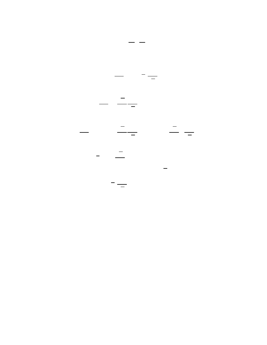
Note. Suppose
X : D → M and X : D → M are overlapping admissi-
ble patches at
P . Then tangent vector v has two coordinate represen-
tations:
v = v
i
∂
∂u
i
(
P ) = v
j
∂
∂u
j
(
P ).
From equation (63a), page 85, we have
∂
∂u
i
=
∂u
j
∂u
i
∂
∂u
j
for i = 1, 2
and so
v = v
i
∂
∂u
i
(
P ) = v
i
∂u
j
∂u
i
∂
∂u
j
(
P ) =
v
i
∂u
j
∂u
i
∂
∂u
j
(
P )
and so
v
j
= v
i
∂u
j
∂u
i
for j = 1, 2
(67a)
(remember the linear independence of the ∂/∂
u
j
’s). Similarly
v
i
= v
j
∂
∂u
j
(
P ) for i = 1, 2.
This gives us a relationship between the coordinates of tangent vectors.
Notice that all these ideas extend to higher dimensions.
Note. We now introduce an inner product which generalizes the idea of
a dot product and use this to carry over several of the ideas developed
earlier for surfaces to manifolds.
Definition I-17. Let V be a vector space with scalar field R. A n
inner product on V is a mapping ·, · : V × V → R such that for all
v,v
, w, w
∈ V and for all a, a
∈ R:
(a) v,
w = w,v (symmetry).
9
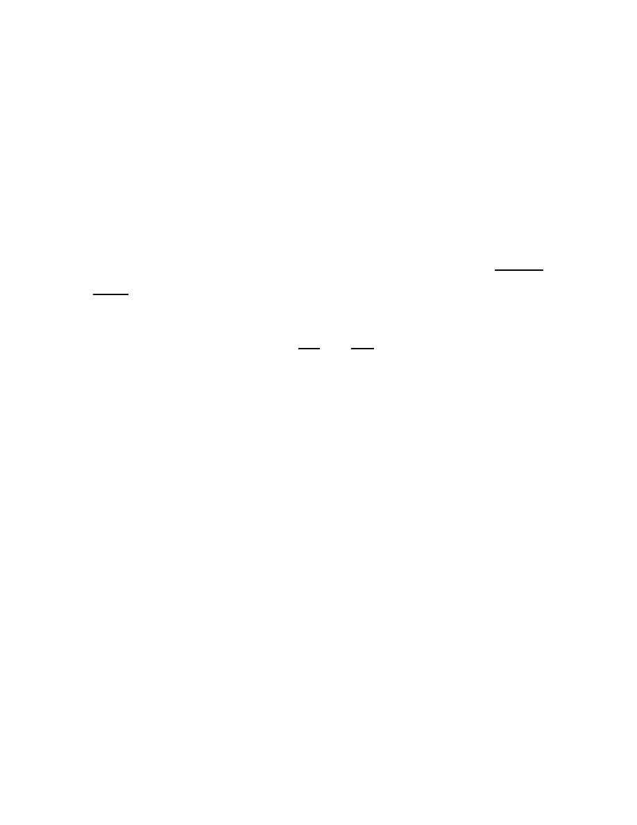
(b) av + a
v
, w = av, w + a
v
, w and v, aw + a
w
= av, w +
a
v, w
(bilinear).
(c) v, v ≥ 0 for all v ∈ V and v, v = 0 if and only if v = 0 (positive
definite).
Definition I-18. A Riemannian metric (or simply metric) on an
2−manifold M is an assignment of an inner product to each tangent
plane of M. For each coordinate patch
X : D → M, we require the
functions g
ij
:
X(D) → R defined as
g
ij
(
P ) =
∂
∂u
i
(
P ),
∂
∂u
j
(
P )
for i, j = 1, 2, . . . , n to be smooth. An n−manifold with such a Rie-
mannian metric is called a Riemannian n−manifold.
Example. R
n
is a Riemannian manifold where the tangent planes are
themselves R
n
(since R
n
is “flat”) and the inner product is the usual
dot product in R
n
.
Example. All the surfaces we dealt with earlier are examples of Rie-
mannian 2-manifolds (well... technically, a manifold does not have a
boundary, so we might have to throw out some of the examples [such as
the pseudosphere], although we could include in a study the so called
“manifolds with a boundary”).
Definition. Avector space V with a mapping ·, · : V × V → R
satisfying (a) and (b) given above along with
10
(c
) If v,
w = 0 for all w ∈ V, then v = 0 (nonsingular).
is a semi-Riemannian n−manifold (again, we require g
ij
(
P ) to be smooth).
Note. Condition (c
) is weaker than condition (c) (and so every Rie-
mannian n−manifold is also a semi-Riemannian n−manifold). Con-
dition (c
) allows lengths of vectors to be negative. We will see that
spacetime is a semi-Riemannian 4-manifold.
Note. If
X : D → M and X : D → M are overlapping admissible
patches then
g
mn
= g
ij
∂u
i
∂u
m
∂u
j
∂u
n
for m, n = 1, 2,
g
ij
= g
mn
∂u
m
∂u
i
∂u
n
∂u
j
for i, j = 1, 2.
(You will verify these as homework.)
Theorem. If v and
w are tangent vectors at P to a semi-Riemannian
n−manifold M, and if
X : D → M, X : D → M are admissible patches
with
P ∈
X(D) ∩ X(D) then
g
ij
v
i
w
j
= g
ij
v
i
w
j
.
Therefore g
ij
v
i
w
j
is called an invariant.
Proof. We have v = v
i
∂
∂u
i
and
w = w
j
∂
∂u
j
, so
v, w =
v
i
∂
∂u
i
, w
j
∂
∂u
j
= v
i
∂
∂u
i
, w
j
∂
∂u
j
= v
i
w
j
∂
∂u
i
,
∂
∂u
j
= g
ij
v
i
w
j
.
11
Similarly, with v = v
i
∂
∂u
i
and
w = w
j
∂
∂u
j
we have v,
w = g
ij
v
i
w
j
.
Therefore g
ij
v
i
w
j
= g
ij
v
i
w
j
. (This is consistent with the fact that inner
products are independent of the choice of coordinates).
Note. We see from the above theorem, that the g
ij
’s determine inner
products of tangent vectors to a manifold just as the g
ij
’s of Section
1.4 determined dot products of tangent vectors to a surface.
Definition. Let v be a tangent vector to a semi-Riemannian n−manifold.
Then define v = v, v
1/2
. For α(t), a ≤ t ≤ b a curve in M, define
the arclength of α as
L =
b
a
α
(t) dt.
Note. Let s(t) = s denote the arc length along the curve from α(a) to
α(t). Then
s(t) =
t
a
α
(t
∗
) dt
∗
and so s
(t) = α
(t) and
(s
(t))
2
=
ds
dt
2
= α
(t)
2
= α
(t), α
(t).
Let
X : D → M be an admissible coordinate patch defined in a neigh-
borhood of α(t). Then α
= α
i
∂
∂u
i
= u
i
∂
∂u
i
(by equation (64), page
86) and as in the above Theorem
α
(t), α
(t) =
u
i
∂
∂u
i
, u
j
∂
∂u
j
= u
i
u
j
∂
∂u
i
,
∂
∂u
j
= g
ij
u
i
u
j
= g
ij
du
i
dt
du
j
dt
.
(71)
12
Since expressions of the form g
ij
v
i
w
j
are invariant from one coordinate
system to another, arclength and expression (71) are invariant.
Definition. Let M be a semi-Riemannian manifold. The expression
ds
dt
2
= g
ij
du
i
dt
du
j
dt
(which is invariant from one “coordinate patch” to another) is the met-
ric form or the fundamental form of the manifold.
Note. We now mimic earlier sections and give a number of definitions.
Definition. Create the matrix (g
ij
) and define (g
ij
)
−1
= (g
ij
). For
each coordinate system,
X(u
1
, u
2
, . . . , u
n
) define the Christoffel symbols
of the first kind as
Γ
ijk
=
1
2
∂g
ik
∂u
j
+
∂g
jk
∂u
i
−
∂g
ij
∂u
k
and the Christoffel symbols of the second kind as
Γ
r
ij
=
1
2
g
kr
∂g
ik
∂u
j
+
∂g
jk
∂u
i
−
∂g
ij
∂u
k
.
Definition I-19. If α = α(s) is a curve in a semi-Riemannian n−manifold
M, where s is arclength, then α is a geodesic if in each local coordinate
system defined on part of α
d
2
u
r
ds
2
+ Γ
r
ij
du
i
ds
du
j
ds
= 0
for r = 1, 2, . . . , n. (compare this to equation (29), page 58.)
13

Note. Theorems I-9 and I-10 carry over to semi-Riemannian n−manifolds.
In particular, the shortest distance between two points is along a geo-
desic.
Definition. For a semi-Riemannian n−manifold, define the Riemann-
Christoffel curvature tensor as
R
h
ijk
=
∂Γ
h
ik
∂u
j
−
∂Γ
h
ij
∂u
k
+ Γ
r
ik
Γ
h
rj
− Γ
r
ij
Γ
h
rk
for h, i, j, k = 1, 2, . . . , n. Define
R
mijk
= g
mh
R
h
ijk
.
Note. The curvature tensor has n
4
entries (although there is some
symmetry). When n = 2 the only nonzero entries are
R
1212
= R
2121
= −R
2112
= −R
1221
and for 2-manifolds (as in Section 1.8), curvature is K = R
1212
/g.
However, things are much more complicated in higher dimensions!
Note. The curvature tensor R
h
ijk
for an n−manifold has n
2
(n
2
− 1)/12
independent components (so sayeth the text, page 90). Therefore
curvature for an n−manifold is NOT determined by a single number
when n > 2!
14

Example (Exercise 1.9.4). Suppose a Riemannian metric on M (an
open subset of R
2
) is given by
ds
2
=
1
γ
2
(du
2
+ dv
2
)
where γ = γ(u, v) is a smooth positive-valued function. Then M has
Gauss curvature
K = γ(γ
uu
+ γ
vv
) − (γ
2
u
+ γ
2
v
).
Proof. First, we have E = 1/γ
2
= G and F = 0. So we have from
Exercise 1.8.3
K =
−1
√
EG
∂
∂u
1
√
E
∂
√
G
∂u
+
∂
∂v
1
√
G
∂
√
E
∂v
.
Now
√
E =
√
G = 1/γ and so
K = −γγ
∂
∂u
γ
∂[1/γ]
∂u
+
∂
∂v
γ
∂[1/γ]
∂v
= −γ
2
∂
∂u
γ
−1
γ
γ
u
]
+
∂
∂v
γ
−1
γ
2
γ
v
= −γ
2
∂
∂u
−γ
u
γ
+
∂
∂v
−γ
v
γ
= −γ
2
(−γ
uu
)γ − (−γ
u
)(γ
u
)
γ
2
+
(−γ
vv
)γ − (−γ
v
)(γ
v
)
γ
2
= −γ
2
−γγ
uu
+ (γ
u
)
2
− γγ
vv
+ (γ
v
)
2
γ
2
= γ(γ
uu
+ γ
vv
) − ((γ
u
)
2
+ (γ
v
)
2
).
15
Example (Exercise 1.9.7). Let M be the subset of R
2
: M = {(u, v) |
u
2
+ v
2
< 4k
2
} (where k > 0). Introduce the metric
ds
2
=
1
γ
2
(du
2
+ dv
2
)
where γ(u, v) = 1 −
u
2
+ v
2
4k
2
. This is called the Poincare Disk. Then
K = −1/k
2
.
Proof. From Exercise 1.9.4,
K = γ(γ
uu
+ γ
vv
) − (γ
2
u
+ γ
2
v
).
Well,
γ
u
=
−u
2k
2
, γ
v
=
−v
2k
2
, γ
uu
=
−1
2k
2
, γ
vv
=
−1
2k
2
.
Therefore,
K =
1 −
u
2
+ v
2
4k
2
−1
2k
2
+
−1
2k
2
−
−u
2k
2
2
+
−v
2k
2
2
=
1 −
u
2
+ v
2
4k
2
−1
k
2
−
u
2
4k
4
2
+
v
2
4k
4
2
=
−(4k
2
− u
2
− v
2
)
4k
4
−
u
2
4k
4
−
v
2
4k
4
=
−1
k
2
.
16

Chapter 2. Special Relativity: The
Geometry of Flat Spacetime
Note. Classically (i.e in Newtonian mechanics), space is thought of as
1. unbounded and infinite,
2. 3-dimensional and explained by Euclidean geometry, and
3. “always similar and immovable” (Newton, Principia Mathematica,
1687).
This would imply that one could set up a system of spatial coordinates
(x, y, z) and describe any dynamical event in terms of these spatial
coordinates and time t.
Note. Newton’s Three Laws of Motion:
1. (The Law of Inertia) A body at rest remains at rest and a body in
motion remains in motion with a constant speed and in a straight
line, unless acted upon by an outside force.
2. The acceleration of an object is proportional to the force acting upon
it and is directed in the direction of the force. That is,
F = ma.
3. To every action there is an equal and opposite reaction.
Note. Newton also stated his Law of Universal Gravitation in Prin-
cipia:
1
“Every particle in the universe attracts every other particle
in such a way that the force between the two is directed
along the line between them and has a magnitude propor-
tional to the product of their masses and inversely propor-
tional to the square of the distance between them.” (See
page 186.)
Symbolically, F =
GMm
r
2
where F is the magnitude of the force, r the
distance between the two bodies, M and m are the masses of the bodies
involved and G is the gravitational constant (6.67 × 10
−8
cm./(g sec
2
)).
Assuming only Newton’s Law of Universal Gravitation and Newton’s
Second Law of Motion, one can derive Kepler’s Laws of Planetary Mo-
tion.
2

2.1 Inertial Frames of Reference
Definition. A frame of reference is a system of spatial coordinates and
possibly a temporal coordinate. A frame of reference in which the Law
of Inertia holds is an inertial frame or inertial system. An observer at
rest (i.e. with zero velocity) in such a system is an inertial observer.
Note. The main idea of an inertial observer in an inertial frame is that
the observer experiences no acceleration (and therefore no net force).
If S is an inertial frame and S
is a frame (i.e. coordinate system)
moving uniformly relative to S, then S
is itself an inertial frame (see
Exercise II-1). Frames S and S
are equivalent in the sense that there is
no mechanical experiment that can be conducted to determine whether
either frame is at rest or in uniform motion (that is, there is no pre-
ferred frame). This is called the Galilean (or classical) Principle of
Relativity.
Note. Special relativity deals with the observations of phenomena by
inertial observers and with the comparison of observations of inertial
observers in equivalent frames (i.e. NO ACCELERATION!). General
relativity takes into consideration the effects of acceleration (and there-
fore gravitation) on observations.
1
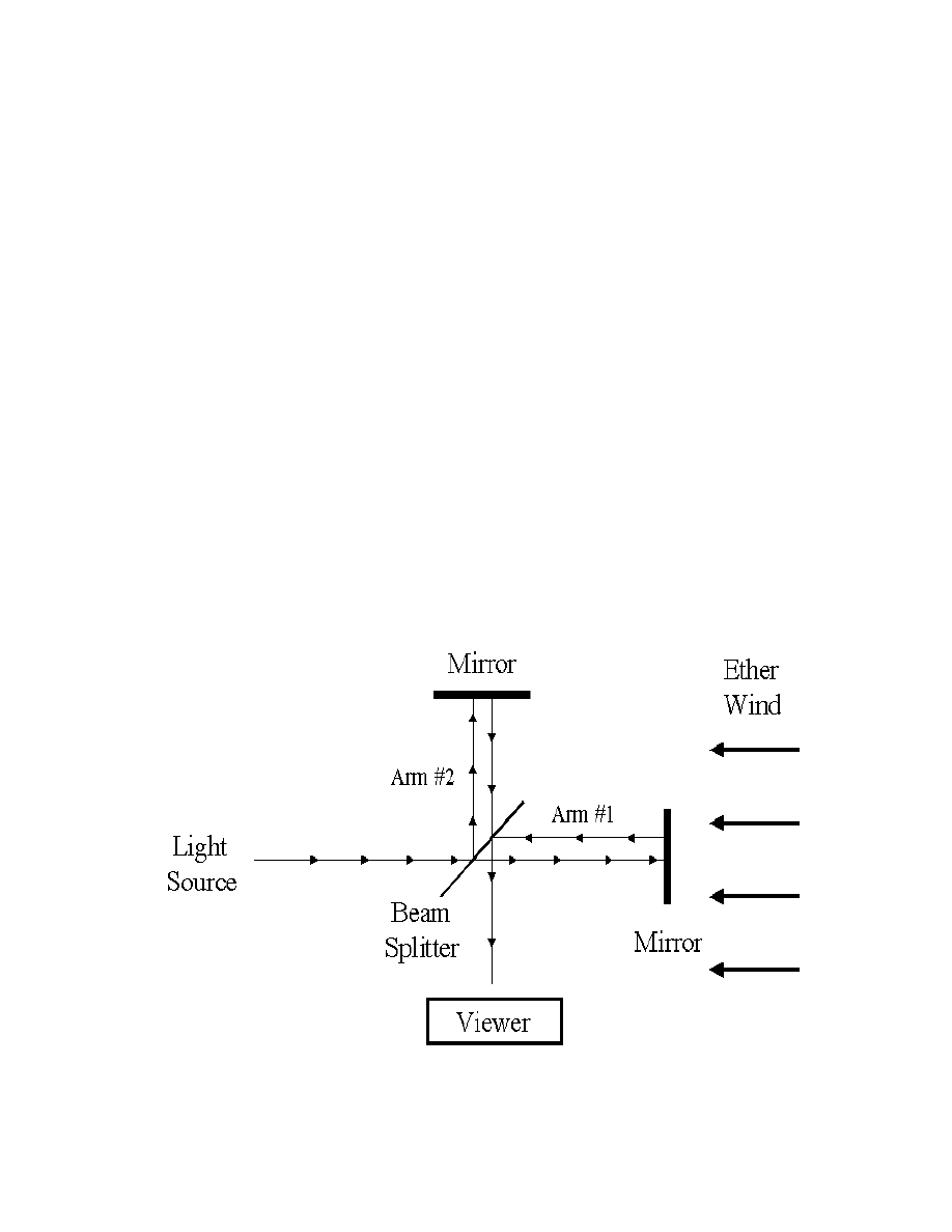
2.2 The Michelson-Morley Experiment
Note. Sound waves need a medium though which to travel. In 1864
James Clerk Maxwell showed that light is an electromagnetic wave.
Therefore it was assumed that there is an ether which propagates light
waves. This ether was assumed to be everywhere and unaffected by
matter. This ether could be used to determine an absolute reference
frame (with the help of observing how light propagates through the
ether).
Note. The Michelson-Morley experiment (circa 1885) was performed
to detect the Earth’s motion through the ether as follows:
The viewer will see the two beams of light which have traveled along
1
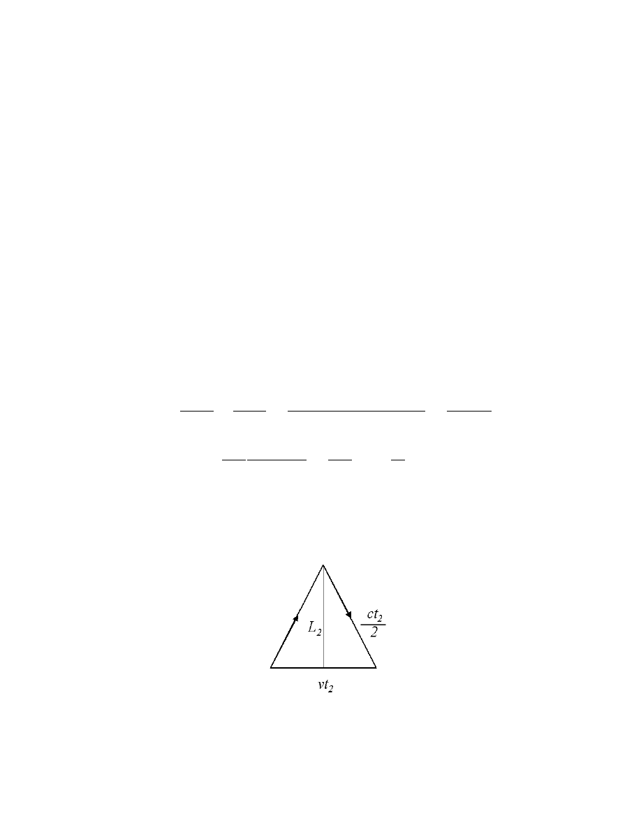
different arms display some interference pattern. If the system is ro-
tated, then the influence of the “ether wind” should change the time
the beams of light take to travel along the arms and therefore should
change the interference pattern. The experiment was performed at
different times of the day and of the year. NO CHANGE IN THE
INTERFERENCE PATTERN WAS OBSERVED!
Example (Exercise 2.2.2). Suppose L
1
is the length of arm #1 and
L
2
is the length of arm#2. The speed of a photon (relative to the
source) on the trip“over” to the mirror is c − v and so takes a time of
L
1
/(c − v). On the return trip, the photon has speed of c + v and so
takes a time of L
1
/(c + v). Therefore the round triptime is
t
1
=
L
1
c − v
+
L
1
c + v
=
L
1
(c + v) + L
1
(c − v)
c
2
− v
2
=
2cL
1
c
2
− v
2
=
2L
1
c
1
1 − v
2
/c
2
=
2L
1
c
1 −
v
2
c
2
−1
.
The photon traveling along arm #2 must follow a path (relative to a
“stationary” observer) of
We need the time the photon travels (t
2
) and the angle at which the
2

photon leaves the mirror to be such that
L
2
2
+
vt
2
2
2
=
ct
2
2
2
(the photon must travel with a component of velocity “upstream” to
compensate for the wind). Then
L
2
2
=
ct
2
2
2
−
vt
2
2
2
L
2
2
= t
2
2
c
2
4
−
v
2
4
t
2
=
2L
2
√
c
2
− v
2
=
2L
2
c
1
1 − v
2
/c
2
Now
1
1 − x
=
∞
n=0
x
n
, so
t
1
≈
2L
1
c
1 +
v
2
c
2
.
Also,
(1 + x)
m
= 1 + mx +
m(m − 1)
2!
x
2
+
m(m − 1)(m − 2)
3!
x
3
+ · · ·
and with m = −1/2 and x = −v
2
/c
2
,
t
2
≈
2L
2
c
1 +
−1
2
−v
2
c
2
=
2L
2
c
1 +
v
2
2c
2
.
For the Earth’s orbit around the sun, v/c ≈ 10
−4
so the approximation
is appropriate. Now the rays recombine at the viewer separated by
∆t = t
1
− t
2
≈
2
c
L
1
− L
2
+
L
1
v
2
c
2
−
L
2
v
2
2c
2
.
Now suppose the apparatus is rotated 90
◦
so that arm #1 is now trans-
verse to the ether wind. Let t
1
and t
2
denote the new round triplight
3
travel times. Then (as above, replacing L
1
with L
2
in t
1
to determine
t
2
and replacing L
2
with L
1
in t
2
to determine t
1
):
t
1
=
2L
1
c
1 +
v
2
2c
2
,
t
2
=
2L
2
c
1 +
v
2
c
2
.
Then
∆t
= t
1
− t
2
=
2
c
(L
1
− L
2
) +
v
2
c
3
(L
1
− 2L
2
)
and
∆t−∆t
=
2
c
(L
1
−L
2
)+
2v
2
c
3
L
1
−
L
2
2
−
2
c
(L
1
− L
2
) +
v
2
c
3
(L
1
− 2L
2
)
=
v
2
c
3
(L
1
+ L
2
).
This is the time change produced by rotating the apparatus.
Note. In 1892, Fitzgerald proposed that an object moving through the
ether wind with velocity v experiences a contraction in the direction of
the ether wind of
1 − v
2
/c
2
. That is, in the diagram above, L
1
is con-
tracted to L
1
1 − v
2
/c
2
and then we get t
1
= t
2
when L
1
= L
2
, p oten-
tially explaining the results of the Michelson-Morley experiment. This
is called the Lorentz-Fitzgerald contraction. Even under this assump-
tion, “it turns out” (see the following example) that the Michelson-
Morley apparatus with unequal arms will exhibit a pattern shift over a
6 month period as the Earth changes direction in its orbit around the
Sun. In 1932, Kennedy and Thorndike performed such an experiment
and detected no such shift.
4
Example (Exercise 2.2.4). Suppose in the Michelson-Morley appa-
ratus that ∆L = L
1
−L
2
= 0 and that there is a contraction by a factor
of
1 − v
2
/c
2
in the direction of the ether wind. Then show
∆t =
2
c
∆L
1 +
v
2
2c
2
.
Solution. As in Exercise 2.2.1, we have
t
1
=
2L
1
c
1
1 − v
2
/c
2
t
2
=
2L
2
c
1
1 − v
2
/c
2
and so
∆t = t
1
− t
2
=
2L
1
c
1
1 − v
2
/c
2
−
2L
2
c
1
1 − v
2
/c
2
=
2
c
(L
1
− L
2
)
1
1 − v
2
/c
2
≈
2
c
(L
1
− L
2
)
1 +
−1
2
−v
2
c
2
=
2
c
(L
1
− L
2
)
1 +
v
2
2c
2
.
Note. Since the equation in the above exercise expresses ∆t as a
function of v only (c, L
1
, and L
2
being constant - although they may
be contracted, but this is taken care of in the computations), we would
see ∆t vary with a period of 6 months (as mentioned above).
Note. Another suggestion to explain the negative result of the Michelson-
Morley experiment was the idea that the Earth “drags the ether along
with it” as it orbits the sun, galactic center, etc. This idea is rejected
because of stellar aberration, discovered by James Bradley in 1725.
5
Example (Exercise 2.2.9). Light rays from a star directly overhead
enter a telescope. Suppose the Earth, in its orbit around the Sun, is
moving at a right angle to the incoming rays, in the direction indicated
in the figure on page 108. In the time it takes a ray to travel down
the barrel to the eyepiece, the telescope will have moved slightly to the
right. Therefore, in order to prevent the light rays from falling on the
side of the barrel rather than on the eyepiece lens, we must tilt the
telescope slightly from the vertical, if we are to see the star. Conse-
quently, the apparent position of the star is displaced forward somewhat
from the actual position. Show that the angle of displacement, θ, is (in
radians)
θ = tan
−1
(v/c) ≈ v/c
where v is the Earth’s orbital velocity. Verify that θ ≈ 20.6
(roughly
the angle subtended by an object 0.1 mm in diameter held at arm’s
length).
Solution. Clearly
θ = tan
−1
v∆t
c∆t
= tan
−1
v
c
.
Now
tan
−1
x =
∞
n=0
(−1)
n
x
2n+1
2n + 1
for |x| < 1
and so tan
−1
v
c
≈
v
c
. We have the Earth’s orbital velocity implying
v/c = 10
−4
(see Exercise 2.2.2). So
θ = 10
−4
= 10
−4
360
◦
2π
60
1
◦
60
1
≈ 20.6
.
6

Note. As the Earth revolves around the Sun in its nearly circular
annual orbit, the apparent position of the star will trace a circle with
angular radius 20.6
. This is indeed observed. If the Earth dragged
a layer of ether along with it, the light rays, upon entering this layer,
would aquire a horizontal velocity component matching the forward
velocity v of the telescope. There would then be no aberration effect.
Conclusion. The speed of light is constant and the same in all direc-
tions and in all inertial frames.
7

2.3 The Postulates of Relativity
Note. Albert Einstein published “Zur Elektrodynamik bewegter K¨orper”
(On the Electrodynamics of Moving Bodies) in Annalen der Physik (An-
nals of Physics) 17 (1905). In this paper, he established the SPECIAL
THEORY OF RELATIVITY! I quote (from “The Principles of
Relativity” by H. A. Lorenz, A. Einstein, H. Minkowski, and H. Weyl,
published by Dover Publications):
“...the same laws of electrodynamics and optics will be valid
for all frames of reference for which the equations of me-
chanics hold good. We raise this conjecture (the purport of
which will hereafter be called the “Principle of Relativity”)
to the status of a postulate, and also introduce another
postulate, which is only apparently irreconcilable with the
former, namely, that light is always propagated in empty
space with a definite velocity c which is independent of the
state of motion of the emitting body.”
In short:
P1. All physical laws valid in one frame of reference are equally valid
in any other frame moving uniformly relative to the first.
P2. The speed of light (in a vacuum) is the same in all inertial frames
of reference, regardless of the motion of the light source.
From these two simple (and empirically varified) assumptions arises the
beginning of the revolution that marks our transition from classical to
modern physics!
1
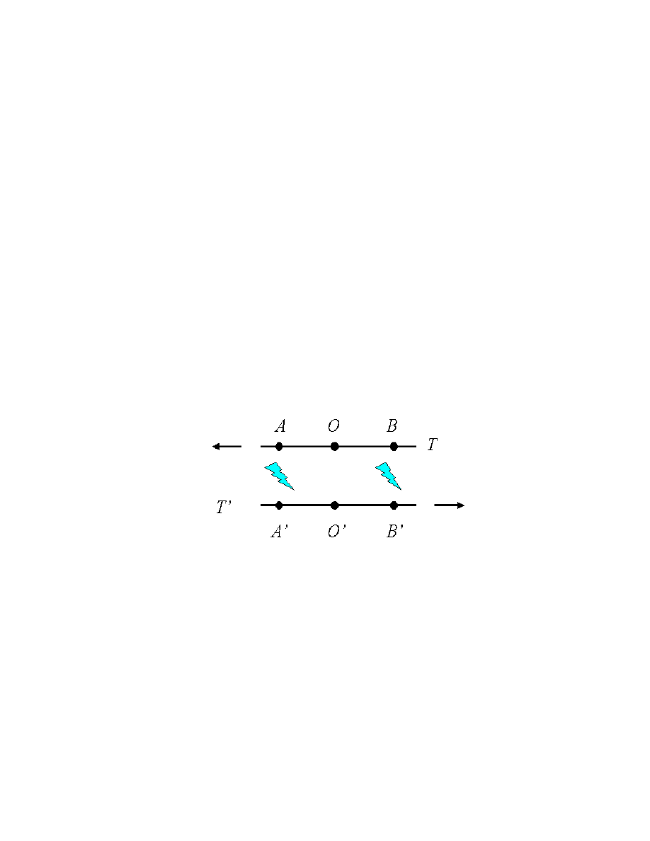
2.4 Relativity of Simultaneity
Note. Suppose two trains T and T
pass each other traveling in op-
posite directions (this is equivalent to two inertial frames moving uni-
formly relative to one another). Also suppose there is a flash of lighten-
ing (an emission of light) at a certain point (see Figure II-3). Mark the
points on trains T and T
where this flash occurs at A and A
respec-
tively. “Next,” suppose there is another flash of lightning and mark
the points B and B
. Suppose point O on train T is midway between
points A and B, AND that point O
on train T
is midway between
points A
and B
. An outsider might see:
Suppose an observer at point O sees the flashes at points A and B occur
at the same time. From the point of view of O the sequence of events
is:
1
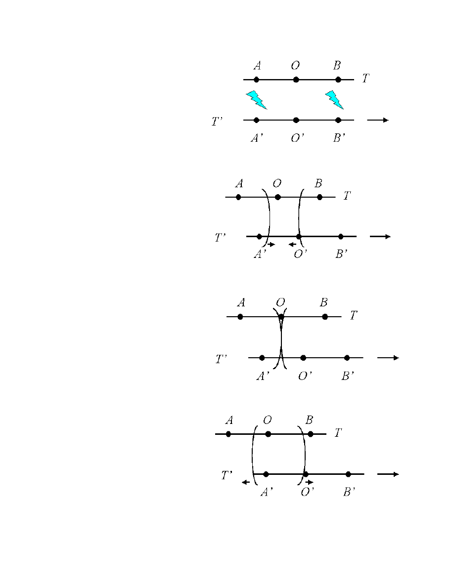
(1) Both flashes occur,
A, O, B opposite
A
, O
, B
, resp.
(2) Wavefront from
BB
meets O
(3) Both wavefronts
meet O
(4) Wavefront from
AA
meets O
2
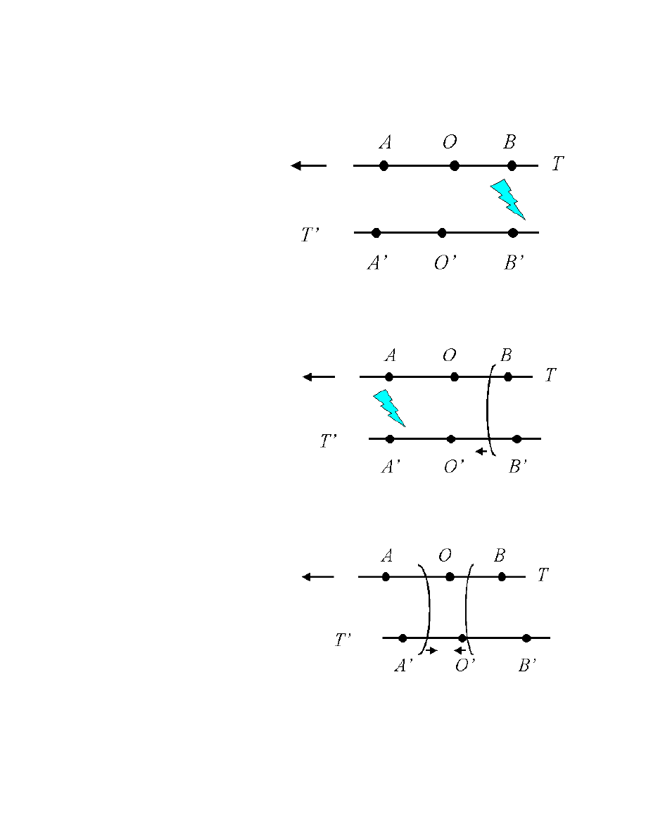
From the point of view of an observer at O
, the following sequence of
events are observed:
(1) Flash occurs
at BB
(2) Flash occurs
at AA
(3) Wavefront from
BB
meets O
3
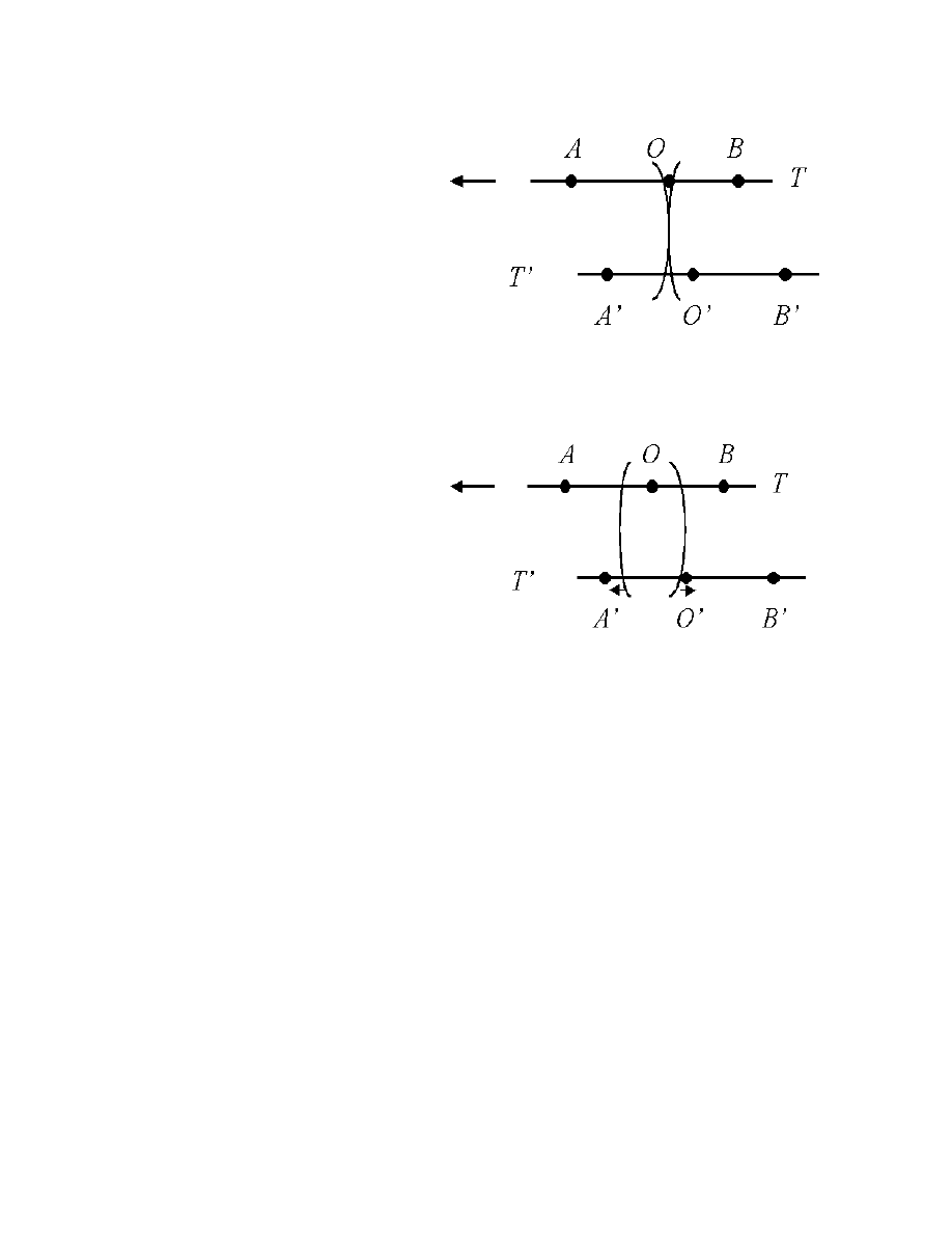
(4) Wavefronts from
AA
and BB
meet O
(5) Wavefront from
AA
meets O
Notice that the speed of light is the same in both frames of reference.
However, the observer on train T sees the flashes occur simultaneously,
whereas the observer on train T
sees the flash at BB
occur before the
flash at AA
. Therefore, events that appear to be simultaneous in one
frame of reference, may not appear to be simultaneous in another. This
is the relativity of simultaneity.
4

Note. The relativity of simultaneity has implications for the mea-
surements of lengths. In order to measure the length of an object, we
must measure the position of both ends of the object simultaneously.
Therefore, if the object is moving relative to us, there is a problem.
In the above example, observer O sees distances AB and A
B
equal,
but observer O
sees AB shorter than A
B
. Therefore, we see that
measurements of lengths are relative!
5

2.5 Coordinates
Definition. In 3-dimensional geometry, positions are represented by
points (x, y, z). In physics, we are interested in events which have both
time and position (t, x, y, z). The collection of all possible events is
spacetime.
Definition. With an event (t, x, y, z) in spacetime we associate the
units of cm with coordinates x, y, z. In addition, we express t (time) in
terms of cm by multiplying it by c. (In fact, many texts use coordinates
(ct, x, y, z) for events.) These common units (cm for us) are called
geometric units.
Note. We express velocities in dimensionless units by dividing them
by c. S o for velocity v (in cm/sec, say) we associate the dimensionless
velocity β = v/c. Notice that under this convention, the speed of light
is 1.
Note. In an inertial frame S, we can imagine a grid laid out with a
clock at each point of the grid. The clocks can by synchronized (see
page 118 for details). When we mention that an object is observed in
frame S, we mean that all of its parts are measured simultaneously
(using the synchronized clocks). This can be quite different from what
an observer at a point actually sees.
Note. From now on, when we consider two inertial frames S and S
1
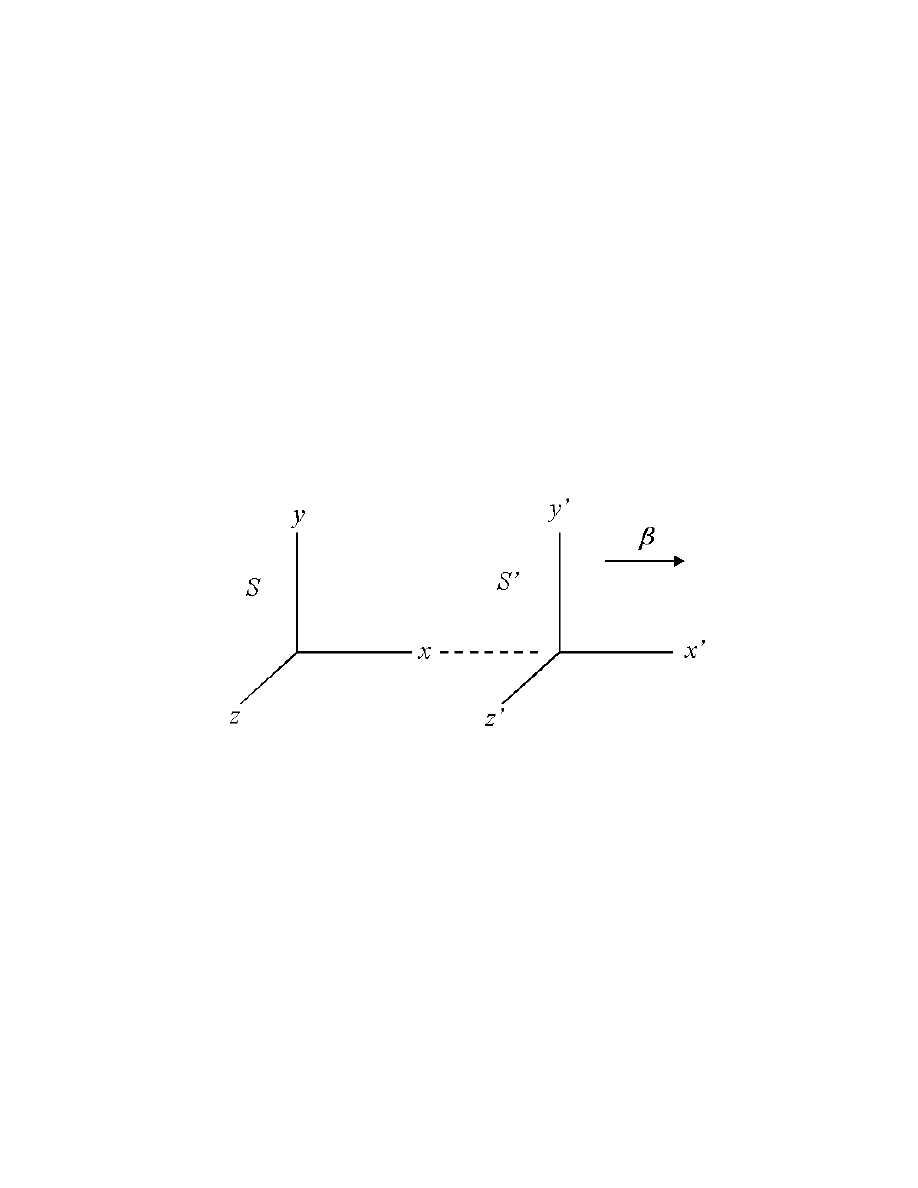
moving uniformly relative to each other, we adopt the conventions:
1. The x− and x
−axes (and their positive directions) coincide.
2. Relative to S, S
is moving in the positive x direction with velocity
β.
3. The y− and y
−axes are always parallel.
4. The z− and z
−axes are always parallel.
We call S the laboratory frame and S
the rocket frame:
Assumptions. We assume space is homogeneous and isotropic, that
is, space appears the same at all points (on a sufficiently large scale)
and appears the same in all directions.
Lemma. Suppose two inertial frames S and S
move uniformly relative
to each other. Then lengths perpendicular to the direction of motion
are the same for observers in both frames (that is, under our convention,
there is no length contraction or expansion in the y or z directions).
2
Proof. Suppose there is a right circular cylinder C of radius R (as
measured in S) with its axis along the x−axis. Similarly, suppose there
is a right circular cylinder C
of radius R
(as measured in S
) with its
axis lying along the x
−axis. Suppose the cylinders are the same radius
when “at rest.” Since space is assumed to be isotropic, each observer
will see a circular cylinder in the other frame (or else, there would be
directional asymmetry to space). Now suppose the lab observer (S)
measures a smaller radius r < R for cylinder C
. Then he will see
cylinder C
pass through the interior of his cylinder C (see Figure II-7,
page 120). Now if two points are coincident (at the same place) in one
inertial frame, then they must be coincident in another inertial frame
(they are, after all, at the same place). So if the lab observer sees C
inside C, then the rocket observer must see this as well. However, by
the Principle of Relativity (P
1
), the rocket observer must see C inside
C
. This contradiction yields r ≥ R. Similarly, there is a contradiction
if we assume r > R. Therefore, r = R and both observers see C and
C
as cylinders with radius R. Therefore, there is no length change in
the y or z directions.
Note. In the next section, we’ll see that things are much different in
the direction of motion.
3
2.6 Invariance of the Interval
Note. In this section, we define a quantity called the “interval” be-
tween two events which is invariant under a change of spacetime coor-
dinates from one inertial frame to another (analogous to “distance” in
geometry). We will also derive equations for time and length dilation.
Note. Consider the experiment described in Figure II-8. In inertial
frame S
a beam of light is emitted from the origin, travels a distance
L, hits a mirror and returns to the origin. If ∆t
is the amount of time
it takes the light to return to the origin, then L = ∆t
/2 (recall that t
is multiplied by c in order to put it in geometric units). An observer in
frame S sees the light follow the path of Figure II-8b in time ∆t. Notice
that the situation here is not symmetric since the laboratory observer
requires two clocks (at two positions) to determine ∆t, whereas the
rocket observer only needs one clock (so the Principle of Relativity does
not apply). In geometric units, we have: (∆t/2)
2
= (∆t
/2)
2
+ (∆x/2)
2
or (∆t
)
2
= (∆t)
2
− (∆x)
2
with β the velocity of S
relative to S, we
have β = ∆x/∆t and so ∆x = β∆t and (∆t
)
2
= (∆t)
2
− (β∆t)
2
or
∆t
=
1 − β
2
∆t.
(78)
Therefore we see that under the hypotheses of relativity, time is not
absolute and the time between events depends on an observer’s motion
relative to the events.
1
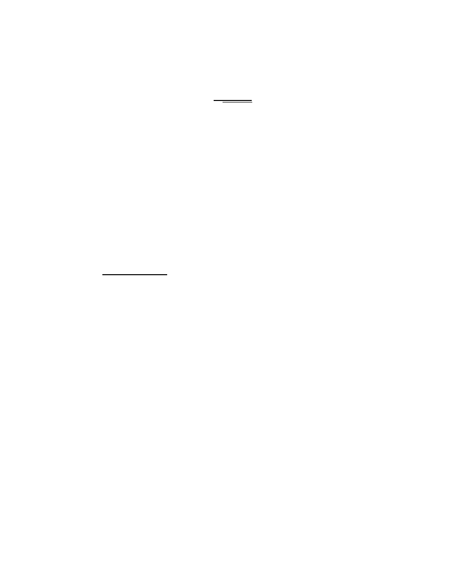
Note. You might be more familiar with equation (78) in the form:
∆t =
1
√
1 − β
2
∆t
where ∆t
is an interval of time in the rocket frame and ∆t is how the
laboratory frame measures this time interval. Notice ∆t ≥ ∆t
so that
time is dilated (lengthened).
Note. Since β = v/c, for v c, β ≈ 0 and ∆t
≈ ∆t.
Definition. Suppose events A and B occur in inertial frame S at
(t
1
, x
1
, y
1
, z
1
) and (t
2
, x
2
, y
2
, z
2
), respectively, where y
1
= y
2
and z
1
=
z
2
. Then define the interval (or proper time) between A and B as
∆τ =
(∆t)
2
− (∆x)
2
where ∆t = t
2
− t
1
and ∆x = x
2
− x
1
.
Note. As shown above, in the S
frame
(∆t
)
2
− (∆x
)
2
= (∆t)
2
− (∆x)
2
(recall ∆x
= 0). So ∆τ is the same in S
. That is, the interval is
invariant from S to S
. As the text says “The interval is to spacetime
geometry what the distance is to Euclidean geometry.”
Note. We could extend the definition of interval to motion more com-
plicated than motion along the x−axis as follows:
∆τ = {(∆t)
2
− (∆x)
2
− (∆y)
2
− (∆z)
2
}
1/2
or
(interval)
2
= (time separation)
2
− (space separation)
2
.
2
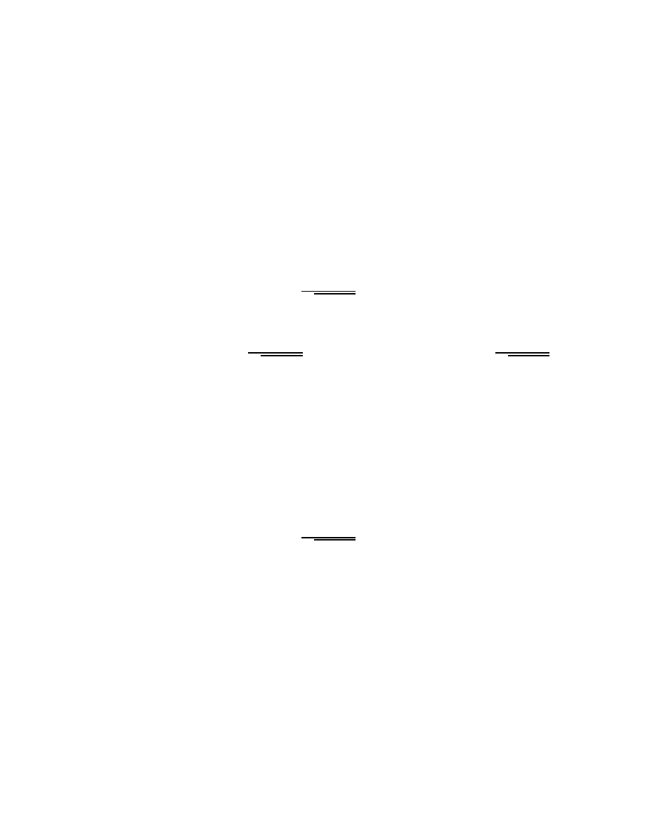
Note. Let’s explore this “time dilation” in more detail. In our example,
we have events A and B occuring in the S
frame at the same position
(∆x
= 0), but at different times. Suppose for example that events A
and B are separated by one time unit in the S
frame (∆t
= 1). W e
could then represent the ticking of a second hand on a watch which is
stationary in the S
frame by these two events. An observer in the S
frame then measures this ∆t
= 1 as
∆t =
1
√
1 − β
2
∆t
.
That is, an observer in the S frame sees the one time unit stretched
(dilated) to a length of
1
√
1 − β
2
≥ 1 time unit. So the factor
1
√
1 − β
2
shows how much slower a moving clock ticks in comparison to a sta-
tionary clock. The Principle of Relativity implies that on observer in
frame S
will see a clock stationary in the S frame tick slowly as well.
However, the Principle of Relativity does not apply in our example
above (see p. 123) and both an observer in S and an observer in S
agree that ∆t and ∆t
are related by
∆t =
1
√
1 − β
2
∆t
.
So both agree that ∆t ≥ ∆t
in this case. This seems strange ini-
tially, but will make more sense when we explore the interval below.
(Remember, ∆x = 0.)
3
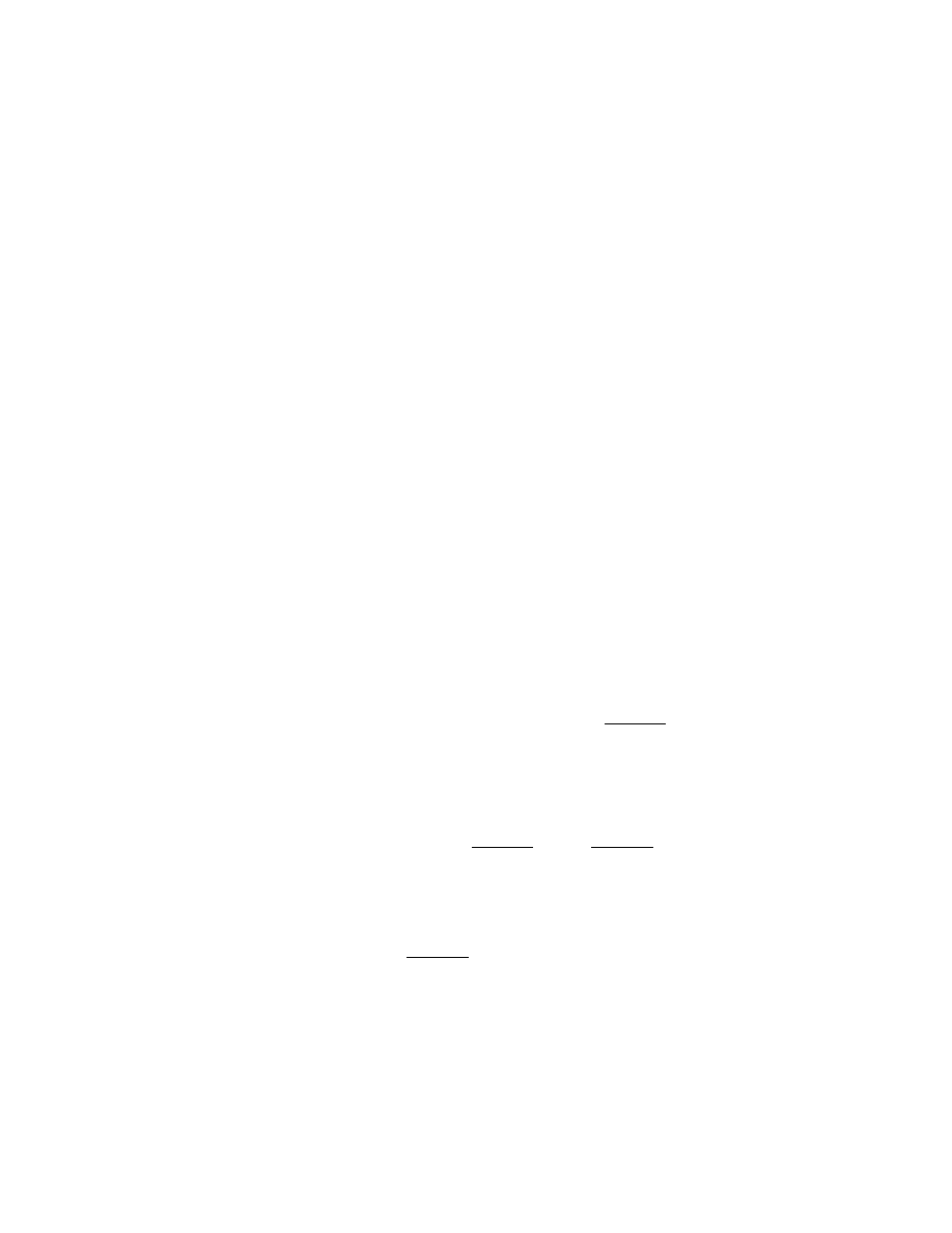
Definition. An interval in which time separation dominates and (∆τ )
2
>
0 is timelike. An interval in which space separation dominates and
(∆τ )
2
< 0 is spacelike. An interval for which ∆τ = 0 is lightlike.
Note. If it is possible for a material particle to be present at two events,
then the events are separated by a timelike interval. No material object
can be present at two events which are separated by a spacelike interval
(the particle would have to go faster than light). If a ray of light can
travel between two events then the events are separated by an interval
which is lightlike. We see this in more detail when we look at spacetime
diagrams (Section 2.8).
Note. If an observer in frame S
passes a “platform” (all the train talk
is due to Einstein’s original work) of length L in frame S at a speed of
β, then a laboratory observer on the platform sees the rocket observer
pass the platform in a time ∆t = L/β. As argued above, the rocket
observer measures this time period as ∆t
= ∆t
√
1 − β
2
. Therefore, the
rocket observer sees the platform go by in time ∆t
and so measures
the length of the platform as
L
= β∆t
= β∆t
1 − β
2
= L
1 − β
2
.
Therefore we see that the time dilation also implies a length contraction:
L
= L
1 − β
2
.
(83)
4
Note. Equation (83) implies that lengths are contracted when an ob-
ject is moving fast relative to the observer. Notice that with β ≈ 0,
L
≈ L.
Example (Exercise 2.6.2). Pions are subatomic particles which de-
cay radioactively. At rest, they have a half-life of 1.8 × 10
−8
sec. A pion
beam is accelerated to β = 0.99. According to classical physics, this
beam should drop to one-half its original intensity after traveling for
(0.99)(3 × 10
8
)(1.8 × 10
−8
) ≈ 5.3m. However, it is found that it drops
to about one-half intensity after traveling 38m. Explain, using either
time dilation or length contraction.
Solution. Time is not absolute and a given amount of time ∆t
in
one inertial frame (the pion’s frame, say) is observed to be dilated in
another inertial frame (the particle accelerator’s) to ∆t = ∆t
/
√
1 − β
2
.
So with ∆t
= 1.8 × 10
−8
sec and β = 0.99,
∆t =
1
√
1 − .99
2
(1.8 × 10
−8
sec) = 1.28 × 10
−7
sec.
Now with β = .99, the speed of the pion is (.99)(3 × 10
8
m/sec) =
2.97 × 10
8
m/sec and in the inertial frame of the accelerator the pion
travels
(2.97 × 10
8
m/sec)(1.28 × 10
−7
sec) = 38m.
In terms of length contraction, the accelerator’s length of 38m is con-
tracted to a length of
L
= L
1 − β
2
= (38m)
√
1 − .99
2
= 5.3m
5

in the pion’s frame. With v = .99c, the pion travels this distance in
5.3m
(.99)(3 × 10
8
m/sec)
= 1.8 × 10
−8
sec.
This is the half-life and therefore the pion drops to 1/2 its intensity
after traveling 38m in the accelerator’s frame.
6

2.7 The Lorentz Transformation
Note. We seek to find the transformation of the coordinates (x, y, z, t)
in an inertial frame S to the coordinates (x
, y
, z
, t
) in inertial frame
S
. Throughout this section, we assume the x and x
axes coincide, S
moves with velocity β in the direction of the positive x axis, and the
origins of the systems coincide at t = t
= 0. See Figure II-9, page 128.
Note. Classically, we have the relations
x = x
+ βt
y = y
z = z
t = t
Definition. The assumption of homogeneity says that there is no pre-
ferred location in space (that is, space looks the same at all points [on
a sufficiently large scale]). The assumption of isotropy says that there
is no preferred direction in space (that is, space looks the same in every
direction).
Note. Under the assumptions of homogeneity and isotropy, the rela-
tions between (x, y, z, t) and (x
.y
, z
, t
) must be linear (throughout,
everything is done in geometric units!):
1

x = a
11
x
+ a
12
y
+ a
13
z
+ a
14
t
y = a
21
x
+ a
22
y
+ a
23
z
+ a
24
t
z = a
31
x
+ a
32
y
+ a
33
z
+ a
34
t
t = a
41
x
+ a
42
y
+ a
43
z
+ a
44
t
.
If not, say y = ax
2
, then a rod lying along the x−axis of length x
b
− x
a
would get longer as we moved it out the x−axis, contradicting homo-
geneity. Similarly, relationships involving time must be linear (since the
length of a time interval should not depend on time itself, nor should
the length of a spatial interval).
Note. We saw in Section 2.5 that lengths perpendicular to the direction
of motion are invariant. Therefore
y = y
z = z
Note. x does not depend on y
and z
. Suppose not. Suppose there is a
flat plate at rest in S
and perpendicular to the x
−axis. Since the above
equations are linear, an observer in S would see the plate tilted (but still
flat) if there is a dependence on y
or z
. However, this implies a “special
direction” in space violating the assumption of isotropy. Therefore, the
coefficients a
12
and a
13
are 0. Similarly, isotropy implies a
42
= a
43
= 0.
We have reduced the system of equations to
x = a
11
x
+ a
14
t
(85)
t = a
41
x
+ a
44
t
(86)
2
Note. Recall Figure II-8, page 122. A beam of light is emitted from
the origin of S
at time t = t
= 0 (when x = x
= 0), bounced off a
mirror and reflected back to the S
origin (x
= 0) at time t
= ∆t
. In
S, the light returns to the origin (x
= 0) at time t = ∆t = 1/
√
1 − β
2
t
(equation (78), page 123). Also, in S with x
= 0 we have (from
equation (86)) that t = a
44
t
. Therefore a
44
= 1/
√
1 − β
2
. Next, with
x
= 0 and t = t
/
√
1 − β
2
, since the point x
= 0 occurs in the S frame
at x = βt (due to the relative motion), we have from equation (85):
x = βt =
β
√
1 − β
2
t
= a
14
t
and so a
14
=
β
√
1 − β
2
. So equations (85) and (86) give
x = a
11
x
+
β
√
1 − β
2
t
(87)
t = a
41
x
+
1
√
1 − β
2
t
(88)
Note. Now consider a flash of light emitted at the origins of S and S
at t = t
= 0. This produces a sphere of light in each frame (according
to the constancy of the speed of light). And so
t
2
= x
2
+ y
2
+ z
2
t
2
= x
2
+ y
2
+ z
2
.
Since y = y
and z = z
, we have t
2
− x
2
= t
2
− x
2
. From equations
(87) and (88) we get
t
2
− x
2
=
a
41
x
+
1
√
1 − β
2
t
2
−
a
11
x
+
β
√
1 − β
2
t
2
= t
2
− x
2
.
3
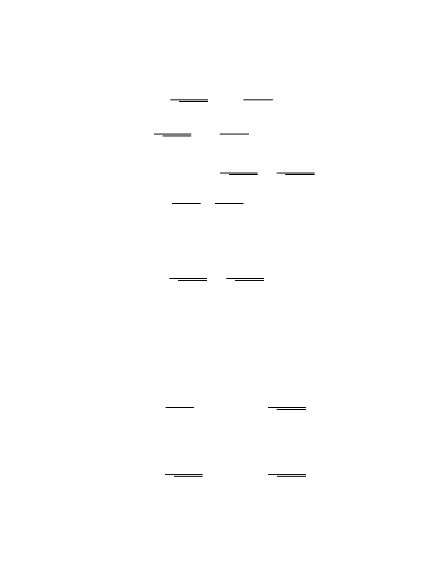
Expanding
(a
41
)
2
x
2
+
2a
41
√
1 − β
2
x
t
+
1
1 − β
2
t
2
− (a
11
)
2
x
2
−2
a
11
β
√
1 − β
2
x
t
−
β
2
1 − β
2
t
2
= t
2
− x
2
or
x
2
(a
2
41
− a
2
11
) + x
t
2a
41
√
1 − β
2
− 2
a
11
β
√
1 − β
2
+t
2
1
1 − β
2
−
β
2
1 − β
2
= t
2
− x
2
.
Comparing coefficients, we need
a
2
41
− a
2
11
= −1
2
a
41
√
1 − β
2
− 2
a
11
β
√
1 − β
2
= 0
or
a
2
41
− a
2
11
= −1 and a
41
− βa
11
= 0.
Solving this system: a
41
= βa
11
and so
a
2
41
− a
2
11
= (βa
11
)
2
− a
2
11
= −1
or
a
2
11
=
1
1 − β
2
and a
11
= ±
1
√
1 − β
2
.
From equation (87) with β = 0 we see that x =
a
11
|
β=0
x
and we
want x = x
in the event that β = 0. Therefore, we have
a
11
=
1
√
1 − β
2
and a
41
=
β
√
1 − β
2
.
We now have the desired relations between (x, y, z, t) and (x
, y
, z
, t
).
4
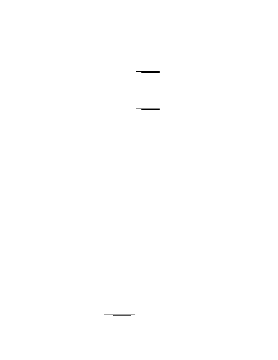
Definition. The transformation relating coordinates (x, y, z, t) in S to
coordinates (x
, y
, z
, t
) in S
given by
x =
x
+ βt
√
1 − β
2
y = y
z = z
t =
βx
+ t
√
1 − β
2
is called the Lorentz Transformation.
Note. With β 1 and β
2
≈ 0 we have
x = x
+ βt
t = t
(in geometric units, x and x
are small compared to t and t
[see page
117 - remember time gets multiplied by c to express it in units of length]
and βx
is negligible compared to t
, but βt
is NOT negligible compared
to x
).
Note. By the Principle of Relativity, we can invert the Lorentz Trans-
formation simply by interchanging x and t with x
and t
, respectively,
and replacing β with −β!
Note. If we deal with pairs of events separated in space and time, we
denote the differences in coordinates with ∆’s to get
∆x =
∆x
+ β∆t
√
1 − β
2
(91a)
5
∆t =
β∆x
+ ∆t
√
1 − β
2
(91b)
With ∆x
= 0 in (91b) we get the equation for time dilation. With a
rod of length L = ∆x in frame S, the length measured in S
requires a
simultaneous measurement of the endpoints (∆t
= 0) and so from (91a)
L = L
/
√
1 − β
2
or L
= L
√
1 − β
2
, the equation for length contraction.
Example (Exercise 2.7.2). Observer S
seated at the center of a
railroad car observes two men, seated at opposite ends of the car, light
cigarettes simultaneously (∆t
= 0). However for S, an observer on the
station platform, these events are not simultaneous (∆t = 0). If the
length of the railroad car is ∆x
= 25m and the speed of the car relative
to the platform is 20m/sec (β = 20/3 × 10
8
), find ∆t and convert your
answer to seconds.
Solution. We have ∆t
= 0, ∆x
= 25m, and β = 20/3 × 10
8
≈
6.67 × 10
−8
. So by equation (91b)
∆t =
β∆x
+ ∆t
√
1 − β
2
=
(6.67 × 10
−8
)(25m)
1 − (6.67 × 10
−8
)
2
≈ 1.67 × 10
−6
m
or in seconds
∆t =
1.67 × 10
−6
m
3 × 10
8
m/sec
= 5.56 × 10
−15
sec.
6
Example (Exercise 2.7.14). Substitute the transformation Equation
(91) into the formula for the interval and verify that
(∆t)
2
− (∆x)
2
− (∆y)
2
− (∆z)
2
= (∆t
)
2
− (∆x
)
2
− (∆y
)
2
− (∆z
)
2
.
Solution. With ∆y = ∆z = 0 we have
(∆t)
2
−(∆x)
2
− (∆y)
2
− (∆z)
2
=
(∆t)
2
− (∆x)
2
=
β∆x
+ ∆t
√
1 − β
2
2
−
∆x
+ β∆t
√
1 − β
2
2
=
β
2
(∆x
)
2
+ 2β∆x
∆t
+ (∆t
)
2
− (∆x
)
2
− 2β∆x
∆t
− β
2
(∆t
)
2
1 − β
2
=
(∆x
)
2
(β
2
− 1) + (∆t
)
2
(1 − β
2
)
1 − β
2
=
(∆t
)
2
− (∆x
)
2
= (∆t
)
2
− (∆x
)
2
− (∆y
)
2
− (∆z
)
2
since ∆y
= ∆z
= 0.
7
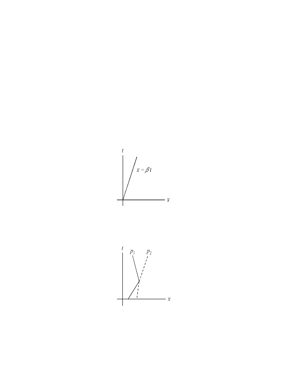
2.8 Spacetime Diagrams
Note. We cannot (as creatures stuck in 3 physical dimensions) draw
the full 4 dimensions of spacetime. However, for rectilinear or planar
motion, we can depict a particle’s movement. We do so with a spacetime
diagram in which spatial axes (one or two) are drawn as horizontal axes
and time is represented by a vertical axis. In the xt−plane, a particle
with velocity β is a line of the form x = βt (a line of slope 1/β):
Two particles with the same spacetime coordinates must be in collision:
1
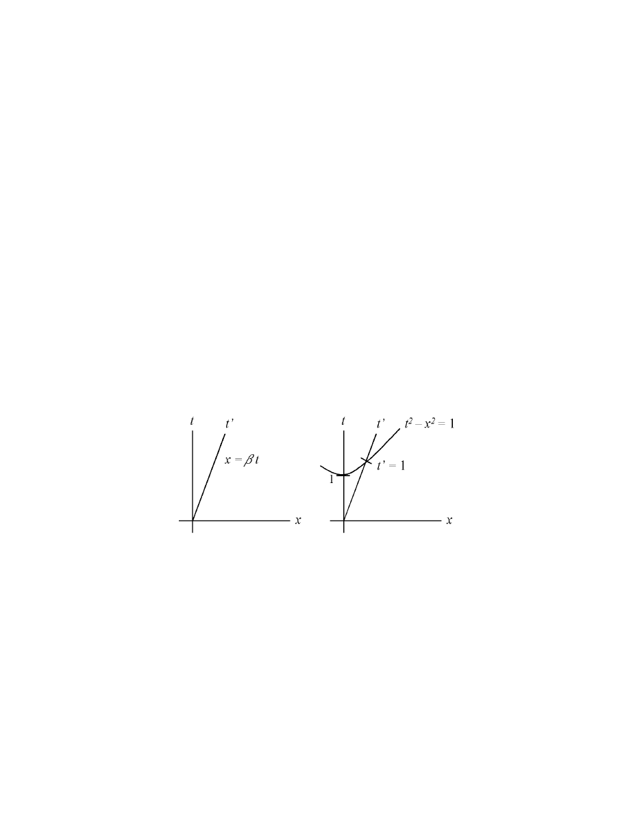
Note. The picture on the cover of the text is the graph of the orbit of
the Earth as it goes around the Sun as plotted in a 3-D spacetime.
Definition. The curve in 4-dimensional spacetime which represents the
relationships between the spatial and temporal locations of a particle
is the particle’s world-line.
Note. Now let’s represent two inertial frames of reference S and S
(considering only the xt−plane and the x
t
−plane). Draw the x and t
axes as perpendicular (as above). If the systems are such that x = 0
and x
= 0 coincide at t = t
= 0, then the point x
= 0 traces out the
path x = βt in S. We define this as the t
axis:
The hyperbola t
2
−x
2
= 1 in S is the same as the “hyperbola” t
2
−x
2
=
1 in S
(invariance of the interval). So the intersection of this hyperbola
and the t
axis marks one time unit on t
. Now from equation (90b)
(with t
= 0) we get t = βx and define this as the x
axis. Again we
2
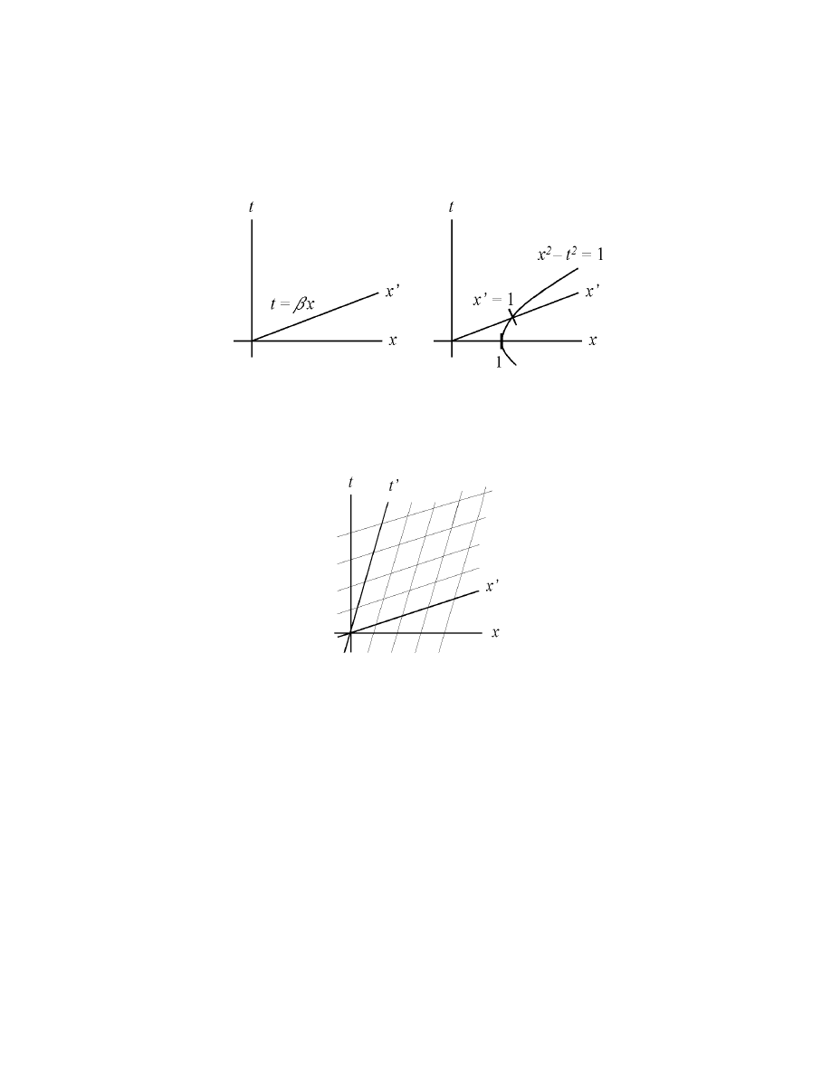
calibrate this axis with a hyperbola (x
2
− t
2
= 1):
We therefore have:
and so the S
coordinate system is oblique in the S spacetime diagram.
Note. In the above representation, notice that the larger β is, the more
narrow the “first quadrant” of the S
system is and the longer the x
and t
units are (as viewed from S).
Note. Suppose events A and B are simultaneous in S
They need not
be simultaneous in S. Events C and D simultaneous in S need not be
3
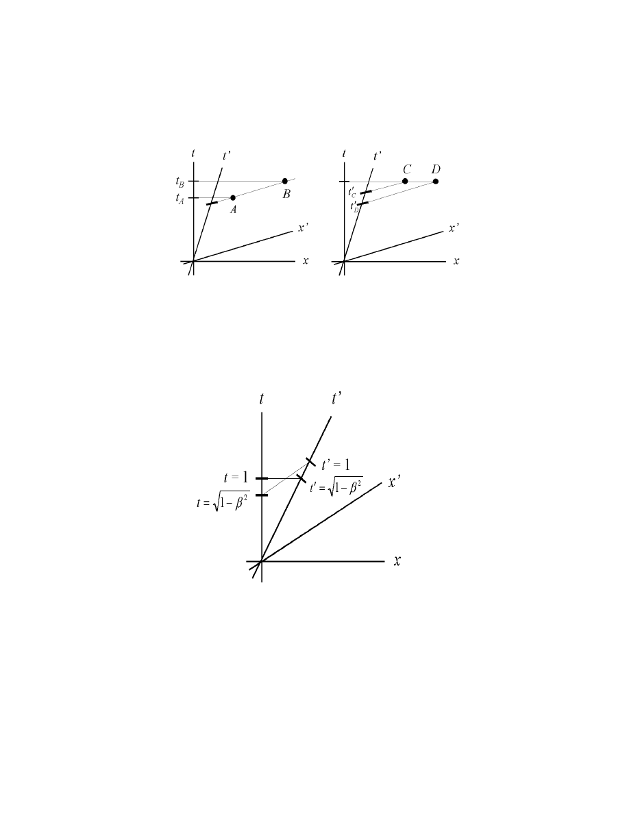
simultaneous in S
.
Note. A unit of time in S is dilated in S
and a unit of time in S
is
dilated in S.
Note. Suppose a unit length rod lies along the x axis. If its length
is measured in S
(the ends have to be measured simultaneously in S
)
4
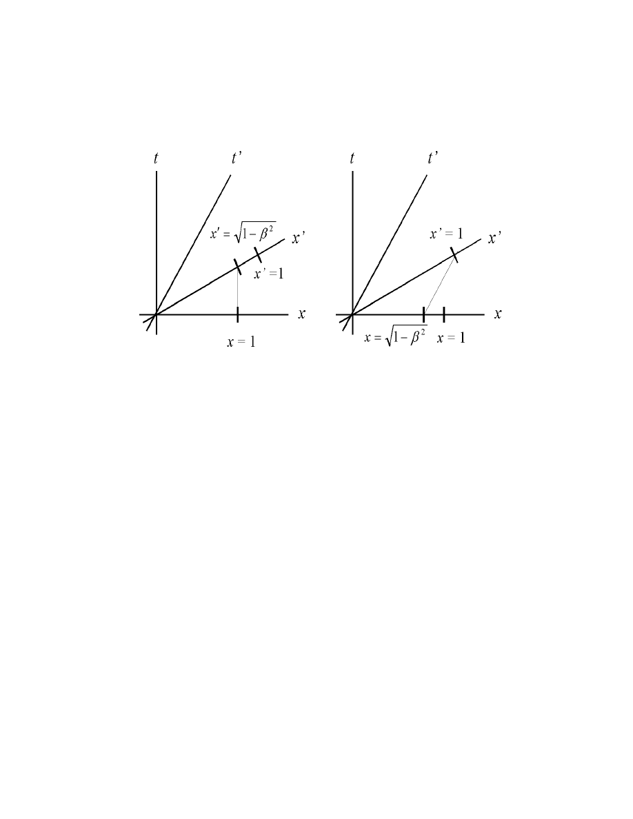
then the rod is shorter. Conversely for rods lying along the x
axis.
Example (Exercise 2.8.4). An athlete carrying a pole 16m long runs
toward the front door of a barn so rapidly that an observer in the barn
measures the pole’s length as only 8m, which is exactly the length of
the barn. Therefore at some instant the pole will be observed entirely
contained within the barn. Suppose that the barn observer closes the
front and back doors of the barn at the instant he observes the pole
entirely contained by the barn. What will the athlete observe?
Solution. We have two events of interest:
A = The front of the pole is at the back of the barn.
B = The back of the pole is at the front of the barn.
From Exercise 2.8.3, the observer in the barn (frame S) observes these
events as simultaneous (each occuring at t
AB
= 3.08 × 10
−8
sec after the
5
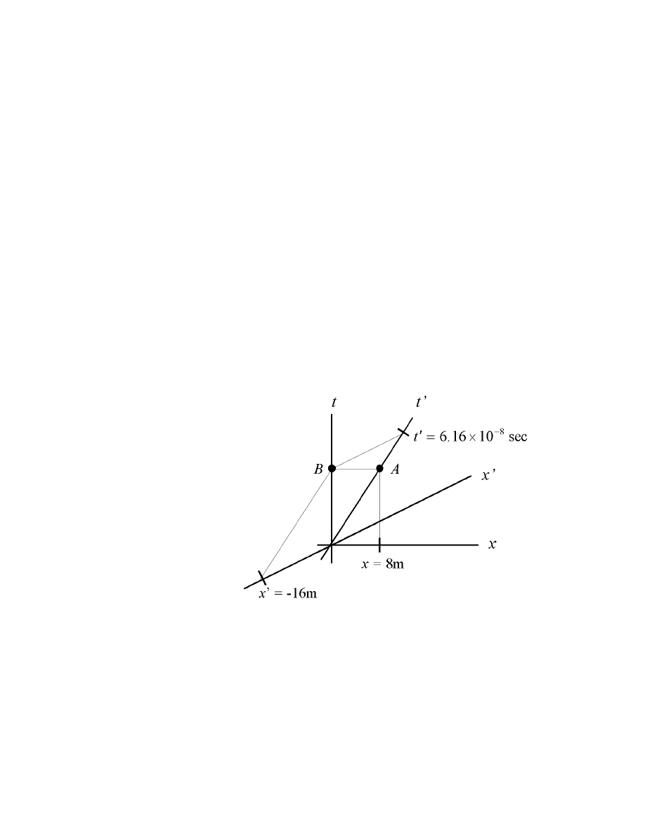
front of the pole was at the front of the barn). However, the athlete
observes event A after he has moved the pole only 4m into the barn.
So for him, event A occurs when t
A
= 1.54 × 10
−8
sec. Event B does not
occur until the pole has moved 16m (from t
= 0) and so event B occurs
for the athlete when t
B
= 6.16 × 10
−8
sec. Therefore, the barn observer
observes the pole totally within the barn (events A and B), slams the
barn doors, and observes the pole start to break through the back of
the barn all simultaneously. The athlete first observes event A along
with the slamming of the back barn door and the pole starting to break
through this door (when t
= 1.54 × 10
−8
sec) and THEN observes the
front barn door slam at t
B
= 6.16 × 10
−8
sec. The spacetime diagram
is:
A occurs at
t
= 1.54 × 10
−8
sec
B occurs at
t = 3.08 × 10
−8
sec
Since the order of events depends on the frame of reference, the appar-
ent paradox is explained.
Example (Exercise 2.8.5). Using a diagram similar to Figure II-15,
show that (a) at time t = 0 in the laboratory frame, the rocket clocks
6
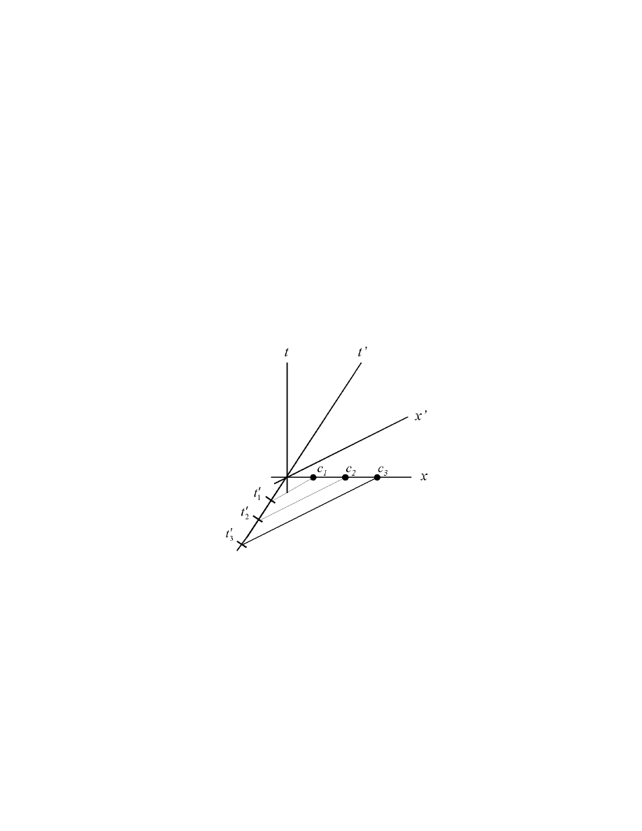
that lie along the positive x−axis are observed by S to be set behind
the laboratory clocks, with the clocks further from the origin set further
behind, and that (b) at time t
= 0 in the rocket frame, the laboratory
clocks that lie along the positive x
−axis are observed by S
to be set
further ahead.
Solution. (a) At t = 0, clocks in S
that lie along the positive x−axis
are observed by S to be behind the S clocks, with the clocks further
from the origin set further behind:
So clocks c
i
arranged as in the figure read times 0 > t
1
> t
2
> t
3
> · · ·.
7
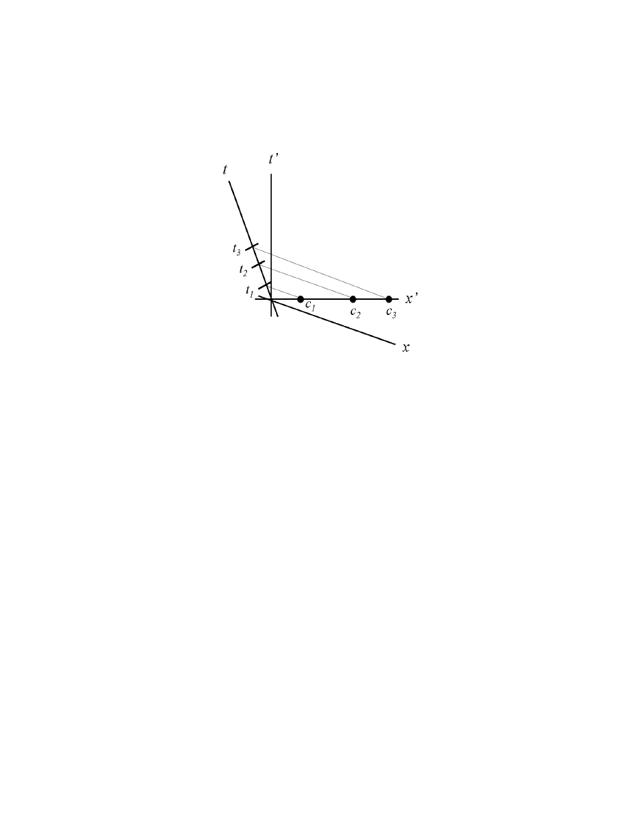
(b) Conversely, in the S
frame:
So clocks c
i
arranged as in the figure read times 0 < t
1
< t
2
< t
3
< · · ·.
8
2.9 Lorentz Geometry
Note. We wish to extend the idea of arclength to 4-dimensional space-
time. We do so by replacing the idea of “distance” (
(∆x
i
)
2
) by the
interval. The resulting geometry is called Lorentz geometry.
Definition. Let α be a curve in spacetime. The spacetime length (or
proper time) of α is
L(α) −
α
dτ =
α
(dt)
2
− (dx)
2
− (dy)
2
− (dz)
2
.
Note. Since ∆τ (and so dτ ) is an invariant from one inertial frame to
another, then so is L(α). L(α) may be viewed as the actual passage
of time that would be recorded for a clock with world-line α (this is
certainly clear when dx = dy = dz = 0).
Definition. R
4
with the semi-Riemannian metric
dτ
2
= (dt)
2
− (dx)
2
− (dy)
2
− (dz)
2
(93)
is called Minkowski space. (This may seem a bit unusual to see (dτ )
2
referred to as the “metric,” but of course it does determine a way
to measure the distance between points - although the square of this
“distance” may be negative).
Note. We parameterized curves with respect to arclength in Chapter
1. It is convenient to parameterize timelike curves (those curves for
which (dτ /dt)
2
> 0) in terms of proper time.
1
Example. Suppose a free particle travels with constant speed and
direction, so that
dx
dt
= a,
dy
dt
= b,
dz
dt
= c
for constants a, b, c. Define β =
√
a
2
+ b
2
+ c
2
(the particle’s speed).
From equation (93),
dτ
dt
2
= 1 −
dx
dt
2
−
dy
dt
2
−
dz
dt
2
= 1 − β
2
.
Since dτ /dt is constant, τ is a monotone function of t and so dt/dτ =
1/
√
1 − β
2
(well ±)
dx
dτ
=
dx
dt
dt
dτ
=
a
√
1 − β
2
dy
dτ
=
dy
dt
dt
dτ
=
b
√
1 − β
2
dz
dτ
=
dz
dt
dt
dτ
=
c
√
1 − β
2
.
Notice that each of these derivatives is constant and so the particle
follows a straight line in spacetime. If we calculate second derivatives,
we see that a free particle satisfies:
d
2
t
dτ
2
=
d
2
x
dτ
2
=
d
2
y
dτ
2
=
d
2
z
dτ
2
= 0.
In fact, free particles follow geodesics in the spacetime of special rela-
tivity (in which geodesics are straight lines).
2
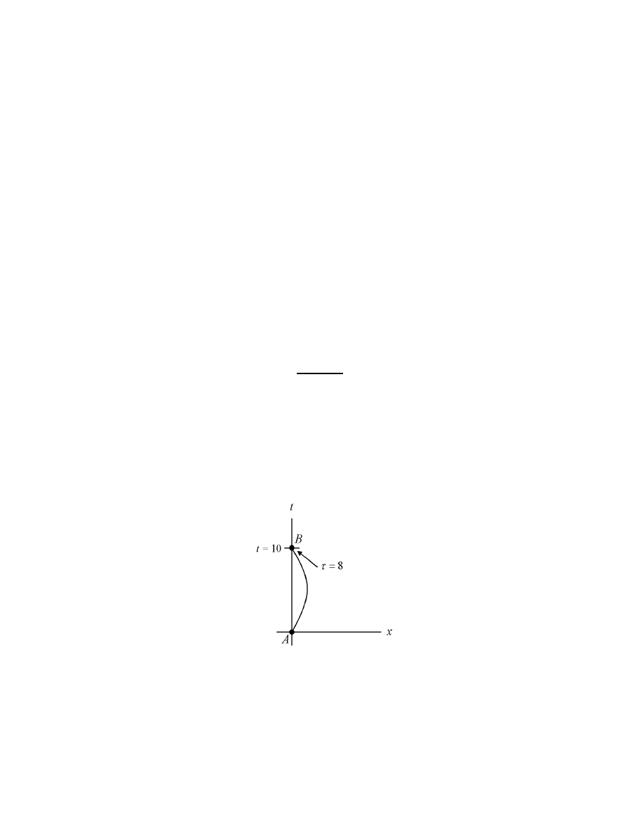
2.10 The Twin Paradox
Note. Suppose A and B are two events in spacetime separated by a
timelike interval (whose y and z coordinates are the same). Joining
these events with a straight line produces the world-line of an inertial
observer present at both events. Such an observer could view both
events as occuring at the same place (say at x = 0) and could put these
two events along his t−axis.
Note. Oddly enough, in a spacetime diagram under Lorentz geom-
etry, a straight line gives the longest distance (temporally) between
two points. This can be seen by considering the fact that the interval
(∆τ )
2
= (∆t)
2
− (∆x)
2
is invariant. Therefore, if we follow a trajectory
in spacetime that increases ∆x, it MUST increase ∆t. Figure II-19b
illustrates this fact:
That is, the non-inertial traveler (the one undergoing accelerations and
therefore the one not covered by special relativity) from A to B ages
less than the inertial traveler between these two events.
1

Example (Jack and Jill). We quote from page 152 of the text: “Let
us imagine that Jack is the occupant of a laboratory floating freely in
intergalactic space. He can be considered at the origin of an inertial
frame of reference. His twin sister, Jill, fires the engines in her rocket,
initially alongside Jack’s space laboratory. Jill’s rocket is accelerated
to a speed of 0.8 relative to Jack and then travels at that speed for
three years of Jill’s time. At the end of that time, Jill fires powerful
reversing engines that turn her rocket around and head it back toward
Jack’s laboratory at the same speed, 0.8. After another three-year
period, Jill returns to Jack and slows to a halt beside her brother.
Jill is then six years older. We can simplify the analysis by assuming
that the three periods of acceleration are so brief as to be negligible.
The error introduced is not important, since by making Jill’s journey
sufficiently long and far, without changing the acceleration intervals,
we could make the fraction of time spent in acceleration as small as
we wish. Assume Jill travels along Jack’s x−axis. In Figure II-20(see
below), Jill’s world-line is represented on Jack’s spacetime diagram. It
consists of two straight line segments inclined to the t−axis with slopes
+0.8 and −0.8, respectively. For convenience, we are using units of
years for time and light-years for distance.”
Note. Because of the change in direction (necessary to bring Jack and
Jill back together), no single inertial frame exists in which Jill is at rest.
But her trip can be described in two different inertial frames. Take the
first to have t
axis x = βt = 0.8t (in Jack’s frame). Then at t = 5 and
t
= 3, Jill turns and travels along a new t
axis of x = −0.8t + 10(in
2
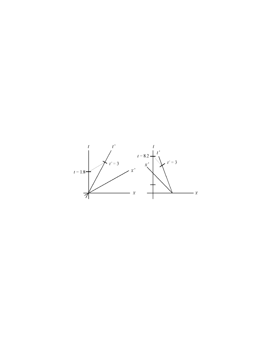
Jack’s frame). We see that upon the return, Jack has aged 10years,
but Jill has only aged 6 years. This is an example of the twin paradox.
Note. One might expect that the Principle of Relativity would imply
that Jack should also have aged less than Jill (an obvious contradiction).
However, due to the asymmetry of the situation (the fact that Jack is
inertial and Jill is not) the Principle of Relativity does not apply.
Note. Consider the lines of simultaneity for Jill at the “turning point”:
So our assumption that the effect of Jill’s acceleration is inconsequential
is suspect! Jill’s “turning” masks a long period of time in Jacks’s frame
(t = 1.8 to t = 8.2).
Note. Now suppose that Jill emits a flash of light at the end of each
3
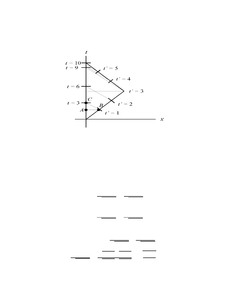
(in her frame) year. Consider the spacetime diagram:
The flash of light emitted at event B travels along a 45
◦
line (recall the
units) until it intersects the t−axis at point C and at time t
C
. Now
distance AC equals distance AB (since CBA is a 45-45-90). So
t
C
= t
A
+ AC = t
A
+ AB = t
B
+ x
B
.
With t
B
= 1 and x
B
= 0, equation (89), page 131, we have
t
B
=
βx
+ t
√
1 − β
2
=
1
√
1 − β
2
and
x
B
=
x
+ βt
√
1 − β
2
=
β
√
1 − β
2
.
We therefore have
t
C
= t
B
+ x
B
=
1
√
1 − β
2
+
β
√
1 − β
2
1 + β
√
1 − β
2
=
√
1 + β
√
1 + β
√
1 − β
√
1 + β
=
1 + β
1 − β
.
4
With β = 0.8 we have t
C
= 3. Similarly, the second flash is observed
by Jack at t = 6, and the third flash is observed at t = 9. Now the
above argument is general and we can show that if a light signal is
emitted by Jill every T units of time (in her frame), then Jack receives
the signals every
1 + β
1 − β
T units of time (in his frame). This change
in frequency is called the Doppler effect and results in a redshift (that
is, lengthening of wavelength) for β > 0and a blueshift (that is, a
shortening of wavelength) for β < 0. Notice that the flashes Jill emits
at t
= 3, t
= 4 and t
= 5 are observed by Jack at t = 9, t = 9
1
3
, and
t = 9
2
3
, respectively.
5
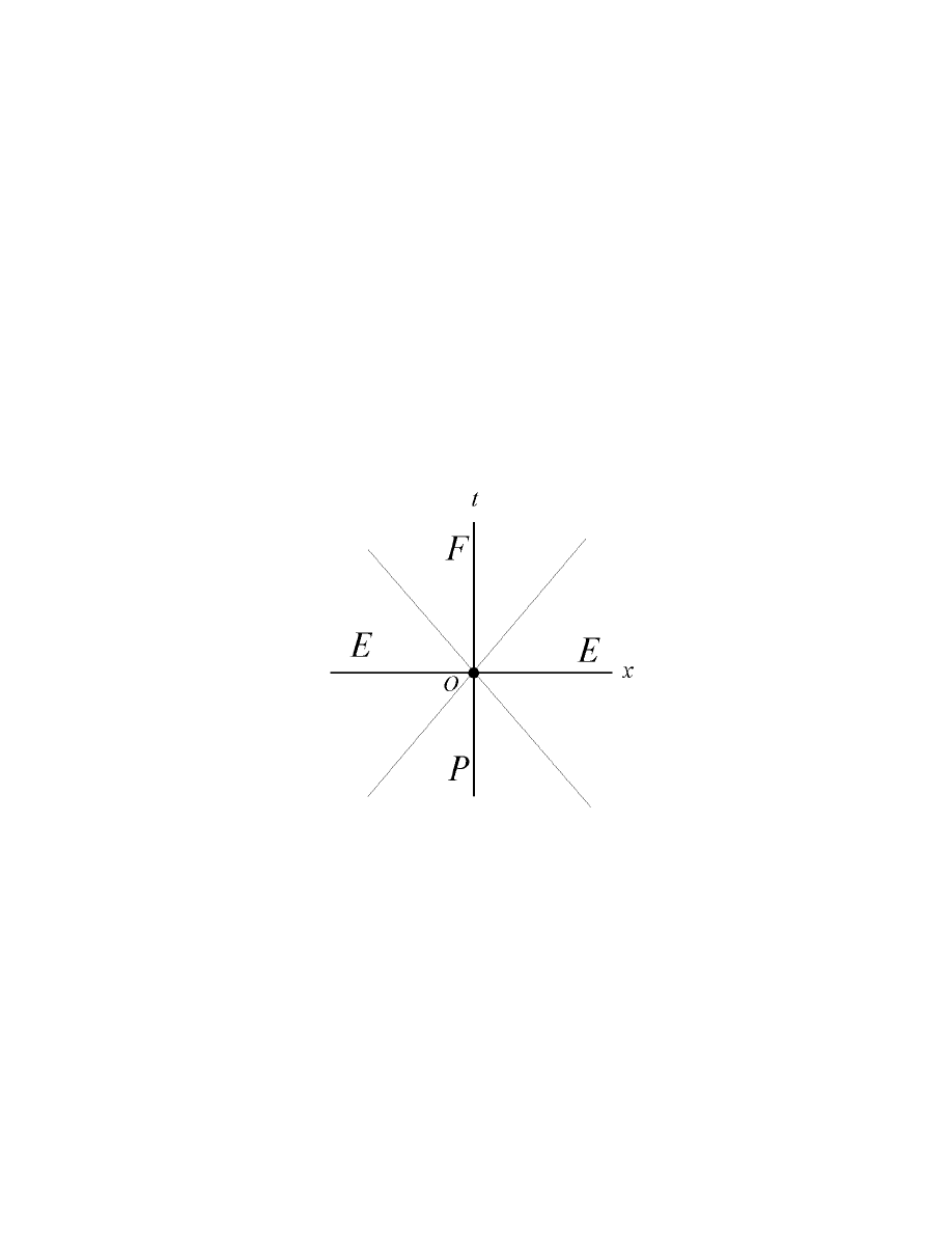
2.11 Temporal Order and Causality
Note. Suppose a flash of light is emitted at the origin of a spacetime
diagram. The wavefront is determined by the lines x = t and x = −t
where t > 0 (we use geometric units). We label the region in the upper
half plane that is between these two lines as region F . Extending
the lines into the lower half plane we similarly define region P . The
remaining two regions we label E.
Note. Events in F are separated from O by a timelike interval. So
O could influence events in F and we say O is causally connected to
the events in F . In fact, if A is an event in the interior of F , then
there is an inertial frame S
in which O and A occur at the same place.
The separation between O and A is then only one of time (and as we
claimed, O and A are separated by a timelike interval). The point A
will lie in the “future” relative to O, regardless of the inertial frame.
1

Therefore, region F is the absolute future relative to O.
Note. Similarly, events in P can physically influence O and events
in P are causally connected to O. The region P is the absolute past
relative to O.
Note. Events in region E are separated from O by a spacelike interval.
For each event C in region E, there is an inertial frame S
in which C
and O are separated only in space (and are simultaneous in time). This
means that the terms “before” and “after” have no set meaning between
O and an event in E. The region E is called elsewhere.
Note. We can extend these ideas and represent two physical dimen-
sions and one time dimension. We then find the absolute future relative
to an event to be a cone (called the future light cone). The past light
cone is similarly defined. We can imagine a 4-dimensional version where
the absolute future relative to an event is a sphere expanding in time.
2

Chapter 3. General Relativity:
The Geometry of Curved
Spacetime
Note. As we have seen, the Special Theory of Relativity deals only
with inertial (unaccelerated) observers. Such observers cannot be under
the influence of a gravitational field, and one might say that special
relativity describes the mechanics in a massless universe!
Note. In order to deal with accelerating frames of reference or frames of
reference under the influence of gravity, the Special Theory of relativity
has to be extended. This was accomplished by Einstein in his “Die
Grundlage der allgemeinen Relativit¨atstheorie” (“The Foundation of
the General Theory of Relativity”) in Annelan der Physik (Annals of
Physics) 49, 1916. As we will see, this was accomplished by considering
gravity not as a force, but as a curvature of spacetime. Falling objects,
planets in orbits, and rays of light then are observed to follow geodesics
in curved spacetime. (Surprisingly, the picture on the cover of the text
is a “straight” geodesic in a curved spacetime!)
Note. After some introductory material, we will discuss geodesics in
the semi-Riemannian 4-manifold of spacetime (Section 6) and “outline”
the reasoning which lead Einstein to his field equations (Section 7). We
will then solve the field outside an isolated sphere of mass M. Finally
(as time permits), we’ll explore orbits and the “bending of light” under
the General Theory of Relativity.
1

3.1 The Principle of Equivalence
Note. Newton’s Second Law of Motion (
F = ma) treats “mass” as
an object’s resistance to changes in movement (or acceleration). This
is an object’s inertial mass. In Newton’s Law of Universal Gravitation
(F = GMm/r
2
), an object’s mass measures its response to gravitational
attraction (called its gravitational mass). Einstein was bothered by the
dichotomy in the idea of mass:
inertial mass
acceleration
gravitational mass
gravitational acceleration
As we’ll see, he resolved this by putting gravity and acceleration on an
equivalent footing.
Note. Consider an observer in a sealed box. First, if this box is in
free fall in a gravitational field, then the observer in the box will think
that he is weightless in an inertial (unaccelerating) frame. There is no
experiment he can perform (entirely within the box) to detect the accel-
eration or the presence of the gravitational field. Second, if the observer
is out in deep space and under no gravitational influence BUT is accel-
erating rapidly, then he will interpret the acceleration as the presence
of a gravitational field. Again, there is no experiment he can perform
(within the box) which will reveal that he is accelerating rapidly, versus
being stationary with respect to a gravitational field. Einstein resolved
these observations (and the inertial versus gravitational mass question)
in the Principle of Equivalence.
1
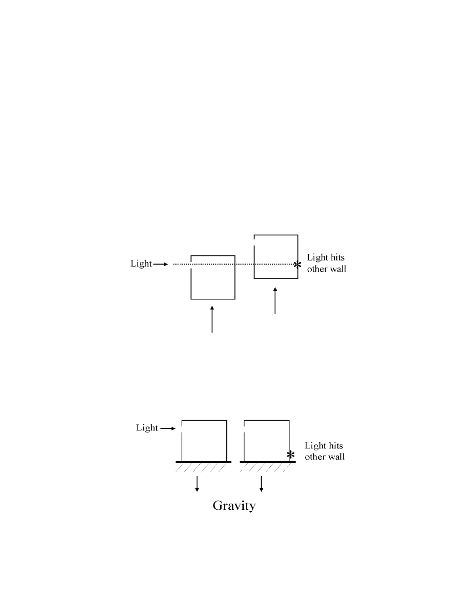
Definition. Principle of Equivalence.
There is no way to distinguish between the effects of acceleration and
the effects of gravity - they are equivalent.
Note. A consequence of the Principle of Equivalence is that light
is “bent” when in a gravitational field. Consider the observer in an
accelerating box. If a ray of light enters a hole in one side of the box,
it hits the other side of the box at a point slightly lower:
Now consider an observer in a box under the influence of gravity. By
the Principle of Equivalence, he must observe the same thing:
2
Example. Consider a collection of n particles of masses m
1
, m
2
, . . . , m
n
which interact (gravitationally, say) with force
F
ij
between particle i
and j (and so
F
ij
= −
F
ji
) for i = j. Suppose observer #1 uses co-
ordinates x, y, z, t and observer #2 uses coordinates x
, y
, z
, t
. We
assume low relative velocities and so t = t
. Let
X
i
be the location of
particle i in observer #1’s coordinates and let
X
i
be the location of
particle i in observer #2’s coordinates. We assume low relative veloci-
ties and therefore ignore relativistic effects and have t = t
. Therefore
we use
X = (x, y, z) and
X
= (x
, y
, z
) for the spatial coordinate vec-
tors. Suppose observer #1 believes that he and the particles are in the
presence of a gravitational field g (and interpretes that he is stationary
experiencing the gravity and the particles are in free fall) and so he sees
all particles moving away from him with acceleration g. The equations
of motion for the particles for observer #1 are
m
i
d
2
X
i
dt
2
= m
i
g +
j=i
F
ji
for i = 1, 2, . . . , n.
Next, Suppose observer #2 is moving relative to observer #1 in such
a way that
X
=
X −
1
2
gt
2
(Frame #2 is accelerating relative to Frame
#1 and conversely). By differentiating twice with respect to t:
d
2
X
dt
2
=
d
2
X
dt
2
− g
or
d
2
X
dt
2
=
d
2
X
dt
2
+ g.
Therefore, for the ith particle
d
2
X
i
dt
2
=
d
2
X
i
dt
2
+ g.
3

Substituting into the above equation gives
m
i
d
2
X
i
dt
2
=
j=i
F
ji
.
Therefore, the gravitational field has been “transformed” away!
• Observer #1 thinks that observer #2 (along with the particles)
is in free fall and that is why he does not “see” the gravitational
field.
• Observer #2 thinks there is no gravitational field. He thinks that
he is an inertial observer and that observer #1 is accelerating away
from observer #2 and the particles.
The Principle of Equivalence states that both observers are “right.”
Therefore the Principle of Equivalence puts all frames (inertial or not)
on the “same footing.” In particular, gravitational force is equivalent
to a force created by acceleration.
4

3.2 Gravity as Spacetime Curvature
Note. Thus far we have only considered uniform gravitational fields.
In nature, gravitational “force” varies from point to point and so the
acceleration due to this force is not uniform. First consider two parti-
cles “side by side” in a gravitational field (see Figure III-1, page 172)
directed towards a point (or the center of a sphere). As the particles
fall, they will be drawn closer together. Second, consider two particles
in a gravitational field which are separated vertically. This time, the
difference in the forces produces a growing separation between the par-
ticles as they fall. In both cases, the behavior is an example of tidal
effects. Therefore, a freely falling “space capsule” does not behave ex-
actly like an inertial frame. However, over short spans of time it is a
good approximation of an inertial frame.
Note. We rephrase the Principle of Equivalence as:
For each spacetime point (i.e. event), and for a given degree
of accuracy, there exists a frame of reference in which in a
certain region of space and for a certain interval of time,
the effects of gravity are negligible and the frame is inertial
to the degree of accuracy specified.
Such a frame is called a locally inertial frame (at the given event) and
an observer in such a frame is a locally inertial observer.
Note. The convergence and divergence of particles as described above
has a geometric analog. On a positively curved surface, “parallel” geo-
1

desics converge, and on a negatively curved surface, “parallel” geodesics
diverge (see page 175).
Note. Einstein proposed that gravity is not a force, but a curvature
of spacetime! He hypothesized that free particles (and photons) follow
geodesics in a curved spacetime.
Definition. Define the matrix of the Lorentz metric as
(η
ij
) =
1
0
0
0
0 -1
0
0
0
0 -1
0
0
0
0 -1
.
Note. A locally inertial observer in a locally inertial frame can set up
a system of coordinates where the interval satisfies
dτ
2
≈ η
ij
du
i
du
j
= (du
0
)
2
− (du
1
)
2
− (du
2
)
2
− (du
3
)
2
.
More precisely, a coordinate system (u
i
) can be set up at a point
P in
a locally inertial frame such that
dτ
2
= g
ij
du
i
du
j
and the functions g
ij
satisfy
g
ij
(
P ) = η
ij
∂g
ij
∂u
k
P
= 0.
These two conditions imply that the metric is the Lorentz metric at
P ,
and that the metric differs little from the Lorentz metric near
P (i.e.
the rate of change of the g
ij
’s is small near
P ).
2
Definition. A coordinate system such that dτ
2
= g
ij
du
i
du
j
where g
ij
are functions of u
i
(i = 0, 1, 2, 3) satisfying
g
ij
(
P ) = η
ij
∂g
ij
∂u
k
= 0
for i, j, k = 0, 1, 2, 3, at some point
P is a locally Lorentz coordinate
system at
P .
Note. We are again back to the idea of a manifold. The Principle of
Equivalence tells us that in the 4-manifold of general relativity, small
local neighborhoods look like the “flat” 4-manifold of special relativity.
The departure (on a larger scale) of dτ
2
from the Lorentz metric is due
to the nonuniformity of gravity and is the result (as we will see) of the
curvature of spacetime!
3
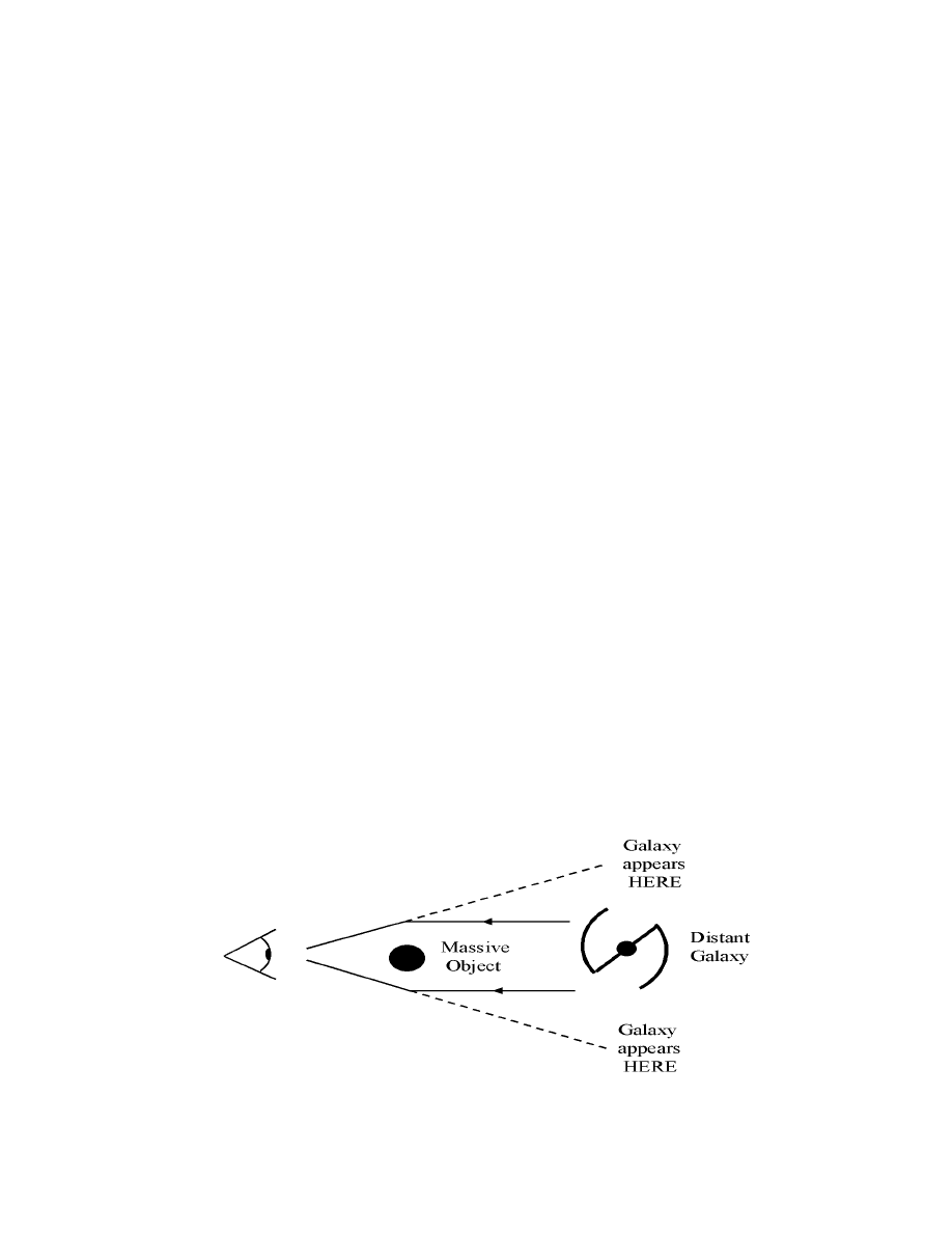
3.3 The Consequences of Einstein’s Theory
Note. Since we postulate that gravity is a curvature of spacetime
and that photons follow geodesics in spacetime, we find that “gravity
bends light” (precisely, its the spacetime which is bent). The effect
was experimentally verified in the famous 1919 eclipse expedition of
Arthur Eddington. During a total eclipse of the Sun, the position of a
star very near the Sun’s limb was measured. The star’s position was
found to be shifted by an amount predicted by the general theory. See
Figure III-4 on page 183. This experiment played a big role in making
Einstein the “science genius” and public figure that he was to become
in the 20’s, 30’s and 40’s. This experiment has been reproduced a
number of times using radio sources. A more contemporary example
which is also a consequence of this “bending of light” is gravitational
lensing. If a very distant galaxy is precisely along our line of site with
a massive foreground object, then we will see multiple images of the
background galaxy as the foreground object “focuses” the light rays.
In some situations, the image appears curved and is a segment of the
so called Einstein ring.
1

Note. A second example of experimental evidence for the general the-
ory is the precession of the orbit of Mercury. Mercury orbits the Sun
in an elliptical orbit (e ≈ .2) and therefore experiences different accel-
erations due to the Sun. This results in a precession (or shifting) of
the perihelion (point of the orbit furthest from the Sun) over consec-
utive orbits (see Figure III-5, page 185). The observed precession is
43.11 ± 0.45
per century and general relativity predicts a precession of
43.03
per century (see Section 3.9 and Table III-2, page 230).
Note. Another prediction is the gravitational redshift of a photon in a
strong gravitational field. We’ll explore this in Sections 3.7 and 3.8.
2
3.6 Geodesics
Note. We now view spacetime as a semi-Riemannian 4-manifold such
that for each coordinate system (x
0
, x
1
, x
2
, x
3
)
(dτ )
2
= g
µν
dx
µ
dx
ν
where the g
µν
are functions of the coordinates.
Definition. A vector v = v
µ
∂
∂x
µ
is timelike, lightlike, or spacelike if
v,v = g
µν
v
µ
v
ν
is positive, zero, or negative, respectively.
Definition. A spacetime curve α is a geodesic if it has a parameteri-
zation x
λ
(ρ) satisfying
d
2
x
λ
dρ
2
+ Γ
λ
µν
dx
µ
dρ
dx
ν
dρ
= 0
(120)
for λ = 0, 1, 2, 3.
Note. “It can be shown” that the definition of geodesic is independent
of a choice of coordinate system (says the text, page 198).
Note. If α is a geodesic, then
α
, α
=
dτ
dρ
2
= g
µν
dx
µ
dρ
dx
ν
dρ
is constant (with the same proof as given at the bottom of page 68).
Definition. A geodesic α is timelike, lightlike, or spacelike according
to whether α
, α
is positive, zero, or negative.
1

Note. If a geodesic α is timelike, then dτ /dρ = constant, and we have
ρ = aτ +b for some a and b. We then see that equation (120) still holds
when we replace ρ with τ .
Note. If a geodesic α is lightlike then
α
, α
=
dτ
dρ
2
= 0
and τ is constant along α. Therefore proper time τ cannot be used to
reparameterize α.
Note. If a geodesic α is spacelike, then dτ /dρ is imaginary. The proper
distance
dσ =
(dx)
2
+ (dy)
2
+ (dz)
2
− (dt)
2
= idτ
can be used to parameterize α. We have dσ/dρ a real constant and so
ρ = aσ + b for some a and b. We see that equation (120) still holds
when we replace ρ with σ.
Definition. A curve α is timelike if α
, α
> 0 at each of its points.
Theorem III-2. Let α be a timelike curve which extremizes spacetime
distance (i.e. the quantity ∆τ ) between its two end points. Then α is
a geodesic.
Idea of the proof. The curve can be parameterized in terms of τ (as
remarked above). The proof then follows as did the proof of Theorem
I-9.
2

Theorem III-3. Given an event
P and a nonzero vector v at P , then
there exists a unique geodesic α such that α(0) =
P and α
(0) = v.
Note. Theorem III-3 implies that all particles in a gravitational field
will fall with the same acceleration dependent only on initial position
and velocity. That is, we don’t see heavier objects fall faster!
Note. In the absence of gravity, a particle follows a path
d
2
x
λ
dρ
2
= 0 (that
is, the particle follows a straight line!). We can therefore interprete the
Christoffel symbols as the components of the gravitational field.
3
3.7 The Field Equations
Note. We now want a set of equations relating the metric coefficients
g
µν
which determine the curvature of spacetime due to the distribution
of matter in spacetime. Einstein accomplished this in his “Die Grund-
lage der allgemeinen Relativit¨atstheorie”(The Foundation of the Gen-
eral Theory of Relativity) in Annalen der Physik (Annals of Physics)
in 1916.
Note. Consider a mass M at the origin of a 3-dimensional system. Let
X = (x, y, z) = (x(t), y(t), z(t)), and
X =
√
x
2
+ y
2
+ z
2
= r. Let u
r
be the unit radial vector
X/r. Under Newton’s laws, the force F on a
particle of mass m located at
X is
F = −Mm
r
2
u
r
= m
d
2
X
dt
2
.
Therefore
d
2
X
dt
2
= −
M
r
2
u
r
.
Definition. For a particle at point (x, y, z) in a coordinate system
with mass M at the origin, define the potential function Φ = Φ(r) as
Φ(r) = −
M
r
where r =
√
x
2
+ y
2
+ z
2
.
Theorem. The potential function satisfies Laplace’s equation
∇
2
Φ =
∂
2
Φ
∂x
2
+
∂
2
Φ
∂y
2
+
∂
2
Φ
∂z
2
= 0
1

at all points except the origin.
Proof. First
∂r
∂x
i
=
∂
∂x
i
[(
X ·
X)
1/2
] =
2x
i
2(
X ·
X)
1/2
=
x
i
r
and
∂Φ
∂x
i
=
∂Φ
∂r
∂r
∂x
i
.
Therefore
−∇Φ = −
∂Φ
∂x
,
∂Φ
∂y
,
∂Φ
∂z
= −
M
r
2
x
r
,
y
r
,
z
r
= −
M
r
2
u
r
=
d
2
X
dt
2
.
Comparing components,
d
2
x
i
dt
2
= −
∂Φ
∂x
i
.
(122)
Differentiating the relationship
∂Φ
∂x
i
=
∂
∂x
i
−
M
r
=
∂
∂x
i
−M
((x
1
)
2
+ (x
2
)
2
+ (x
3
)
2
)
1/2
=
−1(−1/2)M(2x
i
)
((x
1
)
2
+ (x
2
)
2
+ (x
3
)
2
)
3/2
=
Mx
i
r
3
gives
∂
2
Φ
(∂x
i
)
2
= M
r
3
− x
i
[(3/2)r(2x
i
)]
r
6
= M
r
3
− 3r(x
i
)
2
r
6
=
M
r
5
(r
2
− 3(x
i
)
2
).
2
Summing over i = 1, 2, 3 gives
∇
2
Φ =
M
r
5
{(r
2
− 3(x
1
)
2
) + (r
2
− 3(x
2
)
2
) + (r
2
− 3(x
3
)
2
)} = 0.
Note. In the case of a finite number of point masses, the Laplace’s
equation still holds, only Φ is now a sum of terms (one for each particle).
Note. In general relativity, we replace equation (122) with
d
2
x
λ
dτ
2
+ Γ
λ
µν
dx
µ
dτ
dx
ν
dτ
= 0
(125)
where the Christoffel symbols are
Γ
λ
µν
=
1
2
g
λβ
∂g
µβ
∂x
ν
+
∂g
νβ
∂x
µ
−
∂g
µν
∂x
β
.
Note. Comparing equations (122) and (125), we see that
∂Φ
∂x
i
and Γ
λ
µν
dx
µ
dτ
dx
ν
dτ
play similar roles. As the text says, “in a sense then, the metric coef-
ficients play the role of gravitational potential functions in Einstein’s
theory.”
Note. Trying to come up with a result analogous to Laplace’s equation
and treating the g
µν
’s as a potential function, we might desire a field
equation of the form G = 0 where G involves the second partials of the
g
µν
’s.
3

Note. “It turns out”that the only tensors that are constructible from
the metric coefficients g
µν
and their first and second derivatives are
those that are functions of g
µν
and the components of R
λ
µνσ
of the
curvature tensor.
Note. We want the field equations to have the flat spacetime of special
relativity as a special case. In this special case, the g
µν
are constants
and so we desire R
λ
µνσ
= 0 for each index ranging from 0 to 3 (since the
partial derivatives of the g
µν
are involved). However, “it can be shown”
that this system of PDEs (in the unknown g
µν
’s) implies that the g
µν
’s
are constant (and therefore that we are under the flat spacetime of
special relativity... we could use some details to verify this!).
Definition. The Ricci tensor is obtained from the curvature tensor by
summing over one index:
R
µν
= R
λ
µνλ
=
∂Γ
λ
µλ
∂x
ν
−
∂Γ
λ
µν
∂x
λ
+ Γ
β
µλ
Γ
λ
νβ
− Γ
β
µν
Γ
λ
βλ
.
Note. Einstein chose as his field equations the system of second order
PDEs R
µν
= 0 for µ, ν = 0, 1, 2, 3. More explicitly:
Definition. Einstein’s field equations for general relativity are the
system of second order PDEs
R
µν
=
∂Γ
λ
µλ
∂x
ν
−
∂Γ
λ
µν
∂x
λ
+ Γ
β
µλ
Γ
λ
νβ
− Γ
β
µν
Γ
λ
βλ
= 0
where
Γ
λ
µν
=
1
2
g
λβ
∂g
µβ
∂x
ν
+
∂g
νβ
∂x
µ
−
∂g
µν
∂x
β
.
4

Therefore, the field equations are a system of second order PDEs in the
unknown function g
µν
(16 equations in 16 unknown functions). The g
µν
determine the metric form of spacetime and therefore all intrinsic prop-
erties of the 4-dimensional semi-Riemannian manifold that is spacetime
(such as curvature)!
Note. The text argues that in a weak static gravitational field, we
need
g
00
= 1 + 2Φ.
(135)
See pages 204-206 for the argument. We will need this result in the
Schwarzschild solution of the next section.
Lemma III-4. For each µ,
g
λβ
∂g
λβ
∂x
µ
=
1
g
∂g
∂x
µ
=
∂
∂x
µ
[ln |g|].
Proof. See pages 207-208. We will use this result in the derivation of
the Schwarzschild solution.
5

3.8 The Schwarzschild Solution
Note. In this section, we solve Einstein’s field equations for the grav-
itational field outside an isolated sphere of mass M assumed to be at
rest at the (spatial) origin of our coordinate system.
Note. We convert to spherical coordinates ρ, φ, θ:
x = ρ sin φ cos θ
y = ρ sin φ sin θ
z = ρ cos φ.
In the event of flat spacetime, we have the Lorentz metric
dτ
2
= dt
2
− dx
2
− dy
2
− dz
2
= dt
2
− dρ
2
− ρ
2
dφ
2
− ρ
2
sin
2
φ dθ
2
.
(144)
Note. As the book says, “the derivation that follows is not entirely
rigorous, but it does not have to be - as long as the resulting metric
form is a solution to the field equations.”
Note. We have a static gravitational field (i.e. independent of time)
and it is spherically symmetric (i.e. independent of φ and θ) so we look
for a metric form satisfying
dτ
2
= U(ρ)dt
2
− V (ρ)dρ
2
− W (ρ)(ρ
2
dφ
2
+ ρ
2
sin
2
φ dθ
2
)
(145)
where U, V, W are functions of ρ only. Let r = ρ
W (ρ) then (145)
1

becomes
dτ
2
= A(r)dt
2
− B(r)dr
2
− r
2
dφ
2
− r
2
sin
2
φ dθ
2
(146)
for some A(r) and B(r). Next define functions m = m(r) and n = n(r)
where
A(r) = e
2m(r)
= e
2m
and B(r) = e
2n(r)
= e
2n
.
Then (146) becomes
dτ
2
= e
2m
dt
2
− e
2n
dr
2
− r
2
dφ
2
− r
2
sin
2
φ dθ
2
.
(147)
Since dτ
2
= g
µν
dx
µ
dx
ν
in general, if we label x
0
= t, x
1
= r, x
2
= φ,
x
3
= θ we have
(g
µν
) =
e
2m
0
0
0
0
−e
2n
0
0
0
0
−r
2
0
0
0
0
−r
2
sin
2
φ
and g = det(g
ij
) = −e
2m+2n
r
4
sin
2
φ. If we find m(r) and n(r), we will
have a solution!
Note. We need the Christoffel symbols
Γ
λ
µν
=
1
2
g
λβ
∂g
µβ
∂x
ν
+
∂g
νβ
∂x
µ
−
∂g
µν
∂x
β
.
(126)
Since g
µν
= 0 for µ = ν, we have g
µµ
= 1/g
µµ
and g
µν
= 0 if µ = ν. So
the coefficient g
λβ
is 0 unless β = λ and we have
Γ
λ
µν
=
1
2g
λλ
∂g
µλ
∂x
ν
+
∂g
νλ
∂x
µ
−
∂g
µν
∂x
λ
.
We need to consider three cases:
2

Case 1. For λ = ν:
Γ
ν
µν
=
1
2g
νν
∂g
µν
∂x
ν
+
∂g
νν
∂x
µ
−
∂g
µν
∂x
ν
=
1
2g
νν
∂g
νν
∂x
µ
=
1
2
∂
∂x
µ
[ln(g
νν
)]
Case 2. For µ = ν = λ:
Γ
λ
µµ
=
1
2g
λλ
∂g
µλ
∂x
µ
+
∂g
µλ
∂x
µ
−
∂g
µµ
∂x
λ
=
−1
2g
λλ
∂g
µµ
∂x
λ
since g
µλ
= 0 in this case.
Case 3. For µ, ν, λ distinct: Γ
λ
µν
= 0 since g
µλ
= g
νλ
= g
µν
= 0 in this
case.
Note. With the g
µν
’s given above (in terms of m, n, r and φ) we can
calculate the nonzero Christoffel symbols to be:
Γ
0
10
= Γ
0
01
= m
Γ
1
00
= m
e
2m−2n
Γ
1
11
= n
Γ
1
22
= −re
−2n
Γ
2
12
= Γ
2
21
=
1
r
Γ
1
33
= −re
−2n
sin
2
φ
Γ
3
13
= Γ
3
31
=
1
r
Γ
3
23
= Γ
3
32
= cot φ
Γ
2
33
= − sin φ cos φ
where = d/dr.
Note. W e have
ln |g|
1/2
=
1
2
ln(e
2m+2n
r
4
sin
2
φ) = m + n + 2 ln r + ln(sin φ).
3
We saw in Lemma III-4 that
g
λβ
∂g
λβ
∂x
µ
=
1
g
∂g
∂x
µ
=
∂
∂x
µ
[ln |g|].
Now
∂
∂x
β
[ln |g|
1/2
] =
1
2
∂
∂x
β
[ln |g|] =
1
2
g
λµ
∂g
λµ
∂x
β
=
1
2
g
λλ
∂g
λλ
∂x
β
.
Also, from (126)
Γ
λ
µν
=
1
2
g
λβ
∂g
µβ
∂x
ν
+
∂g
νβ
∂x
µ
−
∂g
µν
∂x
β
we have with µ = β, ν = λ and δ the dummy variable:
Γ
λ
βλ
=
1
2
g
λδ
∂g
βδ
∂x
λ
+
∂g
λδ
∂x
β
−
∂g
βλ
∂x
δ
=
1
2
g
λλ
∂g
βλ
∂x
λ
+
∂g
λλ
∂x
β
−
∂g
βλ
∂x
λ
=
1
2
g
λλ
∂g
λλ
∂x
β
.
Therefore we have
∂
∂x
β
[ln |g|
1/2
] = Γ
λ
βλ
.
Similarly
∂
∂x
µ
[ln |g|
1/2
] = Γ
λ
µλ
. Therefore the field equations imply
R
µν
=
∂
2
∂x
µ
∂x
ν
[ln |g|
1/2
] −
∂Γ
λ
µν
∂x
λ
+ Γ
β
µλ
Γ
λ
νβ
− Γ
β
µν
∂
∂x
β
[ln |g|
1/2
] = 0.
Note. We find that
R
00
=
−m
+ m
n
− m
2
−
2m
r
e
2m−2n
R
11
= m
− m
n
+ m
2
−
2n
r
R
22
= e
−2n
(1 + rm
− rn
) − 1
R
33
= R
22
sin
2
φ
4
All other R
µν
are identically zero. Next, the field equations say that
we need each of these to be zero. Therefore we need:
−m
+ m
n
− m
2
−
2m
r
= 0
m
− m
n
+ m
2
−
2n
r
= 0
e
−2n
(1 + rm
− rn
) − 1 = 0
R
22
sin
2
φ = 0
Adding the first two of these equations, we find that m
+n
= 0, and so
m + n = b, a constant. However, by the boundary conditions both
m and n must vanish as r → ∞, since the metric (147) must approach
the Lorentz metric at great distances from the mass M (compare (147)
and (144)). Therefore, b = 0 and n = −m. The third equation implies:
1 = (1 + 2rm
)e
2m
= (re
2m
)
.
Hence we have re
2m
= r + C for some constant C, or g
00
= e
2m
= 1 +
C/r. But as commented in the previous section, we need g
00
= 1−2M/r
where the field is weak. We therefore have C = −2M. Therefore we
have the solution:
dτ
2
=
1 −
2M
r
dt
2
−
1 −
2M
r
−1
dr
2
− r
2
dφ
2
− r
2
sin
2
φ dθ
2
.
Note. This solution was derived a few months after Einstein published
his paper in 1916. Notice that we have r = ρ and W (ρ) = 1.
5
3.9 Orbits in General Relativity
Note. We now calculate the geodesic which describes the orbit of
an object about another object of mass M located at the (spatial)
origin. This means that we desire to describe a geodesic under the
“Schwarzschild metric” of the previous section.
Note. We start with the Schwarzschild metric
dτ
2
=
1 −
2M
r
dt
2
−
1 −
2M
r
−1
dr
2
− r
2
dφ
2
− r
2
sin
2
φ dθ
2
and describe the path of a planet by a timelike geodesic
(x
0
(τ ), x
1
(τ ), x
2
(τ ), x
3
(τ ))
where
d
2
x
λ
dτ
2
+ Γ
λ
µν
dx
µ
dτ
dx
ν
dτ
= 0
for λ = 0, 1, 2, 3. As in the previous section, we take x
0
= t, x
1
= r,
x
2
= φ, and x
3
= θ. The resulting Christoffel symbols are given in
equation (153), page 214.
Note. With λ = 2 we have from the geodesic condition
d
2
x
2
dτ
2
+ Γ
2
µν
dx
µ
dτ
dx
ν
dτ
= 0
and since the only nonzero Γ’s with a superscript of 2 are Γ
2
12
, Γ
2
21
, and
Γ
2
33
we have
d
2
x
2
dτ
2
+ Γ
2
12
dx
1
dτ
dx
2
dτ
+ Γ
2
21
dx
2
dτ
dx
1
dτ
+ Γ
2
33
dx
3
dτ
dx
3
dτ
= 0
1
or
d
2
φ
dτ
2
+ 2
1
r
dr
dτ
dφ
dτ
+ (− sin φ cos φ)
dθ
dτ
2
= 0.
We orient our axes such that when τ = 0, we have φ = π/2 and
dφ/dτ = 0. So the planet starts in the plane φ = π/2 and due to
symmetry remains in this plane. So we henceforth take φ = π/2. Now
with λ = 0:
d
2
x
0
dτ
2
+ Γ
0
µν
dx
µ
dτ
dx
ν
dτ
= 0
and since the only nonzero Γ’s with a superscript of 0 are Γ
0
10
and Γ
0
01
,
we have
d
2
x
0
dτ
2
+ Γ
0
10
dx
1
dτ
dx
0
dτ
+ Γ
0
01
dx
0
dτ
dx
1
dτ
= 0
or
d
2
t
dτ
2
+ 2
m
dr
dτ
dt
dτ
= 0.
(159a)
With λ = 1 :
d
2
x
1
dτ
2
+ Γ
1
µν
dx
µ
dτ
dx
ν
dτ
= 0
and since the only nonzero Γ’s with a superscript of 1are Γ
1
00
, Γ
1
11
, Γ
1
22
,
and Γ
1
33
, we have
d
2
x
1
dτ
2
+ Γ
1
00
dx
0
dτ
dx
0
dτ
+ Γ
1
11
dx
1
dτ
dx
1
dτ
+ Γ
1
22
dx
2
dτ
dx
2
dτ
+ Γ
1
33
dx
3
dτ
dx
3
dτ
= 0
or
d
2
r
dτ
2
+ m
e
2m−2n
dt
dτ
2
+ n
dr
dτ
2
+(−re
−2n
)
dφ
dτ
2
+ (−re
−2n
sin
2
φ)
dθ
dτ
2
= 0.
(159b)
(since we have φ = π/2, sin
2
φ ≡ 1). With λ = 3
d
2
x
3
dτ
2
+ Γ
3
µν
dx
µ
dτ
dx
ν
dτ
= 0
2
and since the only nonzero Γ’s with a superscript of 3 are Γ
3
13
, Γ
3
31
, Γ
3
23
,
and Γ
3
32
, we have
d
2
x
3
dτ
2
+ Γ
3
13
dx
1
dτ
dx
3
dτ
+ Γ
3
31
dx
3
dτ
dx
1
dτ
+ Γ
3
23
dx
2
dτ
dx
3
dτ
+ Γ
3
32
dx
3
dτ
dx
2
dτ
= 0
or
d
2
θ
dτ
2
+ 2
1
r
dr
dτ
dθ
dτ
+ 2
cot φ
dφ
dτ
dθ
dτ
= 0
or since φ = π/2
d
2
θ
dτ
2
+ 2
1
r
dr
dτ
dθ
dτ
= 0.
(159c)
Note. Now by the Chain Rule m
dr
dτ
=
dm
dr
dr
dτ
=
dm
dτ
, and dividing
(159a) by dt/dτ gives
d
2
t/dτ
2
dt/dτ
+ 2
m
dr
dτ
= 0
or
d
dτ
ln
dt
dτ
= −2
dm
dτ
.
Integration yields
ln
dt
dτ
= −2m + constant
or
dt
dτ
= be
−2m
=
b
γ
(160)
where b is some positive constant and we define γ = e
2m
.
Note. Equation (159c) can be integrated (see page 63 for the process)
to yield
r
2
dθ
dτ
= h
(161)
3
where h is a positive constant.
Note. From the Schwarzschild metric with φ = π/2, dφ = 0, and
γ = e
2m
= 1 − 2M/r we have
dτ
2
= γdt
2
− γ
−1
dr
2
− r
2
dθ
2
or
1 = γ
dt
dτ
2
− γ
−1
dr
dτ
2
− r
2
dθ
dτ
2
= γ
b
γ
2
− γ
−1
dr
dθ
h
r
2
2
− r
2
h
r
2
2
(162)
by equation (160), the fact that
dr
dτ
=
dr
dθ
dθ
dτ
=
dr
dθ
h
r
2
(by the Chain Rule and equation (161)) and by equation (161). Multi-
plying (162) by γ yields
γ = b
2
−
dr
dθ
h
r
2
2
− γ
h
2
r
2
or since γ = 1 − 2M/r:
1 −
2M
r
= b
2
−
h
r
2
2
dr
dθ
2
−
1 −
2M
r
h
2
r
2
or
h
r
2
dr
dθ
2
+
h
2
r
2
= b
2
− 1 +
2M
r
+
2M
r
h
2
r
2
.
Let u = 1/r so that
du
dθ
= −
1
r
2
dr
dθ
and the previous equation yields
1
r
2
dr
dθ
2
+
1
r
2
=
b
2
− 1
h
2
+
2M
rh
2
+
2M
r
3
4
or
u
2
dr
dθ
2
+ u
2
=
b
2
− 1
h
2
+
2Mu
h
2
+ 2Mu
3
or
du
dθ
2
+ u
2
=
b
2
− 1
h
2
+
2Mu
h
2
+ 2Mu
3
.
Differentiation with respect to θ yields
2
du
dθ
d
2
u
dθ
2
+ 2u
du
dθ
=
2M
h
2
du
dθ
+ 6Mu
2
du
dθ
or
d
2
u
dθ
2
+ u =
M
h
2
+ 3Mu
2
(163)
where u = 1/r and h = r
2
dθ/dτ (constant).
Note. A similar analysis in the Newtonian setting yields
d
2
u
dθ
2
+ u =
M
h
2
(114)
(see page 193). So the only difference is the 3Mu
2
term in (163) and we
can think of this as the “relativistic term.” Equation (114) has solution
u =
M
h
2
(1+ e cos θ).
Note. We can view (163) as a linear ODE (considering the left hand
side) set equal to a nonhomogeneous term
M
h
2
+ 3Mu
2
. Now the term
3Mu
2
is “small” as compared to M/h
2
(see page 226). We perturb this
equation by replacing u with the approximate solution M/h
2
(1+e cos θ)
on the right hand side of (163) and consider
d
2
u
dθ
2
+ u =
M
h
2
+ 3M
M
h
2
(1+ e cos θ)
2
5
=
M
h
2
+
3M
3
h
4
(1+ 2e cos θ + e
2
cos
2
θ).
A solution to this (linear) ODE will then be an approximate solution
to (163). The ODE is
d
2
u
dθ
2
+ u =
M
h
2
+
3M
3
h
4
+
6M
2
e
h
4
cos θ +
3M
3
e
2
2h
4
+
3M
3
e
2
2h
4
cos(2θ). (165)
(The last two terms follow from the fact that cos
2
θ = (1 + cos(2θ))/2.)
Lemma III-5. Let A ∈ R. Then
1. u = A is a solution of d
2
u/dθ
2
+ u = A.
2. u = (A/2)θ sin θ is a solution of d
2
u/dθ
2
+ u = A cos θ.
3. u = (−A/3) cos(2θ) is a solution of d
2
u/dθ
2
+ u = A cos(2θ).
(The proof follows by simply differentiating.)
Note. Equation (165) is
d
2
u
dθ
2
+ u =
M
h
2
+
3M
3
h
4
+
3M
3
e
2
2h
4
+
6M
3
e
h
4
cos θ
+
3M
3
e
2
2h
4
cos(2θ)
and by Lemma III-5
u =
M
h
2
+
3M
3
h
4
+
3M
3
e
2
2h
4
+
3M
3
e
h
4
θ sin θ
+
−M
3
e
2
2h
4
cos(2θ)
=
M
h
2
1 +
3M
2
h
2
1 +
e
2
2
+
3M
2
e
h
2
θ sin θ −
M
2
e
2
2h
2
cos(2θ)
is a (particular) solution to (165). Now the general solution to the
homogeneous ODE
d
2
u
dθ
2
+ u = 0
6
is a linear combination of u = sin θ and u = cos θ. Therefore, we can
add any linear combination of these functions to the above particular
solution to get another solution. We choose to add
M
h
2
e cos θ (for rea-
sons to be discussed shortly - we want to compare this solution to the
Newtonian solution). We have
u =
M
h
2
1 +
3M
2
h
2
1 +
e
2
2
+ e cos θ +
3M
2
e
h
2
θ sin θ −
M
2
e
2
2h
2
cos(2θ)
.
Note. The term
3M
2
h
2
1 +
e
2
2
is small compared to 1(8 × 10
−8
for
Mercury, see page 227). If we let
α = 1 +
3M
2
h
2
1 +
e
2
2
and define e
= e/α then
Mα
h
2
(1+e
cos θ) =
M
h
2
(α+e cos θ) =
M
h
2
1 +
3M
2
h
2
1 +
e
2
2
+ e cos θ
.
Since α ≈ 1, e
≈ e and we see that this part of the u function is
approximately the same as the Newtonian solution. A similar argu-
ment shows that the “cos(2θ)” term causes little deviation from the
Newtonian solution. Therefore we have that
u ≈
M
h
2
1 + e cos θ +
3M
2
e
h
2
θ sin θ
.
Although the “θ sin θ” may be very small initially, as θ increases “the
term will have a cumulative effect over many revolutions” (see page
228). This effect is the observed perihelial advance.
7
Note. Since M
2
/h
2
is small (≈ 10
−8
for Mercury, see page 228) we
approximate
cos
3M
2
θ
h
2
≈ 1,
sin
3M
2
θ
h
2
≈
3M
2
θ
h
2
and we get
M
h
2
1 + e cos
θ −
3M
2
h
2
θ
=
M
h
2
1 + e
cos θ cos
3M
2
h
2
θ
+ sin θ sin
3M
2
h
2
θ
≈
M
h
2
1 + e cos θ + e
3M
2
h
2
θ sin θ
= u.
So u has a maximum (and r = 1/u has a minimum - i.e. we are at
perihelion) when cos
θ −
3M
2
h
2
θ
is at a maximum. This occurs for
θ = 0 and
θ =
2π
1 − 3M
2
/h
2
≈ 2π
1 +
3M
2
h
2
(since (1 − x)
−1
≈ 1 + x for x ≈ 0). So the perihelion advances (in the
direction of the orbital motion) by an amount 6πM
2
/h
2
per revolution.
Note. If we want the orbital precession per century, we have
∆θcent = n∆θ =
6πM
2
n
h
2
=
6πMn
a(1 − e
2
)
(since h
2
/M
2
= a(1 − e
2
) by equation (119)) where n is the number of
orbits of the Sun that a planet makes per century.
8

Note. Table III-2 gives the calculated precessions as observed and as
predicted for 4 solar system objects. The last two columns represent
precessions measured in seconds per century:
Planet
a(÷10
11
cm)
e
n General Relativity
Observed
Mercury
57.91
0.2056 415
43.03
43.11 ± 0.45
Venus
108.21
0.0068 149
8.6
8.4 ± 4.8
Earth
149.60
0.0167 100
3.8
5.0 ± 1.2
Icarus
161.0
0.827
89
10.3
9.8 ± 0.8
9
3.10 The Bending of Light
Note. A photon of light follows a lightlike geodesic for which dτ = 0.
Such a geodesic, therefore, cannot be parameterized in terms of τ . So
we parameterize in terms of some ρ where dτ /dρ = 0. As in the previous
section, let the geodesic be (x
0
(ρ), x
1
(ρ), x
2
(ρ), x
3
(ρ)) and we have:
d
2
x
λ
dρ
2
+ Γ
λ
µν
d
µ
dρ
dx
ν
dρ
= 0
for λ = 0, 1, 2, 3.
Note. As in the previous section, we desire equations (159a-c) with τ
replaced with ρ (again, we assume the photon is restricted to the plane
φ = π/2).
Note. As in the previous section
dτ
2
=
1 −
2M
r
dt
2
−
1 −
2M
r
−1
dr
2
− r
2
dφ
2
− r
2
sin
2
φ dθ
2
(this is equation (157)) and so
dτ
2
= γdt
2
− γ
−1
dr
2
− r
2
dθ
2
(since φ = π/2 and dφ = 0) and
dτ
2
dρ
2
= γ
dt
dρ
2
− γ
−1
dr
dρ
2
− r
2
dθ
dρ
2
where γ = 1 − 2M/r. Now dτ /dρ = 0 so with the notation of the
previous section (see equation (162)) we have
0 = γ
b
γ
2
− γ
−1
dr
dθ
h
r
2
2
− r
2
h
r
2
2
1
or
0 = b
2
−
dr
dθ
h
r
2
2
− γr
2
h
r
2
2
or
h
r
2
dr
dθ
2
+ γ
h
2
r
2
= b
2
.
Now (as on page 226) with u = 1/r and
du
dθ
=
−1
r
2
dr
dθ
we get
h
2
du
dθ
2
+
1 −
2M
r
h
2
u
2
= b
2
or
du
dθ
2
+ u
2
=
b
2
h
2
+
2Mu
2
r
=
b
2
h
2
+ 2Mu
3
.
Differentiating with respect to θ implies
2
du
dθ
d
2
u
dθ
2
+ 2u
du
dθ
= 0 + 6Mu
2
du
dθ
or (dividing by 2du/dθ):
d
2
u
dθ
2
+ u = 3Mu
2
(168)
(compare to (163)).
Note. We orient our coordinate system such that the closest approach
of the geodesic occurs at θ = 0. If M = 0, the general solution to (168)
(a homogeneous equation under this condition) is u = α cos θ + β sin θ.
If we let R be the minimum distance of the geodesic from M (assumed
to occur at θ = 0) we have α = 1/R. With M = 0, geodesics are
“straight lines” and so β = 0 and u = (1/R) cos θ.
2
Note. We modify (168) by substituting u = (1/R) cos θ in the right
hand side to produce (as in the previous section)
d
2
u
dθ
2
+ u ≈ 3M
1
R
cos θ
2
=
3M
R
2
cos
2
θ
=
3M
2R
2
(1 +cos(2θ)) .
By Lemma III-5, a particular solution is
u =
3M
2R
2
1 −
1
3
cos(2θ)
or (since cos(2θ) = 2 cos
2
θ − 1)):
u =
M
R
2
(2 − cos
2
θ).
Now adding the homogeneous solution u = (1/R) cos θ to this particular
solution we get
u =
1
r
=
M
R
2
(2 − cos
2
θ) +
1
R
cos θ. (170)
Note. From Figure III-10, we have for r → ∞, θ approaches ±(π/2 +
∆θ/2). Since ∆θ ≈ 0, cos
2
θ ≈ 0 and so for r → ∞ we have from (170)
that
u =
1
r
≈ 0 ≈
1
R
cos θ +
M
R
2
(2 − cos
2
θ)
→
1
R
cos
π
2
+
∆θ
2
+
2M
R
2
− 0.
Or
2M
R
2
=
−1
R
cos
π
2
+
∆θ
2
=
1
R
sin
∆θ
2
≈
∆θ
2R
.
Therefore
∆θ
2
≈
2M
R
and ∆θ ≈
4M
R
.
3

Note. If we assume a photon undergoes a Newtonian acceleration, we
find that Newtonian mechanics implies that a photon follows a hyper-
bolic trajectory with ∆θ =
2M
R
when grazing the Sun. This is half
the displacement predicted by general relativity.
Note. As indicated previously, experiment agrees strongly with Ein-
stein’s theory! It’s relative!
4
Special Topic: Black Holes
Primary Source: A Short Course in General Relativity, 2nd Ed., J.
Foster and J.D. Nightingale, Springer-Verlag, N.Y., 1995.
Note. Suppose we have an isolated spherically symmetric mass M with
radius r
B
which is at rest at the origin of our coordinate system. Then
we have seen that the solution to the field equations in this situation is
the Schwarzschild solution:
dτ
2
=
1 −
2M
r
dt
2
−
1 −
2M
r
−1
dr
2
− r
2
dφ
2
− r
2
sin
2
φ dθ.
Notice that at r = 2M, the metric coefficient g
11
is undefined. Therefore
this solution is only valid for r > 2M. Also, the solution was derived
for points outside of the mass, and so r must be greater than the radius
of the mass r
B
. Therefore the Schwarzschild solution is only valid for
r > max{2M, r
B
}.
Definition. For a spherically symmetric mass M as above, the value
r
S
= 2M is the Schwarzschild radius of the mass. If the radius of the
mass is less than the Schwarzschild radius (i.e. r
B
< r
S
) then the object
is called a black hole.
Note. In terms of “traditional” units, r
S
= 2GM/c
2
. For the Sun,
r
S
= 2.95 km and for the Earth, r
S
= 8.86 mm.
1

Note. Since the coordinates (t, r, φ, θ) are inadequate for r ≤ r
S
, we
introduce a new coordinate which will give metric coefficients which are
valid for all r. In this way, we can explore what happens inside of a
black hole!
Note. We keep r, φ, and θ but replace t with
v = t + r + 2M ln
r
2M
− 1
.
(∗)
Theorem. In terms of (v, r, φ, θ), the Schwarzschild solution is
dτ
2
= (1 − 2M/r)dv
2
− 2dv dr − r
2
dφ
2
− r
2
sin
2
φ dθ.
(∗∗)
These new coordinates are the Eddington-Finkelstein coordinates.
Proof. Homework! (Calculate dt
2
in terms of dv and dr, then substi-
tute into the Schwarzschild solution.)
Note. Each of the coefficients of dτ
2
in Eddington-Finkelstein coordi-
nates is defined for all nonzero r > r
B
. Therefore we can explore what
happens for r < r
S
in a black hole. We are particularly interested in
light cones.
Note. Let’s consider what happens to photons emitted at a given
distance from the center of a black hole. We will ignore φ and θ and
take dφ = dθ = 0. We want to study the radial path that photons
follow (i.e. radial lightlike geodesics). Therefore we consider dτ = 0.
2
Then (∗∗) implies
(1 − 2M/r)dv
2
− 2dv dr = 0,
(1 − 2M/r)
dv
2
dr
2
− 2
dv
dr
= 0,
dv
dr
(1 − 2M/r)
dv
dr
− 2
= 0.
Therefore we have a lightlike geodesic if
dv
dr
= 0 or if
dv
dr
=
2
1 − 2M/r
.
Note. First, let’s consider radial lightlike geodesics for r > r
S
. Differ-
entiating (∗) gives
dv
dr
=
dt
dr
+ 1 +
1
r/2M − 1
=
dt
dr
+
r/2M
r/2M − 1
=
dt
dr
+
1
1 − 2M/r
.
With the solution dv/dr = 0, we find
dt
dr
=
−1
1 − 2M/r
.
Notice that this implies that dt/dr < 0 for r > 2M. Therefore for
dv/dr = 0 we see that as time (t) increases, distance from the origin
(r) decreases. Therefore dv/dr = 0 gives the ingoing lightlike geodesics.
With the solution dv/dr = 2/(1 − 2M/r), we find
dt
dr
=
2
1 − 2M/r
−
1
1 − 2M/r
=
1
1 − 2M/r
.
Notice that this implies that dt/dr > 0 for r > 2M. Therefore for
dv/dr = 2/(1 − 2M/r), we see that as time (t) increases, distance from
the origin (r) increases. Therefore dv/dr = 2/(1 − 2M/r) gives the
outgoing lightlike geodesics. Therefore for r > 2M, a flash of light at
3
position r will result in photons that go towards the black hole and
photons that go away from the black hole (remember, we are only
considering radial motion).
Note. Second, let’s consider radial lightlike geodesics for r < 2M. In-
tegrating the solution dv/dr = 0 gives v = A (A constant). Integrating
the solution dv/dr = 2/(1 − 2M/r) gives
v =
dv
dr
dr =
2 dr
1 − 2M/r
=
2r dr
r − 2M
= 2
1 +
2M
r − 2M
dr = 2r + 4M ln |r − 2M| + B,
B constant. In the following figure, we use oblique axes and choose A
such that v = A gives a line 45
◦
to the horizontal (as in flat spacetime).
The choice of B just corresponds to a vertical shift in the graph of
v = 2r + 4M ln |r − 2M| and does not change the shape of the graph
(so we can take B = 0).
4

The little circles represent small local lightcones. Notice that a photon
emitted towards the center of the black hole will travel to the center
of the black hole (or at least to r
B
). A photon emitted away from the
center of the black hole will escape the black hole if it is emitted at
r > r
S
= 2M. However, such photons are “pulled” towards r = 0 if
they are emitted at r < r
S
. Therefore, any light emitted at r < r
S
will
not escape the black hole and therefore cannot be seen by an observer
located at r > r
S
. Thus the name black hole. Similarly, an observer
outside of the black hole cannot see any events that occur in r ≤ r
S
and the sphere r = r
S
is called the event horizon of the black hole.
Note. Notice the worldline of a particle which falls into the black hole.
If it periodically releases a flash of light, then the outside observer will
see the time between the flashes taking a longer and longer amount of
time. There will therefore be a gravitational redshift of photons emitted
near r = r
S
(r > r
S
). Also notice that the outside observer will see the
falling particle take longer and longer to reach r = r
S
. Therefore the
outside observer sees this particle fall towards r = r
S
, but the particle
appears to move slower and slower. On the other hand, if the falling
particle looks out at the outside observer, it sees things happen very
quickly for the outside observer. All this action, though, is compressed
into the brief amount of time (in the particles frame) that it takes to
fall to r = r
S
.
Note. Notice that the radial lightlike geodesics determined by dv/dr =
2(1−2M/r) have an asymptote at r = r
S
. This will result in lightcones
5
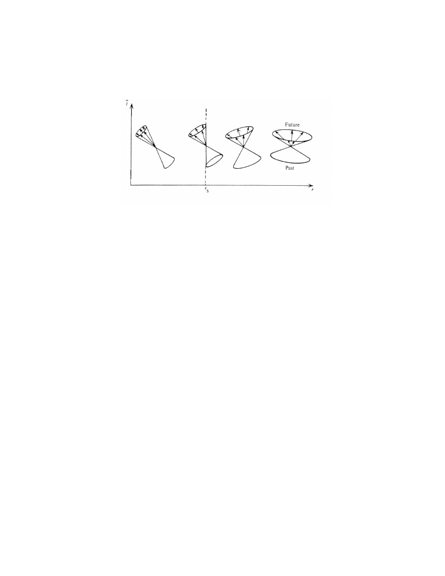
tilting over towards the black hole as we approach r = r
S
:
(Figure 46, page 93 of Principles of Cosmology and Gravitation, M.
Berry, Cambridge University Press, 1976.) Again, far from the black
hole, light cones are as they appear in flat spacetime. For r ≈ r
S
and
r > r
S
, light cones tilt over towards the black hole, but photons can
still escape the black hole. At r = r
S
, photons are either trapped at
r = r
S
(those emitted radially to the black hole) or are drawn into
the black hole. For r < r
S
, all worldlines are directed towards r = 0.
Therefore anything inside r
S
will be drawn to r = 0. All matter in a
black hole is therefore concentrated at r = 0 in a singularity of infinite
density.
Note. The Schwarzschild solution is an exact solution to the field
equations. Such solutions are rare, and sometimes are not appreciated
in their fullness when introduced. Here is a brief history from Black
Holes and Time Warps: Einstein’s Outrageous Legacy by Kip Thorne
(W.W. Norton and Company, 1994):
6

1915 Einstein (and David Hilbert) formulate the field equations (which
Einstein published in 1916).
1916 Karl Schwarzschild presents his solution which later will describe
nonspinning, uncharged black holes.
1916 & 1918 Hans Reissner and Gunnar Nordstr¨om give their solu-
tions, which later will describe nonspinning, charged black holes.
(The ideas of black holes, white dwarfs, and neutron stars did
not become part of astrophysics until the 1930’s, so these early
solutions to the field equations were not intended to address any
questions involving black holes.)
1958 David Finkelstein introduces a new reference frame for the Schwarz-
schild solution, resolving the 1939 Oppenheimer-Snyder paradox
in which an imploding star freezes at the critical (Schwarzschild)
radius as seen from outside, but implodes through the critical ra-
dius as seen from outside.
1963 Roy Kerr gives his solution to the field equations.
1965 Boyer and Lindquist, Carter, and Penrose discover that Kerr’s
solution describes a spinning black hole.
Some other highlights include:
1967 Werner Israel proves rigorously the first piece of the black hole
“no hair” conjecture: a nonspinning black hole must be precisely
spherical.
1968 Brandon Carter uses the Kerr solution to show frame dragging
around a spinning black hole.
7

1969 Roger Penrose describes how the rotational energy of a black hole
can be extracted.
1972 Carter, Hawking, and Israel prove the “no hair” conjecture for
spinning black holes. The implication of the no hair theorem is
that a black hole is described by three parameters: mass, rotational
rate, and charge.
1974 Stephan Hawking shows that it is possible to associate a tem-
perature and entropy with a black hole. He uses quantum theory
to show that black holes can radiate (the so-called Hawking radi-
ation).
1993 Hulse and Taylor are awarded the Nobel Prize for an indirect
detection of gravitational waves from a binary pulsar.
2002-2005 Gravity waves are directly detected with the Laser Inter-
ferometer Gravity Wave Observatory (LIGO).
8
Wyszukiwarka
Podobne podstrony:
Lugo G Differential geometry and physics (lecture notes, web draft, 2006)(61s) MDdg
Rajeev S G Geometrical methods in physics (lecture notes, web draft, 2004)(97s)
Freitag Several complex variables local theory (lecture notes, web draft, 2001)(74s) MCc
Rajeev S G Advanced classical mechanics chaos (Rochester lecture notes, web draft, 2002)(100s) PCtm
Walet N Further Maths 2C1 Lecture Notes(web draft, 2002)(79s) MCde
Introduction to Differential Geometry and General Relativity
Neumann W D Notes on geometry and 3 manifolds, with appendices by P Norbury (web draft, 2004)(54s)
Corporate Identity Image and Brands lecture notes
Ziming Li Lecture notes on computer algebra (web draft, 2004)(31s) CsCa
Gray R M Toeplitz and circulant matrices a review (web draft, 2005)(89s) MAl
Brizard A J Introduction to Lagrangian and Hamiltonian mechanics (web draft, 2004)(173s) PCtm
Field M , Nicol M Ergodic theory of equivariant diffeomorphisms (web draft, 2004)(94s) PD
Norbury General relativity and cosmology for undergraduates (Wisconsin lecture notes, 1997)(116s)
Lumiste Betweenness plane geometry and its relationship with convex linear and projective plane geo
Einstein A Relativity the special and general theory (free web version, Methuen, 1920) (115s)
Novikov S P Solitons and geometry (Lezioni Fermiane, Cambridge Univ Press, 1994, web draft, 1993)(50
więcej podobnych podstron