NBER WORKING PAPER SERIES

THE QUANTITY AND QUALITY OF LIFE AND

THE EVOLUTION OF WORLD INEQUALITY

Gary S. Becker

Tomas J. Philipson

Rodrigo R. Soares

Working Paper 9765

http://www.nber.org/papers/w9765

NATIONAL BUREAU OF ECONOMIC RESEARCH

1050 Massachusetts Avenue

Cambridge, MA 02138

June 2003

An earlier version of this paper circulated under the title “Growth and Mortality in Less Developed Nations.”
We benefited from comments of seminar participants at the 2002 AEA Meetings (Atlanta) and the World
Bank. Becker and Philipson received support from the George J. Stigler Center for The Study of The
Economy and The State. Becker received support from The John M. Olin Foundation and the NIHCD (Grant
#5401). The views expressed herein are those of the authors and not necessarily those of the National Bureau
of Economic Research.

©2003 by Gary S. Becker, Tomas J. Philipson, and Rodrigo R. Soares. All rights reserved. Short sections
of text not to exceed two paragraphs, may be quoted without explicit permission provided that full credit
including © notice, is given to the source.

The Quantity and Quality of Life and the Evolution of World Inequality
Gary S. Becker, Tomas J. Philipson, and Rodrigo R. Soares
NBER Working Paper No. 9765
June 2003
JEL No. I1, I3, J1, O1

ABSTRACT

Lack of income convergence for the world as a whole has led to concerns about the impact of

globalization of markets on world inequality. GDP per capita is usually used to proxy for the quality

of life of individuals living in different countries. However, well-being is also affected by quantity

of life, as represented by longevity. This paper incorporates longevity into an overall assessment of

the evolution of cross-country inequality. The absence of income convergence noticed in the growth

literature is in stark contrast with the reduction in inequality after incorporating recent gains in

longevity. The paper computes a "full" income measure to value the life expectancy gains

experienced by 49 countries between 1965 and 1995. Countries starting with lower income tended

to grow more in terms of "full" income than countries starting with higher income. The average

growth rate of "full" income is about 140% for developed countries, compared to 192% for

developing countries. Additionally, we decompose changes in life expectancy into changes

attributable to thirteen broad groups of causes of death. Infectious, respiratory and digestive

diseases, congenital and perinatal conditions, and "ill-defined" conditions are responsible for most

of the mortality convergence observed between 1965 and 1995.

Gary S. Becker

Tomas J. Philipson

Department of Economics

The Irving B. Harris Graduate School

University of Chicago

of Public Policy Studies

1126 E. 59th Street

University of Chicago

Chicago, IL 60637

1155 E. 60th Street, Suite 112
Chicago, IL 60637

Rodrigo R. Soares
Department of Economics
University of Maryland
3105 Tydings Hall
College Park, MD 20742

1

1 Introduction

Lack of income convergence for the world as a whole has led many people to be

worried about the impact of globalization of markets on world inequality. There is a fear

that although countries are getting richer, many developing countries are falling behind.

Many African countries, for example, have not experienced a significant growth in per

capita income during the last few decades, while OECD countries have grown

substantially. The absence of long run growth for some poor countries raises concerns

about whether development will reach all societies, or whether it will remain restricted to

only some countries.

Although GDP per capita is usually used as a proxy for the quality of life in

different countries, material gain is obviously only one of many aspects of life that

enhance economic well-being. Overall economic welfare depends on both the quality and

the quantity of life: yearly income and the number of years over which this income is

enjoyed. Recent estimates suggest that longevity has been a quantitatively important

component of the overall gain in welfare in the US during the twentieth century

(Nordhaus, 2003; Garrett, 2001; and Murphy and Topel, 2003). For example, Murphy

and Topel (2003) estimate that the average annual change in life expectancy in the US

between 1970 and 1990 had an aggregate value of approximately $2.8 trillion. These

annual gains corresponded to more than half of real GDP in 1980, and almost the same as

real consumption in that same year.

Given the quantitative importance of the value of gains in longevity in the US,

one wonders whether longevity gains are also an important part of the overall welfare

gains in the rest of the world. Incorporating longevity into an overall assessment of how

much cross-country inequality has grown may be important, as the absence of income

convergence noticed in the growth literature is in stark contrast with the evidence from

changes in life expectancy. As we show in this paper, there has been considerable

longevity-convergence: in the last 50 years, countries starting with modest longevity

levels experienced life expectancy gains significantly larger than countries starting with

high longevity levels.

2

This suggests that cross-country comparisons of changes in income per capita

may be misleading as indicators of changes in economic well-being. This paper tries to

account for the impact of longevity on the evolution of welfare across countries during

the last few decades. The use of per capita income to evaluate welfare improvements

assumes that it reflects the level of economic welfare enjoyed by the average person. We

extend the income accounts to incorporate survival rates throughout a person’s life. In

particular, we interpret per capita income as the income that the average individual in a

country would enjoy throughout his life, and interpret the survival rates for different ages

on a given year as determining the survival function of this average individual. This

allows us to analyze the impact of changes in survival probabilities on the welfare of this

hypothetical individual.

We use our longevity-adjusted income measure to reconsider what happens over

time to cross-country convergence and inequality. Our discussion refers to inequality

across different societies, as measured by differences in welfare of this hypothetical

individual. We do not consider the individual-level evolution of world inequality, as

recently done, for example, by Sala-i-Martin (2002).

This methodology is an extension of the original work of Usher (1973), which

was developed further by Rosen (1988). The approach allows us to give monetary values

to the longevity gains experienced by different countries between 1965 and 1995. These

estimated values, together with traditional per-capita income data, are then used to assess

the evolution of welfare in different countries, and the evolution of differences in welfare

across countries. Briefly, we compute the income gains that would represent welfare

improvements equivalent to the observed longevity gains. We analyze how the growth in

this “full” income, including both income per year and years enjoyed, changes the

traditional results regarding cross-country convergence. Our results indicate that

countries starting with lower income tended to grow more in terms of the “full” income

measure than countries starting with higher income. Using parameters from the value of

life literature, we estimate the per capita value of the longevity gains in terms of annual

income to be equivalent to 28% of the observed growth in per capita income for the US,

and more than 1.5 times the growth in per capita income for less-developed countries,

such as El Salvador, Chile, and Venezuela. More generally, the growth rate of the “full”

3

income measure in the thirty-year period examined has an average of 140% for

developed countries and 192% for developing countries.

We also disaggregate mortality data by causes of death to try to understand the

determinants of the cross-country convergence in life expectancy observed in the three

decades between 1965 and 1995. For each group of causes of death, we compute a

counterfactual measure of the mortality rate that would be observed in 1995 had mortality

rates by all causes but the one in question remained at their 1965 values. This approach

allows us to estimate the life expectancy gain attributable to reductions in mortality by

each specific cause of death. We show that changes in mortality due to infectious,

respiratory and digestive diseases, congenital and perinatal conditions, as well as “ill-

defined” conditions are the most important factors determining the convergence in life

expectancy. In other words, mortality of these causes of death fell more rapidly in poor

than in rich countries. At the same time, changes in mortality due to nervous system,

senses organs, heart and circulatory diseases worked against convergence, as mortality

for these causes fell more rapidly in rich rather than in poor countries. The large changes

in mortality observed in the developing world are consistent with the interpretation that

poor countries absorbed technology and knowledge previously available in rich

countries, at relatively low costs, while most of the changes in mortality in developed

countries took advantage of recent developments on the frontier of medical technology.

The structure of the paper is outlined as follows. Section 2 documents the recent

trends in longevity and per capita income growth, particularly the convergence in

longevity and the lack of convergence in per capita income. Section 3 discusses the

methodology used in the paper, and the parameterization and calibration of the model.

Section 4 uses these estimates to compute the value of welfare gains and the change in

inequality across countries, once life expectancy is accounted for. Of particular

importance here is the fact that poorer countries have gained more in longevity than

richer countries, so that the change in inequality in income per capita underestimates the

convergence in overall economic welfare. Section 5 decomposes the changes in life

expectancy into changes attributable to thirteen broad groups of causes of death. It shows

that recent patterns of mortality change differ greatly between developed and developing

countries. Also, it shows that a particular group of diseases is responsible for most of the

4

mortality convergence observed in the last thirty years. Lastly, section 6 summarizes the

main results and concludes the paper.

2 The Basic Trends: Post-War Convergence in Longevity and

Divergence in Income

The lack of income convergence across countries has been extensively

documented. This section reviews the evidence, calculates usual indicators of income

convergence for our data set, and analyzes whether there is cross-country convergence in

life expectancy. We concentrate on the changes observed between 1965 and 1995. The

mortality data are from the World Health Organization Mortality Database. Income

figures are from the Penn World Tables, version 6.0. The definition of the variables and

the countries included in the sample are contained in the Appendix.

1

2.1 Lack of Income Convergence

A vast literature has investigated whether poor countries tend to grow faster than

rich ones.

2

All these studies give virtually the same results.

3

Simple Gini coefficients,

regressions of growth rates on initial or final period incomes, standard deviations,

coefficients of variation, or indices of rank concordance do not show any evidence of

absolute convergence across countries (Park, 2000; Cannon and Duck, 2000; Boyle and

McCarthy, 1999; Quah, 1996; Barro and Sala-i-Martin, 1995; and Parente and Prescott,

1993). If anything, evidence suggests that rich countries tend to grow somewhat faster

than poor ones.

1

The sample includes 49 countries. These are the countries for which detailed mortality data by causes of

death are available for 1965 and 1995. Since this information is used for the calculations performed later
on in the paper, for consistency, we keep this same sample throughout. None of the results reported in this
section depend in any way on the sample. If anything, results tend to be stronger when a broader group of
countries is used (available from the authors upon request).

2

See, for example, the original contributions of Barro and Sala-i-Martin (1992) and Mankiw et al (1992).

For a discussion of the main results of this literature, see de la Fuente (1997), Quah (1996), and Barro and
Sala-i-Martin (1995).

3

There is still controversy in relation to how convergence should be measured: on beta and sigma

convergence see Barro and Sala-i-Martin (1995), on Galton’s fallacy see Cannon and Duck (2000).

5

Our data replicates the most commonly cited results of this literature. The income

statistic used is GDP per capita adjusted for terms of trade in international prices (from

now on, GDP). Table 1 presents standard deviations and coefficients of variation for

GDP and ln(GDP), in 1965 and 1995. All measures of dispersion either stay constant or

increase. Overall, the cross-country dispersion of income does not seem to have

decreased in the thirty years between 1965 and 1995.

But, since Galton, it is well known that a falling variance over time – i.e. reduced

cross-sectional inequality – is not the same thing as regression to the mean – i.e. poor

countries growing faster than rich ones. To explore this point, Figure 1 shows the result

of a regression of the increase in the natural logarithm of GDP between 1965 and 1995

(or growth rate of GDP, ln(GDP95/GDP65)), on the natural logarithm of the initial

income level (ln(GDP65)). The coefficient of ln(GDP65) is negative (-0.13), but not

statistically significant.

4

Besides, the correlation between the two variables is very small,

as reflected in the R

2

of only 0.04. Poor countries do not seem to grow faster than rich

ones. So evidence from our data set replicates the well-known result that there is no

income convergence across countries, whether interpreted as falling cross-sectional

inequality or growth rates conditional on initial levels.

2.2 Longevity Convergence

In contrast with the evidence for per capita income, convergence in life

expectancy has been taking place. Countries starting with low longevity tended to gain

more in life expectancy than countries starting with high longevity. We use the same

techniques common to the growth convergence literature to demonstrate this for life

expectancy at birth.

Table 1 presents standard deviations and coefficients of variation for life

expectancy at birth (from now on, Life), in the years 1965 and 1995. Both measures of

dispersion fall greatly in this thirty-year period. The coefficient of variation falls by 44%,

4

As discussed by Friedman (1992) in another context, zero-mean measurement error in the initial period

income tends to generate a spurious negative correlation between income per capita in 1965 and growth
rate in the following thirty years. This correlation biases the coefficient of the regression towards negative
values, artificially increasing the measured degree of convergence. Nevertheless, even with the bias

6

from 0.075 to 0.042. There has been a significant reduction in the cross-country

dispersion of longevity between 1965 and 1995.

Figure 2 presents the result of a regression of the gains in life expectancy at birth

between 1965 and 1995 (Life95 – Life65) on the initial level of life expectancy (Life65).

The coefficient on Life65 is negative and statistically significant at any conventional

significance level.

5

The point estimate implies that, on average, each additional 10 years

of life expectancy in 1965 represented a reduction of more than 6 years in life expectancy

gains in the following 30 years.

2.3 The Changing Relation between Income and Longevity

The previous evidence shows that, while there is no convergence in per capita

income across countries, there is convergence in longevity. Since at any point in time

there is a positive correlation between longevity and per capita income, this cross-

sectional relation must be shifting over time.

For given levels of income, longevity has been rising, and this increase has been

greater for poor countries. The shift in this cross-sectional relation was first noticed by

Preston (1975), who analyzed data between 1930 and 1960. He showed that, holding

income constant, the shift in the longevity-income profile represented gains of up to 15

years in life expectancy. Our data shows that this phenomenon is still taking place. Figure

3 plots life expectancy levels for 1965 and 1995 against per capita GDP for the same

years, and fits a logarithm function to each year. For constant levels of income, life

expectancy has been rising. This rise has been more than 5 years for poor countries.

6

towards convergence, it is not uncommon for one to obtain a positive and marginally significant coefficient
in this regression when a larger sample of countries is used.

5

The point raised in footnote 4 does not apply here. It is widely accepted that life expectancy numbers for

developing countries are probably overestimated, since number of deaths in remote areas (where there is
not much presence of the state) are likely to be underreported. In this case, measurement error in the initial
period does not have zero mean. Also, it seems reasonable to assume that record keeping practices have
improved in the last thirty years, and evidence presented in section 5 supports this idea. If that is the case,
developing countries would have a systematically positive measurement error in life expectancy, and this
error would be systematically larger in 1965. Therefore, the regression of changes in life expectancy on
initial levels would bias the convergence coefficient towards positive values. True convergence should be
even higher than the one measured in Figure 2. The measurement error in life expectancy is likely to work
against all the main results discussed in the paper.

6

Again, these features of the data are intensified when a larger sample of countries is used.

7

Measurement error could potentially explain part of this shift. If life expectancy is

determined by permanent income, but we observe permanent income plus a transitory

error, a way to estimate the “permanent” slope would be to compare life expectancy and

income at the means in each year. Assuming a stable ‘permanent income-life expectancy’

profile throughout the period, we can calculate the largest life expectancy gain that could

be potentially explained by changes in income. This strategy attributes the shift to

measurement error, and implicitly assumes that all changes in life expectancy were

determined by changes in permanent income.

By applying this methodology to our dataset, we find the coefficient of the

relation between life expectancy and the natural logarithm of income per capita to be 9.7,

more than two times larger than the coefficients estimated in the regressions from Figure

3. But additional evidence suggests that measurement error cannot account for the whole

story. First, this estimated coefficient generates systematic differences in prediction

errors between developed and developing countries that are not compatible with the

simplest version of the measurement error hypothesis: life expectancy gains are, on

average, underestimated for developing countries and overestimated for developed

countries. If measurement error in income was behind the observed shift, we should

expect just the opposite. In addition, the cross-sectional relationship between life

expectancy and other demographic variables – such as educational attainment and

fertility – is more stable over time (see, for example, Soares, 2003). To the extent that

these variables are usually thought to be measured less precisely than income, it is

difficult to argue that the entire shift in the income-life expectancy profile should be

attributed to measurement error.

Together with the evidence presented in Preston (1975), Figure 3 suggests that the

cross-sectional relation between income and longevity has been shifting constantly since

the beginning of the twentieth century. Longevity gains have been taking place in all

income ranges, with particular intensity in medium and lower levels. In fact, this

changing relationship explains the contradicting trends in terms of life expectancy

convergence vis-à-vis income convergence. If we only consider the component of the

change in life expectancy explained by changes in income, there is no convergence.

8

This point is explored in Figure 4, where we simulate the life expectancy level

that would be observed in 1995, had the 1965 income-life expectancy profile remained

stable throughout the period. In other words, using the regression estimated in Figure 3,

we simulate the 1995 life expectancy level as: L’

95

= L

65

+ 4.05(lny

95

– lny

65

), where L

denotes life expectancy at birth, and y denotes income per capita. This simulates the life

expectancy that would be observed in 1995 if all the changes in this variable between

1965 and 1995 were driven by changes in income, with the 1965 income-life expectancy

profile remaining stable. Figure 4 shows that, once we look only at the component of life

expectancy changes explained by changes in income, there is no convergence. If

anything, the Figure suggests that the dimension of life expectancy correlated with

income tended to increase cross-country dispersion. Convergence in life expectancy

seems to be driven by changes that are actually orthogonal to changes in income.

Since life expectancy is an important dimension of welfare, the evidence

discussed in this section indicates that it could be misleading to analyze the evolution of a

country’s economic well-being – or the difference in well-being across countries – based

solely on income indicators. In the next section, we develop a methodology to

incorporate longevity into the analysis of the cross-country evolution of welfare and

inequality.

3 Adding the Two Trends: Monetizing the Value of Longevity Gains

To incorporate life expectancy gains into the analysis, we must be able to express

these gains and income gains into the same units. With this goal, we draw from the

literature on the economic value of risks to life (for an overview of this literature, see

Viscusi, 1993). Estimates for the US suggest that gains in longevity between 1970 and

1990 represented welfare improvements comparable to the material gains observed in the

same period, and that historical reductions in mortality were also major sources of

welfare improvements (see Cutler and Richardson, 1997; Nordhaus, 2003; Murphy and

Topel, 2003; and Garrett, 2001).

9

3.1 Converting Longevity Gains into their Income Value

Previous work of Usher (1973), Rosen (1988), and Murphy and Topel (2003),

derive the utility parameters of interest that determine the marginal willingness to pay for

longevity gains. Given the infra-marginal changes in longevity and income observed

during the long time period we analyze, we derive the analog infra-marginal expressions

that do not rely on marginal approximations. Consider the indirect utility function V(Y,S)

of an individual with survival function S and lifetime full income Y:

7

∫

∞

−

=

0

))

(

(

)

(

)

exp(

max

)

,

(

dt

t

c

u

t

S

t

S

Y

V

ρ

(1)

subject to

,

0

)

(

)

(

)

exp(

0

)

(

)

(

)

exp(

∫

∫

∞

−

=

∞

−

=

dt

t

c

t

S

rt

dt

t

y

t

S

rt

Y

(2)

where y(t) is income at age t, c(t) consumption at t, and r is the interest rate; and where

the budget constraint assumes the existence of a complete contingent claims market.

Now consider a given country at two points in time, τ and τ + ∆τ, with lifetime

income and survival functions denoted Y

τ

and S

τ

, and Y

τ+∆τ

and S

τ+∆τ

. We are interested in

the infra-marginal income that would give a person in this country the same utility level

observed in period τ + ∆τ, but with the mortality rates observed in period τ. This income

equivalent compensation E would satisfy

V(E + Y

τ+∆τ

,S

τ

) = V(Y

τ+∆τ

,S

τ+∆τ

).

(3)

Figure 5 illustrates the exercise in terms of indifference curves of the indirect

utility function on the (Y,T) plane, for the case of a deterministic lifetime equal to T. We

slide in the indifference curve of period τ + ∆τ to the longevity observed in period τ; the

income at that point is E + Y

τ+∆τ

.

More formally, we abstract from life cycle considerations by assuming that r =

ρ

,

y(t) is constant (y(t) = y), and the individual has access to a fair insurance (as expressed

7

When the context is clear, we save on notation by writing the survival function as S, instead of S(t).

10

in the budget constraint). With these assumptions, it is well known that optimal

consumption c(t) is also constant, so that c(t) = c = y. This implies that the indirect utility

function can be expressed in terms of the yearly income y as

.

)

(

)

exp(

)

(

)

,

(

0

∫

∞

−

=

dt

t

S

rt

y

u

S

y

V

(4)

Define

A(S) as the value of an annuity based on the survival function S, such that

∫

∞

−

=

0

)

(

)

exp(

)

(

dt

t

S

rt

S

A

. If e is the yearly – as opposed to lifetime – income that

compensates for lower longevity in a manner similar to before, e satisfies

u(e + y

τ+∆τ

)A(S

τ

) = u(y

τ+∆τ

)A(S

τ+∆τ

).

(3’)

With a first order Taylor expansion of u(.) around y

τ+∆τ

to approximate

u(e + y

τ+∆τ

), one obtains u(e + y

τ+∆τ

) ≈ u(y

τ+∆τ

) + u' (y

τ+∆τ

)e. Substituting for u(e + y

τ+∆τ

)

from expression (3’) above and rearranging terms, yields:

;

)

(

)

(

)

(

)

(

1

,

)

(

)

(

)

(

)

(

'

)

(













−

=













−

=

∆

+

∆

+

∆

+

∆

+

∆

+

∆

+

τ

τ

τ

τ

τ

τ

τ

τ

τ

τ

τ

τ

τ

τ

τ

τ

ε

S

A

S

A

S

A

y

y

e

or

S

A

S

A

S

A

y

u

y

u

e

(5)

where

ε

(.) is the elasticity of the instantaneous utility function in relation to its argument.

Though we will not make use of linear approximations in our empirical analysis,

this expression neatly illustrates the main determinants of the value of longevity gains. In

short, the value rises with the degree of inter-temporal substitution and the percentage

(discounted) longevity gain. More specifically, two dimensions summarized in this

expression will be very important in our analysis: the level of income (or consumption)

throughout life (term outside brackets), and the size and moment of the reductions in

mortality (term inside brackets). Whenever income and longevity are positively

correlated across countries, the willingness to pay for an increase in life expectancy will

11

generally have two offsetting components. Richer countries attach more value to given

longevity gains (higher u(y

τ+∆τ

)/u'( y

τ+∆τ

)), and countries with higher longevity attach less

value to given absolute longevity gains (higher A(S

τ

); see Dow et al, 1999). The effect of

income comes from the fact that marginal extensions in life expectancy are more valuable

the higher is consumption in this extended lifetime, or, in other words, the higher is the

income level.

Income can be used to measure material improvements only with a set of

assumptions that justify using a single number to portray changes in a country’s welfare.

Similar simplifying assumptions are needed to measure the material value equivalent to

the life expectancy gains observed in a certain period. More precisely, we interpret per

capita income from national accounts as the income that the average individual would

enjoy throughout his life, and use survival rates for different ages in a given year to

determine the survival function this individual would experience. From now on, when

talking about economic welfare, we refer to this hypothetical individual, who would face

the survival probabilities corresponding to the country’s cross-sectional life expectancy

at birth, and would earn in every period of life an income equal to the country’s per

capita GDP in that year. This allows for the calculation of the value of gains in life

expectancy using only national income and mortality statistics widely available. For this

same reason, the usual critiques of GDP as a measure of full income – due to the fact that

it does not incorporate value of leisure, household production, and non-traded goods –

also apply to our methodology. In fact, what we do is to try to fill in one of these gaps.

Our argument is similar to the one contained in the usual growth discussions

based on income alone, as they too implicitly assume that GDP per capita reflects in

some way the level of economic welfare enjoyed by the average person. We just extend

this interpretation to take into account survival rates across the average person’s life. This

methodology allows us to discuss the evolution of welfare inequality across countries, by

analyzing the changes in welfare of this representative individual. We do not discuss the

individual-level evolution of world inequality, as done, for example, by Sala-i-Martin

(2002).

12

3.2 The Income Value of Cause Specific Mortality Reductions

Consider

K competing causes of mortality, represented by the survival functions

in S = S

1

S

2

S

3

…S

K

=

∏

=

K

k

k

S

1

. Following the same steps as in the previous section, define the

value (in annual income) of the longevity gain associated with the k

th

cause of death as

the e

k

implicitly determined by the following expression

8

u(e

k

+ y

τ+∆τ

)A(S

τ

) = u(y

τ+∆τ

)A(S*

k

τ+∆τ

),

(6)

where

∏

=

≠

∆

+

∆

+

k

i

i

k

k

S

S

S

τ

τ

τ

τ

τ

*

.

(7)

S*

k

τ+∆τ

is a counterfactual survival function, simulating the survival function that

would exist in period τ +∆τ, had the mortality rates for all causes of death but k remained

at their τ period levels. In other words, it simulates what the survival function in τ +∆τ

would be if only the changes observed in the k

th

cause of death had taken place.

This strategy allows the decomposition of the gains in life expectancy observed in

any given period into K different causes. But, given that changes in mortality from

different causes interact with each other in generating the final survival function, this

decomposition does not explain exactly 100% of the shift in this function when infra-

marginal changes in mortality are being considered (this is the competing risks nature of

mortality rates, as discussed by Dow et al, 1999). Formally, this strategy is a first order

decomposition of changes in the survival function into changes in its K components. For

marginal changes in S through time, this approach would indeed generate an exact

decomposition, as in

8

In terms of the first order approximation using the Taylor expansion, the expression for e

k

would be













−

=

∆

+

∆

+

∆

+

)

(

)

(

)

*

(

)

(

'

)

(

τ

τ

τ

τ

τ

τ

τ

τ

S

A

S

A

S

A

y

u

y

u

e

k

k

.

(6’)

13

∑ ∏

=

≠













∂

∂













=

∂

∂

K

i

i

i

k

k

S

S

S

1

τ

τ

.

(8)

Note that each term in the sum is exactly the change in the survival function due

to each cause of death that would be obtained using our counterfactual measure S*

k

τ+∆τ

:

k

k

i

i

k

k

k

i

i

k

S

S

S

S

S

S

S

∆













=

−













=

−

∏

∏

≠

∆

+

≠

∆

+

τ

τ

τ

τ

τ

τ

τ

τ

)

(

*

. So, with marginal changes in mortality

rates,

∑

=

=

K

k

k

e

e

1

.

But with infra-marginal changes, higher order terms due to the complementary

nature of mortality rates are also relevant. Nevertheless, we stick to the first order

decomposition of changes in survival functions to simplify the discussion, and because

due to the interaction among these higher order terms, it is impossible to attribute their

effects to any particular cause of death.

9

S*

k

τ+∆τ

allows us to construct a counterfactual life expectancy measure that

simulates the life expectancy that would be observed in τ + ∆τ if only the changes in

mortality due to the k

th

cause of death had actually taken place. As discussed in the

empirical section, this counterfactual life expectancy measure can be used to decompose

the convergence in life expectancy into K underlying mortality causes, plus a higher

order term (due to interactions between different causes of death).

3.3 Parameterization of the Model

To calculate the economic value of the longevity gains observed between 1965

and 1995, and decompose it into the value attributable to each different cause of death,

we need data on per capita income (y), survival rates (S), and a specific functional form

for the utility function (u(.)). Two dimensions of the instantaneous utility function u(.) are

relevant. The willingness to pay for extensions in life expectancy is affected both by the

substitutability of consumption in different periods of life, i.e. the inter-temporal

elasticity of substitution, and by the value of being alive relative to being dead.

10

9

As discussed in the empirical section, these first order terms account for more than 80% of the changes in

life expectancy in the dataset.

10

This is related to the state-dependent nature of this problem, and to the normalization of utility in the

death state to zero (discussed in detail by Rosen, 1988).

14

We abstract from leisure throughout the paper, and allow the following functional

form for the instantaneous utility function to capture these two different dimensions:

α

γ

γ

+

−

=

−

/

1

1

)

(

/

1

1

c

c

u

,

(9)

where α is the parameter that arises from the normalization of utility in the death state to

zero, and γ is the inter-temporal elasticity of substitution. The parameter

α

determines the

level of annual consumption at which the individual would be indifferent between being

alive or dead. If that level were positive, an inter-temporal elasticity

γ

larger than 1 would

imply that

α

would be negative.

The

parameter

α

can be identified from other parameters more commonly

estimated in the value of life literature. More precisely, we have that

α

γ

ε

γ

γ

+

−

=

=

−

−

/

1

1

)

(

)

(

'

/

1

1

/

1

1

c

c

c

u

c

c

u

,

(10)

and, from this expression,













−

−

=

−

γ

ε

α

γ

/

1

1

1

1

/

1

1

c

.

The value of

ε

can be estimated from compensating differentials for occupational

mortality risks. Murphy and Topel (2003, p.23), using numbers from the literature on

occupational risks, estimate

ε

to be 0.346.

A wide range of values is available in the empirical literature on the inter-

temporal elasticity of substitution. Browning, Hansen, and Heckman (1999, p.614), after

exhaustively reviewing the estimates, suggest that the inter-temporal elasticity of

substitution for non-durables is probably slightly above 1.

We use γ = 1.25,

ε

= 0.346 and c = $18,000 to calibrate the value of

α

. The value

of consumption is the value of US per capita income in 1990 in our data set, the year in

which Murphy and Topel (2003) estimate

ε

using US data. Our calculations give a value

of

α

equal to -14.97. Together with the value of

γ

, this means that an individual with

15

annual income equal to 241 would be indifferent between being alive or dead.

11

Following Murphy and Topel (2003), we set interest rates to 3% per year.

12

With these values of α and γ, we can use equation (3’) to value the life expectancy

gains experienced by the different countries in the thirty year period between 1965 and

1995. With all assumptions,

13

τ

τ

γ

γ

τ

τ

τ

τ

τ

τ

τ

γ

τ

τ

γ

α

∆

+

−

∆

+

∆

+

−

∆

+

−





























−

−

+

=

y

S

A

S

A

S

A

S

A

S

A

y

e

1

/

1

1

)

(

)

(

)

(

)

1

1

(

)

(

)

(

.

(11)

Again,

e gives the additional flow of annual income that would generate a welfare

gain comparable to the one generated by the increase in survival probabilities observed

during the period. An analogous expression is used to calculate the annual income value

of the reductions in mortality due to each particular cause of death. In this case, we

substitute e by e

k

, and S

τ+∆τ

by S*

k

τ+∆τ

.

We also use e to calculate what we call the growth rate of the income equivalent

compensation, given by

1

−

+

=

∆

+

τ

τ

τ

y

e

y

g

. This concept gives the income growth rate that

would have been observed had all the welfare gain in the period taken the form of income

growth.

4 The Effect on World Inequality

We use expression (11) to calculate the value of the longevity gains observed in

49 countries between 1965 and 1995, and to evaluate the impact of the changes in

longevity on cross-country inequality. Per capita income figures are taken from the Penn

11

The lowest value of the GDP per capita variable (adjusted for terms of trade, RGDPTT) in the PWT 6.0

dataset is 275.93, for the Democratic Republic of Congo in 1997. Also, this is the only observation in the
whole PWT 6.0 dataset with value below 300.

12

When presenting the results, we briefly discuss the effects of assuming a higher interest rate.

13

The formula used in the calculations is a discrete time version of (11). A cleaner version of this

expression can be obtained if we use the linear approximation from the Taylor expansion. In this case, we
have:













−















−

−

=

∆

+

−

∆

+

)

(

)

(

)

(

1

/

1

1

τ

τ

τ

τ

γ

τ

τ

α

γ

γ

S

A

S

A

S

A

y

e

.

(11’)

Since we have a closed form solution for e, there is no reason to use this simpler linear approximation.

16

World Tables 6.0. Data are ten-year averages centered in the reference years: 1965

corresponds to the average for the period between 1960 and 1969, and 1995 corresponds

to the average between 1990 and 1999 (or years available in these intervals).

Survival rates are constructed using age specific number of deaths and population

from the World Health Organization Mortality Database. Mortality rates are assumed to

be constant inside the age intervals for which data is tabulated. Figure 6 illustrates the

extent of variation in age specific mortality rates in the dataset, by plotting two extreme

examples: the survival distribution for Egypt in 1965 (lowest life expectancy at birth in

the sample), and the survival distribution for Japan in 1995 (highest life expectancy at

birth in the sample).

Table 2 presents the results for the value of longevity gains and the growth rate of

the income equivalent compensation, together with other income and life expectancy

statistics, using the value of the parameters derived in the previous section. The value of

longevity gains is presented in two forms: annual income (e), and total discounted

lifetime value (E).

14

Results are presented for individual countries and as un-weighted averages for

groups of developed and developing countries. Developed countries include countries

from North America, Western Europe, and Australia, New Zealand, and Japan, whereas

developing countries include countries from Latin America, Eastern Europe, Southeast

Asia, and Africa.

15

On average, the value of longevity gains in terms of annual income is somewhat

higher for developed countries: $1,747 against $1,265 (in international prices). But the

14

Remember that E is the present discounted value of the flow of income e, taking into account both the

interest rate and the survival probabilities in the initial period (τ = 1965):

∫

∞

−

=

0

)

(

)

exp(

dt

t

S

rt

e

E

τ

= eA(S

τ

).

15

The classification into groups of developed and developing countries inevitably involves some degree of

arbitrariness. We try to do so in a way that does not bias the aggregate results in our favor. If anything, our
grouping will work towards reducing longevity convergence between developing and developed countries.
This is because our developed countries include countries such as Portugal, Spain, Greece, and Ireland, that
were not developed in the 1960’s and that experienced impressive life expectancy gains in the period. At
the same time, our developing countries include Eastern European countries such as Bulgaria,
Czechoslovakia, Hungary, and Romania, that had high life expectancy at 1965 and that experienced
virtually no gain in this variable during the following period, partly as a consequence of the collapse of the
communist block.

17

highest values of this variable are in the developing world: Chile, Hong Kong, and

Singapore experienced longevity gains with values superior to $3,200 in annual income.

This gain corresponds to 90% of the Chilean GDP per capita in 1965, while the gains for

Hong Kong and Singapore are more than 118% of their GDP’s per capita in 1965.

Longevity gains are more important for developing countries in terms of average

annual value as a percentage of the GDP. These gains correspond to 55% of the 1965

GDP per capita for the less-developed world, and only 29% for the developed world.

This tendency is reflected in the growth rate of the income equivalent compensation. In

this case, since the initial income level is lower for developing countries, the difference

between developing and developed countries is reversed: the average growth for

developing countries is 192%, against 140% for developed countries.

This indicates that, unlike income changes, longevity changes since 1965 reduced

the disparity in welfare across countries. Figure 7 explores this point further by plotting

the growth rate of the income equivalent compensation against the natural logarithm of

GDP per capita in 1965. As the Figure shows, the inclusion of life expectancy in the

measure of welfare tends to increase the convergence in the period. The coefficient on

ln(GDP65) is negative and statistically significant. Higher income in 1965 is consistently

associated with lower growth in “full” income in the thirty-year period between 1965 and

1995.

16

The ideal independent variable in the right-hand side of this regression should be

a measure of “full income in 1965.” Since the approach discussed in section 3 does not

allow us to calculate the value of given levels of life expectancy, but only the value of

changes in life expectancy, we are forced to use the 1965 value of income per capita

rather than “full income.” Using some measure of full income in this regression would

unambiguously increase the degree of convergence since richer countries in 1965 also

had higher life expectancy.

16

Using a higher interest rate reduces the overall willingness to pay for reductions in mortality because of

the heavier discounting of future gains in longevity. But it does not change the qualitative results regarding
convergence. For example, with r = 0.07 – roughly the rate of return on capital in the US – the average
growth rate of the income equivalent compensation becomes 118% for developed countries, and 145% for
developing countries. In the cross-country convergence regression, the coefficient on income per capita in
1965 increases slightly in absolute value, to –0.21 (with p-value = 0.02).

18

These results indicate convergence in welfare, in the sense that countries with

higher initial income tended to have significantly lower subsequent welfare gains (in

terms of “full income”). Incomes 100% higher in 1965 were associated, on average, with

income equivalent growth rates 20% lower in the following 30 years. This result is not

surprising, given the negative correlation between life expectancy gains and income. As

long as the income elasticity of value of life is not much above unity, any value attached

to longevity would work towards increasing convergence. Viscusi and Aldy (2003)

conclude, from various types of evidence, that this elasticity is less than unity, but their

results for countries are greatly affected by a couple of extreme observations for India.

Without these observations, Becker and Elias (2003) get an elasticity of about unity.

Figure 8 shows, for each country in the sample, the share of the welfare

improvements observed between 1965 and 1995 due to mortality reductions. This share is

calculated as value of longevity gains in annual income/(value of longevity gains in

annual income + increase in annual income between 1965 and 1995). The average value

across countries is 27%, meaning that recent welfare gains due to mortality reductions

average about 1/3 of the material gains observed in the same period. In some cases, like

Chile, Ecuador, Egypt, El Salvador, and Venezuela, longevity gains have been by far the

most important factor in determining the welfare improvements observed after 1965. As

the Figure suggests, this share is systematically related to income: on average, poorer

countries had a higher share of welfare gains due to longevity increases (the coefficient

of a regression of the share of welfare gains due to longevity on lny

65

is equal to –0.079

with p-value = 0.03).

Overall, the evidence shows that longevity changes in the period between 1965

and 1995 worked towards reducing the disparity in welfare across countries. The actual

reduction in disparity depends on the specific values of the parameters

α

and

γ

; that is, on

the relative importance of quantity and quality of life. But, nevertheless, the qualitative

role played by mortality reductions in the process should be obvious.

These results would be even stronger if we accounted for expenditures on health

and R&D, because part of the gains in life expectancy is driven by expenditures on health

and R&D. Since most of these expenditures are undertaken by the developed world, the

share of truly exogenous reductions in mortality is certainly higher for the less-developed

19

countries.

17

Therefore, convergence in welfare would be higher if the endogenous part of

longevity gains were netted out.

5 The Causes of Mortality Convergence

Cross-country life expectancy convergence would follow if the health production

technology were concave, as illustrated by the logarithmic curves in Figure 3. Countries

with higher initial mortality then would have larger mortality reductions because they

have much higher returns on investments in health than do countries with lower

mortality.

However, some evidence hints that this is not the full story. Figure 3 shows a

possible shift in the relation between income and life expectancy, suggesting that a

considerable part of the changes in longevity is related to technological improvements.

Stable concave returns to investments in health cannot account for this evidence, as

Figure 4 clearly illustrated. Moreover, since investments in health are much larger for

developed than for developing countries – measured either in absolute terms or as shares

of income (see footnote 17) – a stable health production function could not explain the

convergence in life expectancy, unless returns to investments in health were much higher

for the less-developed world.

5.1 Data

To understand the nature of the changes in mortality in the developing world, we

decompose the gains in life expectancy into different causes of death. The World Health

Organization Mortality Database contains number of deaths by cause of death for the

years under analysis. Causes of death in the different years are classified according to the

current International Classification of Diseases (ICD) code, so data for different periods

has to be made compatible by matching codes of the different versions of the ICD. As we

17

For example: in 1995, health expenditures per capita in the US and Sweden were around US$4,000; in

the same year, these expenditures were between US$100 and US$200 for Mexico, Poland, and Turkey. In
terms of share of per capita GDP, this corresponded to 14% and 9% for, respectively, US and Sweden, and
below 5% for Mexico, Poland, and Turkey (data from the World Bank Development Indicators). These
numbers are representative of the patterns observed in other developed and developing countries.

20

will be dealing with rather broad groups of causes of death, this will not be much of a

problem.

We define the following thirteen groups of causes of death: R01: infectious

diseases; R02: neoplasms; R03: endocrine, metabolic and blood diseases, and nutritional

deficiencies; R04: mental disorders; R05: diseases of the nervous system and senses

organs; R06: heart and circulatory diseases; R07: respiratory and digestive diseases; R08:

urinary and genital diseases; R09: abortion and obstetric causes; R10: skin and

musculoskeletal diseases; R11: congenital anomalies and perinatal period conditions;

R12: ill-defined conditions; and R13: accidents, suicides and homicides. The grouping of

the codes from the ICD-6/7 and ICD-9 into these thirteen categories is described in the

Appendix.

5.2 Convergence Decomposition

To evaluate the contribution of each cause of death to the observed reductions in

mortality, we use the counterfactual survival function S*

k

τ+∆τ

defined in section 3.2. To

recapitulate, we construct, for each cause of death, the survival function that would have

been observed in 1995 had mortalities of all causes but the one in question remained at

their 1965 levels.

18

Or, in other words, we simulate what mortality levels would have

been observed in 1995 if only the changes in one of the causes of death had actually

taken place.

With the cause specific survival functions S*

k

τ+∆τ

, we can immediately construct

corresponding cause specific counterfactual measures of life expectancy, each one

defined as

∫

∞

∆

+

∆

+

=

0

)

(

*

*

dt

t

S

L

k

k

τ

τ

τ

τ

. L*

k

τ+∆τ

is the exact analog of S*

k

τ+∆τ

in terms of life

expectancy. For our purposes, it gives the life expectancy that would be observed in 1995

if only mortality rates due to the k

th

cause of death had actually changed between 1965

and 1995.

18

Specifically, to compute the survival function S*

k

95

, we use age specific mortality rates for the k

th

cause

of death calculated using 1995 populations and number of deaths, and age specific mortality rates for all
the other causes of death using 1965 populations and number of deaths.

21

This strategy allows the decomposition of the gains in life expectancy observed in

the period into the thirteen different groups of causes of death defined before, plus a

higher order term (see discussion in section 3.2). Let L

τ

denote life expectancy at birth in

year τ. Then

∆L = ∆L

1

+ ∆L

2

+ …+ ∆L

13

+ ∆L

H

,

(12)

where ∆L is the change in life expectancy observed between 1965 and 1995; ∆L

k

, for k =

1,…,13, is the change in life expectancy attributable to the k

th

cause of death, defined as

∆L

k

= L*

k

95

– L

65

; and ∆L

H

is the change in life expectancy due to the interaction

between mortality changes in the thirteen groups (higher order terms).

Our goal is to decompose the convergence in life expectancy into convergence in

mortality in each one of the thirteen causes of death. By definition, the coefficient

indicating convergence in life expectancy is given by the coefficient of a linear

regression of ∆L on a constant plus L

65

. Define X

65

= [1 L

65

], a matrix containing a

column of ones, and a column with the life expectancy at birth for the different countries

in the sample in 1965. The convergence coefficient is given by

β

= (X

65

’X

65

)

-1

X

65

’∆L

(13)

By

substituting

∆L from expression (12), we can write

β

= (X

65

’X

65

)

-1

X

65

’(∆L

1

+

∆L

2

+ …+ ∆L

13

+ ∆L

H

). This expression gives a natural decomposition for the

convergence coefficient:

β

= (X

65

’X

65

)

-1

X

65

’(

∑

=

∆

13

1

k

k

L + ∆L

H

) =

β

1

+

β

2

+ …+

β

13

+

β

H

,

(14)

where

β

i

, for i = 1, …, 13, H, is the coefficient of the OLS regression of ∆L

i

on X

65

.

In words, the coefficient of the regression of changes in life expectancy on initial

life expectancy levels can be decomposed into coefficients of regressions of cause

specific changes in life expectancy on initial life expectancy levels, plus a residual term

22

(β

H

). That is, convergence in life expectancy is decomposed into convergence attributable

to the thirteen underlying causes of death, plus a residual term. This allows us to evaluate

the role of different causes of death in generating the observed convergence in life

expectancy.

Table 3 presents the results of regressions of the changes in life expectancy

attributable to a particular cause of death on the initial life expectancy level (the

β

i

coefficients). The Table also presents the R

2

of the regressions and the contribution of the

specific cause of death to the overall life expectancy convergence (

β

i

/

β

).

The behavior of the regression coefficient is very different across the different

causes of death. Out of the thirteen coefficients, six are positive, meaning that the

behavior of mortality due to these six causes of death worked against life expectancy

convergence. Most of these six “divergent” causes of death had virtually no impact on

overall convergence, but two played a considerable role in reducing convergence:

mortality by nervous system, senses organs, heart, and circulatory diseases reduced

convergence by more than 20% of its actual value. In the case of nervous system and

senses organs diseases, mortality reductions were experienced by both developed and

developing countries, but the extent of these reductions was considerably larger for

developed countries. In terms of heart and circulatory diseases, mortality reductions were

also considerable for developed countries, but basically nonexistent for most of the

developing world.

In the case of the causes of death that worked towards increasing convergence,

the action is concentrated in a handful of cases: infectious, respiratory and digestive

diseases, congenital anomalies, perinatal period conditions, and ill-defined conditions

accounted for roughly 110% of the observed convergence. Among these, respiratory and

digestive diseases were by far the most important, accounting for 60% of the

convergence. Note that this group includes infectious diseases related to the respiratory

tract, such as pneumonia and influenza, and digestive tract diseases such as appendicitis

and cirrhosis. The second most important contribution to convergence comes from “ill-

23

defined” causes and conditions. This most likely reflects the relative improvement of

medical practice and record keeping behavior in developing countries.

19

These results support the view that recent reductions in mortality in the

developing world have been due in part to the absorption of previously available

technologies (for arguments in this direction, see Preston, 1980; and Soares, 2003). The

group of infectious, respiratory and digestive diseases, congenital anomalies, and

perinatal period conditions includes the types of diseases for which educational health

programs and simple interventions can have large beneficial effects. On the other side of

the spectrum, developed countries benefited relatively more from reductions in mortality

that required new technological developments, relatively costly change of habits, and

expensive surgical interventions (heart, circulatory, and nervous system diseases). The

concept is of a developed center that generates health and medical knowledge to be

absorbed eventually by the underdeveloped periphery.

5.3 Value of Longevity Gains Decomposition

Using the methodology described in section 3.2, we decompose the value of life

expectancy gains into gains attributable to the thirteen causes of death. The value of life

expectancy gains attributable to each particular cause of death is calculated using

survival rates which assume that only mortality due to one cause of death changed

between 1965 and 1995.

Table 4 presents the total value of longevity gains in the period, repeated from

Table 2, and the value attributable to each group of causes of death. Table 5 presents this

same information in relative terms: the first column shows the share of the total value of

life expectancy gains that is explained by the “first order” decomposition, and the other

columns show the share of the explained gain attributable to each disease group (columns

19

The fact that “ill-defined” conditions were relatively more common in developing countries in 1965

tends to underestimate the actual convergence in the other causes of death. This is so because a larger share
of the reduction in mortality in developing countries is being attributed to “ill-defined” causes and
conditions. Which causes of death suffer the biggest underestimation depends on the correlation between
cause of death and misreporting (“ill-defined”). We do not deal with this problem.

24

R01 to R13 add up to 100%).

20

Results are presented for each individual country and for

the groups of developed and developing countries.

Table 4 shows that, even though developing countries gained relatively more in

terms of respiratory and digestive diseases, developed countries also gained substantially

in absolute terms from reductions in mortality from these causes. And even though the

gains in life expectancy from improvements in survival for congenital anomalies and

perinatal period conditions were larger for developing countries, the absolute value of

these gains was more than two times higher for developed countries.

Overall, Table 4 shows that reductions in death by infectious, nervous systems,

senses organs, respiratory and digestive diseases, and congenital anomalies and perinatal

period conditions played some role in enhancing welfare both in developed and

developing countries. Welfare improvements generated by reductions in mortality due to

infectious, respiratory and digestive diseases were higher for developing countries, while

welfare improvements generated by reductions in mortality due to nervous system and

senses organs diseases and congenital anomalies and perinatal conditions were higher for

developed countries. In addition, developed countries experienced some sizeable gains in

areas where developing countries did not: neoplasms, heart, circulatory, and accidents,

suicides and homicides. At the same time, developing countries appear to have

substantially improved their diagnosis and record keeping techniques, which generated a

large increase in welfare attributable to reductions in mortality by “ill-defined” causes.

Table 5 translates the numbers of Table 4 into relative terms, giving the share of

the gain in welfare attributable to a particular cause. This Table summarizes what types

of mortality reductions were more important for each different country. The value of

mortality reductions due to respiratory and digestive diseases, congenital anomalies and

perinatal period conditions, and ill-defined conditions were the most important ones for

developing countries. Similarly, the value of mortality reductions attributable to nervous

system, senses organs, heart, circulatory, respiratory, and digestive diseases, congenital

20

Mortality convergence looks at the causes of death for which developing countries (countries with higher

mortality) gained more, when measured by absolute changes in life expectancy. These Tables look at the
value of these changes in life expectancy, which depend, for each particular country, on the importance of
each cause of death in the overall mortality reduction.

25

anomalies and perinatal period conditions, accidents, suicides, and homicides were the

most important ones for developed countries.

6 Conclusion

This paper shows that life expectancy gains in the thirty years between 1965 and

1995 have been an important component of improvements in welfare throughout the

world. The total lifetime value (willingness to pay) of these gains for an individual being

born in 1995 corresponds to more than 3 times the value of GDP per capita for the case

of the US, and more than 10 times the GDP per capita for countries like Chile or Egypt.

These values correspond to permanent increases of more than 10% in annual income for

the US, and more than 50% for Chile and Egypt.

We use the estimated value of the longevity gains to compute “income equivalent

compensation” measures: the 1995 income that would give individuals the same welfare

level observed in 1995, but with mortality levels from 1965. The incorporation of gains

in life expectancy into income measures reverses the absence of income convergence

found in studies using conventional GDP measures. Countries starting with lower income

grew more in terms of this “full” income measure. Growth rates of “full” income for the

period average 140% for developed countries, and 192% for developing countries.

Finally, mortality data by cause of death are disaggregated to understand the

determinants of the cross-country convergence in life expectancy observed between 1965

and 1995. Changes in mortality due to infectious, respiratory and digestive diseases,

congenital and perinatal conditions, and “ill-defined” conditions are the most important

factors producing the convergence in life expectancy, whereas changes in mortality due

nervous system, senses organs, heart and circulatory diseases worked against

convergence. This evidence suggests that the large changes in mortality observed in the

developing world were due to the absorption of previously available technology and

knowledge, while developed countries took advantage of recent advances on the frontier

of medical technology.

Assuming that medical advances are available to the whole population of a given

country, the American cohort born in 1995 (approximately 3.8 million people) had an

26

aggregate expected welfare gain equivalent to $261 billions from the mortality reductions

experienced by the US between 1965 and 1995. Mexicans born in 1995 (approximately

2.3 million people) had an aggregate expected welfare gain equivalent to $133 billions

from mortality reductions experienced by Mexico during the same period. These numbers

for the cohort born in 1995 correspond to, respectively, 5% of the total American GDP

for 1995, and 27% of the Mexican GDP for the same year.

27

APPENDIX

A.1 Definition of Variables

•

Income Series: RGDPTT from the Penn World Tables 6.0. Real GDP adjusted for
terms of trade. Information from the PWT 5.6 is used to construct the variable for
some former Eastern European countries. Values for Northern Ireland and Scotland are
estimated as fractions of the United Kingdom variable. Value for 1965 is the average
for all years available between 1960 and 1969. Value for 1995 is the average for all
years available between 1990 and 1999.

•

Life Expectancy Series: Calculated from the World Health Organization Mortality
Database (number of deaths by cause of death and age group, and population by age
group). Value for 1965 is the average for all years available between 1960 and 1969.
Value for 1995 is the average for all years available between 1990 and 1999. The
dataset is available at

http://www.who.int/research/en

.

A.2 Countries Included in the Sample

Argentina; Australia; Austria; Barbados; Belgium; Belize; Bulgaria; Canada; Chile;
Colombia; Costa Rica; Cuba; Czechoslovakia, Former; Ecuador; Egypt; El Salvador;
Finland; France; Germany, Former Fed. Rep.; Greece; Hong Kong; Hungary; Iceland;
Ireland; Italy; Japan; Luxembourg; Malta; Mauritius; Mexico; Netherlands; New
Zealand; Norway; Philippines; Poland; Portugal; Puerto Rico; Romania; Singapore;
Spain; Sweden; Trinidad and Tobago; United Kingdom, England & Wales; United
Kingdom, N. Ireland; United Kingdom, Scotland; United States of America; Uruguay;
Venezuela; Yugoslavia, Former.

A.3 Classification of Causes of Death

See Table A.1.

28

References

Barro, Robert J. and Xavier Sala-i-Martin (1992). Convergence. Journal of Political

Economy, 100, n2 (April 1992), 223-51.

Barro, Robert J. and Xavier Sala-i-Martin (1995). Economic Growth. New York,

McGraw-Hill, Inc., 1995, 539p.

Becker, Gary S. and Julio J. Elias (2003). “Introducing incentives in the market for live

and cadaveric organs.” Unpublished Manuscript, University of Chicago.

Boyle, G. E. and T. G. McCarthy (1999). Simple measures of convergence in per capita

GDP: A note on some further international evidence. Applied Economic Letters, 1999,
6, 343-47.

Browning, Martin, Lars Peter Hansen, and James J. Heckman (1999). Micro data and

general equilibrium models. In: John B. Taylor and Michael Woodford (editors).
Handbook of Macroeconomics, V.1A. Elsevier Science B.V., 1999, 543-636.

Cannon, Edmund S. and Nigel W. Duck (2000). Galton’s fallacy and economic

convergence. Oxford Economic Papers, 52(2000), 415-19.

Cutler, David and Elizabeth Richardson (1997). Measuring the health of the U.S.

population. Brookings Paper on Economic Activity: Microeconomics, 1997, 217-71.

de la Fuente, Angel (1997). The empirics of growth and convergence: A selective review.

Journal of Economic Dynamics and Control, 21 (1997), 23-73.

Dow, William H., Tomas Philipson, Tomas, and Xavier Sala-i-Martin (1999). Longevity

complementarities under competing risks. American Economic Review v89, n5
(December 1999): 1358-71.

Friedman, Milton (1992). Do Old Fallacies Ever Die? Journal of Economic Literature,

v30, n4 (December 1992), 2129-32.

Garrett, Allison M. (2001). “Health improvements and the national income and product

accounts: 1880 to 1940.” Unpublished Manuscript, University of Chicago, January
2001.

Mankiw, Gregory, Paul Romer, and David N. Weil (1992). A contribution to the empirics

of growth. Quarterly Journal of Economics, v107, 1992, 407-37.

Murphy, Kevin M. and Robert Topel (2003). The economic value of medical research.

In: Kevin M. Murphy and Robert H. Topel (eds). Measuring the Gains from Medical
Research: An Economic Approach. The University of Chicago Press, 2003.

Nordhaus, William D. (1999). The health of nations: The contribution of improved health

to living standards. In: Kevin M. Murphy and Robert H. Topel (eds). Measuring the

29

Gains from Medical Research: An Economic Approach. The University of Chicago
Press, 2003.

Parente, Stephen L. and Edward C. Prescott (1993). Changes in the wealth of nations.

Federal Reserve Bank of Minneapolis Quarterly Review, Spring 1993, 3-14.

Park, Donghyun (2000). A note on convergence and the inter-country Gini coefficient.

RISEC, Volume 47 (2000), No.1, 87-94.

Preston, Samuel H. (1975). The changing relation between mortality and level of

economic development. Population Studies, V.29, Issue 2 (Jul., 1975), 231-48.

Preston, Samuel H. (1980). Causes and consequences of mortality declines in less

developed countries during the twentieth century. In: Richard S. Easterlin (editor):
Population and Economic Change in Developing Countries. National Bureau of
Economic Research, The University of Chicago Press, Chicago, 1980, 289-341.

Quah, Danny T. (1996). Empirics for economic growth and convergence. European

Economic Review, 40(1996), 1353-75.

Rosen, Sherwin (1988). The value of changes in life expectancy. Journal of Risk and

Uncertainty, 1: 285-304.

Sala-i-Martin, Xavier (2002). “The world distribution of income (estimated from

individual country distributions).” NBER Working Paper w8933, May 2002.

Soares, Rodrigo R. (2003). “Mortality reductions, educational attainment, and fertility

choice.” Unpublished Manuscript, University of Maryland.

Usher, Dan (1973). An imputation of the measure of economic growth for changes in life

expectancy. In: Milton Moss (editor). The Measurement of Economic and Social
Performance, Studies in Income and Wealth, Volume 38. Conference on Research in
Income and Wealth. New York, National Bureau of Economic Research and Columbia
University Press, 1973, 193-225.

Viscusi, W. Kip (1993). The value of risks to life and health. Journal of Economic

Literature, V31, Issue 4 (Dec., 1993), 1912-46.

Viscusi, W. Kip and Joseph E. Aldy (2003). “The value of a statistical life: A critical

review of market estimates throughout the world.” NBER Working Paper w9487,
February 2003.

65

95

65

95

GDP

2680.8

5410.0

0.5518

0.5403

ln(GDP)

0.6571

0.6953

0.0791

0.0771

life

5.0435

3.1181

0.0752

0.0422

Std Dev

Std Dev/Mean

Table 1: Dispersion Measure for Income per capita and Life Expectancy at Birth

Country

65

95

65

95

GDP

Life

DEVELOPED

6,855

13,853

70

76

111.6%

9.0%

1,747

140.2%

50,280

AUSTRALIA

9,249

16,046

70

77

73.5%

10.4%

2,040

95.5%

59,219

AUSTRIA

6,304

13,728

69

76

117.8%

10.4%

2,138

151.7%

61,209

BELGIUM

6,932

14,285

70

76

106.1%

8.8%

1,736

131.1%

50,084

CANADA

8,464

16,779

71

77

98.2%

9.4%

2,228

124.6%

64,546

FINLAND

6,552

13,898

68

75

112.1%

9.7%

1,650

137.3%

47,603

FRANCE

7,563

14,756

71

77

95.1%

9.7%

1,718

117.8%

49,951

GERMANY, FFR

7,938

15,679

69

75

97.5%

8.5%

2,059

123.5%

59,235

GREECE

3,064

7,206

71

77

135.2%

7.7%

901

164.6%

25,968

ICELAND

5,856

13,525

73

78

131.0%

6.6%

1,208

151.6%

35,575

IRELAND

4,125

11,531

69

75

179.5%

7.6%

1,327

211.7%

38,269

ITALY

6,070

13,286

69

77

118.9%

11.6%

2,466

159.5%

70,204

JAPAN

5,012

15,502

69

79

209.3%

14.3%

2,868

266.5%

82,427

LUXEMBOURG

8,839

20,727

68

76

134.5%

10.4%

3,066

169.2%

88,024

NETHERLANDS

7,509

14,250

73

76

89.8%

5.1%

985

102.9%

29,064

NEW ZEALAND

8,883

11,933

70

76

34.3%

8.0%

1,148

47.3%

33,342

NORWAY

6,773

15,640

73

76

130.9%

5.0%

1,141

147.8%

33,642

PORTUGAL

2,567

7,798

64

74

203.8%

15.1%

2,424

298.3%

64,920

SPAIN

4,612

10,660

70

77

131.1%

9.9%

1,537

164.5%

44,159

SWEDEN

9,582

15,545

73

78

62.2%

6.4%

1,262

75.4%

37,322

UK, ENGL. & WALES

7,658

13,634

71

76

78.0%

7.9%

1,405

96.4%

40,944

UK, N. IRELAND

6,126

10,907

69

75

78.0%

8.6%

1,273

98.8%

36,746

UK, SCOTLAND

6,356

11,316

69

74

78.0%

7.8%

1,256

97.8%

36,130

USA

11,635

19,989

69

75

71.8%

8.4%

2,358

92.1%

67,859

DEVELOPING

2,862

6,039

65

72

137.3%

11.5%

1,265

191.9%

33,625

ARGENTINA

4,927

6,113

67

72

24.1%

6.9%

684

38.0%

19,111

BARBADOS

3,075

5,881

66

73

91.3%

10.7%

1,080

126.4%

29,721

BELIZE

4,127

70

74

6.2%

649

17,906

BULGARIA

4,916

70

70

0.0%

156

4,476

CHILE

3,468

5,793

57

73

67.0%

27.8%

3,207

159.5%

79,302

COLOMBIA

1,848

3,614

58

72

95.6%

23.4%

1,481

175.8%

36,792

COSTA RICA

2,482

3,529

65

75

42.2%

14.8%

909

78.8%

24,348

CUBA

69

74

7.3%

CZECHOSLOVAKIA, FR

2,058

3,921

70

71

90.6%

1.5%

132

97.0%

3,830

ECUADOR

1,655

2,695

60

71

62.8%

17.8%

1,290

140.8%

30,548

EGYPT

958

1,932

48

66

101.6%

38.1%

1,443

252.2%

29,871

EL SALVADOR

1,749

2,001

59

70

14.4%

18.8%

608

49.2%

15,106

HONG KONG

3,202

16,839

69

78

425.9%

14.0%

3,808

544.8%

107,974

HUNGARY

3,487

5,357

68

69

53.6%

0.6%

287

61.9%

8,127

MALTA

1,961

16,351

68

75

733.8%

10.4%

2,544

863.5%

72,840

MAURITIUS

3,022

7,304

59

69

141.7%

16.5%

2,344

219.3%

60,772

MEXICO

3,320

5,799

59

71

74.7%

20.9%

2,256

142.6%

57,194

PHILIPPINES

1,281

1,788

65

70

39.6%

8.2%

227

57.4%

6,127

POLAND

2,946

4,744

68

71

61.0%

3.6%

412

75.0%

11,616

PUERTO RICO

4,158

7,468

69

73

79.6%

5.7%

918

101.7%

25,761

ROMANIA

623

1,859

74

69

198.3%

-6.9%

138

220.5%

3,795

SINGAPORE

2,160

14,823

66

76

586.1%

16.2%

3,342

740.8%

94,023

TRINIDAD AND TOBAGO

5,827

8,524

65

70

46.3%

7.5%

1,104

65.2%

30,643

URUGUAY

3,978

5,761

67

72

44.8%

7.0%

688

62.1%

19,165

VENEZUELA

5,094

5,251

65

71

3.1%

9.7%

864

20.0%

23,466

YUGOSLAVIA, FR

2,550

4,593

64

72

80.1%

11.4%

1,050

121.3%

28,116

Total Lifetime

Value of

Longevity Gains

Table 2: Valuation of Longevity Gains by Countries and Groups of Countries

Growth Rate with

Income Equivalent

Compensation

GDP per capita

Life Exp at Birth

Growth Rates

Value of

Longevity Gains

in Annual Income

Cause

Coef

R Sq

Contribution

Total

-0.6201

*

0.61

100.00%

R01: INFECTIOUS

-0.0491

*

0.22

7.92%

R02: NEOPLASMS

0.0097

0.01

-1.56%

R03: ENDOCRINE, METABOLIC AND BLOOD
DISEASES, NUTRITIONAL DEFFICIENCIES

-0.0066

0.01

1.06%

R04: MENTAL DISORDERS

0.0001

0.00

-0.01%

R05: NERVOUS SYSTEM AND SENSES ORGANS

0.0733

*

0.16

-11.83%

R06: HEART AND CIRCULATORY

0.0655

0.03

-10.56%

R07: RESPIRATORY AND DIGESTIVE

-0.3731

*

0.80

60.16%

R08: URINARY AND GENITAL

0.0129

*

0.11

-2.08%

R09: ABORTION AND OBSTETRIC CAUSES

-0.0084

*

0.50

1.36%

R10: SKIN AND MUSCULOSKELETAL

-0.0036

*

0.33

0.58%

R11: CONGENITAL ANOMALIES AND PERINATAL
PERIOD CONDITIONS

-0.0561

*

0.38

9.05%

R12: ILL-DEFINED

-0.2012

*

0.41

32.44%

R13: ACCIDENTS, SUICIDES AND HOMICIDES

0.0209

0.07

-3.36%

RESIDUAL (2

nd

order terms)

-0.1044

16.84%

Note: * indicates significance at 5%.

Table 3: Decomposition of Life Expectancy Convergence

Country

Total

R01:

INFECTIOUS

R02:

NEOPLASMS

R03:

ENDOCRINE,
METABOLIC,
BLOOD,
NUTRITIONAL

R04:

MENTAL
DISORDERS

R05:

NERVOUS
SYSTEM AND
SENSES
ORGANS

R06:

HEART AND
CIRCULATORY

R07:

RESPIRATORY
AND DIGESTIVE

R08:

URINARY AND
GENITAL

R09:

ABORTION
AND
OBSTETRIC
CAUSES

R10:

SKIN AND
MUSCULOSKELETAL

R11:

CONGENITAL
ANOMALIES
AND
PERINATAL
PERIOD
CONDITIONS

R12:

ILL-DEFINED

R13:

ACCIDENTS,
SUICIDES AND
HOMICIDES

DEVELOPED

1747.49

64.43

65.32

10.67

-2.39

232.99

167.98

284.40

40.47

7.03

6.20

543.79

27.34

119.46

AUSTRALIA

2040.31

31.04

35.57

15.69

-11.12

262.38

458.96

231.81

54.74

7.36

8.09

517.15

-47.67

238.73

AUSTRIA

2138.08

72.45

132.99

17.36

-2.55

244.55

64.87

342.17

43.39

8.54

11.67

760.96

-2.49

202.61

BELGIUM

1735.96

52.56

69.69

19.31

14.13

155.00

257.99

170.42

29.63

4.03

2.99

631.89

84.91

63.04

CANADA

2227.59

36.86

54.62

-5.75

-0.72

215.71

445.40

276.99

34.89

8.63

9.37

722.31

-69.10

293.81

FINLAND

1649.54

65.73

132.21

27.04

-3.93

235.98

247.90

136.69

60.14

5.78

3.23

436.88

-12.58

102.70

FRANCE

1717.85

84.13

46.73

-23.15

20.66

244.64

110.66

214.63

28.42

5.44

4.46

499.88

143.06

113.94

GERMANY, FFR

2059.01

58.65

91.70

23.14

-16.20

286.25

17.80

254.07

49.55

13.44

7.42

884.02

-48.05

259.01

GREECE

901.19

84.68

17.03

31.16

6.60

119.78

-65.01

231.38

19.89

3.66

4.23

282.59

111.70

1.82

ICELAND

1208.15

30.62

101.57

1.51

5.51

194.32

87.99

147.49

55.26

4.40

3.45

339.38

1.25

147.85

IRELAND

1327.01

60.42

31.20

25.06

0.52

177.03

129.44

238.96

35.01

5.98

6.09

529.41

0.72

-14.90

ITALY

2465.99

129.49

47.16

-4.37

-8.24

242.71

175.47

609.35

39.81

12.35

8.18

802.71

24.40

102.15

JAPAN

2867.69

186.91

105.77

54.69

14.39

562.29

13.00

463.16

53.96

14.41

14.56

521.31

136.57

289.87

LUXEMBOURG

3065.75

81.99

190.35

61.10

13.97

274.77

353.75

201.92

84.02

12.43

6.37

1097.79

214.84

134.40

NETHERLANDS

984.60

8.78

72.13

-6.37

1.53

189.26

67.43

80.13

32.83

4.90

6.89

325.60

-4.95

145.52

NEW ZEALAND

1147.93

32.90

17.94

15.41

8.50

180.29

217.45

220.23

26.91

5.46

6.36

339.14

-61.62

27.54

NORWAY

1140.88

21.69

39.96

17.05

-38.10

244.42

55.76

115.62

40.52

3.93

4.05

397.07

66.93

111.46

PORTUGAL

2424.24

173.17

-5.03

0.94

3.00

210.38

-5.92

1099.26

41.63

8.73

4.81

501.57

73.48

11.10

SPAIN

1536.73

140.56

-13.08

-16.64

3.65

259.30

67.76

464.68

32.16

6.76

6.22

298.51

130.67

-3.90

SWEDEN

1262.24

19.15

89.08

23.57

-19.56

184.75

130.60

118.03

45.99

2.56

3.86

428.92

-32.80

158.70

UK, ENGL. & WALES

1405.20

20.32

79.80

14.18

-11.11

200.29

162.53

246.80

31.02

4.40

4.07

441.58

-31.02

111.43

UK, N. IRELAND

1272.60

32.57

30.39

20.78

1.51

183.13

190.45

192.43

24.48

5.21

5.53

481.41

-7.24

-4.14

UK, SCOTLAND

1255.63

27.83

58.43

12.13

-29.47

204.43

141.50

179.07

27.46

3.97

4.26

456.59

-19.29

86.82

USA

2357.99

29.45

76.22

-78.34

-7.88

287.05

537.84

305.89

39.00

9.32

6.38

810.48

-22.81

168.04

DEVELOPING

1264.82

107.29

7.38

10.01

-0.53

94.62

-9.99

397.81

10.26

8.97

3.27

260.84

203.55

9.34

ARGENTINA

684.49

60.00

31.34

-12.07

2.84

113.00

-41.32

236.99

7.72

5.31

2.53

117.74

104.24

9.41

BARBADOS

1079.87

74.21

7.34

-33.24

2.80

134.51

28.74

303.13

16.47

18.18

1.12

399.36

42.11

-16.54

BELIZE

649.41

13.97

5.73

13.12

-1.37

47.52

-43.91

316.40

-1.71

2.38

-1.01

87.55

235.42

-62.82

BULGARIA

155.65

16.66

-0.52

-1.08

-1.79

90.16

-149.97

149.29

9.10

1.48

1.38

81.31

-1.85

-5.66

CHILE

3206.87

254.62

35.94

20.62

8.78

133.77

51.53

1143.64

17.81

26.01

8.22

578.81

142.37

65.66

COLOMBIA

1481.11

174.15

9.43

67.08

2.43

57.57

-1.96

527.90

13.84

14.49

6.34

185.00

210.52

-53.71

COSTA RICA

909.07

117.51

25.99

21.77

2.73

36.44

3.73

325.21

8.53

10.49

3.20

101.96

126.19

8.70

CZECHOSLOVAKIA, FR

132.49

18.28

-7.55

6.91

-0.53

39.26

-45.05

35.15

2.88

0.95

1.74

63.61

-0.47

19.21

ECUADOR

1289.69

200.12

-6.15

12.17

-2.05

24.32

-22.14

449.69

2.49

10.84

5.09

79.30

256.74

-2.52

EGYPT

1443.14

-13.64

1.28

10.01

-0.07

2.00

-43.70

969.52

2.28

2.42

2.37

187.57

70.32

17.48

EL SALVADOR

607.60

64.99

-4.31

11.90

-9.25

11.88

-25.48

192.64

-3.21

4.23

3.12

84.21

209.18

-12.04

HONG KONG

3807.78

587.74

49.54

36.22

3.45

320.06

103.20

886.17

39.83

10.97

5.67

750.69

353.25

196.13

HUNGARY

287.08

35.09

-42.71

3.61

-9.32

91.42

-90.55

49.33

8.86

1.96

4.80

256.77

2.89

-25.22

MALTA

2544.21

59.52

-29.69

60.18

4.99

267.59

267.35

338.73

25.42

9.91

14.04

779.65

468.74

20.08

MAURITIUS

2343.90

95.71

-4.30

188.26

-12.23

131.89

-79.39

873.64

-11.46

18.94

7.19

287.06

553.21

-3.81

MEXICO

2255.92

203.54

-7.02

-12.35

1.12

51.43

-3.07

971.56

4.33

21.34

2.88

296.40

353.63

31.51

PHILIPPINES

227.17

43.85

-4.90

23.88

-0.25

11.18

-22.56

110.78

2.30

2.64

1.00

21.29

31.01

-2.95

POLAND

411.93

62.59

-15.57

9.68

-4.16

51.93

-51.65

177.61

5.78

1.27

5.21

123.52

45.73

-10.70

PUERTO RICO

918.01

97.70

35.07

-115.27

-11.79

92.96

7.92

278.22

5.88

6.62

0.07

320.43

164.14

-15.08

ROMANIA

137.89

19.97

0.14

-1.00

-2.03

29.70

-31.21

75.15

2.72

0.78

0.90

40.78

2.83

3.50

SINGAPORE

3341.93

256.35

89.27

60.72

4.91

234.45

36.11

543.20

47.42

11.86

-1.52

627.22

814.04

133.09

TRINIDAD AND TOBAGO

1103.73

51.29

1.85

-115.28

0.58

194.01

20.43

368.92

17.07

21.40

1.33

412.78

72.34

-32.91

URUGUAY

687.77

46.93

16.23

6.69

7.76

99.09

-17.60

145.11

9.47

5.50

3.56

293.32

49.24

-23.46

VENEZUELA

863.97

33.98

14.31

-8.14

0.38

47.35

-43.29

211.92

13.53

8.84

-0.18

61.72

494.09

-11.83

YUGOSLAVIA, FR

1049.71

107.15

-16.18

-4.15

-1.29

52.13

-55.86

265.42

9.14

5.43

2.64

283.00

288.77

8.11

Table 4: Decomposition of the Value (in Annual Income) of Life Expectancy Gains by Groups of Causes of Death 1965-95

Country

Sum

R01:

INFECTIOUS

R02:

NEOPLASMS

R03:

ENDOCRINE,
METABOLIC,
BLOOD,
NUTRITIONAL

R04:

MENTAL
DISORDERS

R05:

NERVOUS
SYSTEM AND
SENSES
ORGANS

R06:

HEART AND
CIRCULATORY

R07:

RESPIRATORY
AND DIGESTIVE

R08:

URINARY AND
GENITAL

R09:

ABORTION
AND
OBSTETRIC
CAUSES

R10:

SKIN AND
MUSCULOSKELETAL

R11:

CONGENITAL
ANOMALIES
AND
PERINATAL
PERIOD
CONDITIONS

R12:

ILL-DEFINED

R13:

ACCIDENTS,
SUICIDES AND
HOMICIDES

DEVELOPED

90.29%

4.03%

4.25%

0.78%

-0.22%

15.40%

10.49%

17.80%

2.69%

0.44%

0.41%

34.87%

1.63%

7.44%

AUSTRALIA

88.36%

1.72%

1.97%

0.87%

-0.62%

14.55%

25.46%

12.86%

3.04%

0.41%

0.45%

28.69%

-2.64%

13.24%

AUSTRIA

88.70%

3.82%

7.01%

0.92%

-0.13%

12.89%

3.42%

18.04%

2.29%

0.45%

0.62%

40.12%

-0.13%

10.68%

BELGIUM

89.61%

3.38%

4.48%

1.24%

0.91%

9.96%

16.58%

10.96%

1.90%

0.26%

0.19%

40.62%

5.46%

4.05%

CANADA

90.82%

1.82%

2.70%

-0.28%

-0.04%

10.66%

22.02%

13.69%

1.72%

0.43%

0.46%

35.70%

-3.42%

14.52%

FINLAND

87.16%

4.57%

9.20%

1.88%

-0.27%

16.41%

17.24%

9.51%

4.18%

0.40%

0.22%

30.39%

-0.87%

7.14%

FRANCE

86.94%

5.63%

3.13%

-1.55%

1.38%

16.38%

7.41%

14.37%

1.90%

0.36%

0.30%

33.47%

9.58%

7.63%

GERMANY, FFR

91.35%

3.12%

4.88%

1.23%

-0.86%

15.22%

0.95%

13.51%

2.63%

0.71%

0.39%

47.00%

-2.55%

13.77%

GREECE

94.27%

9.97%

2.00%

3.67%

0.78%

14.10%

-7.65%

27.24%

2.34%

0.43%

0.50%

33.27%

13.15%

0.21%

ICELAND

92.75%

2.73%

9.06%

0.13%

0.49%

17.34%

7.85%

13.16%

4.93%

0.39%

0.31%

30.29%

0.11%

13.19%

IRELAND

92.31%

4.93%

2.55%

2.05%

0.04%

14.45%

10.57%

19.51%

2.86%

0.49%

0.50%

43.22%

0.06%

-1.22%

ITALY

88.45%

5.94%

2.16%

-0.20%

-0.38%

11.13%

8.04%

27.94%

1.83%

0.57%

0.37%

36.80%

1.12%

4.68%

JAPAN

84.77%

7.69%

4.35%

2.25%

0.59%

23.13%

0.53%

19.05%

2.22%

0.59%

0.60%

21.45%

5.62%

11.92%

LUXEMBOURG

88.97%

3.01%

6.98%

2.24%

0.51%

10.07%

12.97%

7.40%

3.08%

0.46%

0.23%

40.25%

7.88%

4.93%

NETHERLANDS

93.81%

0.95%

7.81%

-0.69%

0.17%

20.49%

7.30%

8.67%

3.55%

0.53%

0.75%

35.25%

-0.54%

15.75%

NEW ZEALAND

90.29%

3.17%

1.73%

1.49%

0.82%

17.39%

20.98%

21.25%

2.60%

0.53%

0.61%

32.72%

-5.94%

2.66%

NORWAY

94.70%

2.01%

3.70%

1.58%

-3.53%

22.62%

5.16%

10.70%

3.75%

0.36%

0.37%

36.75%

6.20%

10.32%

PORTUGAL

87.33%

8.18%

-0.24%

0.04%

0.14%

9.94%

-0.28%

51.92%

1.97%

0.41%

0.23%

23.69%

3.47%

0.52%

SPAIN

89.58%

10.21%

-0.95%

-1.21%

0.27%

18.84%

4.92%

33.75%

2.34%

0.49%

0.45%

21.68%

9.49%

-0.28%

SWEDEN

91.33%

1.66%

7.73%

2.04%

-1.70%

16.03%

11.33%

10.24%

3.99%

0.22%

0.33%

37.21%

-2.84%

13.77%

UK, ENGL. & WALES

90.69%

1.59%

6.26%

1.11%

-0.87%

15.72%

12.75%

19.37%

2.43%

0.35%

0.32%

34.65%

-2.43%

8.74%

UK, N. IRELAND

90.88%

2.82%

2.63%

1.80%

0.13%

15.83%

16.47%

16.64%

2.12%

0.45%

0.48%

41.63%

-0.63%

-0.36%

UK, SCOTLAND

91.89%

2.41%

5.06%

1.05%

-2.55%

17.72%

12.26%

15.52%

2.38%

0.34%

0.37%

39.57%

-1.67%

7.53%

USA

91.63%

1.36%

3.53%

-3.63%

-0.36%

13.29%

24.89%

14.16%

1.81%

0.43%

0.30%

37.51%

-1.06%

7.78%

DEVELOPING

91.68%

10.31%

-0.26%

0.72%

-0.32%

12.07%

-8.31%

39.25%

1.20%

0.86%

0.45%

27.30%

17.04%

-0.31%

ARGENTINA

93.17%

9.41%

4.91%

-1.89%

0.45%

17.72%

-6.48%

37.16%

1.21%

0.83%

0.40%

18.46%

16.35%

1.48%

BARBADOS

90.58%

7.59%

0.75%

-3.40%

0.29%

13.75%

2.94%

30.99%

1.68%

1.86%

0.11%

40.83%

4.31%

-1.69%

BELIZE

94.13%

2.28%

0.94%

2.15%

-0.22%

7.77%

-7.18%

51.76%

-0.28%

0.39%

-0.17%

14.32%

38.51%

-10.28%

BULGARIA

121.11%

8.84%

-0.28%

-0.57%

-0.95%

47.83%

-79.56%

79.20%

4.83%

0.79%

0.73%

43.14%

-0.98%

-3.00%

CHILE

77.58%

10.23%

1.44%

0.83%

0.35%

5.38%

2.07%

45.97%

0.72%

1.05%

0.33%

23.27%

5.72%

2.64%

COLOMBIA

81.90%

14.36%

0.78%

5.53%

0.20%

4.75%

-0.16%

43.52%

1.14%

1.19%

0.52%

15.25%

17.35%

-4.43%

COSTA RICA

87.17%

14.83%

3.28%

2.75%

0.34%

4.60%

0.47%

41.04%

1.08%

1.32%

0.40%

12.87%

15.92%

1.10%

CZECHOSLOVAKIA, FR

101.46%

13.60%

-5.61%

5.14%

-0.39%

29.21%

-33.51%

26.15%

2.14%

0.71%

1.30%

47.32%

-0.35%

14.29%

ECUADOR

78.15%

19.85%

-0.61%

1.21%

-0.20%

2.41%

-2.20%

44.62%

0.25%

1.08%

0.50%

7.87%

25.47%

-0.25%

EGYPT

83.70%

-1.13%

0.11%

0.83%

-0.01%

0.17%

-3.62%

80.27%

0.19%

0.20%

0.20%

15.53%

5.82%

1.45%

EL SALVADOR

86.87%

12.31%

-0.82%

2.25%

-1.75%

2.25%

-4.83%

36.50%

-0.61%

0.80%

0.59%

15.95%

39.63%

-2.28%

HONG KONG

87.79%

17.58%

1.48%

1.08%

0.10%

9.57%

3.09%

26.51%

1.19%

0.33%

0.17%

22.46%

10.57%

5.87%

HUNGARY

99.96%

12.23%

-14.88%

1.26%

-3.25%

31.86%

-31.56%

17.19%

3.09%

0.68%

1.67%

89.48%

1.01%

-8.79%

MALTA

89.87%

2.60%

-1.30%

2.63%

0.22%

11.70%

11.69%

14.81%

1.11%

0.43%

0.61%

34.10%

20.50%

0.88%

MAURITIUS

87.23%

4.68%

-0.21%

9.21%

-0.60%

6.45%

-3.88%

42.73%

-0.56%

0.93%

0.35%

14.04%

27.06%

-0.19%

MEXICO

84.90%

10.63%

-0.37%

-0.64%

0.06%

2.69%

-0.16%

50.73%

0.23%

1.11%

0.15%

15.48%

18.46%

1.65%

PHILIPPINES

95.64%

20.18%

-2.26%

10.99%

-0.12%

5.15%

-10.38%

50.99%

1.06%

1.22%

0.46%

9.80%

14.27%

-1.36%

POLAND

97.40%

15.60%

-3.88%

2.41%

-1.04%

12.94%

-12.87%

44.27%

1.44%

0.32%

1.30%

30.78%

11.40%

-2.67%

PUERTO RICO

94.43%

11.27%

4.05%

-13.30%

-1.36%

10.72%

0.91%

32.09%

0.68%

0.76%

0.01%

36.96%

18.93%

-1.74%

ROMANIA

103.14%

14.04%

0.10%

-0.70%

-1.43%

20.89%

-21.94%

52.84%

1.91%

0.55%

0.63%

28.68%

1.99%

2.46%

SINGAPORE

85.49%

8.97%

3.12%

2.13%

0.17%

8.21%

1.26%

19.01%

1.66%

0.41%

-0.05%

21.95%

28.49%

4.66%

TRINIDAD AND TOBAGO

91.85%

5.06%

0.18%

-11.37%

0.06%

19.14%

2.02%

36.39%

1.68%

2.11%

0.13%

40.72%

7.14%

-3.25%

URUGUAY

93.32%

7.31%

2.53%

1.04%

1.21%

15.44%

-2.74%

22.61%

1.48%

0.86%

0.55%

45.70%

7.67%

-3.66%

VENEZUELA

95.22%

4.13%

1.74%

-0.99%

0.05%

5.76%

-5.26%

25.76%

1.64%

1.07%

-0.02%

7.50%

60.06%

-1.44%

YUGOSLAVIA, FR

89.96%

11.35%

-1.71%

-0.44%

-0.14%

5.52%

-5.92%

28.11%

0.97%

0.58%

0.28%

29.97%

30.58%

0.86%

Table 5: Contribution of Causes of Death to Overall Life Expectancy Welfare Gains 1965-95

Table A.1: Classification of ICD Codes into Cause of Death Groups

Disease Group

ICD-6/7 A

ICD-6/7 B

ICD-9

R01: INFECTIOUS DISEASES

A001, A002, A003, A004, A005,
A006, A007, A008, A009, A010,
A011, A012, A013, A014, A015,
A016, A017, A018, A019, A020,
A021, A022, A023, A024, A025,
A026, A027, A028, A029, A030,
A031, A032, A033, A034, A035,
A036, A037, A038, A039, A040,
A041, A042, A043

B001, B002,
B003, B004,
B005, B006,
B007, B008,
B009, B010,
B011, B012,
B013, B014,
B015, B016,
B017

B01, B02, B03, B04,
B05, B06, B07

R02: NEOPLASMS

A044, A045, A046, A047, A048,
A049, A050, A051, A052, A053,
A054, A055, A056, A057, A058,
A059, A060

B018, B019

B08, B09, B10, B11,
B12, B13, B14, B15,
B16, B17

R03: ENDOCRINE, METABOLIC AND
BLOOD DISEASES, NUTRITIONAL
DEFICIENCIES

A061, A062, A063, A064, A065,
A066

B020, B021

B18, B19, B20

R04: MENTAL DISORDERS

A067, A068, A069

B21

R05: DISEASES OF THE NERVOUS
SYSTEM AND SENSES ORGANS

A070, A071, A072, A073, A074,
A075, A076, A077, A078

B022, B023

B22, B23, B24

R06: HEART AND CIRCULATORY
DISEASES

A079, A080, A081, A082, A083,
A084, A085, A086

B024, B025,
B026, B027,
B028, B029

B25, B26, B27, B28,
B29, B30

R07: RESPIRATORY AND DIGESTIVE
DISEASES

A087, A088, A089, A090, A091,
A092, A093, A094, A095, A096,
A097, A098, A099, A100, A101,
A102, A103, A104, A105, A106,
A107

B030, B031,
B032, B033,
B034, B035,
B036, B037

B31, B32, B33, B34

R08: URINARY AND GENITAL
DISEASES

A108, A109, A110, A111, A112,
A113, A114

B038, B039

B35, B36, B37

R09: ABORTION AND OBSTETRIC
CAUSES

A115, A116, A117, A118, A119,
A120

B040

B38, B39, B40, B41

R10: SKIN AND
MUSCULOSKELETAL DISEASES

A121, A122, A123, A124, A125,
A126

B42,

B43

R11: CONGENITAL ANOMALIES
AND PERINATAL PERIOD
CONDITIONS

A127, A128, A129, A130, A131,
A132, A133, A134, A135

B041, B042,
B043, B044

B44, B45

R12: ILL-DEFINED

A136, A137

B045, B046

B46

R13: ACCIDENTS, SUICIDES AND
HOMICIDES

A138, A139, A140, A141, A142,
A143, A144, A145, A146, A147,
A148, A149, A150

B047, B048,
B049, B050

B47, B48, B49, B50,
B51, B52, B53, B54,
B55, B56

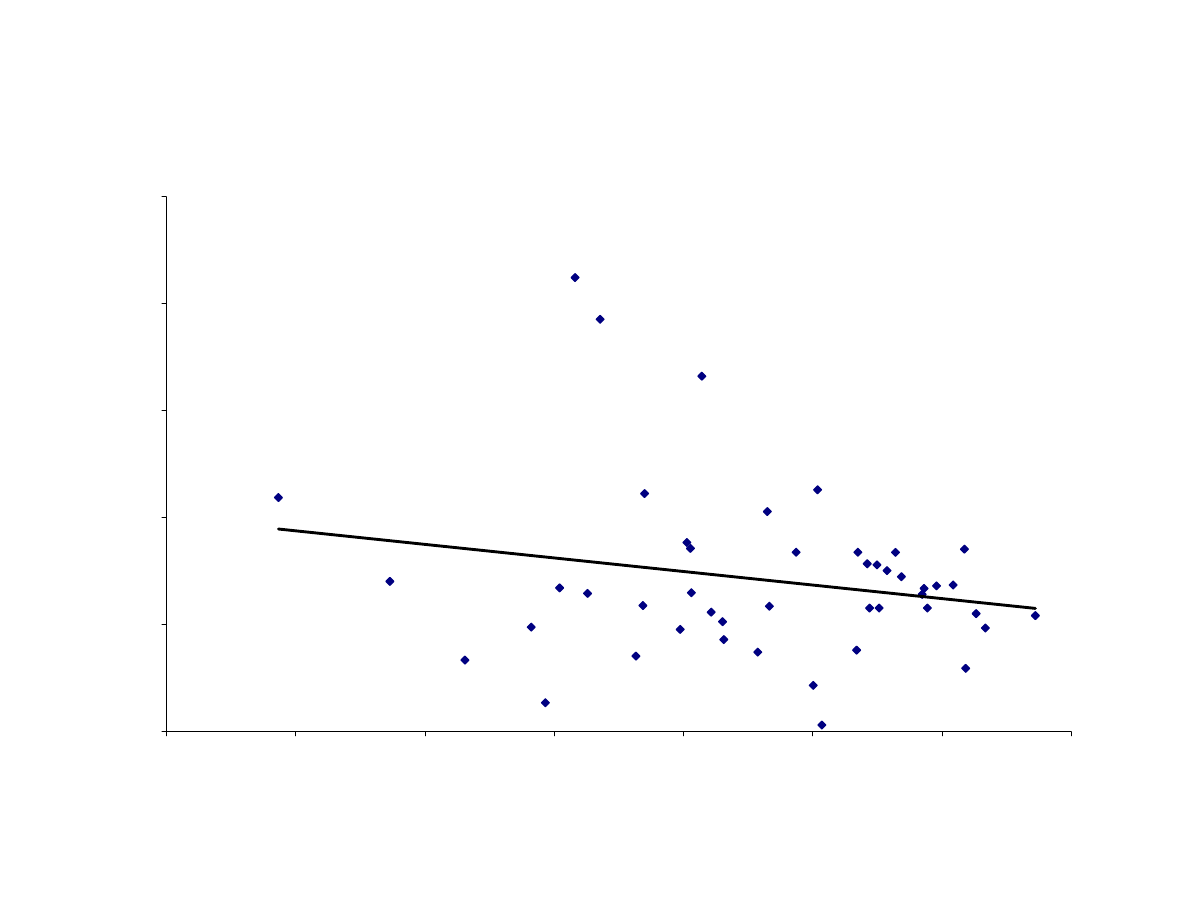
Figure 1: Regression to the Mean for Income Per Capita

y = -0.1265x + 1.7596

p-value=0.16, R

2

= 0.0429

0.00

0.50

1.00

1.50

2.00

2.50

6.00

6.50

7.00

7.50

8.00

8.50

9.00

9.50

ln(GDP65)

ln(

G

DP95/G

D

P65)

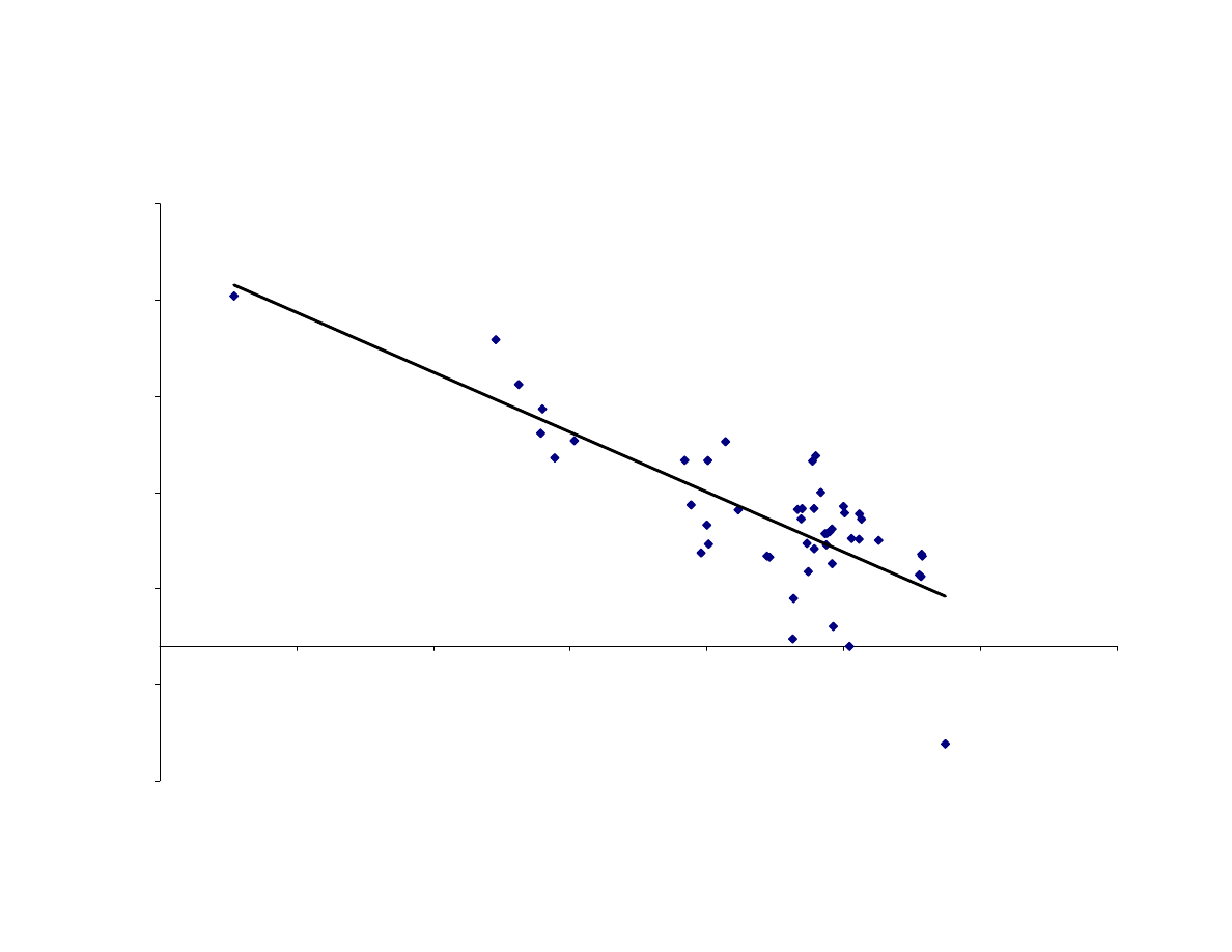
Figure 2: Regression to the Mean for Life Expectancy

y = -0.6224x + 48.477

p-value=0.00, R

2

= 0.6123

-7

-2

3

8

13

18

23

45

50

55

60

65

70

75

80

Life65

Life95-

Life65

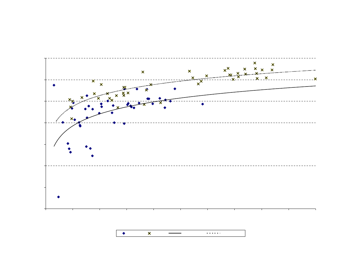
Figure 3: The Changing Relation Between Life Expectancy and Income per Capita

y = 4.051Ln(x) + 33.428

y = 3.6731Ln(x) + 40.837

45

50

55

60

65

70

75

80

0

2000

4000

6000

8000

10000

12000

14000

16000

18000

20000

GDP per capita

life ex

pec

tanc

y at bir

th

1965

1995

Log. (1965)

Log. (1995)

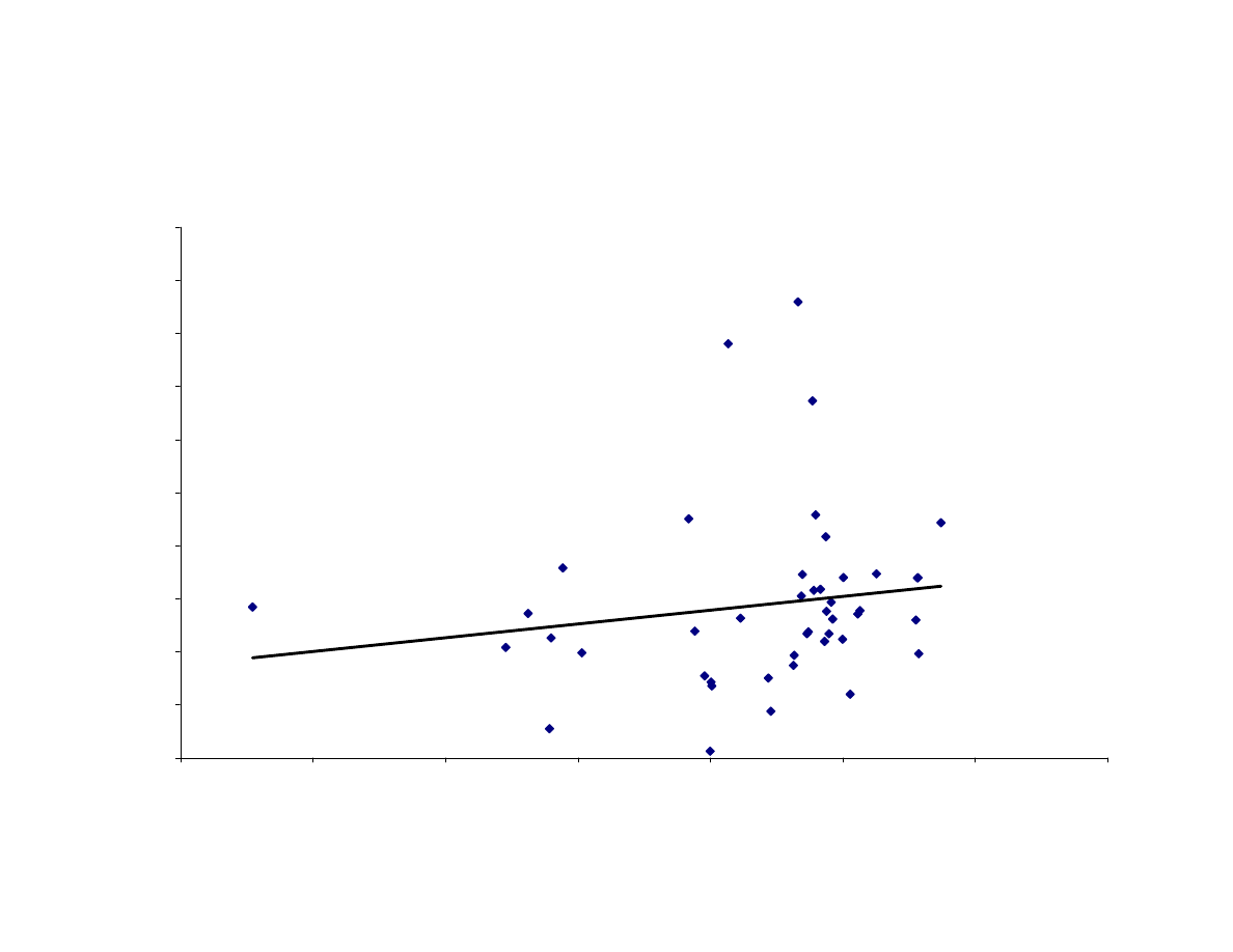
Figure 4: Regression to Mean fo the Component of Life Expectancy Changes Explained by

Changes in Income

y = 0.0519x - 0.5973

p-value = 0.29, R

2

= 0.0258

0

1

2

3

4

5

6

7

8

9

10

45.00

50.00

55.00

60.00

65.00

70.00

75.00

80.00

Life65

Change in Life Expectancy Explained

by Change in Income (1965-95)

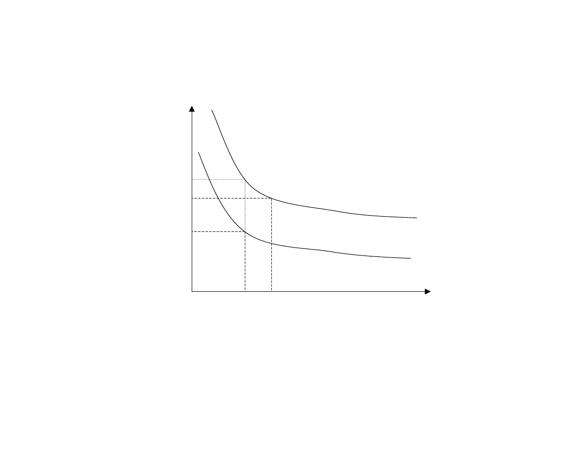
Figure 5: Income Equivalent Compensation for Life Expectancy Gains

T

Y

U

τ

U

τ+∆τ

Y

τ+∆τ

Y

τ

T

τ

T

τ+∆τ

E+ Y

τ+∆τ

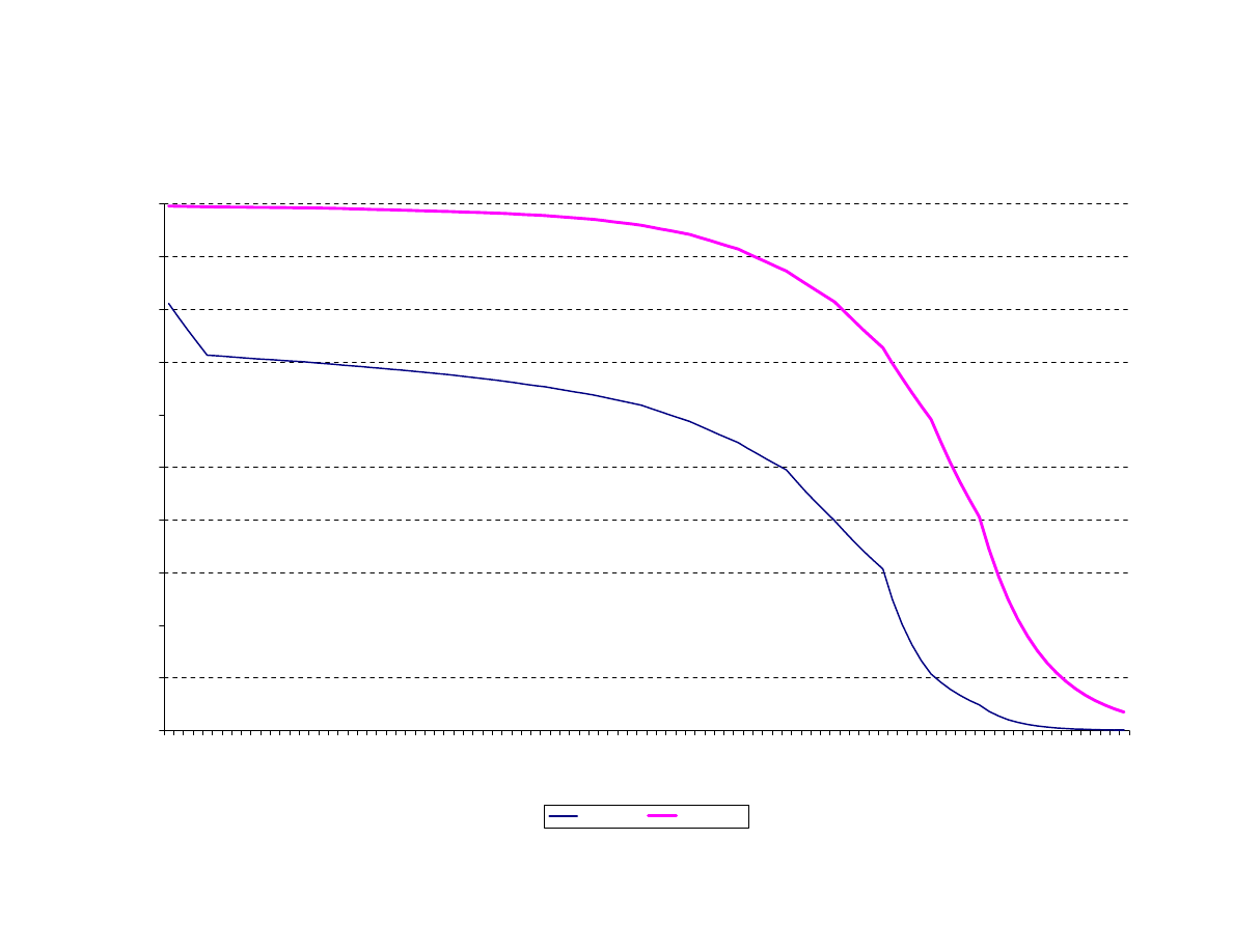
Figure 6: Survival Rate Distributions - Egypt 1965 and Japan 1995

0

0.1

0.2

0.3

0.4

0.5

0.6

0.7

0.8

0.9

1

0

3

6

9 12 15 18 21 24 27 30 33 36 39 42 45 48 51 54 57 60 63 66 69 72 75 78 81 84 87 90 93 96 99

age

S(

t,0)

-

pr

obability

of s

ur

viv

al fr

om age 0 to age t

Egypt'65

Japan'95

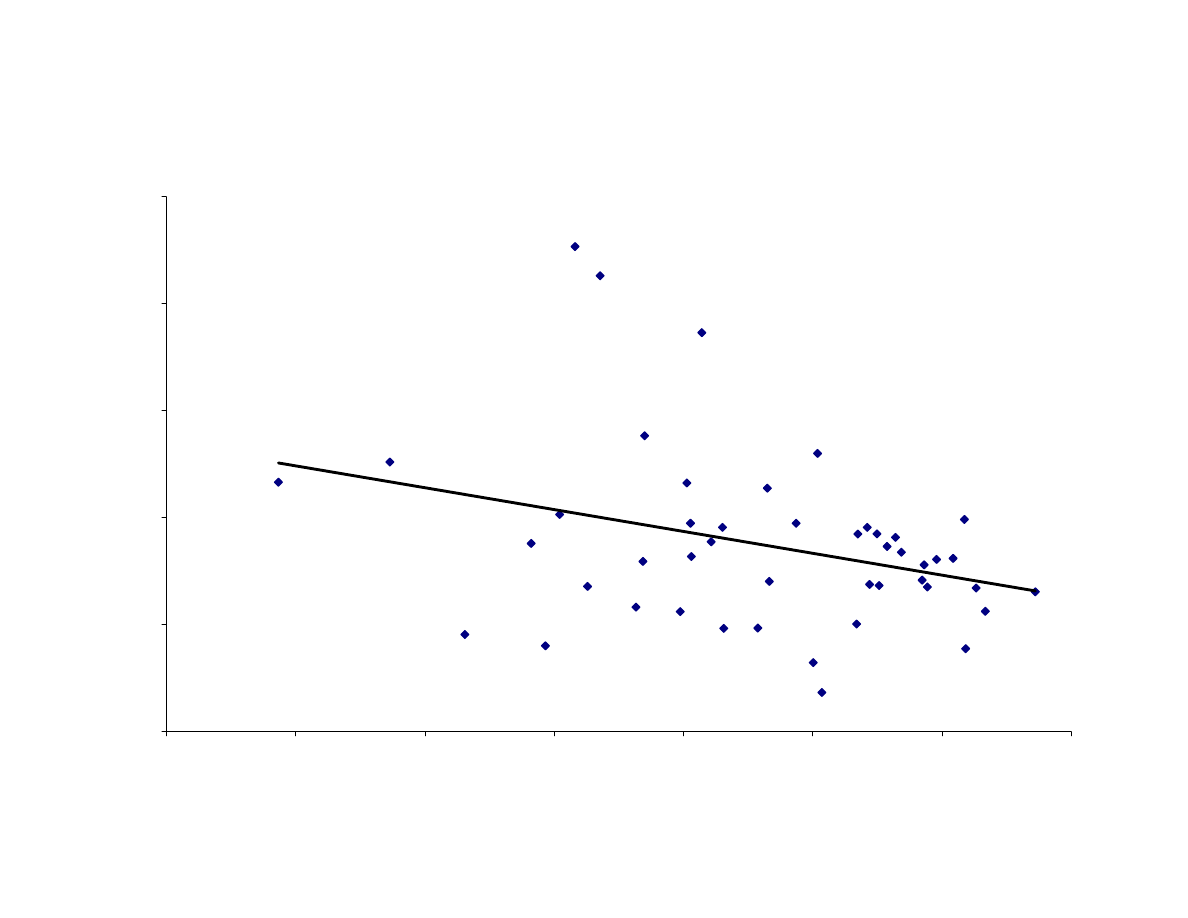
Figure 7: Regression to the Mean for Income Equivalent Compensation

y = -0.2042x + 2.5687

p-value=0.03, R

2

= 0.1031

0.00

0.50

1.00

1.50

2.00

2.50

6.00

6.50

7.00

7.50

8.00

8.50

9.00

9.50

ln(GDP65)

ln(

(G

DP95 +

Inc

Equiv

Comp)

/G

D

P65)

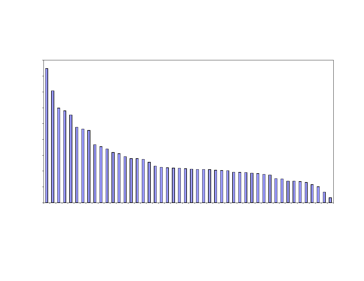
Figure 8: Share of Welfare Improvements due to Longevity Gains

0%

10%

20%

30%

40%

50%

60%

70%

80%

90%

VENEZUELA

EL SALV.

EG

YPT

CHILE

ECUADOR

MEXICO

COSTA RICA

COLOMBIA

ARG

E

NTINA

MAURITIUS

YUG

O

S

LAVIA

PORTUGAL

PHILIPPINES

TRIN. & TOB.

URUGUAY

BARBADO

S

NEW ZEAL.

ITALY

AUSTRALIA

AUSTRIA

USA

HONG KONG

PUERTO

RICO

JAPAN

CANADA

N. IRELAND

GE

RMA

N

Y

SING

APO

RE

LUXEMB.

SPAIN

SCO

T

LAND

FRANCE

BELG

IUM

ENG

L. & WALES

PO

LAND

FINLAND

G

R

EECE

SWEDEN

IRELAND

MALTA

ICELAND

BELIZE

HUNGARY

NETHERL.

NORWAY

ROMANIA

CZECHOSL.

BULG

ARIA

country